Using Prediction Markets to Track Information Flows:  Evidence from Google1 

 

Bo Cowgill Google 

   

Justin Wolfers Wharton, U. Penn NBER, CEPR, IZA 

  

Eric Zitzewitz Dartmouth College 

     January 2009 

Abstract 

In the last three years, Google has conducted the largest corporate experiment with prediction markets we are aware of.  In this paper, we illustrate how markets can be used to study how an organization processes information.  We document a number of biases in Google’s markets, most notably an optimistic bias.  Newly hired employees are on the optimistic side of these markets, and optimistic biases are significantly more pronounced on days when Google stock is appreciating.  We find correlated trading among employees who sit within a few feet of one another and employees with social or work relationships.  The results are interesting in light of recent research on the role of optimism in entrepreneurial firms, as well as recent work on the importance of geographic and social proximity in explaining information flows in firms and markets. 

 

                                                            1  Cowgill:  Bcowgill@google.com.  Wolfers:  Jwolfers@wharton.upenn.edu.  Zitzewitz (corresponding author): 6016 Rockefeller Hall, Hanover, NH 03755.  (603) 646‐2891.  Fax:  (603) 646‐2122.  Eric.zitzewitz@dartmouth.edu.  http://www.dartmouth.edu/~ericz/.  The authors would like to thank Google for sharing the data used in this paper and Susan Athey, Gary Becker, Jonathon Cummings, Stefano DellaVigna, Harrison Hong, Larry Katz, Steven Levitt, Ulrike Malmendier, Kevin M. Murphy, Michael Ostrovsky, Paul Oyer, Parag Pathak, Tanya Rosenblat, Richard Schmalensee, Jesse Shapiro, Kathryn Shaw and seminar participants at the AEA meetings, Chicago, Google, the Kaufmann Foundation, INFORMS, the NBER Summer Institute, the Stanford Institute for Theoretical Economics, and Wesleyan for helpful suggestions and comments.  Many individuals at Google contributed to Google’s prediction markets and provided useful input to our work.  We would specifically like to thank Diana Adair, Doug Banks, Laszlo Bock, Todd Carlisle, Alan Eustace, Patri Friedman, Robyn Harding, Susan Infantino, Bill Kipp, Jennifer Kurkoski, Ilya Kyrnos, Piaw Na, Amit Patel, Jeral Poskey, Chris Powell, Jonathan Rosenberg, Prasad Setty, Hal Varian, Brian Welle, the Google HR Analytics Team, and the traders in Google’s prediction market. 

  

Using Prediction Markets to Track Information Flows:  Evidence from Google 

In the last 4 years, many large firms have begun experimenting with internal prediction markets 

run among their employees.2  The primary goal of these markets is to generate predictions that 

efficiently aggregate many employees’ information and augment existing forecasting methods.  

Early evidence on corporate markets’ performance has been encouraging (Ortner, 1998; Chen 

and Plott, 2002; this paper). 

In this paper, we argue that in addition to making predictions, internal prediction can 

provide insight into how organizations process information.  Prediction markets provide 

employees with incentives for truthful revelation and can capture changes in opinion at a much 

higher frequency than surveys, allowing one to track how information moves around an 

organization and how it responds to external events. We exemplify this use of prediction 

markets with an analysis of Google’s internal markets, the largest corporate prediction market 

we are aware of. 

We can draw two main conclusions.  The first is that Google’s markets, while reasonably 

efficient, reveal some biases.  During our study period, the internal markets overpriced 

securities tied to optimistic outcomes by 10 percentage points.3  The optimistic bias in Google’s 

markets was significantly greater on and following days when Google stock appreciated.  

Securities tied to extreme outcomes were underpriced by a smaller magnitude, and favorites 

were also overpriced slightly.  These biases in prices were partly driven by the trading of newly 

hired employees; Google employees with longer tenure and more experience trading in the 

markets were better calibrated.  Perhaps as a result, the pricing biases in Google’s markets 

                                                            2  Apart from Google, firms whose internal prediction markets have been mentioned in the public domain include Abbott Labs, Arcelor Mittal, Best Buy, Chrysler, Corning, Electronic Arts, Eli Lilly, Frito Lay, General Electric, Hewlett Packard, Intel, InterContinental Hotels, Masterfoods, Microsoft, Motorola, Nokia, Pfizer, Qualcomm, Siemens, and TNT.  Of the firms for which we know the rough size of their markets, Google’s are by far the largest in terms of both the number of unique securities and participation. 3  In Google’s markets, as in many other corporate prediction markets, participants begin with an endowment of artificial currency (called “Goobles” in Google’s case).  Participants can use this currency to “purchase” “securities” that pay off in Goobles if a specified event occurs.  While we follow the academic literature and use the terms “purchase” and “security” in describing Google’s markets, it is important to note that legally Google employees are not trading securities as defined under securities laws in that they are not placing real money at risk.  

1  

declined over our sample period, suggesting that corporate prediction markets may perform 

better as collective experience increases. 

The second conclusion is that opinions on specific topics are correlated among 

employees who are proximate in some sense.  Physical proximity was the most important of 

the forms of proximity we studied.  Physical proximity needed to be extremely close for it to 

matter.  Using data on the precise latitude and longitude of employees’ offices, we found that 

prediction market positions were most correlated among employees sharing an office, that 

correlations declined with distance for employees on the same floor of a building, and that 

employees on different floors of the same building were no more correlated than employees in 

different cities.4  Google employees moved offices extremely frequently during our sample 

period (in the US, approximately once every 90 days), and we are able to use these office 

moves to show that our results are not simply the result of like‐minded individuals being seated 

together. 

Other forms of proximity mattered too. Google employees who had worked 

concurrently on the same project, reviewed each other’s code, or were within 1‐2 steps on the 

organizational chart had more correlated trading.  Most measures of demographic similarity 

(we checked 8 measures) were not associated with higher position correlations, but sharing 

native speaking ability in English or a common non‐English native language was in some 

specifications.       

  The results about demographics not affecting information sharing significantly are 

interesting given that participants in Google’s prediction markets were decidedly not 

representative of the organization as a whole.  Participants were more likely to be in 

programming roles at Google, located on either the main (Mountain View, CA) or New York 

campuses, and, within Mountain View, located closer to the center of campus.  In addition, 

participation was higher among those with more quantitative backgrounds (as evidenced by 

undergraduate major or aptitude test scores) and more interest in either investing or poker (as 

                                                            4  As discussed below, in all data analyzed by the external researchers on this project, Google employees were anonymized and identified only by an ID# that was used to link datasets. 

2  

evidenced by participation on related email lists).  The fact that trading positions were not 

correlated along most of these dimensions (physical geography being the exception) suggested 

that even if the market participants were not representative of Google, the people they were 

sharing information with might be more so.   

These results contribute to three quite different literatures: on the role of optimism in 

entrepreneurial firms, on employee communication in organizations, and on social networks 

and information flows among investors.  De Meza and Southey (1996) argue many of the 

stylized facts about entrepreneurship are consistent with an “entrepreneur’s curse” in which 

firms are started by those most overly optimistic about their prospects.  Evidence from 

experiments and the field (Cramerer and Lovallo, 1999; Arabsheibani, et. al. 2000; Simon and 

Houghton, 2003; Astebro, 2003) suggest that entrepreneurs are indeed optimistically biased.  A 

modest optimistic bias may be a desirable for both leaders and employees in entrepreneurial 

firms, however, if it generates motivation (Benabou and Tirole, 2002 and 2003; Compte and 

Postlewaite, 2004), leads to risk‐taking that generates positive externalities (Bernardo and 

Welch, 2001; Goel and Thakor, 2007), or makes employees cheaper to compensate with stock 

options (Oyer and Schaefer, 2005).  We contribute to this literature by documenting optimism 

among the employees of an important entrepreneurial firm, as well as by showing a strong link 

between optimistic bias and recent stock market performance. 

Communication between managers and workers and among peers has long been 

viewed as an important determinant of optimal organizational structure (Bolton and 

Dewatripont, 1994; Harris and Raviv, 2002; Dessein, 2002), with improvements in 

communication technology making more efficient structures possible (Chandler, 1962 and 

1990; Rajan and Wulf, 2006).  Most work on geography and communication within firms or 

teams has studied intercity collaboration, finding that geography’s importance appears to have 

declined with communication costs (e.g., Kim, Morse, and Zingales, 2007), although time zone 

differences still matter (e.g., O’Leary and Cummings, 2007). 

Despite rather significant advances in communication technology, many innovative 

firms and their employees pay significantly higher costs to cluster in places like Silicon Valley 

3  

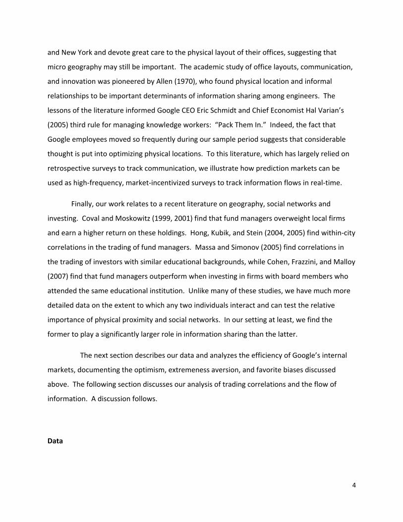
and New York and devote great care to the physical layout of their offices, suggesting that 

micro geography may still be important.  The academic study of office layouts, communication, 

and innovation was pioneered by Allen (1970), who found physical location and informal 

relationships to be important determinants of information sharing among engineers.  The 

lessons of the literature informed Google CEO Eric Schmidt and Chief Economist Hal Varian’s 

(2005) third rule for managing knowledge workers:  “Pack Them In.”  Indeed, the fact that 

Google employees moved so frequently during our sample period suggests that considerable 

thought is put into optimizing physical locations.  To this literature, which has largely relied on 

retrospective surveys to track communication, we illustrate how prediction markets can be 

used as high‐frequency, market‐incentivized surveys to track information flows in real‐time.  

Finally, our work relates to a recent literature on geography, social networks and 

investing.  Coval and Moskowitz (1999, 2001) find that fund managers overweight local firms 

and earn a higher return on these holdings.  Hong, Kubik, and Stein (2004, 2005) find within‐city 

correlations in the trading of fund managers.  Massa and Simonov (2005) find correlations in 

the trading of investors with similar educational backgrounds, while Cohen, Frazzini, and Malloy 

(2007) find that fund managers outperform when investing in firms with board members who 

attended the same educational institution.  Unlike many of these studies, we have much more 

detailed data on the extent to which any two individuals interact and can test the relative 

importance of physical proximity and social networks.  In our setting at least, we find the 

former to play a significantly larger role in information sharing than the latter.     

     The next section describes our data and analyzes the efficiency of Google’s internal 

markets, documenting the optimism, extremeness aversion, and favorite biases discussed 

above.  The following section discusses our analysis of trading correlations and the flow of 

information.  A discussion follows. 

 

Data   

4  

The data used in our analysis was collected in anonymized format from a variety of different 

internal Google sources.  We made use of Google’s data about employees’ office locations and 

a database of office moves.  For four of Google’s U.S. campuses (Mountain View, CA; New York, 

NY; Phoenix, AZ; Kirkland, WA), this data includes the precise latitude and longitude of the 

offices.  Our analysis also used the results of an internal April 2006 survey about employee 

backgrounds and social networks, and anonymized records of code reviews, project 

assignments, email list memberships, and reporting relationships.  All data we used was 

summarized and/or anonymized before analysis. 

Google’s prediction markets were launched in April 2005.  The markets are patterned on 

the Iowa Electronic Markets (Berg, et. al., 2001).  In Google’s terminology, a market asks a 

question (e.g., “how many users will Gmail have?”) that has 2‐5 possible mutually exclusive and 

completely exhaustive answers (e.g., “Fewer than X users”, “Between X and Y”, and “More than 

Y”).  Each answer corresponds to a security that is worth a unit of currency (called a “Gooble”) if 

the answer turns out to be correct (and zero otherwise). Trade is conducted via a continuous 

double auction in each security. As on the IEM, short selling is not allowed; traders can instead 

exchange a Gooble for a complete set of securities and then sell the ones they choose.  

Likewise, they can exchange complete set of securities for currency. There is no automated 

market maker, but several employees did create robotic traders that sometimes played this 

role. 

Each calendar quarter from 2005Q2 to 2007Q3 about 25‐30 different markets were 

created.  Participants received a fresh endowment of Goobles which they could invest in 

securities. The markets’ questions were designed so that they could all be resolved by the end 

of the quarter. At the end of the quarter, Goobles were converted into raffle tickets and prizes 

were raffled off.  The prize budget was $10,000 per quarter, or about $25‐100 per active trader 

(depending on the number active in a particular quarter). Participation was open to active 

5  

employees and some contractors and vendors; out of 6,425 employees who had a prediction 

market account, 1,463 placed at least one trade.5 

 Table 1 provides an overview of the types of questions asked in Google’s markets.  

Common types of markets included those forecasting demand (e.g., the number of users for a 

product) and internal performance (e.g., a product’s quality rating, whether a product would 

leave beta on time).  Much smaller scale experiments in these uses of prediction markets have 

been documented at other companies (e.g., by Chen and Plott, 2002 and Ortner, 1998, 

respectively).  Markets were also run on company news that did not directly imply performance 

(e.g., will a Russia office open?) and on features of Google’s external environment that might 

affect its planning (e.g., the mix of hardware and software used to access Google). 

In addition, about 30 percent of Google’s markets were so‐called “fun” markets – 

markets on subjects of interest to its employees but with no clear connection to its business 

(e.g., the quality of Star Wars Episode III, gas prices, the federal funds rate).  Other firms 

experimenting with prediction markets that we are aware of have avoided these markets, 

perhaps out of fear of appearing unserious.  Interestingly, we find that volume in “fun” and 

“serious” markets are positively correlated (at the daily, weekly, and monthly frequencies), 

suggesting that the former might help create, rather than crowd out, liquidity for the latter. 

Table 2 provides summary statistics on the participants in Google’s prediction markets.  

As noted above, participants are not representative of Google employees as a whole: on many 

dimensions, they are closer to the modal employee than the mean.  They are more likely to be 

programmers, as measured by being in the Engineering department, having participated in a 

code review, or having majored in Computer Science.  Across several measures, they are more 

quantitatively and stock‐market‐oriented (more likely to be in a quantitative role, have a 

quantitative degree, or participate on investing, economics, or poker‐related email lists).  They 

are more likely to be based in Google’s Mountain View and New York campuses. Within 

                                                            5  By way of comparison, Google is listed in COMPUSTAT has having 5,680 and 10,674 employees at the end of calendar years 2005 and 2006, respectively.  We excluded from our analyses a small number of trades that were placed after an event happened (but before the market was closed and expired) or were self‐trades (which resulted from the fact that the software allowed traders to be matched with their own limit orders). 

6  

Mountain View, they are more likely to have offices close to the center of campus.  They have 

been employed longer, are less likely to leave after our sample ends, and are more deeply 

embedded in the organization across a number of measures (they subscribe to more email lists, 

name more professional contacts, and are more likely to have been named by someone at 

Google as a friend).  They are also slightly more senior (as measured by levels from the CEO) 

than non‐participants.  Regressions predicting participation in Table 3 largely confirm these 

results in a multivariate context. 

 

The Efficiency of Google’s Markets 

Google’s prediction markets are reasonably efficient, but did exhibit four specific biases:  an 

overpricing of favorites, short aversion, optimism, and an underpricing of extreme outcomes.  

New employees and inexperienced traders appear to suffer more from these biases, and as 

market participants gained experience over the course of our sample period, the biases become 

less pronounced. 

A simple test of a prediction market’s efficiency is to ask whether, when a security is 

priced at X, it pays X in expectation.  In Figure 1, we sort trades in the Google markets into 20 

bins based on their price (0‐5, 5‐10, etc.) and plot the average price and ultimate payoff.  The 

standard errors for the average payoff of a bin are adjusted for clustering of outcomes within a 

market.6  The results suggest a slight (and marginally statistically significant) overpricing of 

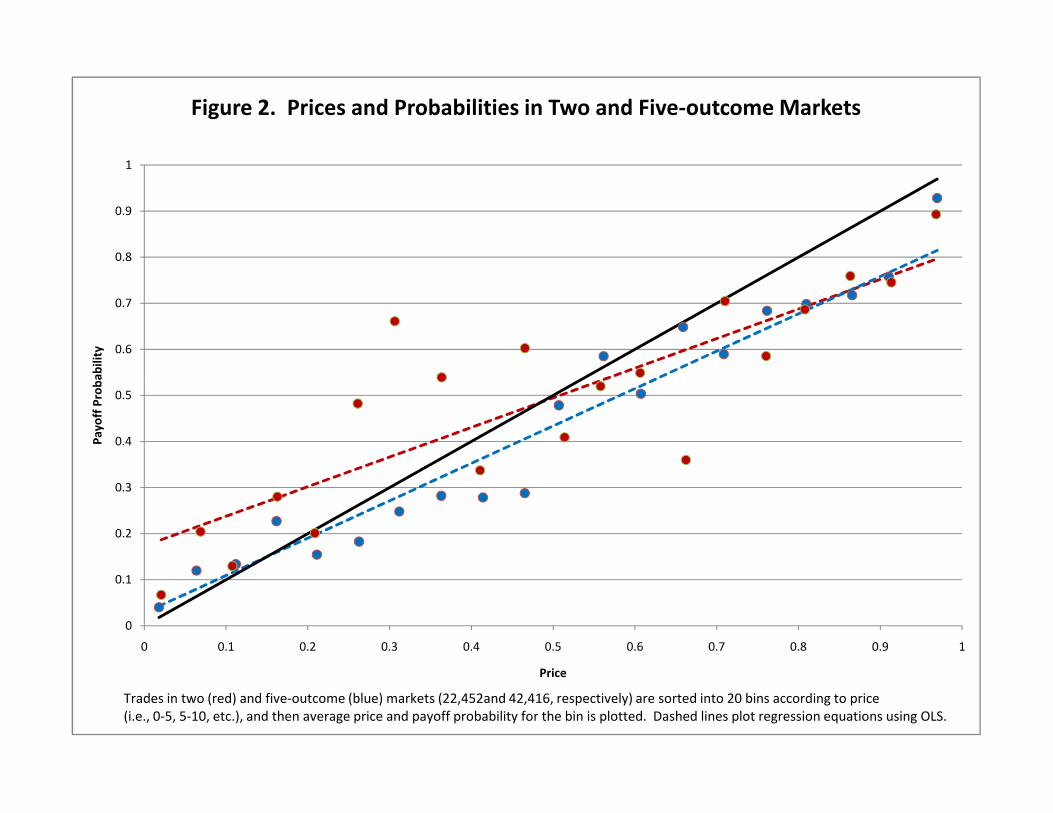
favorites and underpricing of longshots.  Figure 2 conducts the analysis separately for 2 and 5‐

outcome markets (which account for 29 and 57 percent of the markets, respectively).  The two 

outcome markets exhibit positive returns for securities priced below 0.5, while the five 

outcome markets exhibit positive returns for securities priced below 0.2, confirming that a 

reverse favorite‐longshot bias is a useful way of characterizing this predictability. 

                                                            6  Clustering standard errors by market allows for any relationship in the error terms of observations from the same market.  In our case, returns to expiry for different trades of the same security will be positively correlated, while returns to expiry for different securities will be negatively correlated.  Monte Carlo simulations in Zitzewitz (2008) find that clustering standard errors of groups of related derivatives produces uniformly distributed p‐values under the null hypothesis.  

7  

Table 4 presents regressions of returns to expiry on the difference between the 

transaction price and 1/N (where N is the number of outcomes).  We use this functional form 

for two reasons:  1) the difference between price and 1/N captures the extent to which a 

contract is a favorite and 2) the non‐parametric analysis in Figure 2 suggests that this form 

would describe the data well.  These regressions provide statistically significant evidence of a 

reverse favorite‐longshot bias (or favorite bias, for short).  The bias is present to a roughly equal 

extent in subsamples of the data (2 and 5 outcome markets; fun and serious markets).  Since 

these results could be driven by microstructure‐driven noise in prices (e.g., due to bid‐ask 

bounce), we repeat these tests using lagged prices, bid‐ask midpoints, and after limiting the 

same to trades conducted inside the arbitrage‐free bid‐ask spread.7  The favorite bias is robust 

to these alternative specifications. 

The presence of a favorite bias is somewhat surprising in light of Ali (1977) and Manski’s 

(2006) theoretical analysis, as well as the evidence of a longshot bias in public prediction 

markets (Tetlock, 2004; Zitzewitz, 2006; Leigh, Wolfers, and Zitzewitz, 2008).  Ali and Manski 

point out that because traders can take larger positions for a given amount of downside risk 

when betting on longshots, when traders are liquidity constrained (and risk‐neutral), we should 

expect the prices of longshots (favorites) to be above (below) the median probability belief.  If 

median probability beliefs are unbiased, this should result in a longshot bias in prices.  Given 

that these assumptions of liquidity‐constraints and risk‐neutrality seem more likely to hold for a 

corporate prediction market than for a public prediction market, especially one like Intrade.com 

where account sizes are not constrained, this makes the finding of a favorite bias in Google’s 

markets particularly surprising.  One possibility is that the favorite bias in prices reflects a larger 

favorite bias in the beliefs of the median trader.      

                                                            7  In an IEM‐style prediction market, one can increase one’s exposure a given security by either purchasing the security or by exchanging $1 for a bundle of securities track all possible outcomes in a given market and then selling the other components of the bundle.  We calculate the “arbitrage‐free” ask as the cheapest way of acquiring the security, i.e. the minimum of the ask for the security and one minus the sum of the bids for the other securities. We do the analogous calculation to determine the arbitrage‐free bid.  The arbitrage‐free mid point is the average of the arbitrage‐free bid and ask.  For 70 of 70,706 trades, the pre‐trade arbitrage‐free ask was actually below the arbitrage‐free bid, implying that there was an arbitrage opportunity to either buy or sell all securities in a bundle.  In these cases, we also used the midpoint as an indicator of the securities value. 

8  

Table 5 calculates returns from purchasing securities, which are negative and 

statistically significant on average.  This suggests some traders may be adverse to short selling 

securities.  As further evidence of short aversion, in order book snapshots collected each time 

an order was placed, we found 1,747 instances where the bid prices of the securities in a 

particular market added to more than 1, implying an arbitrage opportunity (from buying a 

bundle of securities for $1 and then selling the components). In constant, we found only 495 

instances where the ask prices added to less than 1 (implying an arbitrage opportunity of 

buying the components of a bundle for less than $1 and then exchanging the bundle). 

Table 5 also calculates returns according to whether the security’s outcome would be 

good news for Google.  For some markets, such as markets on “fun” or “external news” topics, 

it was not clear which outcome was better for Google, so we are able to rank outcomes for 157 

out of 270 markets.  Of these 157, all but 11 have either 2 or 5 outcomes, and so, for simplicity, 

the table restricts attention to these.  In two‐outcome markets, the optimistic (i.e. better for 

Google) outcome is significantly overpriced:  it trades at an average price of 46 percent but 

these trades earn average returns to expiry of ‐26 percentage points.  The pessimistic outcome 

is underpriced by a similar margin.  Five‐outcome markets display a small amount of optimism 

bias but primarily an overpricing of intermediate outcomes; the third‐best outcome out of five 

is priced at 30 but earns returns to expiry of ‐12 percentage points.8  We refer to this bias as 

extreme aversion. 

Table 6 measures the extent of the optimism bias in subsamples of the data.  The 

optimistic bias exists entirely in the two categories of contracts where outcomes are most 

directly under the control of Google employees:  company news (e.g., office openings) and 

performance (e.g., project completion and product quality).  Markets on demand and external 

news with implications for Google are not optimistically biased.  Optimistic bias is larger in two 

outcome markets, early in our sample period, and earlier in each quarter. 

                                                            8  All the averages in Figure 1 and Tables 4‐6 are trade rather than contract‐weighted.  If a contract’s future price path is correlated with whether it trades in the future, contract‐weighted analysis of efficiency can suffer from a look‐ahead bias.    

9  

Table 7 provides tests for whether these biases are independent of one another, finding 

that they largely are.  The final column in Table 7 interacts the four biases (optimism, favorite 

bias, extreme aversion, and short aversion) with a date variable (scaled to equal 0 at the 

beginning of our sample on April 7, 2005 and 1 at the end on September 30, 2007).  The 

coefficients on these interactions suggest that Google’s markets became significantly less 

biased over the course of our sample period.  In the final column of Table 7, we find that 

weighting trades by the number of shares transacted, rather than equally, reduces the 

estimated magnitude of the biases. 

Three of the four biases (optimism, extreme aversion, and favorite bias) could reflect ex 

post surprise rather than ex ante biases in beliefs:  Google’s outcomes during this time period 

could simply have been more disappointing, more extreme, and harder to predict than rational 

traders anticipated.  Google’s stock price more than tripled during our time period (April 2005 

to September 2007), casting doubt on a negative ex post surprise as the explanation.  

Furthermore, most of the appreciation occurred during 2005, the period in which the apparent 

optimistic bias in Google’s markets was greatest.   

Further evidence that there is a behavioral component to the optimism comes from 

Table 8, which examines how the optimistic bias in Google’s markets varies with very recent 

Google stock returns.  Cowgill and Zitzewitz (2008) report that employee job satisfaction is 

higher on days that Google stock appreciates, that this effect lasts one or two days, and that 

appreciation is accompanied by lower work effort and tougher grading of job candidates and 

ideas.  In this paper, we find that the overpricing of optimistic securities in Google’s prediction 

markets becomes more pronounced on days Google stock appreciates. 

The coefficient of ‐10.5 in column 1 can be interpreted as showing that, on average, 

optimistic securities earn returns to expiry that are 10.5 percentage points lower than neutral 

securities.  The coefficient of 2.2 on the interaction of optimism and prior day returns implies 

that this pricing bias is 4.4 percentage points larger following a day with 2.0 percent higher 

Google stock returns (one standard deviation during this time period).  Further tests reveal that 

this pricing bias appears to mean revert after one day and is robust to controlling for day of the 

10  

week effects and the returns on the S&P 500 and Nasdaq composite.9  Evidence of an impact of 

stock price movements on the optimism bias persists when we volume‐weight, rather than 

equal‐weight, trades. 

Who is driving these biases?  If we predict whether a trader will trade with or against 

these biases using the individual characteristics in Table 9, we find several relationships.  Newly 

hired employees are significantly more likely to take optimistic positions than other employees.  

In further tests omitted for space reasons, we find that this is especially true for contracts in the 

“Performance” and “Company News” categories in which prices are optimistically biased on 

average.  On the other hand, newly hired employees are more likely to sell favorites and to 

build positions by selling rather than purchasing securities, i.e. to trade in a way that takes 

advantage of the reverse favorite‐longshot and short aversion bias in prices.  Coders are like 

newer employees in that they trade optimistically (which lowers their returns), but also trade in 

a way that takes advantage of favorite and short aversion biases.  More experienced traders 

trade in a way that profits from optimism, favorite, and short aversion biases, but contributes 

to extreme aversion. 10 

In summary, while Google’s prediction markets grew more efficient over time, they did 

exhibit pricing predictabilities during our sample period.  These pricing predictabilities likely 

arise from short aversion, as well as from optimistic, extremeness aversion, and favorite biases 

in the market‐weighted average beliefs of Google’s employees.  To better understand how 

Google processes information as an organization, we turn to the question of whether we can 

use its prediction markets to understand how information moves around the organization. 

 

Measuring the Flow of Information                                                             9 The underpricing of extreme outcomes and longshots, in contrast, is not statistically significantly related to the sign or magnitude of prior stock day returns. 10  One trader in Google’s markets wrote a trading robot that was extremely prolific and ended up participating in about half of all trades.  Many of these trades exploited arbitrage opportunities available from simultaneously selling all securities in a bundle.  In order to avoid having this trader dominate the (trade‐weighted) results in Table 9, we include a dummy variable to control for him or her.  None of the results discussed in the above paragraph are sensitive to removing this dummy variable.   

11  

In this section we aim to understand how information and opinions are shared by testing 

whether employees who are proximate to each other trade in a correlated manner.  We 

develop measures of geographical, organizational, and social proximity, and also measure 

demographic similarity. 

Our analysis aims to understand which of these measures of proximity is related to 

correlations in information and opinion, as expressed in prediction market trading.  We follow 

an approach similar to the prior studies cited above that test for communication in securities 

markets, in that we test for correlations between the trading and prior positions of those who 

are proximate along some dimension.  We design our approach to take into account of the fact 

that we are testing the relative importance of alternative forms of proximity, that we have 

trade‐by‐trade rather than quarterly holdings data, and that our markets are comparatively 

short‐lived. 

In order to take maximum advantage of our data, we conduct our analysis at the trade 

level.  In most of our tests, we take the participants in each trade to be exogenous, and use the 

prior positions of proximate colleagues to predict the size and direction of the trade.  Our 

rationale for this approach is both simplicity and the fact that exact timing of individuals’ trades 

in a low‐stakes prediction market is likely to be exogenous, since it would be largely determined 

by when they have time available (e.g., for a programmer, while code is being compiled and 

tested), but the direction and size of their trades is of course not likely to be. 

Given the likely absence of hedging motives in these markets, if trader i buys a security 

from trader j at some price, we can infer that i’s subjective belief about its payoff probability is 

higher than j’s.  Equally, if a third trader k holds a large long position in the security prior to the 

trade, we can infer that her subjective belief about the value of the security is higher than if she 

were holding a short position.  Our approach will be to test whether the buyer in a particular 

transaction is more proximate to other traders with prior long positions. 

12  

Specifically, we will estimate i’s desired holdings of security s at prevailing market prices,  

∑ , where   is the weight that i gives the opinion of k,   is 

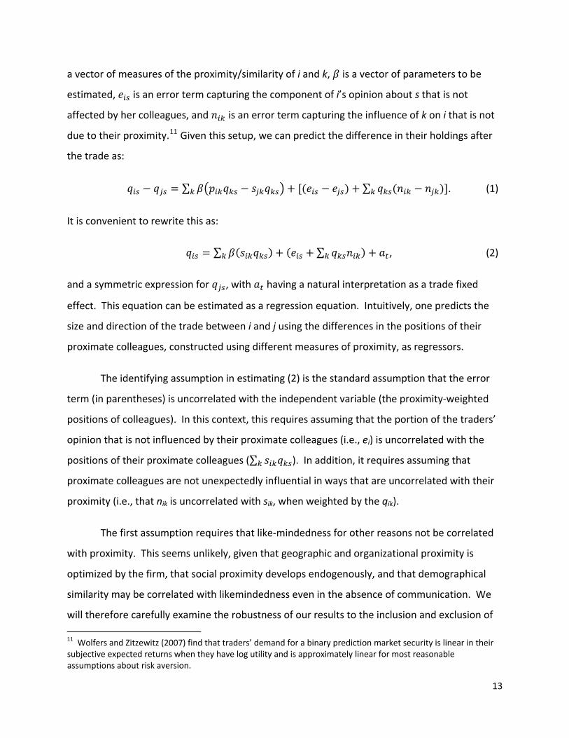
a vector of measures of the proximity/similarity of i and k,   is a vector of parameters to be 

estimated,   is an error term capturing the component of i’s opinion about s that is not 

affected by her colleagues, and   is an error term capturing the influence of k on i that is not 

due to their proximity.11 Given this setup, we can predict the difference in their holdings after 

the trade as: 

  ∑ ∑ .  (1) 

It is convenient to rewrite this as: 

  ∑ ∑ ,  (2) 

and a symmetric expression for  , with   having a natural interpretation as a trade fixed 

effect.  This equation can be estimated as a regression equation.  Intuitively, one predicts the 

size and direction of the trade between i and j using the differences in the positions of their 

proximate colleagues, constructed using different measures of proximity, as regressors. 

The identifying assumption in estimating (2) is the standard assumption that the error 

term (in parentheses) is uncorrelated with the independent variable (the proximity‐weighted 

positions of colleagues).  In this context, this requires assuming that the portion of the traders’ 

opinion that is not influenced by their proximate colleagues (i.e., ei) is uncorrelated with the 

positions of their proximate colleagues (∑ ).  In addition, it requires assuming that 

proximate colleagues are not unexpectedly influential in ways that are uncorrelated with their 

proximity (i.e., that nik is uncorrelated with sik, when weighted by the qik). 

The first assumption requires that like‐mindedness for other reasons not be correlated 

with proximity.  This seems unlikely, given that geographic and organizational proximity is 

optimized by the firm, that social proximity develops endogenously, and that demographical 

similarity may be correlated with likemindedness even in the absence of communication.  We 

will therefore carefully examine the robustness of our results to the inclusion and exclusion of                                                             11  Wolfers and Zitzewitz (2007) find that traders’ demand for a binary prediction market security is linear in their subjective expected returns when they have log utility and is approximately linear for most reasonable assumptions about risk aversion. 

13  

controls for observable forms of proximity.  Furthermore, for geographic proximity, we can 

exploit the frequency of office moves at Google to separate the effects of geographic proximity 

and like‐mindedness that may be correlated with it.   

The second assumption requires assuming that our observed measures of proximity are 

not correlated with unobserved proximity. For example, if colleagues who shared an office 

were also friends, but failed to report in on their social network survey, we would include the 

effect of their being friends as part of the effect of sharing an office.  The potential for such 

confounding effects must be kept in mind when interpreting our results. 

 We construct our dataset for estimating (2) as follows.  For each pair of our 1,463 

prediction market traders, we calculate measures of their geographic, organizational, and social 

proximity and their demographic similarity.  While our demographic similarity measures are 

constant throughout our time period and, due to data limitations, our social proximity 

measures are as well, we update our geographic and organizational proximity measures each 

week.12  As of each Sunday morning in our sample, we construct: 1) a company‐wide seating 

chart using our database of office moves, 2) an organizational chart using our history of changes 

in reporting relationships, and 3) measures of whether any two employees had concurrently 

worked on a project together or reviewed one another’s code as of the week in question.  We 

then construct measures of the geographic and organizational proximity of every pair of traders 

for that week. 

Prior to each trade, we calculate the normalized net position of each trader for each 

security.13  We then construct the proximity‐weighted sum of colleagues’ positions for each of 

the two traders along each dimension of proximity.  We then predict the size and direction of 

                                                            12  It is possible that our finding of a greater role for geographic and organizational proximity is due to the fact that we have better data for these than for social connections.  In earlier versions of our analysis, however, we also only had seating and organizational charts for a single point in time, and yet found a greater role for geographical and organizational proximity and a more limited role for social connections and demographics.   13  We calculate net positions in a security as the difference between a trader’s cumulative net purchases of a security and the average of her cumulative net purchases of all securities in that market.  For example, if there are two outcomes in a market, and trader X has made net purchases of 20 shares of outcome A and 10 shares of outcome B, we would calculate her positions as being +5 shares of A and ‐5 shares of B.  We then normalize positions across traders within each security using the standard deviation of positions at the time of the trade. 

14  

the trade using the proximity‐weighted colleague positions across the different dimensions and 

the trader’s prior position as regressors and including a trade fixed effect.  Standard errors 

allow for clustering of errors within a given trader’s trades across all securities.   

Table 10 presents estimates of (2).  The first column provides weak evidence that the 

trader from the city with a larger prior net position in a particular security is more likely to be 

the buyer in a given transaction.  The regression controls for the prior positions of the traders 

themselves, which is important to do because the direction of a trader’s trades in a given 

security is usually positive serially correlated, and we do not want to mistake this for a 

proximity effect.  Omitting this control makes our proximity results slightly stronger, while 

adding controls for lagged own positions does not meaningfully affect them. 

Subsequent columns add measures with narrower definitions of proximity.  In column 2, 

we add a term that weights colleagues according to the proximity of their buildings within a 

given campus.14  The positive coefficient on this term and the change in the same‐city 

coefficient to zero suggests that the relationship with same‐city colleagues is driven by those 

who are close together on campus.  In subsequent columns, we add terms that capture only the 

positions of even more proximate colleagues.  In each case, we find that only the most 

proximate colleagues appear to be correlated.  The final specification in column 6 implies that 

that colleagues who share an office or whose offices are located within a few feet on the same 

floor are correlated.15  Note that the coefficients can be directly compared; they tell us how to 

construct an estimate of k’s influence on I (wik) from a vector of measures of their proximity 

(sik).    

                                                            14  We construct building proximity weights as follows.  First, we calculate the geographic center of a building using the average GPS coordinates of its offices.  Next, we weight a trader’s same‐city colleagues’ positions using a weight equal to 100 feet divided by the distance between the geographic centers of their buildings; this weight is set to one for traders in the same building or buildings closer than 100 feet apart (less than 0.03% of trader pairs are this close), and it is set to zero for traders in different cities.  We obtained qualitatively similar results with alternative approaches, including numerators of up to 500 feet or using the square or square root of distance in the denominator.  The “proximity on floor” term takes the same approach, weighting colleagues on the same floor as 10 feet divided by the distance between their desks, with a maximum of one.  15 In the Mountain View and New York campuses where 69 and 9 percent of traders sit, respectively (and 76 and 11 percent of trades are placed, respectively), shared “offices” are typically groups of desks bounded by five‐foot high walls on a large, open‐plan floor. 

15  

Geographic information is missing for some traders.  For about 8 percent of trades, we 

are missing building information for the week in question, while room information is missing for 

19 percent of trades.  Many of these cases involved instances where an employee does not 

have an assigned location.  Since these employees may be less likely to develop geographically‐

driven relationships that lead to information sharing, we treat them differently, creating a 

second term with a weight equal to one the parties are in the same city, but building 

information is missing for either, and a term with a weight equal one if they are in the same 

building, but room information is missing for either.  For traders with missing information, 

these terms will be the sum of positions of colleagues in the same city or building, duplicating 

other variables in the regression.  For traders with position information, however, these terms 

will be equal to the position of colleagues in the same city or building without building or room 

information, respectively.  While including these terms does not significantly affect the 

coefficients on the other terms, we include them so the model can distinguish between 

colleagues with and without fixed positions.  The negative coefficient on the “room missing” 

term implies that colleagues with no fixed location in a building are less correlated than the 

average occupant with their same‐building colleagues. 

 Table 11 conducts a similar analysis using measures of social connections, work history, 

and organizational proximity.  We find that measures of social connections, either self‐reported 

on the April 2006 survey or inferred from subscriptions to email lists, do not explain trading 

correlations well.  A history of reviewing each other’s code or overlapping on a project does, 

however.  Adding terms that capture the portion of the organization one is in reduces the 

explanatory power of work history, and the single best explanator is being within one or two 

steps on the organization chart (i.e., sharing a manager, being someone’s manager, or being 

someone’s manager’s manager).  Adding the geographical proximity variables from Table 10 

reduces the estimated effect of organizational proximity; this reflects the fact that teams are 

usually co‐located. 

16  

Finally, adding controls for demographic similarity does not meaningfully affect the 

results.16  None of the demographic similarity terms are consistently statistically significant, 

with the partial exception of both being native English speakers or sharing a common non‐

English native language in some specifications.17  Apart from these variables, trading was if 

anything more correlated among dissimilar employees.   

The fact that the coefficient on the self‐reported friendship term turns negative when 

the work history and organizational proximity variables are added to the model suggests that 

friendship and a shared work history are correlated, and that the employees most likely to have 

correlated trading are those who are proximate organizationally or geographically and are not 

friends.  One admittedly speculative interpretation of this result is that friends have better 

things to discuss than the subjects of prediction markets, while the prediction markets provide 

a topic of conversation for those who are not friends.   

Table 12 examines the robustness of the geographic proximity results to adding the 

demographic, social, work history, and organization proximity variables to the model.  Adding 

demographic similarity variables slightly increases the estimate effect of sharing an office, while 

controlling for being 1‐2 steps away on the organizational chart reduces the same office 

coefficient slightly.  The latter change is again consistent with managers’ direct reports being 

co‐located.   

In Table 13, we exploit the frequency of office moves and, to a lesser extent, 

reorganizations, to attempt to separate causal effects of proximity from other sources of 

correlation between proximity and like‐mindedness.  Columns 1 and 4 repeat earlier 

                                                            16  We construct eight measures of demographic similarity:  sharing an undergraduate alma mater or major, both being native English speakers, sharing a common non‐English native language, either both or neither being coders (defined as employees who participated in at least one code review during our sample period), and similarity along three commonly studied demographic variables.  For the demographic characteristics that we obtained from a voluntary survey (undergraduate school and major and languages spoken), we are missing data for 65 percent of our traders (who account for 37 percent of the trades).  For pairs of traders where one has unknown demographics, we code the “same group” variables as zero.    17  In the April 2006 survey, Google employees were asked to list languages they spoke and to rate their ability from one to five, with 5 being native and 4 being fluent.  All but 2 percent of Google employees reported being at least fluent in English. Given the fact that the difference between fluency and native ability seemed likely to affect informal communication, we focused on this distinction in constructing the variable. 

17  

specifications, without and with demographic variables, respectively.  Columns 2 and 5 add 13‐

week lags of the geographic and 1‐2 steps away variables given, and columns 3 and 6 add 13‐

week leads of these variables.  None of the lead variables are statistically significant.  Assuming 

that like‐mindedness for non‐proximity reasons is persistent, this suggests that proximity is 

indeed causing correlated trading.  At the same time, the lagged effects of sharing an office or 

being 1‐2 steps away are roughly as strong as the current effects, suggesting it may take a few 

months for proximity to produce relationships that lead to information sharing. 

Table 14 estimates the model for different types of contracts.  We find that proximity is 

less associated with correlated trading for markets on performance and company news 

subjects, which are also the markets that exhibit a strong optimism bias.  One possible 

explanation for this difference is that these subjects are more politically sensitive, and 

therefore traders are more likely to keep their true beliefs to themselves.  We tested for 

separately for proximity effects from colleagues who were taking optimistic (i.e. betting 

outcomes that were good for Google) and pessimistic positions and found no significant 

differences. 

Table 15 considers the robustness of our results to variations in methodology.  Column 1 

repeats as a baseline the specification from Table 12, column 6, Table 13, column 4, and Table 

14, column 1.  The next column drops controls for the traders’ initial positions from the model, 

which as mentioned above tends to strengthen results.  Column 3 uses the sums of the signs of 

colleagues’ positions rather than normalized colleague positions in constructing the proximity 

terms.  Column 4 predicts (using a linear model) the direction of trade rather than its direction 

and normalized size.  Column 5 calculates colleague’s positions from 24 hours before the trade 

in question.  In general these modifications to the methodology do not affect conclusions about 

geographical and organizational proximity, with the exception of using 24‐hour‐lagged 

colleague’s positions.  The weaker results in this specification suggest that much of the sharing 

of information with proximate colleagues may occur shortly after trades are placed.  This story 

would again be consistent with prediction market topics being a topic of causal interest, as 

opposed to employees’ main job function.  

18  

With the exception of the last model, the conclusion that geographic and organizational 

proximity is associated with correlated trading is robust to alternative approaches.  The fact 

that significance is lost in the last column suggests that communication about prediction market 

topics and trading happens at high frequency.  Since account sizes in Google’s markets are 

limited, one plausible story is that traders take the maximum possible position for themselves 

and then tell their office or teammates about a security that in their view remains mispriced.  

     

Discussion 

In the past few years, many companies have experimented with prediction markets.  In this 

paper, we analyze the largest such experiment we are aware of.  We find that prices in Google’s 

markets closely approximated event probabilities, but did contain some biases, especially early 

in our sample.   The most interesting of these was an optimism bias, which was more 

pronounced for subjects under the control of Google employees, such as whether a project 

would be completed on time or whether a particular office would be opened.  Optimism was 

more present in the trading of newly hired employees, and was significantly more pronounced 

on and immediately following days with Google stock price appreciation.  Our optimism results 

are interesting given the role that optimism is often thought to play in motivation and the 

success of entrepreneurial firms.  They raise the possibility of a “stock price‐optimism‐

performance‐stock price” feedback that may be worthy of further investigation. 

We also examine how information and beliefs about prediction market topics move 

around an organization.  We find a significant role for micro‐geography.  The trading of 

physically proximate employees is correlated, and only becomes correlated after the employees 

begin to sit near each other, suggesting a causal relationship.  Work history and organizational 

proximity play a detectable, but significantly smaller, role, while social connections and 

demographics have little explanatory power. 

An important caveat to our results is that they tell us about information flows about 

prediction market subjects, many of which are ancillary to employees’ main jobs.  This may 

19  

explain why physical proximity matters more than work relationships – if prediction market 

topics are lower‐priority subjects on which to exchange information, then information 

exchange may require the opportunities for low‐opportunity‐cost communication created by 

physical proximity.  Of course, introspection suggests that genuinely creative ideas often arise 

from such low‐opportunity‐cost communication.  Google’s frequent office moves and emphasis 

on product innovation may provide an ideal testing ground in which to better understand the 

creative process. 

 

   

20  

References  Ali, Mukhtar.  1977.  “Probability and Utility Estimators for Racetrack Bettors”, Journal of 

Political Economy, 85(4), 803‐815.  Allen, Thomas.  1970.  “Communication Networks in R&D Labs,” R&D Management 1, 14‐21. 

Arabsheibani, G., David De Meza, J. Maloney, and B. Pearson.  2000.  “And a Vision Appeared Unto Them of a Great Profit: Evidence of Self‐deception Among the Self‐Employed,:” Economic Letters 67, 35‐41. 

Astebro, T. 2003.  The Return to Independent Invention:  Evidence of Unrealistic Optimism, Risk Seeking, or Skewness Loving,” Economic Journal 113, 226‐239. 

Benabou, Roland and Jean Tirole.  2002.  “Self‐Confidence and Personal Motivation,” Quarterly Journal of Economics, Vol. 117, 871‐915.  

Benabou, Roland and Jean Tirole.  2003.  “Intrinsic and Extrinsic Motivation,” Review of Economic Studies, Vol. 80, 489‐520. 

Berg, Joyce, Robert Forsythe, Forrest Nelson and Thomas Rietz.  2001. “Results from a Dozen years of election Futures Markets Research,” in Handbook of Experimental Economic Results. Charles Plott and Vernon Smith, eds. Amsterdam: Elsevier, forthcoming. 

 Bernarrdo, Antonio and Ivo Welch.  2001. “On the Evolution of Overconfidence and 

Entrepreneurs,” Journal of Economics and Management Strategy, Vol. 10, 301‐330. 

Bolton, Patrick and Mathias Dewatripoint.  1994.  “The Firm as a Communication Network,” Quarterly Journal of Economics 809‐938. 

Camerer, Colin and D. Lovallo.  1999.  “Overconfidence and Excess Entry:  An Experimental Approach,” American Economic Review 89, 306‐318. 

Chandler, Alfred.  1962.  Strategy and Structure:  Chapters in the History of the American Industrial Enterprise, Cambridge: MIT Press. 

Chandler, Alfred.  1990.  Scale and Scope:  The Dynamics of Industrial Capitalism, Cambridge: Harvard University Press. 

Chen, Joseph, Harrison Hong, Ming Huang, and Jeffrey Kubik.  2004.  “Does Fund Size Erode Mutual Fund Performance?  The Role of Liquidity and Organization,” American Economic Review 94, 1276‐1302. 

21  

Chen, Kay‐Yut and Charles Plott.  2002.  “Information Aggregation Mechanisms: Concept, Design and Implementation for a Sales Forecasting Problem,” CalTech Social Science Working Paper No. 1131. 

 Cohen, Lauren, Andrea Frazzini, Christopher Malloy.  2007.  “The Small World of Investing:  

Board Connections and Mutual Fund Returns,” NBER Working Paper No. 13121. 

Compte, O and Andrew Postlewaite.  2004.  “Confidence‐Enhanced Performance,” American Economic Review 94, 1536‐1557. 

Coval, Joshua and Tobias Moskowitz.  1999.  “Home Bias at Home:  Local Equity Preference in Domestic Portfolios,” Journal of Finance 54, 2045‐2074. 

Coval, Joshua and Tobias Moskowitz.  2001.  “The Geography of Investment:  Informed Trading and Asset Prices,” Journal of Political Economy 109, 811‐841. 

De Meza, David and Clive Southey.  1996. “The Borrower’s Curse:  Optimism, Finance and Entrepreneurship,” Economic Journal 106, 375‐386. 

Dessein, Wouter.  2002.  “Authority and Communication in Organizations,” Review of Economic Studies 69, 811‐838. 

Dewatripont, Mathias.  2006.  “Costly Communication and Incentives.”  Journal of the European Economic Association 4: 2‐3, 253  

Goel, Anand and Anjan V. Thakor.  2007.  “Overconfidence, CEO Selection, and Corporate Governance,” Journal of Finance, forthcoming.  

Harris, Milton and Artur Raviv.  2002.  “Organizational Design,” Management Science 48(7), 852‐865. 

Hochberg, Yael, Alexander Ljungqvist, and Yang Lu.  2007.  “Social Interaction and Stock Market Participation,” Journal of Finance, forthcoming. 

Hong, Harrison, Jeffrey Kubik, and Jeremy Stein.  2004.  “Social Interaction and Stock Market Participation,” Journal of Finance 59, 137‐163. 

Hong, Harrison, Jeffrey Kubik, and Jeremy Stein.  2005.  “Thy Neighbor’s Portfolio:  Word‐of‐Mouth Effects in the Holdings and Trades of Money Managers,” Journal of Finance 60, 2801‐2824. 

22  

23  

Leigh, Andrew, Justin Wolfers, and Eric Zitzewitz.  2007.  “Is There a Favorite‐Longshot Bias in Election Markets,” working paper. 

Malmendier, Ulrike and Geoffrey Tate.  2005.  “CEO overconfidence and Corporate Investment,” Journal of Finance 60, 2661‐2700. 

Manski, Charles.  2006.  “Interpreting the Predictions of Prediction Markets,” Economic Letters 91(3), 425‐429. 

 Massa, Massimo and Andrei Simonov.  2005.  “History versus Geography:  the Role of College 

Interaction in Portfolio Choice and Stock Market Prices,” CEPR discussion paper no. 4815. 

 O’Leary, Michael and Jonathon Cummings.  2007.  “The Spatial, Temporal, and Configurational 

Charactertistics of Geographic Dispersion in Teams,” MIS Quarterly 31(3).  Ortner, Gerhard, 1998. “Forecasting Markets—An Industrial Application,” mimeo, Technical 

University of Vienna.  Oyer, Paul and Scott Schaefer.  2005.  “Why Do Some Firms Give Stock Options to All 

Employees?  An Empirical Examination of Alternative Theories,” Journal of Financial Economics 76, 99‐133. 

 Rajan, Raghuram and Julie Wulf.  2006.  “The Flattening Firm: Evidence from Panel Data on the 

Changing Nature of Corporate Hierarchies,” Review of Economics and Statistics 88:4, 759 

Schmidt, Eric and Hal Varian.  2005.  “Google: Ten Golden Rules,” Newsweek, December 2, x. 

Simon, M. and S. M. Houghton.  2003.  “The Relationship Between Overconfidence and Product Introduction: Evidence from a Field Study,” Academic Management Journal 46, 139‐149. 

Tetlock, Paul.  2004.  “How Efficient are Information Markets?  Evidence from an Online Exchange,” Yale University working paper. 

Wolfers, Justin and Eric Zitzewitz.  2007.  “Interpreting Prediction Market Prices as Probabilities,” NBER Working Paper No. 12200. 

Zitzewitz, Eric.  2006.  “Price Discovery among the Punters:  Using New Financial Betting Markets to Predict Intraday Volatility,” Dartmouth College working paper. 

Zitzewitz, Eric.  2008.  “Clustered Standard Errors in Market Efficiency Tests Using Related Derivatives,” Dartmouth College working paper.  

0.6

0.7

0.8

0.9

1.0

ability

Figure 1.  Prices and Payoff Probabilities in Google's Prediction Market

0.0

0.1

0.2

0.3

0.4

0.5

0 0.1 0.2 0.3 0.4 0.5 0.6 0.7 0.8 0.9 1

Payo

ff Prob

Price

The 70,706 trades are sorted into 20 bins according to price (i.e., 0‐5, 5‐10, etc.) and then average price and payoff probability for thebin is plotted.  The blue line is a regression equation obtained via OLS.  Confidence intervals adjust for clustering of outcomes within market.

0.6

0.7

0.8

0.9

1

ability

Figure 2.  Prices and Probabilities in Two and Five‐outcome Markets

0

0.1

0.2

0.3

0.4

0.5

0 0.1 0.2 0.3 0.4 0.5 0.6 0.7 0.8 0.9 1

Payo

ff Prob

Price

Trades in two (red) and five‐outcome (blue) markets (22,452and 42,416, respectively) are sorted into 20 bins according to price(i.e., 0‐5, 5‐10, etc.), and then average price and payoff probability for the bin is plotted.  Dashed lines plot regression equations using OLS.

Table 1.  Prediction markets at Google

Type Example Share of marketsDemand forecasting # of Gmail users at end of quarter 20%Performance Google Talk quality rating  15%Company news Russia office to open 10%Industry news Will Apple release an Intel‐based Mac?  19%Decision markets Will users of feature A users use feature B more? 2%Fun How many "rotten tomatoes" will Episode III get? 33%Unique participants 1,463Orders 253,192Trades 70,706Markets run (questions) 270Securities (answers) 1,116

Table 2.  Summary statistics

Sample All Googlers

Average for Prediction Market traders

Sign of difference with average for all employees Odds ratio

Job characteristicsDepartment

Engineering A § § + 1.737 ***Operations A § § + 1.324 ***Product Management A § § + 1.547 ***Sales A § § ‐ 0.591 ***Other (Facilities, Business Operations, etc.) A § § ‐ 0.298 ***

Coder?  (Participated in at least one code review) A § § + 2.554 ***Levels below CEO A § § ‐ ‐ ***Hire date (days since 1/1/2004) A § § ‐ ‐ ***

GeographyMountain view campus (MTV) A § § + 1.379 ***

MTV only:  distance from center of campus (No Name Café) in miles § 0.187 ‐ ***New York campus A § § + 1.639 ***

Social networks and interestsEmail lists subscribed to A § 39 + ***

Economics list participant A 0.02 0.08 + 3.935 ***Financial planning list participant A 0.17 0.42 + 2.454 ***Investing list participant A 0.03 0.09 + 3.762 ***Poker list participant A 0.03 0.12 + 3.840 ***

Coders only:  times had code reviewed A 206 354 + ***Coders only:  times reviewed code A 204 365 + ***Professional contacts named B 6.65 7.07 + ***Friends named  B 5.22 5.20 ‐Peopling naming as professional contact B 3.95 4.01 +People naming as friend B 2.53 2.71 + ***

Demographics and educationUndergraduate major

Computer science B § § + 1.539 ***Electrical engineering B § § + 1.133Other engineering/operations research B § § ‐ 0.815Math/Statistics B § § + 1.438 ***Science B § § ‐ 0.959Economics/Finance B § § ‐ 0.677 *Other Business B § § ‐ 0.537 ***Social science/law B § § ‐ 0.513 ***Communications B § § ‐ 0.507 ***Humanities/other B § § ‐ 0.558 ***

Graduate degree? B § § + 1.036

Notes:

Sample B = Sample A members who responded to a Spring 2006 survey (3,139, inclduing 510 prediction market traders)Sample A = All permanent employees and interns employed between April 2005 and September 2007, excluding those working at remote locations

§ ‐ These values were withheld at the request of Google. We may be able to share more in a later draft. Asterisks indicate the statistical significance of the difference between prediction market traders and all Google employees.  Odds ratios are the share of prediction market traders in a given category (e.g., in the Engineering Department), divided by the share of all employees in the same department.

Table 3.  Linear probability regressions predicting participation

Dependent variableDepartment

Engineering 0.074 *** 0.042 *** 0.031 *** 0.010(0.003) (0.003) (0.003) (0.031)

Sales 0.053 *** 0.034 *** 0.026 *** ‐0.065 *(0.006) (0.006) (0.006) (0.037)

Operations 0.064 *** 0.049 *** 0.024 *** ‐0.014(0.009) (0.009) (0.008) (0.037)

Product Management 0.015 *** 0.022 *** 0.011 *** ‐0.054 **(0.002) (0.004) (0.004) (0.022)

Coder?  (Participated in code review) 0.066 *** 0.025 *** ‐0.004(0.005) (0.005) (0.026)

Level (Distance from CEO) ‐0.002 ‐0.001 0.016 **(Range = 1 to 7) (0.001) (0.001) (0.007)

Hire date ‐0.010 *** 0.013 *** 0.009(In years) (0.001) (0.002) (0.006)

NYC‐based 0.021 *** 0.015 * ‐0.006(0.008) (0.008) (0.027)

Mountain View (MTV)‐based 0.016 *** 0.015 *** 0.016(0.004) (0.004) (0.025)

Distance to Noname Café in miles (0 if non‐MTV) ‐0.031 *** ‐0.035 *** ‐0.012(Mean = 0.1, SD = 0.2, Max = 1.1) (0.010) (0.010) (0.044)

Email lists subscribed to (/100) 0.154 *** 0.246 ***(0.013) (0.038)

Economics list? 0.140 *** 0.159 ***(0.034) (0.050)

Financial planning list? 0.059 *** 0.026(0.013) (0.022)

Investing list? 0.108 *** 0.126 **(0.035) (0.053)

Poker list? 0.155 *** 0.163 ***(0.028) (0.045)

Undergrad major = CS, EE, Math, or Science 0.045 **(0.020)

Undergrad major = Economics or Business 0.003(0.015)

Sample A A A BMean of dependent variable 0.051 0.051 0.051 0.174P‐value of F‐stat 0.0000 0.0000 0.0000 0.0000

Notes:Column 4 also includes controls for demographic characteristics.  Standard errors are heteroskedasticity robust.

Sample B = Sample A members who responded to a Spring 2006 survey (3,139, inclduing 510 prediction market traders)

= 1 if ever placed trade

Sample A = All permanent employees and interns employed between April 2005 and September 2007, excluding those working at remote locations

Table 4.  Reverse favorite‐longshot biasDependent variable:  returns to expiry

Independent variable Sample Obs. Unique markets Coeff. S.E. Constant S.E.Price All trades 70,706 270 ‐0.188*** (0.072) 0.050* (0.027)Price ‐ 1/N All trades 70,706 270 ‐0.232*** (0.089) ‐0.006 (0.005)Price ‐ 1/N Fun markets 29,122 90 ‐0.229 (0.182) 0.000 (0.012)Price ‐ 1/N Serious markets 41,584 180 ‐0.235*** (0.081) ‐0.009**   (0.004)Price ‐ 1/N 2 outcome markets 22,452 79 ‐0.357 (0.227) ‐0.005 (0.005)Price ‐ 1/N 5 outcome markets 42,416 155 ‐0.189*** (0.072) ‐0.010**   (0.005)Price ‐ 1/N 2005 (Q2 to Q4) 17,766 73 ‐0.252* (0.148) ‐0.009 (0.006)Price ‐ 1/N 2006 (Q1 to Q4) 39,396 108 ‐0.292**   (0.142) ‐0.002 (0.008)Price ‐ 1/N 2007 (Q1 to Q3) 13,544 94 ‐0.048 (0.065) ‐0.012* (0.007)Price ‐ 1/N First month of calendar quarter 27,021 170 ‐0.441*** (0.167) 0.007 (0.007)Price ‐ 1/N Second month 24,513 207 ‐0.164* (0.089) ‐0.008 (0.006)Price ‐ 1/N Third month 17,614 172 ‐0.059 (0.066) ‐0.023*** (0.005)Price ‐ 1/N Trade #11 and subsequent 61,225 249 ‐0.213**   (0.098) ‐0.005 (0.006)Price (t‐1) ‐ 1/N Trade #11 and subsequent 61,225 249 ‐0.178* (0.099) ‐0.006 (0.006)Price (t‐10) ‐ 1/N Trade #11 and subsequent 61,225 249 ‐0.160 (0.106) ‐0.007 (0.006)Price ‐ 1/N With quote information 57,587 201 ‐0.269**   (0.106) ‐0.004 (0.005)Midpoint (simple) ‐ 1/N With quote information 57,587 201 ‐0.348**   (0.170) ‐0.010**   (0.004)Midpoint (arb‐free) ‐ 1/N With quote information 57,587 201 ‐0.282**   (0.129) 0.012 (0.012)Price ‐ 1/N Price inside arb‐free spread 15,293 201 ‐0.205 (0.138) ‐0.013 (0.011)

Note:  Each row is a regression.  Standard errors are heteroskedasticity robust and adjust for clustering of outcomes within markets.  Currently quote information is not available for markets from 2007Q2 and 2007Q3, so these are excluded from the bottom panel.

Table 5.  Optimistic bias in the Google markets

Obs. Avg price Avg payoffAll markets 70,706 0.357 0.342 ‐0.015*** (0.003)

Markets with implication for Google 37,910 0.310 0.293 ‐0.017*** (0.004)Two‐outcome markets with implication for Google 9,023 0.509 0.492 ‐0.017*** (0.006)

Best outcome for Google 4,556 0.456 0.199 ‐0.256*** (0.063)Worst 4,467 0.563 0.790 0.227*** (0.064)

Five‐outcome markets with implication for Google 26,511 0.239 0.222 ‐0.017*** (0.005)Best outcome for Google 5,592 0.244 0.270 0.027     (0.040)2nd 5,638 0.271 0.246 ‐0.025     (0.066)3rd 5,539 0.296 0.179 ‐0.118**   (0.053)4th 5,199 0.206 0.178 ‐0.028     (0.041)Worst 4,543 0.162 0.236 0.074     (0.056)

Notes:  Standard errors are heteroskedasticity robust and adjust for clustering of outcomes within markets.

Return (SE)

Table 6.  Optimism bias by subsampleDependent variable:  returns to expiryIndependent variable:  optimism of security (scaled ‐1 to 1)

Sample Obs. Unique markets Coeff. S.E. Constant S.E.All markets with implication for Google 37,910 157 ‐0.105*** (0.036) ‐0.013*** (0.004)Company News 7,430 22 ‐0.182*** (0.064) ‐0.015**   (0.006)Demand forecasting 12,387 51 ‐0.042 (0.042) ‐0.022*** (0.008)External News 6,898 42 0.100**   (0.041) ‐0.011 (0.009)Performance (e.g., schedule, product quality) 10,057 38 ‐0.211*** (0.077) 0.000 (0.010)2 outcome markets 9,023 50 ‐0.242 (0.227) ‐0.015*** (0.005)5 outcome markets 26,511 96 ‐0.013 (0.032) ‐0.017*** (0.005)2005 (Q2 to Q4) 12,224 50 ‐0.210*** (0.065) ‐0.013*** (0.005)2006 (Q1 to Q4) 20,847 67 ‐0.026 (0.039) ‐0.019*** (0.006)2007 (Q1 to Q3) 4,839 44 ‐0.086 (0.066) ‐0.007 (0.006)First month of calendar quarter 15,397 106 ‐0.121**   (0.054) ‐0.010*   (0.006)Second month 14,234 120 ‐0.105**   (0.045) ‐0.012**   (0.006)Third month 8,279 105 ‐0.073**   (0.034) ‐0.023**   (0.009)

Notes:  Each row is a regression.  Standard errors are heteroskedasticity robust and adjust for clustering of outcomes within markets.  Optimism is scaled so that the worst outcome for Google is coded ‐1 and the best is coded 1.  I.e., (‐1, 1), (‐1, 0, 1), (‐1, ‐0.33, 0.33,1), and (‐1, ‐0.5, 0, 0.5, 1) for 2, 3, 4, and 5 outcome markets, respectively.

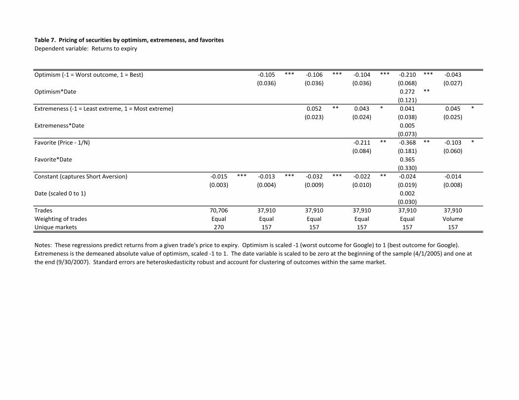
Table 7.  Pricing of securities by optimism, extremeness, and favoritesDependent variable:  Returns to expiry

Optimism (‐1 = Worst outcome, 1 = Best) ‐0.105 *** ‐0.106 *** ‐0.104 *** ‐0.210 *** ‐0.043(0.036) (0.036) (0.036) (0.068) (0.027)

Optimism*Date 0.272 **(0.121)

Extremeness (‐1 = Least extreme, 1 = Most extreme) 0.052 ** 0.043 * 0.041 0.045 *(0.023) (0.024) (0.038) (0.025)

Extremeness*Date 0.005(0.073)

Favorite (Price ‐ 1/N) ‐0.211 ** ‐0.368 ** ‐0.103 *(0.084) (0.181) (0.060)

Favorite*Date 0.365(0.330)

Constant (captures Short Aversion) ‐0.015 *** ‐0.013 *** ‐0.032 *** ‐0.022 ** ‐0.024 ‐0.014(0.003) (0.004) (0.009) (0.010) (0.019) (0.008)

Date (scaled 0 to 1) 0.002(0.030)

Trades 70,706 37,910 37,910 37,910 37,910 37,910Weighting of trades Equal Equal Equal Equal Equal VolumeUnique markets 270 157 157 157 157 157

Notes:  These regressions predict returns from a given trade's price to expiry.  Optimism is scaled ‐1 (worst outcome for Google) to 1 (best outcome for Google).  Extremeness is the demeaned absolute value of optimism, scaled ‐1 to 1.  The date variable is scaled to be zero at the beginning of the sample (4/1/2005) and one at the end (9/30/2007).  Standard errors are heteroskedasticity robust and account for clustering of outcomes within the same market.

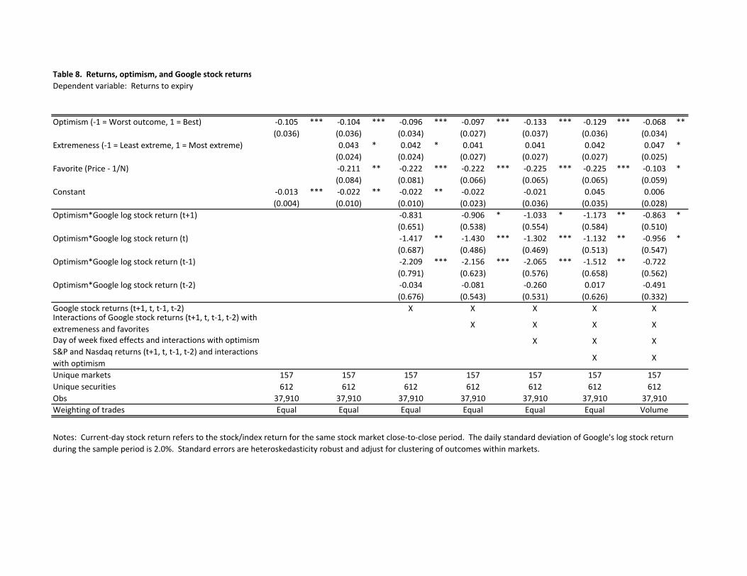
Table 8.  Returns, optimism, and Google stock returnsDependent variable:  Returns to expiry

Optimism (‐1 = Worst outcome, 1 = Best) ‐0.105 *** ‐0.104 *** ‐0.096 *** ‐0.097 *** ‐0.133 *** ‐0.129 *** ‐0.068 **(0.036) (0.036) (0.034) (0.027) (0.037) (0.036) (0.034)

Extremeness (‐1 = Least extreme, 1 = Most extreme) 0.043 * 0.042 * 0.041 0.041 0.042 0.047 *(0.024) (0.024) (0.027) (0.027) (0.027) (0.025)

Favorite (Price ‐ 1/N) ‐0.211 ** ‐0.222 *** ‐0.222 *** ‐0.225 *** ‐0.225 *** ‐0.103 *(0.084) (0.081) (0.066) (0.065) (0.065) (0.059)

Constant ‐0.013 *** ‐0.022 ** ‐0.022 ** ‐0.022 ‐0.021 0.045 0.006(0.004) (0.010) (0.010) (0.023) (0.036) (0.035) (0.028)

Optimism*Google log stock return (t+1) ‐0.831 ‐0.906 * ‐1.033 * ‐1.173 ** ‐0.863 *(0.651) (0.538) (0.554) (0.584) (0.510)

Optimism*Google log stock return (t) ‐1.417 ** ‐1.430 *** ‐1.302 *** ‐1.132 ** ‐0.956 *(0.687) (0.486) (0.469) (0.513) (0.547)

Optimism*Google log stock return (t‐1) ‐2.209 *** ‐2.156 *** ‐2.065 *** ‐1.512 ** ‐0.722(0.791) (0.623) (0.576) (0.658) (0.562)

Optimism*Google log stock return (t‐2) ‐0.034 ‐0.081 ‐0.260 0.017 ‐0.491(0.676) (0.543) (0.531) (0.626) (0.332)

Google stock returns (t+1, t, t‐1, t‐2) X X X X XInteractions of Google stock returns (t+1, t, t‐1, t‐2) with extremeness and favorites X X X X

Day of week fixed effects and interactions with optimism X X XS&P and Nasdaq returns (t+1, t, t‐1, t‐2) and interactions with optimism

X X

Unique markets 157 157 157 157 157 157 157Unique securities 612 612 612 612 612 612 612Obs 37,910 37,910 37,910 37,910 37,910 37,910 37,910Weighting of trades Equal Equal Equal Equal Equal Equal Volume

Notes:  Current‐day stock return refers to the stock/index return for the same stock market close‐to‐close period.  The daily standard deviation of Google's log stock return during the sample period is 2.0%.  Standard errors are heteroskedasticity robust and adjust for clustering of outcomes within markets.

Table 9.  Regressions predicting trade characteristics from traders' attributesDependent variable:  Security characteristic*(1 if buy, ‐1 if sell)

Dependent variableRelationship with returnsCoder?  (Participated in code review) 0.033 ‐0.102 *** ‐0.284 *** ‐0.404 *** 0.072 ***

(0.049) (0.022) (0.081) (0.139) (0.023)Level (Distance from CEO) 0.006 0.004 0.066 ** 0.102 ** 0.023 **

(0.019) (0.007) (0.029) (0.040) (0.009)Hire date (in years) 0.051 ** ‐0.032 *** ‐0.093 *** ‐0.224 *** 0.005

(0.021) (0.008) (0.034) (0.041) (0.009)NYC‐based ‐0.169 ‐0.050 * 0.028 0.014 0.017

(0.105) (0.029) (0.086) (0.121) (0.024)Mountain View (MTV)‐based ‐0.119 ‐0.101 *** 0.161 * ‐0.005 0.045

(0.105) (0.031) (0.096) (0.122) (0.029)Distance to Noname Café in miles (0 if non‐MTV) 0.032 0.085 * ‐0.161 ‐0.597 ** 0.069

(0.125) (0.047) (0.179) (0.294) (0.043)Experience [Ln(1 + previous trades)] ‐0.014 ‐0.044 *** ‐0.049 *** ‐0.094 *** 0.026 ***

(0.011) (0.004) (0.019) (0.031) (0.003)TradesUnique traders

Optimism Favorite Extreme(scaled ‐1 to 1) Price ‐ 1/N Abs(Optimism) Buy Return

Neg. Neg. Pos. Neg.

Note:  Each observation is a side of a trade.  Regressions use trader chatacteristics to predict security characteristics, multipled by ‐1 if the side in question is a sell.  Regressions include trade fixed effects and a dummy variable for one particular extremely prolific trader.  Standard errors are heteroskedasticity robust and adjust for clustering of outcomes within person.

37,910 70,706 37,910 70,706 70,7061,126 1,463 1,126 1,463 1,463

Table 10.  Geography and trading correlationsDependent variable:  net shares purchased (normalized)Independent variables:  Proximity‐weighted normalized sums of colleagues' pre‐trade positions

Geographical proximitySame city 0.006 0.000 0.003 ‐0.001 ‐0.002 ‐0.002

(0.004) (0.006) (0.007) (0.006) (0.006) (0.006)Proximity within city 0.010 * ‐0.004 ‐0.014 * ‐0.014 * ‐0.013    (100ft/distance between buildings, min = 0, max = 1) (0.006) (0.007) (0.008) (0.008) (0.008)Same building 0.022 *** 0.008 ‐0.001 0.002

(0.005) (0.007) (0.007) (0.007)Same floor 0.025 *** ‐0.019 * ‐0.020 *

(0.009) (0.010) (0.010)Proximity on floor  0.090 *** 0.053 ***   (10ft/distance between offices, min = 0, max = 1) (0.015) (0.017)Same office 0.055 ***

(0.016)Building information missing for either party ‐0.004 ‐0.005 0.000 0.000 ‐0.001

(0.005) (0.005) (0.006) (0.006) (0.005)Room information missing for either party ‐0.021 *** ‐0.025 *** ‐0.025 ***

(0.008) (0.008) (0.008)Other controls

Trade fixed effectsInitial position

ObservationsR‐squared

X

Notes:  Independent variables are the sum of the pre‐trade position of a trader's colleagues, weighted by the variable given (e.g., an indicator for whether the two traders are in the same city).  Standard errors are heteroskedasticity robust and adjust for clustering of outcomes within person.

140,768 140,768 140,768 140,768 140,768 140,7680.03990.0352 0.0354 0.0359 0.0378 0.0395

X X X X XX X X X X X

(1) (2) (3) (4) (5) (6)

Table 11.  Social and work relationships and correlated tradingDependent variable:  net shares purchased (normalized)Independent variables:  Proximity‐weighted normalized sums of colleagues' pre‐trade positions

Social connectionsSelf‐reported professional relationship? 0.016 * 0.009 0.010 0.012 0.017 0.020 *

(0.009) (0.009) (0.010) (0.010) (0.011) (0.011)Self‐reported friendship? ‐0.001 ‐0.044 ** ‐0.050 ** ‐0.050 ** ‐0.040 * ‐0.054 **

(0.019) (0.021) (0.020) (0.021) (0.022) (0.023)# of overlapping email lists 0.000 ‐0.001 ‐0.003 ‐0.004 ‐0.005 ‐0.007

(0.003) (0.003) (0.003) (0.003) (0.004) (0.005)Work history

Reviewed each other's code 0.028 *** 0.027 *** 0.019 ** 0.023 ** 0.017 *(0.009) (0.009) (0.009) (0.009) (0.009)

Overlapped on project? 0.034 *** 0.010 ‐0.031 ** ‐0.050 *** ‐0.026(0.012) (0.014) (0.015) (0.016) (0.016)

Organizational proximitySame SVP (one level below CEO) 0.016 *** 0.014 ** 0.015 *** 0.015 **

(0.006) (0.006) (0.006) (0.006)Same "2‐Levels‐below‐CEO" manager ‐0.011 * ‐0.008 ‐0.007 ‐0.007

(0.006) (0.008) (0.008) (0.008)Same "3‐Levels‐below‐CEO" manager 0.033 ** ‐0.018 ‐0.026 ‐0.026

(0.014) (0.017) (0.017) (0.017)1‐2 steps away on org chart 0.102 *** 0.061 *** 0.068 ***

(0.018) (0.017) (0.017)3 steps away on org chart ‐0.016 ‐0.020 * ‐0.019 *

(0.011) (0.011) (0.011)Other controls

Trade fixed effectsInitial positionGeographic proximity variables (from Table 10, cols 6)Demographic similarity

ObservationsR‐squared

XX

Notes:  The last column includes 8 variables capturing the pre‐trade positions of colleagues who are similar along a demographic dimension (attended the same undergraduate school, had the same undergrad major, are both or neither in programming roles at Google, are both native English speakers, share a common non‐English native language, or are similar according to three commonly studied demographic variables).

0.035 0.0357 0.0372 0.0392 0.0423 0.0433

(5)

X

(6)

140,768 140,768 140,768 140,768 140,768 140,768

XXXX

XX XXX X X

(2) (3) (4)

X

(1)

Table 12.  Robustness of the relationship with geographyDependent variable:  net shares purchased (normalized)Independent variables:  Proximity‐weighted normalized sums of colleagues' pre‐trade positions

Geographical proximitySame city ‐0.002 ‐0.001 ‐0.001 0.000 0.004 0.006

(0.006) (0.006) (0.006) (0.006) (0.006) (0.006)Proximity within city ‐0.013 ‐0.015 * ‐0.014 ‐0.015 * ‐0.020 *** ‐0.022 ***    (100ft/distance between buildings, min = 0, max = 1) (0.008) (0.009) (0.009) (0.009) (0.008) (0.008)Same building 0.002 0.004 0.003 0.005 0.003 0.003

(0.007) (0.007) (0.007) (0.007) (0.007) (0.007)Same floor ‐0.020 * ‐0.023 ** ‐0.022 ** ‐0.023 ** ‐0.024 ** ‐0.021 **

(0.010) (0.010) (0.010) (0.010) (0.010) (0.010)Proximity on floor  0.053 *** 0.054 *** 0.052 *** 0.053 *** 0.057 *** 0.049 ***   (10ft/distance between offices, min = 0, max = 1) (0.017) (0.017) (0.018) (0.017) (0.017) (0.018)Same office 0.055 *** 0.093 *** 0.094 *** 0.096 *** 0.097 *** 0.073 ***

(0.016) (0.018) (0.018) (0.019) (0.020) (0.020)Building information missing for either party ‐0.001 ‐0.001 0.001 0.000 0.000 0.000

(0.005) (0.006) (0.006) (0.006) (0.006) (0.006)Room information missing for either party ‐0.025 *** ‐0.025 *** ‐0.025 *** ‐0.025 *** ‐0.025 *** ‐0.023 ***

(0.008) (0.008) (0.008) (0.008) (0.008) (0.008)Organizational proximity

1‐2 steps away on org chart 0.073 ***(0.017)

Other controlsTrade fixed effectsInitial positionDemographic similaritySocial connectionWork historyOrganizational proximity (same 1st, 2nd, and 3rd‐level managers)

ObservationsR‐squared

X

XXXX

X

Notes:  The controls added in successive columns are the proximity‐weighted pre‐trade colleague position variables from Table 11.

X XX

XXX

XX

0.0399 0.0412 0.0414 0.0415 0.0425 0.0432140,768 140,768 140,768 140,768 140,768 140,768

XX X X X X XX X X X X

(6)(1) (2) (3) (4) (5)

Table 13.  Timing of geographical proximity effects Dependent variable:  net shares purchased (normalized)Independent variables:  Proximity‐weighted normalized sums of colleagues' pre‐trade positions

Proximity (beginning of week of trade)Same city ‐0.002 ‐0.028 ‐0.048 0.006 ‐0.018 ‐0.048

(0.006) (0.024) (0.053) (0.006) (0.024) (0.054)Proximity within city ‐0.015 * ‐0.004 0.012 ‐0.022 *** ‐0.009 0.004

(0.008) (0.011) (0.013) (0.008) (0.012) (0.013)Same building 0.001 0.011 0.010 0.003 0.010 0.012

(0.007) (0.009) (0.012) (0.007) (0.009) (0.012)Same floor ‐0.017 ‐0.025 * ‐0.019 ‐0.021 ** ‐0.030 ** ‐0.025

(0.010) (0.013) (0.016) (0.010) (0.013) (0.016)Proximity on floor  0.042 ** 0.012 0.018 0.049 *** 0.018 0.017

(0.018) (0.022) (0.028) (0.018) (0.023) (0.028)Same office 0.035 ** 0.067 ** 0.097 ** 0.073 *** 0.078 ** 0.098 **

(0.017) (0.031) (0.038) (0.020) (0.031) (0.039)1‐2 steps away on org chart 0.031 ** ‐0.009 ‐0.018 0.073 *** 0.023 ‐0.018

(0.012) (0.024) (0.023) (0.017) (0.027) (0.026)Proximity (13 weeks before trade)

Same city 0.028 ‐0.016 0.027 ‐0.015(0.024) (0.026) (0.025) (0.027)

Proximity within city ‐0.016 * ‐0.018 ** ‐0.013 ‐0.016 **(0.009) (0.008) (0.008) (0.008)

Same building ‐0.010 ‐0.011 ‐0.014 ‐0.016(0.011) (0.010) (0.011) (0.010)

Same floor 0.015 0.002 0.017 0.006(0.015) (0.014) (0.014) (0.014)

Proximity on floor  ‐0.046 ‐0.027 ‐0.015 ‐0.004(0.030) (0.029) (0.030) (0.029)

Same office 0.038 * 0.053 ** 0.040 * 0.056 ***(0.022) (0.022) (0.022) (0.022)

1‐2 steps away on org chart 0.046 * 0.041 * 0.058 ** 0.054 **(0.024) (0.021) (0.026) (0.023)

Proximity (13 weeks after trade)Same city 0.067 0.075

(0.046) (0.047)Proximity within city ‐0.003 ‐0.006

(0.011) (0.011)Same building ‐0.008 ‐0.007

(0.011) (0.012)Same floor 0.012 0.012

(0.015) (0.014)Proximity on floor  ‐0.043 ‐0.031

(0.044) (0.045)Same office ‐0.032 ‐0.029

(0.024) (0.024)1‐2 steps away on org chart 0.011 0.031

(0.020) (0.022)Controls

Trade fixed effectsInitial positionSocial, work, org, and demographic variables

ObservationsR‐squared

Notes:  All regressions also include controls for the sum of pre‐trade positions when either building or room information is missing for either party.  Cols 4‐6 include all of the social, organizational, and demographic variables in Table 11.

X X XX X XX X X

140,768 140,768 130,600 130,600

(4) (5) (6)

0.0432 0.0440 0.03330.0408 0.03020.0401140,768 140,768

(1) (2) (3)

X X XX X X

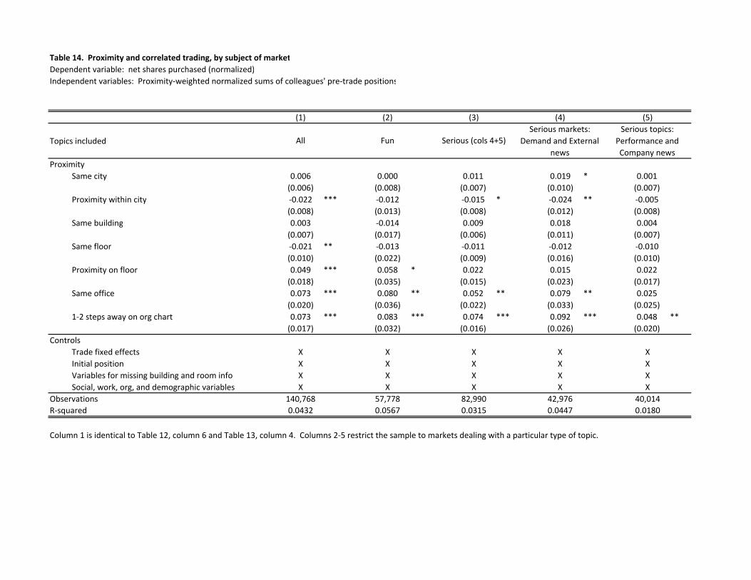
Table 14.  Proximity and correlated trading, by subject of marketDependent variable:  net shares purchased (normalized)Independent variables:  Proximity‐weighted normalized sums of colleagues' pre‐trade positions

Topics included

ProximitySame city 0.006 0.000 0.011 0.019 * 0.001

(0.006) (0.008) (0.007) (0.010) (0.007)Proximity within city ‐0.022 *** ‐0.012 ‐0.015 * ‐0.024 ** ‐0.005

(0.008) (0.013) (0.008) (0.012) (0.008)Same building 0.003 ‐0.014 0.009 0.018 0.004

(0.007) (0.017) (0.006) (0.011) (0.007)Same floor ‐0.021 ** ‐0.013 ‐0.011 ‐0.012 ‐0.010

(0.010) (0.022) (0.009) (0.016) (0.010)Proximity on floor  0.049 *** 0.058 * 0.022 0.015 0.022

(0.018) (0.035) (0.015) (0.023) (0.017)Same office 0.073 *** 0.080 ** 0.052 ** 0.079 ** 0.025

(0.020) (0.036) (0.022) (0.033) (0.025)1‐2 steps away on org chart 0.073 *** 0.083 *** 0.074 *** 0.092 *** 0.048 **

(0.017) (0.032) (0.016) (0.026) (0.020)Controls

Trade fixed effectsInitial positionVariables for missing building and room infoSocial, work, org, and demographic variables

ObservationsR‐squared

42,9760.0447

XX

140,7680.0432

57,7780.0567

82,9900.0315

XXXX

Serious topics:  Performance and Company news

XX

XXXX

XXXX

(4)Serious markets:  

Demand and External news

(5)

Column 1 is identical to Table 12, column 6 and Table 13, column 4.  Columns 2‐5 restrict the sample to markets dealing with a particular type of topic.

0.018040,014

X XXX

(1)

All

(2)

Fun

(3)

Serious (cols 4+5)

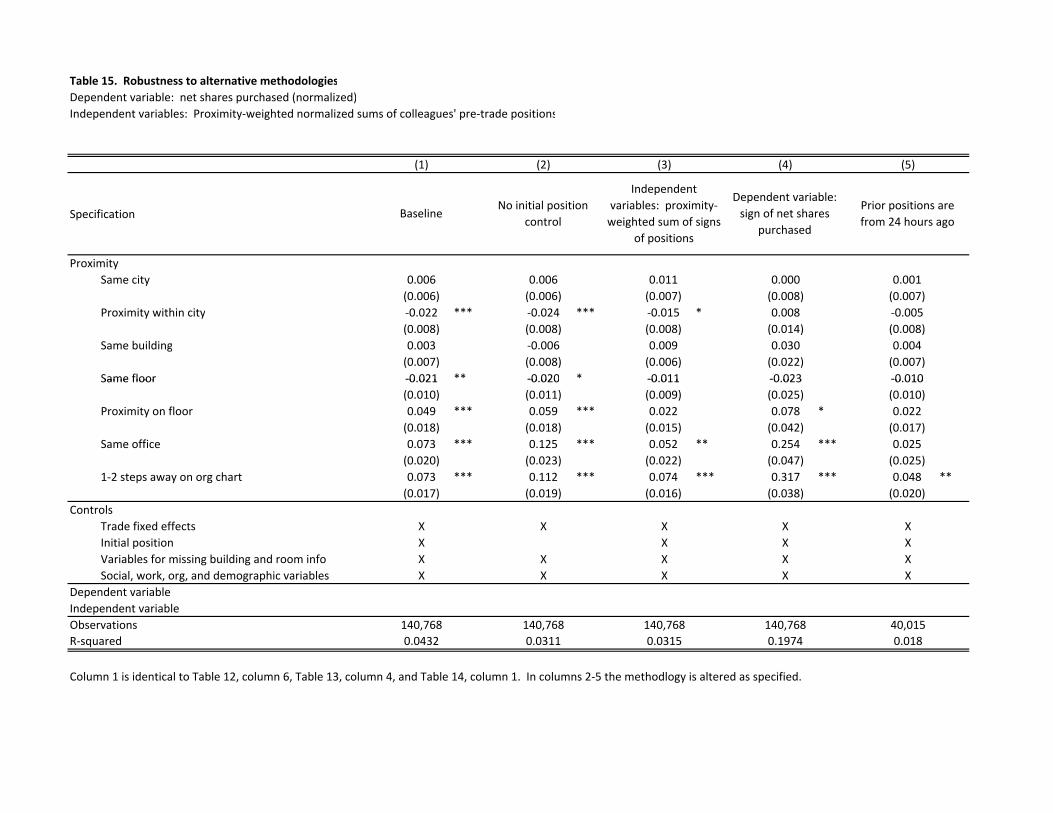
Table 15.  Robustness to alternative methodologiesDependent variable:  net shares purchased (normalized)Independent variables:  Proximity‐weighted normalized sums of colleagues' pre‐trade positions

Specification

ProximitySame city 0.006 0.006 0.011 0.000 0.001

(0.006) (0.006) (0.007) (0.008) (0.007)Proximity within city ‐0.022 *** ‐0.024 *** ‐0.015 * 0.008 ‐0.005

(0.008) (0.008) (0.008) (0.014) (0.008)Same building 0.003 ‐0.006 0.009 0.030 0.004

(0.007) (0.008) (0.006) (0.022) (0.007)Same floor ‐0.021 ** ‐0.020 * ‐0.011 ‐0.023 ‐0.010

(5)

Prior positions are from 24 hours ago

(1) (2) (3) (4)

BaselineNo initial position 

control

Independent variables:  proximity‐weighted sum of signs 

of positions

Dependent variable:  sign of net shares 

purchased

Same floor ‐0.021 ‐0.020 ‐0.011 ‐0.023 ‐0.010(0.010) (0.011) (0.009) (0.025) (0.010)

Proximity on floor  0.049 *** 0.059 *** 0.022 0.078 * 0.022(0.018) (0.018) (0.015) (0.042) (0.017)

Same office 0.073 *** 0.125 *** 0.052 ** 0.254 *** 0.025(0.020) (0.023) (0.022) (0.047) (0.025)

1‐2 steps away on org chart 0.073 *** 0.112 *** 0.074 *** 0.317 *** 0.048 **(0.017) (0.019) (0.016) (0.038) (0.020)

ControlsTrade fixed effectsInitial positionVariables for missing building and room infoSocial, work, org, and demographic variables

Dependent variableIndependent variableObservationsR‐squared

Column 1 is identical to Table 12, column 6, Table 13, column 4, and Table 14, column 1.  In columns 2‐5 the methodlogy is altered as specified.

XXXX

40,0150.018

140,768 140,768 140,768 140,7680.0432 0.0311 0.0315 0.1974

X X X XX X X X

X X X XX X X