Using Operational Planning Horizons for

Determining Setup Changes

RAHUL DE'

Bowie State University, Bowie, MD, USA

JERROLD H MAY

University of Pittsburgh, Pittsburgh, PA, USA

(Received October 1996; accepted after revision December 1997)

We consider operational planning horizons required for managing shop ¯oor resources. Our conceptof horizons is di�erent from those developed in the literature for aggregate production planning; thefocus is on operational-level decisions. Our problem is of scheduling machine setup changes and weconduct the study on a system implemented at a manufacturing facility. This system schedules ma-chine setup changes at a particular stage of manufacturing.We identify a horizon parameter, l,which impacts the number of setup changes made. Short horizons increase the number of setupchanges while reducing the work-in-process, whereas long horizons reduce the setups while increas-ing the work-in-process. We develop a metric for assessing the setup change schedules made by thesystem and use this to show that l is related to certain shop ¯oor characteristics. We conclude thatthese characteristics should be used to determine l. # 1998 Elsevier Science Ltd. All rightsreserved

Key wordsÐscheduling, horizons, decision support systems, operations management

1. INTRODUCTION

OPERATIONAL PLANNING HORIZONS are usedimplicitly by many decision makers who areworking in a dynamic operations environment.However, this parameter is not explicitly used asa decision parameter in the research literaturein operations management. This paper makesa case for the explicit consideration of oper-ational planning horizons for managing shop¯oors. The case is built up with evidence froman implementation of a simple machine setupscheduling system at a Westinghouse manufac-turing plant. The system assists a scheduler inmaking setup change decisions and explicitlyemploys a parameter for the determination ofthe operational planning horizon.

Operational planning horizons (OPHs) di�erfrom the traditional notions of planning hor-izons in the durations of time concerned andthe level, and scope, of decision making. As

the name suggests, OPHs deal with the oper-

ational level of decision making. This level

entails short time frames and the scope of

analysis is concerned with operational details. In

a manufacturing setting, such details deal with

process times of machines, processing steps,

build-up of queues, setup changes of ma-

chines, etc. The decisions pertain to scheduling

and dispatching the various machines and jobs.

Researchers commenting on the general pro-

blem of building scheduling systems have

pointed out the need to clearly identify a hor-

izon for which plans or schedules have to be

made. To quote Rickel [10]: ``The importance

of determining the correct scheduling horizon

cannot be overemphasized. . . .The horizon

should be chosen based on properties of the

plant, the machines, and the orders''. McKay

et al. point out the problems that appear if

horizons are arbitrarily selected [7]: `` . . . the

Omega, Int. J. Mgmt Sci. Vol. 26, No. 5, pp. 581±592, 1998# 1998 Elsevier Science Ltd. All rights reserved

Printed in Great Britain0305-0483/98 $19.00+0.00PII: S0305-0483(98)00001-2

581

ripple e�ect of one bad scheduling decisionlasts for a long time''. Thus, on a dynamicshop ¯oor, their study of scheduling and sche-dulers showed, it is best to assign resourcesbased on a time horizon determined from theexisting conditions.

Historically, planning horizons for manufac-turing have referred to horizons for aggregateplans. The problems focus on ®nding theperiod of time, the horizon, for which pro-duction should be scheduled, whether such aperiod exists, or establishing the parametersrelevant to ®nding such horizons. In mostcases the horizons are established by examin-ing the tradeo�s involved in incurring certaintypes of costs, such as inventory carrying costsversus setup costs, etc. (This research is exam-ined in more detail later.)

In this paper we focus on OPHs and theiruse within systems that support scheduling de-cisions. We begin with a discussion of a setupchange scheduling problem at a manufacturingfacility. We, brie¯y, describe a system that wasbuilt to address this problem. This discussionpoints to the need for OPHs and the par-ameters that can be used for them. We showwhy an arbitrary selection of a value for thisparameter would be counter-productive. Then,we describe a number of experiments to ident-ify the properties of OPHs and examine howshop ¯oor characteristics can be used to estab-lish the horizon. (The phrase scheduling hor-izon has also been used for the same idea. We,however, persist with using operational plan-ning horizon in order to semantically associateit with decision making levels.)

2. SCHEDULING PROBLEM

We motivate the discussion about OPHs bystudying a problem of real-life shop ¯oor sche-duling. The site for this study is the Westing-house Nuclear Fuels Division Specialty MetalsPlant, in Blairsville, Pennsylvania. The pro-blem deals with the issue of reassigning ma-chines, already assigned to various productgroups, by executing setup changes at requiredtimes. Figure 1 shows the schematic of a gen-eral machine assignment situation on a shop¯oor. Four machine groups are shown, whereall the machines in one group have the samesetup. Each machine group is processing jobsbelonging to one product, thus, the con®gur-

ation shows four products (A, B, C and D)being processed currently. These machines areat the same stage of the manufacturing processand the time required to process each job inthe di�erent product lines is (approximately) thesame. The machines can be switched betweendi�erent product groups by changing their set-ups. The queues in front of the machinegroups indicate the number of jobs awaitingprocessing. The circles indicate the jobs.

The problem of determining machine setupchanges arises if there are not enough jobsavailable to keep all the machines running, fora given time period, in a particular machinegroup. A machine from this group can thus bemoved to some other group, if there is a need.One example of this is Group 3 which is pro-cessing product C. If, simultaneously, there isanother group in which a machine is short,owing to a large queue of jobs waiting to beprocessed, as in Group 1, then a setup changecan be executed to move a machine fromGroup 3 to Group 1. On the other hand, ifthe load on Group 1 is temporary, not likelyto last for any signi®cant length of time, andthe lull in the tra�c of materials arriving atGroup 3 is also temporary, then it would notbe judicious to execute the setup change.

The problem is limited by certain conditionspertaining to the shop ¯oor: (1) the number ofmachines available to this stage of processingis ®nite and limited; (2) the setup changes areexpensive. Each setup change requires at least30% of the time required to process one job.These conditions ensure that setup changes arenot arbitrarily executed and have to beplanned for in advance. The cost of the setupchange is determined by the cost of the diesthat have to be changed and the productivityloss due to down time of the machine. Also,the machines have to be quality tested for pro-duction, and there is a cost for running samplejobs and testing them; (3) the demand for theproducts is known. The ``pull'' created on theproducts is determined by the demand.

3. SYSTEM DESIGN AND IMPLEMENTATION

A system was designed to suggest solutionsfor the setup change problems outlined above.The system, called the PLANOPTICON, wasbased on scheduling knowledge obtained froman expert scheduler and was implemented at

De', MayÐUsing Operational Planning with Setup Changes582

the Westinghouse plant. An explicit objectiveof the system was to encode the heuristics eli-cited from the scheduler, enabling it to per-form the scheduling tasks in a manner similarto that of the human expert. This system wasbuilt as part of a larger project to build acomprehensive shop ¯oor management system.

A team of researchers, including theauthors, started looking at the problem ofdesigning a shop ¯oor planning and schedul-ing system in the fall of 1989. Several monthswere spent working with a scheduler, a personwho had spent over thirty years with theplant, in order to understand the planning andscheduling system in place. An importantobjective was to elicit some of the schedulingheuristics that the scheduler used. Over thenext few years several systems were designedand tested [6], one of which wasPLANOPTICON [2].

PLANOPTICON was a knowledge-basedsystem, was written in Lisp and ran on aWindows-based personal computer. The sys-tem was implemented at the Westinghousefacility and was thoroughly validated. Its de-cisions were compared with the scheduler's de-cisions for the same input conditions, andstatistical tests showed its performance to bevery accurate for certain horizon levels [2].

Recently, the Westinghouse management re-engineered their production processes with sig-ni®cant changes in their operational par-ameters. Thus, the system is currently notbeing used.

The system based decisions about machinesetup changes principally on projections ofqueues. From the current status of the shop¯oor the queues were projected for n periodsinto the future (i.e. for n periods the net sizeof the queue was forecast). Once the queuesizes were available, they were compared tothe desired range of values for the queue. Fromthis it was decided whether a setup changewas required, either to add a machine to a lineor remove one, and the period at which thisshould be done. For example, in Fig. 1, if it isnoticed that line A is consistently heavy formore than two (or any number l) periods, sayfor periods t to t + l, and the line C is consist-ently light, a decision about moving a machineover from C to A can be made, at period t.

The projections are then recast from timet + 1 with the change in the status of the pro-

duct lines included in the new forecast. Thisforms the second set of projections. Again, thedecisions about heavy or light queues aremade and setup changes are scheduled. Theprocess of projecting queues, making decisionsabout machine setup changes, executing thechanges, and re-projecting continues until thequeue sizes are all within the ranges speci®edfor the n time periods for which the projec-tions are done. The schedules for the machinesetup changes are now the setup changes thatwere made to average out the queues.

The queue projections are made by addingto the queue the number of jobs that areexpected to arrive in the next period and sub-tracting from it those that will be consumedby the machines. To estimate the jobs that canarrive at the queue, all the possible jobs in agiven product line in previous stages are con-sidered and probability estimates are used tocompute whether they will arrive at the queue.The probabilities are based on observed beha-vior on the shop ¯oor. The estimates of con-sumption are based on average performanceof the machines. Sizes of the queues are thusprojected for the di�erent product lines. Newjobs that are introduced on the shop ¯oor inthe current time period are also steppedthrough in a similar manner. (Further detailsabout the system are provided in [2].)

4. DETERMINATION OF PARAMETER ``L''

The parameter n speci®es the number ofperiods for which the simulations are made.The parameter l speci®es the number ofperiods to look ahead to decide on the sizes ofqueues. What should be the sizes of n and l?Clearly, n should be as large as the demanddata available can support it to be. If there issu�cient (demand) data available, we need avalue of n that will, at least, allow the systemto step the jobs currently in backstream pro-cesses to complete through this stage. n willthus be determined by the situation at a par-ticular site. (If there is no demand data avail-able then the projections would be based onforecasted demand.)

We assume a value of n(=10) for our situ-ation that meets the above criteria.

The value of l, however, poses certain pro-blems. l is used to detect changes in the sizesof the queues which are then used to decide

Omega, Vol. 26, No. 5 583

on the machine setup changes. If the queuesare very small and l is set to a value muchhigher than required to process the queues onthe available machines, then the system willwait l periods before it recognizes the di�er-ence and schedules setup changes. If thequeues are heavy and l is set to a small value,then the system will be su�ciently sensitive tothe evolving situation. This scenario suggests asmall value of l.

Now, consider a situation where a queue issmall, l is set to a small value, and after abrief lull the queue builds up again (because,say, a load from back stream processes arrivesat the queue.) In this case, owing to the smallvalue of l, the system will respond rapidly bymoving machines away from the machinegroup and will then bring them back when thenew jobs arrive; overlooking the obviouspossibility of waiting for the new jobs. With ahigh enough value of l, this problem would beresolved.

Clearly, the value of l has to be some aver-age between the very near-sighted and the veryfar-sighted values. We postulate that l has tobe estimated empirically by considering thecharacteristics of the shop ¯oor. This postulateis also based on the fact that analytical modelsavailable in the literature are not applicable in

this situation. To elaborate this latter opinionwe brie¯y consider the literature.

5. LITERATURE REVIEW

The role of horizons in decision making hasbeen studied by many researchers. In a classicstudy of the cognitive activities invoked forplanning daily chores, Hayes-Roth and Hayes-Roth [4] establish that the times for the begin-ning of events and the duration of activitiesare crucial to the planning task. They are themarkers around which reasoning about theactions to be performed occur. The planneralso implicitly works with a temporal horizon,which in some cases becomes explicit. In therealm of formal decision making, it has beenshown that horizon considerations have a de®-nite impact on the planning process. (Weassume that planning is also a decision makingactivity.) The work of Kotteman and Remus[5] shows clearly that horizon considerationsimpact the planning process and in some casesimprove on it. They force planners to locatetheir reasoning around the assumed or com-puted horizon.

The literature in management science con-siders the issues in selecting horizons quiteextensively. These horizons are developed for

Fig. 1. The scheduling problem: machine groups and product queues. The circles indicate jobs awaitingprocessing, and the squares indicate machines in each group

De', MayÐUsing Operational Planning with Setup Changes584

aggregate plans or for capacity expansion.Some of the ideas are brie¯y reviewed here.

In the domain of aggregate planning thenotion of a production horizon is associatedwith the optimal or lowest cost productionplan [12]. A production plan determines thequantities of goods to produce in any pro-duction period, given the data about demandand costs. The costs primarily relate to setupcosts required to produce the goods and thecosts of holding inventory. An optimal planwould recommend the quantities of goods toproduce or store in inventories in di�erentperiods, which would minimize the costs andat the same time meet the demand. The under-lying tradeo�s are of costs of producing or ofstoring. In extreme situations, say where thesetup costs is very high and the storing cost isnegligible, it would be optimal to produce forall periods in the initial period itself and holdinventories, whereas if the cost of storage isvery high as compared to the cost of setupsthen it would be advantageous to produce thegoods only in accordance with the demand ineach period. Typically, a production planwould suggest a strategy in between the twoextremes, where goods would be produced forsome periods and held for some periods.

The idea of horizons, the manner in whichit is understood and computed, has subtlevariations in the literature. Wagner andWhitin [13] consider a horizon as a number ofperiods for which an optimal plan is available.The duration of the horizon is broken up intosuccessive intervals for which goods are pro-duced and held in inventory. A similar notionis employed by Modigliani and Hohn [8].

Morton [9] considers only the optimal de-cision for the ®rst period and here the horizonis the number of periods for which the compu-tations have to be done to ®nd the best costsolution for the ®rst interval. The algorithmused to compute the plans need only considerthe data for the duration of the horizon to®nd the optimal solution for the ®rst interval.Bean and Smith [1] follow a similar idea of ahorizon. They de®ne two horizon parameterswhich are used in the domain of capacity plan-ning: (1) a forecast horizon, which is the num-ber of periods to consider for the ®rst periodoptimal plan; and (2) a decision horizon,which is the duration of the ®rst decision, orthe time until the next decision.

The principal inputs to the Wagner andWhitin algorithm, and other algorithms, arethe demand, the cost of setups and the cost ofcarrying inventory for each period. For theoperational planning situation considered inthis paper, the inputs are the number of jobsin backstream processes,the number of ma-chine groups, the number of machines in eachgroup, the queue loads in front of each group,and the demand, speci®ed in terms of jobsentered into the system. The algorithms fromthe literature do not deal with the level ofdetail used at the operational level. Even if thedata were somehow modi®ed and ®tted into aWagner and Whitin type of algorithm and anoutput is obtained, we would miss out ondetails such as: the number of machines thatneed to be changed in each interval; the inter-vals in which the setups have to be changed;the interchanges between machine groups thatwould be required.

Thus, at an aggregate level a productionplan may be obtained by directly applying analgorithm developed in the literature, but atthe level of operational planning, where detailsare important, this approach is not acceptable.Our argument for the empirical estimation ofhorizon parameters is thus supported.

6. EXPERIMENTS, DATA AND RESULTS

We have conducted a series of experimentswith data obtained from the Westinghouseplant. Our experiments had three objectives:(1) establish whether the horizon parameterhas any e�ect on the schedules created for ma-chine setup changes; (2) identify the set of pro-cess descriptors that have a bearing ondetermining the values of the horizon par-ameter l; (3) identify the range of values forthe process descriptors that determine the``best'' value for l.

The inputs to the system consist of dailysnapshots of the shop ¯oor (Table 1), anddemand information. The snapshot depicts,for each product, the total number of jobs inthe previous stages, the number of jobsassigned to machines, and the number of jobsin the queues. (The demand here is indicatedby the total number of new jobs started for ntime periods.) The system uses this infor-mation to forecast the future possible snap-shots, or projections. The output from the

Omega, Vol. 26, No. 5 585

system is a set of schedules for setup changesat di�erent time periods (Table 2). (The``Index'' in Table 2 refers to time periods.)Each schedule indicates the number of ma-chines that have to be changed along with thesource and target product groups for di�erentindices.

We ran 68 randomly selected snapshotsthrough the system and obtained schedules fordi�erent values of the horizon parameter l. Weused 0, 2, 4, 6, 8 and 10, as di�erent levels of lto assess if these would have any e�ect on theschedules produced by the system.

One clear di�erence in the schedules pro-duced by the system, for di�erent levels of l, isin the number of changes suggested. For 68snapshots, we counted the number of changesscheduled, for the ®rst three periods, for indi-ces 0, 1 and 2 (index 0 or time period 0 standsfor the snapshot that is used for the projec-tions) and found that:

(1) Using the analysis of variance tech-nique, we found the di�erencesamongst the sample means to be sig-ni®cant (at 1% level). A plot of theaverage number of changes scheduledfor di�erent l levels is shown in Fig. 2.

These results show that for lower values of l,i.e. for shorter look-ahead levels, the system is``myopic'' and tries to address all the queueimbalances immediately, resulting in the highernumber of setup changes scheduled. Theresults also suggest that to keep setup changesat a minimum one has to simply select a high

value of l, where the changes are the least.However, this would be a hasty conclusion, asother parameters are not considered.

Consider the build-up of queues in front ofthe fourth stage machines; it is higher forhigher values of l (Fig. 3). The di�erences inqueue build-ups between all four l levels is sig-ni®cant (using analysis of variance, at 1%level). For high l levels, say l8, the systemwaits for a heavy or light load to hold for 8time periods before it schedules changes toaddress this. In doing so it allows the queuesto build up to high values.

Thus, there is a trade-o� involved in select-ing the value of l. For lower l, setup changesare greater but queues are smaller, whereas forhigher l, it is vice versa. This suggests thatthere is a ``best'' or optimal level of l.

7. EMPIRICAL ESTIMATION OF L

We turn to the problem of estimating l. Ourapproach is to run statistical tests to identifywhether there are a set of shop ¯oor par-ameters that can be used to ®nd a value for l.Then, we de®ne and use a metric to assess theschedules produced by the system for di�erentlevels of l. We use the same metric to identifythe relationship of l with signi®cant shop ¯oorparameters.

Our approach is exploratory; we will show afeasible method by which the horizon par-ameter can be estimated. Although this is nota standard or complete methodology, we pre-sent this to raise issues for both constructionof, and research on, scheduling systems. Onehundred and three (103) snapshots were runthrough the system for ®ve di�erent horizon

Fig. 2. Average number of machine setup changes for 68randomly selected snapshots. The setup changes, on thevertical axis, are shown for di�erent horizon levels, on the

horizontal axis

Table 1. An example of a snapshot. Cell values are num-ber of jobs

TIME-INDEX: t

Product Stage 1 Stage 2 Stage 3 Stage 4 QStage4 M

A 0 2 7 9 4B 1 8 7 1 5C 6 2 0 8 3

Legend: Q= Number of jobs in the queue; M=Numberof jobs on machines

Table 2. Output from the system

Move From To At Index

2 Machines Product B Product C 11 Machine Product D Product E 3* * * *

De', MayÐUsing Operational Planning with Setup Changes586

levels (l0 is being excluded from this analysis).This generated 515 di�erent data points. Eachdata point consisted of ®ve ®elds, which are:

(1) The dependent variable, denoting thenumber of setup changes planned.

(2) The planning horizon, i.e. l.(3) D, the demand, denoting the total

number of jobs applied in a ®ve-dayperiod (for all products). This variablehas seven levels, where each level cor-responds to a range (<20, 20±24,etc.). (We use ranges to restrict thenumber of levels.)

(4) P, the total number of products onthe shop ¯oor at the beginning of theprojections. This variable also hasseven levels going from 3 to 9.

(5) Pnew, the number of new productsthat are added during the projections.Each product would have a certainnumber of jobs. This parameter indi-cates the number of new productsthat didn't already exist on the shop¯oor, and are added afresh during thecourse of the simulation.

The data was analyzed with the GeneralLinear Models (analysis of variance) pro-cedure of SAS. The output revealed that l, P,Pnew have a signi®cant impact on the numberof setup changes scheduled. The demand, D,does not have a signi®cant impact on thenumber of setup changes. (Details of theanalysis are provided in Appendix A.) Thefact that the horizon parameter l has a signi®-cant e�ect on the dependent variable was alsoestablished in the earlier results. From the cur-rent analysis, the most important result is that

the number of products, P, and the number of

new products, Pnew, have a signi®cant impact

on the dependent variable. This result can be

explained by the fact that setup changes are

principally planned for exchanges between

products, so ¯uctuations in the number of

products on the shop ¯oor signi®cantly impact

the number of changes.

The demand, by itself, does not have a sig-

ni®cant impact on the dependent variable. The

reason is that the e�ect of the variations in the

load is not felt for the n periods for which the

analysis is being done. Note that, our initial

rationale for not selecting the algorithms from

literature, used for computing aggregate plan-

ning horizons, is justi®ed by this result.

To determine a relationship between the fac-

tors l and P, we use the same data as that gen-

erated for the previous analysisÐoutput for

®ve levels of l and 103 input data snapshots.

The ®rst set of analyses concerns a compari-

son of the plans made by the system with

those made by the scheduler, for the same

starting snapshot, on the shop ¯oor.

The standard by which the performance of

the system is measured is a historical record.

The historical record is a collection of snap-

shots obtained from the factory. The schedule

of machine setup changes proposed by the sys-

tem, for a particular snapshot date, is com-

pared with the historical record, for the same

date, of actual machine setup changes that

were made on the shop ¯oor.

We feel that a historical record is an appro-

priate measure for the performance of the sys-

tem because the system, as was mentioned in

Section 3, was designed to explicitly encode

Fig. 3. Average sizes of queues for 10 randomly selected snapshots. The vertical axis shows the totalnumber of jobs in the queue for di�erent horizon levels. The horizontal axis shows the number of

periods, or indices, for which the projections are done

Omega, Vol. 26, No. 5 587

the heuristics of the human scheduler. In thisregard, the best performance that the systemcould achieve would be one as close to that ofthe scheduler's as possible. The historicalrecord re¯ects, primarily, the scheduler's de-cisions. It also includes decisions made byshop supervisors, who made contingency de-cisions above those made by the scheduler.Although it is possible to use other metrics tomeasure the performance of the schedules gen-erated by the system, a number of which arediscussed in [3], we focus on a comparisonwith the historical record. There are tworeasons for this: (1) the multiple objectives forscheduling setup changes, such as reducingqueue sizes (the WIP) or maximizing machineutilization, are included within the decisionsmade by the scheduler; and (2) the systemfocuses on decisions at a particular stage ofthe manufacturing process, thus, studying theimpact of its decisions on aggregate par-ameters, such as work-in-process or cycle time,is not an accurate measure of its performance.

The manner in which the plans made by thesystem are compared to the historical record isas follows: each snapshot for which plans arecomputed by the system is given an index of 0(the system produces plans for indices 0through n). The historical record is consultedand setup changes in the snapshots of datescorresponding to the indices 0 through n arerecorded. The successes and errors are countedas follows:

(1) If a plan is made by the system toadd or remove a machine to a pro-duct line in periods 0, 1, or 2, and amachine was actually added to orremoved from the particular productline in either of the dates correspond-ing to periods 0, 1, or 2, then this iscounted as a success.

(2) If a plan is made to add or removefrom a particular product line inperiods 0, 1, or 2, and this is not actu-ally executed in the dates correspond-ing to 0, 1, or 2, then this is countedas an error of ``Type A''.

(3) If an actual execution of a setupchange took place in periods 0, 1, or2, and a corresponding addition orremoval was not planned for by thesystem in any of the three periods,

then this is counted as an error of

``Type B''. (Type A errors are thus

errors of ``commission'' and Type B

errors are errors of ``omission''.)

We chose two additional snapshots, indices 1

and 2, by which to compare the performance

of the system with the historical record

because setup changes planned by the schedu-

ler were not always executed on the same day.

For example, if the scheduler marked a setup

change on the snapshot of index 0, and this

was, say, a Monday, then this change could

appear in the revised snapshot of Monday

itself, or of Tuesday if it was executed later in

the day on Monday or early on Tuesday. If it

was executed after Tuesday's snapshot was

®nalized, then it would appear on the snap-

shot of Wednesday.

A plot of the successes, Type A errors and

Type B errors depicted in Fig. 4, shows that

as the horizon level increases, the numbers for

successes and Type A errors decrease. If the

net value of the successes is considered (where

the Type A errors are subtracted from the suc-

cesses) then a ``best'' value is obtained at level

l4. This net value is an indicator of the per-

formance of the system at a particular horizon

level.

Type B errors increase as the level of l

increases. As was shown earlier the total num-

ber of setups decreases as l increases (the sys-

tem is ``lethargic''). For higher levels of l, the

resulting lower number of setups increases the

chance of Type B errors whereas the chances

of Type A errors are reduced; and the reverse

happens at lower levels of l. Considering the

sum of both types of errors, the total number

is lowest at l4.

The patterns for the overall successes and

errors with respect to the levels of l could be

further explained by an analysis of the success

rates with regard to the process characteristics.

As was shown earlier, the number of products

on the shop ¯oor has a signi®cant impact on

the number of setups. To examine the e�ect

this factor has on the success-rate, we would

have to consider the e�ect of the various levels

of the number of products.

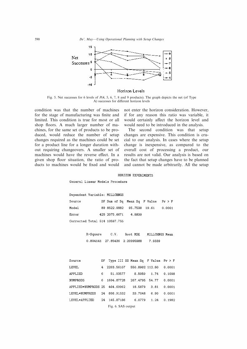
A plot of the totals for successes and errors

for all the levels of the number of products is

shown in Fig. 5.

De', MayÐUsing Operational Planning with Setup Changes588

From Fig. 5 it will be seen that for a largenumber of products, e.g. 9, lower values of thenet success-rate are obtained for larger valuesof l, and, the net success-rate is greater whenthe length of the horizon is short. As the num-ber of products goes down to 4 or 5 the netsuccess-rate for horizon levels of 4 and 6increases and exceeds those for 2. The success-rate increases as the number of productsdecreases and as the horizon length increases.The impact of the number of products and lon the net success-rate is depicted in Table 3.

Thus, the relation between the number of pro-ducts on the shop ¯oor and the horizon length isinverse, as far as creating the ``best'' plans isconcerned. As the number of productsincreases, it is better to reduce the length ofthe horizon parameter l. Conversely, as thenumber of products reduces, it is better toincrease the horizon length.

8. CONCLUSIONS

We make our case for operational planninghorizons: the horizon parameter l signi®cantlyimpacts setup change decisions, that is, thenumber of setup changes scheduled. A shorthorizon makes the system very sensitive toqueue size changes, and it tends to addressthis with many setup changes. A long horizon

makes the system ``lethargic'' and it tends tomake fewer setup changes which drives up thequeue loads. The latter is a problem as itincreases the overall work-in-process loads onthe entire production system.

A statistical analysis showed us that theplanned setup changes are in¯uenced by thehorizon parameter, the number of products onthe shop ¯oor and new products introduced.The setup changes are not a�ected by theaggregate demand.

Using historical data obtained from theshop ¯oor we devised a metric for assessingthe schedules produced by the system. Thisprovided us with a tool to measure the per-formance of the system at di�erent horizonlevels. The metric used the following conceptsof performance: successes, for those schedulesthat match the historical record; errors, forthose that did not. From the sample of datawe used, l4 turned out to have the best netsuccess values.

By employing the same metric we relatedthe number of products on the shop ¯oor withl and found that they were inversely related.Fewer products require less exchanges of ma-chines, thus allowing longer horizons. Moreproducts require a greater number of machineexchanges, consequently requiring short hor-izons.

Our results can be formulated in a generalway as follows: the system makes decisionsabout shop ¯oor resourcesÐmachinesÐbymonitoring certain eventsÐqueue sizes. Theduration for which the monitoring is done isused as the operational horizon parameter.Shorter and longer durations have di�erentconsequences on the decisions being made.

With the growing emphasis on computer-integrated manufacturing and intelligent sche-duling of shop ¯oor resources, it is imperativethat key decisions on the shop ¯oor be ident-i®ed and horizon parameters and their valuesbe estimated accurately. Our results show thataggregate parameters like demand do not havea role to play in these situations. Instead, wecan usefully rely on shop ¯oor parameterssuch as the number of products to identify thebest values for the horizons.

We had stated in the description of the pro-blem that our study was limited by certainconditions of the particular shop ¯oor fromwhere we had collected our data. The ®rst

Table 3. Impact of l and number of products on net suc-cesses

l

Number of products High Low

High lesser greaterLow greater lesser

Fig. 4. Successes and errors. Net values are computed bysubtracting errors (Type A or Type B) from the successes.

Summarized for 34 randomly selected snapshots

Omega, Vol. 26, No. 5 589

condition was that the number of machinesfor the stage of manufacturing was ®nite andlimited. This condition is true for most or allshop ¯oors. A much larger number of ma-chines, for the same set of products to be pro-duced, would reduce the number of setupchanges required as the machines could be setfor a product line for a longer duration with-out requiring changeovers. A smaller set ofmachines would have the reverse e�ect. In agiven shop ¯oor situation, the ratio of pro-ducts to machines would be ®xed and would

not enter the horizon consideration. However,if for any reason this ratio was variable, itwould certainly a�ect the horizon level andwould need to be introduced in the analysis.

The second condition was that setupchanges are expensive. This condition is cru-cial to our analysis. In cases where the setupchange is inexpensive, as compared to theoverall cost of processing a product, ourresults are not valid. Our analysis is based onthe fact that setup changes have to be plannedand cannot be made arbitrarily. All the setup

Fig. 6. SAS output

Fig. 5. Net successes for 6 levels of P(4, 5, 6, 7, 8 and 9 products). The graph depicts the net (of TypeA) successes for di�erent horizon levels

De', MayÐUsing Operational Planning with Setup Changes590

changes do not have to be of the same type,that is, they could take di�ering amounts oftime or resources for di�erent products andmachines. This also implies that the machinesdo not all have to be of the same type. Wemade this assumption initially to simplify ourproblem (see Fig. 1).

The third condition was that the demandwas known. This condition is required toensure that we can run the simulations to cre-ate the snapshot projections. In light of ouranalysis it is clear that the demand infor-mation is not needed for computing the hor-

izon values. This condition, thus, does notdetract from the generalizability of our results.

We had also simpli®ed the problem by con-sidering a situation in which all the machineswere at the same stage of processing. This wasa practical consideration, deployed in order tolimit the scope of the system. A stage at theWestinghouse plant was distinguished fromanother on the basis of the time it took toprocess the jobs. For instance, we focused onstage four where the jobs were processed in1.6 times the amount of time it took to pro-cess them in stage three. There would be varia-

Fig. 7. SAS outputÐwith four factors

Omega, Vol. 26, No. 5 591

bility in processing times for di�erent productson di�erent machines within each stage, butall the processing times would remain with10±15% of the average processing time. Ourresults for the horizon level are only valid forstage four. We would have to compute thehorizon level separately for stage three or anyother stage in the plant. (We focused on stagefour because these were, usually, the bottle-neck machines.)

This simpli®cation does limit the generaliz-ability of our results. However, we hope toinclude the e�ect of varying process times onthe horizon parameter in future research.

ACKNOWLEDGEMENTS

This research has been funded, in part by a grant from theUniversity Research Council, Western Illinois University.We are grateful to our anonymous reviewers for manyuseful suggestions.

APPENDIX

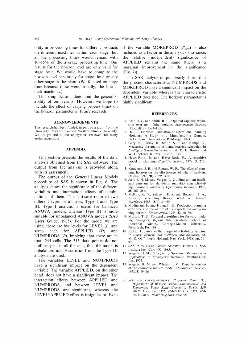
This section presents the results of the dataanalysis obtained from the SAS software. Theoutput from the analysis is provided alongwith its assessment.

The output of the General Linear Modelsprocedure of SAS is shown in Fig. 6. Theanalysis shows the signi®cance of the di�erentvariables and interaction e�ects of combi-nations of them. The software reported twodi�erent types of analysis, Type I and TypeIII. Type I analysis is useful for balancedANOVA models, whereas Type III is moresuitable for unbalanced ANOVA models (SASUsers Guide, 1985). For the model we areusing, there are ®ve levels for LEVEL (l), andseven each for APPLIED (D) andNUMPRODS (P), implying that there are intotal 245 cells. The 515 data points do notuniformly ®ll in all the cells, thus the model isunbalanced and F-statistics from the Type IIIanalysis are used.

The variables LEVEL and NUMPRODShave a signi®cant impact on the dependentvariable. The variable APPLIED, on the otherhand, does not have a signi®cant impact. Theinteraction e�ects between APPLIED andNUMPRODS, and between LEVEL andNUMPRODS are signi®cant, whereas theLEVEL*APPLIED e�ect is insigni®cant. Even

if the variable MOREPROD (Pnew) is alsoincluded as a factor in the analysis of variance,the relative (independent) signi®cance ofAPPLIED remains the same (there is amarginal improvement in the signi®cance(Fig. 7)).

The SAS analysis output clearly shows thatthe process characteristics NUMPRODS andMOREPROD have a signi®cant impact on thedependent variable whereas the characteristicAPPLIED does not. The horizon parameter ishighly signi®cant.

REFERENCES

1. Bean, J. C. and Smith, R. L., Optimal capacity expan-sion over an in®nite horizon. Management Science,1985, 31(12), 1523±1532.

2. De', R., Empirical Estimation of Operational PlanningHorizons: A Study in a Manufacturing Domain,Ph.D. thesis, University of Pittsburgh, 1993.

3. Gary, K., Uzsoy, R., Smith, S. P. and Kempf, K.,Measuring the quality of manufacturing schedules. InIntelligent Scheduling Systems, ed. D. E. Brown andW. T. Scherer. Kluwer, Boston, 1995.

4. Hayes-Roth, B. and Hayes-Roth, F., A cognitivemodel of planning. Cognitive Science, 1979, 3, 275±310.

5. Kotteman, J. E. and Remus, W. E., The e�ect of plan-ning horizon on the e�ectiveness of what-if analysis.Omega, 1992, 20(3), 295±301.

6. Jerrold, H. M. and Vargas, L. G., Simpson: an intelli-gent assistant for short-term manufacturing schedul-ing. European Journal of Operational Research, 1996,88, 269±286.

7. McKay, K. N., Safayeni, F. R. and Buzacott, J. A.,Job-shop scheduling theory: What is relevant?Interfaces, 1988, 18(4), 84±90.

8. Modigliani, F. and Hohn, F. E., Production planningover time and the nature of the expectation and plan-ning horizon. Econometrica, 1955, 23, 46±66.

9. Morton, T. E., Forward algorithms for forward-think-ing managers, Reprint 966, Graduate School ofIndustrial Admin., Carnegie-Mellon University,Pittsburgh, PA, 1981.

10. Rickel, J., Issues in the design of scheduling systems.In Expert Systems and Intelligent Manufacturing, ed.M. D. Oli�. North Holland, New York, 1988, pp. 70±89.

11. SAS, SAS Users' Guide: Statistics Version 5. SASInstitute Inc., Cary NC, 1985.

12. Wagner, H. M., Principles of Operations Research withApplications to Managerial Decisions. Prentice-Hall,Inc., 1975.

13. Wagner, H. M. and Whitin, T. M., Dynamic versionof the economic lot size model. Management Science,1958, 5, 89±96.

ADDRESS FOR CORRESPONDENCE: Professor Rahul De',Department of Business, Public Administration andEconomics, Bowie State University, Bowie, MD20715, USA. Tel: (301) 464-7737; Fax: (301) 464-7873; Email: Rahul.De@bowiestate.edu.

De', MayÐUsing Operational Planning with Setup Changes592