Using Numerical Bifurcation Analysis to Study Pattern ... · J.A. Sherratt Pattern Formation in...

Heriot-Watt University Research Gateway

Heriot-Watt University

Using Numerical Bifurcation Analysis to Study Pattern Formation in Mussel BedsSherratt, Jonathan Adam

Published in:Mathematical Modelling of Natural Phenomena

DOI:10.1051/mmnp/201611506

Publication date:2016

Document VersionPeer reviewed version

Link to publication in Heriot-Watt University Research Portal

Citation for published version (APA):Sherratt, J. A. (2016). Using Numerical Bifurcation Analysis to Study Pattern Formation in Mussel Beds.Mathematical Modelling of Natural Phenomena, 11(5), 86-102. DOI: 10.1051/mmnp/201611506

General rightsCopyright and moral rights for the publications made accessible in the public portal are retained by the authors and/or other copyright ownersand it is a condition of accessing publications that users recognise and abide by the legal requirements associated with these rights.

If you believe that this document breaches copyright please contact us providing details, and we will remove access to the work immediatelyand investigate your claim.

https://doi.org/10.1051/mmnp/201611506

https://pureapps2.hw.ac.uk/portal/en/publications/using-numerical-bifurcation-analysis-to-study-pattern-formation-in-mussel-beds(1f86f96e-8e6f-4459-9607-33327edbc694).html

Download date: 28. Jul. 2018

Math. Model. Nat. Phenom.

Vol. ?, No. ?, 2016, pp. ?-?

Using Numerical Bifurcation Analysis to Study

Pattern Formation in Mussel Beds

J.A. Sherratta 1

a Department of Mathematics and Maxwell Institute for Mathematical Sciences,

Heriot-Watt University, Edinburgh EH14 4AS, UK

Abstract. Soft-bottomed mussel beds provide an important example of ecosystem-scale self-

organisation. Field data from some intertidal regions shows banded patterns of mussels, running

parallel to the shore. This paper demonstrates the use of numerical bifurcation methods to investi-

gate in detail the predictions made by mathematical models concerning these patterns. The paper

focusses on the “sediment accumulation model” proposed by Liu et al (Proc. R. Soc. Lond. B 14

(2012), 20120157). The author calculates the parameter region in which patterns exist, and the

sub-region in which these patterns are stable as solutions of the original model. He then shows

how his results can be used to explain numerical observations of history-dependent wavelength

selection as parameters are varied slowly.

Key words: mussels, pattern formation, periodic travelling wave, reaction-diffusion-advection,

numerical continuation, wavetrain

AMS subject classification: 92B05, 92D40, 35M10

1 Introduction

Pattern formation at the scale of whole ecosystems is an active sub-discipline within spatial ecol-

ogy. There are now many examples of such landscape-scale patterns, and mathematical modelling

1E-mail: [email protected]

1

J.A. Sherratt Pattern Formation in Mussel Beds

is playing a key role in understanding them because the opportunities for empirical study are typ-

ically very limited. Examples include banded vegetation on semi-arid hillslopes [7, 37, 43], “fairy

circles” in Namibia [56], patterns of ridges and hollows in peatlands [13, 14], “ribbon forests” in

the Rocky mountains [1], localised patches of trees in savannah grasslands [20,46], intertidal mud-

flats [54], and banded patterns in soft-bottomed mussel beds [16, 23, 49]. This paper concerns the

last of these examples. It has long been known that mussels tend to self-organise into patches on

rocky shores [21, 27, 55]. However, larger scale striped patterns have been reported more recently

for mussel beds in both the Dutch Wadden Sea [49] and the Menai Strait (UK) [16]. These are

soft-bottomed systems meaning that the mussels adhere only to one another or to debris such as

shell fragments. They are also intertidal, and the mussel bands are orthogonal to the tidal flow,

with a wavelength of several metres.

Two different mechanisms have been proposed for banded patterns in soft-bottomed mussel

beds. One is the “reduced losses” hypothesis, which was due originally to van de Koppel et al [49].

Mussel beds are subject to disruption by predation, wave action, and ice scouring [12]. These

pressures are resisted by the attachment of mussels to one another, via byssal threads. More of

these attachments form when the mussels are subject to perturbations [52]. Therefore van de

Koppel et al [49] hypothesised that the per capita loss rate of mussels will be reduced at higher

mussel densities. This is consistent with empirical data showing that mussel density increases in

response to both greater wave exposure [48] and greater predation threat [5, 26]. A mathematical

model based on the reduced losses hypothesis was originally proposed by van de Koppel et al [49]

and has been studied and modified in a number of subsequent papers [3, 17, 22, 35, 53].

The focus of this paper is the alternative “sediment accumulation” hypothesis proposed by

Liu et al [22]. Being filter feeders mussels produce sediment (pseudo-faeces), and in the context

of a mussel bed this can significantly affect the topography – thus mussels are “ecosystem engi-

neers” [15,51]. For a substrate with hummocks and troughs, hydrodynamics implies that the water

velocity will be greater at a hummock than at a trough, and Liu et al [22] hypothesised that this

will increase the supply rate of algae, which is the main food source for mussels in these ecosys-

tems. This is consistent with empirical data, also in [22], revealing a positive correlation between

elevation and mussel density. Since larger mussel densities imply more rapid sediment deposition,

this hypothesis sets up a positive feedback loop that has the potential to generate patterns.

2 The sediment accumulation model

Liu et al [22] proposed a mathematical model based on their “sediment accumulation” hypothesis,

formulated in terms of algal density a(x, t), mussel density m(x, t) and the amount of accumulated

sediment s(x, t):

2


∂a/∂t =

transfer to/from upperwater layers︷︸︸︷1− αa −

depth-dependentconsumptionby mussels︷︸︸︷

βam(s+ η)/(s+ 1)+

advectionby tide︷︸︸︷

ν ∂a/∂x (2.1)

∂m/∂t =

musselgrowth︷︸︸︷

δam(s+ η)/(s+ 1)−

death︷︸︸︷m +

randommovement︷︸︸︷∂2m/∂x2 (2.2)

∂s/∂t = m︸︷︷︸production

− θs︸︷︷︸erosion

+D∂2s/∂x2

︸︷︷︸dispersal

. (2.3)

This is a dimensionless version of the model: details of the dimensional version and the nondimen-

sionalisation are given in [22]. The spatial coordinate x increases with distance from the shore; tdenotes time, and α, β, δ, θ, η < 1, ν and D are positive parameters. The only nonlinear terms

in the model are the mussel growth rate δam(s + η)/(s + 1) and the corresponding rate of algal

consumption: per capita growth is an increasing function of both algal density and the amount of

sediment. This nonlinearity provides a short-range activation of mussel density, and the advection

of algae from the open sea generates long-range inhibition, because the mussels compete spatially

for food. Together these processes can lead to pattern formation, and a typical pattern solution is

illustrated in Figure 1.

An important prelude to the study of patterns in (2.1–2.3) is to calculate the homogeneous

steady states. For all parameter values there is a mussel-free steady state (a,m, s) = (1/α, 0, 0).Steady states with a non-zero mussel density require a sufficiently high level of algal supply, specif-

ically

δ ≥ δcrit ≡

[α− βθη +

(4αβθ(1− η)

)1/2].

Then there are two other steady states, (a,m, s) =(a±, m±, s±

)where

a± = (s± + 1)/[δ(s± + η)

](2.4)

m± = θs± (2.5)

s± =1

2βθ

[δ − α− βθη ±

{(δ − α− βθη)2 − 4βθ(α− δη)

}1/2]. (2.6)

General conditions on the stability of these steady states are very complicated, but for parameter

values given by the estimates of Liu et al [22] (1/α, 0, 0) and (a+, m+, s+) are stable to spatially

homogeneous perturbations, while (a−, m−, s−) is unstable [22].

Pattern solutions of (2.1–2.3) move away from the shore, as shown in Figure 1. Intuitively

this is because the model predicts higher algal densities on the off-shore side of a mussel band

compared to the on-shore side, due to consumption in the band, and this causes a net growth

of mussels on the off-shore side and a net loss on the on-shore side. This results in a gradual

net off-shore migration. Mathematically the movement is a consequence of the advection term,

which means that pattern onset occurs via a Turing-Hopf rather than a Turing bifurcation [24,

28, 31]. In fact, there is no evidence of large scale migration of banded patterns in real mussel

3


Figure 1: An illustration of a patterned solution of the model (1). The solution is plotted at t = 500, 502and 504; the arrows show the direction of pattern movement, which is in the positive x direction, i.e. away

from the shore. The equations were solved using a semi-implicit finite difference scheme on a domain of

length 50 with periodic boundary conditions. The initial condition was a small perturbation to the uniform

steady state (a+,m+, s+), with the perturbation consisting of a sum of small-amplitude sine functions of

period 50/N , N = 1, . . . , 10. The parameters were α = 50, β = 200, δ = 320, η = 0.1, ν = 360, θ = 2.5,

D = 1.

4


beds. A natural explanation for this is the oscillatory nature of tidal flow, which would imply

bidirectional oscillating advection of algae rather than the unidirectional term in (2.1). This has

been investigated recently for an alternative model of banded pattern formation [39], showing that

bidirectional advection can generate patterns that do not show large scale migration. However for

mathematical simplicity we restrict attention in this paper to the unidirectional advection case.

Since pattern solutions of (2.1–2.3) move with constant shape and speed, they are periodic

travelling waves: a(x, t) = a(z), m(x, t) = m(z) and s(x, t) = s(z) where z = x−ct. Here c > 0is the migration speed. Solutions of this form satisfy the ordinary differential equations

(ν + c) ∂a/∂z + 1− αa− β am(s+ η)/(s+ 1) = 0 (2.7)

∂2m/∂z2 + c ∂m/∂z + δ am(s+ η)/(s+ 1)− m = 0 (2.8)

D∂2s/∂z2 + c ∂s/∂z + m− θs = 0 (2.9)

with patterns corresponding to limit cycle solutions. The key ecological control parameter is δ,

which reflects the algal concentration in the upper water layers, and I consider changes in δ with

the other ecological parameters fixed; I take the fixed values from Liu et al (2012). However while

varying δ one must also consider changes in the wave speed c, which is an additional parameter

introduced by the travelling wave ansatz. Therefore my initial aim is to determine the part of the

δ–c plane in which there are patterns (i.e. periodic travelling waves, or equivalently limit cycle

solutions of (2.7–2.9)).

3 The parameter regions giving patterns

A useful first step in calculating the parameter region giving patterns is to construct bifurcation

diagrams for the equations (2.7–2.9) as δ is varied with c fixed. The starting point for the bifurca-

tion diagrams is the steady state (a, m, s) = (a+, m+, s+) since this corresponds to a steady state

of (2.1–2.3) that is stable to spatially homogeneous perturbations: one expects patterns to develop

when it becomes unstable to spatially inhomogeneous perturbations. An example bifurcation dia-

gram is shown in Figure 2. At large values of δ there are no patterns, but as δ is decreased there

is a Hopf bifurcation in (2.7–2.9) from which a branch of limit cycle (pattern) solutions emanates.

This solution branch terminates at a homoclinic point, meaning that the period of the limit cycle

tends to infinity; thus as δ is decreased towards this point the mussels bands become more and

more widely separated. For values of the speed c close to that used in Figure 2 it is the loci of the

Hopf bifurcation and homoclinic point that enclose the region of the δ-c parameter plane giving

patterns.

The simple form of the bifurcation diagram in Figure 2 does not apply for all values of c:two complications can arise. First, the branch of pattern solutions may have a fold, rather than

proceeding monotonically from the Hopf bifurcation to the homoclinic point (e.g. Figure 3). In

some parts of the δ–c parameter plane the locus of this fold forms one boundary of the parameter

region giving patterns. Note that in general, for any system of ODEs, the part of a parameter

plane in which limit cycles exist is bounded by segments of three types of loci: Hopf bifurcations,

homoclinic points, and folds in a limit cycle solution branch.

5


0

0.1

0.2

0.3

0.4

0.5

0.6

0.7

0.8

0.9

250 260 270 280 290 300 310 320 330

Mea

n of

M

delta

Figure 2: Bifurcation diagram for (2.7–2.9) showing the mean mussel density as a function of δ with the mi-

gration speed c = 0.6. The other parameters are α = 50, β = 200, η = 0.1, ν = 360, θ = 2.5, D = 1. The

square indicates a Hopf bifurcation point, and the open circle indicates a homoclinic point. All calculations

and plotting were done using the software package WAVETRAIN (www.ma.hw.ac.uk/wavetrain)

[34, 36]. Full details of the WAVETRAIN input files, run commands and plot commands are given at

www.ma.hw.ac.uk/∼jas/supplements/mmnp-bif/.

0

0.1

0.2

0.3

0.4

0.5

0.6

0.7

0.8

0.9

305 310 315 320 325 330

Mea

n of

M

delta

Figure 3: Bifurcation diagram for (2.7–2.9) showing the mean mussel density as a function of δ with

the migration speed c = 1.2. The other parameters are as in Figure 2. The square indicates a Hopf

bifurcation point, the open circle indicates a homoclinic point, and the closed circle indicates a fold in

the solution branch. All calculations and plotting were done using the software package WAVETRAIN

(www.ma.hw.ac.uk/wavetrain) [34, 36]. Full details of the WAVETRAIN input files, run commands

and plot commands are given at www.ma.hw.ac.uk/∼jas/supplements/mmnp-bif/.

6


0

0.1

0.2

0.3

0.4

0.5

0.6

0.7

0.8

322 324 326 328 330 332

Mea

n of

M

delta

Figure 4: Bifurcation diagram for (2.7–2.9) showing the mean mussel density as a function of δwith the migration speed c = 1.375. The other parameters are as in Figure 2. The square in-

dicates a Hopf bifurcation point and the open circles indicates homoclinic points. All calculations




The other potential complication is that there may be a second, disconnected branch of patterns

(e.g. Figure 4). This solution branch does not arise from a Hopf bifurcation point in (2.7–2.9):

rather, it connects two different homoclinic points. In some parts of the parameter plane it is loci

of these homoclinic points that form the boundary of the parameter region giving patterns.

I calculated these various loci using WAVETRAIN [34] (www.ma.hw.ac.uk/wavetrain);

the result is shown in Figure 5. WAVETRAIN is a software package specifically designed for the

study of periodic travelling wave solutions of partial differential equations. It determines the loci by

numerical continuation, for which it uses the software package AUTO [8–10]. WAVETRAIN is also

able to determine whether the patterns are stable as solutions of the original model (2.1–2.3), via

numerical continuation of the essential spectrum: this methodology was originally developed by

Rademacher and coworkers [30]. Boundaries in the parameter plane between stable and unstable

waves can also be traced, by numerical continuation of special points in the spectrum [30,36]. The

subdivision between stable and unstable patterns is also shown in Figure 5; note that the region

of parameter space giving stable patterns is sometimes known as the Busse balloon [2]. There are

stable patterns for 244.0 < δ < 334.7, and for any δ within this range there is a stable pattern

for a range of values of the migration speed c. There are also unstable patterns for a range of

migration speed values, and in some cases these ranges overlap, implying the coexistence of stable

and unstable patterns with the same migration speed. Note that the stability of periodic travelling

wave solutions of PDEs is determined entirely by the continuous part of the spectrum (the essential

spectrum): there is no point spectrum [32, §3.4.2]. Changes in stability can be either of Eckhaus

(sideband) or Hopf type [29, 36]. In the former case there is a change in the sign of the curvature

7


0.5

1

1.5

2

240 260 280 300 320 340

c

delta

Hopf bifurcation locusHomoclinic solution locusStability boundary (Eckhaus type)Locus of folds

One soln, stable

One soln, unstable

Two solns, one stable, one unstable

Two solns, both unstable

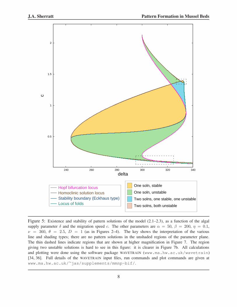
Figure 5: Existence and stability of pattern solutions of the model (2.1–2.3), as a function of the algal

supply parameter δ and the migration speed c. The other parameters are α = 50, β = 200, η = 0.1,

ν = 360, θ = 2.5, D = 1 (as in Figures 2–4). The key shows the interpretation of the various

line and shading types; there are no pattern solutions in the unshaded regions of the parameter plane.

The thin dashed lines indicate regions that are shown at higher magnification in Figure 7. The region

giving two unstable solutions is hard to see in this figure: it is clearer in Figure 7b. All calculations




8


of the spectrum at the origin, while in the latter a fold in the spectrum crosses the imaginary axis at

a point away from the origin; note that the spectrum always passes through the origin because the

patterns are neutrally stable to translations. Investigation of the spectrum, again using WAVETRAIN,

shows that in this case the stability change is of Eckhaus type (Figure 6).

The plot in Figure 5 is particularly complicated in the vicinity of the small “loop” in the homo-

clinic locus, which is shown at greater magnification in Figure 7a. To provide a clearer account of

the behaviour in this part of the parameter plane, Figure 8 shows a series of bifurcation diagrams,

which plot the period of patterns as a function of δ for various fixed values of the migration speed

c. This shows that the solution branch inside the “loop” connects two different homoclinic points,

as in Figure 4, and is separate from that emanating from the Hopf bifurcation point. All patterns

on this separate solution branch are stable as solutions of the model equations (2.1–2.3). Figure 9

shows bifurcation diagrams in which the period of patterns is plotted as a function of c for δ = 328and 332. For these values of δ there are Hopf bifurcations at three different values of c. The speed

c increases monotonically along the solution branch emanating from the largest of these values,

until a homoclinic point is reached. Patterns on this branch are unstable as PDE solutions. For the

middle Hopf bifurcation value, the solution branch also proceeds in the direction of increasing c,and again terminates at a homoclinic solution. Patterns on this branch are initially unstable, with a

switch to stability part way along the branch. On the solution branch emanating from the smallest

of the three Hopf bifurcation points (not shown in Figure 9), c initially decreases before a fold is

reached, after which c increases up to a homoclinic end point. This is illustrated in Figure 7b by

the magnified plot of this part of the δ–c parameter plane. Note that the fold in the Hopf bifurcation

locus at c ≈ 0.2 and δ = 300 corresponds to a transition from Hopf bifurcations of (a+, m+, s+) to

those of (a−, m−, s−); for the parameter values used in the figure, δcrit = 300. Since (a−, m−, s−)is unstable in (2.1–2.3) to even spatially uniform perturbations, one expects intuitively that this

instability will be inherited by the bifurcating patterns, and indeed all patterns in the part of the

parameter plane with c < 0.2 are unstable as PDE solutions.

4 History-dependent changes in pattern wavelength

A good illustration of the value of detailed results on the existence and stability of patterns, such as

is provided by Figure 5, is given by studying the changes in pattern form as a parameter is varied

slowly. Since we used the algal supply level δ as the main control parameter in §3, I consider

slow changes in this parameter. A typical result is illustrated in Figure 10a. I selected a starting

value of δ and used WAVETRAIN to calculate a pattern with a particular wavelength; for Figure 10

I started at δ = 310 with a pattern of wavelength 15. I then decreased δ in small steps, solving for

a fixed (and relatively long) time at each δ value. Note that I did not alter the solution in any way

when changing δ: the numerical results show in Figure 10a are of a single very long numerical

simulation. As δ is decreased the patterns initially retain the same wavelength – though of course

the form of the pattern changes to reflect the new parameter value. One can see this in Figure 10a

because the dots denoting the numerical model solutions lie on the contour of constant pattern

period. However at δ ≈ 290 the period contour leaves the parameter region in which patterns

9


-0.3

-0.2

-0.1

0

0.1

0.2

0.3

-0.7 -0.6 -0.5 -0.4 -0.3 -0.2 -0.1 0 0.1

Im(e

igen

valu

e)

Re(eigenvalue)

(a)

-0.3

-0.2

-0.1

0

0.1

0.2

0.3

-0.7 -0.6 -0.5 -0.4 -0.3 -0.2 -0.1 0 0.1

Im(e

igen

valu

e)

Re(eigenvalue)

(b)

Figure 6: The essential spectra of two pattern solutions of (2.1–2.3), for δ = 280 and (a) c = 0.6, (b)

c = 0.4 with other parameter values as in Figure 5. These parameter values lie either side of the stability

boundary (see Figure 5) and comparison of (a) and (b) shows that the stability change is of Eckhaus type,

meaning that there is a change in the sign of the curvature of the spectrum at the origin. All calculations




10


1.34

1.35

1.36

1.37

1.38

1.39

1.4

1.41

1.42

328 329 330 331 332 333 334

c

delta

alpha=50 beta=200 eta=0.1 nu=360 theta=2.5 D=1

(a)

0.06

0.08

0.1

0.12

0.14

0.16

0.18

290 300 310 320 330

c

delta


(b)

Figure 7: Details of two parts of the δ–c parameter plane, showing the existence and stability of pat-

tern solutions of the model (2.1–2.3). The two regions are indicated by thin dashed lines in Figure 5,

and the values of the other parameters and the interpretation of the various line and shading types are

as in that figure. All calculations and plotting were done using the software package WAVETRAIN



11


20

30

40

50

60

70

80

90

316 318 320 322 324 326 328 330 332 334

perio

d


20

30

40

50

60

70

80

90

316 318 320 322 324 326 328 330 332 334

perio

d


c=1.4

(a)

20

30

40

50

60

70

80

90

316 318 320 322 324 326 328 330 332 334

perio

d


20

30

40

50

60

70

80

90

316 318 320 322 324 326 328 330 332 334

perio

d


c=1.39

20

30

40

50

60

70

80

90

316 318 320 322 324 326 328 330 332 334

perio

d


c=1.39

(b)

20

30

40

50

60

70

80

90

316 318 320 322 324 326 328 330 332 334

perio

dalpha=50 beta=200 eta=0.1 nu=360 theta=2.5 D=1

20

30

40

50

60

70

80

90

316 318 320 322 324 326 328 330 332 334

perio


c=1.375

20

30

40

50

60

70

80

90

316 318 320 322 324 326 328 330 332 334

perio


c=1.375

(c)

20

30

40

50

60

70

80

90

316 318 320 322 324 326 328 330 332 334

perio

d


20

30

40

50

60

70

80

90

316 318 320 322 324 326 328 330 332 334

perio

d


c=1.362

20

30

40

50

60

70

80

90

316 318 320 322 324 326 328 330 332 334

perio

d


c=1.362

(d)

20

30

40

50

60

70

80

90

316 318 320 322 324 326 328 330 332 334

perio

d


20

30

40

50

60

70

80

90

316 318 320 322 324 326 328 330 332 334

perio

d


c=1.361

20

30

40

50

60

70

80

90

316 318 320 322 324 326 328 330 332 334

perio

d


c=1.361

(e)

20

30

40

50

60

70

80

90

316 318 320 322 324 326 328 330 332 334

perio

d


20

30

40

50

60

70

80

90

316 318 320 322 324 326 328 330 332 334

perio

d


c=1.35

20

30

40

50

60

70

80

90

316 318 320 322 324 326 328 330 332 334

perio

d


c=1.35

(f)

20

30

40

50

60

70

80

90

316 318 320 322 324 326 328 330 332 334

perio

d

delta


20

30

40

50

60

70

80

90

316 318 320 322 324 326 328 330 332 334

perio

d

delta


c=1.3

20

30

40

50

60

70

80

90

316 318 320 322 324 326 328 330 332 334

perio

d

delta


c=1.3

(g)

Figure 8: Caption on next page.

12


Figure 8: (Figure on previous page). Bifurcation diagrams for (2.7–2.9) showing the period of pattern

solutions as a function of the algal supply parameter δ. The different panels correspond to different fixed

values of the migration speed c; the other parameters are as in Figure 5. The squares indicate Hopf bifur-

cation points and the circles indicate folds in the solution branch. Lines with dots indicate patterns that are

stable as solutions of (2.1–2.3); lines without dots indicate unstable patterns. These plots should be viewed

in parallel with Figure 7a. All calculations and plots were done using the software package WAVETRAIN



0

10

20

30

40

50

60

70

0.6 0.7 0.8 0.9 1 1.1 1.2 1.3 1.4

perio

d


0

10

20

30

40

50

60

70

0.6 0.7 0.8 0.9 1 1.1 1.2 1.3 1.4

perio

d


delta=328

0

10

20

30

40

50

60

70

0.6 0.7 0.8 0.9 1 1.1 1.2 1.3 1.4

perio

d


delta=328

0

10

20

30

40

50

60

70

0.6 0.7 0.8 0.9 1 1.1 1.2 1.3 1.4

perio

d


delta=328

(a)

0

10

20

30

40

50

60

70

0.6 0.7 0.8 0.9 1 1.1 1.2 1.3 1.4

perio

d

c


0

10

20

30

40

50

60

70

0.6 0.7 0.8 0.9 1 1.1 1.2 1.3 1.4

perio

d

c


delta=332

0

10

20

30

40

50

60

70

0.6 0.7 0.8 0.9 1 1.1 1.2 1.3 1.4

perio

d

c


delta=332

0

10

20

30

40

50

60

70

0.6 0.7 0.8 0.9 1 1.1 1.2 1.3 1.4

perio

d

c


delta=332

(b)

Figure 9: Bifurcation diagrams for (2.7–2.9) showing the period of pattern solutions as a function of the mi-

gration speed c. The two panels correspond to different fixed values of the algal supply parameter δ; the other

parameters are as in Figure 5. The squares indicate Hopf bifurcation points. Lines with dots indicate pat-

terns that are stable as solutions of (2.1–2.3); lines without dots indicate unstable patterns. The dashed lines

indicate the values of c at which the stability boundary crosses the two values of δ. These plots should be

viewed in parallel with Figures 5 and 7a. All calculations and plotting were done using the software package

WAVETRAIN (www.ma.hw.ac.uk/wavetrain) [34,36]. Full details of the WAVETRAIN input files, run

commands and plot commands are given at www.ma.hw.ac.uk/∼jas/supplements/mmnp-bif/.

13


are stable as solutions of (2.1–2.3), and the observed period changes to 20. When δ reaches 274(chosen arbitrarily) I reversed the direction of change and increased δ, in the same small steps. The

pattern remains of period 20: thus there is hysteresis (history dependence) in pattern wavelength.

In Figure 10a the time spent at each δ value is very long (2000 dimensionless units). Figure 10b

shows the corresponding result when this time is halved. In this case the transition to the new

wavelength does not occur until there have been two subsequent decreases in δ. Halving the time

again (to 500 dimensionless units) results in δ reaching the minimum value of 274, starting to

increase again, and then re-entering the region in which the pattern of wavelength 15 is stable, all

before the transition to a longer wavelength would have occurred: hence the pattern remains of

wavelength 15 and there is no hysteresis. Note that the results shown in Figure 10 rely heavily

on the accuracy of my numerical solutions. Therefore in the Appendix I present the results of

convergence tests of my numerical method, which is a simple finite difference scheme. On the

basis of these tests, I fixed the spatial grid spacing at 0.025, with a time step of 5.56× 10−5; these

imply a CFL number of 0.8, and give an error of about 0.03% in the solution (see Table A.1).

History-dependence of pattern wavelength, such as that illustrated in Figure 10a,b, is not a

new result for patterned ecosystems. Similar behaviour has been demonstrated both for models of

semi-arid vegetation [35,43] and for models of soft-bottomed mussels beds based on the “reduced

losses” hypothesis [35]. Its occurrence in this additional case of Liu et al’s model of the “sediment

accumulation” hypothesis for soft-bottomed mussel beds gives an increased sense that such hys-

teresis may be a widespread feature within patterned ecosystems. The practical applications of this

are significant: parameter estimation alone is not enough to predict pattern wavelength, however

carefully it is done. In addition, one requires detailed data on past values of the wavelength.

14


Figure 10: Changes in patterns in the model (2.1–2.3) for sediment-driven mussel bed patterns as the algal

supply parameter δ is varied slowly, with parameter values as in Figure 5, on a domain of length 300. I

decreased δ from 310 to 274 in steps of 9, and then increased it again. The length of (dimensionless)

time spent at each δ value was (a) 2000; (b) 1000; (c) 500. There is no resetting of initial conditions

when δ is changed, and the results in the each part of the figure are for a single long simulation. The

boundary conditions are periodic, and the initial condition is the pattern of wavelength 15 for δ = 310,

which I calculated using WAVETRAIN [34]. The dots show the wavelength and speed immediately before

each change in δ; the arrows indicate the direction in which δ is changing. In (a) the solution follows the

wavelength 15 contour until this leaves the parameter region giving stable patterns, when there is a transition

to the new wavelength of 20. In (b) the behaviour is similar although the change in δ is sufficiently rapid

that the transition to the new wavelength does not occur until there have been two subsequent decreases in

δ. In (c), δ is changed sufficiently fast that it has re-entered the region in which the pattern of wavelength 15is stable before the transition to a longer wavelength would have occurred: hence the pattern remains of

wavelength 15 and there is no hysteresis. Details of the numerical method are given in the Appendix.

Readers considering reproducing this figure should note that the simulation in parts (a), (b) and (c) took

about 18, 9 and 4.5 days respectively on a Linux PC with a 2.83GHz Intel Core 2 Quad Q9500 processor.

15


5 Discussion

Numerical bifurcation analysis is a powerful tool for understanding patterned solutions of partial

differential equations. In this paper I have used it to study Liu et al’s [22] model (2.1–2.3) of the

“sediment accumulation” hypothesis for pattern formation in soft-bottomed mussel beds. Adopting

the implementation of numerical bifurcation analysis in the software package WAVETRAIN [34,36],

I have been able to unravel the complicated dependence on parameter values of pattern existence

and stability; this includes multiple coexisting patterns and disconnected branches of pattern solu-

tions. The most important aspect of the results is the calculation of the region of parameter space

in which there are stable patterns, sometimes known as the Busse balloon [2]. As an illustration

of the value of this calculation, I showed that it enables one to understand the jumps in pattern

wavelength and its history-dependence as a parameter value is varied slowly.

Although my results on pattern existence and stability are detailed, they are not exhaustive,

and (at least) two important features remain to be explored. The first is stability in two space

dimensions. My designation of patterns as stable or unstable refers to their stability in the one-

dimensional PDE system (2.1–2.3). In reality mussel beds occupy a two-dimensional domain, and

although the patterns themselves are one-dimensional (striped patterns) they could be unstable to

perturbations along the stripes (transverse perturbations) even when they are stable as solutions of

(2.1–2.3), i.e. stable to perturbations orthogonal to the stripes. Calculation of stability to transverse

perturbations is more difficult than for one-dimensional perturbations: it is outside the scope of

the software package WAVETRAIN, and to my knowledge there is only one published paper that

calculates this type of stability, namely [42]. In that paper, Siero and coworkers used numerical

bifurcation analysis to calculate the spectrum of striped patterns to transverse perturbations for

the Klausmeier-Gray-Scott model, which has been well studied in the context of applications to

chemistry [4, 11, 18] and semi-arid vegetation [19, 38, 50]. They showed that the parameter region

giving patterns that are stable in one space dimension subdivides, with some of these patterns being

stable to transverse perturbations while others are unstable. The break-up of unstable patterns tends

to generate two-dimensional patterns with a rhombic geometry. Application of Siero et al’s [42]

approach is a natural direction for future work on the model (2.1–2.3) since it would add a new

level of detail that would be necessary for the proper interpretation of two-dimensional numerical

simulation results.

A second aspect of pattern existence and stability that I have not explored is absolute stability.

In any spatiotemporal system, unstable solutions may be either absolutely unstable, or convectively

unstable but absolutely stable. In the latter case, perturbations applied to the solution will grow but

at the same time they will move away from the original site of the perturbation: typically the grow-

ing perturbation eventually reaches a boundary and is then lost. By contrast, “absolute instability”

means that perturbations grow at their original location. (See [33, 41] for full discussions). Any

solution that is not absolutely unstable can be an important long-term component of a solution of

a PDE model, even if it is (convectively) unstable [6, 25, 40, 44]. Therefore it would be extremely

valuable to subdivide the parameter region giving unstable patterns according to whether or not

the patterns are absolutely unstable. However current numerical methods for calculating absolute

stability are either too laborious to be practical in the context of a parameter plane (e.g. [47]) or

16


only apply to spatially uniform solutions [30,45]. The development of new methods for calculating

absolute stability that would enable subdivision of the parameter region giving unstable patterns

for a model such as (2.1–2.3) is a natural but very challenging area for future research.

Appendix: Error estimation for numerical simulations

The calculations in §4 depend heavily on numerical simulations of (2.1–2.3), and therefore a de-

tailed estimation of numerical errors is essential. My numerical scheme is of a simple finite dif-

ference type, with diffusion terms evaluated semi-implicitly, an explicit upwinding representation

of advection, and explicit evaluation of the reaction terms. I used a uniform grid spacing ∆x and

time step ∆t. Experiments showed that convergence requires the Courant number C to satisfy the

CFL condition 1 > C = ν∆t/∆x, as is common in reaction-diffusion-advection systems. To

investigate numerical accuracy when this condition is satisfied, I used a test problem. This was

formulated on a domain of length 100 with periodic boundary conditions, and parameter values

α = 50, β = 200, δ = 315, η = 0.1, ν = 360, θ = 2.5, D = 1. The initial conditions were as in

Figure 1: a small perturbation (the same for each run) to the homogeneous steady state (2.4–2.6).

I solved for 0 ≤ t ≤ 300. As a measure of error, I used the spatial average of the L2 norm of

the relative error of the final solution, compared to a reference solution calculated with high ac-

curacy. Typically the difference in numerical discretisation between the solution being considered

and the reference solution results in a spatial translation of the pattern. It is not appropriate to re-

gard this “phase shift” as numerical error: as mentioned in the main text, the patterns are neutrally

stable to translations. Therefore I performed an appropriate spatial translation before comparing

the solutions.

Table A.1 shows the way in which the error varies with the space and time steps. As is typical

for reaction-diffusion-advection problems, the error decreases linearly with ∆x and ∆t when these

are varied in a constant ratio, so that the Courant number is constant (< 1). Moreover, for given ∆xthe error is essentially independent of the Courant number provided this is < 1 (compare the three

columns of Table A.1). For fixed Courant number (< 1) the error is approximately proportional to

∆x.

For the long-term simulations used for Figure 10, the choice of numerical parameters is of

course a trade-off between accuracy and CPU time, and I used a CFL number of 0.8, with ∆x =0.025. In my test problem, this gives errors of about 0.03%.

References

[1] M.F. Bekker, J.T. Clark, M.W. Jackson. Landscape metrics indicate differences in patterns

and dominant controls of ribbon forests in the Rocky Mountains, USA. Appl. Veg. Sci. 12

(2009), 237–249.

[2] F.H. Busse. Non-linear properties of thermal convection. Rep. Prog. Phys. 41 (1978), 1929–

1967.

17


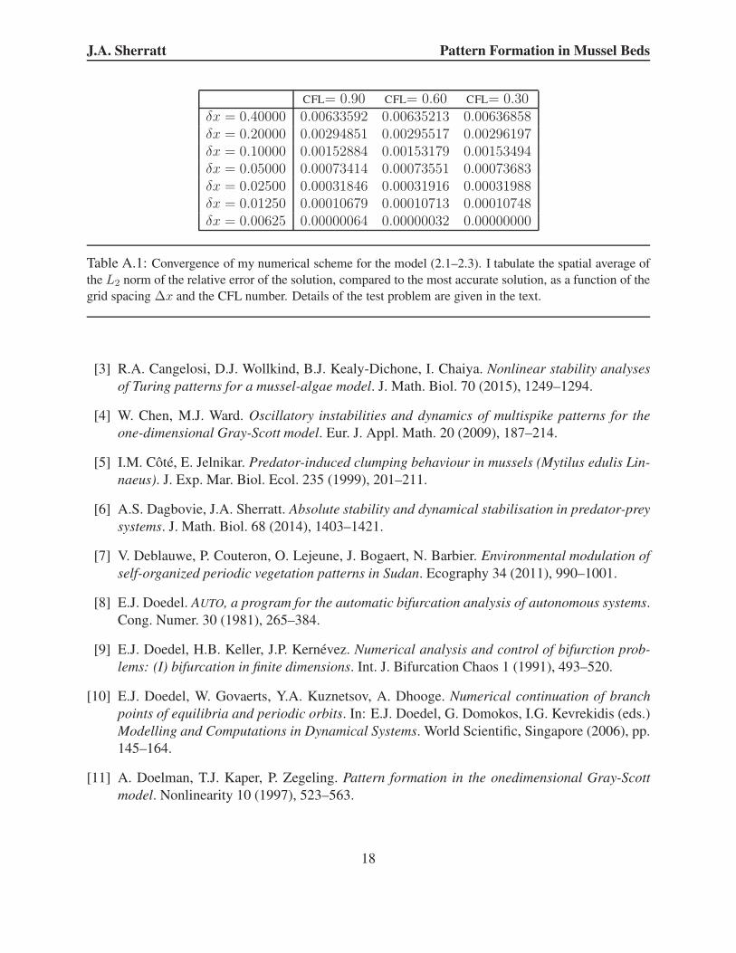
CFL= 0.90 CFL= 0.60 CFL= 0.30δx = 0.40000 0.00633592 0.00635213 0.00636858δx = 0.20000 0.00294851 0.00295517 0.00296197δx = 0.10000 0.00152884 0.00153179 0.00153494δx = 0.05000 0.00073414 0.00073551 0.00073683δx = 0.02500 0.00031846 0.00031916 0.00031988δx = 0.01250 0.00010679 0.00010713 0.00010748δx = 0.00625 0.00000064 0.00000032 0.00000000

Table A.1: Convergence of my numerical scheme for the model (2.1–2.3). I tabulate the spatial average of

the L2 norm of the relative error of the solution, compared to the most accurate solution, as a function of the

grid spacing ∆x and the CFL number. Details of the test problem are given in the text.

[3] R.A. Cangelosi, D.J. Wollkind, B.J. Kealy-Dichone, I. Chaiya. Nonlinear stability analyses

of Turing patterns for a mussel-algae model. J. Math. Biol. 70 (2015), 1249–1294.

[4] W. Chen, M.J. Ward. Oscillatory instabilities and dynamics of multispike patterns for the

one-dimensional Gray-Scott model. Eur. J. Appl. Math. 20 (2009), 187–214.

[5] I.M. Cote, E. Jelnikar. Predator-induced clumping behaviour in mussels (Mytilus edulis Lin-

naeus). J. Exp. Mar. Biol. Ecol. 235 (1999), 201–211.

[6] A.S. Dagbovie, J.A. Sherratt. Absolute stability and dynamical stabilisation in predator-prey

systems. J. Math. Biol. 68 (2014), 1403–1421.

[7] V. Deblauwe, P. Couteron, O. Lejeune, J. Bogaert, N. Barbier. Environmental modulation of

self-organized periodic vegetation patterns in Sudan. Ecography 34 (2011), 990–1001.

[8] E.J. Doedel. AUTO, a program for the automatic bifurcation analysis of autonomous systems.

Cong. Numer. 30 (1981), 265–384.

[9] E.J. Doedel, H.B. Keller, J.P. Kernevez. Numerical analysis and control of bifurction prob-

lems: (I) bifurcation in finite dimensions. Int. J. Bifurcation Chaos 1 (1991), 493–520.

[10] E.J. Doedel, W. Govaerts, Y.A. Kuznetsov, A. Dhooge. Numerical continuation of branch

points of equilibria and periodic orbits. In: E.J. Doedel, G. Domokos, I.G. Kevrekidis (eds.)

Modelling and Computations in Dynamical Systems. World Scientific, Singapore (2006), pp.

145–164.

[11] A. Doelman, T.J. Kaper, P. Zegeling. Pattern formation in the onedimensional Gray-Scott

model. Nonlinearity 10 (1997), 523–563.

18


[12] J.J. Donker, M. van der Vegt, P. Hoekstra. Erosion of an intertidal mussel bed by ice- and

wave-action. Cont. Shelf Res. 106 (2015), 60–69.

[13] M.B. Eppinga, M. Rietkerk, W. Borren, E.D. Lapshina, W. Bleuten, M.J. Wassen. Regular

surface patterning of peatlands: confronting theory with field data. Ecosystems 11 (2008),

520–536.

[14] M.B. Eppinga, M. Rietkerk, M.J. Wassen, P.C. De Ruiter. Linking habitat modification to

catastrophic shifts and vegetation patterns in bogs. Plant Ecol. 200 (2009), 53–68.

[15] B. Flemming, M. Delafontaine. Biodeposition in a juvenile mussel bed of the east Frisian

Wadden Sea (Southern North Sea). Aqua. Eco. 28 (1994), 289–297.

[16] J.C. Gascoigne, H.A. Beadman, C. Saurel, M.J. Kaiser. Density dependence, spatial scale

and patterning in sessile biota. Oecologia 145 (2005), 371–381.

[17] A. Ghazaryan, V. Manukian. Coherent structures in a population model for mussel-algae

interaction. SIAM J. Appl. Dyn. Syst. 14 (2015), 893–913.

[18] P. Gray, S.K. Scott. Autocatalytic reactions in the isothermal, continuous stirred tank reactor:

oscillations and instabilities in the system A+2B→3B; B→C. Chem. Eng. Sci. 39 (1984),

1087–1097.

[19] C.A. Klausmeier. Regular and irregular patterns in semiarid vegetation. Science 284 (1999),

1826–1828.

[20] O. Lejeune, M. Tlidi, P. Couteron. Localized vegetation patches: a self-organized response

to resource scarcity. Phys. Rev. E 66 (2002), 010901.

[21] S.A. Levin, R.T. Paine. Disturbance, patch formation, and community structure. Proc. Natl.

Acad. Sci. USA 71 (1974), 2744–2747.

[22] Q.-X. Liu, E.J. Weerman, P.M. Herman, H. Olff, J. van de Koppel. Alternative mechanisms

alter the emergent properties of self-organization in mussel beds. Proc. R. Soc. Lond. B 14

(2012), 20120157.

[23] Q.-X. Liu, A. Doelman, V. Rottschafer, M. de Jager, P.M. Herman, M. Rietkerk, J. van de

Koppel. Phase separation explains a new class of self-organized spatial patterns in ecological

systems. Proc. Natl. Acad. Sci. USA 110 (2013), 11905-11910.

[24] H. Malchow. Motional instabilities in predator-prey systems. J. Theor. Biol. 204 (2000), 639–

647.

[25] S.M. Merchant, W. Nagata. Instabilities and spatiotemporal patterns behind predator inva-

sions with nonlocal prey competition. Theor. Pop. Biol. 80 (2011), 289–297.

19


[26] R. Naddafi, K. Pettersson, P. Eklov. Predation and physical environment structure the density

and population size structure of zebra mussels. J. N. Am. Benthol. Soc. 29 (2010), 444–453.

[27] R.T. Paine, S.A. Levin. Intertidal landscapes: disturbance and the dynamics of pattern. Ecol.

Monogr. 51 (1981), 145–178.

[28] A.J. Perumpanani, J.A. Sherratt, P.K. Maini. Phase differences in reaction-diffusion-

advection systems and applications to morphogenesis. IMA J. Appl. Math. 55 (1995), 19–33.

[29] J.D.M. Rademacher, A. Scheel. Instabilities of wave trains and Turing patterns in large do-

mains. Int. J. Bifur. Chaos 17 (2007), 2679–2691.

[30] J.D.M. Rademacher, B. Sandstede, A. Scheel. Computing absolute and essential spectra us-

ing continuation. Physica D 229 (2007), 166–183.

[31] A.B. Rovinsky, M. Menzinger. Chemical instability induced by a differential flow. Phys. Rev.

Lett. 69 (1992), 1193–1196.

[32] B. Sandstede, Stability of travelling waves. In: B. Fiedler (ed.) Handbook of Dynamical

Systems II. North-Holland, Amsterdam (2002), pp. 983–1055.

[33] B. Sandstede, A. Scheel. Absolute and convective instabilities of waves on unbounded and

large bounded domains. Physica D 145 (2000), 233–277.

[34] J.A. Sherratt. Numerical continuation methods for studying periodic travelling wave (wave-

train) solutions of partial differential equations. Appl. Math. Computation 218 (2012), 4684–

4694.

[35] J.A. Sherratt. History-dependent patterns of whole ecosystems. Ecol. Complex. 14 (2013),

8–20.

[36] J.A. Sherratt. Numerical continuation of boundaries in parameter space between stable and

unstable periodic travelling wave (wavetrain) solutions of partial differential equations. Adv.

Comput. Math. 39 (2013), 175–192.

[37] J.A. Sherratt. Using wavelength and slope to infer the historical origin of semi-arid vegetation

bands. Proc. Natl. Acad. Sci. USA 112 (2015), 4202–4207.

[38] J.A. Sherratt, G.J. Lord. Nonlinear dynamics and pattern bifurcations in a model for vegeta-

tion stripes in semi-arid environments. Theor. Pop. Biol. 71 (2007), 1–11

[39] J.A. Sherratt, J.J. Mackenzie. How does tidal flow affect pattern formation in mussel beds? J.

Theor. Biol. 406 (2016), 83–92.

[40] J.A. Sherratt, M.J. Smith, J.D.M. Rademacher. Locating the transition from periodic oscilla-

tions to spatiotemporal chaos in the wake of invasion. Proc. Natl. Acad. Sci. USA 106 (2009),

10890–10895.

20


[41] J.A. Sherratt, A.S. Dagbovie, F.M. Hilker. A mathematical biologist’s guide to absolute and

convective instability. Bull. Math. Biol. 76 (2014), 1-26.

[42] E. Siero, A. Doelman, M.B. Eppinga, J.D.M. Rademacher, M. Rietkerk, K. Siteur. Striped

pattern selection by advective reaction-diffusion systems: Resilience of banded vegetation on

slopes. Chaos 25 (2015), 036411.

[43] K. Siteur, E. Siero, M.B. Eppinga, J. Rademacher, A. Doelman, M. Rietkerk. Beyond Turing:

the response of patterned ecosystems to environmental change. Ecol. Complex. 20 (2014),

81–96.

[44] M.J. Smith, J.A. Sherratt. Propagating fronts in the complex Ginzburg-Landau equation gen-

erate fixed-width bands of plane waves. Phys. Rev. E 80 (2009), 046209.

[45] M.J. Smith, J.D.M. Rademacher, J.A. Sherratt. Absolute stability of wavetrains can explain

spatiotemporal dynamics in reaction-diffusion systems of lambda-omega type. SIAM J. Appl.

Dyn. Systems 8 (2009), 1136–1159.

[46] A.C. Staver, S.A. Levin. Integrating theoretical climate and fire effects on savanna and forest

systems. Am. Nat. 180 (2012), 211–224.

[47] S.A. Suslov. Numerical aspects of searching convective/absolute instability transition. J.

Comp. Phys. 212 (2006), 188–217.

[48] J.C. Tam, R.A. Scrosati. Distribution of cryptic mussel species (Mytilus edulis and M. trossu-

lus) along wave exposure gradients on northwest Atlantic rocky shores. Mar. Biol. Res. 10

(2014), 51–60.

[49] J. van de Koppel, M. Rietkerk, N. Dankers, P.M. Herman. Scale-dependent feedback and

regular spatial patterns in young mussel beds. Am. Nat. 165 (2005), E66–77.

[50] S. van der Stelt, A. Doelman, G. Hek, J.D.M. Rademacher. Rise and fall of periodic patterns

for a generalized Klausmeier-Gray-Scott model. J. Nonlinear Sci. 23(2013), 39–95.

[51] B. van Leeuwen, D.C. Augustijn, B.K. van Wesenbeeck, S.J. Hulscher, M.B. de Vries. Mod-

eling the influence of a young mussel bed on fine sediment dynamics on an intertidal flat in

the Wadden Sea. Ecol. Eng. 36 (2010), 145–153.

[52] A.K. wa Kangeri, J.M. Jansen, B.R. Barkman, J.J. Donker, D.J. Joppe, N.M. Dankers. Per-

turbation induced changes in substrate use by the blue mussel, Mytilus edulis, in sedimentary

systems. J. Sea Res. 85 (2014), 233–240.

[53] R.H. Wang, Q.-X. Liu, G.Q. Sun, Z. Jin, J. van de Koppel. Nonlinear dynamic and pattern

bifurcations in a model for spatial patterns in young mussel beds. J. R. Soc. Interface 6

(2009), 705–718.

21


[54] E.J. Weerman, J. Van Belzen, M. Rietkerk, S. Temmerman, S. Kefi, P.W.J. Herman, J. van

de Koppel. Changes in diatom patch-size distribution and degradation in a spatially self-

organized intertidal mudflat ecosystem. Ecology 93 (2012), 608-618.

[55] J.T. Wootton. Local interactions predict large-scale pattern in empirically derived cellular

automata. Nature 413 (2001), 841–844.

[56] Y.R. Zelnik, E. Meron, G. Bel. Gradual regime shifts in fairy circles. Proc. Natl. Acad. Sci.

USA 112 (2015), 12327–12331.

22

Using Numerical Bifurcation Analysis to Study Pattern ... · J.A. Sherratt Pattern Formation in...

Documents

Transcript of Using Numerical Bifurcation Analysis to Study Pattern ... · J.A. Sherratt Pattern Formation in...