USING MARKOV DECISION MODELS AND RELATED TECHNIQUESFOR PURPOSES OTHER THAN SIMPLE OPTIMIZATION:

ANALYZING THE CONSEQUENCES OF POLICY ALTERNATIVESON THE MANAGEMENT OF SALMON RUNS

Roy MENDELSSOHNl

ABSTRACT

The mathematics of Markov decision processes and related techniques are used to analyze a modelrelevant to salmon management. It is shown that the choice ofgrid can have a significant effect on theresults obtained. Optimal policies that maximize total expected discounted return may be too variable.Smoothing costs are included to trade off long-run total return against the smoothness of the year-to­year fluctuations in the allowed harvest. Simpler, approximate policies that have a smoothing effectare also found. Preliminary analysis suggests the results are robust against misspecification of theparameters of the model. Concepts such as maximum sustainable yield would seem to impute a veryhigh smoothing cost and are probably not practical for fish populations with a significant degree ofrandomness.

The history of most managed natural populationsis one of sizable, nondeterministic variations inthe dynamics of the population. This observedvariation tends to have two sources: The firstsource is actual randomness in the system, such asthat due to environmental variability, which willexist no matter how accurate our models become;and the second source is the inaccurate or incom­plete speCification of the transition probabilitiesthemselves. Standard production models(Schaefer 1954; Pella and Tomlinson 1969; Fox1970,1971,1975) assume deterministic dynamics,as do most recent bioeconomic analyses, as inClark (1976) or Anderson (1977). For randomlyvarying populations, at best only extremely lowharvests may be sustainable year to year, and it isnot difficult to develop realistic scenarios wherepolicies that are sustainable in a deterministicmodel would cause possible depletion in a stochas­tic model.

In this paper, the latest tools from stochasticoptimization, particularly in the area of Markovdecision problems (MDP's) are used to analyze amodel relevant to salmon management. The view­point taken is that of the analyst, who mustanalyze trade offs and provide a decision makerwith as few policies as possible that contain the

lSouthwest Fisheries Center Honolulu Laboratory, NationalMarine Fisheries Service, NOAA, Honolulu, HI 96812.

Manuscript accepted September 1979.FISHER)' BULLETIN: VOL. 78, NO. I, 1980.

maximum amount of information, rather thanthat ofthe decision maker, who ultimately decidesif a particular concern or trade off is worthwhile.The salmon model is used as an example-the goalis to gain insight into managing randomly varyingpopulations.

Ricker (1958) appears to be the first to examinethe effects ofvariability on management. He usedintuition and simulation to arrive at policies thatare of the same general form as many of thepolicies to be discussed in this paper. However,Ricker presented no systematic way ofdevelopingoptimal policies and made the incorrect assump­tion that the long-run stochastic behavior willhave a mean equal to the deterministic equilib­rium yield, with noise around this mean.

Reed (1974) derived qualitative properties ofop­timal policies ifthe random variable has a mean of1, ifit affects the population dynamics in a multi­plicative manner, and if it has costs when thesystem is shut down (no harvesting) and thenstarted up again (resumption of harvesting).Reed's results are not relevant to the model dis­cussed in this paper, since he assumed the deter­ministic population model is concave, while themodels examined in what follows are pseudocon­cave. A more complete treatment of one dimen­sional stochastic growth models can be found inMendelssohn and Sobel (in press).

Walters (1975) and Walters and Hilborn (1976,1978) discussed a variety oftopics as the concerns

35

subject to O~Yt~t; and Equation (1.1)

maximizeE [~ aJ - 1 p(Xt -Yt)] (1.2b)t= 1

However, for many decision making situations,total expected discounted harvest may be a prefer­able criterion, since a discount factor can repre­sent a measure of risk or uncertainty about thesystem, over and above the variability due to therandom variable d. More formally, if ex is a dis­count factor O~ex<l, the problem is to:

F1SHERY BULLETIN: VOL. 78, NO.1

tributed random variable, with mean a and var­iance b.

For deterministic versions ofEquation (1.1), theprimary objective of management is MSY(maximum sustainable yield), which is equivalentto the largest per period growth of the determinis­tic model. The stochastic equivalent ofthis criteri­on is to maximize the average per period harvest,or gain optimality. Mathematically, letting E bethe expectation operator, this is

(1.2a)max lim [T1

E ~ (Xt - Yt)]T t-l'-+~

wherep is a weighting factor, which could be 1 orcould represent the average weight of the salmonharvested.

All the results in this paper are for expecteddiscounted return with ex = 0.97. For ex = 1, Equa­tion (1.2a) must be used, since Equation (1.2b) isinfinite for most policies. The choice of ex = 0.97 isarbitrary, though numerical runs for ex rangingfrom 0.95 to 1.00 produced no significant changesin the results. When actually implementing amodel, a careful choice of ex must be made, and thesensitivity ofthe results to changes in the value ofex should be tested. It should be mentioned that ex =

1 is just as much a discount factor as any othervalue and implies certain temporal preferencesand attitudes towards risk that may notadequately reflect the decision maker's prefer­ences.

The shortcomings of Equation (1.1a) or (1.1b)should also be noted, such as no account is taken ofocean harvesting of the salmon, particularly by aforeign nation. This just reinforces the idea thatthe purpose ofthis analysis is not optimization per

The models to be analyzed were developed byMathews (1967) to describe the spawner-recruitrelationships of sockeye salmon, Oncorhynchusnerka, populations in two rivers that run into Bris­tol Bay, Alaska. Oceanographic and other factorsaffect the number ofrecruits to a degree where therelationships can be modeled by the random equa­tions:

THE MODEL

Wood River:xt+ 1 = exp(d) (4.077Yt) exp( -0.800yt)

d=NCO,0.2098) (1.1a)

Branch River:xt +1 = exp(d) (4.554Yt) exp( -1.845Yt)

d=NCO,0.3352) (LIb)

)f this paper. Some of the techniques they dis­cussed, particularly the filtering techniques (Wal­ters and Hilborn 1978), are only appropriate ifthemodel has an additive error term. While a Rickerspawner-recruit curve can be transformed to anadditive model, many models do not have this fea­ture.

I am presenting what I feel is an improved wayto smooth out the fluctuations in the year-to-yearharvests as compared with the method suggestedin Walters (1975) and show that the Bayesian(adaptive) model discussed in Walters and Hilborn(1976) has an optimal policy with a very simpleform that can be readily calculated.

Moreover, a rigorous approach is taken to definethe model on a grid and the effects of the gridchoice. None of the papers cited deal with thisimportant question; new results are presentedwhich show that the most serious effect ofthe gridis on the estimates of the long-run (ergodic) prob­abilities of the population dynamics when follow­ing a given policy. Particularly the tail propertiesof the ergodic distribution, i.e., the long-run prob­ability of low harvest or low population sizes, aremisestimated. This is a new finding even in theMDP literature, and has numerical implications,particularly when calculating the trade off be­tween the mean harvest of a given policy and thelong-run probability of undesirable events whenfollowing that policy.

whereYt is the number ofspawners in period t,Xt+l

is the (random) number of recruits in period t+ 1,and d=N(a, b) denotes that d is a normally dis-

36

Defining the Model ona Discrete Grid

(InXi+1 -Ina)P(d~lnXi+1 -In a) = <P~ a

The discrete probability when the action is Yt isequal to the total probability of going to any statein the interval (Xi' Xi + l ).

Ifzero is included as a state, the procedure needsto be modified slightly. Suppose the probability ofgoing to Xl is known for each decision y. Then anarbitrary fraction ofthis probability is assigned asgoing to the zero state. In this paper, one-half ofthe probability in the interval (O,XI ) is assigned tothe zero state. The results have been found not tobe sensitive to the value of the fraction; this isbecause zero is an absorbing state. Either thereexists a policy that never reaches (0, Xl) and hencenever reaches zero, or else with probability one thepopulation goes to zero in finite time. Hence, it isthe size of (0, Xl) that most influences the results,not the fraction of this total that is assigned togoing to the absorbing state.

Adding an absorbing state is sensible if the ab­sorbing state is thought of as all states at lowenough population levels such that it would takeyears for the fishery to recover again, ifit recoversat all. Without the absorbing state, the models inEquation (l.la, b) will always recover in fairlyshort order. Since fisheries can be depleted, the

so that one method ofdefining the transition prob­abilities on a grid is:

rt-.(In Xi -a In a)P(d~ln Xi -In a) '¥

wherea = [R 1yt exp(-R2Yt )). Let <I> be the ~andardnormal integral for a random variable d = diu,and let Xi' Xi+ l be any two adjacent points on thegrid. Then:

(2.1)= P(d~lnw-Ina)

In order to make Equation (1.2) amenable tonumerical methods, it is necessary to define boththe state space and the action space on a discretegrid, and then to redefine the transition prob­abilities, etc., on this grid. Several authors (Fox1973; Bertsekas 1976; Hinderer 1978; Waldmann1978; Whitt 1978; Larraneta2) have suggestedtechniques to reduce MDP's to a grid and givebounds on the error due to the approximation. Ihave shown elsewhere (Mendelssohn3 ) that gridchoice can have a significant effect on the analysis.An optimal policy and the value of an optimalpolicy may not be greatly affected by the choice ofgrid, but the estimated probabilistic behavior ofthe population dynamics is affected significantlyhy the choice of grid.

A first effort then is to find an adequate grid forthe problem, a grid fine enough for both the de­sired accuracy and for realistic approximations ofobserved population sizes and coarse enough forcomputational efficiency. Increased computa­tional efficiency makes it reasonable to solvemany variations ofa given model, which allows fora more thorough exploration of the managementquestions of interest and their sensitivity to keyassumptions.

Several different grids were tried for Equation(1.2) for both the Branch and Wood Rivers.

To define Equation (1.2) on a given grid, supposea grid of k points has been chosen on which todiscretize the problem and assume, as is reason­able for this problem, that the reduced actionspace (how many spawners to leave) is equivalentto the state space (how many recruits are observedat the beginning of the period). From Equation(1.1), letting R I and R2 represent the parametersof the Ricker equation

MENDELSSOHN: USING MARKOV DECISION MODELS

se, but rather to provide the decision maker withadded insight and reasonable first choices.

'Larraneta, J. C. 1978. Approaches to approximate Mar­kov decision processes. Paper presented at Joint NationalORSAIl'lMS Meeting, Nov. 13·15, 1978, Los Ang., Calif.

"Mendelssohn, R. 1978. The effects of grid size and approx­imation techniques on the solutions of Markov decision prob·

lems. SWFC Admin. Rep. 20H, 15 p. Southwest Fish. Cent.Honolulu Lab., Nat!. Mar. Fish. Serv. NOAA, Honolulu, HI96812.

37

FISHERY BULLETIN: VOL. 78. NO.1

1.00

16,26,tU.90

>- .80

~iii .70

~ .60

~ .50

~ .40:0a .30

.20

./0

00 3

STATE I BRANCH RIVER}

1.0016,26

.90

.80

.70

.60

.50

.40

.50

.20

.10

00

FIGURE I.-Ergodic cumulative distributions for optimal har­vesting strategies on grid sizes of 16, 26, 51, and 101 points forthe Wood River and the Branch River.

3 4

STATE (WOOD RIVER)

finite time with probability one. However, for thelarger grids, there exist policies that are reducible,in the sense that if the chain does not start in theinterval (0, Xl)' it will never enter that interval.SinceP[xtE(O,xt )] = 0, and a fraction ofthis proba­bility has been assigned to the zero state, thenP(xt

=0) =O. When using the smaller grids that induceMarkov chains that are irreducible, the estimatedtime till absorption varies greatly also. For exam­ple, for the Branch River, ifP(xt = 0) = 0 andP(xt=w) = l/W-1), where w is a grid point and N isthe number of states, then a 16-point grid predictsabsorption with probability one after 2,000 itera­tions, the 26-point grid predicts only a 76% chanceof absorbtion after 2,000 iterations, and the 51­point grid predicts only a 17% chance of absorp­tion.

When maximizing total expected discounted re­turn, the discounted mean return depends on thevalues of these intermediate probability distribu­tions, so that coarser grids can be expected to un­derestimate the long-run value of the harvest.

Finally, for the Wood River, note that the 51­and 101-point grids have similar long-run be­havior. These results suggest that in order tofind

TABLE I.-Optimal policies for the different grid sizes.

inclusion ofan absorbing state would seem to be amore realistic assumption. It is included in whatfollows.

A coarser grid implies, in a sense, less informa­tion about the state of the system. As the interval(0, Xl) becomes large, our information has de­creased about the true state of the population andthis increased uncertainty is reflected in increasedrisk of absorbtion. Similarly, a finer grid impliesmore exact information-a grid should not be usedwhich is finer than the precision of the estimate ofthe population size.

Optimal policies for grids of 16,26,51, 101, and501 equally spaced points (including zero) for bothrivers are shown in Table 1. The optimal equilib­rium population for the equivalent deterministicmodels are shown also. All numbers are in units ofmillions of fish.

The optimal policies are all of the base stockvariety, i.e. it is optimal to harvest to a fixednumber ofspawners,or else not to harvest at all. Ifthe 50I-point grid is taken as the standard, it canbe seen that each coarser grid has as its base stocksize the grid point closest to the base stock size forthe 501-point grid.

Figure 1 gives the long-run (ergodic) cumula­tive distribution ofbeing in any state when follow­ing an optimal policy on grids of16, 26, 51, and 101points. Grid size can be seen to playa crucial partin estimating the probabilistic behavior of thepopulation. For the Wood River, extinction withprobability one is predicted on grids of 16 and 26points, while the p"robability is zero on grids of 51and 101 points, so long as zero is not the initialstate. Similar but not identical results are validfor the Branch River. It should be emphasized thatfor a = 1, Le., when the objective is given by Equa­tion (1.2a), the estimated average per period har­vest ofany policy depends entirely on the ergodicdistribution that arises from that policy. There­fore, this variation in estimated long-run behaviordue to changes in grid size is nontrivial.

Probability one of extinction occurs because fora finite state, irreducible Markov chain with anabsorbing state, the absorbing state is reached in

Wood River Grid size Branch River

YI ~ min (xl' 0.9333) 16 YI ~ m!n (XI' 0.3333)Yt ~ min (xt•0.840) 26 YI ~ min (xl' 0.4000)YI ~ min (xl' 0.700) 51 YI ~ min (XI' 0.3000)Yt ~ min (xt. 0.770) 101 YI ~ min (Xt. 0.3500)YI ~ min (xl' 0.742) 501 Yt ~ min (XI' 0.3500)

EquRibrium stock 0.735 Deterministic Equilibrium stock 0.345

38

The second method is to assume a general model ofthe form:

While these policies are similar in form topolicies that are optimal for a deterministic ver­sion of Equation (1.2), they differ greatly in theyear-to-year dynamics. There are two ways offinding the optimal deterministic policy. The firstway is to assume a general model of the form:

where as before,R1 andR2 are the parameters ofthe Ricker equation. The second method is prefer­able since it uses all the information available. Asd is a normal random variable with mean zero andvariance (1"2, it is easy to show that exp(d) is alognormal random variable with expectation exp(1f2 (1"2). Solving for the optimum sustained yield(OSY) population size for each river gives:

Branch River0.3450.63804

Wood River0.7351.11346

XOSy

OSY

MENDELSSOHN: USING MARKOV DECISION MODELS

good policies, it is only necessary to use a grid sizeof26 to 51 points for the problems under consider­ation. However, to analyze the long-run (prob­abilistic) behavior ofa given policy, it is necessaryto use a grid containing no fewer than 100 points.

It should be reemphasized that the reason forconsidering a coarser grid is that a smaller prob­lem size allows for many problems to be solved at asmall cost. This is desirable to obtain insight intothe sensitivity of the problem. However, it is pos­sible to solve quite large problems, making use ofavariety ofmethods to accelerate computations (seefor example Porteus 1971; Hastings and vanNunen 1977). For example, the 50I-point grid forthe Branch River used 1.80 s of CPU (central pro­cessing unit) time to perform the optimization.Computations, when smoothing costs are included(see Policy Analysis section), have 2,601 states.These used about 5 to 6 min of CPU time to per­form the computations, but at a cost of about $20.Our experience is that it is possible to obtainreasonable estimates using coarse grids and thatthis suffices for initial policy investigation. How­ever, it is worthwhile to reanalyze the final two orthree problems ofgreatest interest on a finer grid.

POLICY ANALYSIS

For the Wood River, the optimal policy for Equa­tion (1.2) is given by

Yt = minimum (o.no,xt)

and it produces a mean per period harvest of1.14758, and a standard deviation in the harvest of0.8963. The median harvest is 0.91, and no harvestOCcurs roughly 4.3% ofthe time. A harvest of25%or less of the mean harvest occurs roughly 15% ofthe time, while a harvest greater than the meanharvest occurs approximately 38% of the time.

Similarly, for the Branch River, an optimal pol­icy for Equation (1.2) is given by

Yt = minimum (0.300, Xt)

and it produces a mean per period harvest of0.6622, and a standard deviation in the harvest of0.6120. The median harvest is roughly 0.500;there is a 3.9% chance of no harvest. A harvest of25% of the mean harvest or less occurs roughly14.5% of the time, and a harvest greater than themean harvest occurs approximately 61% of thetime.

Both OSY values are lower than the mean perperiod harvests in the stochastic models, but thevariation is too high to allow this amount to beharvested each year. However, the XOSy level is agood estimate of the base stock size, and it isknown a priori from Mendelssohn and Sobel (inpress) that a base stock policy is optimal.

In the deterministic model, oncexOSY is reached,both the population size and the harvest size aremaintained at steady, equilibrium levels. An op­timal policy for the stochastic model, however,produces large fluctuations in both and may allowno harvesting 1 yr out of 25 in the long run. Formany fisheries, these "boom and bust" conditionsmay not be acceptable. Many people, especiallythose with interest or mortgage payments, as aremany fishermen, are concerned about smoothnessof income received as well as the total amountreceived. The final decision on the acceptableamount of fluctuation is, of course, up to the deci­sion maker with appropriate input.

There are several methods available to try tofind a balance between the smoothness of the ran­dom income stream and its total discounted ex­pected value. Walters (1975) and Walters and Hil­born (1978) suggested fixing a given mean harvest

39

FISHERY BULLETIN: VOL 78, NO.1

trade offbetween total income and the smoothnessof the received income stream.

For the Wood and Branch Rivers, two sets ofcomputations were performed. The first set as­sumes that y = e, i.e., there is an equal concern forincreases in allowable harvest as well as for de­creases. This is equivalent to e = 0.0 and c = y (orequivalently e). The motivation for this cost struc­ture is that fishermen typically resist any decreasein the allowed harvest, hence y>O. However, al­lowing increases in the harvest size often signalsfishermen to gear up and invest in equipment,thereby making it even more difficult to decreasethe allowable harvest later on. Therefore this costshould be equal to a cost due to a decrease in theharvest.

As a counterbalance to this, a second set of com­putations were performed with y>O but E = 0, i.e.,a cost only if the harvest is decreased. This isequivalent to c = e = y/2.

For the first set of computations, with e = 0.0and p = 1.0, values of c of 0.25, 0.50, 0.75, 1.00,1.25, 1.50, 1.75, and 2.00 were used. These areequivalent to relative values of ¥S, J4, %, !h, %, %,"Va, and 1. For the second set ofruns, with c = e, andp = 1.0, values of 0.25,0.50,0.75, 1.00 and 1.25were used. These are equivalent to a ratio of yIpequal to J4, !h, %, 1, 1J4. The results are sum­marized in Figure 2(a)-(m) and Figure 3(a)-(m),which show an optimal policy for each river foreach of these cases. All computations were per­formed on 26-point grids.

The figures are read as follows. Suppose Z washarvested last year and x is the observed popula­tion size this period. Find the point (x, z) on thegraph and follow the arrow in that zone to theappropriate boundary as indicated. Then read offthe Z value ofthis point; this is the optimal amountto harvest during this period.

For example, ifc = 0.50, e = 0.00, xt = 0.84, andthe harvest last period was 0.28, Figure 2(b) showsthat the optimal policy for the Wood River is toharvest 0.28 this period. Note that the dashed lineis the equivalent base stock harvest with nosmoothing costs.

While the policies in Figures 2 and 3 are optimalfor the given relative values ofp, e, and c. they arecomplex in nature and would be difficult for alayperson to understand. Practical managementoften implies determining simpler, good but sub­optimal policies that achieve the same objectives.These policies are often more desirable since they

Z = Zt •°

4Mendelssohn. R. 1976. Harvesting with smoothingcosts. SWFC Admin. Rep. 9H, 26 p. Southwest Fish. Cent.Honolulu Lab., Nat!. Mar. Fish. Serv., NOAA, Honolulu, HI96812.

u, and then finding a policy that minimizes

lim E T1 f (Zt - u)2. This methodology de-

T--* ~ t=1

pends on the values of u chosen. It also determinesthe policy that minimizes the approximate long­run variance for a given long-run mean harvest.This is not equivalent to reducing the size of theyear-to-year fluctuations.

A second method is to include "smoothing costs"into the one-period return. This approach has beenstudied analytically by Mendelssohn.4 Let y be thecost of a unit decrease in the harvest from year toyear, and let E be the cost of a unit increase in theharvest from year to year.

IfZ was harvested last year, then net revenuesthis year, for any harvestzt> are decreased by

where (a)+ denotes the positive part ofa. An alter­nate form is to let e = (y-e)/2 and c = (y+ e)/2. Thenthe one-period return is:

One advantage to the smoothing cost approachover other approaches is that p, e, and e can benormalized so as to be interpreted as relativeprices. That is, the normalized values p = 1, elp,and elp can be interpreted as the value of havingthe between period harvest "smoothed" by one unitrelative to the value of one unit of additional har­vest. Actual relative values are often difficult todetermine. But by parameterizing on e and c, it ispossible to present a decision maker not only arange ofpossible "optimal" policies and their con­sequences, but also some feeling for the relative

Amended to Equation (1.2), this would imply aone-period net benefit of

40

MENDELSSOHN: USING MARKOV DECISION MODELS

are easier to implement and easier to explain therationale to the public.

As an example of suboptimal, approximatepolicies, the following nine modified base stockpolicies were examined:

Wood River

1) Base stock policy, base stock size = 0.84.2) Policy ofbase stock size of0.56 till 2.52, then a

base stock size of 0.84.

3) Policy ofbase stock size of0.56 till 1.40, then abase stock size of 0.84.

4) Harvest 0 till 0.28, harvest 0.28 till 0.84, a basestock size of0.56 till 2.52, then a base stock sizeof 0.84.

Branch River

5) Base stock policy, base stock size of 0.40.6) Base stock size of 0.4 till 1.6, then a base stock

size of 0.6.

6.72

6.16

5.60

5.D4

4.48

3.92

Z3.36

2.80

2.24

1.68

1.12

.56

0

6.72

(a) C·O.25 E·O.O (e) C·O.75 E.O.O

m

6.16 (b) C· 0.50 E·O.O

5.60

5.D4

4.48

3.92

Z3.36

2.80

2.24

1.68

1./2

.56

00

x

(d) C·1.00 E·O.O

m

2.24 2.80 3.36 3.92 4.48 5.04 5.60 6.16 6.72

x

FIGURE 2(a-m).-Optirnal policy functions for the Wood River for variouB aBBUmptionB about the relative value ofsmoothing COBte. (Seetext for details).

41

7) Base stock size of0.2 till 0.6, then a base stocksize ofOA.

8) Base stock size of0.2 till 1.0, then a base stocksize of 004.

9) Base stock size of 0.2 till 004, base stock size of004 till 1.2, base stock size of 0.6 after that.

These nine approximate policies were devisedby examining the functions that define the threeregions in Figures 2 and 3. These approximate theboundaries ofthe three regions where the smooth-

FISHERY BULLETIN: VOL. 78, NO.1

ing costs are one-fourth to one-half the per unitvalue ofthe harvest. The mean per period harvest,variance, standard deviation, median per periodharvest, etc. for these nine policies are given inTable 2.

Policies 3 and 4 for the Wood River and 8 and 9for the Branch River demonstrate how these ap­proximate policies tend toward smoothingpolicies. For example, policy 4 has the same me­dian harvest as the optimal base stock harvest,almost never closes the fishery, significantly de-

o

oII

o

2.24 2.80 3.36 3.92 4.48 5.04 5.60 6.16 6.72

(9) C-1.75

(h) C-2.00 E-O.O

m

o

3.92 4.48 5.04 5.60 6.16 6.72

o

......

(e) C-1.25 E- 0.0

(f) C-1.50 E-O.O

6.72

6.16

5.60

5.04

4.48

3.92

Z 3.36

2.80

2.24

1.68

1.12

.56

6.72

6.16

5.60

5.04

4.48

3.92

Z 3.36

2.80

2.24

1.68

1.12

.56

00

x x

FIGURE 2.-Continued.

42

MENDELSSOHN: USING MARKOV DECISION MODELS

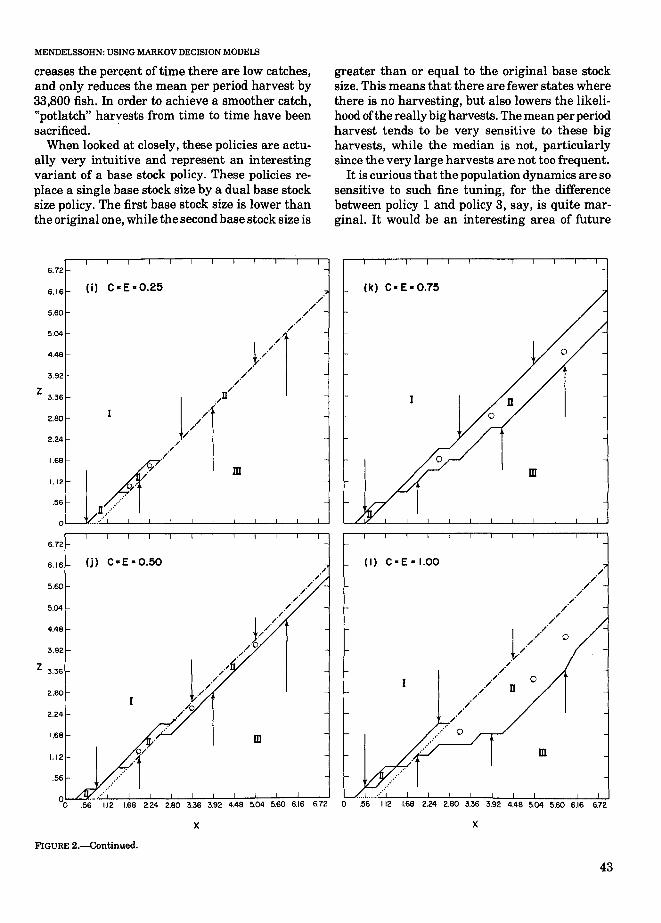
creases the percent of time there are low catches,and only reduces the mean per period harvest by33,800 fish. In order to achieve a smoother catch,"potlatch" harvests from time to time have beensacrificed. .

When looked at closely, these policies are actu­ally very intuitive and represent an interestingvariant of a base stock policy. These policies re­place a single base stock size by a dual base stocksize policy. The first base stock size is lower thanthe original one, while the second base stock size is

greater than or equal to the original base stocksize. This means that there are fewer states wherethere is no harvesting, but also lowers the likeli­hood ofthe really big harvests. The mean per periodharvest tends to be very sensitive to these bigharvests, while the median is not, particularlysince the very large harvests are not too frequent.

It is curious that the population dynamics are sosensitive to such fine tuning, for the differencebetween policy 1 and policy 3, say, is quite mar­ginal. It would be an interesting area of future

.56 1.12 1.68 2.24 2.80 3.36 3.92 4.48 5.04 5.60 6.16 6.72 0

(i) C·E-O.25

m

m

2.24 2.80 3.36 3.92 4.48 5.04 5.60 6.16 6.72

(k) C-E-0.75

(I) C - E - 1.00

m

m

///

vfj/f/

••••••'--••••.L._-"---'-_--'-----I_--'--_L.----'-_-"---'-_...L...J

(j) C' E • 0.50

6.72

6.16

5.60

5.04

4.48

3.92

Z3.36

2.80

2.24

1.68

1.12

.56

0

6.72

6.16

5.60

5.04

4.48

3.92

Z 3.36

2.80

2.24

1.68

1.12

.56

x x

FIGURE 2.-Continued.

43

FIGURE 2.-Continued.

research to determine guidelines for when finetuning would be expected to produce such "trim­ming" ofthe tails ofthe ergodic (long-run probabil­ity) distribution.

Including smoothing costs also tells us a greatdeal about traditional concepts of fisheries man­agement, such as MSY. It is clear from Figures 2and 3 that anything close to an MSY policy isoptimal only if the smoothing costs exceed the perunit value ofthe harvest. As whole systems oflawsfor regulating fisheries have been constructedaround the idea ofsmooth, constant harvests, it isclear that this imputes lower average catches, anda significant preference for constancy of the har­vest over total amount harvested.

The analysis has assumed that Equation (1.1) orsimilar equations are available, and that theparameter estimates are accurate (in this case,estimates of R1 , Rz ' and 0-2). In the latter case,management measures would seem more reason-

6.72

6.16

5.60

5.()q

4.48

3.92

Z 3.36

2.80

2.24

I.6S

1./2

.56

(m) C-E-1.25

m

2.24 2.S0 3.36 3.92 4.4S 5.04 5.60 6.16 6.72

x

FISHERY BULLETIN: VOL. 78, NO.1

able ifthey were known to be robust against mis­specifying the parameters. This involves knowinghow an optimal policy and total expected valuewould vary ifthe true underlying parameter val­ues differ from those specified, and also how theestimate of the long-run probability distributiondiffers from the true one.

Walters and Hilborn (1976) have examined asimilar question oftrying to solve the Bayes modelof this problem, Le., where there is an originalprior probability given to each value of theparameter, and this probability is updated eachperiod using Bayes theorem and the observed val­ues during the period. However, they could notobtain a solution, and Walters and Hilborn (1978)raised questions as to the validity of some of theirnumerical approximations.

Fortunately, qualitative results are possible forthis particular class of Bayes problems. Let e bethe parameter (or vector of parameters) underconsideration. Let Qo (e) be the initial prior dis­tribution on e, and let qn (e) be the updated priordistribution after n period has elapsed. Let 0 bethe set of all possible prior distributions. Then it isproven in van Hee (1977a) that if the state of thesystem is expanded to (xt> qt)' the resulting optimi­zation problem is Markovian. Following argu­ments similar to those in Scarf (1959) and van Ree(1977a) it follows that an optimal Bayes policytakes the form:

For each element q E 0, there is an x(q) suchthat:

do not harvest ifxt :;;;x(q)

harvest xt - x(q) ifxt>x(q).

For example, if(]'2 in the distribution ofd is itselfarandom variable, then each possible probabilitydistribution of 0-2 yields a possibly unique basestock size policy.

TABLE 2.-Vital statistics for the nine policies approximating the smoothing costpolicies for Wood and Branch Rivers.

Mean per Variance 01 % time % timeRelative value:period per period Standard % time less than greater than Median

River Policy harvest harvest deviation no catch 25% 01 mean mean catch catch smoothing/price

Wood 1 1.1357 0.8468 0.9202 5.6 16.8 39 0.98 0112 1.0993 0.5460 0.7389 1.7 10.7 39.8 0.98 1/8

3 1.1203 0.6506 0.8066 1.1 7.7 43.2 0.91 1/44 1.1019 0.5758 0.7588 0.02 10.47 40 0.98 1/2

Branch 5 0.6528 0.3982 0.6310 9.2 21.8 40 o.sOO 0116 0.6290' 02532 0.5032 9.1 21.5 37.2 0.500 1/47 0.6272 O.30n 0.5547 1.2 27.7 31.3 0.400 1/28 0.5920 0.2202 0.4693 1.9 35.7 26.3 0.500 3/89 0.5995 0.3038 0.5512 0.72 22.83 39.3 0.500 3/4

44

MENDELSSOHN: USING MARKOV DECISION MODELS

Van Hee (1977a) defined a set ofpolicies that heterms Bayes equivalent policies. For problemssuch as the salmon models under discussion, aBayes equivalent policy would be found as follows:

1) At the start ofthe period, the prior probabilitydistribution is q( 8).

2) The expected transition function (expectationwith respect to 8) is calculated, Le.,

p(d, q) =Jp(d I8)q(d8) (4.1)

where p( . I.) describes the dependence of the ran­dom variable don 8.

3)p(d, q) is used to solve a non-Bayesian Markovdecision process, with p(d, q) as the transitionfunction.

4)The optimal policy from step 3 above is usedfor one period.

5) q( 8) is updated using Bayes theorem and theobservations from the last period, and the updatedq( . ) is used in step 1 at the next time period.

It is worth noting that a Bayes eqivalent policy

4.S

z

4.4

4.0

3.6

3.2

2.8

2.4

2.0

1.6

1,2

.S

.4

(0) C·O.25 E·O.O (e) C·O.75 E·O.O

m

m

(d) C -1.00 E - 0.0

:1/(00' '.f- ,S 1.2 1.6 2,0 2.4 2,S3,2 3.6 4.0 4.4 4.S

4.8

4.4 (b) C-0.50 E-O.O

4.0

3.6

3.2

2.S

Z /

2.4

2.0

1.6

1.2 m

x x

FIGURE 3(a-m).-Optimal policy functions for the Branch River for various aBBumptions about the relative value of smoothing costs.(Sse text for details,)

45

FISHERY BULLETIN: VOL. 78. NO.1

is adaptive, as the prior distribution is updatedeach period. Moreover, it is not the same as fixinge at its estimated value, and using a fixed value ofe in step 3. The difference can be seen in theintegral in Equation (4.1). The reason for consider­ing Bayes equivalent policies is that van Hee(1977a, theorem 3.1) proved that for the modelsunder discussion, when the objective is given byEquation (1.2a) or (1.2b), then the Bayes equiva­lent policy is optimal for the full Bayes model. Forexample, in Walters and Hilborn (1976), the

parameter e is a scalar, i.e., Rz in our notation.Their problem, for which an optimal policy was notfound, can be solved by following a policy outlinedin the five steps above.

Many models will not have the necessary struc­ture for a Bayes equivalent policy to be optimal forthe full Bayes model, and unlike salmon manage­ment, estimates of the population size may not beavailable every year. A legitimate question is:suppose the present best estimate of e were to beused from hereafter. What would be the loss in

o

D

o

(g) C-1.75 E-O.O

4.8

4.4 (e) C- 1.25 E-O.O

4.0

3.6

3.2

2.8

Z2.4

2.0

1.6

1.2

.8m

.4

0

4.8

4.4

4.0

3.6

3.2

2.8

Z 2.4

2.0

1.6

(f) C -1.50 E -0.0

m

o D

o

(h) C-2.00 E-O.O

o

2.8 3.2 3.6 4.0 4.4 4.8

x xFiGURE 3.-Continued.

46

MENDELSSOHN: USING MARKOV DECISION MODELS

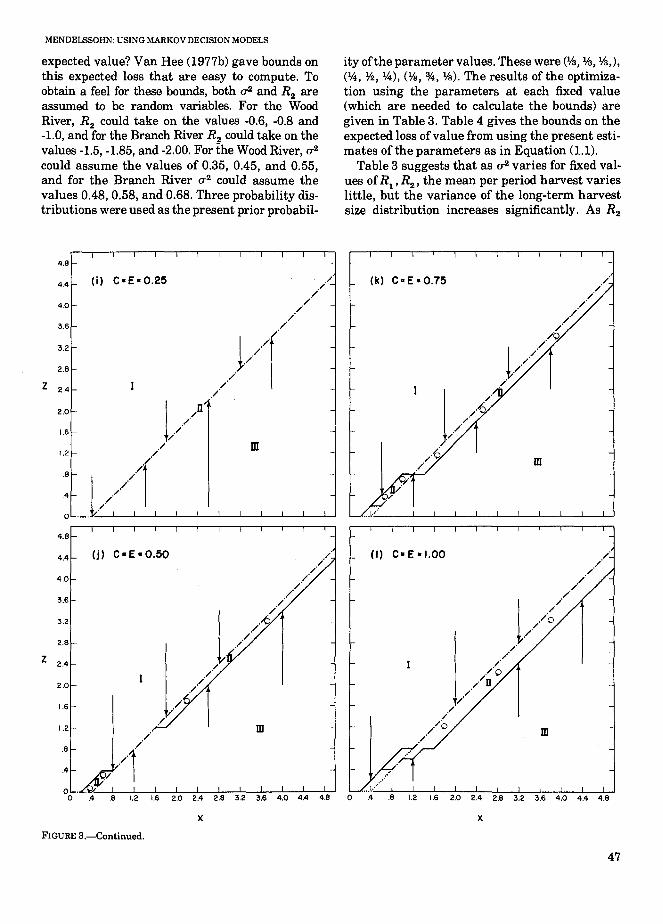
expected value? Van Hee (1977b) gave bounds onthis expected loss that are easy to compute. Toobtain a feel for these bounds, both u2 and R2 areassumed to be random variables. For the WoodRiver, R2 could take on the values -0.6, -0.8 and-1.0, and for the Branch River R2 could take on thevalues -1.5, -1.85, and -2.00. For the Wood River, u2could assume the values of 0.35, 0.45, and 0.55,and for the Branch River (]"2 could assume thevalues 0.48, 0.58, and 0.68. Three probability dis­tributions were used as the present prior probabil-

ity ofthe parameter values. These were (1f.I, 1f.I, 1f.I,),(14, %, 14), (!fe, %, !fe). The results of the optimiza­tion using the parameters at each fixed value(which are needed to calculate the bounds) aregiven in Table 3. Table 4 gives the bounds on theexpected loss ofvalue from using the present esti­mates of the parameters as in Equation (1.1).

Table 3 suggests that as u2 varies for fixed val­ues ofR1 ' R2 , the mean per period harvest varieslittle, but the variance of the long-term harvestsize distribution increases significantly. As R2

m

(k) C-E-O.75

m

4.4

4.0

3.6

3.2

2.8

Z 2.4

2.0

1.6

1.2

.8

.4

00

(j) C-E-O.50

m

.4 .8 1.2 1.6 2.0 2.4 2.8 3.2 3.6 4.0 4.4 4.8 2.4 2.8 3.2 3.6 4.0 4.4 4.8

xFIGURE 3.-Continued.

x

47

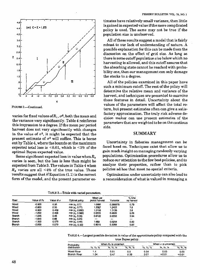
varies for fixed values ofR l , a 2 , both the mean andthe variance vary significantly. Table 4 reinforcesthis impression to a degree. Ifthe mean per periodharvest does not vary significantly with changesin the value of a 2 , it might be expected that thepresent estimate of a2 will suffice. This is borneout by Table 4, where the bounds on the maximumexpected total loss is <0.01, which is <1% of theoptimal Bayes expected value.

Some significant expected loss in value whenR2

varies is seen, but the loss is less than might beexpected from Table3. The values in Table 4 whenR2 varies are all <4% of the true value. Theseresults suggest that ifEquation (1.1) is the correctform of the model, and the present parameter es-

FIGURE 3.-Continued.

4.8

4.4

4.0

3.6

3.2

2.8

Z 2.4

2.0

1.6

(m) C- E-1.25

x

m

FISHERY BULLETIN: VOL. 78, NO. 1

timates have relatively small variance, then littleis gained in expected value ifthe more complicatedpolicy is used. The same may not be true if thepopulation size is unobserved.

All ofthese results suggest a model that is fairlyrobust to our lack of understanding of nature. Apossible explanation for this can be made from thediscussion on the effect of grid size. As long asthere is some cutoffpopulation size below which noharvesting is allowed, and this cutoff assures thatthe absorbing state cannot be reached with proba­bility one, then our management can only damagethe stocks to a degree.

All of the policies examined in this paper havesuch a minimum cutoff. The rest of the policy willdetermine the relative mean and variance of theharvest, and techniques are presented to examinethese features in detail. Uncertainty about thevalues of the parameters will affect the total re­turn, but present estimates often can give a satis­factory approximation. The truly risk adverse de­cision maker can use present estimates of theparameters that are weighted to be on the cautiousside.

SUMMARY

Uncertainty in fisheries management can befaced head on. Techniques exist that allow us togain much insight on managing randomly varyingpopulations. Optimization procedures allow us toreduce our attention to the few best policies, and toanalyze their properties, rather than to pickpolicies ad hoc that meet no special criteria.

Optimization under uncertainty can also lead toa reconsideration ofwhat is valued in managing a

TABLE 3.-Trials with varied parameters.

Mean per % timeRiver Value 01 R2 Value 01 <T Optimal policy period harvest Variance no harvest

Wood -0.800 0.35 mil (>ct, 0.7) 1.0680 0.390976 0.79Wood -0.600 0.55 min (xt, o.n) 1.2267 1.2422 7.8Wood -0.800 0.458 min (>ct, 0.980) 1.5108 1.3136 3.8Wood -1.000 0.458 min (xt, 0.560) 0.9225 0.4839 3.29Branch -1.845 0.48 min (xt, 0.35) 0,6122 0.2253 3.54Branch -1.845 0.68 mil (xt, 0.35)Branch -1.500 0.579 min (xt, 0.40) 1.989 0.5254 5.82Branch -2.000 0.579 min (xt, 0.30) 0.9075 0.3068 5.82

TABLE 4.-Largest poseible deviation in value of the approximate policy compared with thetrue Bayes policy.

Probability When R2 is uncertain When <T is uncertaindistribution V3, Y3f YJ 114,112,114 V8, 0/4, Ye 113, 113, 113 114,112,114 Va, 314, Va

Wood River 1.4 0.51 0.5 0.04 0.03 0.03Branch River 1.04 0.47 0.38 0.01 ..0,01 ..0.01

48

MENDELSSOHN: USING MARKOV DECISION MODELS

fishery-in the examples considered, some consis­tency in the amount harvested is a desirable al­ternative to high year-to-year fluctuations in theharvest size. But this reduced the average perperiod catch. Only in extreme situations, wherethe cost of smoothing out the catch is greater thanthe unit value of the catch, does any policy re­sembling MSY become optimal.

Finally, it is possible to obtain an understand­ing of how robust the management measures areto misspecifications of the underlying model. Thisis important, since the model is only a guide to ourdecision making, not the answer. In the modelsconsidered, the "best" policies are robust in view ofthis uncertainty.

A question not examined is the assumption thatthe population size is observed at the start of eachperiod. This too is usually costly, and inexact. Re­cently, I and E. J. Sondik developed an efficientalgorithm that addresses the relative merits ofdifferent sampling intervals for obtaining popula­tion estimates. 5 Together, all of these techniquesallow for an integrated, realistic approach to man­agement under uncertainty.

ACKNOWLEDGMENTS

Debra Chow provided invaluable assistance inprogramming the computer runs. DavidStoutemeyer of the University of Hawaii gavemuch useful advice on maximizing the efficiencyofthe optimization algorithm used. Lee Anderson,George Fishman, and Adi Ben-Israel gave impor­tant comments for improving an earlier version ofthis paper. The paper also benefited greatly fromthe comments of one of the referees and from C.Walters who tempered some remarks in a previousversion.

LITERATURE CITED

ANDERSON, L. G.1977. The economics of fisheries management. The

Johns Hopkins Univ. Press, Baltimore, 214 p.BERTSEKAS, D. P.

1976. Dynamic programming and stochastic con­trol. Acad. Press, N.Y., 396 p.

CLARK,C. W.1976. Mathematical bioeconomics: The optimal manage-

"Mendelssohn, R., and E. J. Sondik. 1979. The cost of in­formation seeking in the optimal management of random re­newable resources. SWFC Admin. Rep. H-79-12, 15p. Southwest Fish. Cent. Honolulu Lab., Natl. Mar. Fish. Serv.,NOAA, Honolulu, HI 96812.

ment of renewable resources. John Wiley and Sons,N.Y.,352p.

FOX,B. L.1973. Discretizing dynamic programs. J. Optim. Theory

Appl. 11:228-234.FOX, W. W.,JR.

1970. An exponential surplus-yield model for optimizingexploited fish populations. Trans. Am. Fish. Soc. 99:80­88.

1971. Random variability and parameter estimation forthe generalized production model. Fish. Bull., U.S.69:569-580.

1975. Fitting the generalized stock production model byleast-squares and equilibrium approximation. Fish.Bull., U.S. 73:23-37.

HASTINGS,N. A.J.,ANDJ.A. E. E. VANNUNEN.1977. The action elimination algorithm for Markov deci·

sian processes. In H. C. Tijms and J. Wessels (editors),Markov decision theory, p. 161·170. Proceedings of theAdvanced Seminar on Markov Decision Theory held atAmsterdam, the Netherlands, September 13-17, 1976.Mathematical Centre Tract 93. Mathematisch Centrum,Amsterdam.

HINDERER, K.1978. On approximate solution of finite-stage dynamic

program. Universitiit Karlsruhe, Fukultiit fiirMathematik, Bericht 8, 42 p.

MATHEWS, S. B.1967. The economic consequences of forecasting sockeye

salmon (Oncorhynchus nerka, Walbaum), runs to BristolBay, Alaska: Acomputer simulation study ofthe potentialbenefits to a salmon canning industry from accumte fore­casts of the runs. Ph.D. Thesis, Univ. Washington, Seat­tle, 225 p.

MENDELSSOHN, R., AND M. J. SOBEL.In press. Capital aceumulation and the optimization of

renewable resource models. J. Econ. Theory.PELLA, J. J., AND P. K. TOMLINSON.

1969. A genemlized stock production model. [In Engl.and Span.) Inter-Am. Trop. Tuna Camm., Bull. 13:419·496.

PORTEUS, E. L.1971. Some bounds for discounted sequential decision pro­

cesses. Manage. Sci. 18:7·11.REED, W.J.

1974. A stochastic model for the economic management ofa renewable animal resource. Math. BioscL 22:313-337.

RICKER, W. E.1958. Maximum sustained yields from fluctuating envi­

ronments and mixed stocks. J. Fish. Res. Board Can.15:991-1006.

SCARF,H.1959: Bayes solutions of the statistical inventory prob·

lem. Ann. Math. Stat. 30:490·508.SCHAEFER, M. B.

1954. Some aspects of the dynamics of populations impor­tant to the management of the commercial marinefisheries. Inter-Am. Trop. Tuna Comm., Bull. 1:25-56.

VAN HEE, K. M.1977a. Adaptive control of specially structured Markov

chains. In M. Schill (editor), Dynamische optimierung,p. 99-116. Bonner Mathematische Schriften 98, Bonn.

1977b. Approximations in Bayesian controlled Markovchains. In H. C. Tijms and J. Wessels (editors), Markov

49

decision theory, p. 171-182. Proceedings of the AdvancedSeminar on Markov Decision Theory held at Amsterdam,the Netherlands, September 13-17, 1976. MathematicalCentre Tract 93. Mathematisch Centrum, Amsterdam.

WALDMANN, K.-H.1978. On approximation of dynamic programs. Preprint

No. 439, Fachberech Mathematik, TechnischeHochschule Darmstadt, 17 p.

WALTERS, C. J.1975. Optimal harvest strategies for salmon in relation to

50

F1SHERY BULLETIN; VOL. 78, NO.1

environmental variability and uncertain productionparameters. J. Fish. Res. Board Can. 32:1777-1784.

WALTERS, C. J., AND R. HILBORN.1976. Adaptive control of fishing systems. J. Fish. Res.

Board. Can. 33:145-159.1978. Ecological optimization and adaptive manage­

ment. Annu. Rev. EcoJ. Byst. 9:157-188.WHITT, W.

1978. Approximations of dynamic programs, 1. Math.Oper. Res. 3:231-243.