Using Markov Chains to Analyze GAFOs

Kenneth A. De JongComputer Science Department

George Mason UniversityFairfax, VA 22030

E-mail: kdejong@gmu.edu

William M. SpearsDiana F. Gordon

Navy Center for Applied Research in Artificial IntelligenceCode 5510

Naval Research LaboratoryWashington, D.C. 20375-5320

E-mail: spears,gordon@aic.nrl.navy.mil

Abstract

Our theoretical understanding of the properties of genetic algorithms(GAs) being used for function optimization (GAFOs) is not as strongas we would like. Traditional schema analysis provides some first orderinsights, but doesn’t capture the non-linear dynamics of the GA searchprocess very well. Markov chain theory has been used primarily forsteady state analysis of GAs. In this paper we explore the use oftransient Markov chain analysis to model and understand the behaviorof finite population GAFOs observed while in transition to steadystates. This approach appears to provide new insights into thecircumstances under which GAFOs will (will not) perform well. Somepreliminary results are presented and an initial evaluation of the meritsof this approach is provided.

1 INTRODUCTION

At the previous FOGA workshop the claim was made that our theoretical understandingof the properties of genetic algorithms (GAs) being used for function optimization (i.e.,GAFOs) was quite weak (De Jong, 1992). Traditional schema analysis provides insightinto the optimal allocation of trials when maximizing cumulative profits is the goal(Holland, 1975), but doesn’t say much about global function optimization. Staticanalysis of functions regarding their ‘‘deceptiveness’’ provides some insights into whatkinds of functions are difficult to optimize with a GA (Goldberg, 1987), but is a ‘‘firstorder’’ theory in the sense that it doesn’t include the effects of the non-linear dynamicsof the GA search process. Traditional Markov chain analysis provides insight into thelong term, steady state behavior of large population GAs (Davis and Principe, 1991; Nixand Vose, 1992; Vose, 1992; Suzuki, 1993; Rudolph, 1994), but says little about thetransient observable behavior of implementable GAFOs. Markov chains have also beenused to model specific features of GAs, such as selection, genetic drift, niching, etc. (DeJong, 1975; Goldberg and Segrest, 1987; Mafoud, 1993; Horn, 1993).

We feel that recent theoretical developments along with advances in computationalpower have set the stage for a more complete analysis of GAFOs via Markov chains. Inthis paper we present our ideas as to how previous Markov chain analyses can beextended to provide a stronger GAFO theory capable of explaining and predicting thebehavior of GAFOs on various classes of optimization problems. We feel that such atheory must simultaneously take into account the characteristics of the particular GAFObeing used (generational, elitist, etc.), the internal search space representation (binary,gray code, etc.), the operators used (form and rate of crossover, etc.), the non-lineardynamics of the search process, and the characteristics of the function to be optimized.

As a consequence, we are uncomfortable with the notion of a ‘‘GA-hard problem’’independent of these other details, unless we mean by such a phrase that no choice ofGA properties, representations, and operators exist that make such a problem easy for aGAFO to solve. There are such problems, of course. Needle-in-a-haystack problems arethe canonical example, but are equally difficult for any other optimization algorithm.

As soon as we leave this class of hard search problems, we find ourselves in situations inwhich the difficulty of finding the optimum is a function of both the particular GAFObeing used as well as the optimization problem. Changes to either can increase ordecrease the observed difficulty. Said another way, the difficulty of a particular GAFOsituation is strongly correlated to how well matched the features of a particular GAFOare to the characteristics of a given problem. High degrees of consonance correspond toour informal notion of a GA-easy situation, and significant dissonance results in GA-hard situations. As GAFO engineers we can and do frequently increase the consonanceof a particular situation by changing representations, operators, etc.

From this perspective a GAFO theory should provide ways of measuring degrees ofhardness of a particular situation. It should provide insight into the effects that changesin representation, operators, etc. have on hardness, and for a given GAFO makepredictions about the kinds of problems with which it will have difficulties. We presentthe initial steps toward such a theory in the remaining sections.

2 MEASURING GA PERFORMANCE AND HARDNESS

The standard measures of performance for optimization algorithms involve convergenceproperties (i.e., the ability to find an optimum) as well as convergence rates (how quicklythey are found). Since GAFOs are parallel, population-based stochastic searchprocedures, there are a number of possible definitions of convergence. The simplestnotion is that ultimately a GAFO population converges to a uniform populationconsisting of n copies of a single individual which may or may not correspond to aglobal optimum.

Since most GAFOs are run with non-zero mutation rates, this simple form ofconvergence seldom occurs, unless one "anneals" the mutation rate over time. Withoutan annealing mechanism GAFOs settle into a dynamic equilibrium in which theexploratory pressures of mutation and crossover are balanced by the exploitativepressure of selection. Moreover, since mutation is active, every point in the space hassome non-zero probability of being visited. Hence, it is trivial to show that a globaloptimum will be visited infinitely often when a GAFO is left to run in this state ofdynamic equilibrium.

As a consequence, most GAFO practitioners measure performance in terms of theaverage (or best) points in the current population, or in terms of monotonically non-decreasing ‘‘best so far’’ curves which plot, as a function of the number of samples (orgenerations), the best point found so far in the search process regardless of whether ornot that point is currently represented in the population.

Some natural questions related to such performance measures immediately arise. Howlikely is it that, if I look at the contents of the kth generation, it will contain a copy of theoptimum? What is the expected waiting time until a global optimum is encountered forthe first time? How long must we wait before a point is encountered that is within someerror tolerance of the optimum? How much variance is there in such measures from runto run? How much are such measures affected by changes in population size, mutationrates, etc.?

As GA practitioners we constantly look for ways to improve the performance of ourGAFOs with respect to these measures. Situations which exhibit shorter mean waitingtimes and smaller variances correspond to our notion of GA-easy situations, andsituations with longer mean waiting times and higher variances are viewed as harder.Consequently, these statistics appear to be natural quantitative measures of the difficultyof a particular GAFO situation.

3 MARKOV MODELS OF SIMPLE GAs

If we are to use such statistics as the mean and variance of waiting times as measures ofhardness, random process theory would seem to provide an appropriate set of tools fordescribing the behavior of stochastic GAFOs. Historically, it has been quite natural tomodel simple GAs as Markov processes in which the ‘‘state’’ of the GA is given by thecontents of the current population (De Jong, 1975; Goldberg & Segrest, 1987). One canthen imagine a state space of all possible populations and study the characteristics of thepopulation trajectories (the Markov chains) a GA produces from randomly generatedinitial populations.

Most of the analytic results obtained from this approach are derived using infinitepopulation models and involve characterizing steady state behavior (Davis and Principe,1991; Vose, 1992; Suzuki, 1993; Rudolph, 1994). It is considerably more difficult to getanalytic results concerning means and variances of waiting times for Markov models offinite population GAFOs. However, increases in computer technology now permit thevisualization and computational exploration of such models as the first steps indeveloping such a theory. We explore such an approach in this paper.†

Among the many papers on Markov models of GAs, the Nix and Vose model (1992) isparticularly well suited to serve as the basis for our GAFO theory. We begin with a briefsummary of their model and notation.

3.1 Summary of the Nix and Vose Markov Model

The Nix and Vose Markov model is intended to represent a simple generational GAconsisting of a finite population, a standard binary integer representation, standardmutation and crossover operators, and fitness-proportional selection. Fitness scaling,elitism, and other GAFO-oriented features are not modeled.

If l is the length of the binary strings, then r = 2l is the total number of possible strings.If n is the population size, then the number of possible populations, N, corresponding tothe number of possible states is:

N =

��

r − 1n + r − 1�� (1)

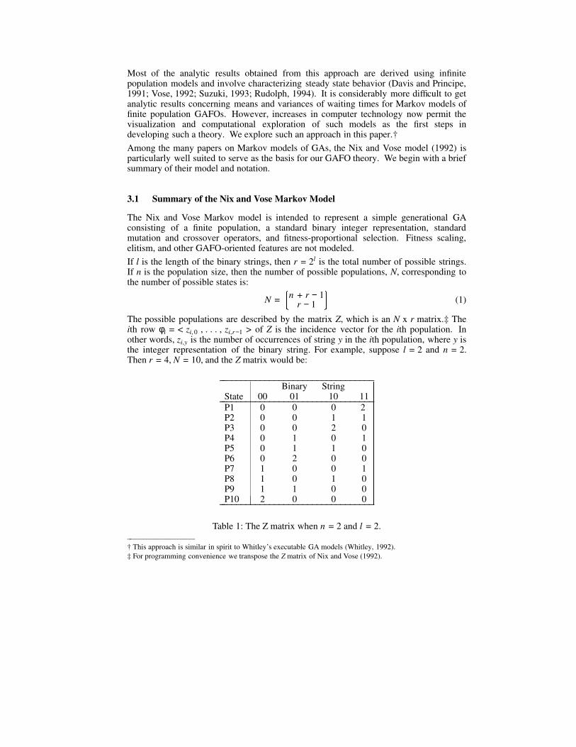
The possible populations are described by the matrix Z, which is an N x r matrix.‡ Theith row φi = < zi, 0 , . . . , zi,r−1 > of Z is the incidence vector for the ith population. Inother words, zi,y is the number of occurrences of string y in the ith population, where y isthe integer representation of the binary string. For example, suppose l = 2 and n = 2.Then r = 4, N = 10, and the Z matrix would be:

_________________________________Binary String

State 00 01 10 11_________________________________P1 0 0 0 2P2 0 0 1 1P3 0 0 2 0P4 0 1 0 1P5 0 1 1 0P6 0 2 0 0P7 1 0 0 1P8 1 0 1 0P9 1 1 0 0P10 2 0 0 0_________________________________��������������

��������������

��������������

Table 1: The Z matrix when n = 2 and l = 2.__________________

† This approach is similar in spirit to Whitley’s executable GA models (Whitley, 1992).

‡ For programming convenience we transpose the Z matrix of Nix and Vose (1992).

Nix and Vose then define two mathematical operators, F and M, where F is determinedfrom the fitness function, and M depends on the mutation rate µ, crossover rate χ, andform of crossover and mutation used.†

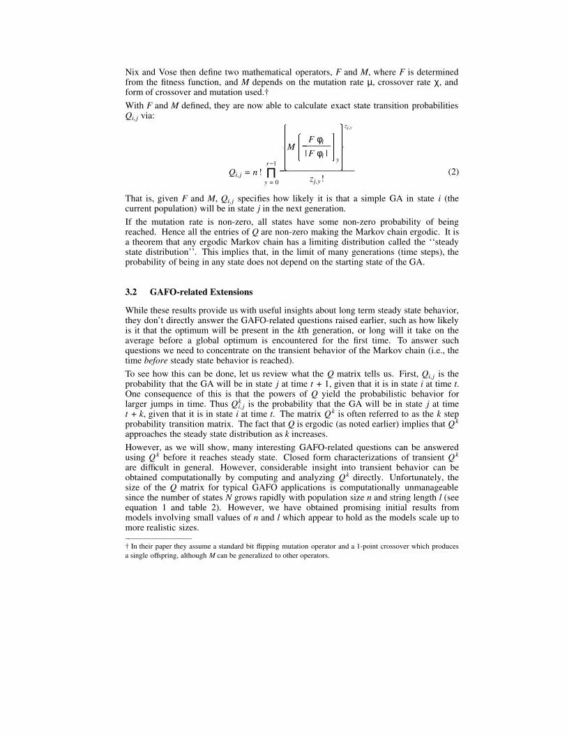
With F and M defined, they are now able to calculate exact state transition probabilitiesQi, j via:

Qi, j = n ! y = 0Πr−1

zj,y!

�����M

���| F φi |

F φi_______

�

y

���

zj,y

_________________(2)

That is, given F and M, Qi, j specifies how likely it is that a simple GA in state i (thecurrent population) will be in state j in the next generation.

If the mutation rate is non-zero, all states have some non-zero probability of beingreached. Hence all the entries of Q are non-zero making the Markov chain ergodic. It isa theorem that any ergodic Markov chain has a limiting distribution called the ‘‘steadystate distribution’’. This implies that, in the limit of many generations (time steps), theprobability of being in any state does not depend on the starting state of the GA.

3.2 GAFO-related Extensions

While these results provide us with useful insights about long term steady state behavior,they don’t directly answer the GAFO-related questions raised earlier, such as how likelyis it that the optimum will be present in the kth generation, or long will it take on theaverage before a global optimum is encountered for the first time. To answer suchquestions we need to concentrate on the transient behavior of the Markov chain (i.e., thetime before steady state behavior is reached).

To see how this can be done, let us review what the Q matrix tells us. First, Qi, j is theprobability that the GA will be in state j at time t + 1, given that it is in state i at time t.One consequence of this is that the powers of Q yield the probabilistic behavior forlarger jumps in time. Thus Qi, j

k is the probability that the GA will be in state j at timet + k, given that it is in state i at time t. The matrix Qk is often referred to as the k stepprobability transition matrix. The fact that Q is ergodic (as noted earlier) implies that Q k

approaches the steady state distribution as k increases.

However, as we will show, many interesting GAFO-related questions can be answeredusing Q k before it reaches steady state. Closed form characterizations of transient Q k

are difficult in general. However, considerable insight into transient behavior can beobtained computationally by computing and analyzing Qk directly. Unfortunately, thesize of the Q matrix for typical GAFO applications is computationally unmanageablesince the number of states N grows rapidly with population size n and string length l (seeequation 1 and table 2). However, we have obtained promising initial results frommodels involving small values of n and l which appear to hold as the models scale up tomore realistic sizes.__________________

† In their paper they assume a standard bit flipping mutation operator and a 1-point crossover which produces

a single offspring, although M can be generalized to other operators.

_____________________________________________________________String length l

Popsize n 1 2 3 4 5_____________________________________________________________1 2 4 8 16 322 3 10 36 136 5283 4 20 120 816 5,9844 5 35 330 3,876 52,3605 6 56 792 15,504 376,9926 7 84 1,716 54,264 2,324,7847 8 120 3,432 170,544 12,620,2568 9 165 6,435 490,314 61,523,7489 10 220 11,440 1,307,504 273,438,88010 11 286 19,448 3,268,760 1,121,099,408_____________________________________________________________��������������

��������������

��������������

Table 2: The value of N as a function of l and n.

4 Visualizing Markov Models

Before we develop our GAFO theory in more detail, we take a slight diversion toindicate a side benefit to having Qk directly available, namely to allow for visualizationof the changing probability distributions Qk represents. We have been pleasantlysurprised at the insight even simple visualization techniques provide concerning theeffects that various GA and fitness function features have on Q k. † We illustrate thisbriefly with an example involving visualizing Qk as an image, where the gray level ofcoordinate (i,j) reflects the probability that the GA will move from state i to state j in ksteps. White indicates high probability, while black indicates low probability.

Figures 1-4 illustrate this for various Qk in which n = 3 and l = 3. To highlight theeffects of genetic operators, Figures 1 and 2 show Q k with a flat fitness function (i.e., noselection pressure). Figure 1 shows Q k when only mutation is active (µ = 0.01 andχ = 0.0). The left most image, representing Q1 , has two interesting features. A brightdiagonal line is clearly visible, indicating that significant changes in the population inone generation are very unlikely. Also, notice the interesting fractal-like patternsexhibited. This appears to be an artifact of the particular lexicographic ordering of states(given by Nix and Vose, 1992). We are currently exploring other potentially morenatural orderings.

As one scans the images from left to right, notice that the changes in the probabilitydistribution are already evident in Q4 and quite striking in Q10 . The emerging verticallines represent the particular populations at which the steady state distribution willaccumulate most of its probability mass, i.e., those populations most likely to beobserved when the GA settles into its dynamic equilibrium.

Figure 2 shows the change in Qk when crossover is activated (µ = 0.01 and χ = 1.0). Itis interesting to compare Q1 in Figure 1 with Q1 in figure 2. The visual effect of turningon crossover is to make Q1 more diffuse, matching our intuition that crossover can makelarger changes more easily.__________________

† For additional evidence of the usefulness of visualizing Q, see Horn, Goldberg & Deb (1994).

Q1 Q4 Q10

Figure 1: Q k with no selection, µ = 0.01 and χ = 0.0.

Q1 Q4 Q10

Figure 2: Q k with no selection, µ = 0.01 and χ = 1.0.

Figure 3 illustrates the added effects of selection pressure on Q k by replacing the flatfitness function with f (y) = integer (y) + 1, where integer (y) returns the integerequivalent of the bit string y. Notice the visual confirmation of our intuition thatselection has an increasing effect on the probability distributions as the number ofgenerations (k) increases.

Finally, figure 4 illustrates the effects of increasing the mutation rate from µ = 0.01 toµ = 0.1. Notice that the vertical lines in Q10 form a different and much sharper patternthan they did in figure 3. This reflects the fact that increasing µ not only changes thesteady state probability distribution, but also decreases the number of generationsrequired to achieve a steady state distribution. Note that this does not imply that the

Q1 Q4 Q10

Figure 3: Qk with selection, µ = 0.01, and χ = 1.0.

Q1 Q4 Q10

Figure 4: Qk with selection, µ = 0.1, and χ = 1.0.

number of generations required to find the optimum has also decreased. This is easilyseen by observing that in the limit of µ = 0.5 the steady state distribution is reachedimmediately in generation 1 (i.e., Q = Qk for all k). In this extreme case the steady stateprobabilities are precisely the a priori probabilities given in equation 3 in the nextsection, since µ = 0.5 is equivalent to randomly initializing a population.

5 GAFO THEORY

We now show how Q k can be used to characterize the transient behavior of GAs. This inturn allows us to answer many questions related to the observable behavior of finitepopulation GAFOs. For the sake of clarity we will develop these results in two steps.

First, in this section, we will use Qk to give probabilistic answers to questionsconcerning the expected behavior of a GA at a particular point in time (i.e., during aparticular generation), and illustrate how that can provide considerable insight intoissues such as GA hardness.

Then, in section 6, we will extend these ideas to describe cumulative GA behaviorextending over multiple generations, which provides exact answers to GAFO-relatedquestions such as the expected waiting time until an optimum is first encountered.

5.1 Expected Behavior during the kth Generation

In this section we develop the theory which will allow us to answer questions such as:

1) What is the probability that the GA population will contain a copy of the optimumat generation k?

2) What is the probability that the GA population will have average fitness greaterthan some value at generation k?

3) What is the probability that the GA population will have diversity less than somevalue at generation k?

4) What is the expected best individual at generation k?

To answer such questions, we need only combine Q k with a set of initial conditionsconcerning a GA at generation 0. For this paper we make the reasonable assumption thatGA populations are randomly initialized. Thus, the a priori probability of the GA beingin state i at time 0, denoted as P(i @ 0), is:

P(i @ 0) = zi, 0! . . . zi,r−1!

n !____________

��r

1__

���

n

(3)

Since there are r = 2l possible strings, each string has a probability of r−1 of occurring,there are n strings in the population, and the multinomial distribution takes into accountthe different ways the strings can be inserted into the population to create a unique state.

Given this, we can now compute the probability that the GA will be in a particular state jat time k:

P(j @ k) = iΣ P(i @ 0) Qi, j

k (4)

by simply considering the probability of each possible k step transition, appropriatelyweighted by the a priori probabilities.

We can also compute probabilities over a set of states. Define a predicate PredJ and theset J of states that make PredJ true. Then the probability that the GA will be in one of thestates of J at time k is:

P(J @ k) = j∈ JΣ P(j @ k) (5)

It is also straightforward to compute related conditional probabilities such as theprobability that the GA is in one of the states of J at time t + k, given that it is in state iat time t:

P(J @ t +k | i @ t) = j∈ JΣ Qi, j

k (6)

This is easily generalized to give the probability that the GA will transition from one setof states to another. Let PredI be another predicate over the states, and denote I to be theset of states that make PredI true. Then the probability that the GA will be in one of thestates of J at time t + k, given that it is in one of the states of I at time t, is:

P(J @ t +k | I @ t) = P(I @ t)

i∈ IΣ��P(i @ t) P(J @ t +k | i @ t)

��

_____________________________(7)

which involves a renormalization over the states indexed by I. Note that equation 7simplifies to equation 6 when I is composed of one state, and is similar to equation 4when I is composed of all the states.

The nice feature of this formalization is that any predicate over the states (populations)can be used. Thus, if we are interested in optimality, we can define the set of states thatcontain at least one copy of an optimum, and compute the probability that the GA willactually be in one of these states at generation k. We can also define predicates thatselect states based on average fitness, fitness variance, diversity, and so on.

In fact we can generalize further to arbitrary functions f over the states and compute, forexample, the expected value of that function, at time k:

E[fk] = jΣP(j @ k) f(j) (8)

This allows us to compute for the kth generation the expected best fitness value, theexpected average fitness, expected diversity, or any other measure of interest that isdefined over the states.

We conclude this section by illustrating how these results can be used to answer the fourquestions posed at the beginning of this section:

1) To compute the probability that a GA will have in the population at time k at leastone copy of the optimum, use equation 5 with J as the set of all populationscontaining at least one copy of the optimum.

2) To compute the probability that a GA will have at time k a population with anaverage fitness greater than X, use equation 5 with J as the set of all populationshaving average fitness greater than X.

3) To compute the probability that a GA will have at time k a population withdiversity less than X, use equation 5 with J as the set of all populations havingdiversity less than X.

4) To compute the expected best fitness value in the population at time k, useequation 8 with f defined to return the maximum fitness in a given population.

5.2 Transient Behavior of GAs

These results can be used directly to provide insight into the effects that fitness functions,choice of operators, etc. have on the transient behavior of GAs. For example, tounderstand GAFO behavior better we might consider plotting the probability that a GAwill have a copy of the optimum in its population at generation k for k = 1,...,K usingequation 5 above.

Figure 5 illustrates this for the simple case of l = 2, n = 5 and the fitness functionf (y) = integer (y) + 1. Using random search as a baseline, we show how the probabilityof having a copy of the optimum in the population at generation k changes dynamicallyover time, and how these probability curves are affected by turning crossover off(χ = 0.0) and on (χ = 1.0) while holding the mutation rate fixed at µ = 0.1.

2 5 10 20 50

0.7

0.8

0.9

1

SuccessProb

Generations (log scale)

•

••

•• • • • • • • • • • • • • • •• ••••••••••••••••••••••••••••••••••••••••••••••••••• ••••••••••••••••••••••••••••

crossover

no crossover

random search

Figure 5: GA behavior on f (y) = integer (y) + 1

The probability curve for random search is included for comparative purposes. Since weare focusing on generation-oriented questions, we conceptualize random search as a GAwhich produces n random strings each generation. If there is a unique optimum amongthe r = 2l strings, then the probability that this random process will contain at least onecopy of the optimum string in generation k is constant and given by:

1 −

���r

r − 1_____

���

n

There are several interesting observations one can draw from the probability curves infigure 5. First, note that these are not cumulative probabilities indicating whether or notthe optimum has been encountered at least once by generation k. Rather, they predictthe likelihood of generation k containing a copy of the optimum regardless of whether ornot the optimum appeared in an earlier generation. These curves confirm our intuitionthat GAs settle into a dynamic steady state in which there are no changes in theprobability of producing an optimal string.

They also confirm our notion that there are situations in which crossover clearlyimproves the likelihood of generating optimal strings, and that even without crossover a

GA with moderate mutation rates is more likely to do so than random search.

These probability curves can also be used to study the effect that different classes offitness functions have on the ‘‘hardness’’ of the situation. To illustrate this, we simplypermute the fitness values assigned to the r = 2l strings by the original fitness function.In the previous example f assigned the values {1,2,3,4} to the strings {00,01,10,11}respectively. Permuting the 4 fitness values produces 4! = 24 distinct fitness functions.

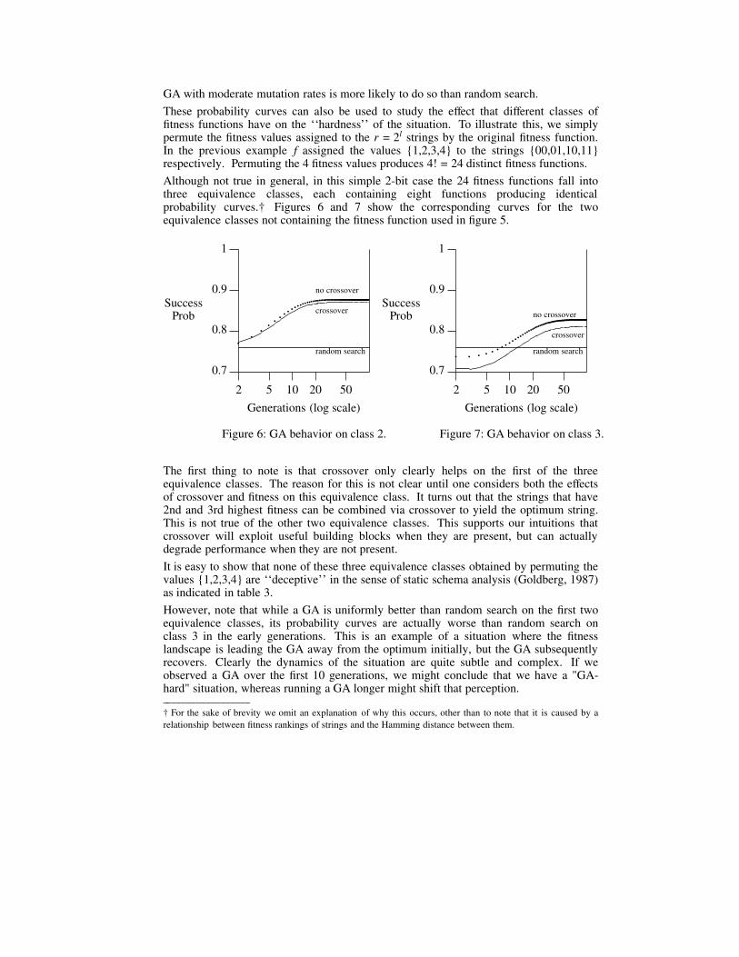
Although not true in general, in this simple 2-bit case the 24 fitness functions fall intothree equivalence classes, each containing eight functions producing identicalprobability curves.† Figures 6 and 7 show the corresponding curves for the twoequivalence classes not containing the fitness function used in figure 5.

2 5 10 20 50

0.7

0.8

0.9

1

SuccessProb

Generations (log scale)

Figure 6: GA behavior on class 2.

••

••

• • • • • • ••••••••••••••••••••••••••••••••••••••••••••••••••••••••••••••••••• ••••••••••••••••••••••

crossover

no crossover

random search

2 5 10 20 50

0.7

0.8

0.9

1

SuccessProb

Generations (log scale)

Figure 7: GA behavior on class 3.

• • • • • • • • • • ••••••••

•••••••••••••••••••••

•••••••••••• •••••••• ••••••••••••••••••••••••••••••••••••••••

crossover

no crossover

random search

The first thing to note is that crossover only clearly helps on the first of the threeequivalence classes. The reason for this is not clear until one considers both the effectsof crossover and fitness on this equivalence class. It turns out that the strings that have2nd and 3rd highest fitness can be combined via crossover to yield the optimum string.This is not true of the other two equivalence classes. This supports our intuitions thatcrossover will exploit useful building blocks when they are present, but can actuallydegrade performance when they are not present.

It is easy to show that none of these three equivalence classes obtained by permuting thevalues {1,2,3,4} are ‘‘deceptive’’ in the sense of static schema analysis (Goldberg, 1987)as indicated in table 3.

However, note that while a GA is uniformly better than random search on the first twoequivalence classes, its probability curves are actually worse than random search onclass 3 in the early generations. This is an example of a situation where the fitnesslandscape is leading the GA away from the optimum initially, but the GA subsequentlyrecovers. Clearly the dynamics of the situation are quite subtle and complex. If weobserved a GA over the first 10 generations, we might conclude that we have a "GA-hard" situation, whereas running a GA longer might shift that perception.__________________

† For the sake of brevity we omit an explanation of why this occurs, other than to note that it is caused by a

relationship between fitness rankings of strings and the Hamming distance between them.

________________________________________________________________________Class Fitness Function Schema Fitness

f(00) f(01) f(10) f(11) f(0*) f(1*) f(*0) f(*1)________________________________________________________________________1 1 2 3 4 1.5 3.5 2.0 3.02 2 1 3 4 1.5 3.5 2.5 2.53 3 1 2 4 2.0 3.0 2.5 2.5________________________________________________________________________������

������

������

������

Table 3: Static schema analysis for the three equivalence classes.

5.3 Dynamic Properties of Deception

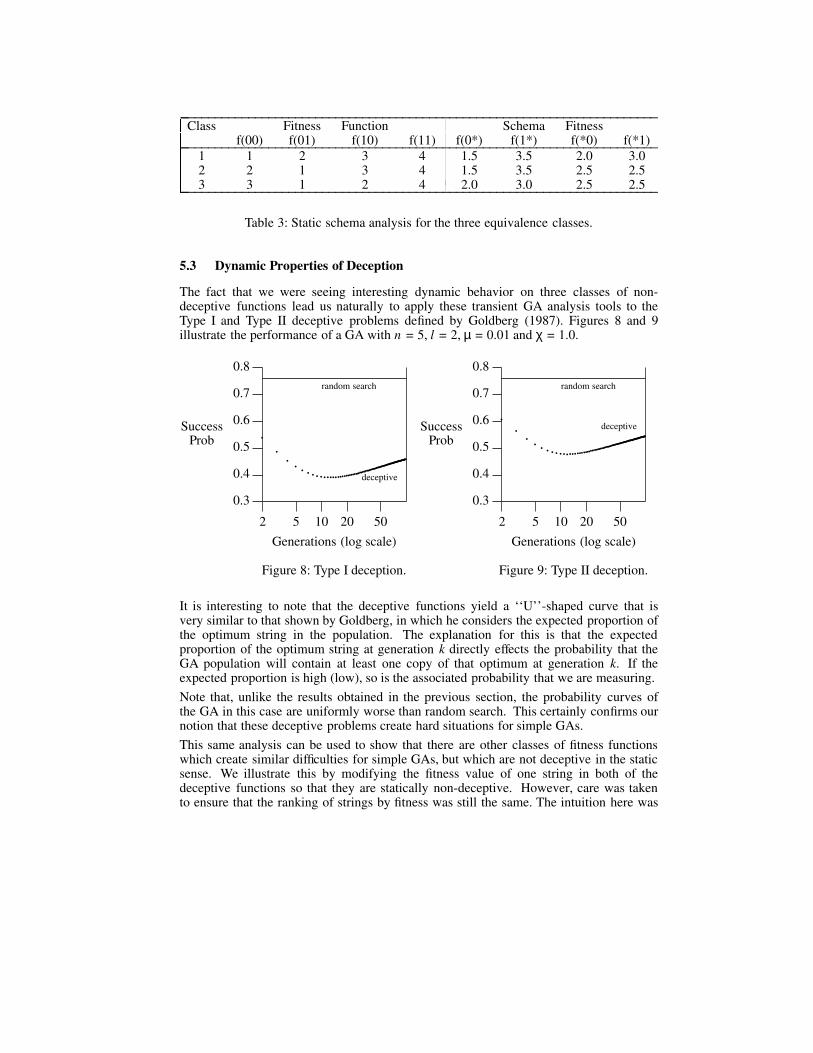
The fact that we were seeing interesting dynamic behavior on three classes of non-deceptive functions lead us naturally to apply these transient GA analysis tools to theType I and Type II deceptive problems defined by Goldberg (1987). Figures 8 and 9illustrate the performance of a GA with n = 5, l = 2, µ = 0.01 and χ = 1.0.

2 5 10 20 50

0.3

0.4

0.5

0.6

0.7

0.8

SuccessProb

Generations (log scale)

Figure 8: Type I deception.

•

••

• • • • • • ••••• •••••••••••••••••••••••••••••

••••••••••••••••••••••••••••••••••••••••••••••••••••••••

deceptive

random search

2 5 10 20 50

0.3

0.4

0.5

0.6

0.7

0.8

SuccessProb

Generations (log scale)

Figure 9: Type II deception.

•

••

• • • • • • • ••• •••••••••••••••••••••••••••••

•••••••••••••••••••••••••••••••••••••••••••••••••••••••••

deceptive

random search

It is interesting to note that the deceptive functions yield a ‘‘U’’-shaped curve that isvery similar to that shown by Goldberg, in which he considers the expected proportion ofthe optimum string in the population. The explanation for this is that the expectedproportion of the optimum string at generation k directly effects the probability that theGA population will contain at least one copy of that optimum at generation k. If theexpected proportion is high (low), so is the associated probability that we are measuring.

Note that, unlike the results obtained in the previous section, the probability curves ofthe GA in this case are uniformly worse than random search. This certainly confirms ournotion that these deceptive problems create hard situations for simple GAs.

This same analysis can be used to show that there are other classes of fitness functionswhich create similar difficulties for simple GAs, but which are not deceptive in the staticsense. We illustrate this by modifying the fitness value of one string in both of thedeceptive functions so that they are statically non-deceptive. However, care was takento ensure that the ranking of strings by fitness was still the same. The intuition here was

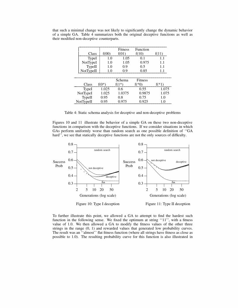
that such a minimal change was not likely to significantly change the dynamic behaviorof a simple GA. Table 4 summarizes both the original deceptive functions as well astheir modified non-deceptive counterparts.

_____________________________________________Fitness Function

Class f(00) f(01) f(10) f(11)_____________________________________________TypeI 1.0 1.05 0.1 1.1

NotTypeI 1.0 1.05 0.975 1.1TypeII 1.0 0.9 0.5 1.1

NotTypeII 1.0 0.9 0.85 1.1_____________________________________________�������

�������

�������

__________________________________________________Schema Fitness

Class f(0*) f(1*) f(*0) f(*1)__________________________________________________TypeI 1.025 0.6 0.55 1.075

NotTypeI 1.025 1.0375 0.9875 1.075TypeII 0.95 0.8 0.75 1.0

NotTypeII 0.95 0.975 0.925 1.0__________________________________________________�������

�������

�������

Table 4: Static schema analysis for deceptive and non-deceptive problems

Figures 10 and 11 illustrate the behavior of a simple GA on these two non-deceptivefunctions in comparison with the deceptive functions. If we consider situations in whichGAs perform uniformly worse than random search as one possible definition of ‘‘GAhard’’, we see that statically deceptive functions are not the only sources of difficulty.

2 5 10 20 50

0.3

0.4

0.5

0.6

0.7

0.8

SuccessProb

Generations (log scale)

Figure 10: Type I deception

•

••

• • • • • • ••••• •••••••••••••••••••••••••••••

••••••••••••••••••••••••••••••••••••••••••••••••••••••••

deceptive

not deceptive

random search

flat

2 5 10 20 50

0.3

0.4

0.5

0.6

0.7

0.8

SuccessProb

Generations (log scale)

Figure 11: Type II deception

•

••

• • • • • • • ••• •••••••••••••••••••••••••••••

•••••••••••••••••••••••••••••••••••••••••••••••••••••••••

deceptivenot deceptive

random search

flat

To further illustrate this point, we allowed a GA to attempt to find the hardest suchfunction in the following sense. We fixed the optimum at string ‘‘11’’, with a fitnessvalue of 1.0. We then allowed a GA to modify the fitness values of the other threestrings in the range (0, 1) and rewarded values that generated low probability curves.The result was an ‘‘almost’’ flat fitness function (where all strings have fitness as close aspossible to 1.0). The resulting probability curve for this function is also illustrated in

figures 10 and 11. Note that the probability curve for this nearly flat fitness function is infact lower than the probability curves for the other four problems in table 4, especially inlater generations. The difficulty with it, of course, is that there is no differential feedbackwhatsoever. On the other hand, if one were measuring difficulty in terms of "best so far"curves, this would certainly look "easy" since near-optimal solutions are abundantalready in the first generation.

Finally, we were curious to see how sensitive these results were to population size, sinceincreasing population size is a standard way to overcome low-order deceptiveness.Figure 12 illustrates typical results obtained with increasing population sizes, confirmingour expectations that the dynamic characteristics of deception remain, but that thedifficulty of the situation (as measured by the probability curves) decreases.

2 5 10 20 50

0.4

0.6

0.8

1

SuccessProb

Generations (log scale)

random search

not deceptive

deceptiveflat

Figure 12: Type II deception with n = 10, µ = 0.01, χ = 1.0

6 WAITING TIME ANALYSIS

The probability curve analysis of the previous section provides some interesting andimportant insights into the non-linear interactions of the various components of a GAFOsituation. However, as we have seen, it doesn’t precisely capture "hardness" in a formthat a GAFO practitioner would necessarily care about. Generally, such a person wouldbe much more interested in ‘‘best so far’’ curves and in knowing how long the GA wouldhave to run on average before first encountering the optimum. In this section we extendthe theory developed in the previous sections to provide exact answers to such questions.

6.1 Expected Waiting Time Theory

The theory extension needed to obtain the expected waiting time until an event ofinterest is first observed is based on the observation that the Q matrix can be used tocompute ‘‘mean first passage times’’ for going from state i to state j (for a nicediscussion of this, see Winston 1991). Questions involving waiting times to convergenceusing a 1-bit Markov model with mutation and selection were considered in the paper by

Goldberg and Segrest (1987). Our work extends these earlier formulations.

More precisely, we wish to compute the length of time that it takes (on the average) toreach state j for the first time, given that the process is currently in state i. Answeringsuch questions involves solving the set of simultaneous equations:

mi, j = Qi, j + k≠jΣ Qi,k (1 + mk, j) (9)

where mi, j denotes the mean first passage time from state i to state j. To understand theequation, consider transitioning from state i to j in one move. This occurs withprobability Qi, j and requires only one step. However, suppose the GA transitions fromstate i to state k, where k is not equal to j. This occurs with probability Qi,k and requiresone step. However, there now remain mk, j steps to state j.

As before, if we are interested in a set J of states, we can compute the mean first passagetime for the GA to first enter that set of states, given that it is currently outside that set:

mi,J = j∈ JΣQi, j +

k∈/ JΣQi,k(1 + mk,J) (10)

where mi,J denotes the mean first passage time from state i to any of the states in set J,and i is not in J. This is very similar to equation 9, with the exception that theprobability of entering state J in one step is simply the sum of the probabilities ofentering each state within J.

Once this system of simultaneous equations is solved, we can calculate the ‘‘expectedwaiting time’’ to reach a state in J, given a random initial state, via:

EWT (J) = i∈ JΣ P(i @ 0) 0 +

i∈/ JΣP(i @ 0) mi,J (11)

There are two parts to Equation 11. The first part reflects the possibility that a randominitial population is in state J, and hence has a zero waiting time. The second partreflects the mean passage time from initial populations not in J, to a state in J. Clearlythis simplifies to:

EWT (J) = i∈/ JΣ P(i @ 0) mi,J (12)

As we noted in section 5, equation 12 hold for any set of states J, and thus can be used toprovide expected waiting times for a variety of "interesting" events such as: the first timean optimum is encountered, the first time the average fitness of the population exceeds agiven threshold, the first time the population diversity falls below a given threshold, etc.

6.2 Expected Waiting Times for GAFOs

Clearly, an interesting GAFO event involves the first time an optimal string is produced.Following the same approach as section 5, we define J to be the set of states containingat least one copy of the optimum string. Then EWT (J) is the expected number ofgenerations until the optimum is first encountered. To us, this scalar quantity is a naturalmeasure of the difficulty of a GAFO situation, with longer EWTs representing moredifficult situations. We explore this view in more detail in this section.

As a starting point, table 5 provides the EWTs for the same three equivalence classes offitness functions studied in section 5 and illustrated in figures 5-7. Recall that in these

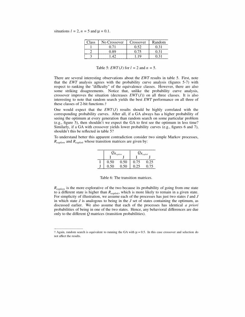
situations l = 2, n = 5 and µ = 0.1.

__________________________________________Class No Crossover Crossover Random__________________________________________

1 0.71 0.52 0.31__________________________________________2 0.89 0.75 0.31__________________________________________3 1.42 1.19 0.31__________________________________________�����

�����

�����

�����

�����

Table 5: EWT (J) for l = 2 and n = 5.

There are several interesting observations about the EWT results in table 5. First, notethat the EWT analysis agrees with the probability curve analysis (figures 5-7) withrespect to ranking the "difficulty" of the equivalence classes. However, there are alsosome striking disagreements. Notice that, unlike the probability curve analysis,crossover improves the situation (decreases EWT (J)) on all three classes. It is alsointeresting to note that random search yields the best EWT performance on all three ofthese classes of 2-bit functions.†

One would expect that the EWT (J) results should be highly correlated with thecorresponding probability curves. After all, if a GA always has a higher probability ofseeing the optimum at every generation than random search on some particular problem(e.g., figure 5), then shouldn’t we expect the GA to first see the optimum in less time?Similarly, if a GA with crossover yields lower probability curves (e.g., figures 6 and 7),shouldn’t this be reflected in table 5?

To understand better this apparent contradiction consider two simple Markov processes,Rexplore and Rexploit whose transition matrices are given by:

_____________________________QRexplore

QRexploit

I J I J_____________________________I 0.50 0.50 0.75 0.25J 0.50 0.50 0.25 0.75_____________________________�����

�����

�����

�����

Table 6: The transition matrices.

Rexplore is the more explorative of the two because its probability of going from one stateto a different state is higher than Rexploit, which is more likely to remain in a given state.For simplicity of illustration, we assume each of the processes has just two states I and Jin which state J is analogous to being in the J set of states containing the optimum, asdiscussed earlier. We also assume that each of the processes has identical a prioriprobabilities of being in one of the two states. Hence, any behavioral differences are dueonly to the different Q matrices (transition probabilities).

__________________

† Again, random search is equivalent to running the GA with µ = 0.5. In this case crossover and selection do

not affect the results.

From equation 4 we have the probability of being in state J at time k given by:

P(J @ k) = sΣ P(s @ 0) Qs,J

k

If we assign equal a priori probabilities to both states, this simplifies to:

P(J @ k) = 0.5 sΣQs,J

k

Since each of the Q matrices are symmetric, so are their powers Qk . Hence theircolumns (as well as their rows) sum to 1.0, leading to a further simplification:

P (J @ k) = 0.5

Hence, in spite of their different transition probabilities, both processes have identicalprobability curves with respect to their likelihood of being in state J at time k, namely, atany given time each process has a 50/50 chance of being in state J.

However, when we calculate expected waiting times until these processes first enter stateJ, we observe something quite different. Using equations 10, we compute the mean firstpassage time from state I to state J for process Rexplore:

mI,J = 0.5 + (0.5)(1.0 + mI,J)

the solution of which yields mI,J = 2.0. The expected waiting time until state J is firstencountered is then easily calculated via equation 12 in which the mean first passagetimes are normalized by the 0.5 probability of being in state I at time zero, yieldingEWTexplore(J) = 1.0.

Similar calculations yield an EWT (J) of 2.0 for Rexploit, producing the curious situationthat, although each process has a 50/50 chance of being in state J at any given instant intime, EWTexplore(J) < EWTexploit(J).

To see why that is the case, consider the sequence of states visited by one of theserandom processes over time:

s1 , s2 , s3 , ..., sk, . . .

Both processes have a 50/50 chance of starting out in state J. If that’s the case, then wehave identical EWT (J)s of zero. However, if both processes start out in state I, thenRexplore is much more likely to switch to state J, resulting in a shorter average waitingtime until the first J occurs in the sequence.

Interestingly, this effect can be made even more dramatic by changing the a prioriprobabilities of being in states I and J. For example, consider the effects of settingP (I @ 0) = 0.25 and P (J @ 0) = 0.75 while keeping the two Q matrices the same asbefore. In this case Pexplore(J @ k) < Pexploit(J @ k) while their relative rankings withrespect to EWT (J) remains unchanged (we omit the proof for the sake of brevity). Thatis, even though Rexplore is less likely to be in state J at any given time than Rexploit is,Rexplore is still more likely to produce the first J because of its higher switching rate.

In summary, this section provides a clear picture of the relative merits of probabilitycurve analysis and EWT analysis. Probability curves provide insight into the dynamicnon-linear interactions of GAFO behavior, but are not good predictors of traditionalmeasures of GAFO performance. EWTs, on the other hand, collapse all of this behaviorinto a single figure of merit which is directly related to the usual notions of GAFOperformance.

6.3 Analyzing GAFO EWTs

If EWT is a useful figure of merit, then it is important to understand how various featuresof GAFO situations affect EWT. Characterizing these effects will in turn provide insights(and make predictions) about how to improve GAFO performance. We present somepreliminary results in this section.

6.3.1 The Importance of Exploration for GAFOs

Finding a balance between exploration and exploitation has been an important theme ofGA research from the very beginning. Achieving such a balance, however, is difficultsince it is a complex non-linear function of selection, representation, operators, andfitness landscape. One of the frequent empirical observations is that GAFO performancecan be improved by using higher mutation rates and more disruptive crossover operators(e.g., uniform crossover) than traditional analysis suggests. The preceding sectionindicates why: EWT measures of performance encourage more exploration thanmeasures involving maximizing total (or average) payoff.

The previous Rexplore-Rexploit example provides an intuitive illustration of how too muchexploitation is bad for EWTs. Table 5, given earlier, provided a more concrete example:for a fixed mutation rate of u = 0.1, adding crossover consistently improved EWT, but inall cases these "traditional" settings were outperformed by random search. Our intuitionwas that, for these simple 2-bit problems, the optimal exploration/exploitation ratio wasmuch higher than we might expect, but that this ratio should decrease as a function of l.

To test this hypothesis, we used EWT analysis to estimate the "optimal" mutation rate (inthe sense of minimizing EWT) for a variety of situations involving the fitness functionf (y) = integer (y) + 1. We kept n = 2 and χ = 1.0, but allowed l to range from 2 to 5.We then estimated the optimal mutation rate by calculating EWT (J) for every µ from0.01 to 0.99, in increments of 0.01. Table 7 gives the optimum µ for each l.

___________________________________________________l 2 3 4 5___________________________________________________

optimal µ 0.68 0.54 0.44 0.36___________________________________________________EWT of GA with optimal µ 1.19 3.25 7.18 14.52___________________________________________________

EWT of RAND (µ=0.5) 1.29 3.26 7.25 15.25___________________________________________________�����

�����

�����

Table 7: Optimum µ for EWT (J) as l increases.

As expected, the advantage of high mutation rates falls off quickly as a function ofincreasing l. Notice also that with these "optimal" mutation rates, the GA is now slightlybetter than random search, but accomplishes this by using much higher levels ofmutation than are typically used. This raises the interesting, but unconfirmed conjecture,that these optimal mutation rates will approach the traditional 1/l heuristic setting as lincreases.

The optimal mutation rates in table 7 that are greater than 0.50 are a bit surprising atfirst. With µ = 1.0 we are essentially complementing each string in the population. Forvery small problems there exists a reasonable chance that the complement of the solutionwill appear in an early generation. Hence, a complement operator can improve EWTs.

As l increases, this effect quickly starts to diminish, although interestingly, a complementoperator can also be quite effective for certain classes of deceptive problems.

6.3.2 Interacting Effects of Crossover and Mutation

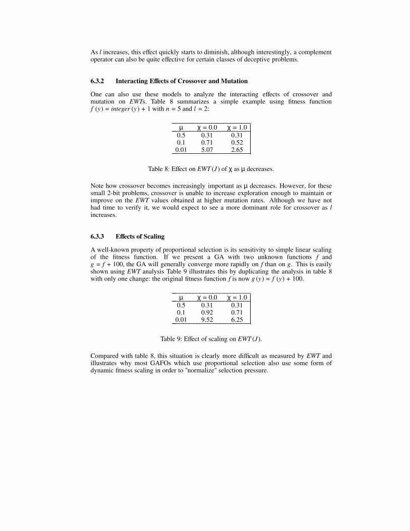
One can also use these models to analyze the interacting effects of crossover andmutation on EWTs. Table 8 summarizes a simple example using fitness functionf (y) = integer (y) + 1 with n = 5 and l = 2:

________________________µ χ = 0.0 χ = 1.0________________________

0.5 0.31 0.310.1 0.71 0.520.01 5.07 2.65________________________�����

�����

�����

Table 8: Effect on EWT (J) of χ as µ decreases.

Note how crossover becomes increasingly important as µ decreases. However, for thesesmall 2-bit problems, crossover is unable to increase exploration enough to maintain orimprove on the EWT values obtained at higher mutation rates. Although we have nothad time to verify it, we would expect to see a more dominant role for crossover as lincreases.

6.3.3 Effects of Scaling

A well-known property of proportional selection is its sensitivity to simple linear scalingof the fitness function. If we present a GA with two unknown functions f andg = f + 100, the GA will generally converge more rapidly on f than on g. This is easilyshown using EWT analysis Table 9 illustrates this by duplicating the analysis in table 8with only one change: the original fitness function f is now g (y) = f (y) + 100.

________________________µ χ = 0.0 χ = 1.0________________________

0.5 0.31 0.310.1 0.92 0.710.01 9.52 6.25________________________�����

�����

�����

Table 9: Effect of scaling on EWT (J).

Compared with table 8, this situation is clearly more difficult as measured by EWT andillustrates why most GAFOs which use proportional selection also use some form ofdynamic fitness scaling in order to "normalize" selection pressure.

6.3.4 Effects of Building Blocks

One can also study the effects of "building blocks" on EWT. To illustrate, we duplicatedthe analysis of table 8 with only one change: the fitness value of f ("01") was increasedby 1. Since the optimum string is "11", the idea was to equally reward both "01" and"10" and set the stage for crossover. Table 10 summarized the results.

________________________µ χ = 0.0 χ = 1.0________________________

0.5 0.31 0.310.1 0.69 0.500.01 5.01 2.45________________________

Table 10: Effect of building blocks on EWT (J).

Clearly, as the mutation rates decrease and crossover plays a more dominant role,rewarding good building blocks uniformly improves EWT (in comparison with table 8).In this particular example the improvements are quite small and one might be tempted toquestion their statistical significance. However, recall that this is not data derived fromempirical averages. These are exact values (subject to rounding errors) computeddirectly from the theory.

7 Summary and Discussion

This paper describes our initial exploration of transient Markov chain analysis as thebasis for a stronger GAFO theory. Although closed form analysis is difficult in general,useful insights can be obtained by means of both visual and computational exploration ofthe transient behavior of the models. We are quite pleased with the initial progress andare optimistic of the future potential of this approach.

There are clearly a number of concerns, primary of which is the scalability of the results.So far, we have observed fairly consistent results as we increase both string length andpopulation size. However, much more work is required to scale up to more realisticvalues of n and l.

There are a variety of directions we are exploring. There are many other visualizationtechniques which have the potential for further elucidation of these models. In additionto expected waiting times, the variance of the waiting times is an important measurewhich can also be derived from the models. It is also possible to study the effects ofother operators (e.g., uniform crossover) and other GA features such as population size,rank selection, and so on.

It would also be nice to see how well fitness correlation (Manderick et al., 1991), whichtakes into account aspects of the fitness function, representation, and the geneticoperators, predicts EWT performance.

An interesting future possibility would be to create Markov models of other evolutionaryalgorithms and standard hill climbers, and then allow a GA to find those problems thatare easy for GAs and hard for hillclimbers (or vice versa), using the EWT performancemeasure!

Acknowledgements

We would like to thank Dr. Daniel Carr for suggesting visualization techniques, and Dr.Marty Fischer for suggestions on Markov Chain analysis.

References

Davis, T. E., & Principe, J. C. (1991) A simulated annealing like convergence theory forthe simple genetic algorithm. Proceedings of the 4th International Conference onGenetic Algorithms, San Diego, 174-181.

De Jong, K. A. (1992) GAs are not function optimizers. Proceedings of the Foundationsof Genetic Algorithms Workshop. Vail, CO: Morgan Kaufmann.

De Jong, K. A. (1975) An analysis of the behavior of a class of genetic adaptive systems.Doctoral Thesis, Department of Computer and Communication Sciences. University ofMichigan, Ann Arbor.

Goldberg, D. E. (1987) Simple genetic algorithms and the minimal, deceptive problem.Chapter 6 in Genetic Algorithms and Simulated Annealing, Lawrence Davis (ed.),Morgan Kaufmann.

Goldberg, D. E., & Segrest, P., (1987) Finite Markov chain analysis of geneticalgorithms. Proceedings of the 2nd International Conference on Genetic Algorithms,Cambridge, 1-8.

Holland, J. H. (1975) Adaptation in natural and artificial systems. Ann Arbor, Michigan:The University of Michigan Press.

Horn, J. (1993) Finite Markov chain analysis of genetic algorithms with niching.Proceedings of the 5th International Conference on Genetic Algorithms, San Mateo, CA:Morgan Kaufmann, 110-117.

Horn, J., Goldberg, D. E., & Deb, K., (1994) Implicit niching in a learning classifiersystem: nature’s way. Evolutionary Computation, Volume 2, #1, 37-66.

Juliany, J., & Vose, M. D., (1994) The genetic algorithm fractal. To appear inEvolutionary Computation, Volume 2, #1.

Manderick, B., de Weger, M., & Spiessens, P., (1991) The genetic algorithm and thestructure of the fitness landscape. Proceedings of the 4th International Conference onGenetic Algorithms, San Diego, 143-150.

Mafoud, S. (1993) Finite Markov chain models of an alternative selection strategy forthe genetic algorithm. Complex Systems, 7 (2), 155-170.

Nix, A. E., & Vose, M. D., (1992) Modelling genetic algorithms with Markov chains.Annals of Mathematics and Artificial Intelligence #5, 79 - 88.

Rudolph, G. (1994) Massively parallel simulated annealing and its relation toevolutionary algorithms. Evolutionary Computation, Volume 1, #4.

Suzuki, J. (1993) A Markov chain analysis on a genetic algorithm. Proceedings of the5th International Conference on Genetic Algorithms, Urbana-Champaign, 146-153.

Vose, M. (1992) Modeling simple genetic algorithms. Proceedings of the Foundations ofGenetic Algorithms Workshop, Vail, CO: Morgan Kaufmann, 63-74.

Whitley, D. (1992) An executable model of a simple genetic algorithm, Proceedings ofthe Foundations of Genetic Algorithms Workshop, Vail, CO: Morgan Kaufmann, 45-62.

Winston, W. (1991) Operations Research: Applications and Algorithms, 2nd Edition,PWS-Kent Publishing Company, Boston MA.