Using Manometers to Precisely Measure

Pressure, Flow and Level

Precision Measurement Since 1911

• .. A1eriam Instrument l lrl [ a Scott Fetzer compaii]

Table of Contents

Manometer Principles .... ... ......... ..... ..................... ..... .... :. 2

Indicating Fluids .. .......... ...... ...... .... .. ..... ..... .... ... .. ....... ... ... 5

Manometer Corrections ...... ............................... ... .......... 6

Digital Manometers ...................................... .. ............. .... 9

Applications Guide .. ........... .. ..... ... ...... ..... .-..... ........ .. ... .. 12

Glossary of Pressure Terms ... .... .. ................................. 16

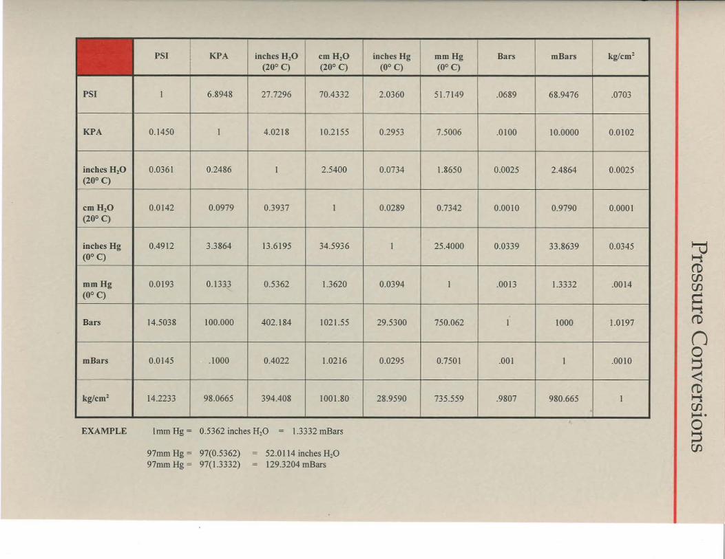
Pressure Conversions .............. ..... ..... Inside Back Cover

1

Manometer Principles

The manometer, one of the earliest pressure measur­ing instruments, when used properly is very accurate. NIST recognizes the U tube manometer as a primary standard due to its inherent accuracy and simplicity of operation. The manometer has no moving parts sub­ject to wear, age, or fatigue. Manometers operate on the Hydrostatic Balance Principle: a liquid column of known height will exert a known pressure when the weight per unit volume of the liquid is known. The fundamental relationship for pressure expressed by a liquid column is

p = differential pressure P 1 = pressure at the low pressure connection P2 = pressure at the high pressure connection p density of the liquid g acceleration of gravity h height of the liquid column

In all forms of manometers (U tubes, well-types, and inclines) there are two liquid surfaces. Pressure deter­minations are made by how the fluid moves when pressures are applied to each surface. For gauge pres­sure, P2 is equal to zero (atmospheric reference), simplifying the equation to

p= pgh

U TUBE MANOMETERS

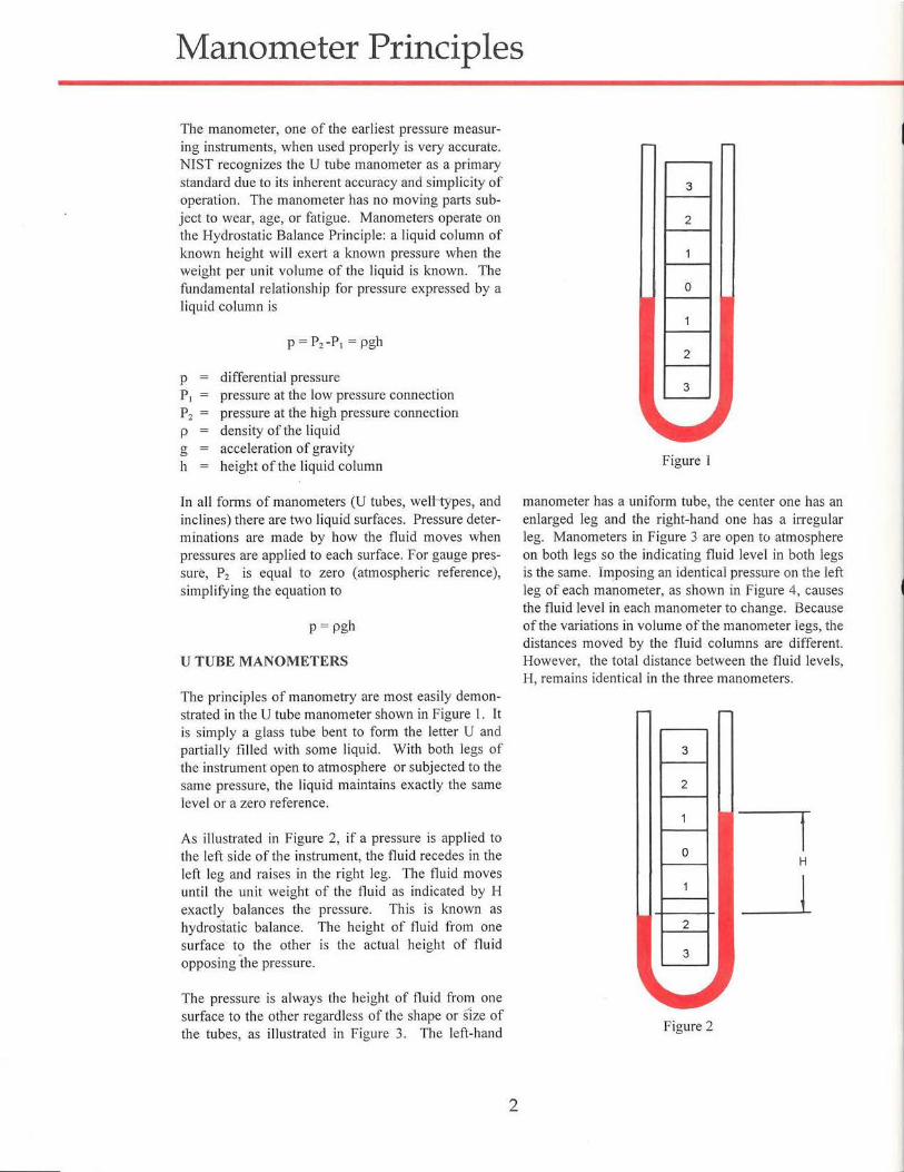
The principles of manometry are most easily demon­strated in the U tube manometer shown in Figure l. It is simply a glass tube bent to form the letter U and partially filled with some liquid. With both legs of the instrument open to atmosphere or subjected to the same pressure, the liquid maintains exactly the same level or a zero reference.

As illustrated in Figure 2, if a pressure is applied to the left side of the instrument, the fluid recedes in the left leg and raises in the right leg. The fluid moves until the unit weight of the flu id as indicated by H exactly balances the pressure. This is known as hydrostatic balance. The height of fluid from one surface to the other is the actual height of fluid opposing the pressure.

The pressure is always the height of fluid from one surface to the other regardless of the shape or Size of the tubes, as illustrated in Figure 3. The left-hand

2

3

2

1

0

1

2

3

Figure 1

manometer has a uniform tube, the center one has an enlarged leg and the right-hand one has a irregular leg. Manometers in Figure 3 are open to atmosphere on both legs so the indicating fluid level in both legs is the same. Imposing an identical pressure on the left leg of each manometer, as shown in Figure 4, causes the fluid level in each manometer to change. Because of the variations in volume of the manometer legs, the distances moved by the fluid columns are different. However, the total distance between the fluid levels, H, remains identical in the three manometers.

3

2

0 I H

_j_ 2

3

Figure 2

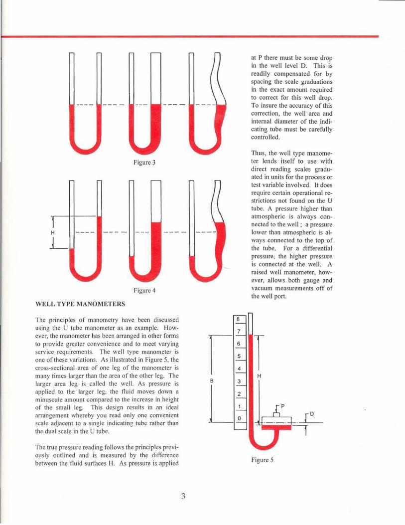
Figure 3

H

L

Figure 4

WELL TYPE MANOMETERS

The principles of manometry have been discussed us ing the U tube manometer as an example. How­ever, the manometer has been arranged in other forms to provide greater convenience and to meet vary ing service requirements. The well type manometer is one of these variations. As illustrated in Figure 5, the cross-sectional area of one leg of the manometer is many times larger than the area of the other leg. The larger area leg is called the well. As pressure is applied to the larger leg, the fluid moves down a minuscule amount compared to the increase in height of the small leg. This des1gn results m an ideal arrangement whereby you read only one convenient scale adjacent to a smgle indicating tube rather than the dual scale in the U tube.

The true pressure reading follows the principles previ­ously outlined and is measured by the difference between the nuid surfaces H. As pressure is appl ied

3

at P there must be some drop in the well level D. This is readily compensated for by spacing the scale graduations in the exact amount required to correct for this well drop. To insure the accuracy of this correction, the well area and internal diameter of the indi­cating tube must be carefully controlled.

Thus, the well type manome­ter lends itself to use with direct reading scales gradu­ated in units for the process or test variable involved. lt does require certain operational re­strictions not found on the U tube. A pressure higher than atmospheric is always con­nected to the well ; a pressure lower than atmospheric is al­ways connected to the top of the tube. For a differential pressure, the higher pressure is connected at the well. A raised well manometer, how­ever, allows both gauge and vacuum measurements off of the well port.

Figure 5

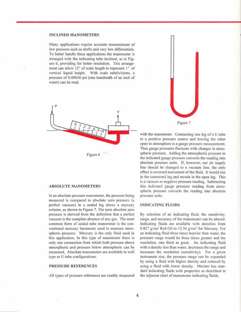
INCLINED MANOMETERS

Many applications require accurate measurement of low pressure such as drafts and very low differentials. To better handle these applications the manometer is arranged with the indicating tube inclined, as in Fig­ure 6, providing for better resolution. This arrange­ment can allow 12" of scale length to represent 1" of vertical liquid height. With scale subdivisions, a pressure of 0.00036 psi (one hundredth of an inch of water) can be read.

Figure 6 -......__

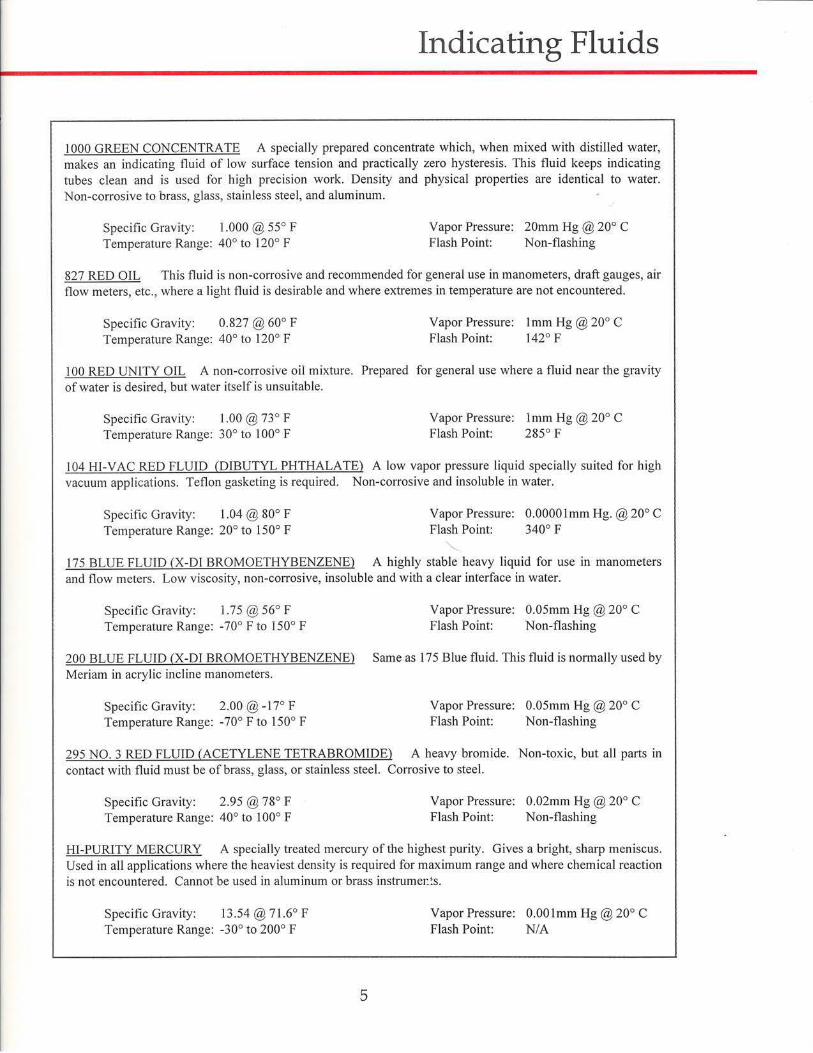
ABSOLUTE MANOMETERS

In an absolute pressure manometer, the pressure being measured is compared to absolute zero pressure (a perfect vacuum) in a sealed leg above a m((rcury column, as shown in Figure 7. The term absolute zero pressure is derived from the definition that a perfect vacuum is the complete absence of any gas. The most common form of sealed tube manometer is the con­ventional mercury barometer used to measure atmo­spheric pressure. Mercury is the only fluid used in this application. In this type of manometer there is only one connection from wh ich both pressure above atmospheric and pressure below atmospheric can be measured. Absolute manometers are available in well type or U tube configurations.

PRESSURE REFERENCES

All types of pressure references are readily me~sured

4

Figure 7

with the manometer. Connecting one leg of a U tube to a positive pressure source and leaving the other open to atmosphere is a gauge pressure measurement. Thus gauge pressures fluctuate with changes in atmo­spheric pressure. Adding the atmospheric pressure to the indicated gauge pressure converts the reading into absolute pressure units. ff, however, our air supply line should be changed to a vacuum line, the only effect is reversed movement of the fluid. It would rise in the connected leg and recede in the open leg. This is a vacuum or negative pressure reading. Subtracting this indicated gauge pressure reading from atmo­spheric pressure converts the reading into absolute pressure uni ts.

INDICATING FLUIDS

By selection of an indicating fluid, the sensitivity, range, and accuracy of the manometer can be altered. Indicating fluids are available with densities from 0.827 glcm3 Red Oil to 13.54 glcm3 for Mercury. For an indicating fluid three times heavier than water, the pressure range would be three times greater and the resolution, one third as great. An indicating fluid with a density less than water, decreases the range and increases the resolution (sensitivity). For a given instrument size, the pressure range can be expanded by using a fluid with higher density and reduced by using a fluid with lower density. Meriam has stan­dard indicating fluids with properties as described in the adjacent chart of manometer indicating fluids.

Indicating Fluids

1 000 GREEN CONCENTRATE A specially prepared concentrate which, when mixed with distilled water, makes an indicating fluid of low surface tension and practically zero hysteresis. This fluid keeps indicating tubes clean and is used for high precision work. Density and physical properties are identical to water. Non-corrosive to brass, glass, stainless steel, and aluminum.

Specific Gravity: t .000 @ 55° F Vapor Pressure: 20mm Hg@ 20° C Temperature Range: 40° to 120° F Flash Point: Non-flashing

827 RED OIL This fluid is non-corrosive and recommended for general use in manometers, draft gauges, air flow meters, etc., where a light fluid is desirable and where extremes in temperature are not encountered.

Specific Gravity: 0.827@ 60° F Vapor Pressure: lmm Hg@ 20° C Temperature Range: 40° to 120° F Flash Point: 142° F

I 00 RED UNITY OIL A non-corrosive oil mixture. Prepared for general use where a fluid near the gravity of water is desired, but water itself is unsuitable.

Specific Gravity: 1.00 @ 73° F Temperature Range: 30° to t 00° F

Vapor Pressure: l mm Hg@ 20° C Flash Point: 285° F

I 04 HI-V AC RED FLUJD (DIBUTYL PHTHALATE) A low vapor pressure liquid specially suited for high vacuum applications. Teflon gasketing is required. Non-corrosive and insoluble in water.

Specific Gravity: 1.04 @ 80° F Temperature Range: 20° to 150° F

Vapor Pressure: 0.0000 lmm Hg. @ 20° C Flash Point: 340° F

175 BLUE FLUID (X-DI BROMOETHYBENZENE) A highly stable heavy liquid for use in manometers and flow meters. Low viscosity, non-corrosive, insoluble and with a clear interface in water.

Specific Gravity: 1.75 @ 56° F Temperature Range: -70° F to 150° F

200 BLUE FLUID (X-DI BROMOETHYBENZENE) Meriam in acrylic incline manometers.

Specific Gravity: 2.00 @ -17° F Temperature Range: -70° F to 150° F

Vapor Pressure: 0.05mm Hg@ 20° C Flash Point: Non-flashing

Same as 175 Blue fluid. This fluid is normally used by

Vapor Pressure: 0.05mm Hg@ 20° C Flash Point: Non-flashing

295 NO. 3 RED FLUID (ACETYLENE TETRABROMlDE) A heavy bromide. Non-toxic, but all parts in contact with fluid must be of brass, glass, or stainless steel. Corrosive to steel.

Specific Gravity: 2.95 @ 78° F Temperature Range: 40° to 1 00° F

Vapor Pressure: 0.02mm Hg @ 20° C Flash Point: Non-flashing

HI-PURITY MERCURY A specially treated mercury of the highest purity. Gives a bright, sharp meniscus. Used in all applications where the heaviest density is required for maximum range and where chemical reaction is not encountered. Cannot be used in aluminum or brass instrumec~.

Specific Gravity: 13.54 @ 71.6° F Vapor Pressure: O.OOlmm Hg@ 20° C Temperature Range: -30° to 200° F Flash Point: N/ A

5

Manometer Corrections

As simp le as manometry is, certain aspects are often overlooked. Manometry measurements are fu nctions of both density and gravity. The values of these two are not constant. Density is a function of temperature, and gravity is a funct ion of latitude and e levation. Because of this relationship specific ambient condi­tions must be selected as standard, so that a fixed definition for pressure can be maintained.

Standard conditions for mercury:

Density 13.595 1 g/cm3.

at oo C (32° F)

Gravity 980.665 cm/sec2 (32.174 ft/sec2)

at sea level and 45.544 degrees latitude

Standard conditions fo r water:

Density 1.000 g/cm3

at 4° C (39.2° F)

Gravity 980.665 em/sec 2 (32.174 ft/sec2)

at sea level and 45.544 degrees latitude

The universal acceptance of a standard for water has been slow. Meriam has chosen 4° C as its standard. This temperature has been chosen due to the density being 1.000 g/cm3. Other institutions have chosen different standards, for instance in aeronautics 15° C (59° F) is used. The American Gas Association uses 15.6° C (60° F). The Instrument Society of America (ISA) has chosen 20° C (68° F) as its standard.

Recogn izing that manometers may be read outside standard temperature and gravity, corrections should be applied to improve the accuracy of a manometer reading at any given condition.

FLUID DENSITY CORRECTION

Manometers indicate the correct pressure at only one temperature. This is because the indicating fluid den­s ity changes with temperature. If water is the indicat­ing flu id, an inch scale indicates one inch of water at 4° C only. On the same scale mercury indicates one inch of m~rcury at oo C only. A reading using water or mercury taken at 20° C (68° F) is not an accurate reading. The error introduced is about 0.4% of read­ing for mercury and about 0.2% of reading for water. S ince manometers are used at temperatures above and below the standard temperature, corrections are

6

needed. A simple way of correcting fo r density changes is to ratio the densities.

h,

Po

p,

(Standard) Pogho=(Ambient) p, gh,

corrected height of the indicating fluid to standard temperature height of the indicating fluid at the temperature when read densit;,; of the indicating fluid at standard tern perature density of the indicating fluid at the temperature when read

This method is very accurate, when density/tempera­ture relations are known. Data is readily available for water and mercury.

Density (g/cm3) as a function of temperature (0 C) for

mercury is

13.556786 (I- 0.0001818(T - 15.5556))

Density (g/cm3) as a function of temperature (0 C) for

water is

0.9998395639 + 6.798299989xl0-5 (T) -9.1 0602556x 1 0·6(T2)+ 1.005272999x I o-7 (T3)

-1.126713526x 1 0·9(T')+6.59l795606x I o-'2 (T5)

For other fluids , manometer scales and fluid densities may be formulated to read inches of water or mercury at a set temperature. This temperature is usually ambient temperature. This decreases the error due to temperature change, because most manometers are used at or close to ambient temperatures. Tn some work direct readings close to design temperature are accurate enough. The manometer still only reads correct at one temperature, and for precise work the temperature corrections cannot be overlooked. Tem­perature versus density data can be supplied for a ll Meriam indicating fluids.

GRAVITY CORRECTION

The need for gravity correction arises because gravity at the location of the instrument governs the weight of the liquid column. Like the temperature correction, gravity correction is a ratio.

(Standard) p0 &,ho = (Ambient) p,g,h,

h0 = g,p, X h,

&>Po

g., standard gravity- 980.665 cm/s2 (45.54°N latitude and sea level)

g, gravity at the instruments location

A I 0° change in latitude at sea level will introduce approximately 0.1% error in reading. At the Equator (0°) the error is approximately 0.25% . An increase in e levation of 5000 ft. wi ll introduce an error of ap­proximately 0.05% .

Gravity values have been determined by the U.S. Coast and Geodetic Survey at many points in the United States. Using these values, the U.S. Geodetic Survey can interpolate to determine a gravity value sufficient for most work. To obtain a gravity report, the instruments latitude, longitude, and elevation are needed. For precise work you must have the value of the gravity measured at the instrument location.

Where a high degree of accuracy is not necessary and

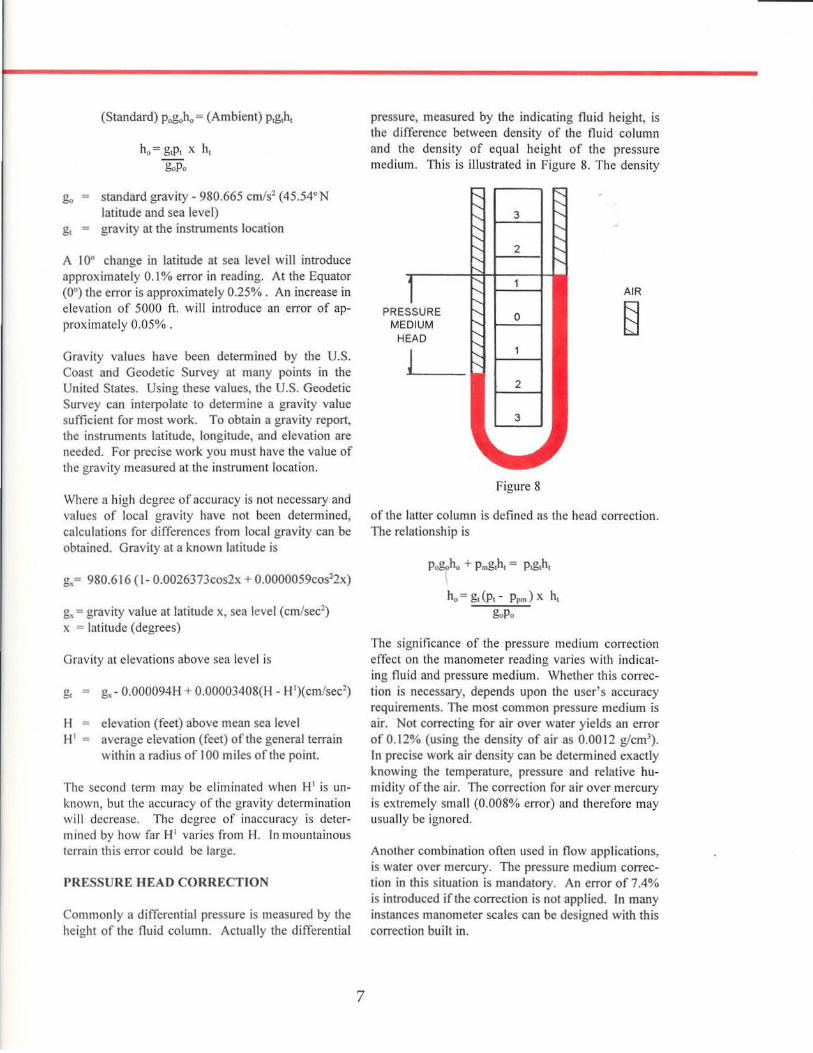
pressure, measured by the indicating fluid height, is the difference between density of the fluid column and the density of equal height of the pressure medium. This is illustrated in Fig ure 8. The density

AIR

§

Figure 8

values of local gravity have not been determined, of the latter column is defined as the head correction. calculations for differences from local gravity can be The relationship is obtained. Gravity at a known latitude is

g,= 980.616 ( 1- 0.0026373cos2x + 0.0000059cos22x)

g,= gravity value at latitude x, sea level (cm/sec2)

x = latitude (degrees)

Gravity at elevations above sea level is

g, g.- 0.000094H + 0.00003408(H- H1)(cm/sec2)

H elevation (feet) above mean sea level H1 = average elevation (feet) of the general terrain

within a radius of I 00 miles of the point.

The second term may be eliminated when W is un­known , but the accuracy of the gravity determination will decrease. The degree of inaccuracy is deter­mined by how far H1 varies from H. In mountainous terrain this error could be large.

PRESSURE HEAD CORRECTION

Commonly a differential pressure is measured by the height of the fluid column. Actually the differential

7

ho= g,(p,- Ppm) X h,

&>Po

The significance of the pressure medium correction effect on the manometer reading varies with indicat­ing fluid and pressure medium. Whether this correc­tion is necessary, depends upon the user's accuracy requirements. The most common pressure medium is air. Not correcting for air over water yields an error of 0.12% (using the density of air as 0.0012 g/cm3).

In precise work air density can be determined exactly knowing the temperature, pressure and relative hu­midity of the air. The corTection for air over mercury is extremely small (0.008% error) and therefore may usually be ignored.

Another combination often used in flow applications, is water over mercury. The pressure medium correc­tion in this situation is mandatory. An error of 7.4% is introduced if the correction is not applied. In many instances manometer scales can be designed with this correction built in.

SCALE CORRECTION

As with the indicating fluids, temperature changes affect the scale. At higher temperatures the scale will expand and the graduations will be further apart. The opposite effect will occur at lower temperatures. All Meriam scales are fabricated at a 22° C (71.6° F) temperature. A ten degree C shift in temperature from that at which the scale was manufactured will induce an error in the reading of about 0.023% in an aluminum scale. All Meriam scales are made of a lu­minum . This correction may be ignored when work­ing within ± I 0° C of the temperature at which the scale was manufactured.

a coefficient of expansion for the scale material 0.0000232/°C for aluminum

T temperature when the manometer was read T0 temperature when the scale was manufactured

COMPRESSIBILITY /

Compressibility of indicating fluids is negligible ex­cept in a few applications. For compressibility to have an effect, the manometer must be used in mea­suring high differential pressures. At high differential pressures the fluid shrinkage (increase in density) may begin to be resolvable on the manometer. At 250 psi the density of water changes approximately 0.1 %. Depending upon accuracy requirements compressibil­ity may or may not be critical. The relationship between pressure and density fo r water is

p = 0.000003684p+ 0.9999898956

p density of water (g.cm3) at 4 ° C and pressure p

p pressure in psia

Since the need to correct is very rare, other indicating fluid's compressiblities have not been determined. Mercury' s compressibility is negligible.

ABSORBED GASES

Absorbed gases are those gases found dissolved in a liquid. The pressure of dissolved gases decreases the density of the liquid. Air is a commonly dissolved gas that is absorbed by most manometer fluids. The density error of water fully saturated with air is .00004% at 20° C. The effect is variable and requires

8

consideration for each gas in contact with a particular fluid. Mercury is one exception in which absorbed gases are not found. This makes mercury an excellent manometer fluid in vacuum and absolute pressure applications. Along with mercury, Meriam produces 104 Hi-Vac Red Fluid (Dibutyl Phthalate- l.04g/cm3

@ 80° F). This fluid has a very low vapor pressure (0.0000 I mm Hg). This makes it a good choice as an indicating fluid for vacuum applications. The low vapor pressure prevents the loss of fluid from evapo­ration and in some instances prevents contamination from condensation of the indicating fluid in the test set-up. It cannot be used in absolute units, because it absorbs gases easily.

CAPILLARY CONSlDERATJONS

Capillary effects occur due to the surface tension or wetting characteristics between the liquid and the glass tube. As a result of surface tension or wetting, most fluids form a convex meniscus. Mercury is the only indicating fluid which does not wet the glass and consequently, forms a concave meniscus. For consis­tent results, you must always observe the fluid menis­cus in the same way, whether convex or concave. To help reduce the effects of surface tension, manome­ters should be designed with large bore tubes. This flattens the meniscus, making it easier to read. A large bore tube also helps fluid drainage. The larger the bore the smaller the time lag while drainage occurs. Another controlling factor is the accumula­tion of corrosion and dirt on the liquid surface. The presence of foreign material changes the shape of the meniscus. With mercury it also helps to tap or v ibrate the tube to reduce error in the readings. A final note to capillary effects is the addition of a wetting agent to the manomter fluid. Adding the wetting agent helps in obtaining a symmetrical meniscus. This decreases the difficulty in making readings. A wetting agent is not needed with all fluids but is added to Meriam 1000 Green Concentrate.

ACCURACY

A typical water manometer has an accuracy of 0.1 inches of water, a manometer w ith a vernier has an accuracy of 0 .01 inches of water, while a manometer equiped with a micrometer can provide an accuracy of 0.002 inches of water.

What is an inch of water? The correct answer to this question has taken on increased importance with the demand for better accuracy and the introduction of digital manometers. For example, lets assume that you have just received your new digital manometer and you decide to verify its accuracy. The manufac­turer claims 0.1% accuracy at 100 inches of water. You set up a test using a deadweight tester and a water manometer. After placing a 100 inch of water weight on the deadweight tester, you record a reading of 99.8 inches of water on the digital manometer and l 00.2 inches of water on the manometer. Which is right? The answer to this question will be evident after the following discussion of manometers and dead weight testers and their relationship to digital manometers. There will also be a discussion of digital manometer accuracy and resolution.

Manometers - The manometer is considered a pri­mary standard since the pressure exerted by the liquid column can be accurately determined by the measure­ment of basic physical properties: the height of the column and the density of the liquid. For a manometer filled with water the pressure equation is

g, g., Pa Pw = Po h =

P = (g/go)(Pw - Pa)h

Po

gravity at instrument location standard gravity (980.665 cm/sec2

)

density of air at observed temperature density of water at observed temperature density of water at standard temperature height of water column in inches

Notice that in order to determine the pressure indi­cated by the height of a water column one needs to know more than the height of the column. Both the local gravity and the density of the manometer fluid and the fluid being measured, in this case water and air, need to be known. As can be seen, the pressure indicated by an inch of water varies with location and temperature. In order to make the readings compara­ble they must be reported at the same temperature and gravity. The three commonly used reference condi­tions for water columns are shown on the table below.

Standard Temperature Gravity

Scientific 4° C (39.2° F) 980.665 AGA 15.6° C (60° F) 980.665 Industrial 20° C (68° F) 980.665

9

Digital Manometers

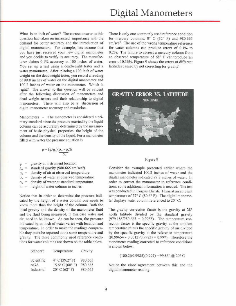
There is only one commonly used reference condition for mercury columns: 0° C (32° F) and 980.665 cm/sec2

• The use of the wrong temperature reference for water columns can produce errors of 0.1% to 0.2%. The failure to correct a mercury co lumn from an observed temperature of 68° F can · prpduce an error of 0.36%. Figure 9 shows the errors at different latitudes caused by not correcting for gravity.

Figure 9

Consider the example presented earlier where the manometer indicated 100.2 inches of water and the digital manometer indicated 99.8 inches of water. In order to correct the manometer to reference condi­tions, some additional infonnation is needed. The test was conducted in Corpus Christi, Texas at an ambient temperature of27° C (80.6° F). The digital manome­ter displays water column referenced to 20° C.

The gravity correction factor is the gravity at 28° north latitude divided by the standard gravity (979.185/980.665 = 0.9985). The temperature cor­rection factor is the specific gravity at the ambient temperature minus the specific gravity of air divided by the specific gravity at the reference temperature ((0.99654- 0.0012)/0.9983) = 0.997). Therefore the manometer reading corrected to reference conditions is shown below.

(100.2)(0.9985)(0.997) = 99.85" @ 20° c

Notice the close agreement between this and the dig ital manometer reading .

\

The use of a water manometer is not practical for field calibrations since a manometer with a range of I 00 inches of water would be over 8 feet tall. A solution to this problem is to substitute a heavy liquid, such as mercury, for the water and to adjust the scale to read in inches of water. This reduces the scale by a factor of 13.59, the ratio of the specific gravity of mercury to that of water. Although this reduces the scale length to less than 8 inches, it also reduces the scale resolution and therefore its accuracy. Typical accu­racy for this type of manometer is 0.25 inches of water. This type of manometer can be read directly only at the conditions for wh ich the scale was calcu­lated. A typical scale would read inches of water referenced to 4° C when observed at 22° C at a gravity of 980.665 cm/sec2

• Corrections must be calculated if any of the conditions vary from those at which the scale was calculated. The manometer is an accurate pressure indicating device if the specific gravity of the manometer fluid is accurately known and the correction factors are properly applied.

Dead Weight Tester - Dead weight testers are the most accurate pressure sources available. Unlike manometers that measure pressure, dead weight testers generate accurate pressures. The pneumatic dead weight tester balances a known weight on a co lumn of air from a nozzle of known area. Since the weight and the area can be accurately measured, the pressure generated can be determined by dividing the weight by the area. The dead weight tester is consid­ered a primary standard since both weight and area are properties that can be easily and accurately mea­sured. Dead weight testers with accuracies of 0.015% are readily available.

Dead weight testers also require corTection factors to determine the actual pressure generated. In the evalu­ation example presented earlier, the digital manome­ter and the manometer are in agreement at 99.8 inches of water but the dead weight tester has a 100 inches of water weight. Dead weight testers are calibrated at a set of reference conditions. In this case the reference conditions are 20° C and 980.665 cm/sec2. Because the dead weight is operating at a different gravity, the same gravity correction must be applied to the dead weight tester as to the manometer.

(100)(0.9985) = 99.85" @ 20° c

Notice that after applying the correction factors all three of the instruments agree within their specified

accuracies. If the reference temperature were 15.6° C additional correction factors would have to be applied to the dead weight tester and the manometer. Dead weight testers can be calibrated at different tempera­ture references and gravities. The certificate of cali­bration for the dead weight tester will indicate the reference conditions used for its calibration.

Since dead weight testers do not indicate the pressure output one must be sure that there are no leaks in the system. A leak will cause the pressure at the instru­ment under test to be lower then that indicated by the weights. A dead weight tester is a precision piece of equipment and should be carefully maintained and operated in a clean environment to insure its accu­racy. Because of its high accuracy, the dead weight tester is the recommended pressure source for evalu­ating digital manometers.

EVALUATING DIGITAL MANOMETERS

The digital manometer is a recent addition to field calibration instrumentation. These instruments are light weight, approximately I pound, and are avail­able with accuracies from 0.2% to 0.025%. Their accuracy places them between the manometer and the dead weight tester, while their size and weight make them more convenient for field calibration. Most available instruments have a 3 1

/ 2 or 41/ 2 digit display

with resolution down to 0.01 inches ofwater. Digital manometers are not primary standards and their accu­racy should be verified periodically against a primary standard. When digital manometers are calibrated with properly corrected primary standards they re­quire no further correction to indicate within their stated accuracy.

10

The evaluation of a digital manometer begins by comparing the manufacturer's published accuracy rat­ings. This is not as simple as it appears, since there is no standard format for accuracy statements. For example, one manufacturer may include the tempera­ture coefficient of enor in the accuracy rating by specifying the accuracy over a specific temperature range while another manufacturer may state the tem­perature coefficient separately. To compare these specifications, the temperature error would have to be calculated over the operating temperature range and added to tue accuracy rating. Compare the following:

0. 1% F.S. 0 - 40°C 0.1% F.S. + 0.0 l %/°C

Although both units are 0.1% F.S. the latter un it is within this limit only at its calibration temperature of 20° C. To equate the two we must multiply the temperature coefficient by the temperature difference between 20° C and 40° C ((0.0 1 )(20) = 0.2%). Adding this to the 0. 1% accuracy at 20° C yields an accuracy of 0.3% F.S. over the temperature range of 0° C to 40° C. Therefore, the first unit is more accurate than the second unit. Always look for a statement of temperature effect. All pressure indica­tors are affected by temperature and manufacturers use various methods to minimize these effects. The manufacturer that does not document temperature effect is either unaware of it or unwilling to make it known to the consumer.

The accuracy rating indicates the limit that errors will not exceed when the instrument is operated under the specified conditions. An accuracy rating normally includes linearity, hysteresis and dead band. If the specifications state the accuracy components sepa­rately, then they must be combined to determine the total accuracy rating. The method recommended by the Instrument Society of America is to take the square root of the sum of the squares of the accuracy components. Since the accuracy rating is stated at specified cond itions, your evaluation tests must be conducted under the same conditions. For example, if the accuracy is specified at 70° F then the evaluation tests should be conducted at that temperature; other­wise an additional error factor may be introduced by the temperature coefficient of accuracy.

Accuracy can be expressed in several d ifferent ways. Among them are

Percent of span Percent of fu II scale Percent of reading

The tightest method of expressing accuracy is percent of reading while the most common is percent of full scale. An instrument with a range of 200 inches of water and an accuracy rating of 0.1% of fu ll scale will have an error of +/-0.2 inches of water at any reading. Therefore, at 10 inches of water, the error would be 0.2 inches of water or 2% of reading. The actual error at each test point wil l have to be calculated before proceeding with the evaluation.

Resolution is a very important specification in digita-l instruments. Reso lution is defined as the smallest

11

increment that can be distinguished or displayed. The following relationship exists between accuracy and resolution: resolution can exceed accuracy but accu­racy can not exceed resolution. A 31/ 2 digit instru­ment divides the input signal into 1999 parts. The smallest increment that can be displayed · is 1 part in 1999 or 0.05% of full scale. This would limit the accuracy of this instrument to 0.05% of fu ll scale. Although decreasing the resolution will decrease the accuracy of the instrument, increasing the resolution will not increase the accuracy. For example, a 0.05% of full scale instrument with a 4 1

/ 2 digit display has a resolution of 0.005% of full scale, since the accuracy does not change, the additional digit provided by the increased resolution is meaningless. Do not assume that all displayed digits are significant; compare the accuracy to the resolution to determine how many digits are significant.

After determining the error limits for each test point, the instrument evaluation can proceed. An instrument or pressure source with an accuracy of between 3 and 10 times that of the instrument under evaluation should be used. A dead weight tester with an accuracy of 0.0 15% of reading is recommended. If the evalua­tion is being conducted in inches of water, then the following informafion must be known: the reference temperature at which the dead weight tester was calibrated; and the reference temperature at which the instrument was calibrated. This is very important since the indicated error between different reference temperatures can be as much as 0.2%. In addition, all appropriate correction factors, especially gravity, must be applied to the dead weight tester and there must be no leaks in the system.

The minimum number of recommended test points is two. These should be at 50% and 100% of each range of the instrument. A more stringent test would in­volve four test points, at 25%, 50%, 75% and I 00% of each range. A full ten point test is usually not required to evaluate an instrument, but it does provide the most detailed information about the instrument.

The digital pressure indicator is an ideal instrument for field calibration of transmitters and recorders. It is lightweight, accurate, and easy to use. The selection of an acceptable instrument can be simplified with an understanding of accuracy specifications. The eva lu­ation of an instrument's accuracy requires a thorough knowledge of the primary standard used and the correction factors required.

Applications Guide

PRESSURE TRANSMITTER CALIBRATION

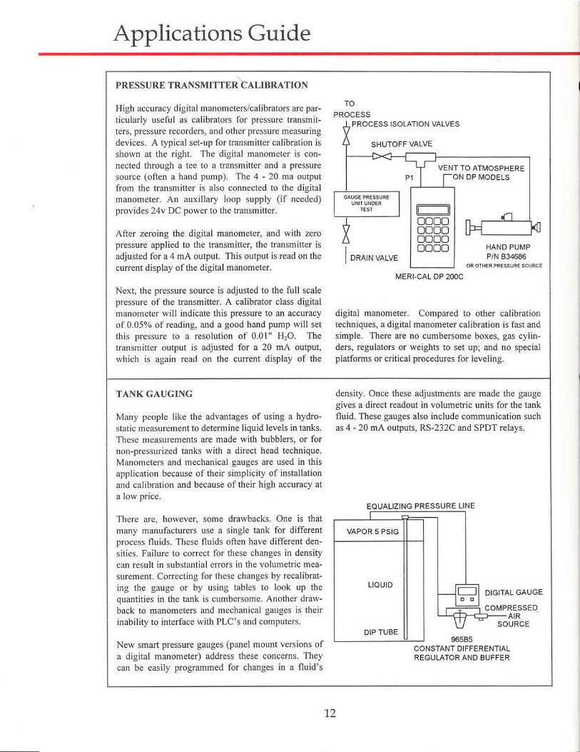
High accuracy digital manometers/calibrators are par­ticularly useful as calibrators for pressure transmit­ters, pressure recorders, and other pressure measuring devices. A typical set-up for transmitter calibration is shown at the right. The digital manometer is con­nected through a tee to a transmitter and a pressure source (often a hand pump). The 4 - 20 rna output from the transmitter is also connected to the digital manometer. An auxiliary loop supply (if needed) provides 24v DC power to the transmitter.

After zeroing the digital manometer, and with zero pressure applied to the transmitter, the transmitter is adjusted for a 4 rnA output. This output is read on the current display of the digital manometer.

Next, the pressure source is adjusted to the full scale pressure of the transmitter. A calibrator class digital manometer will indicate this pressure to an accuracy of 0.05% of reading, and a good hand pump will set this pressure to a resolution of 0.01" H20. The transmitter output is adjusted for a 20 mA output, which is again read on the current display of the

TANK GAUGING

Many people like the advantages of using a hydro­static measurement to determine liquid levels in tanks. These measurements are made with bubblers, or for non-pressurized tanks with a direct head technique. Manometers and mechanical gauges are used in this application because of their simplicity of installation and calibration and because of their high accuracy at a low price.

There are, however, some drawbacks. One is that many manufacturers use a single tank for different process fluids. These fluids often have different den­sities. Failure to correct for these changes in density can result in substantial errors in the volumetric mea­surement. Correcting for these changes by recalibrat­ing the gauge or by using tables to look up the quantities in the tank is cumbersome. Another draw­back to manometers and mechanical gauges is their inability to interface with PLC's and computers.

New smart pressure gauges (panel mount versions of a digital manometer) address these concerns. They can be easily programmed for changes in a fluid's

TO

PROCESS ~?PROCESS ISOLATION VALVES

l.l SHUTOFF VALVE

~CK~~~--~----------~ "" v VENT TO ATMOSPHERE

P1 I roN DP MODELS

~~-------. ~--~~ GAUGE PRESSURE I

UNIT UNDER TEST

I DRAIN VALVE

II II 0000 0000 0000 0000 HAND PUMP

P/N B34686 OR OTHER PRESSURE SOURCE

MERI-CAL DP 200C

digital manometer. Compared to other calibration techniques, a digital manometer calibration is fast and simple. There are no cumbersome boxes, gas cylin­ders, regulators or weights to set up; and no special platforms or critical procedures for leveling.

density. Once these adjustments are made the gauge gives a direct readout in volumetric units for the tank fluid. These gauges also include communication such as 4 - 20 rnA outputs, RS-232C and SPDT relays.

12

EQUALIZING PRESSURE LINE I

VAPOR 5 PSIG

LIQUID

DIP TUBE

K~ DIGITALGAUGE

_l COMPRESSE~ L...J..-QD--L::::r-- AIR

\!) ""tT' SOURCE

965B5 CONSTANT DIFFERENTIAL REGULATOR AND BUFFER

AIR FLOW

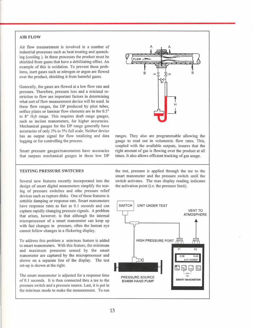
Air flow measurement is involved in a number of industrial processes such as heat treating and quench­ing (cooling). In these processes the product must be shielded from gases that have a debilitating effect. An example of this is oxidation. To prevent these prob­lems, inert gases such as nitrogen or argon are flowed over the product, shielding it from harmful gases.

Generally, the gases are flowed at a low flow rate and pressure. Therefore, pressure loss and a minimal re­striction to flow are important factors in determining what sort of flow measurement device will be used. In these flow ranges, the DP produced by pitot tubes, orifice plates or laminar flow elements are in the 0.5'' to 8" H20 range. This requires draft range gauges, such as incline manometers, for higher accuracies. Mechanical gauges for the DP range generally have accuracies of only 3% to 5% full scale. Neither device has an output signal for flow totalizing and data logging or for controlling the process.

Smart pressure gauges/manometers have accuracies that surpass mechanical gauges in these low DP

TESTING PRESSURE SWITCHES

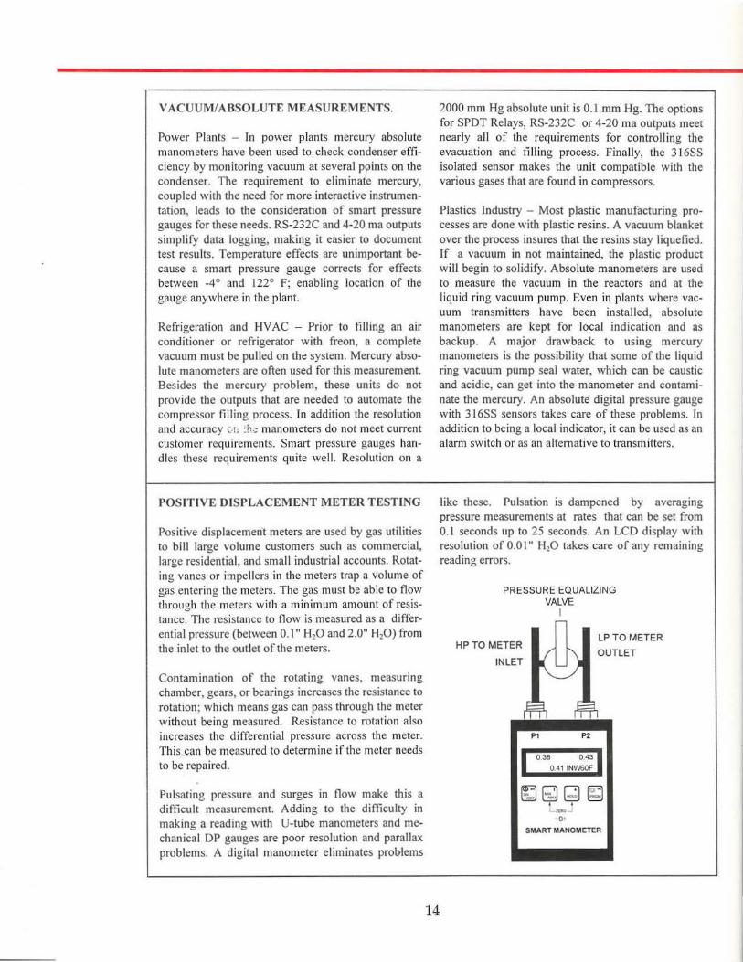
Several new features recently incorporated into the design of smart digital manometers simplify the test­ing of pressure switches and othe pressure relief devices such as rupture disks. One of these features is settable damping or response rate. Smart manometers have response rates as fast as 0.1 seconds and can capture rapidly changing pressure signals. A problem that arises, however, is that although the internal microprocessor of a smart manometer can keep up with fast changes in pressure, often the human eye cannot follow changes in a flickering display.

To address this problem a minimax feature is added to smart manometers. With this feature, the minimum and maximum pressures sensed by the smart manometer are captured by the microprocessor and shown on a separate line of the display. The test set-up is shown at the right.

The smart manometer is adjusted for a response time of 0.1 seconds. It is then connected thru a tee to the pressure switch and a pressure source. Last, it is put in the min/max mode to make the measurement. To run

13

A A

ranges. They also are programmable allowing the gauge to read out in volumetric flow rates. This, coupled with the available outputs, insures that the right amount of gas is flowing over the product at all times. It also allows efficient tracking of gas usage.

the test, pressure is applied through the tee to the smart manometer and the pressure switch until the switch activates. The max display reading indicates the activation point (i.e. the pressure limit).

UNIT UNDER TEST

HIGH PRESSURE PORT

PRESSURE SOURCE 834686 HAND PUMP

VENT TO ATMOSPHERE

,_,_, t ()o

SMART MANOMETER

VACUUM/ABSOLUTE MEASUREMENTS.

Power Plants - In power plants mercury absolute manometers have been used to check condenser effi­ciency by monitoring vacuum at several points on the

I

condenser. The requirement to eliminate mercury, coupled with the need for more interactive instrumen­tation, leads to the consideration of smart pressure gauges for these needs. RS-232C and 4-20 rna outputs simplify data logging, making it easier to document test results. Temperature effects are unimportant be­cause a smart pressure gauge corrects for effects between -4° and .122° F; enabling location of the gauge anywhere in the plant.

Refrigeration and HVAC - Prior to filling an air conditioner or refrigerator with freon, a complete vacuum must be pulled on the system. Mercury abso­lute manometers are often used for this measurement. Besides the mercury problem, these units do not provide the outputs that are needed to automate the compressor filling orocess. In addition the resolution and accuracy ;:.r, ~h.; manometers do not meet current customer requirements. Smart pressure gauges han­dles these requirements quite well. Resolution on a

POSITIVE DISPLACEMENT METER TESTING

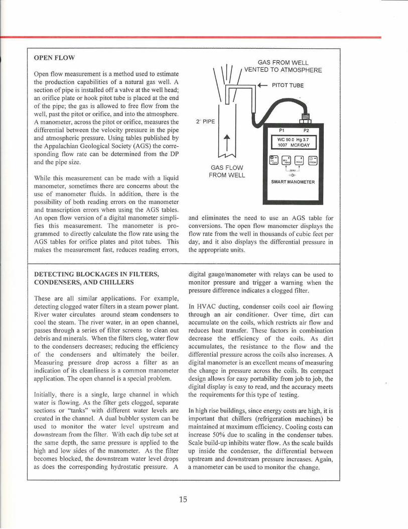
Positive displacement meters are used by gas utilities to bill large volume customers such as commercial, large residential, and small industrial accounts. Rotat­ing vanes or impellers in the meters trap a volume of gas entering the meters. The gas must be able to flow through the meters with a minimum amount of resis­tance. The resistance to flow is measured as a differ­ential pressure (between 0.1" H20 and 2.0" H20) from the inlet to the outlet of the meters.

Contamination of the rotating vanes, measuring chamber, gears, or bearings increases the resistance to rotation; which means gas can pass through the meter without being measured. Resistance to rotation also increases the differential pressure across the meter. This can be measured to determine if the meter needs to be repaired.

Pulsating pressure and surges in flow make this a difficult measurement. Adding to the difficulty in making a reading with U-tube manometers and me­chanical DP gauges are poor resolution and parallax problems. A digital manometer eliminates problems

2000 mm Hg absolute unit is 0.1 mm Hg. The options for SPDT Relays, RS-232C or 4-20 rna outputs meet nearly all of the requirements for controlling the evacuation and fi lling process. Finally, the 316SS isolated sensor makes the unit compatible with the various gases that are found in compressors.

Plastics Industry - Most plastic manufacturing pro­cesses are done with plastic resins. A vacuum blanket over the process insures that the resins stay liquefied. If a vacuum in not maintained, the plastic product will begin to solidify. Absolute manometers are used to measure the vacuum in the reactors and at the liquid ring vacuum pump. Even in plants where vac­uum transmitters have been installed, absolute manometers are kept for local indication and as backup. A major drawback to using mercury manometers is the possibility that some of the liquid ring vacuum pump seal water, which can be caustic and acidic, can get into the manometer and contami­nate the mercury. An absolute digital pressure gauge with 316SS sensors takes care of these problems. In addition to being a local indicator, it can be used as an alarm switch or as an alternative to transmitters.

14

like these. Pulsation is dampened by averaging pressure measurements at rates that can be set from 0.1 seconds up to 25 seconds. An LCD display with resolution of 0.0 I" H20 takes care of any remaining reading errors.

PRESSUREEQUAU~NG VALVE

HPTO METER

INLET

P1

I -

P2

LP TO METER

OUTLET

I 0.38 0.43 1 0.41 INWSOF

SMART MANOMETER

OPEN FLOW

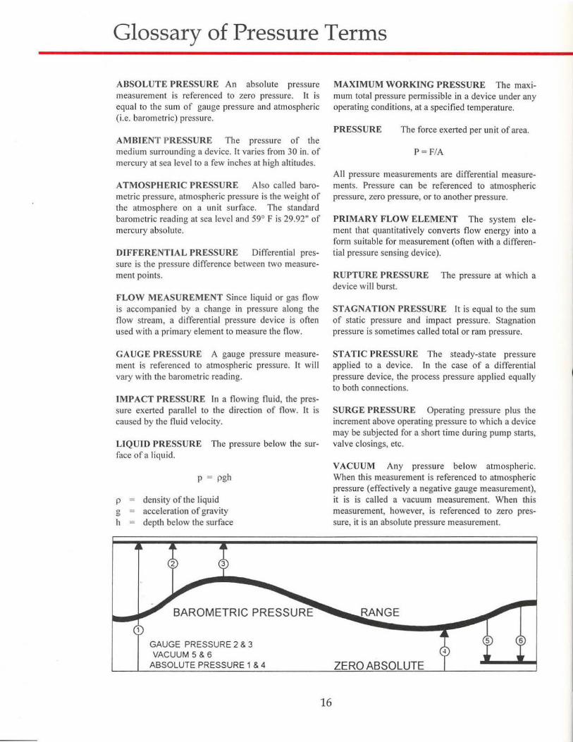
Open flow measurement is a method used to estimate the production capabilities of a natural gas well. A section of pipe is installed off a valve at the well head; an orifice plate or hook pitot tube is placed at the end of the pipe; the gas is allowed to free flow from the well, past the pitot or orifice, and into the atmosphere. A manometer, across the pitot or orifice, measures the differential between the velocity pressure in the pipe and atmospheric pressure. Using tables published by the Appalach ian Geological Society (AGS) the corre­sponding flow rate can be determined from the DP and the pipe size.

While this measurement can be made with a liquid manometer, sometimes there are concerns about the use of manometer fluids. In addition, there is the possibility of both reading errors on the manometer and transcription errors when using the AGS tables. An open flow version of a digital manometer simpli­fies this measurement. The manometer is pro­grammed to directly calculate the flow rate using the AGS tables for orifice plates and pitot tubes. This makes the measurement fast, reduces reading errors,

DETECTING BLOCKAGES lN FILTERS, CONDENSERS, AND CHILLERS

These are all similar applications. For example, detecting clogged water fi lters in a steam power plant. River water circulates around steam condensers to cool the steam. The river water, in an open channel, passes through a series of filter screens to clean out debris and minerals. When the filters clog, water flow to the condensers decreases; reducing the efficiency of the condensers and ultimately the boiler. Measuring pressure drop across a filter as an indication of its c lean liness is a common manometer application. The open channel is a special problem.

Initially, there is a single, large channel in which water is flowing. As the filter gets clogged, separate sections or " tanks" with different water levels are created in the channel. A dual bubbler system can be used to monitor the water level upstream and downstream from the filter. With each dip tube set at the same depth, the same pressure is appl ied to the high and low sides of the manometer. As the fi lter becomes blocked, the downstream water level drops as does the corresponding hydrostatic pressure. A

15

GAS FROM WELL VENTED TO ATMOSPHERE

2 .. PIPE

GAS FLOW FROM WELL -t Ot-

SMART MANOMETER

and eliminates the need to use an AGS table for conversions. The open flow manometer displays the flow rate from the well in thousands of cubic feet per day, and it also displays the differential pressure in the appropriate units.

digital gauge/manometer with relays can be used to monitor pressure and trigger a warning when the pressure difference indicates a clogged filter.

In HV AC ducting, condenser coils cool air flowing through an air conditioner. Over time, dirt can accumulate on the coils, which restricts air flow and reduces heat transfer. These factors in combination decrease the efficiency of the coils. As dirt accumulates, the resistance to the flow and the differential pressure across the coils also increases. A digital manometer is an excellent means of measuring the change in pressure across the coils. Its compact desig_n allows for easy portability from job to job, the digital display is easy to read, and the accuracy meets the requirements for this type of testing.

fn high rise buildings, since energy costs are high, it is impo1tant that chillers (refrigeration machines) be maintained at maximum efficiency. Cooling costs can increase 50% due to scaling in the condenser tubes. Scale build-up inhibits water flow. As the scale builds up inside the condenser, the differential between upstream and downstream pressure increases. Again, a manometer can be used to monitor the change.

Glossary of Pressure Terms

ABSOLUTE PRESSURE An abso lute pressure measurement is referenced to zero pressure. It is equal to the sum of gauge pressure and atmospheric (i .e. barometric) pressure.

AMBIENT PRESSURE The pressure of the medium surrounding a device. It varies from 30 in. of mercury at sea level to a few inches at high altitudes.

ATMOSPHERIC PRESSURE Also called baro­metric pressure, atmospheric pressure is the weight of the atmosphere on a unit surface. The standard barometric read ing at sea level and 59° F is 29.92" of mercury absolute.

DJFFERENTIAL PRESSURE Differential pres­sure is the pressure difference between two measure­ment points.

FLOW MEASUREMENT Since liquid or gas now is accompanied by a change in pressure along the flow stream, a differential pressure device is often used with a primary element to measure the now.

GAUGE PRESSURE A gauge pressure measure­ment is referenced to atmospheric pressure. It will vary with the barometric reading.

IMPACT PRESSURE In a flowing fluid, the pres­sure exerted parallel to the direction of now. lt is caused by the fluid velocity.

LIQUID PRESSURE The pressure below the sur­face of a liquid.

p g h

p = pgh

density of the liquid acceleration of gravity depth below the surface

GAUGE PRESSURE 2 & 3 VACUUM 5 & 6

ABSOLUTEPRESSURE1&4

16

MAXIMUM WORKING PRESSURE The maxi­mum total pressure permissible in a device under any operating conditions, at a specified temperature.

PRESSURE The force exerted per unit of area.

P = F/A

All pressure measurements are differential measure­ments. Pressure can be referenced to atmospheric pressure, zero pressure, or to another pressure.

PRIMARY FLOW ELEMENT The system ele­ment that quantitatively convetts flow energy into a form suitable for measurement (often with a differen­tial pressure sensing device).

RUPTURE PRESSURE The pressure at which a device will burst.

STAGNATION PRESSURE It is equal to the sum of static pressure and impact pressure. Stagnation pressure is sometimes called total or ram pressure.

STATIC PRESSURE The steady-state pressure applied to a device. In the case of a differential pressure device, the process pressure applied equally to both connections.

SURGE PRESSURE Operating pressure plus the increment above operating pressure to which a device may be subjected for a short time during pump starts, valve closings, etc.

VACUUM Any pressure below atmospheric. When this measurement is referenced to atmospheric pressure (effectively a negative gauge measurement), it is is called a vacuum measurement. When this measurement, however, is referenced to zero pres­sure, it is an absolute pressure measurement.

RANGE

ZERO ABSOLUTE

PSI

KPA

inches H20 (20° C)

cmH20 (20° C)

inches Hg (00 C)

mm Hg (00 C)

Bars

mBars

kglcm2

EXAMPLE

PSI KPA inches H20 em H20 (20° C) (20° C)

I 6.8948 27.7296 70.4332

0.1450 I 4.0218 10.2155

0.0361 0.2486 I 2.5400

0.0142 0.0979 0.3937 I

0.4912 3.3864 13.6195 34.5936

0.0193 0.1333 0.5362 1.3620

14.5038 100.000 402.184 1021.55

0.0145 .1000 0.4022 1.0216

14.2233 98.0665 394.408 1001.80

1mm Hg = 0.5362 inches H20 = 1.3332 mBars

97mm Hg = 97(0.5362) 97mm Hg = 97(1.3332)

52.0114 inches H20 129.3204 mBars

inches Hg mmHg Bars mBars kg/cm2

(00 C) (00 C)

2.0360 51.7149 .0689 68.9476 .0703

0.2953 7.5006 .0100 10.0000 0.0102

0.0734 1.8650 0.0025 2.4864 0.0025

0.0289 0.7342 0.0010 0.9790 0.0001

I 25.4000 0.0339 33.8639 0.0345

0.0394 I .0013 1.3332 .0014

29.5300 750.062 1 1000 1.0197

0.0295 0.7501 .001 I .0010

28.9590 735.559 .9807 980.665 1

•

/ \

-

• M .IMeriam Instrument [ a Seott Fetzer com~

10920 Madison Avenue • Cleveland, OH 44102 Telephone 216-281-1100 • FAX: 216-281-0228

15M 4/97 File No. 050:MHB-1

-