Using Logic in the Generation of Referring Expressions · Using Logic in the Generation of...

Using Logic in the Generation of ReferringExpressions

Carlos Areces1, Santiago Figueira?2, and Daniel Gorın3

1 INRIA Nancy, Grand Est, [email protected]

2 Departamento de Computacion, FCEyN, UBA and CONICET, Argentina3 Departamento de Computacion, FCEyN, UBA, Argentina

{santiago,dgorin}@dc.uba.fr

Abstract. The problem of generating referring expressions (GRE) isan important task in natural language generation. In this paper, weadvocate for the use of logical languages in the output of the contentdetermination phase (i.e., when the relevant features of the object tobe referred are selected). Many different logics can be used for this andwe argue that, for a particular application, the actual choice shall con-stitute a compromise between expressive power (how many objects canbe distinguished), computational complexity (how difficult it is to deter-mine the content) and realizability (how often will the selected contentbe realized to an idiomatic expression). We show that well-known resultsfrom the area of computational logic can then be transferred to GRE.Moreover, our approach is orthogonal to previous proposals and we illus-trate this by generalizing well-known content-determination algorithmsto make them parametric on the logic employed.

1 Generating Referring Expressions

The generation of referring expressions (GRE) –given a context and an elementin that context generate a grammatically correct expression in a given naturallanguage that uniquely represents the element– is a basic task in natural languagegeneration, and one of active research (see [4,5,6,20,8] among others). Most of thework in this area is focused on the content determination problem (i.e., findinga collection of properties that singles out the target object from the remainingobjects in the context) and leaves the actual realization (i.e., expressing a givencontent as a grammatically correct expression) to standard techniques4.

However, there is yet no general agreement on the basic representation ofboth the input and the output to the problem; this is handled in a rather ad-hocway by each new proposal instead.

Krahmer et al. [17] make the case for the use of labeled directed graphs in thecontext of this problem: graphs are abstract enough to express a large number of

? S. Figueira was partially supported by CONICET (grant PIP 370) and UBA (grantUBACyT 20020090200116).

4 For exceptions to this practice see, e.g., [16,21]

2 Carlos Areces, Santiago Figueira, and Daniel Gorın

domains and there are many attractive, and well-known algorithms for dealingwith this type of structures. Indeed, these are nothing other than an alternativerepresentation of relational models, typically used to provide semantics for formallanguages like first and higher-order logics, modal logics, etc. Even valuations,the basic models of propositional logic, can be seen as a single-pointed labeledgraph. It is not surprising then that they are well suited to the task.

In this article, we side with [17] and use labeled graphs as input, but we arguethat an important notion has been left out when making this decision. Exactlybecause of their generality, graphs do not define, by themselves, a unique notionof sameness. When do we say that two nodes in the graphs can or cannot bereferred uniquely in terms of their properties? This question only makes senseonce we fix a certain level of expressiveness which determines when two graphs,or two elements in the same graph, are equivalent.

Expressiveness can be formalized using structural relations on graphs (iso-morphisms, etc.) or, alternatively, logical languages. Both ways are presentedin §2, where we also discuss how fixing a notion of expressiveness impacts on thenumber of instances of the GRE problem that have a solution; the computationalcomplexity of the GRE algorithms involved; and the complexity of the surfacerealization problem. We then investigate the GRE problem in terms of differentnotions of expressiveness. We first explore in §3 how well-known algorithms fromcomputational logic can be applied to GRE. This is a systematization of the ap-proach of [1], and we are able to answer a complexity question that was left openthere. In §4 we take the opposite route: we take the well-known GRE-algorithmof [17], identify its underlying expressivity and rewrite in term of other logics.We then show in §5 that both approaches can be combined and finally discuss in§6 the size of an RE relative to the expressiveness employed. We conclude in §7with a short discussion and prospects for future work.

2 Measuring Expressive Power

Relational structures are very suitable for representing situations or scenes. Arelational structure (also called “relational model”) is a non-empty set of objects–the domain– together with a collection of relations, each with a fixed arity.

Formally, assume a fixed and finite (but otherwise arbitrary) vocabulary ofn-ary relation symbols.5 A relational model M is a tuple 〈∆, || · ||〉 where ∆ isa nonempty set, and || · || is a suitable interpretation function, that is, ||r|| ⊆ ∆n

for every n-ary relation symbol r in the vocabulary. We say that M is finitewhenever ∆ is finite. The size of a modelM is the sum #∆+ #|| · ||, where #∆is the cardinality of ∆ and #|| · || is the sum of the sizes of all relations in || · ||.

Figure 1 below shows how we can represent a scene as a relational model.Intuitively, a, b and d are dogs, while c and e are cats; d is a small beagle; b andc are also small. We read sniffs(d, e) as “d is sniffing e”.

Logical languages are fit for the task of (formally) describing elements ofa relational structure. Consider, e.g., the classical language of first-order logic

5 Constants and function symbols can be represented as relations of adequate arity.

Using Logic in the Generation of Referring Expressions 3

∆ = {a, b, c, d, e}||dog || = {a, b, d}||cat || = {c, e}

||beagle|| = {d}||small || = {b, c, d}||sniffs|| = {(a, a), (b, a), (c, b), (d, e), (e, d)}

a

dog

b

dogsmall

c

catsmall

d

dogbeaglesmall

e

cat

sniffs

sniffs sniffs

sniffs

sniffs

Fig. 1. Graph representation of scene S.

(with equality), FO, given by:

> | xi 6≈ xj | r(x) | ¬γ | γ ∧ γ′ | ∃xi.γ

where γ, γ′ ∈ FO, r is an n-ary relation symbol and x is an n-tuple of variables.As usual, γ ∨ γ′ and ∀x.γ are short for ¬(¬γ ∧ ¬γ′) and ¬∃x.¬γ, respectively.Formulas of the form >, xi 6≈ xj and r(x) are called atoms.6 Given a relationalmodel M = 〈∆, || · ||〉 and a formula γ with free variables7 among x1 . . . xn, weinductively define the extension or interpretation of γ as the set of n-tuples||γ||n ⊆ ∆n that satisfy:

||>||n = ∆n ||xi 6≈ xj ||n = {a | a∈∆n, ai 6= aj}||¬δ||n = ∆n \ ||δ||n ||r(xi1 . . . xik)||n = {a | a∈∆n, (ai1 . . . aik)∈||r||}||δ ∧ θ||n = ||δ||n ∩ ||θ||n ||∃xl.δ||n = {a | ae ∈ ||δ′||n+1 for some e}

where 1 ≤ i, j, i1, . . . , ik ≤ n, a = (a1 . . . an), ae = (a1 . . . an, e) and δ′ is obtainedby replacing all occurrences of xl in δ by xn+1. When the cardinality of the tuplesinvolved is known from the context we will just write ||γ|| instead of ||γ||n.

With a language syntax and semantics in place, we can now formally definethe problem of L-GRE for a target set of elements T (we slightly adapt thedefinition in [1]):

L-GRE Problem

Input: a model M = 〈∆, || · ||〉 and a nonempty target set T ⊆ ∆.Output: a formula ϕ ∈ L such that ||ϕ|| = T if it exists, and ⊥ otherwise.

When the output is not ⊥, we say that ϕ is an L-referring expression (L-RE)for T in M. Simply put then, the output of the L-GRE problem is a formulaof L whose interpretation in the input model is the target set, if such a formulaexists. This definition applies also to the GRE for objects of the domain bytaking a singleton set as target.

6 For technical reasons, we include the inequality symbol 6≈ as primitive. Equality canbe defined using negation.

7 W.l.o.g. we assume that no variable appears both free and bound, that no variableis bound twice, and that the index of bound variables in a formula increases fromleft to right.


By using formulas with n free variables one could extend this definition todescribe n-ary relations; but here we are only interested in describing subsets ofthe domain. Actually, we shall restrict our attention a little further:

Convention 1. We will only consider relational models with unary and binaryrelation symbols (i.e., labeled graphs). We will consistently use p for a unaryrelation symbol (and called it a proposition) and r for a binary relation symbol.

This convention captures the usual models of interest when describing scenes asthe one presented in Figure 1. Accommodating relations of higher arity in ourtheoretical framework is easy, but it might affect computational complexity.

2.1 Choosing the Appropriate Language

Given a model M, there might be an infinite number of formulas that uniquelydescribe a target (even formulas which are not logically equivalent might havethe same interpretation once a model is fixed). Despite having the same inter-pretation in M, they may be quite different with respect to other parameters.

As it is well known in the automated text generation community, different re-alizations of the same content might result in expressions which are more or lessappropriate in a given context. Although, as we mentioned in the introduction,we will only address the content determination part (and not the surface real-ization part) of the GRE problem, we will argue that generating content usinglanguages with different expressive power can have an impact in the posteriorsurface generation step.

Let us consider again the scene in Figure 1. Formulas γ1–γ4 shown in Table 1are all such that γi uniquely describes b (i.e., ||γi|| = {b}) in model S. Arguably,γ1 can be easily realized as “the small dog that sniffs a dog”. Syntactically, γ1 ischaracterized as a positive, conjunctive, existential formula (i.e., it contains nonegation and uses only conjunction and existential quantification). Expressionswith these characteristics are, by large, the most commonly found in corporaas those compiled in [22,9,7]. Formula γ2, on the other hand, contains negation,disjunction and universal quantification. It could be realized as “the small dogthat only sniffs things that are not cats” which sounds unnatural. Even a smallchange in the form of γ2 makes it more palatable: rewrite it using ∃, ¬, and ∧to obtain “the small dog that is not sniffing a cat”. Similarly, γ3 and γ4 seemcomputationally harder to realize than γ1: γ3 contains an inequality (“the dogsniffing another dog”), while the quantified object appears in the first argumentposition in the binary relation in γ4 (“the dog that is sniffed by a small cat”).

Summing up, we can ensure, already during the content determination phase,certain properties of the generated referring expression by paying attention tothe formal language used in the representation. And we can do this, even beforetaking into account other fundamental linguistics aspects that will make certainrealization preferable like saliency, the cognitive capacity of the hearer (can sherecognize a beagle from another kind of dog?), etc.

As a concrete example, let FO− be the fragment of FO-formulas where theoperator ¬ does not occur (but notice that atoms xi 6≈ xj are permitted). By


γ1 : dog(x) ∧ small(x) ∧ ∃y.(sniffs(x, y) ∧ dog(y))

γ2 : dog(x) ∧ small(x) ∧ ∀y.(¬cat(y) ∨ ¬sniffs(x, y))

γ3 : dog(x) ∧ ∃y.(x 6≈ y ∧ dog(y) ∧ sniffs(x, y))

γ4 : dog(x) ∧ ∃y.(cat(y) ∧ small(y) ∧ sniffs(y, x))

Table 1. Alternative descriptions for object b in the model shown in Figure 1.

restricting content determination to FO−, we ensure that formulas like γ2 willnot be generated. If we ban 6≈ from the language, γ3 is precluded.

The fact that the representation language used has an impact on contentdetermination is obvious, but it has not received the attention it deserves. Are-ces et al. [1] use different description logics (a family of formal languages usedin knowledge representation, see [2]) to classify, and give a formal framework toprevious work on GRE. Let us quickly introduce some of these languages as wewill be mentioning them in future sections. Using description logics instead ofFO fragments is just a notational issue, as most description logics can be seenas implicit fragments of FO. For example, the language of the description logicALC, syntactically defined as the set of formulas,

> | p | ¬γ | γ ∧ γ′ | ∃r.γ

(where p is a propositional symbol, r a binary relational symbol, and γ, γ′ ∈ALC) corresponds to a syntactic fragment of FO without 6≈, as shown by thestandard translation τx:

τxi(>) = > τxi

(γ1 ∧ γ2) = τxi(γ1) ∧ τxi

(γ2)τxi(p) = p(xi) τxi(∃r.γ) = ∃xi+1.(r(xi, xi+1) ∧ τxi+1(γ))

τxi(¬γ) = ¬τxi(γ)

Indeed, given a relational model M, the extension of an ALC formula ϕin M exactly coincides with the extension of τx1

(ϕ) (see, e.g., [2]). Thanksto this result, for any formula ϕ of ALC and its sublanguages we can define||ϕ|| = ||τx1(ϕ)||. Coming back to our previous example, by restricting contentgeneration to ALC formulas (or equivalently, the corresponding fragment of FO)we would avoid formulas like γ3 (no equality) and γ4 (quantified element appearsalways in second argument position).

Generation is discussed in [1] in terms of different description logics like ALCand EL (ALC without negation). We will extend the results in that paper, con-sidering for instance EL+ (ALC with negation allowed only in front of unaryrelations) but, more generally, we take a model theoretic approach and arguethat the primary question is not whether one should use one or other (descrip-tion) logic for content generation, but rather which are the semantic differencesone cares about. This determines the required logical formalism but also impactson both the content determination and the surface realization problems. Eachlogical language can be seen as a compromise between expressiveness, realiz-ability and computational complexity. The appropriate selection for a particularGRE task should depend on the actual context.


L atomL atomR relL relR injL injRFO × × × × × ×FO− × × ×ALC × × × ×EL × ×EL+ × × ×

Table 2. L-simulations for several logical languages L.

2.2 Defining Sameness

Intuitively, given a logical language L we say that an object u in a modelM1 issimilar in L to an object v in a model M2 whenever all L-formulas satisfied byu are also satisfied by v. Formally, letM1 = 〈∆1, || · ||1〉 andM2 = 〈∆2, || · ||2〉 betwo relational models with u ∈ ∆1 and v ∈ ∆2; we follow the terminology of [1]and say that u is L-similar to v (notation u

L v) whenever u ∈ ||γ||1 implies

v ∈ ||γ||2, for every γ ∈ L. It is easy to show that L-similarity is reflexive for allL, and symmetric for languages that contain negation.

Observe that L-similarity captures the notion of ‘identifiability in L’. If wetake M1 and M2 to be the same model, then an object u in the model canbe uniquely identified using L if there is no object v different from u such thatuL v. In other words, if there are two objects u and v in a modelM such that

uL v, then the L-GRE problem with input M and target T = {u} will not

succeed since for all formulas γ ∈ L we have {u, v} ⊆ ||γ|| 6= {u}.The notion of L-similarity then, gives us a handle on the L-GRE problem.

Moreover, we can recast this definition in a structural way, so that we do notneed to consider infinitely many L-formulas to decide whether u is L-similar tov. We can reinterpret L-similarity in terms of standard model-theoretic notionslike isomorphisms or bisimulations which describe structural properties of themodel, instead. Given two models 〈∆1, ||·||1〉 and 〈∆2, ||·||2〉, consider the followingproperties of a binary relation ∼ ⊆ ∆1 ×∆2 (cf. Convention 1):

atomL : If u1∼u2, then u1 ∈ ||p||1 ⇒ u2 ∈ ||p||2atomR : If u1∼u2, then u2 ∈ ||p||2 ⇒ u1 ∈ ||p||1relL : If u1∼u2 and (u1, v1) ∈ ||r||1, then ∃v2 s.t. v1∼v2 and (u2, v2) ∈ ||r||2relR : If u1∼u2 and (u2, v2) ∈ ||r||2, then ∃v1 s.t. u1∼v1 and (u1, v1) ∈ ||r||1injL : ∼ is an injective function (when restricted to its domain)injR : ∼−1 is an injective function (when restricted to its domain)

We will say that a non-empty binary relation ∼ is an L-simulation when itsatisfies the properties indicated in Table 2. For example, a non-empty binaryrelation that satisfies atomL, and relL is an EL-simulation, as indicated inrow 4 of Table 2. Moreover, we will say that an object v L-simulates u (notationuL→v) if there is a relation ∼ satisfying the corresponding properties such that

u ∼ v. The following is a fundamental model-theoretic result:

Theorem 1. IfM1 = 〈∆1, ||·||1〉 andM2 = 〈∆2, ||·||2〉 are finite models, u ∈ ∆1

and v ∈ ∆2, then uL v iff u

L→v (for L ∈ {FO,FO−,ALC, EL, EL+}).


Proof. Some results are well-known:FO→ is isomorphism on labeled graphs [11];

ALC→ corresponds to the notion of bisimulation [3, Def. 2.16];EL→ is a simulation as

defined in [3, Def. 2.77]. The remaining cases are simple variations of these.

Therefore, on finite models8 simulations capture exactly the notion of simi-larity. The right to left implication does not hold in general on infinite models.L-simulations allow us to determine, in an effective way, when an object is

indistinguishable from another in a given model with respect to L.For example, we can verify that a

EL→ b in the model of Figure 1 (the relation∼ = {(a, a), (a, b)} satisfies atomL and relL). Using Theorem 1 we concludethat there is no EL-description for a, since for any EL-formula γ, if a ∈ ||γ||, thenb ∈ ||γ||. Observe that b 6EL→ a, since (again applying Theorem 1), b ∈ ||small(x)||but a /∈ ||small(x)||. If one chooses a language richer than EL, such as EL+, onemay be able to describe a: take, for instance the EL+-formula dog(x)∧¬small(x).

As we will discuss in the next section, simulation gives us an efficient, com-putationally feasible approach to the L-GRE problem. Algorithms to computemany kinds of L-simulations are well known (see, [15,18,14,10]), and for manylanguages (e.g., ALC, ALC with inverse relations, EL+ and EL) they run inpolynomial time (on the other hand, no polynomial algorithm for FO- or FO−-simulation is known and even the exact complexity of the problem in these casesis open [13]).

3 GRE via Simulator Sets

In this section we will discuss how to solve the L-GRE problem using simulation.Given a model M = 〈∆, || · ||〉, Theorem 1 tells us that if two distinct elementsu and v in ∆ are such that u

L→v then every L-formula that is true at u is alsotrue at v. Hence there is no formula in L that can uniquely refer to u. From thisperspective, knowing whether the model contains an element that is L-similarbut distinct from u is equivalent to decide whether there exists an L-RE for u.

Assume a fixed language L and a model M. Suppose we want to refer to anelement u in the domain of M. We would like to compute the simulator set ofu defined as simML (u) = {v ∈ ∆ | u L→v}. When the model M is clear from thecontext, we just write simL. If simML (u) is not the singleton {u}, the L-GREproblem with target {u} in M will fail.

An algorithm is given in [14] to compute simEL+(v) for each element v of agiven finite model M = 〈∆, || · ||〉 in time O(#∆×#|| · ||). Intuitively, this algo-rithm defines S(v) as a set of candidates for simulating v and successively refinesit by removing those which fail to simulate v. In the end, S(v) = simEL+(v).The algorithm can be adapted to compute simL for many other languages L. Inparticular, we can use it to compute simEL in polynomial time which will giveus the basic algorithm for establishing an upper bound to the complexity of theEL-GRE problem –this will answer an open question of [1]. The pseudo-codeis shown in Algorithm 1, which uses the following notation: P is a fixed set of

8 Finiteness is not the weakest hypothesis, but it is enough for our development.


unary relation symbols, for v ∈ ∆, let P (v) = {p ∈ P | v ∈ ||p||} and let alsosucr(v) = {u ∈ ∆ | (v, u) ∈ ||r||} for r a binary relation symbol.

Algorithm 1: Computing EL-similarity

input : a finite model M = 〈∆, || · ||〉output: ∀v ∈ ∆, the simulator set simMEL(v) = S(v)

foreach v ∈ ∆ doS(v) := {u ∈ ∆ | P (v) ⊆ P (u)}

while ∃r, u, v, w : v ∈ sucr(u), w ∈ S(u), sucr(w) ∩ S(v) = ∅ doS(u) := S(u) \ {w}

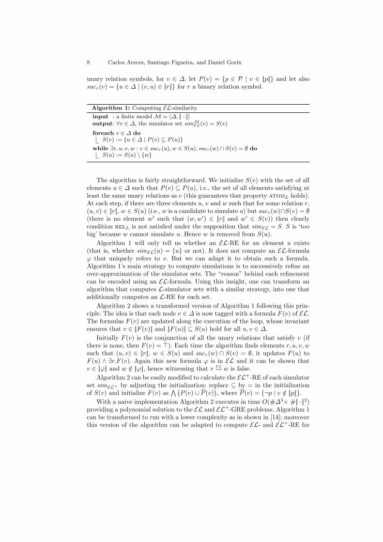
The algorithm is fairly straightforward. We initialize S(v) with the set of allelements u ∈ ∆ such that P (v) ⊆ P (u), i.e., the set of all elements satisfying atleast the same unary relations as v (this guarantees that property atomL holds).At each step, if there are three elements u, v and w such that for some relation r,(u, v) ∈ ||r||, w ∈ S(u) (i.e., w is a candidate to simulate u) but sucr(w)∩S(v) = ∅(there is no element w′ such that (w,w′) ∈ ||r|| and w′ ∈ S(v)) then clearlycondition relL is not satisfied under the supposition that simEL = S. S is ‘toobig’ because w cannot simulate u. Hence w is removed from S(u).

Algorithm 1 will only tell us whether an EL-RE for an element u exists(that is, whether simEL(u) = {u} or not). It does not compute an EL-formulaϕ that uniquely refers to v. But we can adapt it to obtain such a formula.Algorithm 1’s main strategy to compute simulations is to successively refine anover-approximation of the simulator sets. The “reason” behind each refinementcan be encoded using an EL-formula. Using this insight, one can transform analgorithm that computes L-simulator sets with a similar strategy, into one thatadditionally computes an L-RE for each set.

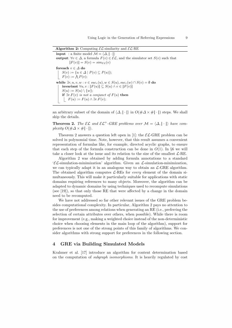
Algorithm 2 shows a transformed version of Algorithm 1 following this prin-ciple. The idea is that each node v ∈ ∆ is now tagged with a formula F (v) of EL.The formulas F (v) are updated along the execution of the loop, whose invariantensures that v ∈ ||F (v)|| and ||F (u)|| ⊆ S(u) hold for all u, v ∈ ∆.

Initially F (v) is the conjunction of all the unary relations that satisfy v (ifthere is none, then F (v) = >). Each time the algorithm finds elements r, u, v, wsuch that (u, v) ∈ ||r||, w ∈ S(u) and sucr(w) ∩ S(v) = ∅, it updates F (u) toF (u) ∧ ∃r.F (v). Again this new formula ϕ is in EL and it can be shown thatv ∈ ||ϕ|| and w /∈ ||ϕ||, hence witnessing that v

EL w is false.

Algorithm 2 can be easily modified to calculate the EL+-RE of each simulatorset simEL+ by adjusting the initialization: replace ⊆ by = in the initializationof S(v) and initialize F (v) as

∧(P (v) ∪ P (v)

), where P (v) = {¬p | v /∈ ||p||}.

With a naive implementation Algorithm 2 executes in time O(#∆3× #|| · ||2)providing a polynomial solution to the EL and EL+-GRE problems. Algorithm 1can be transformed to run with a lower complexity as in shown in [14]; moreoverthis version of the algorithm can be adapted to compute EL- and EL+-RE for


Algorithm 2: Computing EL-similarity and EL-RE

input : a finite model M = 〈∆, || · ||〉output: ∀v ∈ ∆, a formula F (v) ∈ EL, and the simulator set S(v) such that

||F (v)|| = S(v) = simEL(v)

foreach v ∈ ∆ doS(v) := {u ∈ ∆ | P (v) ⊆ P (u)};F (v) :=

∧P (v);

while ∃r, u, v, w : v ∈ sucr(u), w ∈ S(u), sucr(w) ∩ S(v) = ∅ doinvariant ∀u, v : ||F (u)|| ⊆ S(u) ∧ v ∈ ||F (v)||S(u) := S(u) \ {w};if ∃r.F (v) is not a conjunct of F (u) then

F (u) := F (u) ∧ ∃r.F (v);

an arbitrary subset of the domain of 〈∆, || · ||〉 in O(#∆×#|| · ||) steps. We shallskip the details.

Theorem 2. The EL and EL+-GRE problems over M = 〈∆, || · ||〉 have com-plexity O(#∆×#|| · ||).

Theorem 2 answers a question left open in [1]: the EL-GRE problem can besolved in polynomial time. Note, however, that this result assumes a convenientrepresentation of formulas like, for example, directed acyclic graphs, to ensurethat each step of the formula construction can be done in O(1). In §6 we willtake a closer look at the issue and its relation to the size of the smallest L-RE.

Algorithm 2 was obtained by adding formula annotations to a standard‘EL-simulation-minimization’ algorithm. Given an L-simulation-minimization,we can typically adapt it in an analogous way to obtain an L-GRE algorithm.The obtained algorithm computes L-REs for every element of the domain si-multaneously. This will make it particularly suitable for applications with staticdomains requiring references to many objects. Moreover, the algorithm can beadapted to dynamic domains by using techniques used to recompute simulations(see [19]), so that only those RE that were affected by a change in the domainneed to be recomputed.

We have not addressed so far other relevant issues of the GRE problem be-sides computational complexity. In particular, Algorithm 2 pays no attention tothe use of preferences among relations when generating an RE (i.e., preferring theselection of certain attributes over others, when possible). While there is roomfor improvement (e.g., making a weighted choice instead of the non-deterministicchoice when choosing elements in the main loop of the algorithm), support forpreferences is not one of the strong points of this family of algorithms. We con-sider algorithms with strong support for preferences in the following section.

4 GRE via Building Simulated Models

Krahmer et al. [17] introduce an algorithm for content determination basedon the computation of subgraph isomorphisms. It is heavily regulated by cost


functions and is therefore apt to implement different preferences. In fact, theyshow that using suitable cost functions it can simulate most of the previousproposals. Their algorithm takes as input a labeled directed graph G and a nodee and returns, if possible, a connected subgraph H of G, containing e and enoughedges to distinguish e from the other nodes.

In this section we will identify its underlying notion of expressiveness andwill extend it to accommodate other notions. To keep the terminology of [17],in what follows we may alternatively talk of labeled graphs instead of relationalmodels. The reader should observe that they are essentially the same mathe-matical object, but notice that in [17], propositions are encoded using loopingbinary relations (e.g., they write dog(e, e) instead of dog(e)).

The main ideas of their algorithm can be intuitively summarized as follows.Given two labeled graphs H and G, and vertices v of H and w of G, we say thatthe pair (v,H) refers to the pair (w,G) iff H is connected and H can be “placedover” G in such a way that: 1) v is placed over w; 2) each node of H is placed overa node of G with at least the same unary predicates (but perhaps more); and 3)each edge from H is placed over an edge with the same label. Furthermore, (v,H)uniquely refers to (w,G) if (v,H) refers to (w,G) and there is no vertex w′ 6= w inG such that (v,H) refers to (w′, G). The formal notion of a labeled graph being“placed over” another one is that of subgraph isomorphism: H = 〈∆H , || · ||H〉can be placed over G iff there is a labeled subgraph (i.e., a graph obtained fromG by possibly deleting certain nodes, edges, and propositions from some nodes)G′ = 〈∆G′ , || · ||G′〉 of G such that H is isomorphic to G′, which means that thereis a bijection f : ∆H → ∆G′ such that for all vertices u, v ∈ ∆H , u ∈ ||p||H ifff(u) ∈ ||p||G′ and (u, v) ∈ ||r||H iff (f(u), f(v)) ∈ ||r||G′ .

v

dog

v

dog

sniffs

dog

v

dogsmall

sniffsv

dog catsmall

sniffs

(i) (ii) (iii) (iv)

Fig. 2. Some connected subgraphs (v,H) of scene S in Figure 1.

As an example, consider the relational model depicted in Figure 1 as a labeledgraph G, and let us discuss the pairs of nodes and connected subgraphs (v,H)shown in Figure 2. Clearly, (i) refers to the pair (w,G) for any node w ∈ {a, b, d};(ii) refers to (w,G) for w ∈ {b, d}; and both (iii) and (iv) uniquely refer to (b,G).Notice that (i)–(iv) can be respectively realized as “a dog”, “a dog that sniffssomething”, “a small dog that sniffs a dog” (cf. γ1 in Table 1) and “the dog thatis sniffed by a small cat” (cf. γ4 in Table 1).

It is important to emphasize that there is a substantial difference betweenthe algorithm presented in [17] and the one we discussed in the previous sections:while the input is a labeled graph G and a target node v, the output is, in thiscase (and unlike the definition of L-GRE problem presented in §2 where theoutput is a formula), the cheapest (with respect to some, previously specified


cost function) connected subgraph H of G which uniquely refers to (v,G) if thereis such H, and ⊥ otherwise.

We will not deal with cost functions here; it is enough to know that a costfunction is a monotonic function that assigns to each subgraph of a scene grapha non-negative number which expresses the goodness of a subgraph –e.g. inFigure 2, one may tune the cost function so that (iii) is cheaper than (iv), andhence (iii) will be preferred over (iv).

For reasons of space we will not introduce here the detailed algorithm pro-posed in [17]. Roughly, it is a straightforward branch and bound algorithm thatsystematically tries all relevant subgraphs H of G by starting with the subgraphcontaining only vertex v and expanding it recursively by trying to add edgesfrom G that are adjacent to the subgraph H constructed up to that point. Inthe terminology of [17] a distractor is a node of G different from v that is alsoreferred by H. The algorithm ensures that a subgraph uniquely refers to thetarget v when it has no distractors. Reached this point we have a new candidatefor the solution, but there can be other cheaper solution so the search processcontinues until the cheapest solution is detected. Cost functions are used to guidethe search process and to give preference to some solutions over others.

Here is the key link between the graph-based method of [17] and our logical-oriented perspective: on finite relational models, subgraph isomorphism corre-sponds to FO−-simulations, in the sense that given two nodes u, v of G, there isa subgraph isomorphic to G via f , containing u and v, and such that f(u) = v iff

uFO−→ v. Having made explicit this notion of sameness and, with it, the logical

language associated to it, we can proceed to generalize the algorithm to make itwork for other languages, and to adapt it in order to output a formula insteadof a graph. This is shown in Algorithms 3 and 4.

Algorithm 3: makeREL(v)

input : an implicit finiteG = 〈∆G, || · ||〉 andv ∈ ∆G

output: an L-RE for v in G ifthere is one, or else ⊥

H := 〈{v}, ∅〉;f := {v 7→ v};H ′ := findL (v,⊥, H, f);

return buildFL (H ′, v);

Algorithm 4: findL(v, best , H, f)

if best 6= ⊥ ∧ cost(best) ≤ cost(H) thenreturn best

distractors := {n | n ∈ ∆G, n 6= v, vL→n};

if distractors = ∅ thenreturn H

foreach 〈H ′, f ′〉 ∈ extendL(H, f) doI := findL (v, best , H ′, f ′);if best = ⊥∨ cost(I) ≤ cost(best) then

best := I

return best ;

These algorithms are parametric on L; to make them concrete, one needs toprovide appropriate versions of buildFL and extendL. The former transformsthe computed graph which uniquely refers to the target v into an L-RE formulafor v; the latter tells us how to extend H at each step of the main loop ofAlgorithm 4. Note that, unlike the presentation of [17], makeREL computes notonly a graph H but also an L-simulation f . In order to make the discussion


of the differences with the original algorithm simpler, we analyze next the caseL = FO− and L = EL.

The case of FO−. From the computed cheapest isomorphic subgraph H ′ one caneasily build an FO−-formula that uniquely describes the target v, as is shown inAlgorithm 5. Observe that if FO-simulations were used instead, we would haveto include also which unary and binary relations do not hold in H ′.

Algorithm 5: buildFFO−(H ′, v)

let H ′ = 〈{a1 . . . an}, || · ||〉,v = a1;

γ :=∧

ai 6=aj

(xi 6≈ xj) ∧∧

(ai,aj)∈||r||

r(xi, xj) ∧∧

ai∈||p||

p(xi)

return ∃x2 . . .∃xn.γ;

Algorithm 6: extendFO−(H, f)

A := {H+p(u) | u ∈ ∆H ,u ∈ ||p||G \ ||p||H};

B := {H+r(u, v) | u ∈ ∆H ,{(u, v), (v, u)} ∩ ||r||G \ ||r||H 6= ∅};return (A ∪B)× {id};

Regarding the function which extends the given graph in all possible ways (Algo-rithm 6), since H is a subgraph of G, f is the trivial identity function id(x ) = x.We will see the need for f when discussing the case of less expressive logicslike EL. In extendFO− we follow the notation of [17] and write, for a relationalmodel G = 〈∆, || · ||〉, G + p(u) to denote the model 〈∆ ∪ {u}, || · ||′〉 such that||p||′ = ||p|| ∪ {u} and ||q||′ = ||q|| when q 6= p. Similarly, G + r(u, v) denotes themodel 〈∆∪{u, v}, || · ||′〉 such that ||r||′ = ||r||∪{(u, v)} and ||q||′ = ||q|| when q 6= r.It is clear, then, that this function is returning all the extensions of H by addinga missing attribute or relation to H, just like is done in the original algorithm.

The case of EL. Observe that findEL uses an EL-simulation, and any FO−-simulation is an EL-simulation. One could, in principle, just use extendFO− alsofor EL. If we do this, the result of findEL will be a subgraph H of G such thatfor every EL-simulation ∼, u ∼ v iff u = v. The problem is that this subgraphH may contain cycles and, as it is well known, EL (even ALC) are incapable todistinguish a cycle from its unraveling9. Hence, although subgraph isomorphismget along with FO−, it is too strong to deal with EL.

A well-known result establishes that every relational modelM is equivalent,with respect to EL-formulas,10 to the unraveling of M. That is, any model andits unraveling satisfy exactly the same EL-formulas. Moreover, the unravelingof M is always a tree, and as we show in Algorithm 7, it is straightforward toextract a suitable EL-formula from a tree.

Therefore, we need extendEL to return all the possible “extensions” of H.Now “extension” does not mean to be a subgraph of the original graph G any-more. We do this by either adding a new proposition or a new edge that ispresent in the unraveling of G but not in H. This is shown in Algorithm 8.

9 Informally, the unraveling of G, is a new graph, whose points are paths of G from agiven starting node. That is, transition sequences in G are explicitly represented asnodes in the unraveled model. See [3] for a formal definition.

10 Actually, the result holds even for ALC-formulas.


Algorithm 7: buildFEL(H ′, v)

requires H ′ to be a treeγ := {∃r.buildFEL(H ′, u) |

(v, u) ∈ ||r||};return (

∧γ) ∧ (

∧v∈||p|| p);

Algorithm 8: extendEL(H, f)

A :={〈H+p(u), f〉 | u ∈ ∆H , u ∈ ||p||G \ ||p||H};

B := ∅;foreach u ∈ ∆G do

foreach uH ∈ ∆H/(f(uh), u) ∈ ||r||G doif ∀v : (uH , v) ∈ ||r||H ⇒ f(v) 6= uthen

n := new node;B := B ∪{〈H + r(uH , n), f ∪ {n 7→ u}〉};

return A ∪B;

Observe that the behavior of findEL is quite sensible to the cost function em-ployed. For instance, on cyclic models, a cost function that does not guaranteethe unraveling is explored in a breadth-first way may lead to non-termination(since findEL may loop exploring an infinite branch).

As a final note on complexity, although the set of EL-distractors may becomputed more efficiently than FO−-distractors (since EL-distractors can becomputed in polynomial time, and computing FO−-distractors seems to requirea solution to the subgraph isomorphism problem which NP-complete), we cannotconclude that findEL is more efficient than findFO− in general: the model builtin the first case may be exponentially larger –it is an unraveling, after all. Wewill come back to this in §6.

5 Combining GRE Methods

An appealing feature of formulating the GRE problem modulo expressivity isthat one can devise general strategies that combine L-GRE algorithms. We il-lustrate this with an example.

The algorithms based on L-simulator sets like the ones in §3 simultaneouslycompute referring expressions for every object in the domain, and do this formany logics in polynomial time. This is an interesting property when one antic-ipates the need of referring to a large number of elements. However, this familyof algorithms is not as flexible in terms of implementing preferences as those weintroduced in §4 –though some flexibility can be obtained by using cost func-tions for selecting u, v and w in the main loop of Algorithm 2 instead of thenon-deterministic choices.

There is a simple way to obtain an algorithm that is a compromise betweenthese two techniques. Let A1 and A2 be two procedures that solve the L-GREproblem based on the techniques of §3 and §4, respectively. One can first com-pute an L-RE for every possible object using A1 and then (lazily) replace thecalculated RE for u with A2(u) whenever the former does not conform to somepredefined criterion. This is correct but we do better, taking advantage of theequivalence classes obtained using A1.


Since A1 computes, for a givenM = 〈∆, || · ||〉, the set sim(u) for every u ∈ ∆,one can build in polynomial time, using the output of A1, the model ML =〈{[u] | u ∈ ∆}, || · ||L〉, such that: [u] = {v | u L→ v and v

L→ u} and ||r||L ={([u1] . . . [un]) | (u1 . . . un) ∈ ||r||}. ML is known as the L-minimization of M.By a straightforward induction on γ one can verify that (u1 . . . un) ∈ ||γ|| iff([u1] . . . [un]) ∈ ||γ||L and this implies that γ is an L-RE for u in M iff it is anL-RE for [u] in ML.

If M has a large number of indistinguishable elements (using L), then MLwill be much smaller thanM. Since the computational complexity of A2 dependson the size of M, for very large scenes, one should compute A2([u]) instead.

6 On the Size of Referring Expressions

The expressive power of a language L determines if there is an L-RE for anelement u. It also influences the size of the shortest L-RE (when they exist).Intuitively, with more expressive power we are able to ‘see’ more differences andtherefore have more resources at hand to build a shorter formula.

A natural question is, then, whether we can characterize the relative size ofthe L-REs for a given L. That is, if we can give (tight) upper bounds for the sizeof the shortest L-REs for the elements of an arbitrary model M, as a functionof the size of M.

For the case of one of the most expressive logics considered in this article,FO−, the answer follows from algorithm makeREFO− in §4. Indeed, if an FO−-RE exists, it is computed by buildFFO− from a model H that is not bigger thanthe input model. It is easy to see that this formula is linear in the size of H and,therefore the size of any FO−-RE is O(#∆+ #|| · ||). It is not hard to see thatthis upper bound holds for FO-REs too.

One is tempted to conclude from Theorem 2 that the size of the shortest EL-RE is O(#∆ ×#|| · ||), but there is a pitfall. Theorem 2 assumes that formulasare represented as a DAG and it guarantees that this DAG is polynomial inthe size of the input model. One can easily reconstruct (the syntax tree of) theformula from the DAG, but this, in principle, may lead to a exponential blow-up –the result will be an exponentially larger formula, but composed of only apolynomial number of different subformulas. As the following example shows,it is indeed possible to obtain an EL-formula that is exponentially larger whenexpanding the DAG representation generated by Algorithm 2.

Example 1. Consider a language with only one binary relation r, and let M =〈∆, || · ||〉 where ∆ = {1, 2, . . . , n} and (i, j) ∈ ||r|| iff i < j. Algorithm 2 initializesF (j) = > for all j ∈ ∆. Suppose the following choices in the execution: Fori = 1, . . . , n − 1, iterate n − i times picking v = w = n − i + 1 and successivelyu = n − i, . . . , 1. It can be shown that each time a formula F (j) is updated, itchanges from ϕ to ϕ ∧ ∃r.ϕ and hence it doubles its size. Since F (1) is updatedn− 1 many times, the size of F (1) is greater than 2n.


The large EL-RE of Example 1 is due to an unfortunate (non-deterministic)choice of elements. Example 2 shows that another execution leads to a quadraticRE (but notice the shortest one is linear: (∃r)(n−1).>).

Example 2. Suppose now that in the first n−1 iterations we successively choosev = w = n − i and u = v − 1 for i = 0 . . . n − 2. It can be seen that for furtherconvenient choices, F (1) is of size O(n2).

But is it always possible to obtain an EL-RE of size polynomial in the sizeof the input model, when we represent a formula as a string, and not as a DAG?In [12] it is shown that the answer is ‘no’: for L ∈ {ALC, EL, EL+}, the lowerbound for the length of the L-RE is exponential in the size of the input model11,and this lower bound is tight.

7 Conclusions

The content determination phase during the generation of referring expressionsidentifies which ‘properties’ will be used to refer to a given target object or setof objects. What is considered as a ‘property’ is specified in different ways byeach of the many algorithms for content determination existing in the literature.In this article, we put forward that this issue can be addressed by decidingwhen two elements should be considered to be equal, that is, by deciding whichdiscriminatory power we want to use. Formally, the discriminatory power wewant to use in a particular case can be specified syntactically by choosing aparticular formal language, or semantically, by choosing a suitable notion ofsimulation. It is irrelevant whether we choose first the language (and obtain theassociated notion of simulation afterwards) or vice versa.

We maintain that having both at hand is extremely useful. Obviously, theformal language will come handy as representation language for the output tothe content determination problem. But perhaps more importantly, once wehave fixed the expressivity we want to use, we can rely on model theoreticalresults defining the adequate notion of sameness underlying each language, whichindicates what can and cannot be said (as we discussed in §2). Moreover, we cantransfer general results from the well-developed fields of computational logics andgraph theory as we discuss in §3 and §4, where we generalized known algorithmsinto families of GRE algorithms for different logical languages.

An explicit notion of expressiveness also provides a cleaner interface, eitherbetween the content determination and surface realization modules or betweentwo collaborating content determination modules. An instance of the latter wasexhibited in §5.

As a future line of research, one may want to avoid sticking to a fixed L butinstead favor an incremental approach in which features of a more expressivelanguage L1 are used only when L0 is not enough to distinguish certain element.

11 More precisely, there are infinite models G1, G2, . . . such that for every i, the size ofGi is linear in i but the size of the minimum RE for some element in Gi is boundedfrom below by a function which is exponential on i.


References

1. Areces, C., Koller, A., Striegnitz, K.: Referring expressions as formulas of descrip-tion logic. In: Proc. of the 5th INLG. Salt Fork, OH, USA (2008)

2. Baader, F., McGuiness, D., Nardi, D., Patel-Schneider, P. (eds.): The DescriptionLogic Handbook: Theory, implementation and applications. Cambridge UniversityPress (2003)

3. Blackburn, P., de Rijke, M., Venema, Y.: Modal Logic. Cambridge University Press(2001)

4. Dale, R.: Cooking up referring expressions. In: Proc. of the 27th ACL (1989)5. Dale, R., Haddock, N.: Generating referring expressions involving relations. In:

Proc. of the 5th EACL (1991)6. Dale, R., Reiter, E.: Computational interpretations of the Gricean maxims in the

generation of referring expressions. Cognitive Science 19 (1995)7. Dale, R., Viethen, J.: Referring expression generation through attribute-based

heuristics. In: Proc. of the 12th ENLG workshop. pp. 58–65 (2009)8. van Deemter, K.: Generating referring expressions: Boolean extensions of the in-

cremental algorithm. Computational Linguistics 28(1), 37–52 (2002)9. van Deemter, K., van der Sluis, I., Gatt, A.: Building a semantically transparent

corpus for the generation of referring expressions. In: Proc. of the 4th INLG (2006)10. Dovier, A., Piazza, C., Policriti, A.: An efficient algorithm for computing bisimu-

lation equivalence. Theor. Comput. Sci 311, 221–256 (2004)11. Ebbinghaus, H., Flum, J., Thomas, W.: Mathematical Logic. Springer (1996)12. Figueira, S., Gorın., D.: On the size of shortest modal descriptions. In: Advances

in Modal Logic. vol. 8, pp. 114–132 (2010)13. Garey, M., Johnson, D.: Computers and Intractability: A Guide to the Theory of

NP-Completeness. W. Freeman (1979)14. Henzinger, M.R., Henzinger, T.A., Kopke, P.W.: Computing simulations on finite

and infinite graphs. In: Proc. of 36th Annual Symposium on Foundations of Com-puter Science. pp. 453–462. IEEE Computer Society Press (1995)

15. Hopcroft, J.: An nlog(n) algorithm for minimizing states in a finite automaton. InZ. Kohave, editor, Theory of Machines and Computations, Academic Press (1971)

16. Horacek, H.: An algorithm for generating referential descriptions with flexible in-terfaces. In: Proc. of the 35th ACL. pp. 206–213 (1997)

17. Krahmer, E., van Erk, S., Verleg, A.: Graph-based generation of referring expres-sions. Computational Linguistics 29(1) (2003)

18. Paige, R., Tarjan, R.: Three partition refinement algorithms. SIAM J. Comput.16(6), 973–989 (1987)

19. Saha, D.: An incremental bisimulation algorithm. In: Arvind, V., Prasad, S. (eds.)FSTTCS 2007: Foundations of Software Technology and Theoretical ComputerScience, LNCS, vol. 4855, pp. 204–215. Springer Berlin / Heidelberg (2007)

20. Stone, M.: On identifying sets. In: Proc. of the 1st INLG (2000)21. Stone, M., Webber, B.: Textual economy through close coupling of syntax and

semantics. In: Proc. of the 9th INLG workshop. pp. 178–187 (1998)22. Viethen, J., Dale, R.: Algorithms for generating referring expressions: Do they do

what people do? In: Proc. of the 4th INLG (2006)

Using Logic in the Generation of Referring Expressions · Using Logic in the Generation of...

Documents

Transcript of Using Logic in the Generation of Referring Expressions · Using Logic in the Generation of...