Using Implied Volatility to Measure Uncertainty About ... · PDF fileFEDERAL RESERVE BANK OF...

FEDERAL RESERVE BANK OF ST. LOUIS REVIEW MAY/JUNE 2005 407

Using Implied Volatility to Measure UncertaintyAbout Interest Rates

Christopher J. Neely

biased predictor of volatility, which often encom-passes other forecasts.

Readers who are already familiar with thebasics of options might wish to skip the first sec-tion of this article; it explains how option pricesare determined by the cost of a portfolio of assetsthat can be dynamically traded to provide theoption payoff. Readers who are unfamiliar withoptions might wish to start with the glossary ofoption terms at the end of this article and the inserton the basics of options (boxed insert 1). The sec-ond section reviews the relation between IV andfuture volatility, showing how option pricingformulas can be “inverted” to estimate volatility.The third section measures the IV of short-terminterest rates over time and discusses how suchmeasures can aid in interpreting economic events.

HOW DOES ONE PRICEOPTIONS?

Options are a derivative asset. That is, optionpayoffs depend on the price of the underlyingasset. Because of this, one can often exactlyreplicate the payoff to an option with a suitably

E conomists often use asset prices alongwith models of their determination toderive financial markets’ expectationsof events. For example, monetary econ-

omists use federal funds futures prices to meas-ure expectations of interest rates (Krueger andKuttner, 1995; Pakko and Wheelock, 1996).Similarly, a large literature on fixed and targetzone exchange rates has used forward exchangerates to measure the credibility of exchange rateregimes or to predict their collapse (Svensson,1991; Rose and Svensson, 1991, 1993; Neely,1994).

But it is often helpful to gauge the uncertaintyassociated with future asset prices as well as theirexpectation. Because option prices depend onthe perceived volatility of the underlying asset,they can be used to quantify the expected volatil-ity of an asset price (Latane and Rendleman, 1976).Such estimates of volatility, called implied volatil-ity (IV), require some heroic assumptions aboutthe stochastic (random) process governing theunderlying asset price. But the usual assumptionsseem to provide very reasonable forecasts ofvolatility. That is, IV is a highly significant but

Option prices can be used to infer the level of uncertainty about future asset prices. The first twoparts of this article explain such measures (implied volatility) and how they can differ from themarket’s true expectation of uncertainty. The third then estimates the implied volatility of three-month eurodollar interest rates from 1985 to 2001 and evaluates its ability to predict realizedvolatility. Implied volatility shows that uncertainty about short-term interest rates has been fallingfor almost 20 years, as the levels of interest rates and inflation have fallen. And changes in impliedvolatility are usually coincident with major news about the stock market, the real economy, andmonetary policy.

Federal Reserve Bank of St. Louis Review, May/June 2005, 87(3), pp. 407-25.

Christopher J. Neely is a research officer at the Federal Reserve Bank of St. Louis. Joshua Ulrich provided research assistance.

© 2005, The Federal Reserve Bank of St. Louis.

Neely

408 MAY/JUNE 2005 FEDERAL RESERVE BANK OF ST. LOUIS REVIEW

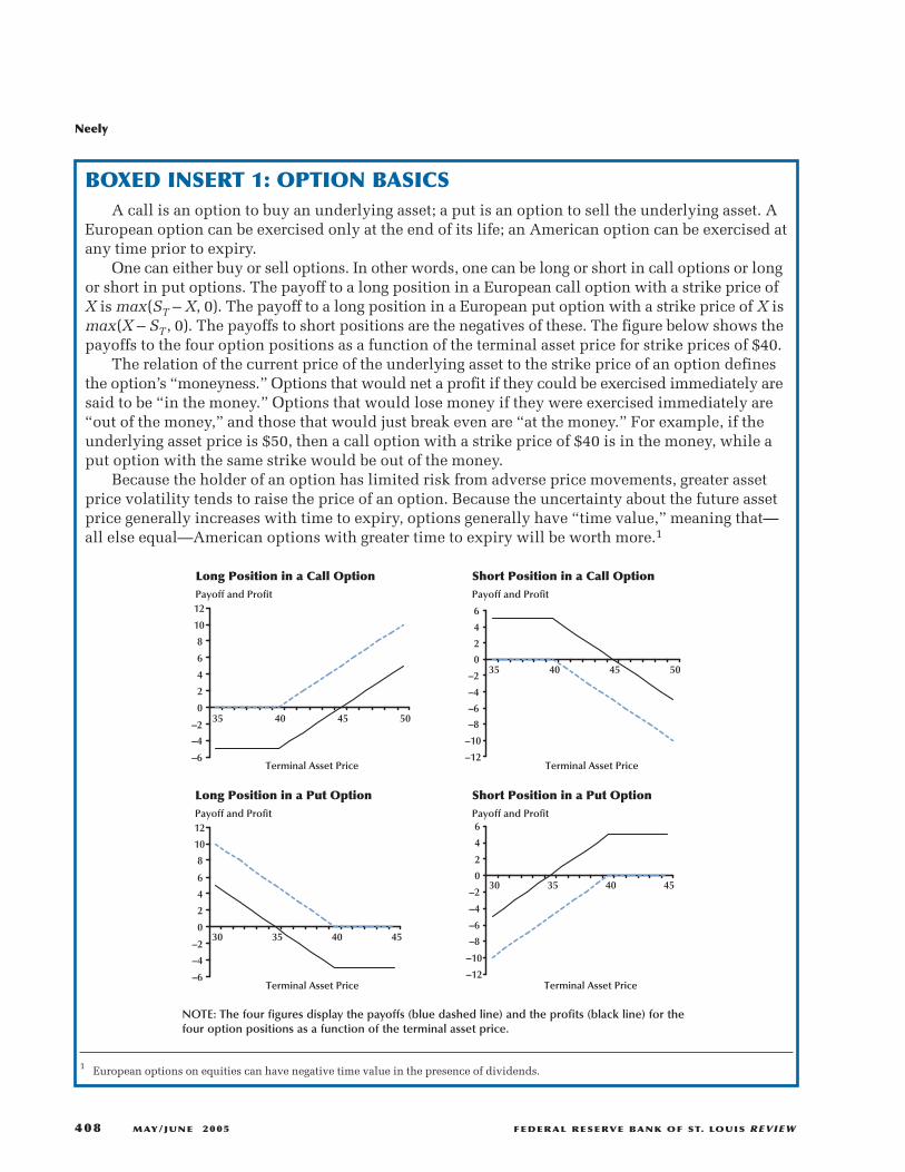
BOXED INSERT 1: OPTION BASICSA call is an option to buy an underlying asset; a put is an option to sell the underlying asset. A

European option can be exercised only at the end of its life; an American option can be exercised atany time prior to expiry.

One can either buy or sell options. In other words, one can be long or short in call options or longor short in put options. The payoff to a long position in a European call option with a strike price ofX is max(ST – X, 0). The payoff to a long position in a European put option with a strike price of X ismax(X – ST, 0). The payoffs to short positions are the negatives of these. The figure below shows thepayoffs to the four option positions as a function of the terminal asset price for strike prices of $40.

The relation of the current price of the underlying asset to the strike price of an option definesthe option’s “moneyness.” Options that would net a profit if they could be exercised immediately aresaid to be “in the money.” Options that would lose money if they were exercised immediately are“out of the money,” and those that would just break even are “at the money.” For example, if theunderlying asset price is $50, then a call option with a strike price of $40 is in the money, while aput option with the same strike would be out of the money.

Because the holder of an option has limited risk from adverse price movements, greater assetprice volatility tends to raise the price of an option. Because the uncertainty about the future assetprice generally increases with time to expiry, options generally have “time value,” meaning that—all else equal—American options with greater time to expiry will be worth more.1

1 European options on equities can have negative time value in the presence of dividends.

–6

–4

–2

0

2

4

6

8

10

12

35 40 45 50

Terminal Asset Price–12

–10

–8

–6

–4

–2

0

2

4

6

35 40 45 50

Terminal Asset Price

–6

–4

–2

0

2

4

6

8

10

12

30 35 40 45

Terminal Asset Price–12

–10

–8

–6

–4

–2

0

2

4

6

30 35 40 45

Terminal Asset Price

Payoff and ProfitPayoff and Profit

Payoff and Profit Payoff and Profit

Long Position in a Call Option Short Position in a Call Option

Long Position in a Put Option Short Position in a Put Option

NOTE: The four figures display the payoffs (blue dashed line) and the profits (black line) for thefour option positions as a function of the terminal asset price.

managed portfolio of the underlying asset and ariskless asset. The set of assets that replicates theoption payoff is called the replicating portfolio.This section explains how arbitrage equalizes theprice of the option and the price of the replicatingportfolio.

Pricing an Option with a Binomial Tree

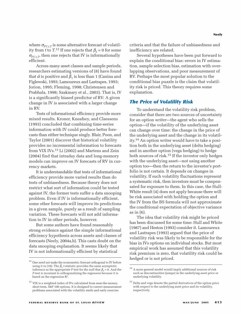
A simple numerical example will help explainhow the price of an option is equal to the price ofa portfolio of assets that can replicate the optionpayoff. Suppose that a stock price is currently $10and that it will either be $12 or $8 in one year.1

Suppose further that interest rates are currently5 percent. A one-year European call option witha strike price of $10 gives the buyer the right, butnot the obligation, to purchase the stock for $10at the end of one year.2 If the stock price goes upto $12, the option will be worth $2 because it con-fers the right to pay $10 for an asset with a $12market price. But if the stock price falls to $8, theoption will be worthless because no one wouldwant to buy a stock at the strike price when themarket price is lower.

Suppose that the First Bank of Des Peres(FBDP) sells one call option on one share of a non-dividend-paying stock and simultaneously buyssome amount, call it ∆, shares of the stock. If thestock price goes up to $12, the FBDP’s portfoliowill be worth the value of its stock, less the valueof the option: $12∆ – $2. If the stock price falls to$8, the option will be worthless and the FBDP’sportfolio will only be worth $8∆. The key to optionpricing is that the FBDP can choose ∆ to make thevalue of its portfolio the same in either state ofthe world: It chooses ∆ = 1/2, to make $12∆ – $2 =$8∆ – $0. That is, if the FBDP buys ∆ = 1/2 unitsof the stock after selling the call option, it willhave a riskless payoff to its portfolio of $4.

Because this payoff is riskless, the portfolioof a short call option and 1/2 share of the stock

must earn the riskless return. If it did not, therewould be an arbitrage opportunity. The initialcost of the portfolio is the cost of the ∆ shares ofstock ($10∆) less the price of the call option ($C).The initial cost of the portfolio must equal itsdiscounted riskless payoff ($4e–0.05):

(1) .3

Using the fact that ∆ = 1/2, the price of the calloption must be

(2) .

If the price of the call option were more than$1.1951, one could make a riskless profit by sell-ing the option and holding 1/2 shares of the stock.4

If the call option price were less than $1.1951, onecould make an arbitrage profit by buying the calland shorting 1/2 shares of the stock.

An equivalent way to look at the problem isto create the portfolio that replicates the initialinvestment/payoff of the call option. That is, theFBDP could borrow $5 and buy 1/2 of a share ofthe stock. At the end of the year, the 1/2 share ofstock would be worth either $6 or $4 and theFBDP would owe ($5e0.05=) $5.2564 on the moneyit borrowed. The initial investment would be zeroand the payoff would be $0.7436 in the first stateand –$1.2564 in the second state. This is the sameinitial investment/payoff structure as borrowing$1.1951 and buying the call option with a strikeprice of $10. In other words, the portfolio thatreplicates the call option in this example is a 1/2

share of the stock and an equal short position ina riskless bond.

Introductory textbooks on derivatives, likeHull (2002), Jarrow and Turnbull (2000), orDubofsky and Miller (2003), provide a much more

C e= − =−$ $ $ ..1012

4 1 19510 05

$ $ .10 4 0 05∆ − = −C e

Neely


1 This example assumes that the stock pays no dividends. If it didpay known dividends, it could be priced in a similar way.

2 A European option confers the right to buy or sell the underlyingasset for a given price at the expiry of the option. An Americanoption can be exercised on or before the expiry date. A call (put)option confers the right, but not the obligation, to buy (sell) a par-ticular asset at a given price, called the strike price.

3 If the continuously compounded interest rate is 5 percent, theprice of a riskless bond with a one-year payoff of $4 would have aprice of $4e–0.05.

4 Suppose that the call option cost $1.30. One would sell the calloption, borrow $3.70, and use the proceeds of the option sale andthe borrowed funds to buy 1/2 share of stock. If the first state of theworld occurs, the writer of the option will have $6 in stock but willpay $2 to the option buyer and (3.70e0.05 =) $3.89 to the bank thatloaned him the funds originally. He will make a riskless profit of$0.11. Similarly, in the second state of the world, the option expiresworthless and the option writer sells the 1/2 share of stock for $4,pays the loan off with $3.89 and again makes $0.11 riskless profit.

extensive treatment of binomial trees as well asinformation about how options pricing formulaschange for different types of assets.

Black-Scholes Valuation

The preceding example, illustrated in Figure 1,was a one-step binomial tree. The option pricewas calculated under the assumption that thestock could take one of two known values atexpiry. Suppose instead that the stock could moveup or down several times before expiration. Inthis case, one can calculate an option price bycomputing each possible value of the option atexpiry and working backward to get the price atthe beginning of the tree. As the asset prices riseand the call option goes “into the money,” thereplicating portfolio holds more of the underlyingasset and less of the riskless bond.5 At each pointin time, the option writer chooses the position inthe underlying asset to maintain a riskless payoffto the hedged portfolio—the combination of thepositions in the option, the underlying asset, andthe riskless bond. The position in the underlyingasset is equal to the rate of change in the optionvalue with respect to the underlying asset price.

This rate of change is known as the option’s“delta” and the continuous process of adjustmentof the underlying asset position is known as “deltahedging.” The limit of the formula for an optionprice from an n-step binomial tree, as n goes toinfinity, is the Black-Scholes (BS) formula (Blackand Scholes, 1972).6

The BS formula expresses the value of aEuropean call or put option as a function of theunderlying asset price (S), the strike price (X), theinterest rate (r), time to expiry (T), and the varianceof the underlying asset return (σ2). Higher assetprice volatility means higher option prices becausethe downside risk is always limited, whereas theupside potential is not. Therefore, option pricesincrease with expected volatility. The formula forthe price of a European call option on a spot assetthat pays no dividends or interest is the following:

(3) ,

where and

and N (*) is the cumulative normal density func-tion. Hull (2002), Jarrow and Turnbull (2000), andDubofsky and Miller (2003) provide formulas forput options and options on other types of assets.

The BS formula strictly applies to Europeanoptions only—not to American options, whichcan be exercised any time prior to expiry—and itrequires modifications for assets that pay divi-dends, such as stocks, or that don’t require aninitial outlay, such as futures.7 Further, the BSmodel makes some strong assumptions: that theunderlying asset price follows a lognormal randomwalk, that the riskless rate is a known functionof time, that one can continuously adjust one’s

dS X r T

Td T2

02

1

2=

+ −= −

ln( / ) ( / )σσ

σ

dS X r T

T10

2 2=

+ +ln( / ) ( / )σσ

C S N d Xe N drT= − −0 1 2( ) ( )

Neely


Figure 1

Pricing a Call Option with a Binomial Tree

NOTE: The figure illustrates values that a hypothetical stockcould take, along with the value of a call option on that stockwith a strike price of $10.

Stock Price = $12Option Value = $2

Stock Price = $8Option Value = $0

Stock Price = $10Option Price = ?

5 A call (put) option is said to be “in the money” if the underlyingasset price is greater (less) than the strike price. If the underlyingasset price is less (greater) than the strike price, the call (put) optionis “out of the money.” When the underlying asset price is near (at)the strike price, the option is “near (at) the money.”

6 There are several ways to derive the BS formula that differ in theirrequired assumptions (Merton, 1973b). Wilmott, Howison, andDewynne (1995) provide a nice introduction to the mathematicsof the BS formula and Wilmott (2000) extends that treatment tocover the price of volatility risk. Boyle and Boyle (2001) discussthe history of option pricing formulas.

7 Black (1976) provides the formula for options on futures, ratherthan spot assets. Barone-Adesi and Whaley (1987) provide anapproximation to the BS formula that accounts for early exercise.

position in the underlying asset (delta hedging),and that there are no transactions costs on theunderlying asset and no arbitrage opportunities.Despite these strong assumptions, the BS model isvery widely used by practitioners and academics,often fitting the data reasonably well even whenits assumptions are clearly violated.

Does IV Predict Realized Volatility?

The BS model expresses the price of aEuropean call or put option (C or P) as a functionof five arguments {S, X, r, T, and σ2}. Of those sixquantities, five are observable as market prices orfeatures of the option contract {C, S, X, r, T}. TheBS formula is frequently inverted to solve for thesixth quantity, the IV {σ} of log asset returns interms of the observed quantities. This IV is used topredict the volatility of the asset return to expiry.

Ironically, the BS formula usually used toderive IV assumes that volatility is constant. Hulland White (1987) provide the foundation for thepractice of using a constant-volatility model topredict stochastic volatility (SV): If volatilityevolves independently of the underlying assetprice and no priced risk is associated with theoption, the correct price of a European optionequals the expectation of the BS formula, evalu-ating the variance argument at average varianceuntil expiry:

(4) ,

where the average variance until expiry isdenoted as

and its square root is usually referred to as realizedvolatility (RV).8

Bates (1996) points out that the expectationin (4) is taken with respect to variance until expiry,not standard deviation until expiry. Therefore,one cannot use the linearity of the BS formulawith respect to standard deviation to justify pass-

VT t

V dt TT

, =− ∫1

ττ τ

C S V t C V h V dV

E C V V

t tBS

tT

t

BSt T t

( , , ) ( ) ( )

[ ( ),

= ∫

=

σ 2

]]

ing the expectation through the BS formula. Thatis, one cannot claim that the correct price of a calloption under stochastic volatility is the BS priceevaluated at the expected value of the standarddeviation until expiry. That is, it is not true that

(5) .

Instead, Bates (1996) approximates the relationbetween the BS IV and expected variance untilexpiry with a Taylor series expansion of the BSprice for an at-the-money option. That is, for at-the-money options, the BS formula for futuresreduces to

.

This can be approximated with a second-orderTaylor expansion of N(*) around zero, whichyields

.

Another second-order Taylor expansion of thatapproximation around the expected value ofvariance until expiry shows that the BS IV isapproximately the expected variance until expiry:

(6) .

That is, the BS-implied variance (σBS2 ) understates

the expected variance of the asset until expiry(EtV

–t,T). Similarly, BS-implied standard deviation

(σBS) slightly understates the expected standarddeviation of asset returns.9

The Volatility Smile

Volatility is constant in the BS model; IV doesnot vary with the “moneyness” of the option.That is, if the BS model assumptions were literallytrue, the IV from a deep-in-the-money call shouldbe the same as that from an at-the-money call oran in-the-money put. In reality, for most assets, IVdoes vary with moneyness. A graph of IV versusmoneyness is often referred to as the “volatility

ˆ( )

( ),

,,σBS

t T

t t Tt t T

Var V

E VE V2

2

2

118

≈ −

C e F TBS rT≈ − σ π/ ( )2

C e F N TBS rT=

−

− 2

12

1σ

C S V t C E V Vt tBS

t T t, , ,( ) = ( )

Neely


8 Romano and Touzi (1997) extend the Hull and White (1987) resultto include models that permit arbitrary correlation between returnsand volatility, like the Heston (1993) model.

9 Note that (6) depends on (4), which assumes that there is no pricedrisk associated with holding the option. That is, (6) requires thatchanges in volatility do not create priced risk for an option writer.

smile” or “volatility smirk,” depending on theshape of the relation. Research attributes thevolatility smile to deviations from the BS assump-tions about the evolution of the underlying assetprices, such as the presence of stochastic volatility,jumps in the price of the underlying asset, andjumps in volatility (Bates, 1996, 2003).

The existence of the volatility smile brings upthe question of which strike prices—or combina-tions of strike prices—to use to compute IV. Inpractice, IV is usually computed from a few near-the-money options for three reasons (Bates, 1996):(i) The BS formula is most sensitive to IV for at-the-money options. (ii) Near-the-money optionsare usually the most heavily traded, resulting insmaller pricing errors. (iii) Beckers (1981) showedthat IV from at-the-money options provides thebest estimates of future realized volatility. Whileresearchers have varied the number and types ofoptions as well as the weighting procedure, it hasbeen common to rely heavily on a few at-the-money options.

Constructing IV from Options Data

At each date, IV is chosen to minimize theunweighted sum of squared deviations of Barone-Adesi and Whaley’s (1987) formula for pricingAmerican options on futures with the actual settle-ment prices for the two nearest-to-the-money calloptions and two nearest-to-the-money put optionsfor the appropriate futures contract.10 That is, IVis computed as follows:

(7) ,

where Pri,t is the observed settlement premium(price) of the ith option on day t and BAWi (*) isthe appropriate call or put formula as a functionof the IV.

Before being used in the minimization of (7),the data were checked to make sure that theyobeyed the inequality restrictions implied by theno-arbitrage conditions on American optionsprices: C $ F – X and P $ X – F, where F is the

σ σσIV t T ii

t T i tt TBAW Pr, , , ,argmin ( ( ) )

,= ∑ −

=1

42

price of the underlying futures contract. Theseconditions apply because an American option—which can be exercised at any time—must alwaysbe worth at least its value if exercised immediately.Options prices that did not obey these relationswere discarded. In addition, the observation wasdiscarded if there was not at least one call andone put price.

THE PROPERTIES OF IMPLIEDVOLATILITYHow Well Does IV Predict RV?

Equation (6) says that BS IV is approximatelythe conditional expectation of RV(V

–t,T). This

relation has two testable implications: IV shouldbe an unbiased predictor of RV; no other forecastshould improve the forecast from IV. If IV is anunbiased predictor of RV, one should find that{α, β1} = {0, 1} in the following regression:

(8) ,

where σRV,t,T denotes the RV of the asset returnfrom time t to T and σIV,t,T is IV at t for an optionexpiring at T.11 RV is the annualized standarddeviation of asset returns from t to T:

(9) ,

where Ft is the asset price at t and there are 250business days in the year.

The other commonly investigated hypothesisabout IV is that no other forecast improves its fore-casts of RV. If IV does subsume other informationin this way, it is said to be an “informationallyefficient predictor” of volatility. Researchersinvestigate this issue with variants of the followingencompassing regression:

(10) ,σ α β σ β σ εRV t T IV t T FV t T t, , , , , ,= + + +1 2

σRV t T t T i ii t

TV

T tF F, , , ln( / )= =

−∑ −=

2501

σ α β σ εRV t T IV t T t, , , ,= + +1

Neely


10 The results in this paper are almost indistinguishable when donewith European option pricing formulas (Black, 1976) or the Barone-Adesi and Whaley correction for American options.

11 Researchers also estimate (8) with realized and implicit variances,rather than standard deviations. The results from such estimationsprovide similar inference to those done with variances. Otherauthors argue that because volatility is significantly skewed, oneshould estimate (8) with log volatility. Equation (6) shows thatuse of logs introduces another source of bias into the theoreticalrelation between RV and IV.

where σFV,t,T is some alternative forecast of volatil-ity from t to T.12 If one rejects that β2 = 0 for someσFV,t,T, then one rejects that IV is informationallyefficient.

Across many asset classes and sample periods,researchers estimating versions of (8) have foundthat α̂ is positive and β̂1 is less than 1 (Canina andFiglewski, 1993; Lamoureux and Lastrapes, 1993;Jorion, 1995; Fleming, 1998; Christensen andPrabhala, 1998; Szakmary et al., 2003). That is, IVis a significantly biased predictor of RV: A givenchange in IV is associated with a larger changein RV.

Tests of informational efficiency provide moremixed results. Kroner, Kneafsey, and Claessens(1993) concluded that combining time-seriesinformation with IV could produce better fore-casts than either technique singly. Blair, Poon, andTaylor (2001) discover that historical volatilityprovides no incremental information to forecastsfrom VIX IVs.13 Li (2002) and Martens and Zein(2004) find that intraday data and long-memorymodels can improve on IV forecasts of RV in cur-rency markets.

It is understandable that tests of informationalefficiency provide more varied results than dotests of unbiasedness. Because theory does notrestrict what sort of information could be testedagainst IV, the former tests suffer a data snoopingproblem. Even if IV is informationally efficient,some other forecasts will improve its predictionsin a given sample, purely as a result of samplingvariation. These forecasts will not add informa-tion to IV in other periods, however.

But some authors have found reasonablystrong evidence against the simple informationalefficiency hypothesis across assets and classes offorecasts (Neely, 2004a,b). This casts doubt on thedata snooping explanation. It seems likely thatIV is not informationally efficient by statistical

criteria and that the failure of unbiasedness andinefficiency are related.

Several hypotheses have been put forward toexplain the conditional bias: errors in IV estima-tion, sample selection bias, estimation with over-lapping observations, and poor measurement ofRV. Perhaps the most popular solution to theconditional bias puzzle is the claim that volatil-ity risk is priced. This theory requires someexplanation.

The Price of Volatility Risk

To understand the volatility risk problem,consider that there are two sources of uncertaintyfor an option writer—the agent who sells theoption—if the volatility of the underlying assetcan change over time: the change in the price ofthe underlying asset and the change in its volatil-ity.14 An option writer would have to take a posi-tion both in the underlying asset (delta hedging)and in another option (vega hedging) to hedgeboth sources of risk.15 If the investor only hedgeswith the underlying asset—not using anotheroption too—then the return to the investor’s port-folio is not certain. It depends on changes involatility. If such volatility fluctuations representa systematic risk, then investors must be compen-sated for exposure to them. In this case, the Hull-White result (4) does not apply because there willbe risk associated with holding the option andthe IV from the BS formula will not approximatethe conditional expectation of objective varianceas in (6).

The idea that volatility risk might be pricedhas been discussed for some time: Hull and White(1987) and Heston (1993) consider it. Lamoureuxand Lastrapes (1993) argued that the price ofvolatility risk was likely to be responsible for thebias in IVs options on individual stocks. But mostempirical work has assumed that this volatilityrisk premium is zero, that volatility risk could behedged or is not priced.

Neely


12 One need not make the econometric forecast orthogonal to IV beforeusing it in (10). The β̂2 t-statistic provides the same asymptoticinference as the appropriate F-test for the null that β2 = 0. And theF-test is invariant to orthogonalizing the regressors because it isbased on the regression R2.

13 VIX is a weighted index of IVs calculated from near-the-money,short-term, S&P 100 options. It is designed to correct measurementproblems associated with the volatility smile and early exercise.

14 A more general model would imply additional sources of risksuch as discontinuities (jumps) in the underlying asset price orunderlying volatility.

15 Delta and vega denote the partial derivatives of the option pricewith respect to the underlying asset price and its volatility,respectively.

Is it reasonable to assume that the volatilityrisk premium is zero? There is no question thatvolatility is stochastic, options prices depend onvolatility, and risk is ubiquitous in financialmarkets. And if customers desire a net long posi-tion in options to hedge against real exposure orto speculate, some agents must hold a net shortposition in options. Those agents will be exposedto volatility fluctuations. If that risk is priced inthe asset pricing model, those agents must be com-pensated for exposure to that risk. These factsargue that a non-zero price of volatility risk createsIV’s bias.

On the other hand, there seems little reasonto think that volatility risk itself should be priced.While the volatility of the market portfolio is apriced factor in the intertemporal capital assetpricing model (CAPM) (Merton, 1973a; Campbell,1993), it is more difficult to see why volatilityrisk in other markets—e.g., foreign exchange andcommodity markets—should be priced. One mustappeal to limits-of-arbitrage arguments (Shleiferand Vishny, 1997) to justify a non-zero price ofcurrency volatility risk.

Recently, researchers have paid greater atten-tion to the role of volatility risk in options andequity markets (Poteshman, 2000; Bates, 2000;Benzoni, 2002; Chernov, 2002; Pan, 2002;Bollerslev and Zhou, 2003; and Ang et al., 2003).Poteshman (2000), for example, directly estimatedthe price of risk function and instantaneous vari-ance from options data, then constructed a meas-ure of IV until expiry from the estimated volatilityprocess to forecast SPX volatility over the samehorizon. Benzoni (2002) finds evidence that vari-ance risk is priced in the S&P 500 option market.Using different methods, Chernov (2002) alsomarshals evidence to support this price of volatil-ity risk thesis. Neely (2004a,b) finds that Chernov’sprice-of-risk procedures do not explain the biasin foreign exchange and gold markets.

THE IMPLIED VOLATILITY OFSHORT-TERM INTEREST RATES

The IV of options on short-term interest ratesillustrates how IV might be applied to understand

economic forces. Central banks are particularlyconcerned with short-term interest rates becausemost central banks implement monetary policyby targeting those rates.16 Financial market par-ticipants and businesses likewise often carefullyfollow the actions and announcements of centralbanks to better understand the future path ofshort-term interest rates.

Eurodollar Futures Contracts

Interest rate futures are derivative assetswhose payoffs depend on interest rates on somedate or dates in the future. They enable financialmarket participants to either hedge their expo-sure to interest rate fluctuations, or speculate oninterest rate changes. One such instrument is theChicago Mercantile Exchange futures contractfor a three-month eurodollar time deposit with aprincipal amount of $1,000,000. The final settle-ment price of this contract is 100 less the BritishBankers’ Association (BBA) three-month euro-dollar rate prevailing on the second Londonbusiness day immediately preceding the thirdWednesday of the contract month:

(11) ,

where FT is the final settlement price of the futurescontract and RT is the BBA three-month rate onthe contract expiry date. The relation betweenthe three-month eurodollar rate at expiry and thefinal settlement price ties the futures price at alldates to expectations of this interest rate.

For concreteness, consider what would hap-pen if the First Bank of Des Peres (FBDP) sold athree-month eurodollar futures contract for aquoted price of $97 on June 7, 2004, for a contractexpiring on September 13, 2004. Banks mighttake such short positions to hedge interest ratefluctuations; they borrow short-term and lendlong-term and will generally lose (gain) whenshort-term interest rates rise (fall). The FBDP’s

F RT T= =100

Neely


16 The fact that central banks implement policy by targeting short-term interest rates does not mean that nominal interest rates canbe interpreted as measuring the stance of monetary policy. Forexample, if inflation rises and interest rates remain constant, policypassively becomes more accommodative, all else equal.

short position means that it has effectively agreedto borrow $1,000,000 for three months, startingon September 13, 2004, at an interest rate of(100 – 97 =) 3 percent.

If the market had expected no change ininterest rates through September and risk premiain this market are constant, then realized changesin spot interest rates will translate directly intochanges in futures prices.17 If interest rates unex-pectedly rise 45 basis points between June 7, 2004,and September 13, 2004, the FBDP futures priceswill fall and the FBDP will have gained by pre-committing to borrow at 3 percent. If interest ratesunexpectedly decline, however, the FBDP willlose on the futures contract.

How much will the FBDP gain (lose) for eachbasis-point decrease (increase) in interest rates?With quarterly compounding it will gain 1 basispoint of interest for one quarter of a year on$1,000,000. This translates to $25 per basis point.

(12) .

If the BBA three-month eurodollar rate is 3.45percent on the day of final settlement, the finalsettlement price of the futures contract will be100 – 3.45 = 96.55 percent. The FBDP will gain$25 × 45 = $1,125 because it shorted the contractat $97 and the contract price fell to $96.55 atfinal settlement.18 Such a gain would be used tooffset losses from the reduced value of its assetportfolio (loans).

Because the final futures price will be deter-mined by the BBA three-month eurodollar rateat final settlement, the futures price can be usedto infer the expected future interest rate if thereis no risk premium associated with holding thefutures contract. Or, if there are stable risk premiaassociated with holding the contract, one can stillmeasure changes in expected interest rates fromchanges in futures prices if the risk premia arefairly stable.

$ , ,.

$1 000 0000 0001

425=

Splicing the Futures and Options Data

To examine the behavior of IV on short-terminterest rates, we consider settlement data oneach three-month eurodollar futures and optioncontract for the period March 20, 1985, throughJune 29, 2001. Because exchange-traded futuresand options contracts expire on only a few datesa year, one cannot obtain a series of options pricedwith a fixed expiry horizon for each business dayof the year.19 To obtain as much information aspossible, the usual practice in dealing with futuresand options data is to “splice” data from differentcontracts at the beginning of some set of contractexpiry months, usually monthly or quarterly. Thisarticle uses data from futures and options con-tracts expiring in March, June, September, andDecember. For example, settlement prices for thefutures contract and the two nearest-the-moneycall and put options expiring in March 1986 arecollected for all trading days in December 1985and January and February 1986. Then data per-taining to June 1986 contracts are collected fromMarch, April, and May 1986 trading dates. Asimilar procedure is followed for the Septemberand December contracts. Such a procedure avoidspricing problems near final settlement thatresult from illiquidity (Johnston, Kracaw, andMcConnell, 1991). This method collects data ona total of 4,040 business days, with 8 to 76 businessdays to option expiry.

Summary Statistics

Table 1 shows the summary statistics on logfutures price changes in percentage terms, absolutelog futures price changes in annual terms, andIV and RV in annual terms. Futures price changesare very close to mean-zero and have some modestpositive autocorrelation. The absolute changesare definitely positively autocorrelated, as onewould expect from high-frequency asset pricedata. IV and RV until expiry have similar meanand autocorrelation properties. But IV is some-what less volatile than RV, as one would expectif IV predicts RV. The mean of RV is slightly lower

Neely


17 More generally, only unanticipated changes in interest rates willresult in changes in futures prices and risk premia will play somerole in futures returns.

18 This example assumes the FBDP holds the position until finalsettlement.

19 Additional expiry months were introduced in 1995; previously,there were four expiry months per year.

than that of IV, indicating that there might be avolatility premium.

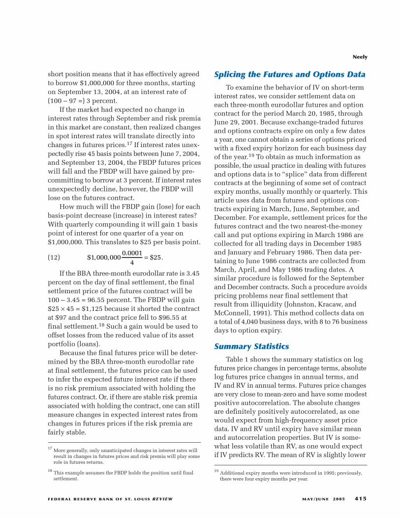
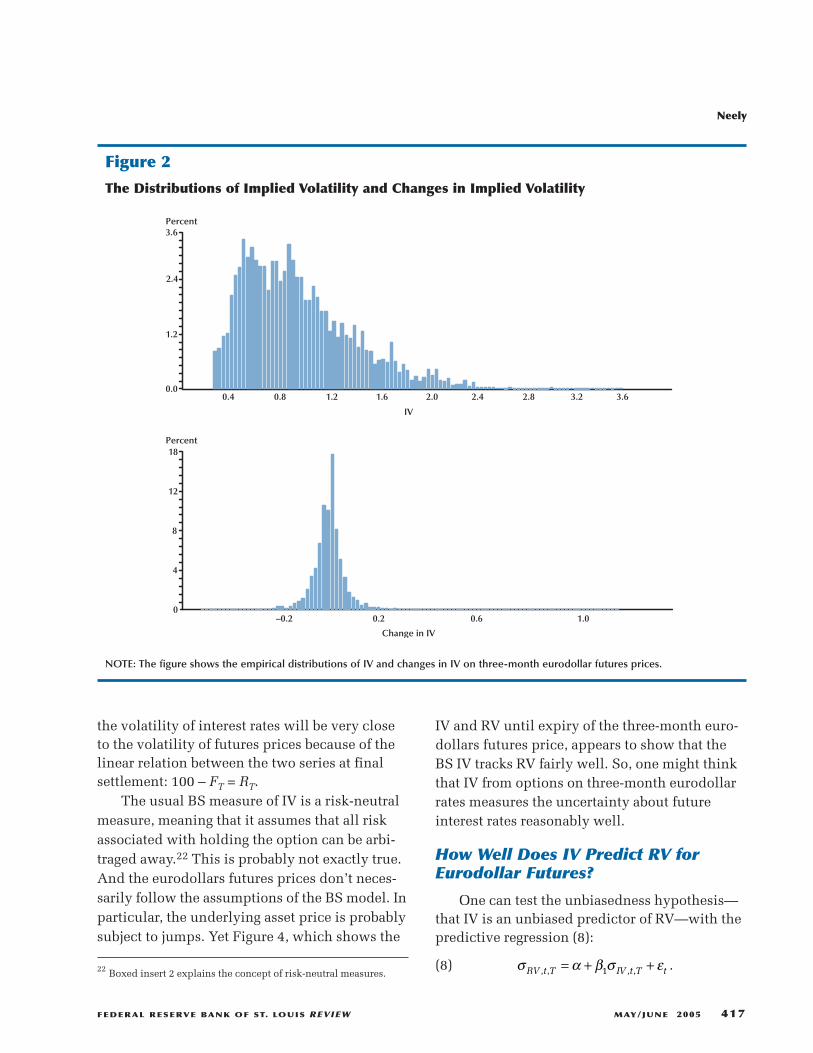
Figure 2 clearly illustrates the right skew-ness in the distribution of IV and changes in IV.Although it is difficult to see in the lower panelof Figure 2, very large positive changes in IV aremuch more common than very large negativechanges in IV. The fact that IV must be positiveprobably partly explains the right skewness inthese distributions.

Eurodollar Rates and the Federal FundsTarget Rate

The futures and options data considered herepertain to three-month eurodollar rates. The Fed,however, is more concerned about the federalfunds rate, the overnight interbank interest rateused to implement monetary policy, than aboutother short-term interest rates, such as the euro-dollar rate.20 This is because the federal fundsfutures prices are often interpreted to providemarket expectations of the Fed’s near-term policyactions. Short-term interest rates are closely tied

together, however, so there might be informationabout the federal funds rate in three-month euro-dollar futures.

Figure 3 shows that, although the three-montheurodollar is much more variable than the federalfunds target over a period of a few days, the twoseries closely tracked each other over periodslonger than a few days from March 1985 throughJune 2001. One can assume that the expected pathof the funds rate is closely related to the expectedpath of the three-month eurodollar rate.21 Andtherefore the IV on three-month eurodollars prob-ably tracks the uncertainty about the federal fundstarget over horizons greater than a few days.

Options on Eurodollar Rates

Because option prices depend on the volatil-ity of the underlying asset (among other factors),one can measure the uncertainty associated withexpectations of future interest rates from IV fromoption prices on eurodollar futures contracts. And

Neely


Table 1Summary Statistics

100 · ln(F(t) /F(t–1)) 249 · 100 · |ln(F(t) /F(t–1))| σIV,t,T σRV,t,T

Total observations 4,040 4,040 4,040 4,040

Nobs 3,975 3,975 3,953 4,039

µ 0.003 10.088 0.953 0.769

σ 0.070 14.141 0.458 0.494

Max 1.272 316.645 3.601 3.861

Min –0.449 0.000 0.251 0.076

ρ1 0.070 0.213 0.986 0.989

ρ2 0.023 0.241 0.973 0.977

ρ3 –0.014 0.226 0.960 0.965

ρ4 –0.025 0.246 0.948 0.954

ρ5 –0.007 0.247 0.936 0.942

NOTE: The table contains summary statistics on log futures price changes (percent), annualized absolute log futures price changes, andannualized IV and RV until expiry. The rows show the total number of observations in the sample, the non-missing observations, the mean,the standard deviation, the maximum, the minimum, and the first five autocorrelations. The standard error of the autocorrelations isabout 1/√T ≈ 0.016.

21 The payoff to the federal funds futures contract depends on theaverage federal funds rate over the course of a month, whereasthe three-month eurodollar futures contract payoff depends on theBBA quote for the three-month eurodollar rate at one point in time,the expiry of the contract.

20 Carlson, Melick, and Sahinoz (2003) describe the recently devel-oped options market on federal funds futures contracts.

the volatility of interest rates will be very closeto the volatility of futures prices because of thelinear relation between the two series at finalsettlement: 100 – FT = RT.

The usual BS measure of IV is a risk-neutralmeasure, meaning that it assumes that all riskassociated with holding the option can be arbi-traged away.22 This is probably not exactly true.And the eurodollars futures prices don’t neces-sarily follow the assumptions of the BS model. Inparticular, the underlying asset price is probablysubject to jumps. Yet Figure 4, which shows the

IV and RV until expiry of the three-month euro-dollars futures price, appears to show that theBS IV tracks RV fairly well. So, one might thinkthat IV from options on three-month eurodollarrates measures the uncertainty about futureinterest rates reasonably well.

How Well Does IV Predict RV forEurodollar Futures?

One can test the unbiasedness hypothesis—that IV is an unbiased predictor of RV—with thepredictive regression (8):

(8) .σ α β σ εRV t T IV t T t, , , ,= + +1

Neely


Percent

Percent

IV

Change in IV

3.6

2.4

1.2

0.0

18

12

8

4

0

0.4 0.8 1.2 1.6 2.0 2.4 2.8 3.2 3.6

–0.2 0.2 0.6 1.0

Figure 2

The Distributions of Implied Volatility and Changes in Implied Volatility

NOTE: The figure shows the empirical distributions of IV and changes in IV on three-month eurodollar futures prices.

22 Boxed insert 2 explains the concept of risk-neutral measures.

Neely


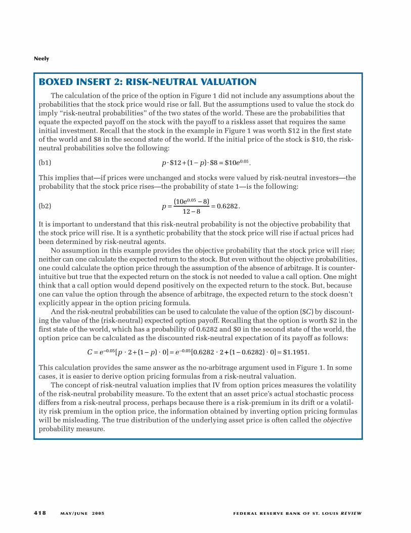
BOXED INSERT 2: RISK-NEUTRAL VALUATIONThe calculation of the price of the option in Figure 1 did not include any assumptions about the

probabilities that the stock price would rise or fall. But the assumptions used to value the stock doimply “risk-neutral probabilities” of the two states of the world. These are the probabilities thatequate the expected payoff on the stock with the payoff to a riskless asset that requires the sameinitial investment. Recall that the stock in the example in Figure 1 was worth $12 in the first stateof the world and $8 in the second state of the world. If the initial price of the stock is $10, the risk-neutral probabilities solve the following:

(b1) .

This implies that—if prices were unchanged and stocks were valued by risk-neutral investors—theprobability that the stock price rises—the probability of state 1—is the following:

(b2) .

It is important to understand that this risk-neutral probability is not the objective probability thatthe stock price will rise. It is a synthetic probability that the stock price will rise if actual prices hadbeen determined by risk-neutral agents.

No assumption in this example provides the objective probability that the stock price will rise;neither can one calculate the expected return to the stock. But even without the objective probabilities,one could calculate the option price through the assumption of the absence of arbitrage. It is counter-intuitive but true that the expected return on the stock is not needed to value a call option. One mightthink that a call option would depend positively on the expected return to the stock. But, becauseone can value the option through the absence of arbitrage, the expected return to the stock doesn’texplicitly appear in the option pricing formula.

And the risk-neutral probabilities can be used to calculate the value of the option ($C) by discount-ing the value of the (risk-neutral) expected option payoff. Recalling that the option is worth $2 in thefirst state of the world, which has a probability of 0.6282 and $0 in the second state of the world, theoption price can be calculated as the discounted risk-neutral expectation of its payoff as follows:

.

This calculation provides the same answer as the no-arbitrage argument used in Figure 1. In somecases, it is easier to derive option pricing formulas from a risk-neutral valuation.

The concept of risk-neutral valuation implies that IV from option prices measures the volatilityof the risk-neutral probability measure. To the extent that an asset price’s actual stochastic processdiffers from a risk-neutral process, perhaps because there is a risk-premium in its drift or a volatil-ity risk premium in the option price, the information obtained by inverting option pricing formulaswill be misleading. The true distribution of the underlying asset price is often called the objectiveprobability measure.

C e p p e= + − = −– . .[ � ( )� ] [ . �0 05 0 052 1 0 0 6282 2?Ê ?Ê ?Ê ++ − =( . )� ] $ .1 0 6282 0 1 1951?Ê

pe= −

−=( )

..10 8

12 80 6282

0 05

p p e?Ê ?Ê$ ( ) $ $ .12 1 8 10 0 05+ − =

For overlapping horizons, the residuals in (8)will be autocorrelated and, while ordinary leastsquares (OLS) estimates are still consistent, theautocorrelation must be dealt with in construct-ing standard errors (Jorion, 1995). Such data setsare described as “telescoping” because correlationbetween adjacent errors declines linearly and thenjumps up at the point at which contracts arespliced.

Table 2 shows the results of estimating (8)with σIV,t,T and σRV,t,T on three-month eurodollarfutures. β̂1 is statistically significantly less than1—0.83—indicating that IV is an overly volatilepredictor of subsequent RV. This is the usualfinding from such regressions: See Canina andFiglewski (1993), Lamoureux and Lastrapes(1993), Jorion (1995), Fleming (1998), Christensenand Prabhala (1998), and Szakmary et al. (2003),for example. As discussed previously, there aremany potential explanations for this conditionalbias—sample selection, overlapping data, errorsin IV—but the most popular story is that stochas-tic volatility introduces risk to delta hedging,making writing options risky.

Figure 5 shows a scatterplot of {IV, RV} pairsalong with the OLS fitted values from Table 2, a45-degree line and the mean of IV and RV. If IVwere an unbiased predictor of RV, the 45-degreeline would be the true relation between them.The fact that the OLS line is flatter than the 45-degree line illustrates that IV is an overly volatilepredictor of RV. The cross in Figure 5—which iscentered on {mean IV, mean RV}—lies beneaththe 45-degree line, illustrating that the mean IVis higher than mean RV.

What Does IV Illustrate AboutUncertainty About Future Interest Rates?

Comparing Figure 3 with Figure 4 shows thatIV has been declining with the overall level ofshort-term interest rates, which have been fallingwith inflation since the early 1980s. One interpre-tation of the data is that the sharp rise in inflationin the 1970s and the subsequent disinflation ofthe 1980s created much uncertainty about thelevel of future interest rates, which has graduallyfallen over the past 20 years. The reduction inuncertainty with respect to interest rates probably

Neely


Eurodollar

Federal Funds

14

12

10

8

6

4

2

0

Percent

1984 1989 1994 1999 2004

Figure 3

Federal Funds Targets and Three-MonthEurodollar Rates

NOTE: The figure displays federal funds targets and the three-month eurodollar rate from January 1, 1984, to July 25, 2003.

IV

RV

4.0

3.2

2.4

1.6

0.8

0.0

Percent

1984 1988 1996 2000 20041992

Figure 4

Realized and Implied Volatility on Three-Month Eurodollar Rates

NOTE: The figure displays three-month eurodollar IV and RVfrom March 20, 1985, through June 29, 2001.

stems from both a reduction in the level of interestrates and greater certainty about both monetarypolicy and the level of real economic activity.

A close look at Figure 4 also hints that theremight be some seasonal pattern in IV, associatedwith the expiry of contracts. Indeed, long-horizonIVs tend to be larger than short-horizon IVs (which,for brevity, are not shown). As IV is scaled to beinterpretable as an annual measure, comparableat any horizon, this is a bit of a mystery. It mightsimply be an artifact of the simplifying assump-tions of the BS model.

What Sort of News Is Coincident withChanges in IV?

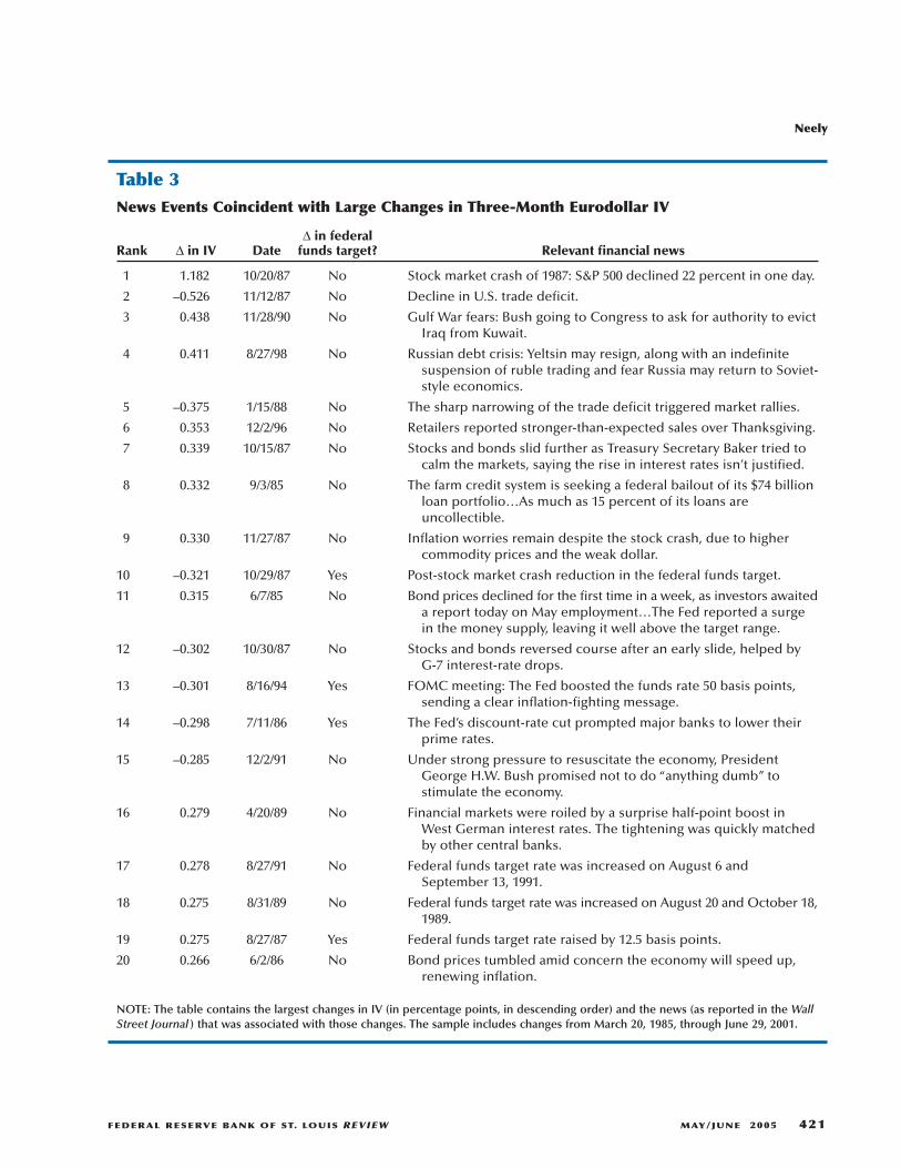
Events of obvious economic importance andlarge changes in the futures price, itself, oftenaccompany the largest changes in IV. To examinenews events around large changes, the Wall StreetJournal business section was searched for newson the dates of large changes and on the daysimmediately following those changes—from

March 20, 1985, through June 29, 2001. Table 3shows some of the largest changes in IV duringthe sample and the event that might have precip-itated it.

The largest change in IV, by far, is a rise of1.2 percentage points on October 20, 1987, coin-ciding with the stock market crash of 1987, whenthe S&P 500 lost 22 percent of its value in oneday. Four more of the top 20 changes (includingthe second largest) happened in the six weeksfollowing the crash and one happened eight weeksbefore the crash, on August 27, 1987. The largechanges in the IV of three-month eurodollar inter-est rates reflected uncertainty about future interestrates prior to the crash. A change in FederalReserve Chairmen might have fueled the apparentuncertainty about the economy and the stance ofmonetary policy. Alan Greenspan took office asChairman of the Board of Governors of the FederalReserve on August 11, 1987.

The third largest change, a 0.44-percentage-point increase, occurred on November 28, 1990.It coincided with reports that President GeorgeH.W. Bush would go to Congress to ask for endorse-ment of plans to use military force to evict Iraqiforces from Kuwait. The possibility of war in suchan economically important area of the worldclearly spooked financial markets.

Neely


Table 2Predicting Realized Volatility with ImpliedVolatility

α̂ –0.017

(s.e.) 0.052

β̂1 0.834

(s.e.) 0.064

Wald 40.814

Wald PV 0.000

Observations 3,952

R2 0.599

NOTE: The table shows the results of predicting three-montheurodollar RV with IV, as in (8). The rows show α̂ , its robuststandard error, β̂1 , its robust standard error, the Wald teststatistic for the null that {α, β } = {0, 1}, the Wald test p-value,the number of observations, and the R2 of the regression.

RV until Expiry

IV

4.0

3.2

2.4

1.6

0.8

0.00.4 0.8 1.6 2.0 2.41.2 2.8 3.2 3.6 4.0

Figure 5

Implied Volatility as a Predictor of RealizedVolatility

NOTE: The figure shows a scatterplot of {IV, RV} pairs alongwith the ordinary least-squares fitted values from Table 2 (solidblack line), a 45-degree line (short dashes) and the IV and RV(cross). The data are in percentage terms.

Neely


Table 3News Events Coincident with Large Changes in Three-Month Eurodollar IV

∆ in federal Rank ∆ in IV Date funds target? Relevant financial news

1 1.182 10/20/87 No Stock market crash of 1987: S&P 500 declined 22 percent in one day.

2 –0.526 11/12/87 No Decline in U.S. trade deficit.

3 0.438 11/28/90 No Gulf War fears: Bush going to Congress to ask for authority to evictIraq from Kuwait.

4 0.411 8/27/98 No Russian debt crisis: Yeltsin may resign, along with an indefinite suspension of ruble trading and fear Russia may return to Soviet-style economics.

5 –0.375 1/15/88 No The sharp narrowing of the trade deficit triggered market rallies.

6 0.353 12/2/96 No Retailers reported stronger-than-expected sales over Thanksgiving.

7 0.339 10/15/87 No Stocks and bonds slid further as Treasury Secretary Baker tried to calm the markets, saying the rise in interest rates isn’t justified.

8 0.332 9/3/85 No The farm credit system is seeking a federal bailout of its $74 billion loan portfolio…As much as 15 percent of its loans are uncollectible.

9 0.330 11/27/87 No Inflation worries remain despite the stock crash, due to higher commodity prices and the weak dollar.

10 –0.321 10/29/87 Yes Post-stock market crash reduction in the federal funds target.

11 0.315 6/7/85 No Bond prices declined for the first time in a week, as investors awaiteda report today on May employment…The Fed reported a surge in the money supply, leaving it well above the target range.

12 –0.302 10/30/87 No Stocks and bonds reversed course after an early slide, helped by G-7 interest-rate drops.

13 –0.301 8/16/94 Yes FOMC meeting: The Fed boosted the funds rate 50 basis points, sending a clear inflation-fighting message.

14 –0.298 7/11/86 Yes The Fed’s discount-rate cut prompted major banks to lower their prime rates.

15 –0.285 12/2/91 No Under strong pressure to resuscitate the economy, President George H.W. Bush promised not to do “anything dumb” to stimulate the economy.

16 0.279 4/20/89 No Financial markets were roiled by a surprise half-point boost in West German interest rates. The tightening was quickly matched by other central banks.

17 0.278 8/27/91 No Federal funds target rate was increased on August 6 and September 13, 1991.

18 0.275 8/31/89 No Federal funds target rate was increased on August 20 and October 18,1989.

19 0.275 8/27/87 Yes Federal funds target rate raised by 12.5 basis points.

20 0.266 6/2/86 No Bond prices tumbled amid concern the economy will speed up, renewing inflation.

NOTE: The table contains the largest changes in IV (in percentage points, in descending order) and the news (as reported in the WallStreet Journal ) that was associated with those changes. The sample includes changes from March 20, 1985, through June 29, 2001.

Another large increase, of 0.41 percentagepoints, occurred on August 28, 1998. This rise wascoincident with the Russian debt crisis, rumorsthat President Yeltsin had resigned, and the pos-sibility of a reversal of Russian political andeconomic reforms. The Russian debt crisis hadpotentially serious implications for internationalinvestors. Neely (2004c) discusses the episodeand its potential effect on U.S. financial markets.

Several of the 20 largest changes in three-month eurodollar IV were also associated withlarge changes in the futures price. It is likely thatthese changes in the futures price were unantici-pated because large, anticipated changes in futuresprices provide profit-making opportunities.Additionally, anticipated changes are unlikely tocause a substantial revision to IV. Four of the 20largest changes in IV were also associated withpresumably unanticipated changes in the federalfunds target rate. It seems that unanticipatedmonetary policy can be an important determinantof uncertainty about future interest rates.

Finally, one might note that the large IVchanges shown in Table 3 refute the BS assump-tions of a constant or even continuous volatilityprocess. As such, they might be partly responsiblefor delta hedging errors, which require a riskpremium that causes IV to be a conditionallybiased estimate of RV.

CONCLUSIONThis article has explained the concept of IV

and applied it to measure uncertainty aboutthree-month eurodollar rates. The IVs associatedwith three-month eurodollars can be interpretedto reflect uncertainty about the Federal Reserve’sprimary monetary policy instrument, the federalfunds target rate.

As with IV in most financial markets, the IVof the three-month eurodollar rate has been anoverly volatile predictor of RV. IV on the three-month eurodollar rates has been declining since1985, as inflation and interest rates have fallenand the Fed has gained credibility with financialmarkets. The largest changes in IV were coincidentwith important economic events such as the stock-market crash of 1987, fears of war in the Persian

Gulf, and the Russian debt crisis. Most of the restof the largest changes in IV have similarly beenassociated with important news about the realeconomy or the stock market or revisions toexpected monetary policy.

REFERENCESAng, Andrew; Hodrick, Robert J.; Xing, Yuhang and

Zhang, Xiaoyan. “The Cross-Section of Volatilityand Expected Returns.” Unpublished manuscript,Columbia University, 2003.

Barone-Adesi, Giovanni and Whaley, Robert E.“Efficient Analytic Approximation of AmericanOption Values.” Journal of Finance, 1987, 42, pp.301-20.

Bates, David S. “Testing Option Pricing Models,” inG.S. Maddala and C.R. Rao, eds., Statistical Methodsin Finance/Handbook of Statistics. Volume 14.Amsterdam: Elsevier Publishing, 1996.

Bates, David S. “Post-’87 Crash Fears in the S&P 500Futures Option Market.” Journal of Econometrics,2000, 94, pp. 181-238.

Bates, David S. “Empirical Option Pricing: ARetrospection.” Journal of Econometrics, 2003,116, pp. 387-404.

Beckers, Stan. “Standard Deviations Implied inOptions Prices as Predictors of Futures Stock PriceVariability.” Journal of Banking and Finance, 1981,5, pp. 363-81.

Benzoni, Luca. “Pricing Options Under StochasticVolatility: An Empirical Investigation.” Unpublishedmanuscript, Carlson School of Management, 2002.

Black, Fischer. “The Pricing of Commodity Contracts.”Journal of Financial Economics, 1976, 3, pp. 167-79.

Black, Fischer and Scholes, Myron. “The Valuationof Option Contracts and a Test of Market Efficiency.”Journal of Finance, 1972, 27, pp. 399-417.

Blair, Bevan J.; Poon, Ser-Huang and Taylor, StephenJ. “Forecasting S&P 100 Volatility: The IncrementalInformation Content of Implied Volatilities and

Neely


High-Frequency Index Returns.” Journal ofEconometrics, 2001, 105, pp. 5-26.

Bollerslev, Tim and Zhou, Hao. “Volatility Puzzles: AUnified Framework for Gauging Return-VolatilityRegressions.” Finance and Economics DiscussionSeries 2003-40, Board of Governors of the FederalReserve System, 2003.

Boyle, Phelim and Boyle, Feidhlim. Derivatives: TheTools that Changed Finance. London: Risk Books,2001.

Campbell, John Y. “Intertemporal Asset Pricing with-out Consumption Data.” American EconomicReview, 1993, 83, pp. 487-512.

Canina, Linda and Figlewski, Stephen. “TheInformational Content of Implied Volatility.”Review of Financial Studies, 1993, 6, pp. 659-81.

Carlson, John B.; Melick, William R. and SahinozErkin Y. “An Option for Anticipating Fed Action.”Federal Reserve Bank of Cleveland EconomicCommentary, September 1, 2003, pp. 1-4.

Chernov, Mikhail. “On the Role of Volatility RiskPremia in Implied Volatilities Based ForecastingRegressions.” Unpublished manuscript, ColumbiaUniversity, 2002.

Christensen, B.J. and Prabhala, N.R. “The RelationBetween Implied and Realized Volatility.” Journalof Financial Economics, 1998, 50, pp. 125-50.

Dubofsky, David A. and Miller Jr, Thomas M.Derivatives: Valuation and Risk Management.New York: Oxford University Press, 2003.

Fleming, Jeff. “The Quality of Market VolatilityForecasts Implied by S&P 100 Index OptionPrices.” Journal of Empirical Finance, 1998, 5, pp.317-45.

Heston, Steven L. “A Closed-Form Solution forOptions with Stochastic Volatility with Applicationsto Bond and Currency Options.” Review of FinancialStudies, 1993, 6, pp. 327-43.

Hull, John C. Options, Futures, and Other Derivatives.5th edition. Upper Saddle River, NJ: Prentice Hall,2002.

Hull, John C. and White, Alan. “The Pricing ofOptions on Assets with Stochastic Volatilities.”Journal of Finance, 1987, 42, pp. 281-300.

Jarrow, Robert and Turnbull, Stuart. DerivativeSecurities. Cincinnati, OH: South-Western CollegePublishing, 2000.

Johnston, E.; Kracaw, W. and McConnell, J. “Day-of-the-Week Effects in Financial Futures: An Analysisof GNMA, T-Bond, T-Note, and T-Bill Contracts.”Journal of Financial and Quantitative Analysis,1991, 26, pp. 23-44.

Jorion, Philippe. “Predicting Volatility in the ForeignExchange Market.” Journal of Finance, 1995, 50,pp. 507-28.

Kroner, Kenneth F.; Kneafsey, Kevin P. and Claessens,Stijn. “Forecasting Volatility in CommodityMarkets.” Working Paper 93-3, University ofArizona, 1993.

Krueger, Joel T. and Kuttner, Kenneth N. “The FedFunds Futures Rate as a Predictor of Federal ReservePolicy,” Working Paper WP-95-4, Federal ReserveBank of Chicago, March 1995.

Lamoureux, Christopher G. and Lastrapes, WilliamD. “Forecasting Stock-Return Variance: Toward anUnderstanding of Stochastic Implied Volatilities.”Review of Financial Studies, 1993, 6, pp. 293-326.

Latane, Henry A. and Rendleman, Richard J. Jr.“Standard Deviations of Stock Price Ratios Impliedin Option Prices.” Journal of Finance, 1976, 31,pp. 369-81.

Li, Kai. “Long-Memory versus Option-ImpliedVolatility Prediction.” Journal of Derivatives, 2002,9, pp. 9-25.

Martens, Martin and Zein, Jason. “PredictingFinancial Volatility: High-Frequency Time-SeriesForecasts vis-à-vis Implied Volatility.” Journal ofFutures Markets, 2004, 24(11), pp. 1005-28.

Merton, Robert C. “An Intertemporal Capital AssetPricing Model.” Econometrica, 1973a, 41, pp. 867-87.

Neely


Merton, Robert C. “Theory of Rational Option Pricing.”Bell Journal of Economics, 1973b, 4(1), pp. 141-83.

Neely, Christopher J. “Realignments of Target ZoneExchange Rate Systems: What Do We Know?”Federal Reserve Bank of St. Louis Review,September/October 1994, 76(5), pp. 23-34.

Neely, Christopher J. “Forecasting Foreign ExchangeVolatility: Why Is Implied Volatility Biased andInefficient? And Does It Matter?” Working Paper2002-017D, Federal Reserve Bank of St. Louis, 2004a.

Neely, Christopher J. “Implied Volatility from Optionson Gold Futures: Do Econometric Forecasts AddValue or Simply Paint the Lilly?” Working Paper2003-018C, Federal Reserve Bank of St. Louis, 2004b.

Neely, Christopher J. “The Federal Reserve Respondsto Crises: September 11th Was Not the First.”Federal Reserve Bank of St. Louis Review, March/April 2004c, 86(2), pp. 27-42.

Pakko, Michael R. and Wheelock, David. “MonetaryPolicy and Financial Market Expectations: WhatDid They Know and When Did They Know It?”Federal Reserve Bank of St. Louis Review, July/August 1996, 78(4), pp. 19-32.

Pan, Jun. “The Jump-Risk Premia Implicit in Options:Evidence from an Integrated Time-Series Study.”Journal of Financial Economics, 2002, 63, pp. 3-50.

Poteshman, Allen M. “Forecasting Future Volatilityfrom Option Prices.” Unpublished manuscript,Department of Finance, University of Illinois atUrbana-Champaign, 2000.

Romano, Marc and Touzi, Nizar. “Contingent Claimsand Market Completeness in a Stochastic VolatilityModel.” Mathematical Finance, 1997, 7, pp. 399-410.

Rose, Andrew K. and Svensson, Lars E.O. “Expectedand Predicted Realignments: The FF/DM ExchangeRate During the EMS.” International FinanceDiscussion Paper Number 395, Board of Governorsof the Federal Reserve System, April 1991.

Rose, Andrew K. and Svensson, Lars E.O. “EuropeanExchange Rate Credibility Before the Fall.” NBERWorking Paper No. 4495, National Bureau ofEconomic Research, October 1993.

Shleifer, Andrei, and Vishny, Robert W. “The Limits ofArbitrage.” Journal of Finance, 1997, 54, pp. 35-55.

Svensson, Lars E.O. “The Simplest Test of TargetZone Credibility.” IMF Staff Papers, September1991, pp. 655-65.

Szakmary, Andrew; Ors, Evren; Kim, Jin Kyoung andDavidson, Wallace N. III. “The Predictive Power ofImplied Volatility: Evidence from 35 FuturesMarkets.” Journal of Banking and Finance, 2003,27, pp. 2151-75.

Wilmott, Paul; Howison, Sam and Dewynne, Jeff.The Mathematics of Financial Derivatives: AStudent Introduction. Cambridge: CambridgeUniversity Press, 1995.

Wilmott, Paul. Paul Wilmott on QuantitativeFinance. Chichester, UK: John Wiley & Sons, 2000.

Neely


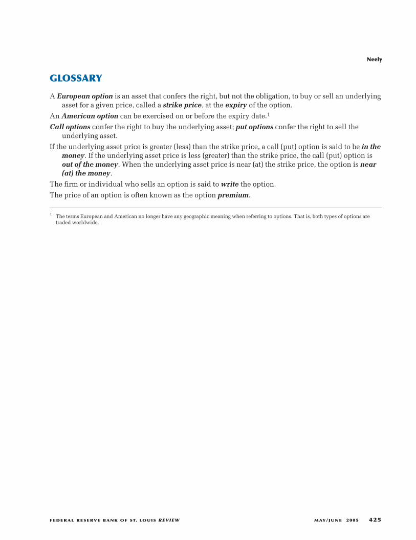
GLOSSARY

A European option is an asset that confers the right, but not the obligation, to buy or sell an underlyingasset for a given price, called a strike price, at the expiry of the option.

An American option can be exercised on or before the expiry date.1

Call options confer the right to buy the underlying asset; put options confer the right to sell theunderlying asset.

If the underlying asset price is greater (less) than the strike price, a call (put) option is said to be in themoney. If the underlying asset price is less (greater) than the strike price, the call (put) option isout of the money. When the underlying asset price is near (at) the strike price, the option is near(at) the money.

The firm or individual who sells an option is said to write the option.

The price of an option is often known as the option premium.

1 The terms European and American no longer have any geographic meaning when referring to options. That is, both types of options aretraded worldwide.

Neely


Using Implied Volatility to Measure Uncertainty About ... · PDF fileFEDERAL RESERVE BANK OF...

Documents

Transcript of Using Implied Volatility to Measure Uncertainty About ... · PDF fileFEDERAL RESERVE BANK OF...