White Paper

WEBSITE: www.jdsu.com/test

Introduction

Traditionally, optical power meters (OPMs) have been used for measuring absolute power, relative to popular standards, such as National Institute of Standards (NIST) or for relative measurements, such as insertion loss or return loss.

Measuring more complex characteristics, such as switch settling time, cross talk, amplifier response, and device rise or fall times require signal conversion from the optical domain to electrical domain using optical-to-electrical (O-E) converters and high-speed oscilloscopes. Advances in OPM technology have rendered such O-E conversions unnecessary, as now transient measurements can be performed purely in the optical domain.

Applications and Standards

A variety of applications can benefit from measuring transient optical signals in the optical domain. Figure 1 shows a high-resolution settling time measurement of an optical signal in the optical domain with repeatable, high fidelity results. Some of the applicable International Electrotechnical Commission (IEC) standards include 61300-3-21, which refers to timing aspects and IEC 61300-3-28, which refers to transient loss. The applications are numerous, and device capability determines the novel and unique measurement implementations, including the following:

• deviceundertest(DUT)settlingtime

• DUTcrosstalk

• DUTrisetime

• DUTfalltime

• synchronization

• stability

• linkrecoverytime

• performancecomparison(forexample,comparingsequentialswitchingtorandomswitching)

Using High-Speed Optical Power Meters for Effective Optical Domain Transient Signal Measurements

Figure 1: Measuring settling time in the optical domain

White Paper: Using High-Speed Optical Power Meters 2

Making Optical Transient Measurements Possible

A few features of an optical power meter make optical transient signal measurement possible. Each feature and its advantages are described below.

Storage Memory/Buffer

Supporting OPMs have a built-in buffer to store data points internally. The amount of storage directly impacts both the measurement resolution as well as the amount of time for which data can be collected.

Averaging Time

Minimum sampling time and averaging time are not always the same. The MOPM-B1 series OPMs can perform a power sample every 4 µs, whereas the minimum averaging time is 20 µs. Choosing a specific averaging time will dictate the number of samples averaged to produce one value. For instance, an averaging time of 20 µs results in a single measurement that is the average of 20/4 = 5 sample points. Typically higher averaging times are chosen to reduce noise in measurements.

For perspective, consider the following scenario:

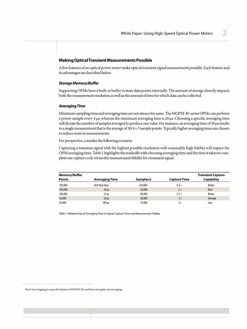
Capturing a transient signal with the highest possible resolution with reasonably high fidelity will impact the OPM averaging time. Table 1 highlights the tradeoffs with choosing averaging time and the time it takes to com-plete one capture cycle versus the measurement fidelity for a transient signal.

Memory/Buffer Transient Capture Points Averaging Time Samples/s Capture Time Capability

100,000 N/A Real time1 250,000 0.4 s Better100,000 20 µs 50,000 2 s Best100,000 25 µs 40,000 2.5 s Better50,000 20 µs 50,000 1 s Average50,000 100 µs 10,000 5 s Low

Table 1: Relationship of Averaging Time to Signal Capture Time and Measurement Fidelity

1Real-time logging is a specific feature of MOPM-B1 and does not apply any averaging.

White Paper: Using High-Speed Optical Power Meters 3

Figure 2a: Optical signal sampled at 4 µs

Figure 2b: Optical signal sampled at 1 ms

The above characteristics determine the amount of data captured and the resolution with which it can be captured.However,thisisonlypartofthepuzzle.OPMsusuallyhavevariousgainstagestocaptureopticalsignals at different strengths. Each of these stages behaves differently and dictates the small signal capture capability, which is a critical factor in determining the capture capability of an OPM.

It is important to have a general idea of the characteristic of the signal being measured. Choosing a higher averaging time can result in averaging values that may not capture the true characteristics of the signal. Figures 2a and 2b best depict the impact of averaging time on capturing true signal characteristics. Figure 2a shows the measurementofasignalmodulatedat100kHzwith50-percentdutycycleanddepth,usingthelowestpossiblesamplingtimeof4µswithnoaveraging(onlyavailableinReal-TimeDataLoggingmodeinMOPM-B1). Figure 2b shows the measurement of the same signal with 1 ms averaging time, showing less information about the source signal.

White Paper: Using High-Speed Optical Power Meters 4

Gain Stages and Analog Bandwidth

OPMs with high-speed logging capability usually have internal analog-to-digital converters for capturing the analog optical signal and storing it as a digital value in memory, along with related signal conditioning circuitry. The measurement capability is limited by the applicable gain stage (dictated by signal strength) and associated circuitry,suchasfilters.Usually,gainstagetransitionscausetheOPMstodiscardsamplesforacertainlengthoftime, allowing for continuity in the acquired data, referred to as blanking time.

Table 2 shows the analog bandwidth of each gain stage capability with MOPM-B1 General Purpose and Premium Performance variants, along with the blanking time per stage.

Analog bandwidth is an especially important consideration when conducting measurements that are essentially step functions. The higher the analog bandwidth at a given gain stage, the better approximated the sharp signal transitions will be in the final measurement.

Gain Stage Power Min (dBm) Power Max (dBm) Blanking Time Between Analog Bandwidth Gain Stages (ms)

1 (min gain) −8 11 1.24 284 kHz2 −26 −6 1.24 21.2 kHz3 −42 −24 1.24 2840 Hz4 −59 −40 20.8 159 Hz5 (max gain) −80 −57 138 24 Hz

Table 2: Example of gain stages, associated power bands, blanking time, and analog bandwidth

Figures 3a and 3b show the measurement of a signal that closely resembles a step function. This measurement wasmadeusingMOPM-B1setinGainStage1(GS1)withanapplicableanalogbandwidthof284kHz,rangingin power from −8 to 11 dBm, with an expected signal power of −2.5 dBm. The measurement was set up to trigger on the rising edge when the input signal strength exceeded the lower bounds of GS 1 or −8 dBm. The pretrigger points enable the capture of data points before the trigger event, as Figure 3a clearly shows. Figure 3b shows the close up signal between −8 and −2.5 dBm.

Figure 3a: Optical Step Function measurement in MOPM-B1 Gain Stage 1

White Paper: Using High-Speed Optical Power Meters 5

Figure 3a: Optical Step Function measurement in MOPM-B1 Gain Stage 1

Figure 3b: Close-up view of Optical Step Function measurement in MOPM-B1 Gain Stage 1

To highlight the impact of analog bandwidth on such step function type measurements refer to Figures 4a and 4b below. The same instrument was set up to operate in Gain Stage 2 (GS 2), −6 to −26 dBm, with an applicable analogbandwidthof21.2kHz,significantlylessthaninGS1at284kHz.Theexpectedsignalpowerinthiscaseis−12 dBm.

The difference in characteristics described in Figures 3 and 4 indicate the importance of setting up step function measurementsaccordingtotheinputsignaltoensurethatresultsrepresentthetruebehavioroftheDUT.

Figure 4a: Optical Step Function measurement in MOPM-B1 Gain Stage 2 Figure 4b: Close-up view of Optical Step Function measurement in MOPM-B1 Gain Stage 2

White Paper: Using High-Speed Optical Power Meters 6

High accuracy logging measurements should typically not be made in Automatic Gain Setting mode. Instead, ensure that the setup falls into the bounds of the applicable gain stage, even if this requires tweaking the measure-ment setup. If, however, a higher dynamic range is required, note that the blanking time applies between gain stage transitions, having a minor impact on the results. A long-term stability measurement with a high averaging time would not be subjected to the above limitations, as the blanking times would be negligible in comparison.

Forperspective,considerthefollowingscenariousingMOPM-B1.Tomeasureatleast10kHzwiththesignalstrength ranging between −3 and −13 dBm requires taking such a measurement at its highest, where the signal is measured in GS 1, and at its lowest, where it is measured in GS 2. This technique will not yield accurate results because of the blanking time restraint between gain stages.

The suggested method requires using an attenuator to bring the range into GS 2 and attenuate it by 6 dB to ensure a signal in the range of −9 and −19 dBm, capable of detection within one gain stage.

Measuring a sinusoidal signal, or a signal with some frequency characteristic similar to mechanical vibrations of an optical switch as it comes into rest position, requires ensuring that the sampling is at least twice as fast as the signal to avoid aliasing. Figure 2a shows a modulated signal measured appropriately, whereas Figure 2b illus-trates the affects of aliasing by choosing an unsuitable averaging and sampling time.

Forinstance,measuringasignalwithcharacteristicsat100kHzobviouslyrequiresoperatingatGS1withtheanalogbandwidthof284kHz.Asignallevelwellbelow−8dBmwouldmakeoperatinginthatrangedifficult.Insuch cases, the signal level could be tweaked by amplifying the signal, to ensure it fits in GS 1.

Another important consideration is the difference between lowest possible averaging time and lowest possible sampling time. For instance, the highest measurement speed available in MOPM-B1 is in Real-Time mode, which exports the sample at every 4 µs, whereas the minimum averaging time is 20 µs. This mode allows for the highest sampling speed, but gain stage limitations and blanking time constraints still apply.

Triggering

Triggering capability is perhaps one of the most important features of transient captures as it is not always pos-sible to know exactly when an event will occur in time to set logging to capture the effects. Therefore, using a triggering mechanism is ideal for starting such a measurement.

Achangecan trigger logging.Historically, analog transistor-to-transistor logic (TTL) triggershavebeensupported to start OPM measurements. This method typically still poses the limitations of O-E and E-O conver-sions. Some OPMs can trigger based on a set time delay from a logging start event.

Triggering on the rising or falling edge, with configurable power threshold levels, can be a very useful method for capturing measurements, much like on digital sampling oscilloscopes.

One very important feature of a scope is its ability to view data in negative time, relative to a triggered event cap-ture, referred to as a pretrigger. While triggering enables the capture of data from the start of a specific event, it does not show the history of the signal, which is particularly useful when assessing settling times.

White Paper: Using High-Speed Optical Power Meters 7

Additional Considerations

Data Transfer Speed and Capacity

Intoday’slocalareanetwork(LAN)extensioninterfaceforinstrumentation(LXI)-basedworld,instrumentscommunicate over TCI/IP, requiring their own IP addresses. While Transmission Control Protocol/Internet Protocol (TCP/IP)-based communication can be much faster than traditional General Purpose Interface Bus (GPIB), the problem is IP addresses are becoming harder to acquire in most lab and manufacturing environ-ments and often require several cycles of request and approval with a respective IT division. Therefore, device densityhelpsreducethenumberofinstrumentIPaddressesrequired.Useofmultithreadedtestapplicationscancleverly manage the data transfer speed.

Remote Control Capability

Theabilitytoremotelyviewinstrumentsinremotelocationsprovidesaveryusefulfeature.LXI-compliantOPMsprovidethisabilityaboveandbeyondTCP/IPsupportinginstruments.LXIcompliancerequirestheabil-ity to view and control instruments remotely, while some vendors even provide rich graphical user interfaces (GUIs)thatofferremoteaccess.Thisfeaturecanbeveryconvenientandespeciallyusefulindistributeddevelop-ment environments.

Application Examples

The next few examples show common transient measurements of interest to designers. The measurement set-tings are provided as a guideline to indicate appropriate setup for each transient type. These examples have been generatedusingMOPM-B1andtheJDSUOPMscope™application.

Real-Time Data Logging

This example is based on a sinusoidal wave source connected directly with MOPM-B1 (device 4) that is set for data logging in Real-Time mode. Table 3 describes the applicable measurement parameters.

Parameter Applicable Setting

Acquisition Acquisition = Logging Data points = 100,000 (Max) Averaging time = Real-Time (4 µs) Note: Acquisition tab displays the total time the measurement will takeTrigger Enabled = False Device = NA Pretrigger = NA Edge = NA Level = NADevice Atime = 20 µs (This is the value displayed, although samples are taken at 4 µs) GS (gain stage) = 1Control Tab Run = Selected (causes button state change to STOP)

Table 3: Real-Time Logging Parameter settings

White Paper: Using High-Speed Optical Power Meters 8

Figure5showstheresultscapturedusingReal-timeDataLoggingcapabilitywith100,000datapointscollectedfor each channel at 4 µs/sample, resulting in a total capture time of 0.4 s. It shows the close-up view of the real-time measurement of the optical sinusoidal signal. The markers can be used to indicate signal characteristics, such as period.

Figure 5: Real-Time Sinusoidal Signal measurement

Trigger on Rising Edge

This example is based on a continuous wave source connected directly with MOPM-B1 (device 4) that is pow-ered On from the Off state with logging enabled when the power level rises above −8 dBm. This threshold was set to ensure measurements confined to GS 1. Table 4 describes the applicable measurement parameters.

Parameter Applicable Setting

Acquisition Acquisition = Logging Data points = 100,000 (Max) Averaging time = 20 µs (Minimum possible)Trigger Enabled = True Device 4 = True, all others = False Pretrigger = 0 (points to capture before trigger event) Edge = Rising Level = −8 dBm (threshold to trigger when signal rises above this value)Device Atime = 20 µs (automatically set when selecting averaging time from Acquisition tab) GS (gain stage) = 1Control Tab Run = Selected (causes button state change to STOP)

Table 4: Parameter settings for logging on rising edge trigger

White Paper: Using High-Speed Optical Power Meters 9

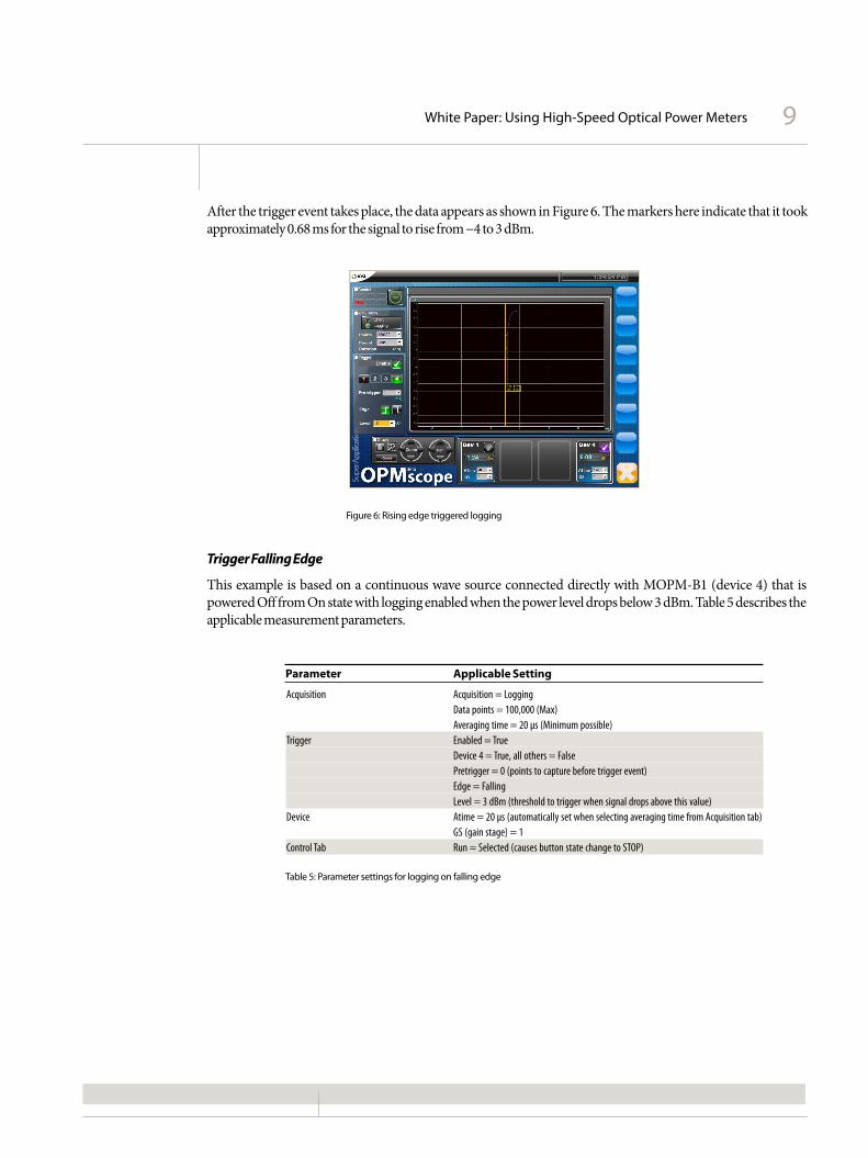
After the trigger event takes place, the data appears as shown in Figure 6. The markers here indicate that it took approximately 0.68 ms for the signal to rise from −4 to 3 dBm.

Figure 6: Rising edge triggered logging

Trigger Falling Edge

This example is based on a continuous wave source connected directly with MOPM-B1 (device 4) that is powered Off from On state with logging enabled when the power level drops below 3 dBm. Table 5 describes the applicable measurement parameters.

Parameter Applicable Setting

Acquisition Acquisition = Logging Data points = 100,000 (Max) Averaging time = 20 µs (Minimum possible)Trigger Enabled = True Device 4 = True, all others = False Pretrigger = 0 (points to capture before trigger event) Edge = Falling Level = 3 dBm (threshold to trigger when signal drops above this value)Device Atime = 20 µs (automatically set when selecting averaging time from Acquisition tab) GS (gain stage) = 1Control Tab Run = Selected (causes button state change to STOP)

Table 5: Parameter settings for logging on falling edge

White Paper: Using High-Speed Optical Power Meters 10

Post processing steps make it possible to see in Figure 7 that the signal dropped below 3 dBm to a value of less than −45 dBm in less than approximately 1 ms. However, a better way to capture such data in these instances uses pretriggers to show a history of the event before the trigger point, as described in the following example.

Parameter Applicable Setting

Acquisition Acquisition = Logging Data points = 100,000 (Max, although the device adjusts for the number of pretrigger points) Averaging time = 20 µs (Minimum possible)Trigger Enabled = True Device 4 = True, all others = False Pretrigger = 10,000 (points to capture before trigger event) Edge = Falling Level = 3 dBm (threshold to trigger when signal drops above this value)Device Atime = 20 µs (automatically set when selecting averaging time from Acquisition tab) GS (gain stage) = 1Control Tab Run = Selected (causes button state change to STOP)

Table 6: Parameter settings for falling edge logging with pretrigger points

Figure 7: Falling edge triggered logging

Triggering on Falling Edge with Pretrigger Data Points

This example is based on a continuous wave source connected directly with MOPM-B1 (device 4) that is powered Off from On state with logging enabled when the power level drops below 3 dBm. Pretrigger points are selected to view the history before the trigger event. Table 6 describes the applicable measurement parameters.

White Paper: Using High-Speed Optical Power Meters 11

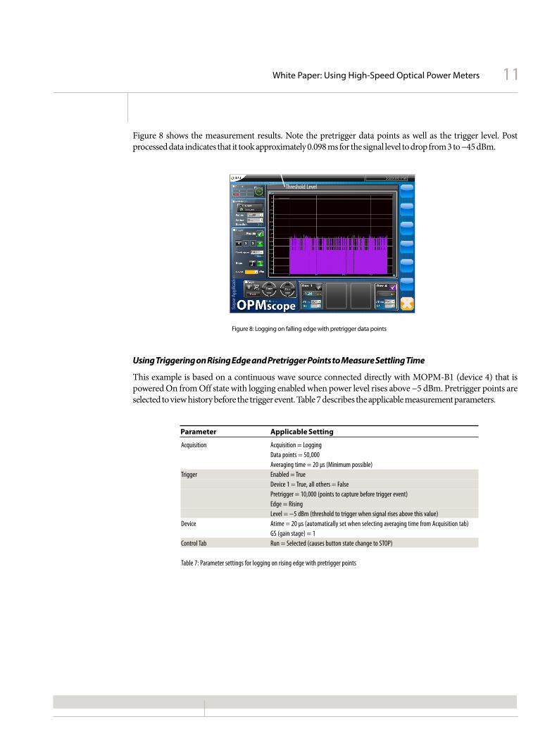
Figure 8: Logging on falling edge with pretrigger data points

Figure 8 shows the measurement results. Note the pretrigger data points as well as the trigger level. Post processed data indicates that it took approximately 0.098 ms for the signal level to drop from 3 to −45 dBm.

Using Triggering on Rising Edge and Pretrigger Points to Measure Settling Time

This example is based on a continuous wave source connected directly with MOPM-B1 (device 4) that is powered On from Off state with logging enabled when power level rises above −5 dBm. Pretrigger points are selected to view history before the trigger event. Table 7 describes the applicable measurement parameters.

Parameter Applicable Setting

Acquisition Acquisition = Logging Data points = 50,000 Averaging time = 20 µs (Minimum possible)Trigger Enabled = True Device 1 = True, all others = False Pretrigger = 10,000 (points to capture before trigger event) Edge = Rising Level = −5 dBm (threshold to trigger when signal rises above this value)Device Atime = 20 µs (automatically set when selecting averaging time from Acquisition tab) GS (gain stage) = 1Control Tab Run = Selected (causes button state change to STOP)

Table 7: Parameter settings for logging on rising edge with pretrigger points

Pretrigger Points

Threshold Level

Test & Measurement Regional Sales

NORTH AMERICATEL: 1 866 228 3762FAX: +1 301 353 9216

LATIN AMERICATEL: +1 954 688 5660FAX: +1 954 345 4668

ASIA PACIFICTEL:+852 2892 0990FAX:+852 2892 0770

EMEATEL:+49 7121 86 2222FAX:+49 7121 86 1222

WEBSITE: www.jdsu.com/test

White Paper: Using High-Speed Optical Power Meters 12

Productspecificationsanddescriptionsinthisdocumentsubjecttochangewithoutnotice.©2010JDSUniphaseCorporation301682130000810MOPM.WP.LAB.TM.AE August2010

Figure 9 shows the result of the measurement. Post process data reveals that from the trigger event, it took 4.48msforthesignaltostabilizeat−1.25dBm.

Figure10showsthemeasurementresultsforamotorizedmechanicalopticalswitcharmwiththesamemeasurement settings and shows how long it took for the switch to settle.

Figure 9: Logging on rising edge trigger with pretrigger data points Figure 10: Logging on rising edge trigger with pretrigger data points showing switch settling