63

Using GeoGebra as an Expressive Modeling Tool: Discovering the

Anatomy of the Cycloid’s Parametric Equation

Tolga KABACA1, Muharrem AKTUMEN2

1PhD. Pamukkale University, Faculty of Education, Denizli, TURKEY

2PhD. Ahi Evran University, Faculty of Education, Kirsehir, TURKEY

tkabaca@pau.edu.tr aktumen@gmail.com

ABSTRACT. In Greek geometry, curves were defined as objects, which are geometric and static. For example, a parabola is defined as the intersection of a cone and plane like other conics, which are first introduced by Apollonius of Perga (262 BC – 190 BC). Alternatively, 17th century European mathematicians have preferred to define the curves as the trajectory of a moving point. In his Dialogue Concerning Two New Science of 1638, Galileo found the trajectory of a canon ball. Assuming a vacuum, the trajectory is a parabola (Barbin, 1996). We can understand that some of the scientists, who studied on curves, actually were interested in the problems of applied science, like Galileo as an astronomer and a physician, Nicholas of Cusa as an astronomer etc. Some of the scientist, who lived approximately in the same century, took further the research on the curves as a mathematician (e.g. Roberval, Mersenne, Descartes and Wren).

1. Introduction

In our time, dynamically capable software GeoGebra provides us an innovative opportunity to investigate and understand the curves described as dynamically. GeoGebra can be thought as an innovative mathematical modeling tool. After a comprehensive literature synthesis about modeling by using technology, Doer and Pratt propose two kinds of modeling according to the learners’ activity; “exploratory modeling” and “expressive modeling” (Doer and Pratt, 2008).

64

A learner uses a ready model, which is constructed by an expert, in exploratory modeling, while he or she shows their own performance to construct the model in expressive modeling. During the process of constructing the model, learner can find the opportunity to reveal the way of understanding the relationship between the real world and the model world (Doer and Pratt, 2008). We can also derive from this view that the expressive modeling also has the potential of assessing some unexpected teaching and learning opportunities. By the view of expressive modeling approach, giving the task of “construct the cycloid curve without using its formal equation” to our students will be more useful than presenting a ready cycloid graph, even if it is also dynamic. Students will encounter some problem, which most of them are mathematical, and in the process of solving these they will have several learning opportunities for some special cases, sometimes unexpected. In this paper, a process of constructing a sequence of dynamic GeoGebra applets is described. In the First part, entitled “Producing the Cycloid with GeoGebra”, describes how we can demonstrate the animation of cycloid by using only a circle with any radius and a point, rotating around this circle. The second part is devoted to understand the formal equation of cycloid by the help of dynamic visual opportunities, provided by GeoGebra. In the third part, it will be revealed that how we can obtain new kind of cycloids with same rolling circle but with different movements and what the relationship between movement and equation is. Last, we will have an answer to the question “Why do we need to parametric functions, while we know a lot about Cartesian functions?” which is meaningful for a novice calculus student.

2. Producing the Cycloid with GeoGebra:

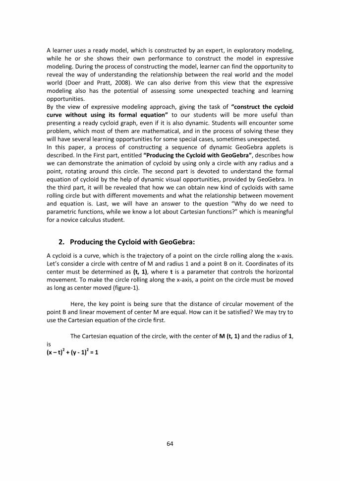
A cycloid is a curve, which is the trajectory of a point on the circle rolling along the x-axis. Let’s consider a circle with centre of M and radius 1 and a point B on it. Coordinates of its center must be determined as (t, 1), where t is a parameter that controls the horizontal movement. To make the circle rolling along the x-axis, a point on the circle must be moved as long as center moved (figure-1).

Here, the key point is being sure that the distance of circular movement of the point B and linear movement of center M are equal. How can it be satisfied? We may try to use the Cartesian equation of the circle first.

The Cartesian equation of the circle, with the center of M (t, 1) and the radius of 1,

is (x – t)

2 + (y - 1)

2 = 1

65

Figure-1: First draft for the construction of cycloid

After representing the point B as (x, y), we need to rearrange the coordinates x and y in terms of the parameter t. Because, the horizontal movement depends on the parameter t and we must make connection between the movement of center and the point B. But, this effort will be invalid to solve the following challenges;

1- Challenge of solving x and y in terms of parameter t directly. 2- Challenge of being sure that the distance of circular movement of the point B and linear movement of center M are equal. It will be better to use an alternative representation of the point B on the circle.

Let’s use a polar representation of point B. Consider a vertical constant line segment MB1 and let the parameter t controls the clockwise angle M (figure-2).

Figure-2: Second draft for the construction of cycloid

Position of the circle and the point B for t=0

Position of the circle and the point B for t=2

Position of the circle and the point B for t=

B

M Direction of movement

Rolling direction of the point B Rolling direction of

the point B

(t, 1)

(t, 1)

(x, y)

(x, y)

66

This approach will overcome the challenge of solving x and y in terms of parameter t. Since both angle M and the point M depends on parameter t, we can control both the point B and the circle by manipulating the parameter t. This approach has also the potential of making students aware of the importance of polar representation.

The second challenge still remains. How can we be sure that the distance of circular movement of the point B and linear movement of center M are equal? The answer of this question also hosts an opportunity of making students aware of the difference between the degree and the radian, which are alternative angle units.

The default angle unit of GeoGebra is degree. This causes a problem of controlling two variables, which one is an angle and the other one is a distance, with the same parameter t. Please make your students to remember the meaning of radian is “Radian is the measure of an angle M, which is corresponding to the length of circular arc of a unit circle, whose center is M.”

So, by changing the default angle unit as radian in GeoGebra and defining the

interval of slider, which controls the value of parameter t, as from 0 to 2, you can obtain a proper cycloid curve. You can see the curve by making the point B trace on and animating the slider (Figure-3).

Figure-3: Cycloid curve by obtaining the trace of the point B, which is on the unit circle rolling over the

x-axis1

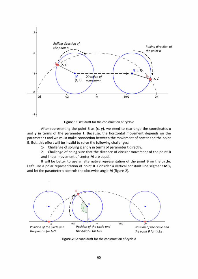
We can enrich the understanding the relation between the radian as an angle measure and as a circular arc length by changing the radius, while keeping the rotation measure as the parameter t (Figure-4)2.

After creating a slider r controlling the radius of the rolling circle, we can observe that while the radius increases the trace of the point B does not look like a cycloid, at least a part of it (figure-4). What is the reason?

1 You can reach the ggb applet from http://tolgakabaca.pau.edu.tr/cycloid/cycloid1.html and the construction

protocol in the appendix 2 When you add a slider r controlling the radius of the circle, you need to redefine the circle as Circle[M, r] by using

the object properties dialog box. By this way, you will make the circle still rolling over the x-axis, with radius r.

67

Figure-4: Cycloid-similar curves by obtaining the trace of the point B, which is on the circle with

radius-r3

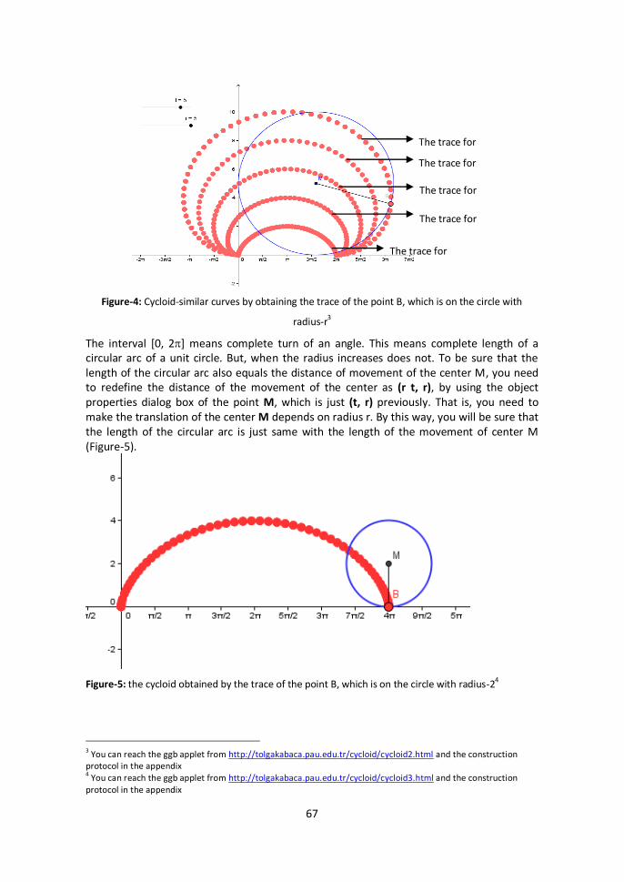
The interval [0, 2] means complete turn of an angle. This means complete length of a circular arc of a unit circle. But, when the radius increases does not. To be sure that the length of the circular arc also equals the distance of movement of the center M, you need to redefine the distance of the movement of the center as (r t, r), by using the object properties dialog box of the point M, which is just (t, r) previously. That is, you need to make the translation of the center M depends on radius r. By this way, you will be sure that the length of the circular arc is just same with the length of the movement of center M (Figure-5).

Figure-5: the cycloid obtained by the trace of the point B, which is on the circle with radius-24

3 You can reach the ggb applet from http://tolgakabaca.pau.edu.tr/cycloid/cycloid2.html and the construction

protocol in the appendix 4 You can reach the ggb applet from http://tolgakabaca.pau.edu.tr/cycloid/cycloid3.html and the construction

protocol in the appendix

The trace for r=1

The trace for r=2

The trace for r=3

The trace for r=4

The trace for r=5

68

3. Discovering the equation of the cycloid:

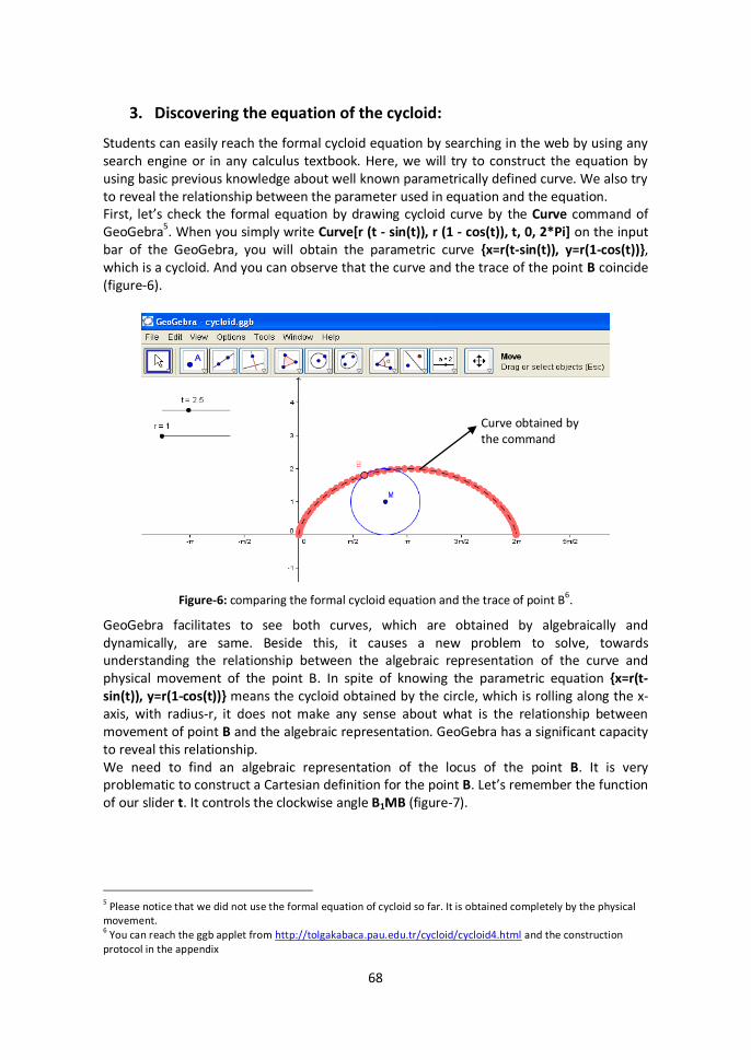
Students can easily reach the formal cycloid equation by searching in the web by using any search engine or in any calculus textbook. Here, we will try to construct the equation by using basic previous knowledge about well known parametrically defined curve. We also try to reveal the relationship between the parameter used in equation and the equation. First, let’s check the formal equation by drawing cycloid curve by the Curve command of GeoGebra5. When you simply write Curve[r (t - sin(t)), r (1 - cos(t)), t, 0, 2*Pi] on the input bar of the GeoGebra, you will obtain the parametric curve {x=r(t-sin(t)), y=r(1-cos(t))}, which is a cycloid. And you can observe that the curve and the trace of the point B coincide (figure-6).

Figure-6: comparing the formal cycloid equation and the trace of point B6.

GeoGebra facilitates to see both curves, which are obtained by algebraically and dynamically, are same. Beside this, it causes a new problem to solve, towards understanding the relationship between the algebraic representation of the curve and physical movement of the point B. In spite of knowing the parametric equation {x=r(t-sin(t)), y=r(1-cos(t))} means the cycloid obtained by the circle, which is rolling along the x-axis, with radius-r, it does not make any sense about what is the relationship between movement of point B and the algebraic representation. GeoGebra has a significant capacity to reveal this relationship. We need to find an algebraic representation of the locus of the point B. It is very problematic to construct a Cartesian definition for the point B. Let’s remember the function of our slider t. It controls the clockwise angle B1MB (figure-7).

5 Please notice that we did not use the formal equation of cycloid so far. It is obtained completely by the physical

movement. 6 You can reach the ggb applet from http://tolgakabaca.pau.edu.tr/cycloid/cycloid4.html and the construction

protocol in the appendix

Curve obtained by the command

69

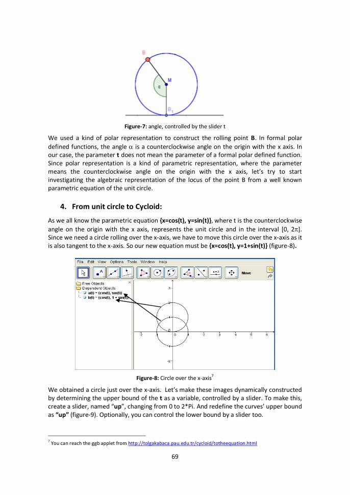
Figure-7: angle, controlled by the slider t

We used a kind of polar representation to construct the rolling point B. In formal polar

defined functions, the angle is a counterclockwise angle on the origin with the x axis. In our case, the parameter t does not mean the parameter of a formal polar defined function. Since polar representation is a kind of parametric representation, where the parameter means the counterclockwise angle on the origin with the x axis, let’s try to start investigating the algebraic representation of the locus of the point B from a well known parametric equation of the unit circle.

4. From unit circle to Cycloid:

As we all know the parametric equation {x=cos(t), y=sin(t)}, where t is the counterclockwise

angle on the origin with the x axis, represents the unit circle and in the interval [0, 2]. Since we need a circle rolling over the x-axis, we have to move this circle over the x-axis as it is also tangent to the x-axis. So our new equation must be {x=cos(t), y=1+sin(t)} (figure-8).

Figure-8: Circle over the x-axis7

We obtained a circle just over the x-axis. Let’s make these images dynamically constructed by determining the upper bound of the t as a variable, controlled by a slider. To make this, create a slider, named “up”, changing from 0 to 2*Pi. And redefine the curves’ upper bound as “up” (figure-9). Optionally, you can control the lower bound by a slider too.

7 You can reach the ggb applet from http://tolgakabaca.pau.edu.tr/cycloid/totheequation.html

70

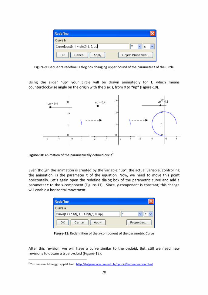
Figure-9: GeoGebra redefine Dialog box changing upper bound of the parameter t of the Circle

Using the slider “up” your circle will be drawn animatedly for t, which means counterclockwise angle on the origin with the x axis, from 0 to “up” (Figure-10).

Figure-10: Animation of the parametrically defined circle8

Even though the animation is created by the variable “up”, the actual variable, controlling the animation, is the parameter t of the equation. Now, we need to move this point horizontally. Let’s again open the redefine dialog box of the parametric curve and add a parameter t to the x-component (Figure-11). Since, y-component is constant; this change will enable a horizontal movement.

Figure-11: Redefinition of the x-component of the parametric Curve

After this revision, we will have a curve similar to the cycloid. But, still we need new revisions to obtain a true cycloid (Figure-12).

8 You can reach the ggb applet from http://tolgakabaca.pau.edu.tr/cycloid/totheequation.html

71

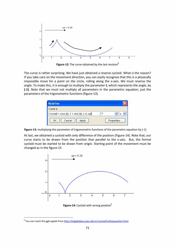
Figure-12: The curve obtained by the last revision8

The curve is rather surprising. We have just obtained a reverse cycloid. What is the reason? If you take care on the movement direction, you can easily recognize that this is a physically impossible move for a point on the circle, rolling along the x-axis. We must reverse the angle. To make this, it is enough to multiply the parameter t, which represents the angle, by (-1). Note that we must not multiply all parameters in the parametric equation, just the parameters of the trigonometric functions (figure-13).

Figure-13: multiplying the parameter of trigonometric functions of the parametric equation by (-1)

At last, we obtained a cycloid with only difference of the position (Figure-14). Note that, our curve starts to be drawn from the position that parallel to the x-axis. But, the formal cycloid must be started to be drawn from origin. Starting point of the movement must be changed as in the figure-15

Figure-14: Cycloid with wrong position9

9 You can reach the ggb applet from http://tolgakabaca.pau.edu.tr/cycloid/totheequation.html

72

To make the movement starting from the origin it is enough to ad /2 to the parameter, which controls the angle. After this last change we will have the parametric

equation {x=t+cos(-(t+/2)), y=1+sin(-(t+/2))} and we will have a complete formal cycloid (Figure-16).

Figure-15: Starting point of the angle must be revised as in the right

After this revision you will have the figure-16 by animating the slider “up”.

Figure-16: Complete cycloid which have the parametric equation {x=t+cos(-(t+/2)), y=1+sin(-

(t+/2))}10

From now on, we have to make an algebraically revision to reach the formal form of the obtained equation. Let’s write the parametric equation more explicitly as below;

cos(-( / 2))

1 sin(-( / 2))

x t t

y t

……………………………………………….[1]

10

You can reach the ggb applet from http://tolgakabaca.pau.edu.tr/cycloid/totheequation.html

73

Since cosine and sine functions are even and odd functions respectively, the equation [1] can be revised as below;

cos( / 2)

1 - sin( / 2)

x t t

y t

……………………………………………….[2]

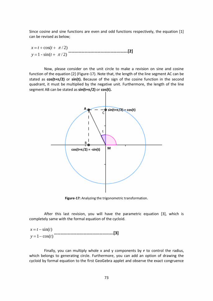
Now, please consider on the unit circle to make a revision on sine and cosine

function of the equation [2] (Figure-17). Note that, the length of the line segment AC can be

stated as cos(t+/2) or sin(t). Because of the sign of the cosine function in the second quadrant, it must be multiplied by the negative unit. Furthermore, the length of the line

segment AB can be stated as sin(t+/2) or cos(t).

Figure-17: Analyzing the trigonometric transformation.

After this last revision, you will have the parametric equation [3], which is completely same with the formal equation of the cycloid.

sin( )

1 cos( )

x t t

y t

……………………………………………….[3]

Finally, you can multiply whole x and y components by r to control the radius,

which belongs to generating circle. Furthermore, you can add an option of drawing the cycloid by formal equation to the first GeoGebra applet and observe the exact congruence

t

sin(t+/2) = cos(t)

cos(t+/2) = -sin(t) M

A

B

C

74

of both drawing, with rolling circle and formal equation (it was obtained in the figure-6, before understanding the relationship).

5. Survey to the new Curves:

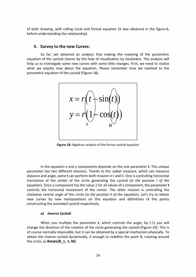
So far, we obtained an analysis that making the meaning of the parametric equation of the cycloid clearer by the help of visualization by GeoGebra. This analysis will help us to investigate some new curves with some little changes. First, we need to realize what we exactly now about the equation. Please remember how we reached to the parametric equation of the cycloid (Figure-18).

Figure-18: Algebraic analysis of the formal cycloid equation

In the equation x and y components depends on the one parameter t. This unique parameter has two different missions. Thanks to the radian measure, which can measure distance and angle, same t can perform both mission in I and II. One is controlling horizontal translation of the center of the circle generating the cycloid (in the position I of the equation). Since y component has the value 1 for all values of x component, the parameter t controls the horizontal movement of the center. The other mission is controlling the clockwise central angle of this circle (in the position II of the equation). Let’s try to obtain new curves by new manipulations on this equation and definitions of the points constructing the animated cycloid respectively.

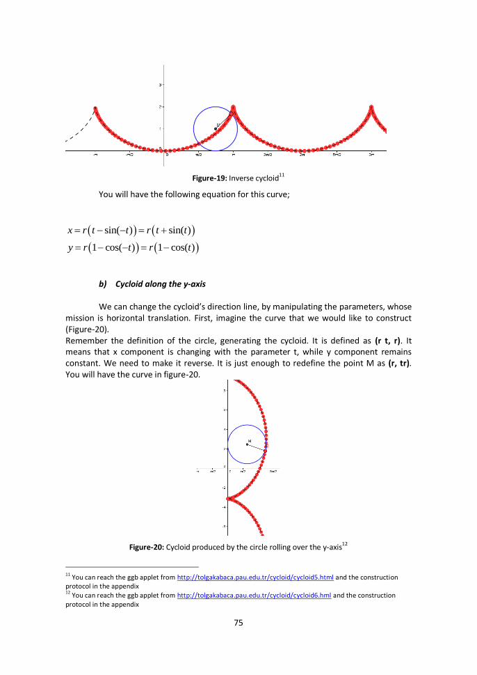
a) Inverse Cycloid

When you multiply the parameter t, which controls the angle, by (-1) you will

change the direction of the rotation of the circle generating the cycloid (Figure-19). This is of course normally impossible, but it can be obtained by a special mechanism physically. To obtain the inverse cycloid dynamically, it enough to redefine the point B, rotating around the circle, as Rotate[B_1, -t, M]

sin( )

1 cos( )

x r t t

y r t

I II

75

Figure-19: Inverse cycloid11

You will have the following equation for this curve;

sin( ) sin( )

1 cos( ) 1 cos( )

x r t t r t t

y r t r t

b) Cycloid along the y-axis

We can change the cycloid’s direction line, by manipulating the parameters, whose mission is horizontal translation. First, imagine the curve that we would like to construct (Figure-20). Remember the definition of the circle, generating the cycloid. It is defined as (r t, r). It means that x component is changing with the parameter t, while y component remains constant. We need to make it reverse. It is just enough to redefine the point M as (r, tr). You will have the curve in figure-20.

Figure-20: Cycloid produced by the circle rolling over the y-axis12

11

You can reach the ggb applet from http://tolgakabaca.pau.edu.tr/cycloid/cycloid5.html and the construction protocol in the appendix 12

You can reach the ggb applet from http://tolgakabaca.pau.edu.tr/cycloid/cycloid6.hml and the construction protocol in the appendix

76

The equation of this curve can be constructed by same revision on translation of

the center;

1 sin( )

cos( )

x r t

y r t t

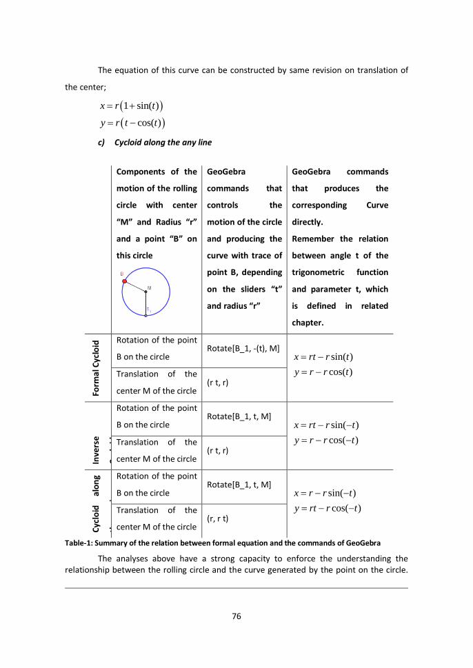
c) Cycloid along the any line

Components of the

motion of the rolling

circle with center

“M” and Radius “r”

and a point “B” on

this circle

GeoGebra

commands that

controls the

motion of the circle

and producing the

curve with trace of

point B, depending

on the sliders “t”

and radius “r”

GeoGebra commands

that produces the

corresponding Curve

directly.

Remember the relation

between angle t of the

trigonometric function

and parameter t, which

is defined in related

chapter.

Form

al C

yclo

id Rotation of the point

B on the circle Rotate[B_1, -(t), M]

sin( )

cos( )

x rt r t

y r r t

Translation of the

center M of the circle (r t, r)

Inve

rse

Cyc

loid

Rotation of the point

B on the circle Rotate[B_1, t, M]

sin( )

cos( )

x rt r t

y r r t

Translation of the

center M of the circle (r t, r)

Cyc

loid

al

on

g

the

y-ax

is

Rotation of the point

B on the circle Rotate[B_1, t, M]

sin( )

cos( )

x r r t

y rt r t

Translation of the

center M of the circle (r, r t)

Table-1: Summary of the relation between formal equation and the commands of GeoGebra

The analyses above have a strong capacity to enforce the understanding the relationship between the rolling circle and the curve generated by the point on the circle.

77

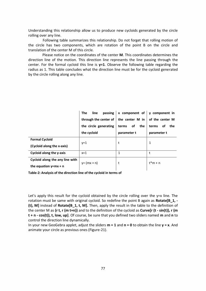
Understanding this relationship allow us to produce new cycloids generated by the circle rolling over any line.

Following table summarizes this relationship. Do not forget that rolling motion of the circle has two components, which are rotation of the point B on the circle and translation of the center M of this circle.

Please notice on the coordinates of the center M. This coordinates determines the direction line of the motion. This direction line represents the line passing through the center. For the formal cycloid this line is y=1. Observe the following table regarding the radius as 1. This table concludes what the direction line must be for the cycloid generated by the circle rolling along any line.

The line passing

through the center of

the circle generating

the cycloid

x component of

the center M in

terms of the

parameter t

y component in

of the center M

terms of the

parameter t

Formal Cycloid

(Cycloid along the x-axis) y=1 t 1

Cycloid along the y-axis x=1 1 t

Cycloid along the any line with

the equation y=mx + n y= (mx + n) t t*m + n

Table-2: Analysis of the direction line of the cycloid in terms of

Let’s apply this result for the cycloid obtained by the circle rolling over the y=x line. The rotation must be same with original cycloid. So redefine the point B again as Rotate[B_1, -(t), M] instead of Rotate[B_1, t, M]. Then, apply the result in the table to the definition of the center M as (r t, r (m t+n)) and to the definition of the cycloid as Curve[r (t - sin(t)), r (m t + n - cos(t)), t, low, up]. Of course, be sure that you defined two sliders named m and n to control the direction line dynamically. In your new GeoGebra applet, adjust the sliders m = 1 and n = 0 to obtain the line y = x. And animate your circle as previous ones (Figure-21).

78

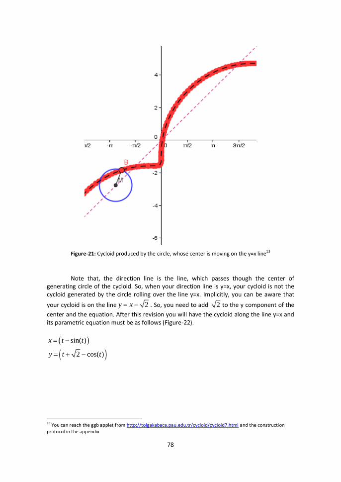
Figure-21: Cycloid produced by the circle, whose center is moving on the y=x line13

Note that, the direction line is the line, which passes though the center of generating circle of the cycloid. So, when your direction line is y=x, your cycloid is not the cycloid generated by the circle rolling over the line y=x. Implicitly, you can be aware that

your cycloid is on the line 2y x . So, you need to add 2 to the y component of the

center and the equation. After this revision you will have the cycloid along the line y=x and its parametric equation must be as follows (Figure-22).

sin( )

2 cos( )

x t t

y t t

13

You can reach the ggb applet from http://tolgakabaca.pau.edu.tr/cycloid/cycloid7.html and the construction protocol in the appendix

79

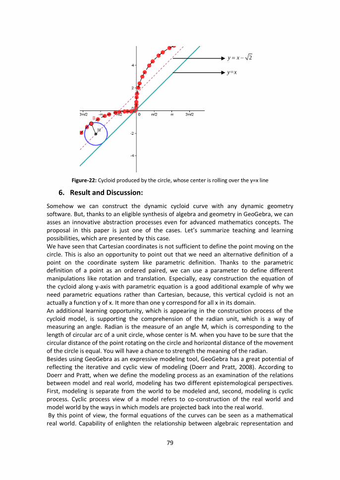
Figure-22: Cycloid produced by the circle, whose center is rolling over the y=x line

6. Result and Discussion:

Somehow we can construct the dynamic cycloid curve with any dynamic geometry software. But, thanks to an eligible synthesis of algebra and geometry in GeoGebra, we can asses an innovative abstraction processes even for advanced mathematics concepts. The proposal in this paper is just one of the cases. Let’s summarize teaching and learning possibilities, which are presented by this case. We have seen that Cartesian coordinates is not sufficient to define the point moving on the circle. This is also an opportunity to point out that we need an alternative definition of a point on the coordinate system like parametric definition. Thanks to the parametric definition of a point as an ordered paired, we can use a parameter to define different manipulations like rotation and translation. Especially, easy construction the equation of the cycloid along y-axis with parametric equation is a good additional example of why we need parametric equations rather than Cartesian, because, this vertical cycloid is not an actually a function y of x. It more than one y correspond for all x in its domain. An additional learning opportunity, which is appearing in the construction process of the cycloid model, is supporting the comprehension of the radian unit, which is a way of measuring an angle. Radian is the measure of an angle M, which is corresponding to the length of circular arc of a unit circle, whose center is M. when you have to be sure that the circular distance of the point rotating on the circle and horizontal distance of the movement of the circle is equal. You will have a chance to strength the meaning of the radian. Besides using GeoGebra as an expressive modeling tool, GeoGebra has a great potential of reflecting the iterative and cyclic view of modeling (Doerr and Pratt, 2008). According to Doerr and Pratt, when we define the modeling process as an examination of the relations between model and real world, modeling has two different epistemological perspectives. First, modeling is separate from the world to be modeled and, second, modeling is cyclic process. Cyclic process view of a model refers to co-construction of the real world and model world by the ways in which models are projected back into the real world. By this point of view, the formal equations of the curves can be seen as a mathematical real world. Capability of enlighten the relationship between algebraic representation and

2y x

y=x

80

geometric representation of GeoGebra allows us to discover the anatomy of the parametric equation of the cycloid. There is only one parameter, named as t, is used to define both x and y components in the cycloid equation. Our struggle of controlling two different movements (rotation of the point on the circle and translation of the point, which represents the center of the circle) by a unique slider in GeoGebra reveals that parameter t has two different meaning. Decoding this meaning of the equation allows us to create new kinds of cycloids. So, the cycloid model, modeled by GeoGebra with its algebraic capabilities, has constructed the cycloids’ equation in mathematical real world. This construction can be advanced to the other dynamic curves like epicycloids, hypocycloid or asteroid by creative manipulations on coordinates of the center of generating circle, and the rotation of the point on this circle.

References:

- Barbin, E., (1996), The Role of Problems in the History and Teaching of Mathematics, in Vita Mathematica: Historical Research and Integration with teaching, Edited by Ronald Calinger, (pp. 17-25), MAA Notes. 40 - Doerr, H.M. and Pratt, D. (2008), The Learning of Mathematics and Mathematical modeling, In Research on Technology in the Teaching and Learning of Mathematics Volume I: Research Syntheses edited by M. K. Heid, G. W. Blume (pp. 259-285) Information Age Publishing.

Appendixes

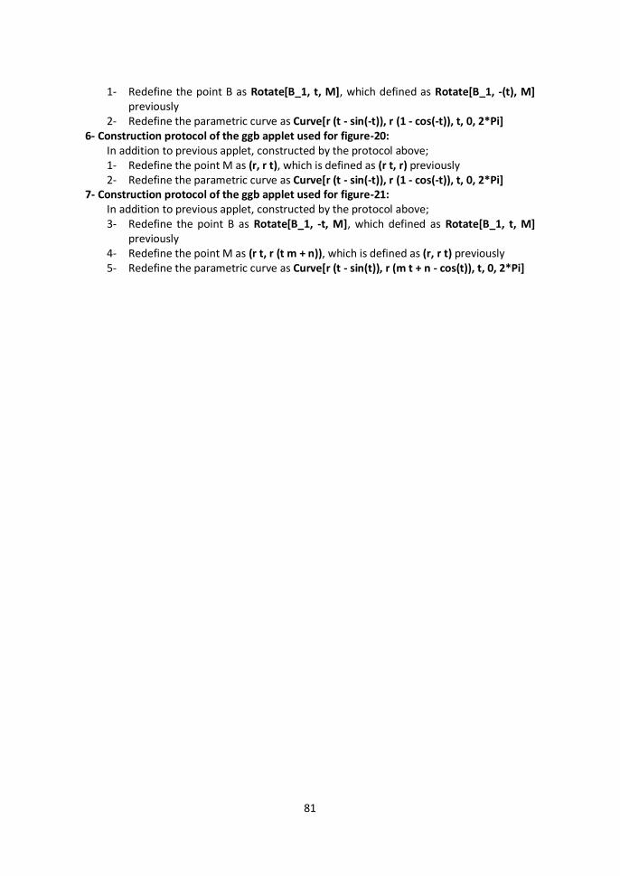
Please note that some details, which makes the applets more stylish (e.g. texts, check boxes, variables controlled by sliders, colors and style of the curves) are omitted in the construction protocols. 1- Construction protocol of the ggb applet generating figure-3:

1- Construct a slider t with the interval [0, 2] (Be sure that it is a number or be sure that default angle measure is set as radian)

2- Define a point M with the coordinate of (t, 1) 3- Define a Circle with the center M and radius 1. 4- Define a point B_1 on the circle with the coordinates of (0, 0) 5- Rotate the point B_1 with the angle t and the center M and rename it as B. 6- Optionally you can construct a line segment from M to B. 7- Hide the point B_1 and make the point B trace on

2- Construction protocol of the ggb applet used for figure-4: In addition to previous applet, constructed by the protocol above; 1- Construct a slider r with the interval [1, 5] 2- Redefine the circle as Circle[M, r], which is defined as Circle[M, 1] previously 3- Redefine the point M as (t, r), which is defined as (t, 1) previously

3- Construction protocol of the ggb applet used for figure-5: In addition to previous applet, constructed by the protocol above; 1- Redefine the point M as (r t, r), which is just defined as (t, r) previously.

4- Construction protocol of the ggb applet used for figure-6: In addition to previous applet, constructed by the protocol above; 1- Construct a parametric curve by using the command Curve[r (t - sin(t)), r (1 -

cos(t)), t, 0, 2*Pi] 5- Construction protocol of the ggb applet used for figure-19:

In addition to previous applet, constructed by the protocol above;

81

1- Redefine the point B as Rotate[B_1, t, M], which defined as Rotate[B_1, -(t), M] previously

2- Redefine the parametric curve as Curve[r (t - sin(-t)), r (1 - cos(-t)), t, 0, 2*Pi] 6- Construction protocol of the ggb applet used for figure-20:

In addition to previous applet, constructed by the protocol above; 1- Redefine the point M as (r, r t), which is defined as (r t, r) previously 2- Redefine the parametric curve as Curve[r (t - sin(-t)), r (1 - cos(-t)), t, 0, 2*Pi]

7- Construction protocol of the ggb applet used for figure-21: In addition to previous applet, constructed by the protocol above; 3- Redefine the point B as Rotate[B_1, -t, M], which defined as Rotate[B_1, t, M]

previously 4- Redefine the point M as (r t, r (t m + n)), which is defined as (r, r t) previously 5- Redefine the parametric curve as Curve[r (t - sin(t)), r (m t + n - cos(t)), t, 0, 2*Pi]

82

Future-Learning2010 3rd International Conference on “Innovations in Learning for the Future 2010: e-Learning” Istanbul University Turkish Informatics Foundation Kültür University Turkish

Informatics Society GeoGebra Institute of Ankara

First Eurasia Meeting of GeoGebra (EMG) May 11-13, 2010

Istanbul-European Capital of Culture 2010, TURKEY http://futurelearning.org.tr

Aim and Scope The use of computers in dynamic and interactive visualizations both in mathematics and mathematics education has been widely accepted. Visualization of the mathematical concepts helps students develop a better understanding of these concepts and provides opportunities to connect with applied sciences. In order to promote conceptual understanding in mathematics, a learning environment is expected to explicit the connections among the concepts and to provide multiple representations in the sense that many scholars described. GeoGebra as a dynamic mathematics software combines numeric, visual, and algebraic representations. It provides multiple representations of mathematical objects and their connections in the graphical, algebraic, and spreadsheet views. Moreover, all these representations are linked dynamically. As the result of research explored the use and benefits of this contemporary environment, a corpus of literature has been accumulated. This Eurasia Meeting of GeoGebra (EMG) will be a right place to share literature and research results as well as to elaborate the ideas emerged in the First International GeoGebra Conference. Furthermore, GeoGebra is free, online, and open source software and is translated into 48 different languages by volunteers. These features of GeoGebra become more valuable if we consider socio-economic structure of the region. Any institute regardless of their economic and geographical circumstances could benefit from GeoGebra and contribute to the pool created by GeoGebra volunteers.