Using Gaussian process regression to denoise images … · 2007-05-08 · remove artefacts from...
74
Using Gaussian process regression to denoise images and remove artefacts from microarray data by Peter Junteng Liu A thesis submitted in conformity with the requirements for the degree of Master of Science Graduate Department of Computer Science University of Toronto Copyright c 2007 by Peter Junteng Liu
Transcript of Using Gaussian process regression to denoise images … · 2007-05-08 · remove artefacts from...
Using Gaussian process regression to denoise images and
remove artefacts from microarray data
by
Peter Junteng Liu
A thesis submitted in conformity with the requirementsfor the degree of Master of Science
Graduate Department of Computer Science
University of Toronto
Copyright c© 2007 by Peter Junteng Liu
Abstract
Using Gaussian process regression to denoise images and remove artefacts from
microarray data
Peter Junteng Liu
Master of Science
Graduate Department of Computer Science
University of Toronto
2007
Natural image denoising is a well-studied problem of computer vision, but still eludes
sufficiently good solutions. Removing spatial artefacts from DNA microarray data is of
significant practical importance to biologists, but overly simple methods are commonly
used. We show that the two seemingly disparate problems of image denoising and spatial
artefact removal from DNA microarrays can be solved using similar algorithms when
the problems are viewed as a decomposition of the data into spatially-independent and
spatially-dependent components. We discuss previously used methods and how Gaussian
processes for regression (GPR) may be used to solve both problems. We present a new
method employing a novel covariance function for use in GPR in the special case of two-
dimensional grid data. Finally, we show that our new method compares well with popular
previous methods in both image denoising and microarray artefact removal applications.
ii

Acknowledgements
I would like to first thank my supervisors, Radford Neal and Brendan Frey, who have
provided excellent mentorship throughout my studies. Your insight is always valuable
and your patience is much appreciated.
This thesis work also benefited significantly from Carl Rasmussen for providing ex-
cellent and free software implementing conjugate-gradients and Gaussian processes; Ofer
Shai for providing microarray data and STR code and explaining it; and Eddie Ng for
presenting NL-Means to me.
Finally, I am indebted to my other colleagues, friends, and family who have provided
support in many forms.
iii

Contents
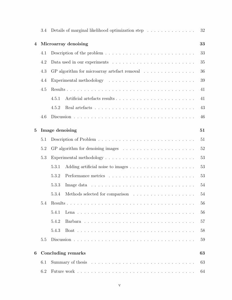
1 Introduction 1
1.1 Noisy grid data . . . . . . . . . . . . . . . . . . . . . . . . . . . . . . . . 1
1.2 Outline of thesis . . . . . . . . . . . . . . . . . . . . . . . . . . . . . . . . 4
2 Related Work 6
2.1 Median filtering . . . . . . . . . . . . . . . . . . . . . . . . . . . . . . . 7
2.2 Mean and Gaussian Filtering . . . . . . . . . . . . . . . . . . . . . . . . 8
2.3 Non-local Means . . . . . . . . . . . . . . . . . . . . . . . . . . . . . . . 9
2.4 Other methods not compared . . . . . . . . . . . . . . . . . . . . . . . . 10
3 Gaussian process method 12
3.1 Using Gaussian processes for noisy 2-dimensional interpolation . . . . . 12
3.1.1 Gaussian process priors . . . . . . . . . . . . . . . . . . . . . . . . 13
3.1.2 Sampling functions from a Gaussian process . . . . . . . . . . . . 15
3.1.3 Gaussian process regression . . . . . . . . . . . . . . . . . . . . . 16
3.1.4 Selecting the covariance function . . . . . . . . . . . . . . . . . . 20
3.1.5 Selecting hyperparameters . . . . . . . . . . . . . . . . . . . . . . 24
3.1.6 Limitations of the 2-d interpolation approach . . . . . . . . . . . 26
3.2 Adding pseudo-inputs to grid data . . . . . . . . . . . . . . . . . . . . . 26
3.2.1 Novel general algorithm for denoising grid data . . . . . . . . . . 29
3.3 Managing the O(N 3) time complexity . . . . . . . . . . . . . . . . . . . 30
iv
3.4 Details of marginal likelihood optimization step . . . . . . . . . . . . . . 32
4 Microarray denoising 33
4.1 Description of the problem . . . . . . . . . . . . . . . . . . . . . . . . . . 33
4.2 Data used in our experiments . . . . . . . . . . . . . . . . . . . . . . . . 35
4.3 GP algorithm for microarray artefact removal . . . . . . . . . . . . . . . 36
4.4 Experimental methodology . . . . . . . . . . . . . . . . . . . . . . . . . 39
4.5 Results . . . . . . . . . . . . . . . . . . . . . . . . . . . . . . . . . . . . . 41
4.5.1 Artificial artefacts results . . . . . . . . . . . . . . . . . . . . . . . 41
4.5.2 Real artefacts . . . . . . . . . . . . . . . . . . . . . . . . . . . . . 43
4.6 Discussion . . . . . . . . . . . . . . . . . . . . . . . . . . . . . . . . . . . 46
5 Image denoising 51
5.1 Description of Problem . . . . . . . . . . . . . . . . . . . . . . . . . . . . 51
5.2 GP algorithm for denoising images . . . . . . . . . . . . . . . . . . . . . 52
5.3 Experimental methodology . . . . . . . . . . . . . . . . . . . . . . . . . . 53
5.3.1 Adding artificial noise to images . . . . . . . . . . . . . . . . . . . 53
5.3.2 Performance metrics . . . . . . . . . . . . . . . . . . . . . . . . . 53
5.3.3 Image data . . . . . . . . . . . . . . . . . . . . . . . . . . . . . . 54
5.3.4 Methods selected for comparison . . . . . . . . . . . . . . . . . . 54
5.4 Results . . . . . . . . . . . . . . . . . . . . . . . . . . . . . . . . . . . . . 56
5.4.1 Lena . . . . . . . . . . . . . . . . . . . . . . . . . . . . . . . . . . 56
5.4.2 Barbara . . . . . . . . . . . . . . . . . . . . . . . . . . . . . . . . 57
5.4.3 Boat . . . . . . . . . . . . . . . . . . . . . . . . . . . . . . . . . . 58
5.5 Discussion . . . . . . . . . . . . . . . . . . . . . . . . . . . . . . . . . . . 59
6 Concluding remarks 63
6.1 Summary of thesis . . . . . . . . . . . . . . . . . . . . . . . . . . . . . . 63
6.2 Future work . . . . . . . . . . . . . . . . . . . . . . . . . . . . . . . . . . 64
v

Bibliography 66
vi
Chapter 1
Introduction
1.1 Noisy grid data
This thesis primarily concerns itself with two-dimensional grid data {(xi, yi)}Ni=1 ⊂ R
2×R,
where xi describes the location of the ith data point on a finite, uniformly-spaced grid,
and yi is its value. We also assume the grid is complete in that every point of the grid has
a data point in our data set. In the spatial statistics literature, this is sometimes called
regular lattice data [4]. A common example of complete grid data is a rectangular image,
where the locations are the pixel row and column indices and the values are the pixel
intensities. Our goal will be to explain each yi as a decomposition into two components,
with one of them, ni, being zero-mean, independent, and identically distributed
yi = si + ni (1.1)
Of course, further assumptions on the behaviour of s and n are necessary to make
the problem meaningful. In our work the s component will have some dependence on
location, whereas the n component will be independent of location. We refrain from the
terms “signal” and “noise” when referring to these components because which component
is actually the noise depends on the context. Instead we think of s and n as short for
spatial (or dependent) and independent, respectively.
1
Chapter 1. Introduction 2
Although there are potentially many applications, we will focus on two:
1. DNA microarray spatial artefact removal: yi is the (log of the) expression level for
probe i on a DNA microarray, si is the contribution from spatial artefacts, and ni
is the true expression level of the probe. xi is the position of probe i on the array.
Here ni is the signal (the independence from location comes from the assumption
that the probes are placed on the array in random order).
2. Natural image denoising: yi is the gray-level of a noisy image at pixel i, si is the
contribution of the true image pixel, and ni is pixel-independent noise. xi is the
position of pixel i in the image. Here si is the signal.
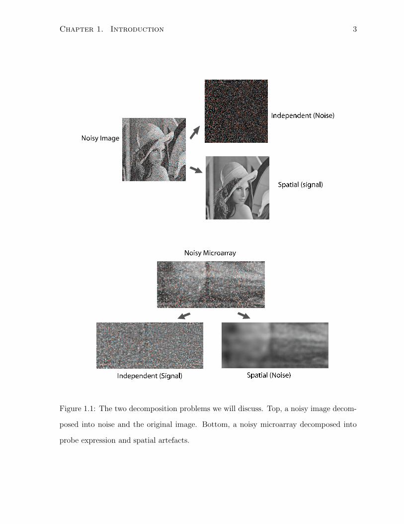
We show schematically an example of each problem in Figure 1.1.
Given the nature of these interpretations of s, informally we expect s to exhibit spatial
regularity or correlations; however, we neither make differentiability nor continuity (as a
function of the spatial variable x) a requirement.
Historically, these two problems have been attacked separately, although the main
difference between them is that in the first case we are interested in the spatially in-
dependent term and in the second in the spatially-dependent term. Because we usually
expect the signal-component to have greater energy than the noise-component, we expect
the independent component to dominate in the case of microarray artefact removal, and
the dependent component to dominate in the case of image denoising.
More importantly, it seems methods designed for either application can be used for
the other with minor modifications. It may be that certain methods really are better for
one application, or that one is best for both. In this thesis we investigate this possibility
by adapting algorithms from both the bioinformatics and image processing communities
to both applications and comparing to our own novel approach using Gaussian process
regression.
Chapter 1. Introduction 3
�����sy Image
����� �� �����t (N
����e)
� ���������l (����������
)
�����sy M
��������������� �
� ���������l (�������� !����� �� ��� �
t (� ���������!
Figure 1.1: The two decomposition problems we will discuss. Top, a noisy image decom-
posed into noise and the original image. Bottom, a noisy microarray decomposed into
probe expression and spatial artefacts.
Chapter 1. Introduction 4
1.2 Outline of thesis
The work described in this thesis began as an application of Gaussian processes to the
problem of denoising microarray image data; however, we realized that the methods
developed for this application could easily be viewed also as natural image denoising
methods. Since there may be interest in our approach from both bioinformatics and
image processing communities, who may have widely differing backgrounds, an attempt
has been made to structure the thesis so that a reader from either community may read
it and learn about our method without learning about the other field. To this end, in
Chapter 2, we present previous methods used to solve either problem. In Chapter 3,
we present a brief introduction to Gaussian processes for regression and a description of
our method. In Chapter 4, we describe the problem of microarray artefact removal and
present some experimental results, using the methods discussed. In Chapter 5, we discuss
the application of these methods to image denoising and present experimental results in
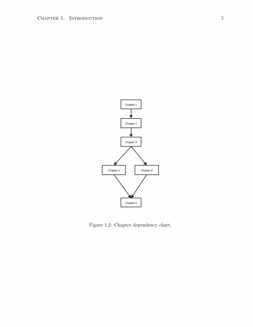
that domain. In Chapter 6, we summarize our contributions and discuss possible future
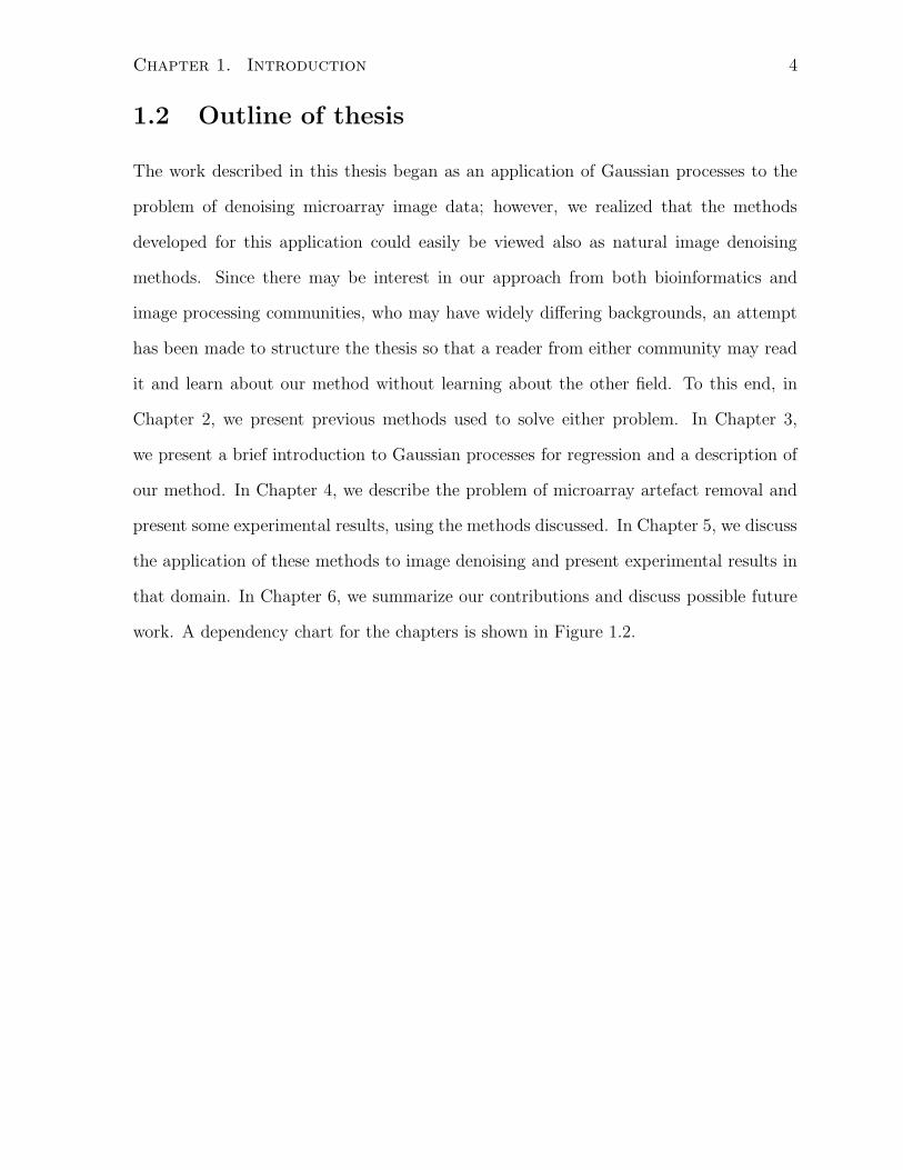
work. A dependency chart for the chapters is shown in Figure 1.2.
Chapter 1. Introduction 5
Chapter 1
Chapter 3
Chapter 2
Chapter 4 Chapter 5
Chapter 6
Figure 1.2: Chapter dependency chart.
Chapter 2
Related Work
The methods we will discuss in this section were designed for only one of image or mi-
croarray denoising applications, but may be used for either in principle. Before describing
related methods it is useful to have more definitions.
Recall our dataset D = {(xi, yi)}Ni=1 is in the form of a complete grid isomorphic
to a Euclidean rectangular plane, which for visualization purposes could be viewed as
an image. For simplicity, in this chapter we refer to each data point as a pixel and
pi = (xi, yi) as the ith pixel.
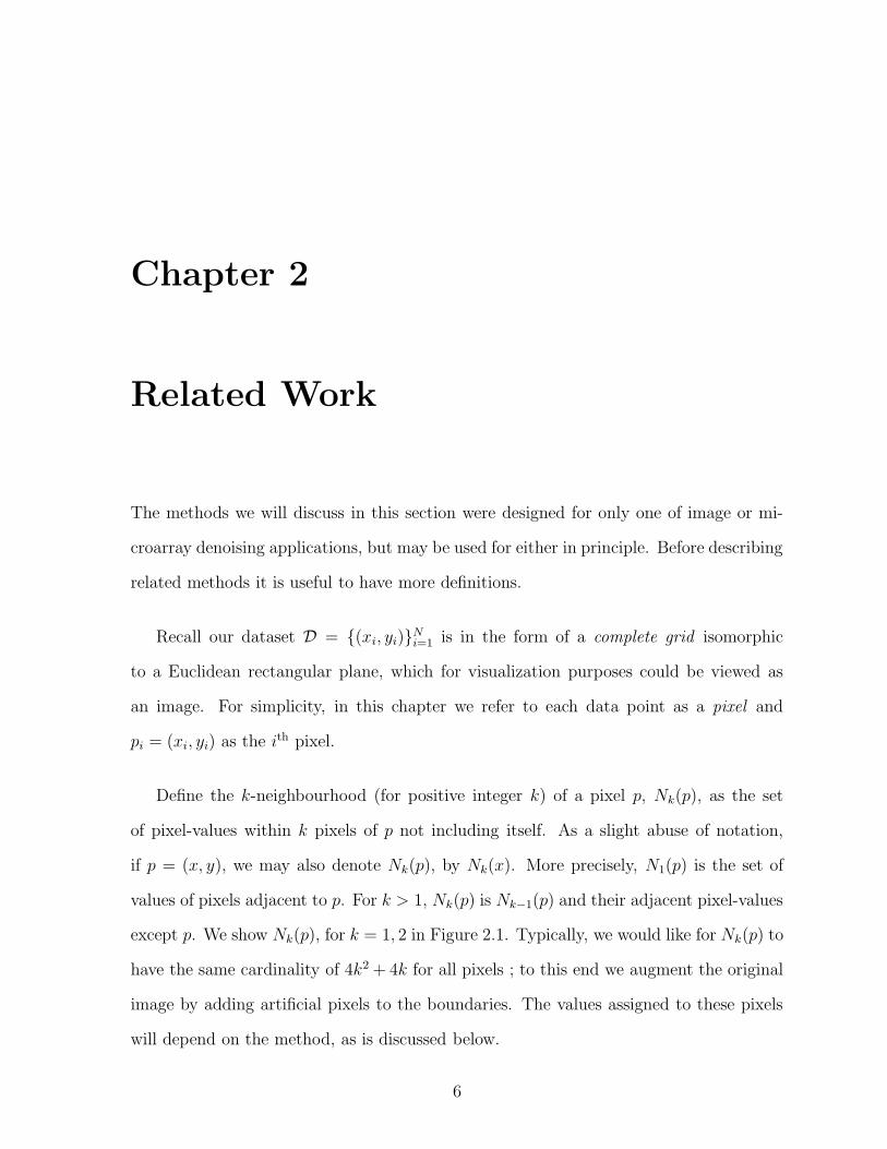
Define the k-neighbourhood (for positive integer k) of a pixel p, Nk(p), as the set
of pixel-values within k pixels of p not including itself. As a slight abuse of notation,
if p = (x, y), we may also denote Nk(p), by Nk(x). More precisely, N1(p) is the set of
values of pixels adjacent to p. For k > 1, Nk(p) is Nk−1(p) and their adjacent pixel-values
except p. We show Nk(p), for k = 1, 2 in Figure 2.1. Typically, we would like for Nk(p) to
have the same cardinality of 4k2 + 4k for all pixels ; to this end we augment the original
image by adding artificial pixels to the boundaries. The values assigned to these pixels
will depend on the method, as is discussed below.
6
Chapter 2. Related Work 7
p
(a) k = 1
p
(b) k = 2
Figure 2.1: k-neighbourhood pixels for pixel p are shown in gray.
2.1 Median filtering
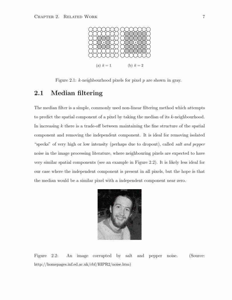
The median filter is a simple, commonly used non-linear filtering method which attempts
to predict the spatial component of a pixel by taking the median of its k-neighbourhood.
In increasing k there is a trade-off between maintaining the fine structure of the spatial
component and removing the independent component. It is ideal for removing isolated
“specks” of very high or low intensity (perhaps due to dropout), called salt and pepper
noise in the image processing literature, where neighbouring pixels are expected to have
very similar spatial components (see an example in Figure 2.2). It is likely less ideal for
our case where the independent component is present in all pixels, but the hope is that
the median would be a similar pixel with a independent component near zero.
Figure 2.2: An image corrupted by salt and pepper noise. (Source:
http://homepages.inf.ed.ac.uk/rbf/HIPR2/noise.htm)
Chapter 2. Related Work 8
2.2 Mean and Gaussian Filtering
For our problem, we can observe that E[yi] = E[si], and might aim to “average-out”
the zero-mean independent component by averaging the values of similar (defined by the
method) pixels. We will see that similarity effectively induces a set of weights {wij}Nj=1
to yield a weighted-average predictor (WAP) of the spatial component at pixel i, si =N∑
j=1
wijyj. The simplest such method is like the median filter except we take the mean
instead of the median. In our notation,
wij ∝
1, if yj ∈ Nk(xi)
0, otherwise(2.1)
N∑
j=1
wij = 1 (2.2)
In fact this coincides with nearest neighbours algorithm for grid data where the number
of neighbours is the size of the neighbourhood.
Gaussian filtering is a commonly used image filtering technique which is a WAP with
weights defined as
wij ∝ exp
(
−‖xi − xj‖22
h2
)
, i 6= j (2.3)
wii = 0 (2.4)
N∑
j=1
wij = 1 (2.5)
where ‖·‖2 is the L2 norm. Because of the rapid decay of wij as a function of the distance
‖xi − xj‖2, Gaussian smoothing is effectively a local filtering method.
The parameter h can be selected in a variety of ways. For example, the Spatial Trend
Removal (STR) method [9], which was developed to remove spatial trends in microarray
data, optimizes h using gradient-based optimization on the mean squared error between
the original and filtered datasets:
1
N
N∑
i=1
(yi − si)2 (2.6)
Chapter 2. Related Work 9
If viewed from a machine learning perspective, this error may be interpreted as the
leave-one-out cross-validation error in the task of predicting the original dataset.
In order to increase the smoothness of the estimated true image, STR ignores the
pixels which differ the most from an initial true image estimated by a median filter (7x7
window). The authors report that ignoring 10 % of pixels with the greatest difference
works well on their microarray data (this can be viewed as removing outliers). However,
this is an adjustable parameter.
As an image denoising algorithm, Gaussian filtering is well-known to over-smooth
images, resulting in the loss of significant detail, especially edge sharpness.
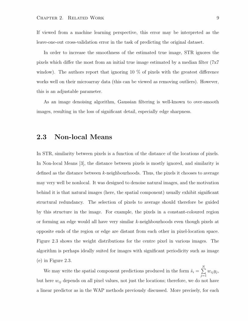
2.3 Non-local Means
In STR, similarity between pixels is a function of the distance of the locations of pixels.
In Non-local Means [3], the distance between pixels is mostly ignored, and similarity is
defined as the distance between k-neighbourhoods. Thus, the pixels it chooses to average
may very well be nonlocal. It was designed to denoise natural images, and the motivation
behind it is that natural images (here, the spatial component) usually exhibit significant
structural redundancy. The selection of pixels to average should therefore be guided
by this structure in the image. For example, the pixels in a constant-coloured region
or forming an edge would all have very similar k-neighbourhoods even though pixels at
opposite ends of the region or edge are distant from each other in pixel-location space.
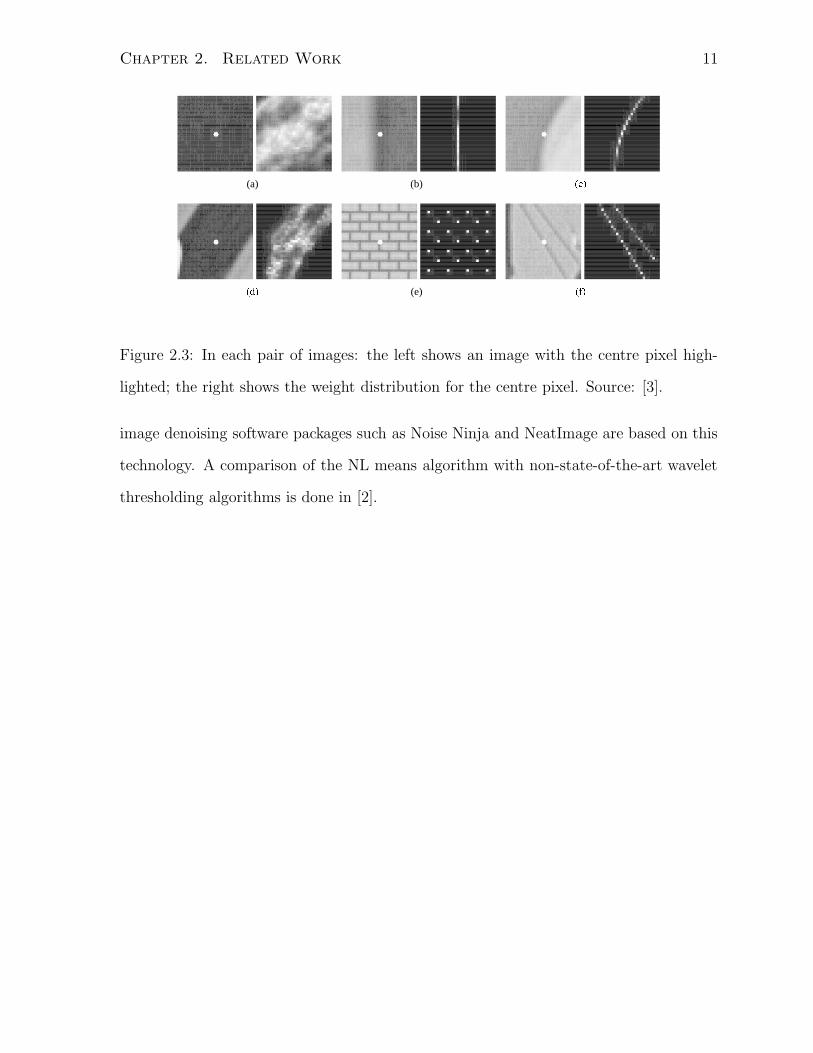
Figure 2.3 shows the weight distributions for the centre pixel in various images. The
algorithm is perhaps ideally suited for images with significant periodicity such as image
(e) in Figure 2.3.
We may write the spatial component predictions produced in the form si =N∑
j=1
wijyj,
but here wij depends on all pixel values, not just the locations; therefore, we do not have
a linear predictor as in the WAP methods previously discussed. More precisely, for each

Chapter 2. Related Work 10
pixel, p = (x, y), we may arbitrarily enumerate its k-neighbourhood, n1, . . . , n|Nk(x)|, and
form a neighbourhood-vector denoted, Vk(x) = (n1, . . . , n|Nk(x)|). Then we define the
weights as
wij ∝ exp
(
−‖Vk(xi) − Vk(xj)‖2
2,a
h2
)
, i 6= j (2.7)
wii = 0 (2.8)
N∑
j=1
wij = 1 (2.9)
where ‖·‖2,a is the weighted L2 norm, where the weights come from a Gaussian kernel
with variance a2.
The parameters to this algorithm are h and k. Although the authors of [3] do not
provide a methodology to choosing them, they suggest h ∈ [10σ, 15σ], where σ is an
estimate of the standard deviation of the independent component, and k = 7.
The time complexity is dominated by the pairwise neighbourhood-distance calcula-
tions O(kN 2). In practice, one might restrict attention to the pixels within a large
window centred on the pixel of interest to speed-up the algorithm and also force a local
bias in the weights. A new parameter M specifies the search window size. The time
for distance calculations is reduced to O(kNM 2) (note M2 ≤ N). The authors suggest
M = 21 works well in their experience.
2.4 Other methods not compared
There are a myriad other classes of methods which we do not review nor include in perfor-
mance comparisons in this thesis. Among them methods based on wavelet thresholding
([5]) from image processing are worth mentioning. Briefly, after performing a wavelet
transform, wavelet coefficients below a threshold (associated with high frequency noise)
are set to zero. These methods are fast, but it is unclear what the optimal set of wavelets
are. Although their algorithms are not open source, many state-of-the-art commercial
Chapter 2. Related Work 11
(a) (b) �����
����� (e) �����
Figure 2.3: In each pair of images: the left shows an image with the centre pixel high-
lighted; the right shows the weight distribution for the centre pixel. Source: [3].
image denoising software packages such as Noise Ninja and NeatImage are based on this
technology. A comparison of the NL means algorithm with non-state-of-the-art wavelet
thresholding algorithms is done in [2].

Chapter 3
Gaussian process method
3.1 Using Gaussian processes for noisy 2-dimensional
interpolation
Recall the decomposition of the observations into spatial and independent components
we are striving for
yi = si + ni (3.1)
In order for Gaussian processes to be used efficiently we assume {ni}Ni=1 are Gaussian
in addition to being independent, identically distributed with zero mean. We will see
that the variance of ni will be estimated from the data automatically.
Initially, we will also assume si = f(xi) for some unknown (latent) function of the
two coordinate inputs x; hence, ni will denote the departures of yi from f(xi) and our
task can be seen as determining the value of f at all data point locations, what one may
call the two-dimensional noisy interpolation problem.
The approach of parametric methods is to parameterize a class of functions conjec-
tured to contain the right f and use the data to estimate its parameters. Coming up with
the right parametric form is generally difficult. By contrast, Gaussian process regression
12
Chapter 3. Gaussian process method 13
discovers f without explicitly stating a parametric form but rather by vaguely specifying
its expected behaviour through a “distribution over functions”.
3.1.1 Gaussian process priors
A stochastic process is a collection of random variables {Yx : x ∈ I} indexed by some set
I, which often denotes time, but in general, as in our case, is multidimensional. Note
that x is not a random variable, but merely an index for random variables. We may
also write Yx as Y (x) to emphasize that x is typically viewed as the input and Y (x) as
the output (we use indices, inputs interchangeably). The Kolmogorov extension theorem
guarantees the existence of a stochastic process with consistent joint distributions for
any finite collection of random variables from the process [15]. Consistency here means
that the marginal probability distributions should agree with those derived from higher
dimensional joint distributions. Gaussian processes are stochastic processes where these
joint distributions are Gaussian.
A sample function of a stochastic process is a single realization of each of its random
variables. It can then be viewed as a function of the index set, I. For example, in our
case of grid data, the index set is a finite subset of a two-dimensional plane; hence, we
may visualize a sample function as a surface in R3. An interesting property of stochastic
processes is that the joint distributions defining it induce a distribution over sample
functions. In general, we do not know the analytic form of sample functions but, in
the case of Gaussian processes, can obtain the value of the function at an arbitrary
number of indices (inputs). We give a procedure for doing this in Section 3.1.2. With a
notion of “distribution over functions” in hand, we may talk about priors and posteriors
over functions induced by Gaussian processes. A distribution over functions can also
be achieved by parameterizing a class of functions and setting prior distributions over
the parameters, but the Gaussian process prior maybe preferred if no prior knowledge
justifies choosing a particular parametric form.
Chapter 3. Gaussian process method 14
The mean function, M : I → R, of a stochastic process specifies the mean of each
random variable M(x) = E[Yx]. The covariance function of a stochastic process, C :
I × I → R, specifies the covariance of any two random variables, C(x, x′) = Cov(Yx, Yx′)
and determines the smoothness properties of the process. As a Gaussian distribution is
completely specified by its mean and covariance, a mean function, M , and a covariance
function, C, completely specify a Gaussian process, which we denote GP(M, C).
If we have some strong prior knowledge of the behaviour of the mean function, we
could specify a parametric form – say of a quadratic polynomial M(x) = ax2 + bx + c
(with hyperparameters a, b, c) – but typically our knowledge is vague so we set M(x) to
a constant. By pre-processing our data we can make the most appropriate value for this
constant equal to zero.
Specifying the covariance function requires more thought, but as an illustration con-
sider the squared exponential covariance function:
C(x, x′) = σ2a exp
(
−∥
∥
∥
∥
x − x′
`
∥
∥
∥
∥
2)
(3.2)
where σ2a and ` are constants. The interpretation of these constants is elaborated in 3.1.4,
but we can immediately see that Cov(Yx, Yx′) is maximized when x and x′ are close,
encoding the prior belief that the sample functions from the corresponding Gaussian
process are continuous. In fact, with this covariance function they are differentiable [14],
which is not always a good assumption. If this were the only possible covariance function,
Gaussian process priors would be insufficiently expressive of our beliefs; luckily, there is
an infinite supply of covariance functions.
A real, symmetric function C on I × I is said to be semi-positive definite if for any
N , x1, . . . , xN ∈ I, and v ∈ RN , we have vTAv ≥ 0 where Aij = C(xi, xj). Given a semi-
positive definite function C, the Kolmogorov extension theorem guarantees that there
exists a (unique) zero-mean Gaussian process with covariance function E[y(x)y(x′)] =
C(x, x′) [20]. That is, there exists a zero-mean Gaussian process, GP(0, C), for every
Chapter 3. Gaussian process method 15
such “kernel” function, C. In practice most of the work in specifying a Gaussian process
prior is spent choosing the covariance function. This is the topic of Section 3.1.4.
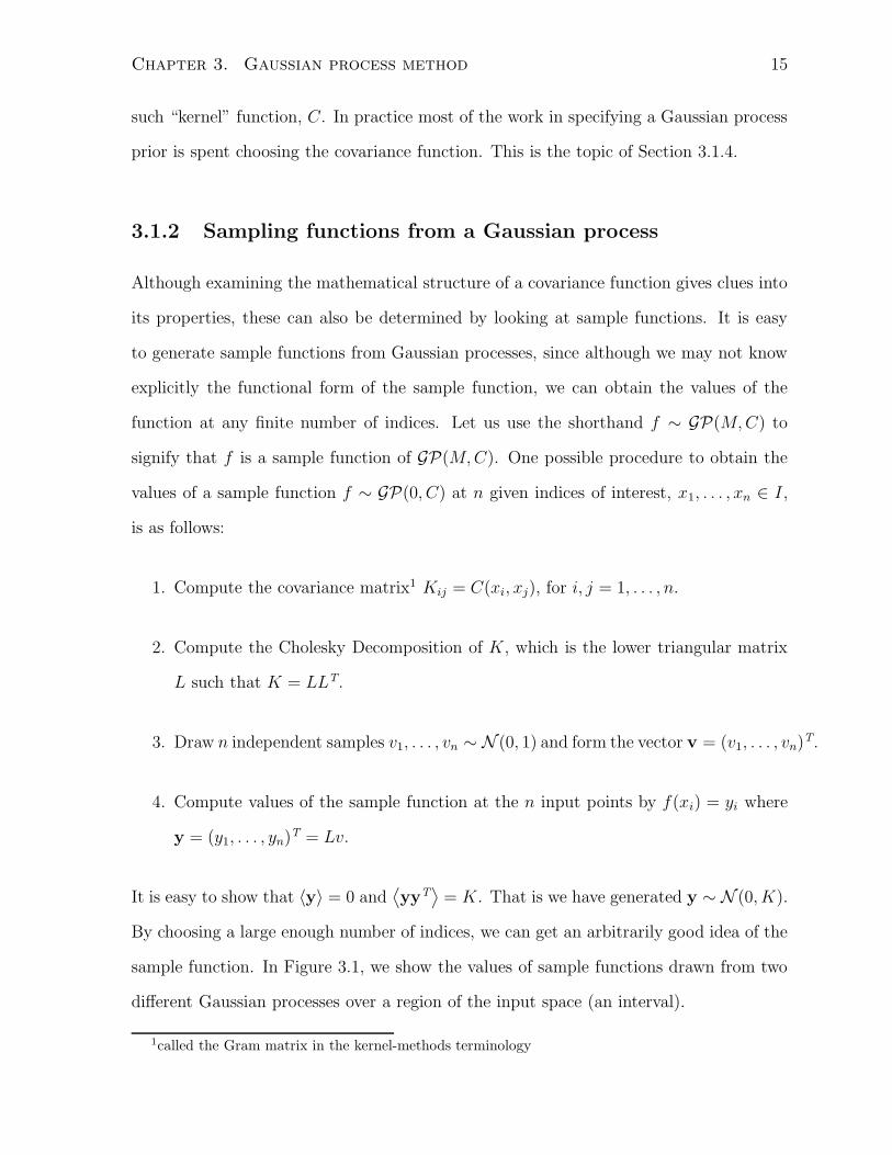
3.1.2 Sampling functions from a Gaussian process
Although examining the mathematical structure of a covariance function gives clues into
its properties, these can also be determined by looking at sample functions. It is easy
to generate sample functions from Gaussian processes, since although we may not know
explicitly the functional form of the sample function, we can obtain the values of the
function at any finite number of indices. Let us use the shorthand f ∼ GP(M, C) to
signify that f is a sample function of GP(M, C). One possible procedure to obtain the
values of a sample function f ∼ GP(0, C) at n given indices of interest, x1, . . . , xn ∈ I,
is as follows:
1. Compute the covariance matrix1 Kij = C(xi, xj), for i, j = 1, . . . , n.
2. Compute the Cholesky Decomposition of K, which is the lower triangular matrix
L such that K = LLT.
3. Draw n independent samples v1, . . . , vn ∼ N (0, 1) and form the vector v = (v1, . . . , vn)T.
4. Compute values of the sample function at the n input points by f(xi) = yi where
y = (y1, . . . , yn)T = Lv.
It is easy to show that 〈y〉 = 0 and⟨
yyT⟩
= K. That is we have generated y ∼ N (0, K).
By choosing a large enough number of indices, we can get an arbitrarily good idea of the
sample function. In Figure 3.1, we show the values of sample functions drawn from two
different Gaussian processes over a region of the input space (an interval).
1called the Gram matrix in the kernel-methods terminology
Chapter 3. Gaussian process method 16
−2 −1.5 −1 −0.5 0 0.5 1 1.5 2−2
−1.5
−1
−0.5
0
0.5
1
1.5
2
2.5
input, x
outp
ut, f
(x)
(a) squared exponential, ` = 1, σa = 1
−2 −1.5 −1 −0.5 0 0.5 1 1.5 2−3
−2
−1
0
1
2
3
input, x
outp
ut, f
(x)
(b) linear, ` = 1
Figure 3.1: 20 sample functions from zero-mean Gaussian Processes with squared-
exponential and linear (C(x, x′) = xTx′) covariance functions. Note that at each location,
x, the mean value over all functions is about zero.
3.1.3 Gaussian process regression
One possible way to approach the noisy interpolation problem is through Gaussian pro-
cess Regression (GPR). Although a form of GPR has long been practised by spatial
statisticians with a technique called kriging [4], renewed interest from the machine learn-
ing community began after it was re-derived in the Bayesian machine learning framework
and given a new probabilistic interpretation. Neal showed that the prior distribution en-
coded by certain neural networks converges to a Gaussian process in the limit of infinite
hidden units [11], and Rasmussen and Williams [21] investigated it as a general machine
learning method.
Suppose we want to have a prior “distribution” over functions without restricting
ourselves to a parametric form, and that we want to be able to compute a posterior over
functions having seen noisy data. GPR provides one way of doing so in a principled
(Bayesian) way. If we further assume a Gaussian noise model we can do this using
Chapter 3. Gaussian process method 17
efficient matrix operations. The noise model and prior over functions are
yi|f(xi) ∼ N (f(xi), σ2ε) (3.3)
f ∼ GP(0, C) (3.4)
where σ2ε) is the noise variance (to be estimated), and C is the covariance function of the
Gaussian process. The use of a zero-mean function for the Gaussian process encodes the
belief that at each location x, f(x) has equal probability of being positive or negative; it
does not say that sample functions themselves need have zero-mean. In order to make
this prior belief reasonable, we normalize the data to have (sample) mean of zero and
standard deviation of 1. We perform the same normalization to the inputs to simplify the
choice of initial hyperparameters when optimizing the marginal likelihood (see Section
3.1.5).
First, we consider the noise-less case, yi = f(xi). We learned how to sample functions
from the prior in the previous section, but really what we want to do in the context of
regression is to predict the values of f(x) for x not in the training data, i.e. test data. Let
us consider a single test input x∗ and predict its output y∗. Now the prior distribution
for y1, . . . , yn, y∗ is multivariate Gaussian, so the conditional distribution y∗|y1, . . . , yn is
univariate Gaussian. Some elementary manipulations using Gaussian identities yields
E[y∗|x∗, {(x, y)}Ni=1] = kTK−1[y1, . . . , yn]T (3.5)
V ar(y∗|x∗, {(x, y)}Ni=1) = Cov(x∗, x∗) − kTK−1k (3.6)
where k ∈ RN , ki = Cov(x∗, xi) (3.7)
We see that the mean is a linear combination of training outputs, which led spatial
statisticians to call it a linear predictor. The uncertainty in the value of the function
at the test input x∗ has been reduced, since kTK−1k ≥ 0, but the magnitude of this
reduction does not depend on the training outputs.
Chapter 3. Gaussian process method 18
One of the advantages of GPR is we have a full predictive distribution rather than
just a point prediction. If a point prediction is required we can determine the optimal
guess for our loss function from the predictive distribution; often we use the squared error
loss function, in which case we guess the mean of the distribution.
In the noise-free case, the predictive mean interpolates the training outputs exactly
and there is zero uncertainty (variance) in the output at the training inputs (for example
see figure 3.2). More realistically, we are interested in the case with noisy outputs:
y = f(x) + ε (3.8)
ε ∼ N (0, σ2ε) (3.9)
which we have seen before in equation 3.4. Conveniently, the additive noise assumption
means the covariance between outputs becomes
Cov(yi, yj) = C(xi, xj) + δijσ2ε (3.10)
where δij is 1 if i = j and 0 otherwise. That is, adding noise changes the covariance
function from C to (C + δσ2e). To obtain the covariance matrix, we simply add the diag-
onal matrix σ2εI to the old noise-free covariance matrix. We then can obtain analogous
predictive distribution equations for the noise-free output at x∗, denoted by f ∗:
E[f ∗|x∗, {(x, y)}Ni=1] = kT(K + σ2
εI)−1[y1, . . . , yn]T (3.11)
V ar(f ∗|x∗, {(x, y)}Ni=1) = Cov(x∗, x∗) − kT(K + σ2
εI)k (3.12)
where k ∈ RN , ki = Cov(x∗, xi) (3.13)
One notable difference between the noise-free and noisy cases, is that in the latter
case, the predictive mean of the noise-free outputs at the training input locations is in
general not equal to the training output (which has noise added). Indeed, we will use
the predictive mean as an estimate for the spatial component in the spatial-independent
decomposition in equation 3.1.

Chapter 3. Gaussian process method 19
−8 −6 −4 −2 0 2 4 6 8−3
−2
−1
0
1
2
3
input, x
outp
ut, f
(x)
(a) 10 samples functions from a GP prior
−8 −6 −4 −2 0 2 4 6 8−3
−2
−1
0
1
2
3
4
5
6
7
input, x
outp
ut, f
(x)
(b) Predictive distribution with noise-less ob-
servations
−8 −6 −4 −2 0 2 4 6 8−3
−2
−1
0
1
2
3
4
input, x
outp
ut, f
(x)
(c) Predictive distribution with noisy observa-
tions
Figure 3.2: Experiments with the squared exponential covariance function (` = 1, σa = 1,
σ2ε = 0.2). The predictive distributions are shown before and after seeing some data
points. The mean function is shown by the dark solid line; the two standard devia-
tion region at each location x is shown in gray. We see that in regions of sparse data,
the predictive distribution is unchanged from the prior and in data dense regions, the
uncertainty in the value of the latent function is smaller than in the prior.
Chapter 3. Gaussian process method 20
3.1.4 Selecting the covariance function
Since we assume a mean function equal to 0 (in the absence of knowledge), all we really
need to infer the latent function, f , is an appropriate covariance function that encodes
our prior beliefs of its behaviour. This is therefore where most of the tweaking/tuning
occurs in Gaussian process methods.
The approach we take is to decide on an appropriate class of covariance functions
indexed by hyperparameters (we call them hyperparameters since they parameterize our
prior for the latent function, not the latent function itself). We set these hyperparameters
to maximize an objective function called the evidence or marginal likelihood, which auto-
matically finds a compromise between model complexity and data fit. This is described
further in section 3.1.5.
Next, we describe a few common classes of covariance functions. Let D be the di-
mensionality of x.
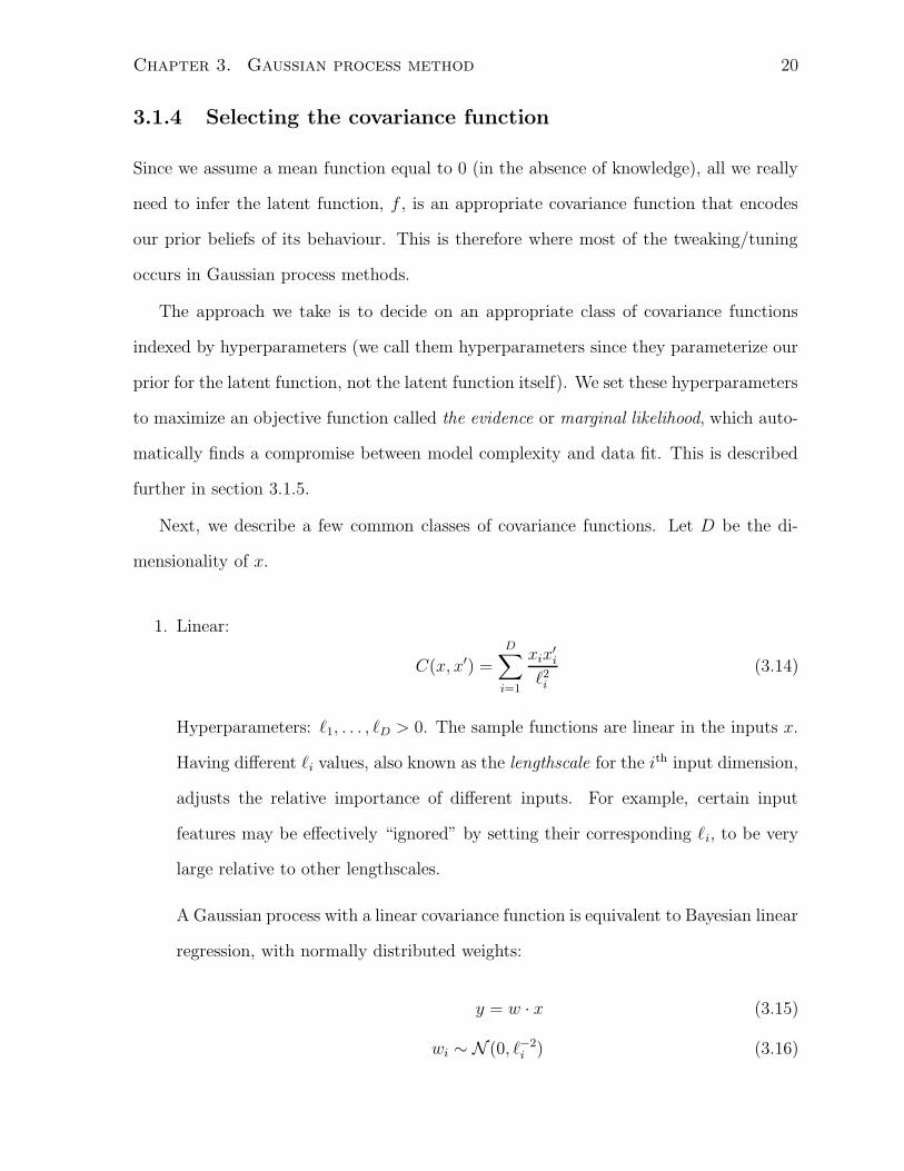
1. Linear:
C(x, x′) =D∑
i=1
xix′i
`2i
(3.14)
Hyperparameters: `1, . . . , `D > 0. The sample functions are linear in the inputs x.
Having different `i values, also known as the lengthscale for the ith input dimension,
adjusts the relative importance of different inputs. For example, certain input
features may be effectively “ignored” by setting their corresponding `i, to be very
large relative to other lengthscales.
A Gaussian process with a linear covariance function is equivalent to Bayesian linear
regression, with normally distributed weights:
y = w · x (3.15)
wi ∼ N (0, `−2i ) (3.16)
Chapter 3. Gaussian process method 21
Inferring w in this model is more efficient than the GP approach when D < N ,
since it involves inverting a D by D matrix rather than an N by N one. However,
it is useful to combine the linear term with another covariance function through
the operations of addition or multiplication to be discussed in the next section.
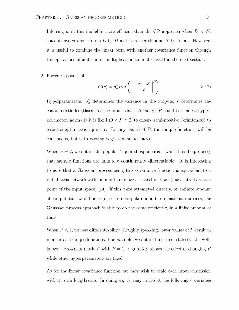
2. Power Exponential:
C(r) = σ2a exp
(
−∥
∥
∥
∥
x − x′
`
∥
∥
∥
∥
P)
(3.17)
Hyperparameters: σ2a determines the variance in the outputs; ` determines the
characteristic lengthscale of the input space. Although P could be made a hyper-
parameter, normally it is fixed (0 < P ≤ 2, to ensure semi-positive definiteness) to
ease the optimization process. For any choice of P , the sample functions will be
continuous, but with varying degrees of smoothness.
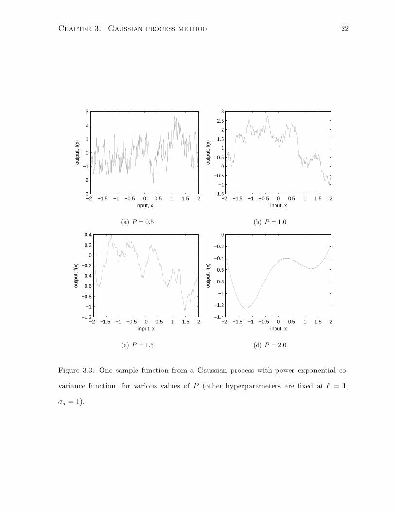
When P = 2, we obtain the popular “squared exponential” which has the property
that sample functions are infinitely continuously differentiable. It is interesting
to note that a Gaussian process using this covariance function is equivalent to a
radial basis network with an infinite number of basis functions (one centred on each
point of the input space) [14]. If this were attempted directly, an infinite amount
of computation would be required to manipulate infinite-dimensional matrices; the
Gaussian process approach is able to do the same efficiently, in a finite amount of
time.
When P < 2, we lose differentiability. Roughly speaking, lower values of P result in
more erratic sample functions. For example, we obtain functions related to the well-
known “Brownian motion” with P = 1. Figure 3.3, shows the effect of changing P
while other hyperparameters are fixed.
As for the linear covariance function, we may wish to scale each input dimension
with its own lengthscale. In doing so, we may arrive at the following covariance
Chapter 3. Gaussian process method 22
−2 −1.5 −1 −0.5 0 0.5 1 1.5 2−3
−2
−1
0
1
2
3
input, x
outp
ut, f
(x)
(a) P = 0.5
−2 −1.5 −1 −0.5 0 0.5 1 1.5 2−1.5
−1
−0.5
0
0.5
1
1.5
2
2.5
3
input, xou
tput
, f(x
)
(b) P = 1.0
−2 −1.5 −1 −0.5 0 0.5 1 1.5 2−1.2
−1
−0.8
−0.6
−0.4
−0.2
0
0.2
0.4
input, x
outp
ut, f
(x)
(c) P = 1.5
−2 −1.5 −1 −0.5 0 0.5 1 1.5 2−1.4
−1.2
−1
−0.8
−0.6
−0.4
−0.2
0
input, x
outp
ut, f
(x)
(d) P = 2.0
Figure 3.3: One sample function from a Gaussian process with power exponential co-
variance function, for various values of P (other hyperparameters are fixed at ` = 1,
σa = 1).
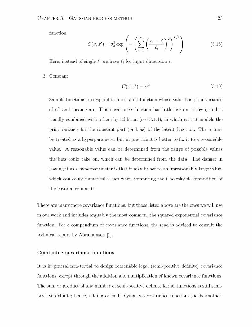
Chapter 3. Gaussian process method 23
function:
C(x, x′) = σ2a exp
−(
D∑
i=1
(
xi − x′i
`i
)2)P/2
(3.18)
Here, instead of single `, we have `i for input dimension i.
3. Constant:
C(x, x′) = α2 (3.19)
Sample functions correspond to a constant function whose value has prior variance
of α2 and mean zero. This covariance function has little use on its own, and is
usually combined with others by addition (see 3.1.4), in which case it models the
prior variance for the constant part (or bias) of the latent function. The α may
be treated as a hyperparameter but in practice it is better to fix it to a reasonable
value. A reasonable value can be determined from the range of possible values
the bias could take on, which can be determined from the data. The danger in
leaving it as a hyperparameter is that it may be set to an unreasonably large value,
which can cause numerical issues when computing the Cholesky decomposition of
the covariance matrix.
There are many more covariance functions, but those listed above are the ones we will use
in our work and includes arguably the most common, the squared exponential covariance
function. For a compendium of covariance functions, the read is advised to consult the
technical report by Abrahamsen [1].
Combining covariance functions
It is in general non-trivial to design reasonable legal (semi-positive definite) covariance
functions, except through the addition and multiplication of known covariance functions.
The sum or product of any number of semi-positive definite kernel functions is still semi-
positive definite; hence, adding or multiplying two covariance functions yields another.
Chapter 3. Gaussian process method 24
Thus,
Cadd(x, x′) = C1(x, x′) + C2(x, x′) (3.20)
Cprod(x, x′) = C1(x, x′) · C2(x, x′) (3.21)
are valid covariance functions, if C1 and C2 are too.
Sample functions drawn from a GP with covariance Cadd exhibit the properties of
functions drawn separately from C1 and C2 and then added. The interpretation of the
product operation is less obvious but we may observe that while in the case of addition,
a large contribution from either C1 or C2 will result in a large overall covariance, in
the case of product, both C1 and C2 need to be large for the overall covariance to be
large. Another way to make use of these combination operations is to have C1 and C2
depend on different subsets of the inputs; in fact, we take this approach in section 3.2.
As can be imagined, a great variety of covariance functions can be produced through
these operations based on small set of base covariance functions.
Other ways of combining covariance functions into new ones are discussed in [17].
3.1.5 Selecting hyperparameters
Bayesian approach
In the Bayesian formalism, all parameters and hyperparameters have prior distributions
encoding our beliefs. Because Gaussian process regression is a non-parametric method,
we only have to worry about hyperparameters, which we denote by θC (having fixed
our covariance function C). The predictive distribution for a new test output yN+1
(given dataset, D = {(xi, yi)}Ni=1) is obtained by averaging predictions from different
hyperparameters weighted by their posterior probability:
p(yN+1|xN+1,D) =
∫
p(yN+1|xN+1,D, θC)p(θC |xN+1,D)dθC (3.22)
In general, equation 3.22 cannot be evaluated analytically, and we need to resort to
numerical methods. The investigation of these methods is beyond the scope of this thesis;

Chapter 3. Gaussian process method 25
for a full treatment see the work of Neal ([12],[10]), and Rasmussen and Williams [14].
One property of these methods is that they require significant additional computation
time, which we avoid in order to maximize the practicality of our algorithm.
Marginal likelihood / evidence maximization
Instead of averaging predictions from all hyperparameter sets, as an approximation we
may use the prediction from the single set with maximum posterior probability, given by
p(θC |D) ∝ p(y| {x}Ni=1 , θC)p(θC) (3.23)
where y = (y1, . . . , yN), p(y| {x}Ni=1 , θC) is the probability of the data or (the evidence,
or marginal likelihood) and p(θC) is the prior distribution on the hyperparameters. For
simplicity, this prior is often ignored (i.e. set to improper uniform), although using a
proper prior may help rule out unreasonable values of θC ; therefore, maximization of the
posterior probability of the hyperparameters reduces to maximization of the evidence.
The maximization problem is non-convex in general and it is carried out through a
gradient-based optimization technique such as conjugate-gradients, or L-BFGS. Numer-
ically, it is easier to perform this maximization in the log domain. Since we know that
y| {xi}Ni=1 , θ ∼ N (0, K), we have
log(p(y| {xi}Ni=1 , θ)) = −N
2log(2π) − 1
2log(|K|) − 1
2yTK−1y (3.24)
from which we can obtain the gradient with respect to θ
∂ log(p(y| {xi}Ni=1 , θ))
∂θ= −1
2tr(K−1∂K
∂θ) +
1
2yTK−1∂K
∂θK−1y (3.25)
The asymptotic time complexity is dominated by the inversion of K, the covariance
matrix, which takes O(N 3) time. As with all non-convex optimization problems, local
optima can be a problem, although perhaps not too serious a one in practice, since the
number of hyperparameters is usually small relative to the number of data points [8].
Chapter 3. Gaussian process method 26
In our experiments, we have chosen to use the approach of evidence maximization
rather than the true Bayesian approach, in order to make the algorithm more practical
in terms of time complexity and avoiding the difficulty of choosing appropriate prior
distributions for hyperparameters.
3.1.6 Limitations of the 2-d interpolation approach
Except for the linear covariance function, the basic covariance functions we discussed
all can be written as a function of the separation vector x − x′, between two inputs x
and x′. Covariance functions that have this property are called stationary. It is readily
seen that the operations of addition and multiplication of covariance functions preserve
stationarity. Unfortunately, stationarity implies certain reasonable functions are highly
improbable such as functions which vary rapidly in one part of the input space and slowly
in another. This corresponds to a process with a input-dependent (i.e. non-stationary)
lengthscale. A concrete 1-dimensional example of this is shown in figure 3.4, where a
rapid change in the function only occurs at two isolated parts of the input space and is
unchanging elsewhere.
Although the linear covariance function is non-stationary, it only has the power to add
a linear trend to sample functions. Dealing with reasonable non-stationary covariance
functions is somewhat involved and beyond the scope of this thesis, but it is examined
in the work of Paciorek [13]. In the next section, we propose a novel way to extend the
modelling power of stationary covariance functions in the special case of grid data.
3.2 Adding pseudo-inputs to grid data
Recall that in two-dimensional grid data, the data points are uniformly spaced in a
rectangle. Each point has a k-neighbourhood as defined in Chapter 2 (boundary cases
are treated specially). Our aim is to incorporate local neighbourhood information into the

Chapter 3. Gaussian process method 27
−10 −8 −6 −4 −2 0 2 4 6 8 10−3
−2
−1
0
1
2
3
4
5
6
input
outp
ut
(a) latent function
−10 −8 −6 −4 −2 0 2 4 6 8 10−3
−2
−1
0
1
2
3
4
5
6
input
outp
ut(b) GP squared exponential, large lengthscale
−10 −8 −6 −4 −2 0 2 4 6 8 10−2
−1
0
1
2
3
4
5
6
input
outp
ut
(c) GP squared exponential, short lengthscale
Figure 3.4: A function that is badly modelled by stationary Gaussian processes. We
added a small amount of noise, sampled a few data points, then modelled it with a
squared exponential GP. We show the predictive distributions of two different sets of
parameters corresponding to different local maxima in the marginal likelihood. In (b)
the predictive model is too simple; in (c) it is too complex.
Chapter 3. Gaussian process method 28
Gaussian process previously discussed for 2-dimensional noisy interpolation, effectively
making the covariance vary throughout the grid even if the distance between points is
fixed while still using a stationary covariance function. We achieve this by adding extra
inputs to the data points.
Previously our input x was simply the two Cartesian coordinates encoding the location
of our data points. Let us now call this xcoord, and consider augmenting our input vector
with neighbourhood information, xneigh = Vk(xcoord) (we find k = 1 works best) 2, and
define our new, augmented input vector, xaug = (xcoord, xneigh). It is perhaps incorrect to
call xneigh extra inputs since they correspond to the noisy outputs for other data points;
for this reason we use the term pseudo-inputs for xneigh. However, in the following we
treat them as if they were regular inputs.
The covariance function we use to combine the two input sets in a reasonable way is:
C(xaug, x′aug) = σ2
aCcoord(xcoord, x′coord)Cneigh(xneigh, x
′neigh) (3.26)
Ccoord(xaug, x′aug) = exp
(
−|xcoord − x′coord|2
l2coord
)
(3.27)
Cneigh(xaug, x′aug) = exp
(
−∣
∣xneigh − x′neigh
∣
∣
2
l2neigh
)
(3.28)
or
C(xaug, x′aug) = σ2
a exp
(
−|xcoord − x′coord|2
l2coord
−∣
∣xneigh − x′neigh
∣
∣
2
l2neigh
)
(3.29)
There are two characteristic length-scales, one for the location and one for the neigh-
bourhood. This allows the model to automatically determine which of the two “super
features” of distance in actual space and distance in neighbourhood space is more rele-
vant. Fixing lcoord and letting lneigh → ∞, we get the 2-d interpolation scheme introduced
in section 3.1; while fixing lneigh and letting lcoord → ∞ we get a covariance only depend-
ing on neighbourhood as in the NL-means algorithm. Having these as hyperparameters
2Recall the definition from Chapter 2: Vk(x) is the set of k-neighbourhood values centred at x, putin a vector.

Chapter 3. Gaussian process method 29
allows for the evidence maximization mechanism to decide how to trade-off between the
two extremes of using mostly local and mostly non-local information to calculate the
covariance between outputs.
The resulting covariance function encodes our prior belief that data points both near
each other and with similar neighbourhood structures should have similar outputs. Al-
though the covariance functions used are all stationary, the predictions produced clearly
cannot come from a stationary process depending on only location inputs.
One consequence of using a higher-dimensional input space is we have lost continuity
with respect to xcoord, i.e. two data points which are close in the grid may be far apart
in the new input space, therefore freeing the outputs from being close. However, if the
locations and the neighbourhoods of two data points are close (which is not uncommon,
e.g. a constant region), the covariance will be large and the outputs close. This behaviour
is actually desirable and preferable in our situation since the type of surfaces we wish to
model are not globally continuous. For example, consider modelling an edge in a natural
image. Points on either side of the edge are close in location but have unrelated outputs
(discontinuous), whereas points on the edge have similar outputs (continuous). As pre-
viously mentioned in section 2.3, the points on the edge have similar k-neighbourhoods,
different from those on either side of the edge. In our augmented input space this subtlety
can be learned by the model.
We have also lost the ability to generate datasets, since our pseudo-inputs require
knowning the dataset beforehand! However, given a noisy dataset, we can generate
the noise-free (or spatial) component corresponding to the dataset, which is where our
interest primarily lies.
3.2.1 Novel general algorithm for denoising grid data
Our algorithm for discovering the decomposition of noisy grid data is to use GPR with a
zero-mean function and a covariance function which is a sum of covariance functions we
Chapter 3. Gaussian process method 30
have discussed:
C(x, x′) = α + C1(x, x′) + δ(x, x′)σ2ε (3.30)
C1(x, x′) = σ2a exp
(
−|xcoord − x′coord|2
l2coord
−∣
∣xneigh − x′neigh
∣
∣
2
l2neigh
)
(3.31)
The hyperparameters of the covariance function are σa, lcoord, lneigh, σε, and α. Usually
α can be set manually based on the data (see 3.1.4) but the rest are learned (in the
absence of other knowledge) by maximizing the evidence. It suffices to initialize the
hyperparameters to reasonable values.
After the hyperparameters are selected, the mean of the predictive distribution at
each grid location is used as the prediction for the spatial component. The difference of
this and the actual value is the prediction for the independent component.
For large grids, it may be better to have different sets of hyperparameters for different
regions of the grid. We consider a scheme for achieving this in the next section.
3.3 Managing the O(N 3) time complexity
The space complexity of Gaussian process Regression is only O(N 2), required to store
the covariance matrix, so it is mainly the O(N 3) time complexity which poses a problem.
For modern computers, datasets larger than 104 are infeasible and limiting N to 103 or
less is desirable.
We overcome this difficulty by partitioning the grid into fixed-sized, overlapping
patches and running our algorithm on each patch separately. By fixing the size of a
patch to Npart pixels, the time complexity is now O(N 3partP ), where P is the number of
patches. Since the number of patches grows linearly with the number of pixels, asymp-
totically our algorithm is now linear in the number of pixels, O(N), with a constant
factor corresponding to the time to process a single patch.
The partitioning scheme also adds flexibility to the model by allowing the hyperpa-
rameters of our covariance function to be different in different patches. This allows our

Chapter 3. Gaussian process method 31
method to better model widely differing features throughout the image. The patch size
should be small enough so that the GP model can explain the within-patch variability,
but not too small so as not to have enough data points for learning / pattern discovery.
A partitioning of the standard “Lena” image which works well is found in figure 3.5. The
patches are made to overlap so as to increase the continuity of the predictions when mov-
ing between patches. Predictions in the overlapping regions are calculated by averaging
the predictions from individual patches.
Our approach of partitioning the space is similar to splines, where, say, a cubic poly-
nomial may not be able capture the underlying function well, but may approximate it
well in a small interval; the use of multiple cubic polynomials with different parameters
in each partition of space is analogous to what we do. Often, splines are constrained to
be continuous at the knots (boundaries of partitions), but we don’t explicitly force this.
In chapter 4, we also investigate reducing the dataset by summarizing blocks of data by
(a) Lena image (b) with partitions
Figure 3.5: A possible partitioning of the standard 512x512 image of “Lena”. The patches
are mostly 29x29 in size.
their median and then using the block medians as data values.
Chapter 3. Gaussian process method 32
3.4 Details of marginal likelihood optimization step
In our implementation, we normalize the inputs and outputs to have mean 0 and variance
1 in a pre-processing step. Initially, we initialize the hyperparameters σa, lcoord, lneigh = 1
and initialize σ2ε to an estimate of the independent-component variance. We fix α = 36
rather than leave it as a hyperparameter. The hyperparameter search is carried out
using conjugate-gradients as a first-order gradient-based method when maximizing the
marginal likelihood. With this initialization, we obtained consistently good local maxima,
making additional random restarts unnecessary.
Processing a single 30 x 30 patch in our MATLAB implementation takes approxi-
mately 4 minutes with a 3 GHz CPU.
Chapter 4
Microarray denoising
Our first application of the methods discussed is for removing spatial artefacts in data
from DNA microarray experiments. Readers interested only in the domain of image
de-noising may skip this chapter and move on to the next one without loss of continuity.
4.1 Description of the problem
Often biologists or medical researchers are interested in the relative expression levels
of segments of deoxyribonucleic acid (DNA) – usually genes – in various experimental
conditions (e.g. brain/liver tissue). By expression we mean the process through which
DNA is “transcribed” to produce RNA, which may serve a regulatory purpose in the
cell or be “translated” into a protein in the case of genes. A common way of measuring
the expression level is to measure the abundance of a product of transcription, the RNA
transcript. Even in the case in which transcription of DNA does not result in a protein,
the RNA transcript abundance is still of interest as it may serve a regulatory role in the
cell.
A common tool used to measure the abundance of RNA in a cell is the DNA mi-
croarray. A sensor with thousands of spots or probes, each designed to bind to some
33
Chapter 4. Microarray denoising 34
sequence of bases from the set A,C,G,T1. The probes are arranged in a uniformly spaced
two-dimensional grid, or array. Microarrays can be constructed economically and rapidly
and allow parallel, high-throughput generation of data. Typically, the spacing between
probes is small, allowing for thousands of probes to be placed on a glass slide (also a
called microarray chip) roughly the size of a finger tip.
In a process called hybridization, a (tissue) sample of interest is dyed with a fluo-
rophore then washed onto the slide to allow binding. In the imaging step, a laser is
shone on the array, causing the dye to fluoresce. The amount of fluorescence at each spot
is related to the amount of binding and in turn to the RNA abundance in the sample.
From each spot, the imaging software derives an intensity value. These values are then
normalized [18].
In practice it is possible to hybridize two differently dyed (using Cy3 or Cy5) samples
to a single microarray. In spotted microarrays, this technique may be used to measure
the relative expression levels in control and patient samples; in oligonucleuotide arrays
(e.g. the data we discuss in this chapter), the signals are of sufficiently high quality that
it is possible to measure the absolute abundance of RNA for two samples at each spot.
For more details on the technology of microarrays, the reader may consult Schena’s book
([16]).
By design, the order in which the probes are placed on the microarray slide is usually
randomized (certainly in the dataset we use); hence, we expect very little correlation
between position and expression after hybridization. This assumption is crucial to our
denoising approach since the presence of spatial structure in the expression data can
then be attributed to spatial artefact noise which arises from imperfect experimental
procedures. There is a multitude of noise sources which we do not attempt to exhaustively
examine, but they may include
1Adenosine (A), Guanine (G), Thymine (T), Cytonsine (C) – the four nucleic acids of DNA and thebuilding blocks of the genetic code
Chapter 4. Microarray denoising 35
• stray dust particles on the slide or imaging lens [18];
• touching of the slide with fingers or other objects
• non-uniform “washing” in the hybridization process,
In other words, a great many possible things can contribute spatial artefacts and it is
imprudent to place many restrictions on the shapes of artefacts we expect. Instead, we
assume that the diversity of shapes is similar to that found in natural images, which tend
to have a significant amount of continuity, along with some sharp edges.
There are other sources of noise in microarray data, such as that produced by cross-
hybridization, in which probes bind to the wrong segment of DNA [7], but we ignore
these.
4.2 Data used in our experiments
We test our methods on mouse gene expression microarray data created by Zhang et al.
[23] for gene function prediction. The microarrays they use are of the oligonucleotide
variety, allowing for two different simultaneous hybridizations in the Cy3 and Cy5 chan-
nels in a process called fluor reversal. The result is we have two microarray images
per slide (which we will call green and red), but we treat the data as if it were created
from two separate slides. Conveniently, the dataset contains replicates (one from each
channel, green and red) for each experiment; i.e. for each microarray experiment, there
are two hybridizations on different slides. We take advantage of these replicates in our
performance metric, as discussed in Section 4.4.
There are N = 21939 spots arranged in a 213-by-103 grid. Henceforth, the direction
along the longer length will be called the vertical direction and the other will be called
the horizontal direction.
We informally observed that there is a large diversity of spatial artefact shapes across
Chapter 4. Microarray denoising 36
all slides, but not so much within a slide. This observation (along with preliminary
experiments) influenced our decision to use only two partitions (see 3.3) for each slide.
Remember, having finer partitions allows us to have more sets of hyperparameters in our
Gaussian process tailored to different parts of the slide. The second reason for having
finer partitions is that it reduces the computational complexity of processing the entire
slide; however, we address this aspect by learning the hyperparameters on a reduced
dataset, described in the next section.
4.3 GP algorithm for microarray artefact removal
Our approach to microarray denoising is to model the (log of the) intensity at each probe
as the sum of spatially-independent and spatially-dependent components, seen as the
contributions from the true expression level of the probe and the microarray’s spatial
artefacts, respectively. The spatial artefact component is also called the local/spatial
trend or background, and its removal is called detrending. Once the background over the
entire slide has been estimated, it can be removed by subtraction. In our algorithm, the
spatial trend is a latent function inferred using Gaussian process regression and the true
expression levels are modelled by IID Gaussian noise2. The covariance function we use
was described in Section 3.2.1.
The Gaussian model for the expression levels is not quite appropriate, since the actual
distribution has a heavy right tail [9]. To make the data more amenable to our model,
we derive a new dataset where the outputs are the medians of 3x3 non-overlapping
blocks from the grid data, and the inputs are the centre (two) coordinates of the block
and the 1-neighbourhood of the block, which is defined as the values of the data points
directly adjacent to the block but not part of the block. Note that the 1-neighbourhood
of a data point corresponds to the 1-neighbourhood of a block of size 1x1. Figure 4.1
2Note that the data is positive. As mentioned in Chapter 3, to make a zero-mean gaussian processreasonable, we pre-process the data so that it has zero mean
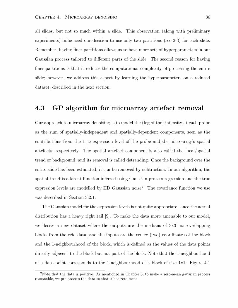
Chapter 4. Microarray denoising 37
shows a 3x3 block centred at a point p along with its 1-neighbourhood. The hope in
p
Figure 4.1: Shows the 1-neighbourhood of a 3x3 block centred at p. The gray coloured
circles are part of the 3x3 block and the black coloured circles form the 1-neighbourhood
of the block. The white circles are other grid data points.
this pre-processing step is that the spatial artefacts over a 3x3 block are approximately
constant, and hence removing the extreme data values from consideration by taking
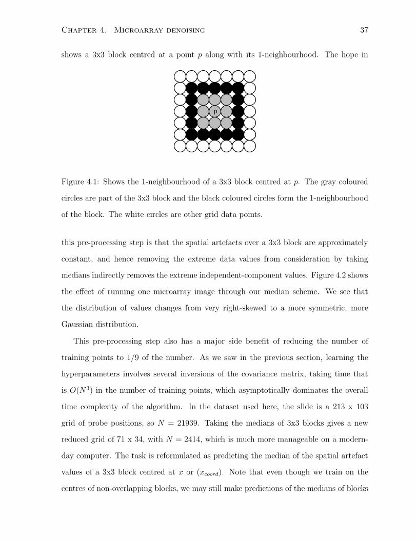
medians indirectly removes the extreme independent-component values. Figure 4.2 shows
the effect of running one microarray image through our median scheme. We see that
the distribution of values changes from very right-skewed to a more symmetric, more
Gaussian distribution.
This pre-processing step also has a major side benefit of reducing the number of
training points to 1/9 of the number. As we saw in the previous section, learning the
hyperparameters involves several inversions of the covariance matrix, taking time that
is O(N3) in the number of training points, which asymptotically dominates the overall
time complexity of the algorithm. In the dataset used here, the slide is a 213 x 103
grid of probe positions, so N = 21939. Taking the medians of 3x3 blocks gives a new
reduced grid of 71 x 34, with N = 2414, which is much more manageable on a modern-
day computer. The task is reformulated as predicting the median of the spatial artefact
values of a 3x3 block centred at x or (xcoord). Note that even though we train on the
centres of non-overlapping blocks, we may still make predictions of the medians of blocks
Chapter 4. Microarray denoising 38
3 4 5 6 7 8 9 10 11 120
200
400
600
800
1000
1200
3.5 4 4.5 5 5.5 6 6.5 7 7.5 80
10
20
30
40
50
60
70
80
90
Figure 4.2: Top: A microarray slide (log domain) and its histogram of values. Bottom:
The derived median version and its histogram of values.
Chapter 4. Microarray denoising 39
centred at all 21939 (test) locations on the slide. This step is linear in the number of test
points once the covariance matrix is inverted (taking time O(N 3) in the training points).
In representing the original microarray image with 1/9 as much data, there is obvi-
ously a loss in resolution resulting in the loss of some fine spatial artefacts (say a 1 pixel
line). However, such fine artefact structure is rare and the overall effect of ignoring it is
small when using the correlation performance metric described in the next section.
Our medians-scheme is by no means the only way to increase the Gaussianity of data.
Snelson et al. ([19] ) investigates learning the parameters of a data transformation from
a class (which includes log-like functions) simultaneously with the hyperparameters of
the covariance function. In their Gaussian smoothing algorithm, Shai et al. ([9]) ignore
data points whose values exceed a certain departure from a preliminary estimate of the
local trend. However, only our scheme reduces the data set size while increasing its
Gaussianity.
In our MATLAB implementation, processing each of the two partitions per chip takes
approximately 4 minutes on a 3 GHz CPU computer.
4.4 Experimental methodology
We compare our own Gaussian Process method (“GP”) with Gaussian filtering / smooth-
ing (“STR”, see 2.2), and a median filter with a 1-neighbourhood (“Medians”, see 2.1).
We do not compare with the NL-means algorithm since according to its developers, the
choice of h (controls degree of filtering, see 2.3) should depend on the standard deviation
of the independent component, σε, which is unknown here. We attempted to estimate
it by looking at the average (absolute) difference between adjacent values divided by
two, but found that this was only accurate when the independent-component was small
compared to the dependent-component, which is not the case in microarray data.
The performance metric we will use is the increase in correlation between the two
Chapter 4. Microarray denoising 40
replicates of a microarray experiment after processing by the algorithm:
ρ(Ngreen, Nred) − ρ(Ygreen, Yred) (4.1)
where Ygreen, Yred are the original green and red microarray image data, respectively,
and Ngreen, Nred are the estimates of their independent parts made by the algorithm
whose performance we are measuring, and ρ is the sample correlation between two sets
of measurements. It is important to emphasize that the algorithms process each replicate
independently, and do not depend on the existence of replicates; the replicate information
is used here only to measure performance. In general, replicates are not expected for the
algorithms we discuss.
This metric is more appropriate for our purposes than mean squared error since a
ground truth is unavailable, but we have replicates; furthermore, we are not concerned
with the actual values of the expression, just the relative values within the slide. Under
perfect experimental conditions, we expect the correlation to be very close to 1; in reality,
this often is not the case. An ideal microarray denoising algorithm would bring the
correlation between the two replicates as close to 1 as possible without destroying the
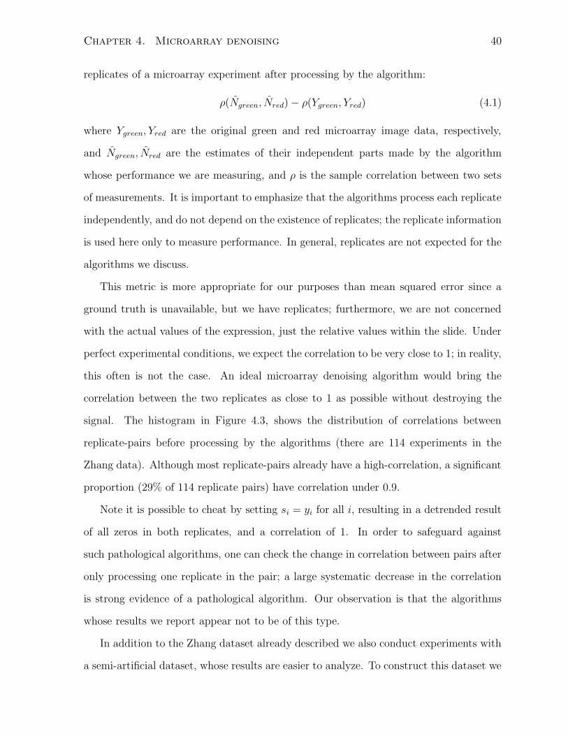
signal. The histogram in Figure 4.3, shows the distribution of correlations between
replicate-pairs before processing by the algorithms (there are 114 experiments in the
Zhang data). Although most replicate-pairs already have a high-correlation, a significant
proportion (29% of 114 replicate pairs) have correlation under 0.9.
Note it is possible to cheat by setting si = yi for all i, resulting in a detrended result
of all zeros in both replicates, and a correlation of 1. In order to safeguard against
such pathological algorithms, one can check the change in correlation between pairs after
only processing one replicate in the pair; a large systematic decrease in the correlation
is strong evidence of a pathological algorithm. Our observation is that the algorithms
whose results we report appear not to be of this type.
In addition to the Zhang dataset already described we also conduct experiments with
a semi-artificial dataset, whose results are easier to analyze. To construct this dataset we
Chapter 4. Microarray denoising 41
0 0.1 0.2 0.3 0.4 0.5 0.6 0.7 0.8 0.9 10
5
10
15
20
25
30
35
40
45
50Distribution of pre−processed chip−pair correlations
correlation
num
ber
of c
hips
Figure 4.3: histogram of correlations between replicate pair experiments
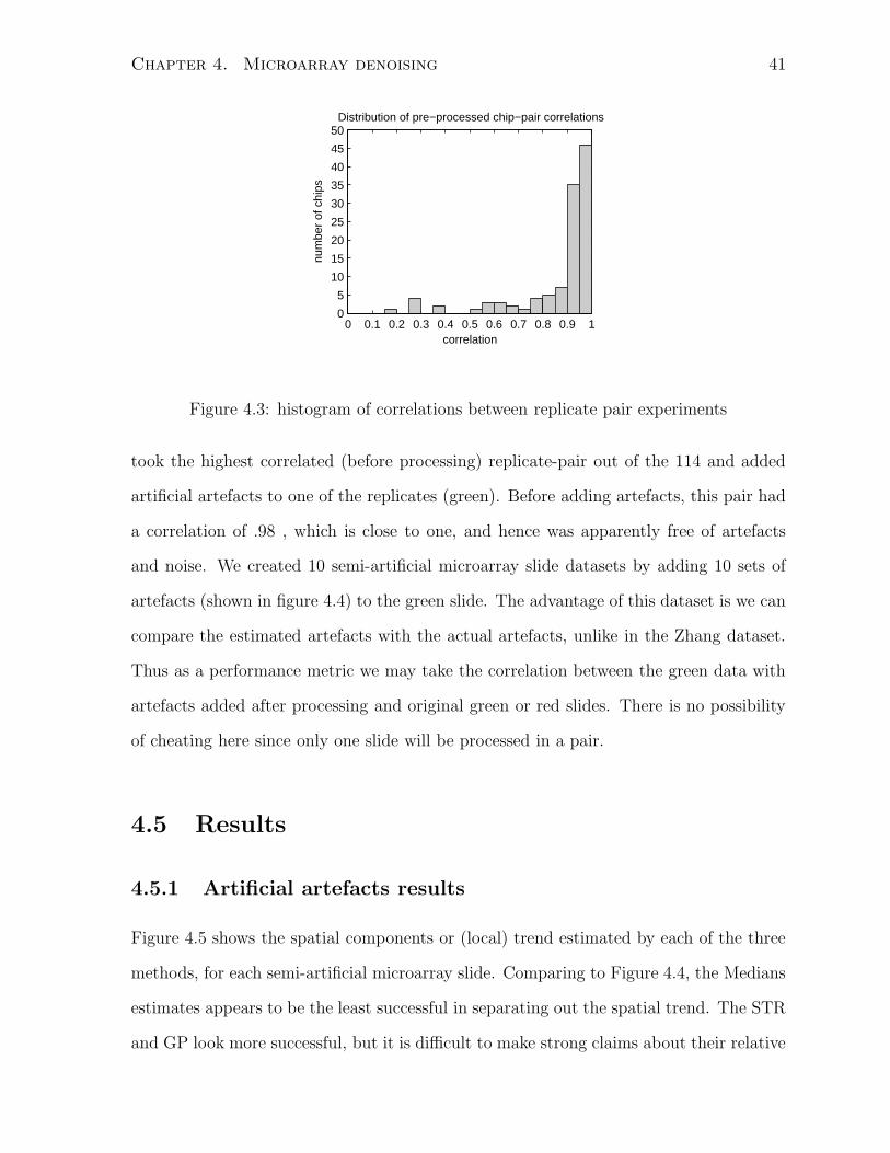
took the highest correlated (before processing) replicate-pair out of the 114 and added
artificial artefacts to one of the replicates (green). Before adding artefacts, this pair had
a correlation of .98 , which is close to one, and hence was apparently free of artefacts
and noise. We created 10 semi-artificial microarray slide datasets by adding 10 sets of
artefacts (shown in figure 4.4) to the green slide. The advantage of this dataset is we can
compare the estimated artefacts with the actual artefacts, unlike in the Zhang dataset.
Thus as a performance metric we may take the correlation between the green data with
artefacts added after processing and original green or red slides. There is no possibility
of cheating here since only one slide will be processed in a pair.
4.5 Results
4.5.1 Artificial artefacts results
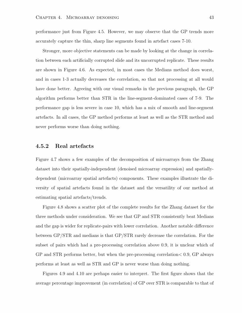
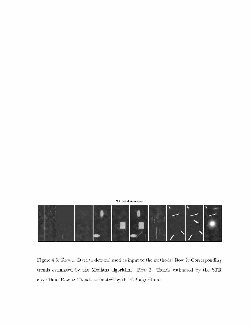
Figure 4.5 shows the spatial components or (local) trend estimated by each of the three
methods, for each semi-artificial microarray slide. Comparing to Figure 4.4, the Medians
estimates appears to be the least successful in separating out the spatial trend. The STR
and GP look more successful, but it is difficult to make strong claims about their relative
Chapter 4. Microarray denoising 42
Artefacts
0.5
1
1.5
2
2.5
3
original green
4 4.5 5 5.5 6 6.5 7
original green + Art 10
4 4.5 5 5.5 6 6.5 7
Figure 4.4: Top row: Ten sets of artificial artefacts (we label them 1,. . . , 10 from left to
right) to be added to a microarray data slide. Bottom row: the original slide to which
artefacts are added and the result of adding the 10th set of artefacts
Chapter 4. Microarray denoising 43
performance just from Figure 4.5. However, we may observe that the GP trends more
accurately capture the thin, sharp line segments found in artefact cases 7-10.
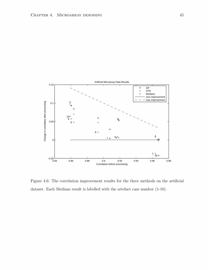
Stronger, more objective statements can be made by looking at the change in correla-
tion between each artificially corrupted slide and its uncorrupted replicate. These results
are shown in Figure 4.6. As expected, in most cases the Medians method does worst,
and in cases 1-3 actually decreases the correlation, so that not processing at all would
have done better. Agreeing with our visual remarks in the previous paragraph, the GP
algorithm performs better than STR in the line-segment-dominated cases of 7-9. The
performance gap is less severe in case 10, which has a mix of smooth and line-segment
artefacts. In all cases, the GP method performs at least as well as the STR method and
never performs worse than doing nothing.
4.5.2 Real artefacts
Figure 4.7 shows a few examples of the decomposition of microarrays from the Zhang
dataset into their spatially-independent (denoised microarray expression) and spatially-
dependent (microarray spatial artefacts) components. These examples illustrate the di-
versity of spatial artefacts found in the dataset and the versatility of our method at
estimating spatial artefacts/trends.
Figure 4.8 shows a scatter plot of the complete results for the Zhang dataset for the
three methods under consideration. We see that GP and STR consistently beat Medians
and the gap is wider for replicate-pairs with lower correlation. Another notable difference
between GP/STR and medians is that GP/STR rarely decrease the correlation. For the
subset of pairs which had a pre-processing correlation above 0.9, it is unclear which of
GP and STR performs better, but when the pre-processing correlation< 0.9, GP always
performs at least as well as STR and GP is never worse than doing nothing.
Figures 4.9 and 4.10 are perhaps easier to interpret. The first figure shows that the
average percentage improvement (in correlation) of GP over STR is comparable to that of
Chapter 4. Microarray denoising 44
Artefacts plus green data
Medians trend estimates
STR trend estimates
GP trend estimates
Figure 4.5: Row 1: Data to detrend used as input to the methods. Row 2: Corresponding
trends estimated by the Medians algorithm. Row 3: Trends estimated by the STR
algorithm. Row 4: Trends estimated by the GP algorithm.
Chapter 4. Microarray denoising 45
0.84 0.86 0.88 0.9 0.92 0.94 0.96 0.98−0.05
0
0.05
0.1
0.15
1 2 3
4 5
6
7
8
9
10
Correlation before processing
Cha
nge
in c
orre
latio
n af
ter
proc
essi
ng
Artificial Microarray Data Results
GPSTRMedianszero improvementmax improvement
Figure 4.6: The correlation improvement results for the three methods on the artificial
dataset. Each Medians result is labelled with the artefact case number (1-10).
Chapter 4. Microarray denoising 46
STR over medians and the magnitude of this improvement increases as the pre-processing
correlation decreases. The second figure shows a similar result using negative percentage
change in 1-correlation as a measure of improvement.
4.6 Discussion
We have shown that our GP algorithm performs at least as well as and often better than
STR in both our semi-artificial and the real, Zhang dataset on low PPC replicate-pairs.
In the real data case, the percentage improvement of GP over STR is comparable to that
of STR over medians.
With Gaussian process regression methods, one has to be careful with the time com-
plexity, but our median-scheme combined with partitioning each slide into two has made
the total processing time per chip comparable to STR3– on the order of 10 minutes with
a 3 GHz CPU (doing each partition sequentially). Our algorithm can scale linearly to
larger microarrays by fixing the partition size while increasing the number of partitions.
Median filtering is still much faster but its performance is likely unacceptable.
3In the STR algorithm, determining the Gaussian kernel parameter by gradient-based optimizationdominates the time complexity.

Chapter 4. Microarray denoising 47
Figure 4.7: Eight examples of microarray decompositions by the our method into spatial
and independent components. In each triplet of images, the left one is the original
microarray slide, the centre is the estimated spatial component, and the right is the
estimated independent component.

Chapter 4. Microarray denoising 48
0.2 0.3 0.4 0.5 0.6 0.7 0.8 0.9
0
0.1
0.2
0.3
0.4
0.5
Correlation before processing
Cha
nge
in c
orre
latio
n af
ter
proc
essi
ng
Zhang Microarray Data Results
GPSTRmedianszero improvementmax improvement
0.9 0.91 0.92 0.93 0.94 0.95 0.96 0.97 0.98−0.02
−0.01
0
0.01
0.02
0.03
0.04
0.05
0.06
0.07
Correlation before processing
Cha
nge
in c
orre
latio
n af
ter
proc
essi
ng
Zhang Microarray Data Results (subset)
Figure 4.8: Top: Scatter plot of improvement results for all replicate pairs in the Zhang
dataset. Bottom: Improvement results for replicate pairs with pre-processing correlation
of at least 0.9.
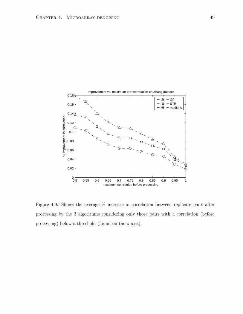
Chapter 4. Microarray denoising 49
0.5 0.55 0.6 0.65 0.7 0.75 0.8 0.85 0.9 0.95 10
0.02
0.04
0.06
0.08
0.1
0.12
0.14
0.16
0.18
maximum correlation before processing
% im
prov
emen
t in
corr
elat
ion
Improvement vs. maximum pre−correlation on Zhang dataset
GPSTRmedians
Figure 4.9: Shows the average % increase in correlation between replicate pairs after
processing by the 3 algorithms considering only those pairs with a correlation (before
processing) below a threshold (found on the x-axis).
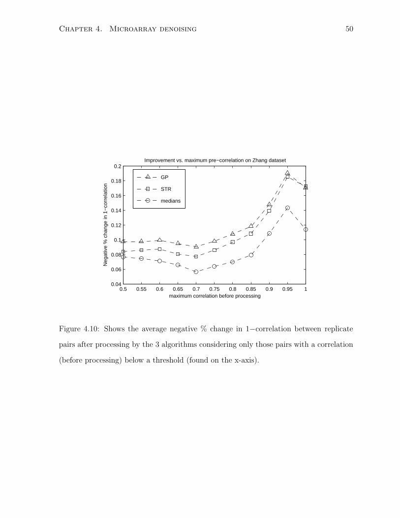
Chapter 4. Microarray denoising 50
0.5 0.55 0.6 0.65 0.7 0.75 0.8 0.85 0.9 0.95 10.04
0.06
0.08
0.1
0.12
0.14
0.16
0.18
0.2
maximum correlation before processing
Neg
ativ
e %
cha
nge
in 1
−co
rrel
atio
n
Improvement vs. maximum pre−correlation on Zhang dataset
GP
STR
medians
Figure 4.10: Shows the average negative % change in 1−correlation between replicate
pairs after processing by the 3 algorithms considering only those pairs with a correlation
(before processing) below a threshold (found on the x-axis).
Chapter 5
Image denoising
5.1 Description of Problem
Images captured by digital cameras or scanners are rarely noise-free. The nature of the
noise artefacts in images can vary significantly, but here we focus on the unavoidable
shot noise of the charge-coupled device (CCD), the main image sensor in most imaging
devices. The CCD is essentially a two-dimensional array partitioned into small, equal-
sized, (usually) square regions called pixels, each of which has sensors designed to estimate
the number of photons arriving in its region in some time interval (exposure time). In
the extreme cases of low-light or fast-action photography, the number of photons is small
enough that the sampling error is detrimental; in most other cases, the effect is not
as noticeable but still undesirable. The random process of photon counting is usually
thought to be a Poisson process, where we expect the number of photons, P , to have
standard deviation√
P [2]; that is, the noise is intensity dependent. However, as a
simplification, most noise models in the image processing literature assume the noise is
independent, identically distributed (IID) Gaussian. When the mean number of photons
is huge, the Poisson distribution is well-approximated by a Gaussian.
Usually image data is received in the form of a matrix specifying the grey-level or
51
Chapter 5. Image denoising 52
RGB vector for a pixel in row i and column j. Without loss of generality1, we restrict
ourselves to grey-level images; after re-labelling the data and allowing x to be the (row,
column) of a pixel and y to be the grey-level of the image, we see we have two-dimensional
grid data {(xi, yi)}Ni=1 ⊂ R
2 × R. If we let the true image be the spatial component and
the shot noise be the independent component, we arrive at the decomposition problem
discussed in Chapter 1.
5.2 GP algorithm for denoising images
Our image denoising algorithm first divides an arbitrary natural image into approximately
30x30 pixel patches, which overlap with adjacent patches by 6 pixels on all sides (see
3.3). For each patch, we use Gaussian process regression using the covariance function
described in Equation 3.31 to obtain the predictive mean of the noise-free image, which
in this case is the spatial component. Once predictions are obtained for each patch, we
combine them to produce the complete denoised image. Multiple predictions at the same
pixel are averaged.
Recall, that in our covariance function, the hyperparameter σ2ε controls the estimate
of the variance in the independent component (IID Gaussian). This can be learned along
with the other hyperparameters, or can be fixed to an estimate obtained from the user.
In commercial image denoising software, the estimate is often obtained with the aid of the
user, who provides a bounding box around a region of the image with no detail. In our
experiments, we assume this estimate is available and fix σ2ε accordingly. This increases
the robustness of the hyperparameter learning by avoiding certain bad local maxima in
the marginal likelihood.
1to denoise a colour image, denoise the R,G, and B channels separately
Chapter 5. Image denoising 53
5.3 Experimental methodology
To compare image denoising algorithms, we will take three relatively noise-free images,
add various amounts of IID Gaussian noise artificially, attempt to remove the noise using
the algorithms, and compare the denoised results with the original images.
5.3.1 Adding artificial noise to images
Let σ2image be the sample variance of an image before adding noise. Define the signal-to-
noise ratio (SNR) of the image with artificially added white noise N(0, σ2noise) as
σimage/σnoise (5.1)
A lower SNR corresponds to a noisier image, or in our earlier terminology, an image with
a larger independent component contribution to each pixel. In practice, an image with
SNR of 10 has barely noticeable noise, and one with an SNR of less than 2 is unacceptable
to most people. For our experiments, we add noise such that the SNR is 2, 5, and 10
(identical noise patterns, but different noise magnitudes).
5.3.2 Performance metrics
We focus on two algorithm performance metrics. One is quantitative and objective, the
other is qualitative and subjective, but perhaps more natural.
Because we are adding noise ourselves to a ground truth image, we can calculate the
mean squared error (MSE) between the denoised image and true image:
1
N
N∑
i=1
(si − si)2 (5.2)
where si is the true value of the ith pixel, and si is its estimated value from the noisy
data. This error measure has the advantage of being objective and is often used in the
image processing literature to compare algorithms.

Chapter 5. Image denoising 54
The other performance metric is simply a visual comparison of true and denoised
images by people. We present these results by showing the actual images and discussing
their visual qualities. An attempt will be made to make only obvious statements, which
the reader presumably will find non-controversial.
In certain pathological cases, the MSE metric and human-visual metric produce very
different rankings. A simple example is an algorithm which perfectly denoises an image
and translates it 1 pixel to the left. Calculating only the MSE would lead one to believe
that the algorithm is very bad; whereas, most humans would not notice the translation
and believe the algorithm is very good based only on visual inspection. Apart from
such cases, we find that the MSE metric often agrees with visual inspection, but visual
inspection can offer insight unobtainable from just the MSE numbers.
5.3.3 Image data
We use three commonly used images in the image denoising literature. Lena, Barbara
and Boat.2 The three images are shown in Figure 5.1. Each image is a 512x512 pixel,
8-bit graylevel image exhibiting a large range of intensity and detail. The Lena image
has a mix of very low detail in the skin and the background with very high detail in the
hat. The Barbara image has less extreme range of detail but also has periodic properties
in the tablecloth and head covering. The Boat image has a very high amount of detail
throughout most of the image, except in some regions of the sky.
5.3.4 Methods selected for comparison
As baselines in the MSE results, we use median filtering (“medians”) with a 1-neighbourhood
(see Section 2.1), and Gaussian filtering using STR (see Section 2.2) without outlier de-
2Grayscale Lena obtained by averaging RGB channels of color version found at
http://www.cs.cmu.edu/∼chuck/lennapg/lenna.shtml. Barbara and Boat images obtainedfrom http://decsai.ugr.es/∼javier/denoise/test images/index.htm.

Chapter 5. Image denoising 55
(a) Lena (b) Barbara
(c) Boat
Figure 5.1: The original images before adding noise.
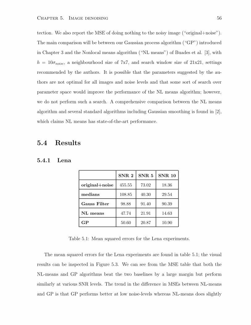
Chapter 5. Image denoising 56
tection. We also report the MSE of doing nothing to the noisy image (“original+noise”).
The main comparison will be between our Gaussian process algorithm (“GP”) introduced
in Chapter 3 and the Nonlocal means algorithm (“NL means”) of Buades et al. [3], with
h = 10σnoise, a neighbourhood size of 7x7, and search window size of 21x21, settings
recommended by the authors. It is possible that the parameters suggested by the au-
thors are not optimal for all images and noise levels and that some sort of search over
parameter space would improve the performance of the NL means algorithm; however,
we do not perform such a search. A comprehensive comparison between the NL means
algorithm and several standard algorithms including Gaussian smoothing is found in [2],
which claims NL means has state-of-the-art performance.
5.4 Results
5.4.1 Lena
SNR 2 SNR 5 SNR 10
original+noise 455.55 73.02 18.36
medians 108.85 40.30 29.54
Gauss Filter 98.88 91.40 90.39
NL means 47.74 21.91 14.63
GP 50.60 20.87 10.90
Table 5.1: Mean squared errors for the Lena experiments.
The mean squared errors for the Lena experiments are found in table 5.1; the visual
results can be inspected in Figure 5.3. We can see from the MSE table that both the
NL-means and GP algorithms beat the two baselines by a large margin but perform
similarly at various SNR levels. The trend in the difference in MSEs between NL-means
and GP is that GP performs better at low noise-levels whereas NL-means does slightly
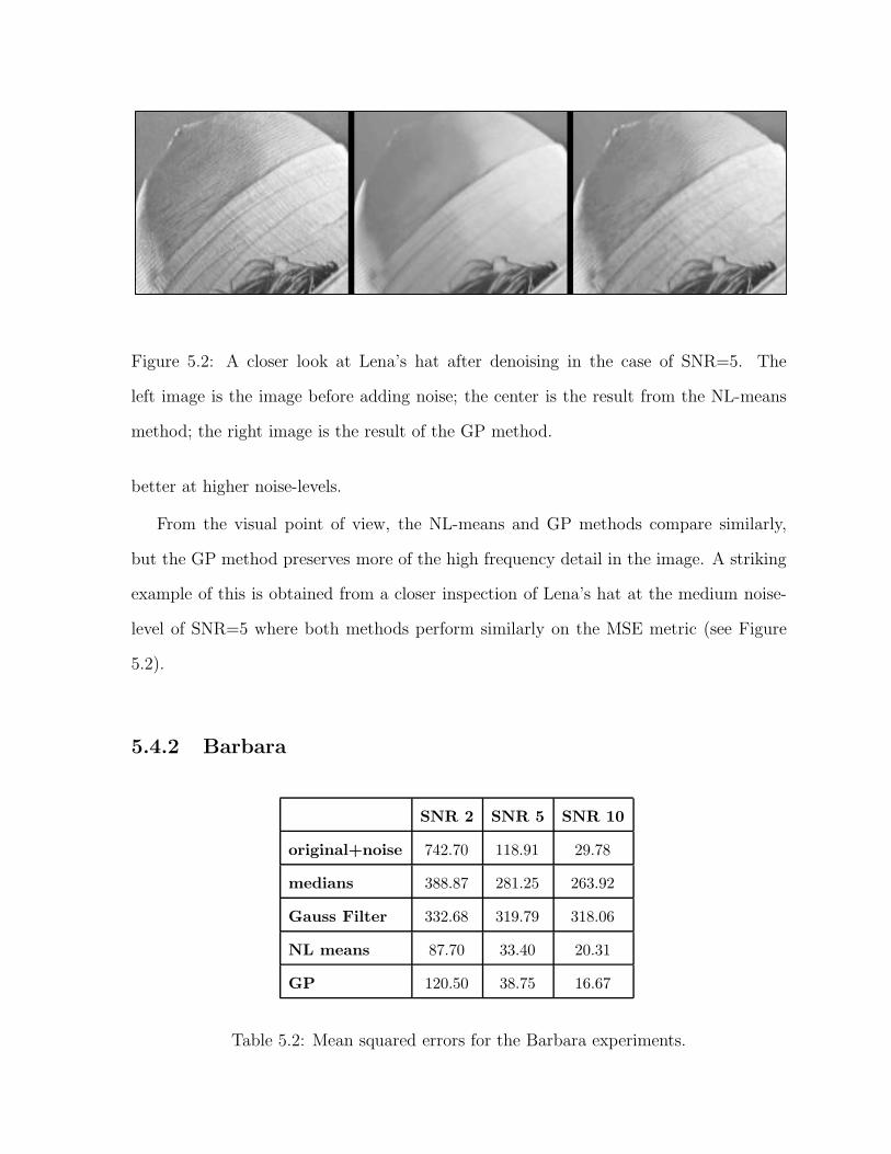
Chapter 5. Image denoising 57
Figure 5.2: A closer look at Lena’s hat after denoising in the case of SNR=5. The
left image is the image before adding noise; the center is the result from the NL-means
method; the right image is the result of the GP method.
better at higher noise-levels.
From the visual point of view, the NL-means and GP methods compare similarly,
but the GP method preserves more of the high frequency detail in the image. A striking
example of this is obtained from a closer inspection of Lena’s hat at the medium noise-
level of SNR=5 where both methods perform similarly on the MSE metric (see Figure
5.2).
5.4.2 Barbara
SNR 2 SNR 5 SNR 10
original+noise 742.70 118.91 29.78
medians 388.87 281.25 263.92
Gauss Filter 332.68 319.79 318.06
NL means 87.70 33.40 20.31
GP 120.50 38.75 16.67
Table 5.2: Mean squared errors for the Barbara experiments.
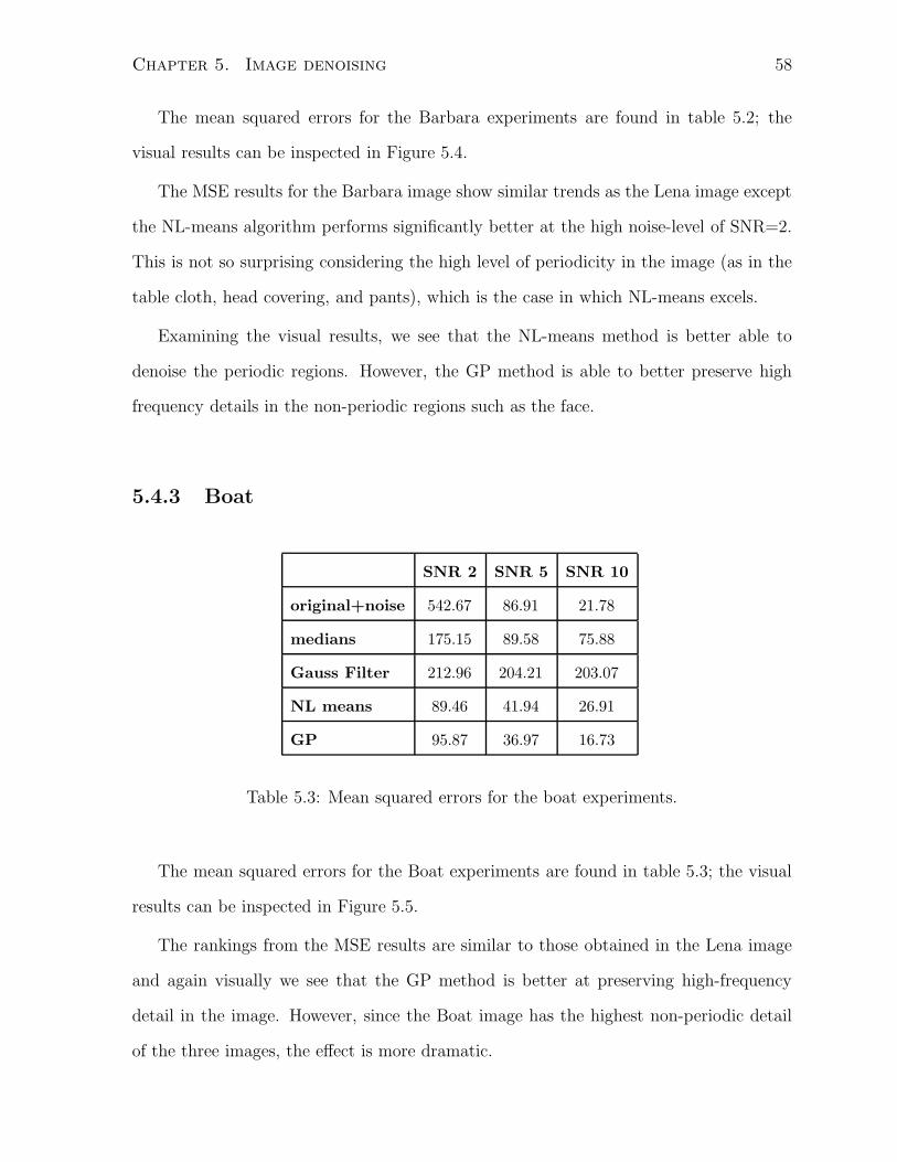
Chapter 5. Image denoising 58
The mean squared errors for the Barbara experiments are found in table 5.2; the
visual results can be inspected in Figure 5.4.
The MSE results for the Barbara image show similar trends as the Lena image except
the NL-means algorithm performs significantly better at the high noise-level of SNR=2.
This is not so surprising considering the high level of periodicity in the image (as in the
table cloth, head covering, and pants), which is the case in which NL-means excels.
Examining the visual results, we see that the NL-means method is better able to
denoise the periodic regions. However, the GP method is able to better preserve high
frequency details in the non-periodic regions such as the face.
5.4.3 Boat
SNR 2 SNR 5 SNR 10
original+noise 542.67 86.91 21.78
medians 175.15 89.58 75.88
Gauss Filter 212.96 204.21 203.07
NL means 89.46 41.94 26.91
GP 95.87 36.97 16.73
Table 5.3: Mean squared errors for the boat experiments.
The mean squared errors for the Boat experiments are found in table 5.3; the visual
results can be inspected in Figure 5.5.
The rankings from the MSE results are similar to those obtained in the Lena image
and again visually we see that the GP method is better at preserving high-frequency
detail in the image. However, since the Boat image has the highest non-periodic detail
of the three images, the effect is more dramatic.
Chapter 5. Image denoising 59
5.5 Discussion
We have shown our GP method performs favourably – especially at moderate to low noise
levels – against the NL-means algorithm, using the program settings recommended by the
authors in [3]. We make this claim with respect to both the MSE and visual inspection
(the ultimate) performance metrics. However, we note that in the visual results we saw
that the GP method is significantly better at preserving non-periodic, high-frequency
detail.
Since most real applications of image denoising occur at the medium-to-low noise
levels, our GP method is likely better than the other methods in most practical situations.
Although our algorithm scales linearly in the number of pixels when the patch (par-
tition) size is fixed, the time taken for each patch (30x30 pixel) partition is on the order
of 5 minutes. For the test images used, this translated to a total time for denoising an
image on the order of several hours in a MATLAB implementation run on a 3 GHz CPU
doing one patch at a time, whereas a good implementation of NL-means would take a few
minutes. Although, the time complexity of our method is within the limits of feasibility,
future work in accelerating our method would increase its general usefulness.
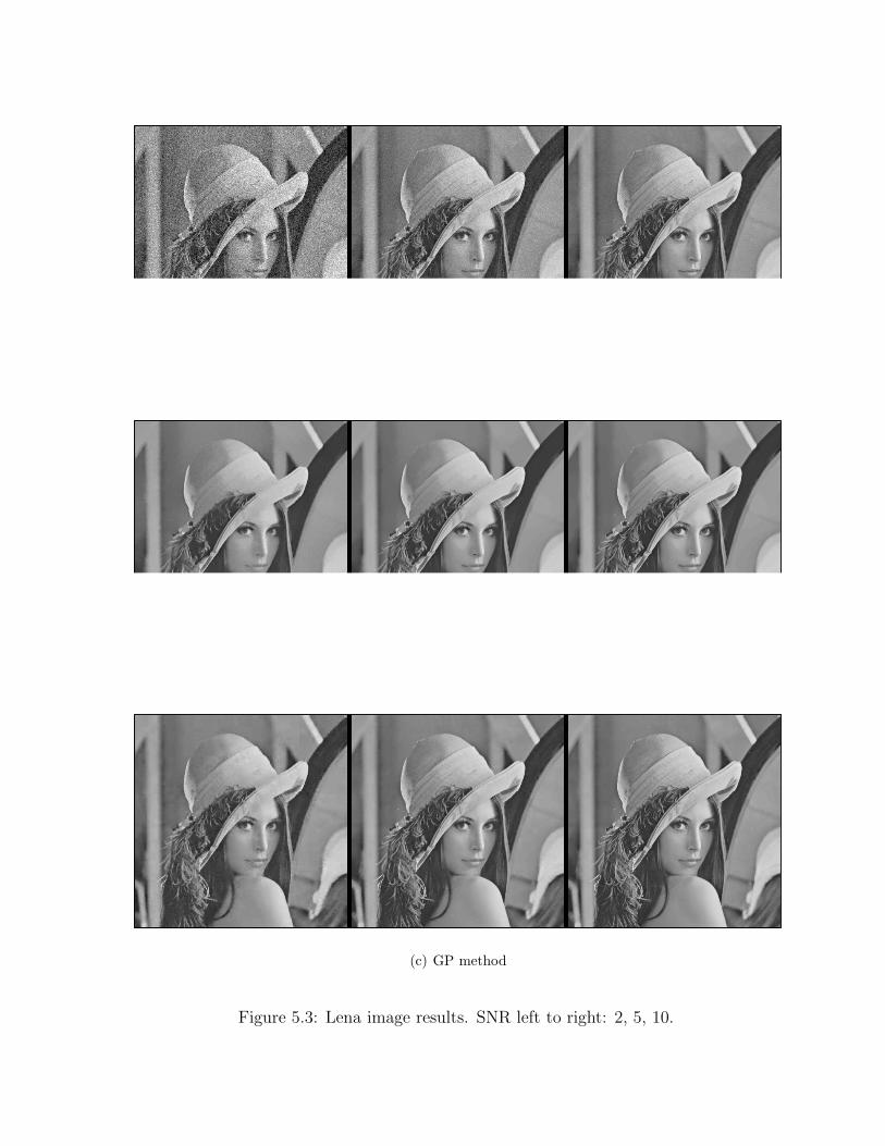
Chapter 5. Image denoising 60
(a) noise added
(b) NL means
(c) GP method
Figure 5.3: Lena image results. SNR left to right: 2, 5, 10.
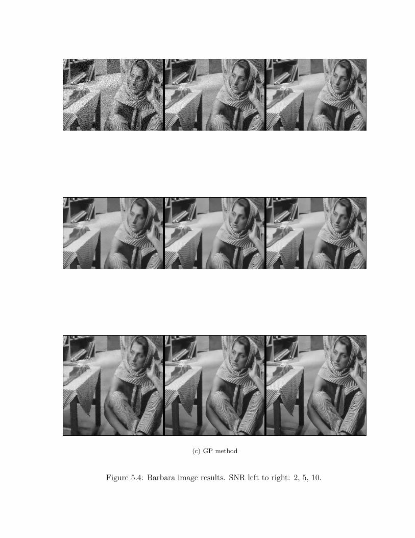
Chapter 5. Image denoising 61
(a) noise added
(b) NL means
(c) GP method
Figure 5.4: Barbara image results. SNR left to right: 2, 5, 10.
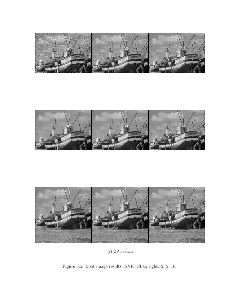
Chapter 5. Image denoising 62
(a) noise added
(b) NL means
(c) GP method
Figure 5.5: Boat image results. SNR left to right: 2, 5, 10.
Chapter 6
Concluding remarks
6.1 Summary of thesis
In this thesis, we have treated microarray spatial artefact/trend removal and image de-
noising as essentially the same problem – the decomposition of data into spatially in-
dependent and dependent components. We showed that both problems can be solved
using very similar methods. We presented a method using Gaussian processes for regres-
sion with a new type of covariance function, which can be used with any grid dataset.
Through experiments in both application domains, we have shown that our method per-
forms favourably compared to well-established methods in the both literatures.
However, we find that our method performs best in the case of medium-to-low en-
ergy in the spatially-independent component relative to the dependent component; this
corresponds to the case of (more realistic) medium-to-low level of noise in image denois-
ing. The performance improvement over other methods is less impressive for microarrays
with low-energy spatial artefacts and images with high noise levels, where the indepen-
dent component plays a more significant role in the data. It may be that the problem is
simply too difficult, and that little can be done beyond small improvements, which are
achievable by simple algorithms. One can justify this intuition by asking probably the
63
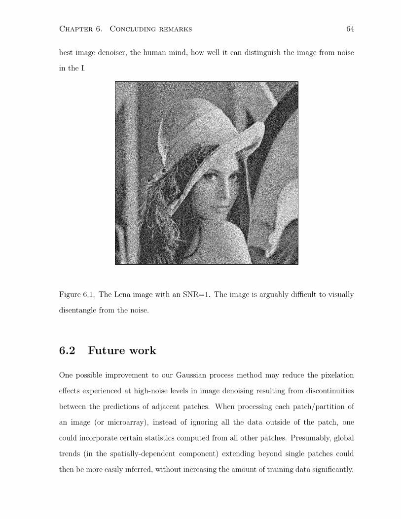
Chapter 6. Concluding remarks 64
best image denoiser, the human mind, how well it can distinguish the image from noise
in the Lena image with an SNR=1 (see Figure 6.1).
Figure 6.1: The Lena image with an SNR=1. The image is arguably difficult to visually
disentangle from the noise.
6.2 Future work
One possible improvement to our Gaussian process method may reduce the pixelation
effects experienced at high-noise levels in image denoising resulting from discontinuities
between the predictions of adjacent patches. When processing each patch/partition of
an image (or microarray), instead of ignoring all the data outside of the patch, one
could incorporate certain statistics computed from all other patches. Presumably, global
trends (in the spatially-dependent component) extending beyond single patches could
then be more easily inferred, without increasing the amount of training data significantly.
Chapter 6. Concluding remarks 65
Pixelation might be reduced as continuity across patches might be more encouraged. One
possibly useful statistic would be the mean of each other patch. The covariance between
means and single grid points needs to be handled slightly differently than between two
grid points.
Speeding up our algorithm for large image/microarray datasets is of considerable
practical importance. There are a number of directions one could take to achieve this.
One is to approximate the inverse of the covariance matrix, whose computation is very
time-consuming when learning the hyperparameters, the dominant step with respect to
time complexity. To this end, one may use a low-rank approximation to the covariance
matrix as in the Nystrom approximation [22], or approximate the Cholesky factorization
as in [6]. A second direction is to use a subset of the data selected by some reasonable
criteria to train the hyperaparameters; we achieved a similar reduction in training data
using our medians scheme when applying our algorithm to microarray data, but more
general methods exist. A review of these methods can be found in Chapter 8 of Rasmussen
and Williams’ book ([14]).
On the theoretical side, further analysis of our use of pseudo-inputs in our covariance
function can be conducted. Our pseudo-inputs in fact are a subset of the noisy-outputs.
Having the covariance between outputs depend on other (noisy) outputs may be viewed
with suspicion. However, the fact that our method performs well in experiments suggests
something has been gained. A new interpretation of what we are doing may lead to a
more principled framework and allay our anxieties.
Finally, a comparision of the image denoising performance with state-of-the-art com-
mercial applications such as Noise Ninja and Neat Image would be interesting.
Bibliography
[1] P. Abrahamsen. A review of gaussian random fields and correlation functions. Tech-
nical Report 917, Norwegian Computing Center, Oslo, Norway, 1997.
[2] A. Buades, B. Coll, and J. M. Morel. A review of image denoising algorithms, with
a new one. Multiscale Modeling & Simulation, 4(2):490–530, 2005.
[3] A. Buades and J. M. Morel. A non-local algorithm for image denoising. In IEEE
Computer Vision and Pattern Recognition or CVPR, pages II: 60–65, 2005.
[4] N. A. C. Cressie. Statistics for Spatial Data. J. Wiley and Sons, New York, 1993.
[5] D. L. Donoho and I. M. Johnstone. Ideal spatial adaptation via wavelet shrinkage.
Biometrika, 81:425–455, 1994.
[6] S. Fine and K. Scheinberg. Efficient SVM training using low-rank kernel represen-
tations. Journal of Machine Learning Research, 2:243–264, 2001.
[7] J. C. Huang, Q. Morris, T. R. Hughes, and B. J. Frey. GenXHC: a probabilistic
generative model for cross-hybridization compensation in high-density genome-wide
microarray data. In ISMB (Supplement of Bioinformatics), pages 222–231, 2005.
[8] D. J. C. MacKay. Hyperparameters: optimize, or integrate out? Neural Computa-
tion, 1994.
[9] Q. D. Morris, O. Shai, B. J. Frey, W. Zhang, and T. R. Hughes. Spatial trend
removal - reducing systematic noise in microarrays. in preparation, 2004.
66
Bibliography 67
[10] R. M. Neal. Probabilistic inference using Markov chain Monte Carlo methods.
Technical Report CRG-TR-93-1, Department of Computer Science, University of
Toronto, September 1993.
[11] R. M. Neal. Bayesian Learning for Neural Networks. Number 118 in Lecture Notes
in Statistics. Springer, New York, USA, 1996.
[12] R. M. Neal. Monte Carlo implementation of Gaussian process models for Bayesian
regression and classification. Technical Report no. 9702. Department of Statistics,
University of Toronto, 1997.
[13] C. J. Paciorek. Nonstationary Gaussian processes for regression and spatial mod-
elling, May 15 2003.
[14] C. E. Rasmussen and C. K. I. Williams. Gaussian Processes for Machine Learning.
MIT Press, 2006.
[15] M. Rosenblatt. Random Processes. Springer, New York, 1962.
[16] M. Schena, editor. DNA Microarrays: a practical approach, volume 205 of Practical
approach series. Oxford University Press, Oxford-New York, 1999.
[17] B. Scholkopf and A. J. Smola. Learning with Kernels: Support Vector Machines,
Regularization, Optimization, and Beyond. MIT Press, Cambridge, MA, USA, 2001.
[18] G. K. Smyth and Y. W. Yang. Statistical issues in cDNA microarray data analysis.
Technical report, July 11 2002.
[19] E. Snelson, C. E. Rasmussen, and Z. Ghahramani. Warped Gaussian processes. In
Sebastian Thrun, Lawrence K. Saul, and Bernhard Scholkopf, editors, NIPS. MIT
Press, 2003.
[20] G. Wahba. Spline Models for Observational Data. SIAM, Philadelphia, 1990.
Bibliography 68
[21] C. K. I. Williams and C. E. Rasmussen. Gaussian processes for regression. In
David S. Touretzky, Michael Mozer, and Michael E. Hasselmo, editors, NIPS, pages
514–520. MIT Press, 1995.
[22] C. K. I. Williams and Matthias Seeger. Using the Nystrom method to speed up kernel
machines. In Todd K. Leen, Thomas G. Dietterich, and Volker Tresp, editors, NIPS,
pages 682–688. MIT Press, 2000.
[23] W. Zhang, Q. D. Morris, R. Chang, O. Shai, M. A. Bakowski, N. Mitsakakis, N. Mo-
hammad, M. D. Robinson, R. Zirngibl, E. Somogyi, N. Laurin, E. Eftekharpour,
E. Sat, J. Grigull, Q. Pan, W. T. Peng, N. Krogan, J. Greenblatt, M. Fehlings,
D. van der Kooy, J. Aubin, B. G. Bruneau, J. Rossant, B. J. Blencowe, B. J. Frey,
and T. R. Hughes. The functional landscape of mouse gene expression. Journal of
Biology, 3(5), 2004.