Using EPECs to Model Bilevel Games in Restructured ... EPECs to Model Bilevel Games in Restructured...

Using EPECs to Model Bilevel Games in Restructured Electricity Markets with

Locational Prices

Xinmin Hu and Daniel Ralph

February 2006

CWPE 0619 and EPRG 0602

These working papers present preliminary research findings, and you are advised to cite with caution unless you first contact the

author regarding possible amendments.

Using EPECs to model bilevel games in restructured electricity

markets with locational prices

Xinmin Hu

Australian Graduate School of Management

University of New South Wales, NSW 2052, Australia

Daniel Ralph

Judge Business School

The University of Cambridge, CB2 1AG, Cambridge, UK

We study a bilevel noncooperative game-theoretic model of restructured electricity markets, with loca-

tional marginal prices. Each player in this game faces a bilevel optimization problem that we remodel

as a mathematical program with equilibrium constraints, MPEC. The corresponding game is an exam-

ple of an EPEC, equilibrium problem with equilibrium constraints. We establish sufficient conditions

for existence of pure strategy Nash equilibria for this class of bilevel games and give some applications.

We show by examples the effect of network transmission limits, i.e. congestion, on existence of equi-

libria. Then we study, for more general EPECs, the weaker pure strategy concepts of local Nash and

Nash stationary equilibria. We pose the latter as solutions of mixed complementarity problems, CPs,

and show their equivalence with the former in some cases. Finally, we present numerical examples of

methods that attempt to find local Nash equilibria or Nash stationary points of randomly generated

electricity market games. The CP solver PATH is found to be rather effective in identifying Nash

stationary points.

Keywords: electricity market, bilevel game, MPEC, EPEC, Nash stationary point, equilibrium con-

straints, complementarity problem

JEL classification: C61, C62, C72, Q40

1

1 Introduction

Game-theoretic models are employed to investigate strategic behavior in restructured or deregulated

electricity markets — see Berry et al. (1999), Cardell et al. (1997), Hobbs et al. (2000), Nasser (1998),

Oren (1997), Seeley et al. (2000), Stoft (1999) to mention just a few references — and, of course, more

general markets. Such models depend on the structure and rules of the market, and, for electricity

and other distributed markets, the way network constraints are handled. Using the bilevel electricity

market game of Berry et al. (1999) as a jumping-off point, this paper seeks more general modeling

paradigms of bilevel games. The thrust of our investigation is twofold. First, in the context of Berry

et al. (1999), we seek to understand when pure strategy Nash equilibria exist and when they may

not. Second, for more general bilevel games, by modeling each player’s problem as a mathematical

program with equilibrium constraints, MPEC, we recast bilevel games as equilibrium problems with

equilibrium constraints, EPECs. Stationarity theory for MPECs allows us to introduce Nash stationary

points, a weakening of the Nash equilibrium concept, for EPECs and show that the standard mixed

complementarity problem (CP) format captures such points. This opens the way to analysis and

algorithms that seem new to bilevel games.

A particular motivation is the area of noncooperative games that model electricity markets over

a network of generators and consumers in the style of Berry et al. (1999), see also Backerman et al.

(2000), Cardell et al. (1997), Hobbs et al. (2000); and also Hu et al. (2004) for a brief review of these

and related market models. A coordinator or central operator, called an independent system operator

(ISO), schedules the dispatch quantities, prices and transmission of electricity. To do so the ISO solves

an optimization problem that relies on the configuration and electrical properties of the network, and on

bids from generators and consumers (e.g. retailers) that propose how price should vary with quantity.

This results in a game that has a bilevel structure; in particular, the ISO’s optimization problem,

which lies on the lower level, gives rise to non-differentiability and non-quasiconcavity of an individual

participant’s profit function on the upper level.

In broader terms, we study games in which each player faces a bilevel maximization problem that can

be modeled as an MPEC. Such problems have nonconvex constraints and therefore may have multiple

local maxima. Thus the corresponding game, an EPEC, may not have any (pure strategy) Nash

equilibria in pathological instances, e.g., Example 12 in §3.3. See also Berry et al. (1999, Footnote

8, p.143) and Weber and Overbye (1999). This motivates development of alternatives to the Nash

equilibrium concept, aimed at model formats that are suitable for application of powerful mathematical

programming solvers. Our computational approach is to seek points such that each player’s strategy

satisfies the stationary conditions for his or her MPEC.

The meaning of the situation when a Nash equilibrium does not exist is, by some leagues, beyond

the scope of this paper. Without a Nash equilibrium, the questions “Is the model deficient”? and “Is

the market unstable?” point to future investigations that might study the gap between models and

2

their application in policy, commerce, and regulation.

While the emphasis of this paper is on methodology, a companion paper Hu et al. (2004) gives a

comprehensive treatment of the economic implications of numerical results for the electricity market

model of Berry et al. (1999), e.g. comparisons of market designs. Both papers are derived from the

first author’s PhD dissertation, Hu (2003). A preliminary version of this paper was presented in Hu

and Ralph (2001).

An alternative complementarity problem approach to EPECs in electricity markets is given in

Xian et al. (2004). The paper Leyffer and Munson (2005) gives various complementarity and MPEC

reformulations of EPECs in multi-leader multi-follower games. See also the PhD dissertation Ehren-

mann (2004a); various applications in economics such as Ehrenmann (2004b), Ehrenmann and Neuhoff

(2003), Hu et al. (2004), Murphy and Smeers (2002), Su (2004a), Yao et al. (2005); and the algorithm

investigation Su (2004b).

The paper is organized as follows. Section 2 briefly reviews the formulation of the ISO’s problem and

the associated bilevel game of Berry et al. (1999). Section 3 is mainly a study of sufficient conditions

for existence of pure strategy Nash equilibria for the game scenario in which only the linear part of the

cost/benefit function is bid, the so-called bid linear-only or bid-a-only scenario. It also gives examples

showing how transmission limits may (not) affect existence of Nash equilibria. In this section the

network and associated pricing and dispatch problem are implicit, which simplifies the format of the

game at the expense of requiring analysis of nonsmooth payoff functions. Section 4 studies more general

bilevel games which are reformulated as EPECs. It proposes local Nash equilibria and Nash stationary

equilibria as weaker alternatives to Nash equilibria, and develops a CP formulation of Nash stationary

points to which standard software can be applied. Finally, in a return to electricity market games, it is

shown that Nash stationary points are actually local Nash equilibria for the bid-a-only game scenario

in some circumstances. Section 5 presents numerical examples of two approaches to finding equilibria.

The first approach is to apply the solver PATH (Dirkse and Ferris, 1995; Ferris and Munson, 1999) to

the CP formulation of Nash stationary conditions, and the second uses a kind of fixed-point iteration,

called diagonalization, that is implemented using the nonlinear programming solver SNOPT (Gill et al.,

2002). PATH is found to be particularly fast and robust regarding finding Nash stationary points —

that turn out to be local Nash equilibria — for a test set of randomly generated EPECs. Section 6

concludes the paper.

2 Bilevel game formulation

2.1 Pricing and dispatch by optimal power flow model

As many others do, we work with a lossless direct current network, which consists of nodes where

generators and consumers are located, and (electricity) lines or links connecting nodes; see Chao and

3

Peck (1997). For simplicity of notation assume there are N nodes with one generator at each node

i = 1, . . . , s and one consumer at each node i = s+1, . . . , N . This ordering of players does not play any

role in the mathematical analysis other than simplifying notation and does not restrict us from multiple

players of the same type at any node. However in this paper we do not model an interesting situation

where one generator may own several generating units at different nodes. For further simplicity, only

two types of network constraints (power balance and line flow constraints) are included in the ISO’s

social cost minimization problem.

The market works as follows. Generators/consumers bid nominal cost/utility functions to the ISO.

To dispatch generation and consumption, the ISO determines the quantities of generation/consumption

for generators/consumers by minimizing the nominal social cost, the difference between the total cost

and the total utility, subject to network constraints. (Equivalently, the ISO could maximize nominal

social welfare.) The prices at each node are set to the nominal marginal cost/utility at a given node,

reflecting the fact that higher prices may be needed to curb demand at network nodes to which

transmission constraints limit delivery of electricity. For further development of the locational or

nodal pricing idea, see Chao and Peck (1997), Hogan (1992).

Various forms of cost/benefit functions are assumed in literature with or without start-up costs for

generators, and in practical markets the functions are step functions. In this paper, we use a quadratic

form without a start-up cost as in Berry et al. (1999), Cardell et al. (1997), Weber and Overbye (1999).

To this end, the cost function of a generator at node i has the form ci(qi) = aiqi + biq2i with qi ≥ 0

and the utility function of a consumer at node j has the form −cj(qj) = −ajqj − bjq2j with qj ≤ 0.

Let Q = Q(b) = diag(b1, · · · , bN ), a = (a1, . . . , aN )T , q = (q1, . . . , qN )T . A link from node i to node j

is denoted ij and its transmission limit is Cij . The vector of transmission limits is Cmax. Then, the

optimal power flow problem faced by the ISO can be written, e.g. Wu and Varaiya (1997), as:

minimizeq

qT Qq + aT q

subject to q1 + · · · + qN = 0

−Cmax ≤ Φq ≤ Cmax

qi ≥ 0, i = 1, . . . , s, qi ≤ 0, i = s + 1, . . . , N

(1)

where Φ is a K × N matrix of distribution factors (Wood and Wollenberg, 1996) or injection shift

factors (Liu and Gross, 2004); and K denotes the number of transmission lines in the network. The

distribution factors give linear approximations of the first order sensitivities of power flows with respect

to changes of net nodal injections. Distribution factors are determined by three sets of parameters: a

reference node (always labelled node 0 in this paper), the topology of the network (connections between

nodes by lines), and the electrical properties of lines such as susceptance. It worth pointing out that

market outcomes are independent of the choice of the reference node.

Observe that the optimal power flow problem is a quadratic program with a nonempty feasible set;

and has a strictly convex objective if each bi > 0.

The next result is well known, e.g. (i) by discussion in Luo et al. (1996, pp.169-171) and (ii) by the

4

more general results surveyed in Bonnans and Shapiro (1998, Section 5):

Lemma 1 Let Cmax be a positive vector.

(i) Fix b > 0, and consider a as a parameter vector in (1). Then problem (1) is solvable for any a,

its optimal solution q∗ = q∗(a) is unique, and q∗(a) is a piecewise linear mapping in a.

(ii) Consider a and b as parameters in (1). For any b > 0 and any a, (1) is solvable, the optimal

solution q∗ = q∗(a, b) is unique, and q∗(a, b) is a locally Lipschitz mapping with respect to (a, b).

2.2 A bilevel game

Now, the question is how profit-seeking generators and consumers behave under such a market mech-

anism. We present a model from Berry et al. (1999), which is also considered in Backerman et al.

(2000), that is designed to address this question.

Let Aiqi + Biq2i be the actual cost incurred by generator i to generate qi ≥ 0 units of electricity.

Similarly, −Ajqj − Bjq2j = Aj(−qj) − Bj(−qj)

2 is the actual utility received by consumer j when

consuming −qj ≥ 0 units of electricity. Given participant i’s bid (ai, bi) and quantity qi, the market

price at node i is the marginal price, i.e. the derivative ai + 2biqi of its bid function at qi. Thus a

generator at node i receives revenue (ai + 2biqi)qi, and its profit maximization problem is:

maximizeai,bi,q

(ai + 2biqi)qi − (Aiqi + Biq2i )

subject to A i ≤ ai ≤ Ai

B i ≤ bi ≤ Bi

q = (q1, . . . , qi, . . . , qN ) solves (1) given (a−i, b−i)

(2)

where a−i = (a1, . . . , ai−1, ai+1, . . . , aN ), b−i = (b1, . . . , bi−1, bi+1, . . . , bN ); and A i (B i) and Ai (Bi)

are the lower bound and upper bound on ai (bi), respectively. For the rest of this paper, we assume

that 0 ≤ Ai ≤ Ai ≤ Ai and 0 < Bi ≤ Bi ≤ Bi.

Formally, (2) is called a bilevel program, where the lower-level program is the parametric prob-

lem (1); thus {(2)}Ni=1 is a bilevel game. In addition, since the lower-level problem is convex, we can

represent it equivalently via its stationary conditions, which form an “equilibrium” system, as explained

in §4.2. This converts the game to an EPEC; see Outrata (2003) for general formulation of EPECs.

3 Nash equilibria in the electricity market model

As suggested in Berry et al. (1999), and shown explicitly in Example 12 to follow, existence of pure

strategy Nash equilibria is not guaranteed for the electricity market game {(2)}Ni=1. However, given

Lemma 1, the existence of mixed strategy Nash equilibria for {(2)}Ni=1 is a straightforward consequence

of a classical result Balder (1995, Proposition 2.1) for games with finitely many players, each of whom

has a continuous payoff function and compact set of pure strategies.

5

Our main interest is the existence of (pure strategy) Nash equilibria of the game {(2)}Ni=1: see Berry

et al. (1999), Younes and Ilic (1999), Hobbs et al. (2000), where generators and consumers bid only

ai while leaving bi = Bi > 0 fixed, or, equivalently, each player’s bid has the form (ai, Bi). This is

referred to as the bid-a-only or bid linear-only scenario. The focus on bid-a-only games is for two main

reasons. First, the bid-a-b game, in which each player bids (ai, bi), has multiple equilbria in general,

which makes its use in economic comparisons fraught because it is not apparent which equilibrium to

select, whereas the bid-a-only game and its bid-b-only counterpart both tend to have unique equilibria

when these exist; see Hu (2003, Chapter 5). Second, the theoretical analysis of the bid-a-only game,

to follow, is a reasonable surrogate for that of the bid-b-only game which is analysed in detail in Hu

(2003, Chapter 5, 6). Nevertheless we do attempt to solve all three types of games in Section 5 because

the modeling and computational framework makes it convenient to do so, and the bid-a-b games have

a different numerical flavor from the others.

While computational methods or policy issues are the topics in papers cited above, we look at basic

properties of the market model that relate to existence of Nash equilibria. We set up our notation in

§3.1 and give sufficient conditions for existence of Nash equilibria in §3.2. In §3.3 we give examples of

existence of Nash equilibria, or lack thereof.

3.1 Notation for the bid linear-only game scenario

For i = 1, . . . , N , bi = Bi is fixed. That is, we assume Bi is known to the ISO and all players and,

as a result, the quadratic coefficients are not strategic variables. The multi-strategy vector a may be

written (ai, a−i) when considering player i. For example, the optimal dispatch referred to in Lemma 1

will be denoted by q∗(a) or q∗(ai, a−i) in the context of player i, whose profit function is

fi(ai, a−i) = (ai − Ai)q∗i (ai, a−i) + Biq

∗i (ai, a−i)

2. (3)

This mapping is piecewise smooth on A by Lemma 1, where

Ai = [A i, Ai], A =

N∏

i=1

Ai.

The ith player’s profit or utility maximization problem is

maximizeai

fi(ai, a−i) subject to ai ∈ Ai. (4)

In this paper we focus on games of complete information, that is, each player knows not only its

own payoff functions, but other players’ payoff functions including their strategy spaces as well. It is

worth noting that the above game {(4)}Ni=1 has a classical format in that each player’s strategy set is

convex and compact. In particular, the network and the associated pricing and dispatch problem are

implicit rather than explicit, which allows a simple format of the game although the payoff functions

are not smooth but piecewise smooth. We also note, for reference in the next subsection, that whatever

6

bids a−i are made by other players, Player i’s strategy can always be chosen to make his or her profit

nonnegative: Ai ∈ Ai from our assumptions in subsection 2.2, and (3) gives fi(Ai, a−i) ≥ 0.

3.2 Existence of Nash equilibria

An often-cited sufficient condition for the existence of (pure strategy) Nash equilibria is quasi-concavity

of players’ profit functions on their whole strategy spaces. However, Theorem 2 below assumes, for

each player, nonemptiness and convexity of the subset of its strategies with nonnegative profit, and

quasi-concavity of that player’s profit function over this subset. We omit the proof which is almost

identical to that of the standard existence theorem; see, for example Myerson (1991, pp. 138-140).

Theorem 2 Given a game with (a finite number) N of players for which the ith player has the payoff

function fi(xi, x−i) and the strategy set Xi, assume the following conditions hold:

(i) the strategy space Xi ⊆ Rni is a nonempty compact set;

(ii) for each x−i in X−i =∏

j:j 6=i Xj , the set Xi(x−i) := {xi ∈ Xi : fi(xi, x−i) ≥ 0} is nonempty

and convex;

(iii) for each x−i ∈ X−i, the function fi(·, x−i) is quasi-concave on Xi(x−i); and

(iv) fi(·) is continuous in∏N

i=1 Xi.

Then the game has at least one Nash equilibrium such that every participant’s profit is nonnegative.

We begin the analysis of the game {(4)}Ni=1 with some notation. Consider the mapping ai 7→

q∗i (ai, a−i) which we denote q∗i (·, a−i). Given a−i, let ∂iq∗i (ai, a−i) denote the generalized gradient of

Clarke (1993) of this mapping. (As an aside, we give the definition of generalized gradient ∂f(x0)

of an arbitrary locally Lipschitz function f : Rn → R at x0 ∈ Rn, using the classical result that the

function is differentiable almost everywhere; see Clarke (1993) for details. The generalized gradient can

be defined as the convex hull of limit points of sequences {∇f(xk)} over all sequences {xk} converging

to x0 such that ∇f(xk) exists for each k. The local Lipschitz property ensures that the generalized

gradient is nonempty and compact.) Our first result is technical. Its proof can be given from first

principles; see the online Appendix.

Proposition 3 For any participant i = 1, . . . , N , its dispatch function q∗i (·, a−i) is a non-increasing

function of its own bid ai given others’ bid vector a−i. Moreover, the directional derivative of q∗i (·, a−i)

along any direction u ∈ R satisfies

|q∗i′(ai, a−i;u)| ≤ |u|/(2Bi).

As a result, ∂iq∗i (ai, a−i) ⊆ [−1/(2Bi), 0].

7

ia

*iq

Dispatch for a generator

Dispatch for a consumer

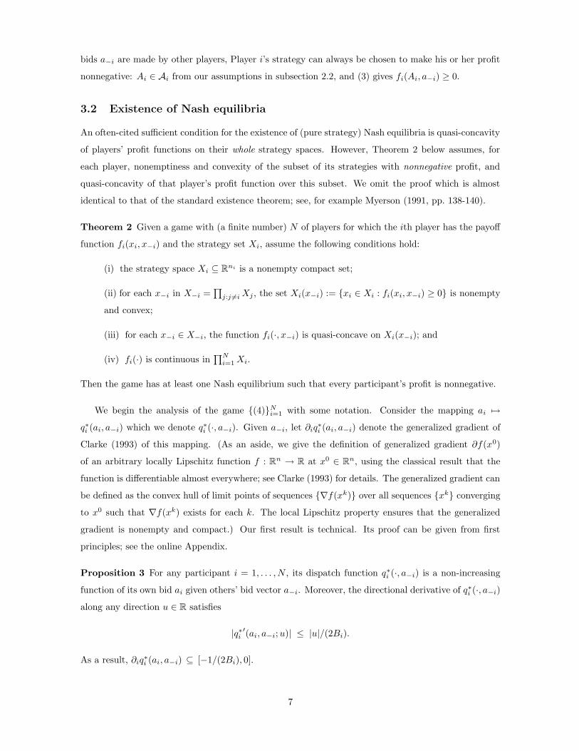
Figure 1: Sketch of piecewise linear dispatch for generators and consumers

By Lemma 1, there is a number W (depending on the number of pieces of the KKT system of

(1)) such that, given a−i, the derivative q∗i′(ai, a−i) of q∗i (·, a−i) exists except at the breakpoints

0 < w1 = w1(a−i) ≤ w2 = w2(a−i) ≤ · · · ≤ wW = wW (a−i). Note that some of the points wj may

coincide for certain a−i for which there are fewer than W breakpoints. We sketch the dispatch as

a piecewise linear function of its bid in Figure 1 and we will fix these notations for the rest of this

subsection. As an application of Proposition 3, Lemma 1, and Theorem 2, we have the following

theorem, whose proof is given in the online Appendix.

Theorem 4 Suppose player i’s dispatch q∗i (·, a−i) satisfies the following conditions for each a−i and

breakpoint wj with fi(wj , a−i) > 0:

if i is a generator: limv↑wj

q∗i′(v, a−i) ≥ lim

v↓wj

q∗i′(v, a−i), (5)

if i is a consumer: limv↑wj

q∗i′(v, a−i) ≤ lim

v↓wj

q∗i′(v, a−i), (6)

where v ↑ wj means v → wj , v < wj ; and v ↓ wj is similarly defined. Then the game {(4)}Ni=1 has at

least one Nash equilibrium such that each generator’s profit and consumer’s utility is nonnegative.

The next three results are applications of Theorem 4. In each case, the conditions (5) and (6) can

be established, yielding existence of a Nash equilibrium. Such a Nash equilibrium may not be unique

but we can nevertheless show that, at a given Nash equilibrium, each generator with positive profit

has a unique optimal response to the other player’s equilibrium strategies.

First, we apply Theorem 4 to uncongested networks where all players participate in the market.

Proposition 5 If, for any a ∈ A, the ISO’s dispatch yields uncongested flows and is nonzero for each

player, then there exists a Nash equilibrium for {(4)}Ni=1. Moreover, given other players’ strategies at

such a Nash equilibrium, the optimal strategy of each player is unique.

Proof Since for any bid a, every generator or consumer has nonzero dispatch, the KKT conditions

of the ISO’s problem (1) contains the following linear system:

a1 + 2B1q1 + λ = 0, · · · , aN + 2BNqN + λ = 0, q1 + · · · + qN = 0

8

where λ is the Lagrange multiplier corresponding to the constraint q1 + · · · + qN = 0. As a result,

q∗i (ai, a−i) is a linear function for (ai, a−i) ∈ A, so (5) and (6) hold trivially. Therefore, by Theorem 4,

there is at least one Nash equilibrium. Uniqueness of each player’s best response to the others’ strategies

follows if we have strict concavity of profit functions. In fact, q∗i is strictly decreasing in ai (see (8) for

its formula), therefore, by Proposition 3, we have −1/(2Bi) ≤ q∗i′ < 0. Strict concavity now results

from (3). �

Second, we consider the case where consumers are symmetric (identical) and are price takers (i.e.

do not bid, rather their utility functions are known by all players and the ISO), but generators may

have different generation costs. This is a weakening of a more typical assumption that generation costs

are symmetric, e.g. Green and Newbery (1992), Klemperer and Meyer (1989). Here some generators

may be out of the market, unlike Proposition 5. Using symmetric consumer utilities ensures that all

consumers have nonzero consumption, or all have zero consumption, which makes the mathematical

analysis tractable.

Proposition 6 Consider a network with capacities of all lines large enough so that there is no potential

congestion. Assume that consumers have the same benefit function (i.e., they have the same Ai, Bi)

which is known to the ISO and all players. Then there exists at least one Nash equilibrium for the

game {(4)}Ni=1. Moreover, with respect to any such Nash equilibrium, the optimal strategy of each

generator with a positive profit is unique.

Proof It suffices to establish (5) for a given generator i by fixing a−i and a breakpoint w = wj of

q∗i (·, a−i) such that q∗i (w, a−i) > 0, and considering the derivative q∗i′(v, a−i) for v near w but v 6= w.

In general, the vector (q, λ, µ) of optimal dispatches and the corresponding Lagrange multipliers

satisfies the following KKT conditions of (1) without line capacity constraints:

a1 + 2B1q1 + λ + µ1 = 0 · · · , aN + 2BNqN + λ + µN = 0, q1 + · · · + qN = 0,

qkµk = 0, qk ≥ 0, µk ≤ 0, k: generator,

qkµk = 0, qk ≤ 0, µk ≥ 0, k: consumer.

The KKT system can be used to derive the market price, which is uniform across the market, as

−λ(ai, a−i) =(

∑

k∈K

ak

2Bk

)/(

∑

k∈K

1

2Bk

)

,

where K = K(ai, a−i) = {k : q∗k(ai, a−i) 6= 0}, since µk = 0 for k ∈ K. The KKT system then gives

−λ(ai, a−i) = ak + 2Bkq∗k(ai, a−i) for any k ∈ K. (7)

It follows that q∗i (·, a−i) is differentiable at ai if i ∈ K and K(v, a−i) = K for v near ai, with

q∗i′(ai, a−i) = −

(

1 + Li

)

/(2Bi) where − 1/Li =∑

k∈K

Bi/Bk. (8)

9

We need to establish some monotonicity properties. Suppose the generator i has i ∈ K = K(ai, a−i).

From (7) with k = i, the generalized gradient of the market price with respect to ai is the set

1 + 2Bi∂iq∗i (ai, a−i), which contains only nonnegative values by Proposition 3. That is, price is non-

decreasing in ai. Next consider a generator k 6∈ K, i.e. q∗k(ai, a−i) = 0. We claim for v < ai that

q∗k(v, a−i) = 0. For if q∗k(v, a−i) > 0 then (7) at ai = v and the monotonicity of price imply q∗k(v, a−i)

is nondecreasing as v ↑ ai; this can only happen, given continuity of q∗k(·, a−i) at ai, if q∗k(v, a−i) = 0.

Now let w be a breakpoint as above. Then q∗i (·, a−i) is differentiable at v near w with v 6= w.

Suppose that generator i unilaterally raises its linear bid by a small amount from w to v > w. By

continuity of the vector q∗(·, a−i), each quantity q∗k(v, a−i) stays positive for k ∈ K(w, a−i), hence

K(v, a−i) ⊇ K(w, a−i) for v > w, v near w.

Suppose instead that player i unilaterally lowers its linear bid by a small amount to v < w. As before,

we see that K(v, a−i) contains K(w, a−i), but we also claim the converse, namely

K(v, a−i) = K(w, a−i) for v < w, v near w.

To see this, first note, since consumers are symmetric and total production is positive for v near w, that

each consumer k belongs to K(v, a−i). Second, for a generator k with q∗k(w, a−i) = 0 we have already

seen that q∗k(v, a−i) = 0 when v < w. The claimed equality follows. In light of these relationships and

(8), with ai = v near but not equal to w and K = K(v, a−i), the inequality (5) can be easily verified.

The uniqueness claim follows from the fact that all these participants’ profit functions are strictly

concave when their strategies are restricted to those with strictly positive dispatch. �

Finally, we apply Theorem 4 to a two-node network with multiple generators and consumers at each

node and a transmission capacity limit C on the only line between the two nodes. The line may be

congested for some dispatches. This result has relevance, for example, in the New Zealand electricity

market, which is a nodal pricing market where the South Island has 41% of the market generation

capacity and 36% of market demand, while the North Island has the remainder of generation capacity

and demand, and the two islands are connected by a single high voltage direct current link. See David

Butchers & Associates (2001) for more details for the New Zealand market.

Proposition 7 Consider a network with two nodes and one line linking the two nodes with a trans-

mission capacity limit C > 0 on the line. At each node, there may be multiple generators and/or

consumers. If all consumers have the same benefit function, which is known to the ISO and all gen-

erators, and they do not bid strategically, then there exists at least one Nash equilibrium for the

game {(4)}Ni=1. Moreover, with respect to any such Nash equilibrium, the optimal strategy of each

generator with a positive profit is unique.

Proof The proof is almost the same as that of Proposition 6. For example, let i be a generator,

a−i be fixed, and S = S(ai, a−i) denote the set of generators k such that q∗k(ai, a−i) > 0. The KKT

10

conditions for this problem yield

−λ(ai, a−i) =(

∑

k∈S

ak

2Bk

+ C)/(

∑

k∈S

1

2Bk

)

,

and −λ(ai, a−i) = ai + 2Biq∗i (ai, a−i) if i ∈ S. The proof can be completed as an exercise. �

3.3 Effects of transmission constraints on the set of Nash equilibria

In this section, we present two simple networks (see Figure 2) to see the effect of congestion on the

existence of Nash equilibria of the bid-a-only game {(4)}Ni=1. In the two-node case, the transmission

limit leads to a continuum of Nash equilibria, while the transmission limit in a three-node network

may result in non-existence of any Nash equilibrium.

The calculation of Nash equilibria for these two networks follows the classical idea of finding the

intersection of every individual’s best response curves. The best response function of participant i is

a possibly set-valued mapping which maps a−i to the set argmax ai{fi(ai, a−i) : ai ∈ Ai}. In the

following examples, A i = 0, Ai = 100.

0,)( 121111 ≥+= qqqqc 0,10)( 2

22222 ≤+= qqqqc

Node 1 Node 2

(a)

Node 0

Node 1Node 2

0,1.02)( 020000 ≥+= qqqqc

0,1.0)( 121111 ≥+= qqqqc0,05.04)( 2

22222 ≤+= qqqqc

(b)

transmission capacity limit

Figure 2: Two networks, location of generators and consumers and their cost/utility functions. Arrows

show extraction or injection of electricity.

Example 8 (two-node network, uncongested) Consider a two-node network with one generator

and one consumer and their true cost/benefit functions shown in Figure 2(a).

When there is no capacity limit on the line, Proposition 5 tells that there exists a Nash equilibrium

and the equilibrium point is (a∗1, a

∗2) = (3.25, 7.75).

Example 9 (two-node network, congested) Now we consider the previous example with a ca-

pacity limit C12 = 1 on the line. Given a bid (a1, a2), the dispatches (a solution to problem (1))

are

q∗1 = −q∗2 =a2 − a1

4when 0 ≤ a2 − a1 ≤ 4, or q∗1 = −q∗2 = 1, when a2 − a1 ≥ 4

or q∗1 = −q∗2 = 0 otherwise.

11

In fact, it can be shown that the best response mappings for the generator and the consumer are

a∗1(a2) =

[a2, 100] if 0 ≤ a2 ≤ 1,

0.3333a2 + 0.6667, if 1 ≤ a2 ≤ 7,

a2 − 4, if a2 ≥ 7,

and

a∗2(a1) =

a1 + 4, if 0 ≤ a1 ≤ 4,

0.3333a1 + 6.6667, if 4 ≤ a1 ≤ 10,

[0, a1], if a1 ≥ 10,

respectively. The intersection of the two best response mappings gives the set of Nash equilibria for

the game, which is {(a1, a2) ∈ R2 : a2 − a1 = 4 and 7 ≤ a2 ≤ 8}.

Generally speaking, congested lines may lead to multiplicity of local Nash equilibria. The mul-

tiplicity may cause ambiguity of economic conclusions based on the equilibria. See debates on this

between Stoft (1999) and Oren (1997) for a Cournot-Nash model representing an electricity market

with two-node and three-node networks.

In general, we have the following corollary, which is different from Proposition 7 in that the consumer

in Corollary 10 participates in strategic bidding and multiple generators are allowed in Proposition 7.

Corollary 10 Consider any two-node, one-line network with only one generator and one consumer

located at different nodes. There always exists at least one Nash equilibrium for {(4)}2i=1 regardless of

capacity limit on the line.

Proof If there is no capacity limit on the line, the corollary is true by Proposition 5. Now assume

that there is a capacity limit C on the line. Consider condition (6) for the consumer (a similar proof

holds for the generator). Fix the generator’s bid a1 ≥ 0, if the capacity limit on the line is just reached

by a dispatch given bid (a1, w), i.e. q∗1 = −q∗2 = C when a2 ≥ w and q∗1 = −q∗2 < C when a2 < w,

where w is a bid by the consumer. So q∗2′ = 0 for a2 > w since q∗2(a1, a2) = −C for a2 ≥ w. Similarly

q∗2′ ≤ 0 for a2 < w (see also Proposition 3). Therefore (6) holds for the consumer. Hence the corollary

follows from Theorem 4. �

Example 11 (three-node network, uncongested) Consider a three-node network given in Fig-

ure 2(b). There are two competing generators and one consumer who does not compete but rather

provides a passive demand function by revealing her true benefit function to the ISO and the two

generators. The true cost and benefit functions are shown in Figure 2(b). Node 2 is chosen as the

reference node and therefore its distribution factors to all three lines are zero. The distribution factors

of node 0 to lines 01, 02, 12 are −0.25,−0.75,−0.25 respectively, and those of node 1 to above lines are

0.25,−0.25,−0.75.

Without any transmission limits on the three lines, we know by Proposition 6 that {(4)}2i=1 has a

Nash equilibrium, which is (a∗1, a

∗2) = (2.2321, 1.4821) shown in Figure 3.

12

Example 12 (three-node network, congested) Next, assume that there is a capacity limit C01 =

0.9 on the line between node 0 and node 1.

The dispatches (only two possible cases in the KKT system of problem (1) are presented here) are

q∗0 = 10 − 3.75a0 + 1.25a1, q∗1 = 10 + 1.25a0 − 3.75a1, q

∗2 = −20 + 2.5a0 + 2.5a1

when a0 − a1 ≤ 0.72 (uncongested situation) or

q∗0 = 8.2 − 1.25a0 − 1.25a1, q∗1 = 11.8 − 1.25a0 − 1.25a1, q

∗2 = −20 + 2.5a0 + 2.5a1

when a0 − a1 ≥ 0.72 (congested situation).

It is easy to see that condition (5) in Theorem 4 is not true for generator 0:

q∗0′(v, a1) |v<a1+0.72 = −3.75 � −1.25 = q∗0

′(v, a1) |v>a1+0.72 .

Therefore, Theorem 4 cannot apply to the game in this example.

for generator 1

1 2 3 4

1

2

3

4 a

a 0

1

(2.3636, 3.4545)

(2.5, 3.5)

(2.1333, 0)

(0, 1.3333)

(3.25, 1.75)

(3.1818, 1.545)

(2.2321, 1.4821)

Nash point

for generator 0

Figure 3: Best response curves without

transmission limit

��

��

��

��

��

(3.64, 2.92)

1 2 3 4 5

1

2

3

4

5

for generator 1 for generator 0

(1.274, 2.837)

(1.274, 1.41883)(2.2, 1.48)

(2.92, 3.64)

(2.337, 3.057)

(2.25983, 1.8975)

(3.141, 1.8975)

(3.9543, 0)

a

a

1

0

(0, 3.383)

Figure 4: Best response curves with one

transmission limit

In fact, the best response functions for the two generators are

a∗0(a1) =

3.9543 − 0.4286a1, if 0 ≤ a1 ≤ 1.8975,

0.0667a1 + 2.1333, if 1.8975 ≤ a1 ≤ 3.057,

a1 − 0.72, if 3.057 ≤ a1 ≤ 3.64,

2.92, if a1 ≥ 3.64,

and

a∗1(a0) =

3.383 − 0.4286a0, if 0 ≤ a0 ≤ 1.274,

0.0667a0 + 1.3333, if 1.274 ≤ a0 ≤ 2.2,

a0 − 0.72, if 2.2 ≤ a0 ≤ 3.64,

2.92, if a0 ≥ 3.64.

It can be clearly seen that there is no Nash equilibrium for the game in this example from Figure 4,

because there is no intersection point for their best response curves.

13

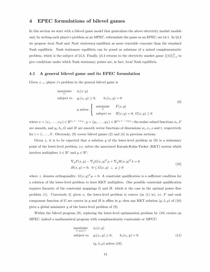
4 EPEC formulations of bilevel games

In this section we start with a bilevel game model that generalizes the above electricity market models

and, by writing each player’s problem as an MPEC, reformulate the game as an EPEC; see §4.1. In §4.2

we propose local Nash and Nash stationary equilibria as more tractable concepts than the standard

Nash equilibria. Nash stationary equilibria can be posed as solutions of a mixed complementarity

problem, which is the subject of §4.3. Finally, §4.4 returns to the electricity market game {(4)}Ni=1 to

give conditions under which Nash stationary points are, in fact, local Nash equilibria.

4.1 A general bilevel game and its EPEC formulation

Given x−i, player i’s problem in the general bilevel game is

maximizexi

φi(x, y)

subject to gi(xi, y) ≥ 0, hi(xi, y) = 0

y solves

minimizey

F (x, y)

subject to H(x, y) = 0, G(x, y) ≥ 0

(9)

where x = (x1, . . . , xN ) ∈ Rn1+···+nN , y = (y1, . . . , yN ) ∈ Rm1+···+mN ; the scalar-valued functions φi, F

are smooth, and gi, hi, G and H are smooth vector functions of dimensions wi, vi, s and t, respectively

for i = 1, . . . , N . Obviously, (9) covers bilevel games (2) and (4) in previous sections.

Given x, it is to be expected that a solution y of the lower-level problem in (9) is a stationary

point of the lower-level problem, i.e. solves the associated Karush-Kuhn-Tucker (KKT) system which

involves multipliers λ ∈ Rs and µ ∈ Rt:

∇yF (x, y) −∇yG(x, y)T µ + ∇yH(x, y)T λ = 0

H(x, y) = 0, 0 ≤ G(x, y) ⊥ µ ≥ 0(10)

where ⊥ denotes orthogonality: G(x, y)T µ = 0. A constraint qualification is a sufficient condition for

a solution of the lower-level problem to have KKT multipliers. One possible constraint qualification

requires linearity of the constraint mappings G and H, which is the case in the optimal power flow

problem (1). Conversely if, given x, the lower-level problem is convex (as (1) is), i.e. F and each

component function of G are convex in y and H is affine in y, then any KKT solution (y, λ, µ) of (10)

gives a global minimizer y of the lower-level problem of (9).

Within the bilevel program (9), replacing the lower-level optimization problem by (10) creates an

MPEC, indeed a mathematical program with complementarity constraints or MPCC:

maximizexi,y,µ,λ

φi(x, y)


(y, λ, µ) solves (10).

(11)

14

The corresponding EPEC is the game {(11)}Ni=1; it well might be called an equilibrium program with

complementarity constraints or EPCC.

When comparing the bilevel program (9) to the MPEC (11) it is helpful to suppose, for each x, that

the lower-level KKT system (10) has a unique solution (y(x), λ(x), µ(x)). This makes it obvious that

there is an equivalence between the associated bilevel game and EPEC, cf. Proposition 16 in the next

subsection. Uniqueness of y(x) follows if the lower-level optimization problem is a convex problem with

a nonempty feasible set (in y given x) and a strictly convex objective function F (·, x). Uniqueness of the

multipliers corresponding to y(x) follows if the standard linear independence constraint qualification,

LICQ, holds for the lower-level optimization problem. The LICQ requires that the active constraints

of H(x, y) = 0, G(x, y) ≥ 0 have linearly independent gradients with respect to y at y(x).

Even with uniqueness of y(x), a difficulty previously discussed is that this mapping is generally

nonsmooth, cf. Lemma 1, and may induce nonconcavity in the composite objective function xi 7→

φi(x, y(x)), hence lead to lack of Nash equilibria. Our computational strategy, rather than attempting

to demonstrate or disprove existence of a Nash equilibrium, will be to apply robust mathematical

programming software as a heuristic for finding points that are likely to be Nash equilibria. That is,

we will search for joint strategies x such that, for each i, xi is stationary for MPEC (11) and, if so,

then check whether xi is a local solution of the MPEC.

4.2 Local Nash equilibria and Nash stationary equilibria

A local solution of (11), given x−i = x∗−i, is a point (x∗

i , y∗, λ∗, µ∗) such that for some neighborhood

Ni of this point, (x∗i , y

∗, λ∗, µ∗) is optimal for (11) with the extra constraint (xi, y, λ, µ) ∈ Ni.

Definition 13 A strategy vector (x∗, y∗, λ∗, µ∗) is called a local Nash equilibrium for the EPEC

{(11)}Ni=1 if, for each i, (x∗

i , y∗, λ∗, µ∗) is locally optimal for the MPEC (11) when x−i = x∗

−i.

We may refer to a global Nash equilibrium, meaning a Nash equilibrium, to distinguish it from a local

Nash equilibrium. While local Nash equilibria seem deficient relative to their global counterparts, we

argue that they have some meaning. Local optimality may be sufficient for the satisfaction of players

given that global optima of nonconcave maximization problems are difficult to identify. Putting it

differently, limits to rationality or knowledge of players may lead to meaningful local Nash equilibria.

For instance, generators may only optimize their bids locally (via small adjustments) due to opera-

tional constraints or general conservativeness. Another limit to rationality is implicit in the simple

nature of the model {(11)}Ni=1 explored in Section 3, e.g., a DC model of an electricity network is an

approximation derived by linearizing a nonlinear AC power flow model in a steady state. Since very

different bids may be better studied using different DC approximations, it is not clear how much more

attractive a global Nash equilibrium would be relative to a local Nash equilibrium of this model.

A further challenge, from the computational point of view, is how to find a local optimizer for

a single player. We adopt the classical strategy from nonlinear optimization in which a system of

15

stationary conditions, that is necessarily satisfied at a locally optimal point, provides the main criterion

for recognizing local optimality. That is, our computational approach to EPECs will be to search for

points that satisfy stationary conditions for each player, and then to verify local optimality if possible.

Therefore we further relax the equilibrium solution concept to allow for a strategy vector (x∗, y∗, λ∗, µ∗)

such that each (x∗i , y

∗, λ∗, µ∗) is stationary, in a sense we define next, for player i’s MPEC.

Given x−i, the MPEC (11) is equivalent to a nonlinear program, NLP,

maximizexi,y,λ,µ

φi(x, y)

subject to gi(xi, y) ≥ 0 : ξgi ≥ 0

hi(xi, y) = 0 : ξhi

∇yF (x, y) −∇yG(x, y)T µ + ∇yH(x, y)T λ = 0 : ηi

H(x, y) = 0 : ξHi

G(x, y) ≥ 0 : ξGi ≥ 0

µ ≥ 0 : wi ≥ 0

G(x, y) ∗ µ = 0 : ζi

(12)

where ∗ denotes the Hadamard or componentwise product of vectors, i.e. G(x, y)∗µ = (G1(x, y)µ1, . . .,

Gs(x, y)µs). The vectors at right, ξgi etc., are multipliers that will be used later.

Thanks to recent developments on MPECs, we will see that the following stationary condition,

which is developed further in §4.3, is sensible for the EPEC {(11)}Ni=1. In the definition we use the

term “point” when we could equally use “strategy” or “equilibrium”.

Definition 14 A strategy (x∗, y∗, λ∗, µ∗) is called a Nash stationary point of the EPEC {(11)}Ni=1 if,

for each i = 1, . . . , N , the point (x∗i , y

∗, λ∗, µ∗) is stationary for (12) with x−i = x∗−i.

The definition of Nash stationary points is justified by Proposition 16, to follow, under the following

constraint qualification. First recall, given a feasible point of a system of equality and inequality

constraints, that an active constraint is a scalar-valued constraint that is satisfied as an equality.

Definition 15 Let (x, y, λ, µ) be feasible for the EPEC {(11)}Ni=1.

(i) Given a player index i, the MPEC active constraints at (xi, y, λ, µ) are the active constraints

of (11) ignoring the orthogonality condition denoted ⊥ (equivalently, the active constraints of

(12) excluding the last block-equation G(x, y) ∗ µ = 0).

(ii) MPEC linear independence constraint qualification, MPEC-LICQ, holds for (11) at (xi, y, λ, µ)

if the gradients, with respect to these variables, of the MPEC active constraints at the point

(x, y, λ, µ) are linearly independent.

(iii) We say that the MPEC-LICQ holds for {(11)}Ni=1 at (x, y, λ, µ) if, for each player i, the MPEC-

LICQ holds for (11) at (xi, y, λ, µ).

16

Proposition 16 Let (x∗, y∗, λ∗, µ∗) be feasible for the EPEC {(11)}Ni=1 and consider the following

statements:

(i) (x∗, y∗) is a local Nash equilibrium of the bilevel game {(9)}Ni=1.

(ii) (x∗, y∗, λ∗, µ∗) is a local Nash equilibrium of the EPEC {(11)}Ni=1.

(iii) (x∗, y∗, λ∗, µ∗) is a Nash stationary point of the EPEC {(11)}Ni=1.

Statement (i) implies statement (ii). Statement (ii) implies statement (iii) if the MPEC-LICQ holds

for the EPEC at (x∗, y∗, λ∗, µ∗).

The proof of this proposition is available in the online appendix of this paper.

Remark 17

(i) NLPs that are formulated from MPECs, as above, are unusually difficult in that they do not

satisfy constraint qualifications that are standard in NLP theory. This difficulty is alleviated by

the MPEC-LICQ. Without the MPEC-LICQ, however, it is possible to have a local minimum

of (12) that is not stationary, hence a local or global Nash equilibrium of the associated EPEC

{(11)}Ni=1 that is not Nash stationary.

(ii) According to Scholtes and Stohr (2001), the MPEC-LICQ holds generically for MPECs, that is,

at all feasible points of “most” problems. This result combined with the above proposition does

not promise, but does give us reasonable hope of finding Nash points, if they exist, by identifying

Nash stationary points.

(iii) Stationarity of (x∗i , y

∗, λ∗, µ∗) for (12), where x−i = x∗−i, is equivalent by Anitescu (2000) to

a kind of MPEC stationarity called strong stationarity. See Fletcher et al. (2002), Scheel and

Scholtes (2000) for related discussions of stationarity conditions in MPECs.

4.3 Mixed complementarity problem formulation

We turn to a (mixed) CP formulation of the Nash stationary point conditions of an EPEC. This formu-

lation is an aggregation of the KKT systems of (12) for each player. We call this the complementarity

problem (CP) formulation of the EPEC {(11)}Ni=1; it is referred to in Hu (2003), Hu et al. (2004) as

the All-KKT system.

The Lagrangian function for player i’s MPEC (12) is, omitting the arguments (x, y) from the

functions on the right:

Li(x, y, λ, µ, ξgi , ξh

i , ηi, ξGi , ξH

i , ζi)

= φi + gTi ξg

i + hTi ξh

i + (∇yF −∇yGT µ + ∇yHT λ)T ηi

+µT wi + HT ξHi + GT ξG

i + (G ∗ µ)T ζi.

17

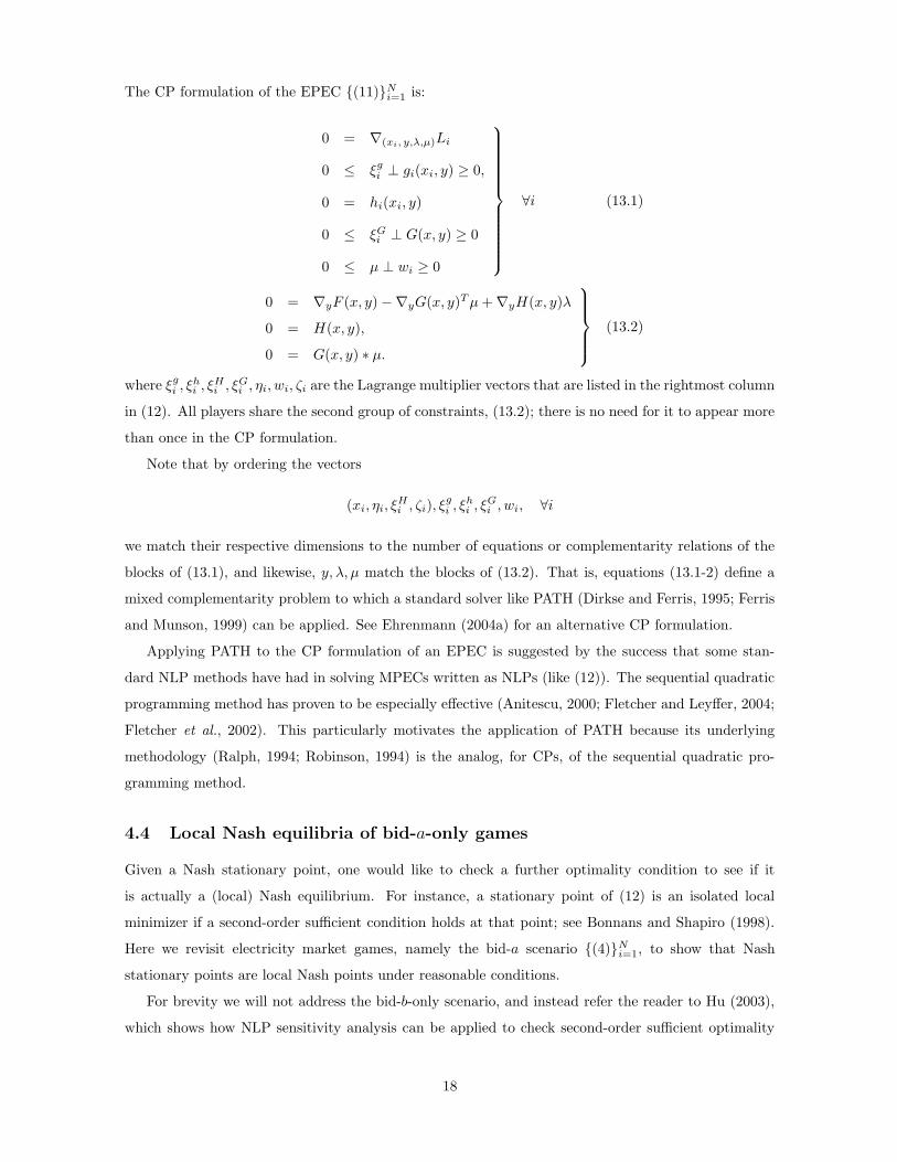
The CP formulation of the EPEC {(11)}Ni=1 is:

0 = ∇(xi, y,λ,µ)Li

0 ≤ ξgi ⊥ gi(xi, y) ≥ 0,

0 = hi(xi, y)

0 ≤ ξGi ⊥ G(x, y) ≥ 0

0 ≤ µ ⊥ wi ≥ 0

∀i (13.1)

0 = ∇yF (x, y) −∇yG(x, y)T µ + ∇yH(x, y)λ

0 = H(x, y),

0 = G(x, y) ∗ µ.

(13.2)

where ξgi , ξh

i , ξHi , ξG

i , ηi, wi, ζi are the Lagrange multiplier vectors that are listed in the rightmost column

in (12). All players share the second group of constraints, (13.2); there is no need for it to appear more

than once in the CP formulation.

Note that by ordering the vectors

(xi, ηi, ξHi , ζi), ξ

gi , ξh

i , ξGi , wi, ∀i

we match their respective dimensions to the number of equations or complementarity relations of the

blocks of (13.1), and likewise, y, λ, µ match the blocks of (13.2). That is, equations (13.1-2) define a

mixed complementarity problem to which a standard solver like PATH (Dirkse and Ferris, 1995; Ferris

and Munson, 1999) can be applied. See Ehrenmann (2004a) for an alternative CP formulation.

Applying PATH to the CP formulation of an EPEC is suggested by the success that some stan-

dard NLP methods have had in solving MPECs written as NLPs (like (12)). The sequential quadratic

programming method has proven to be especially effective (Anitescu, 2000; Fletcher and Leyffer, 2004;

Fletcher et al., 2002). This particularly motivates the application of PATH because its underlying

methodology (Ralph, 1994; Robinson, 1994) is the analog, for CPs, of the sequential quadratic pro-

gramming method.

4.4 Local Nash equilibria of bid-a-only games

Given a Nash stationary point, one would like to check a further optimality condition to see if it

is actually a (local) Nash equilibrium. For instance, a stationary point of (12) is an isolated local

minimizer if a second-order sufficient condition holds at that point; see Bonnans and Shapiro (1998).

Here we revisit electricity market games, namely the bid-a scenario {(4)}Ni=1, to show that Nash

stationary points are local Nash points under reasonable conditions.

For brevity we will not address the bid-b-only scenario, and instead refer the reader to Hu (2003),

which shows how NLP sensitivity analysis can be applied to check second-order sufficient optimality

18

conditions via second-order parabolic directional derivatives, see Ben-Tal and Zowe (1982), of the

objective function, and preliminary numerical results for which this checking usually verifies local

optimality of each player’s equilibrium bid.

To speak about Nash stationary equilibria for the bid-a-only game, we need to define the MPEC

faced by player i which is derived from (2) by setting bi = Bi:

maximizeai,q,λ,µ,µ,ν

(ai − Ai)qi + Biq2i

subject to Ai ≤ ai ≤ Ai

q1 + · · · + qN = 0

aj + 2Bjqj + λ +∑

`∈L

Φ`,j(µ` − µ`) − νj = 0

0 ≤ qj ⊥ νj ≥ 0, if player j is a generator

0 ≥ qj ⊥ νj ≤ 0, if player j is a consumer

j = 1, . . . , N

0 ≤ C` +∑N

k=1 Φ`,kqk ⊥ µ`≥ 0

0 ≤ C` −∑N

k=1 Φ`,kqk ⊥ µ` ≥ 0

` ∈ L.

(13)

Denote by µ, µ, q, and ν the vectors whose respective components are µ`, µ`, qj , and νj .

Theorem 18 Let (a∗, q∗, λ∗, µ∗, µ∗, ν∗) be a Nash stationary point for the EPEC {(13)}Ni=1. If the

LICQ holds for the optimal power flow problem (1) at q = q∗, with a = a∗, then

(i) (a∗, q∗, λ∗, µ∗, µ∗, ν∗) is a local Nash equilibrium of the EPEC {(13)}Ni=1;

(ii) a∗ is a local Nash equilibrium for the electricity market game {(4)}Ni=1; and

(iii) each generator’s profit or consumer’s utility fi(a∗i , a

∗−i) is nonnegative.

The proof of this result, given in the appendix uses optimality conditions for nonsmooth problems

like (4) that we will sketch below. It will be convenient to develop our results starting from the general

bilevel profit maximization (9) under some simplifying assumptions. The objective φi is required to be

smooth as previously and we further assume that

(a) each of the upper-level constraint mappings gi and hi is an affine function of xi only;

(b) F is quadratic in (x, y) and strictly convex in y for each fixed x; and

(c) G and H are affine.

A consequence of assumptions (b) and (c) is that the lower-level solution y is uniquely defined by x as a

piecewise linear function y(x), cf. Lemma 1. (If, in addition, the LICQ holds analogous to Theorem 18,

then the multipliers λ(x), µ(x) exist uniquely as piecewise smooth functions of x near x∗.) Similar

to our formulation for the bid-a-only game in §3.1, uniqueness of y(x) allows us to reformulate each

19

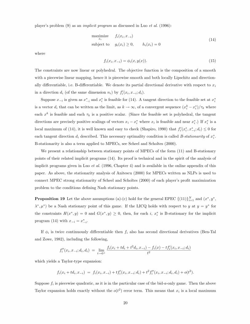
player’s problem (9) as an implicit program as discussed in Luo et al. (1996):

maximizexi

fi(xi, x−i)

subject to gi(xi) ≥ 0, hi(xi) = 0(14)

where

fi(xi, x−i) = φi(x, y(x)). (15)

The constraints are now linear or polyhedral. The objective function is the composition of a smooth

with a piecewise linear mapping, hence it is piecewise smooth and both locally Lipschitz and direction-

ally differentiable, i.e. B-differentiable. We denote its partial directional derivative with respect to xi

in a direction di (of the same dimension ni) by f ′i(xi, x−i; di).

Suppose x−i is given as x∗−i and x∗

i is feasible for (14). A tangent direction to the feasible set at x∗i

is a vector di that can be written as the limit, as k → ∞, of a convergent sequence (xki − x∗

i )/τk where

each xk is feasible and each τk is a positive scalar. (Since the feasible set is polyhedral, the tangent

directions are precisely positive scalings of vectors xi − x∗i where xi is feasible and near x∗

i .) If x∗i is a

local maximum of (14), it is well known and easy to check (Shapiro, 1990) that f ′i(x

∗i , x

∗−i; di) ≤ 0 for

each tangent direction di described. This necessary optimality condition is called B-stationarity of x∗i .

B-stationarity is also a term applied to MPECs, see Scheel and Scholtes (2000).

We present a relationship between stationary points of MPECs of the form (11) and B-stationary

points of their related implicit programs (14). Its proof is technical and in the spirit of the analysis of

implicit programs given in Luo et al. (1996, Chapter 4) and is available in the online appendix of this

paper. As above, the stationarity analysis of Anitescu (2000) for MPECs written as NLPs is used to

connect MPEC strong stationarity of Scheel and Scholtes (2000) of each player’s profit maximization

problem to the conditions defining Nash stationary points.

Proposition 19 Let the above assumptions (a)-(c) hold for the general EPEC {(11)}Ni=1 and (x∗, y∗,

λ∗, µ∗) be a Nash stationary point of this game. If the LICQ holds with respect to y at y = y∗ for

the constraints H(x∗, y) = 0 and G(x∗, y) ≥ 0, then, for each i, x∗i is B-stationary for the implicit

program (14) with x−i = x∗−i.

If φi is twice continuously differentiable then fi also has second directional derivatives (Ben-Tal

and Zowe, 1982), including the following,

f ′′i (xi, x−i; di, di) = lim

t→0+

fi(xi + tdi + t2di, x−i) − fi(x) − tf ′i(xi, x−i; di)

t2

which yields a Taylor-type expansion:

fi(xi + tdi, x−i) = fi(xi, x−i) + tf ′i(xi, x−i; di) + t2f ′′

i (xi, x−i; di, di) + o(t2).

Suppose fi is piecewise quadratic, as it is in the particular case of the bid-a-only game. Then the above

Taylor expansion holds exactly without the o(t2) error term. This means that xi is a local maximum

20

of (14) if it is B-stationary and satisfies the second-order condition that f ′′i (xi, x−i; di, di) ≤ 0 for each

feasible direction di with f ′i(xi, x−i; di) = 0. This fact is used in the proof which appears in the Online

Appendix.

5 Numerical methods and examples

We first describe the diagonalization method, which is familiar in the computational economics lit-

erature from the days of PIES energy model, Ahn and Hogan (1982), and, more recently, in Cardell

et al. (1997). Then we give computational results for randomly generated electricity market games

using both the diagonalization framework, which is implemented via standard nonlinear programming

methods, and the CP formulation of §4.3 which requires a complementarity solver.

5.1 Diagonalization method

Diagonalization is a kind of fixed-point iteration in which players cyclically or in parallel update their

strategies while treating other players’ strategies as fixed.

Diagonalization method for the game {(12)}Ni=1

(i) We are given a starting point x(0) = (x(0)1 , . . . , x

(0)N ), the maximum number of iterations K, and

a convergence tolerance ε ≥ 0.

(ii) We are given the current iterate x(k). For i = 1 to N :

Player i solves problem (12) while holding xj = zj for j < i and xj = x(k)j for j > i. Denote the

xi-part of the optimal solution by zi.

(iii) Let x(k+1) = (z1, . . . , zN ). Check convergence and stopping condition: if ‖x(k)i − x

(k−1)i ‖ < ε for

i = 1, . . . , N , then accept the point and stop; else if k < K, then increase k by one and go to (ii)

and repeat the process; else if k = K stop and output “no equilibrium point found”.

Note that the diagonalization method may fail to find a Nash equilibrium even if there exists such a

point.

In step (ii), we need an algorithm to solve the MPEC (12). There has been a lot of recent progress

in numerical methods for solving MPECs, e.g. Anitescu (2000), Fletcher et al. (2002), Hu and Ralph

(2004) and references therein, resulting in several different but apparently effective approaches. We

could simply apply an off-the-shelf NLP method to an MPEC formulated as an NLP such as (12). An

alternative is to use an iterative scheme like the regularization method, see Scholtes (2001). Regular-

ization, like the penalty (Hu and Ralph, 2004) and smoothing (Fukushima and Pang, 2000) methods,

re-models an MPEC as a one-parameter family of better-behaved nonlinear programs, and solves a

sequence of the latter while driving the parameter to zero, at which point the NLP becomes equivalent

21

to the MPEC. This leads us to call each Diagonalization iteration an outer iteration; and each iteration

within step (ii) of Diagonalization an inner iteration.

Step (ii) by regularization method (inner iteration for ith player in step (ii))

(ii-1) We are given x(k), zj for j < i, and a sequence of (typically, decreasing) regularization parame-

ters ρ(k)0 , ρ

(k)1 , . . . , ρ

(k)M , i.e. a fixed number of iterations to execute, where ρ

(k)m bounds the total

violation of complementarity in sub-iteration m. Let m = 0, ξ0i = x

(k)i .

(ii-2) Given the regularization parameter ρm, xj = zj for j < i and xj = x(k)j for j > i, and the starting

point xi = ξmi , solve the following nonlinear program

maximizexi,y,λ,µ

fi(x, y)


∇yF (x, y) −∇yG(x, y)T µ + ∇yH(x, y)T λ = 0

H(x, y) = 0

G(x, y) ≥ 0, µ ≥ 0, Gj(x, y)µj ≤ ρ(k)m , j = 1, . . . , s.

(16)

If m < M , let ξm+1i be the xi part of the solution, let m = m + 1, and repeat (ii-2).

Else let x(k+1)i be the xi part of the solution, and stop.

For m > 1, the solution values of y, λ and µ at sub-iteration m can be used, in addition to xi = ξmi ,

to initialize the corresponding variables in sub-iteration m + 1. We focus on xi however because the

other variables are assumed to be defined implicitly by it.

We give a convergence result for the diagonalization method where, at each iteration, step (ii) is

carried out using regularization. This result is essentially a corollary of the regularization convergence

analysis of Scholtes (2001) which requires that the “solution” of (16), in (ii-2), is a stationary point that

satisfies a second-order necessary condition as described in Scholtes (2001). Assuming the diagonaliza-

tion method produces a convergent subsequence, with limit (x∗i , y

∗, λ∗i , µ

∗i ) and limiting multipliers ξg

i ,

ξhi , etc as laid out in (12), a technical condition called Upper-Level Strict Complementarity, ULSC, is

needed: for each component j of µ∗i and G(x∗, y∗) such that (µ∗

i )j = Gj(x∗, y∗) = 0, neither (ξG

i )j nor

(ξµi )j is zero.

Proposition 20 Let M be fixed in (ii-1)–(ii-2) for each outer iteration k of the diagonalization method.

Assume 0 < ρ(k)M → 0. Suppose x(m) = (x

(m)i )N

i=1, satisfies the following conditions:

(i) there exist Y (m) = (y(m)i )i, λ(m) = (λ

(m)i )i and µ(m) = (µ

(m)i )i such that, for each i = 1, . . . , N ,

the tuple (x(m)i , y

(m)i , λ

(m)i , µ

(m)i ) is a stationary point satisfying a second-order necessary condi-

tion for (16) with x−i = (x(m−1)1 , . . . , x

(m−1)i−1 , x

(m−1)i+1 , . . . , x

(m−1)n );

(ii) the sequence (x(m), Y (m), λ(m), µ(m)) has a limit point (x∗, Y ∗, λ∗, µ∗) as m → ∞, where x∗ =

(x∗i )i, Y ∗ = (y∗

i )i etc.; and

22

(iii) for each i, the MPEC-LICQ and the upper level strict complementarity condition hold at (x∗i , y

∗i , λ∗

i , µ∗i )

for (12).

If y∗1 = . . . = y∗

n then the point x∗ is a Nash stationary point of game {(9)}Ni=1.

We mention that the diagonalization method presented above is a Gauss-Seidel-type scheme in

that each player updates its optimal strategy in turn, and the next player takes this into account. An

alternative is a Jacobi scheme in which, given the kth iterate x(k), each player i updates its strategy

xi based only on x(k); these updates can therefore be carried out in parallel. We describe the Jacobi

version, which would use a different step (ii).

Jacobi (ii) We are given the current iterate x(k). Each player i executes the following:

Solve problem (12) while holding x−i = x(k)−i . Denote the xi-part of the optimal solution of (12)

by x(k+1)i .

A Jacobi scheme and its convergence was discussed in Hu (2003). Further developments, including

more details of the convergence analysis supporting the above proposition, and numerical comparisons

of the Gauss-Seidel and Jacobi approaches to EPECs that favor the former, appear in Su (2004b).

5.2 Numerical examples

We give numerical results for randomly generated electricity market models in the form (2). We solve

these as EPECs in the complementarity problem formulation, see §4.3, and by applying the Gauss-

Seidel diagonalization approaches of §5.1. Comprehensive numerical testing is a subject for future work

and seems to require definition of a reasonably broad test set of problems.

We have modeled the CP formulation and two versions of the diagonalization methods using

GAMS (Brooke et al., 1992) for the bilevel game (2) over a triangular network with three bidding sce-

narios: bid-a-only, bid-b-only and bid-a-b, respectively. Our interest is in numerical behavior; see Hu

et al. (2004) for an investigation of the economic implications of equilibria computed for bid-a and

bid-b games.

The PATH solver (Dirkse and Ferris, 1995; Ferris and Munson, 1999) is used for the CP formulation.

If PATH terminates successfully, we then check the second-order sufficient condition for each player’s

MPEC. In all our successful CP tests below, we were able to establish numerically that a solution found

by PATH was indeed a local Nash equilibrium.

By Diag we mean the Gauss-Seidel diagonalization method in which each MPEC in step (ii) of

the outer iteration is formulated as an NLP, cf. (11), and solved using SNOPT (Gill et al., 2002). By

Diag/Reg we mean the Gauss-Seidel scheme using the inner iteration (ii-1)-(ii-2) described above; each

inner iteration requires solution of an NLP which is carried out using SNOPT.

The computer used to perform the computations has two 300 MHz UltraSparc II processors and

768 MB memory, and runs the Solaris operating system.

23

5.2.1 Test problems

We generate 30 random test problems based on a three-node network. The participants are one

consumer at node 1, two generators at node 2, and one generator at node 3. However, only the

generators optimize their bids while the consumer reveals its true utility function to the ISO. In this

network all lines have the same physical characteristics, which determine power flows over the network

given the injections and withdrawal of power at each node, but possibly different capacities. Node 1 is

chosen as the reference node and therefore its distribution factors are zero. The distribution factors of

node 2 to lines 12, 13, 23 are −2/3,−1/3, 1/3 respectively, and those of node 3 are −1/3,−2/3,−1/3

respectively. The transmission limits are C12 = C13 = 800.0, and C23 = 5.0.

The analysis of Section 3 suggests that equilibria are likely to exist when the lines are either largely

congested, over all feasible bids, or largely uncongested. Our numerical experience seems to confirm

this at least anecdotally. Looking ahead to Tables 1-3 we see that at least 27 out of 30 games for

each of the bid-a-only, bid-b-only and bid-a-b cases were solved by one or more of the methods tested;

looking behind these results we identified around 25 out of 30 games, for each of the three cases, in

which congestion occurred in line 23 at the solution point identified. For the discussion on the economic

effects of congestion, we refer the readers to Hu et al. (2004).

With regard to the cost coefficients Ai and Bi we note that, while quadratic cost functions are

merely stylized representations of the cost profiles faced by generators, it is accepted (Saadat, 1999)

that Bi is much smaller than Ai in the units that are commonly employed for electricity market models.

In (2), we set the bounds for the ai and bi bids as A i = 0, A i = 200.0, B i = 0.00001 and B i = 6.0.

Our test problems are generated by random selection of Ai and Bi as follows.

We use GAMS’s pseudo-random number generator (with the default seed = 3141) to generate 30

sets of uniformly distributed coefficients of generation/utility functions. The intervals over which the

random selection is made differ for each node: for the consumer at node 1, Ai and Bi are chosen in

[90.0, 120.0] and [0.2, 0.6] respectively; for the generators at node 2 the intervals are [5.0, 10.0] and

[0.01, 0.08] respectively; and, for the generator at node 3, [5.0, 20.0] and [0.01, 0.04] respectively. For

example, the consumer at node 1 has utility function A1q1 + B1q21 where A1 and B1 are chosen by

sampling uniform distributions on [90.0, 120.0] and [0.2, 0.6] respectively. However the two generators

at node 2 are provided with the same cost functions. The code checks every equilibrium outcome to

see whether both players have the same strategies; in our experiments, symmetric strategies at node 2

are verified in all cases (at least where the code converges).

The true generation cost functions are used as the starting points for all solvers.

The maximal number of outer iterations for both Diag and Diag/Reg is set to be K = 400 and

the convergence tolerance ε = 10−5 for all the problems. The norm used to check convergence of the

diagonalization schemes at iteration k is the maximum, over all player indices i, of |aki − ak−1

i |+ |bki −

bk−1i |. In the bid-a-only (bid-b-only respectively) situation, this simplifies to the maximum over i of

24

|aki − ak−1

i | ( |bki − bk−1

i | respectively).

In the inner iteration process of Diag/Reg, given any outer iteration number k, we start with

ρ(k)0 = 10−3, solve the regularized problem (16) and then divide the regularization parameter by 10.

This is repeated five times, for a total of 6 calls to SNOPT. At the end of the inner iteration process,

the maximum violation of the products of pairs of complementary scalars is 10−9.

We also introduce a tolerance for checking Nash stationarity of solutions, εstat = 10−3. For the CP

formulation, each successful termination of PATH is deemed to be Nash stationary, i.e., the violation

of the complementarity system is below 10−6 measured in the ∞-norm, which is a PATH default.

Checking Nash stationarity for solutions provided by Diag and Diag/Reg is performed by applying

PATH to the CP formulation using the solution provided as a starting point; if PATH terminates at a

point within ∞-distance εstat of the solution provided, then the latter is deemed Nash stationary.

Setting the value of εstat to be orders of magnitude larger than the PATH default stopping tolerance

allows for considerable inaccuracy in the solution provided by either of the diagonalization methods.

This is a heuristic that allows us to check the claimed success of Diag or Diag/Reg given that simple

fixed-point iteration generally does not converge faster than linearly, and therefore the termination

point has relatively low accuracy. There is, of course, the possibility that Diag or Diag/Reg may

identify a local Nash point that is not Nash stationary in which case PATH cannot confirm success.

5.2.2 Numerical results

Tables 1-3 summarize numerical results for solving 30 randomly generated models. Each model is

solved for three different game scenarios — bid-a-only, bid-b-only and bid-a-b — so we attempt to solve

90 EPECs altogether. The title of each row of data in these tables is explained next. A “convergent

problem” refers to a problem for which the algorithm in question successfully converged.

no. converged (stationary) For the CP method, this is the number of successful terminations of

PATH using its default settings. This number is repeated in the brackets since each successful

termination of PATH is associated with a Nash stationary point.

For the diagonalization methods, this is the number of problems for which fewer than K = 400

outer iterations were needed to achieve convergence of the bid sequence. The number in brackets

is the number of problems for which PATH verified Nash stationarity of the solution provided

(to within tolerance εstat explained above).

avg. CPU time The average CPU time is calculated as the total CPU time used by the solver for

all convergent problems divided by the number of such problems. For Diag and Diag/Reg the

average CPU time includes the time required for all outer and, if applicable, inner iterations (for

all convergent problems).

avg. no. outer iterations This is defined only for Diag and Diag/Reg. It is the total number of

25

outer iterations k over all convergent problems divided by the number of convergent problems.

avg. no. solver iterations This is the total number of major iterations over all convergent problems

of either PATH, for the CP formulation, or SNOPT, for the diagonalization formulations, divided

by the number of convergent problems.

In Tables 1-2, one can see both Diag and Diag/Reg successfully converge on all of the bid-a-only

and bid-b-only games, and, with only two exceptions out of 60 problems, their termination points are

verified as being approximately Nash-stationary points. For these games, applying Path to the CP

gives a solution to all but 7 problems, which is slightly less reliable than the diagonalization methods.

By contrast Table 3 shows that the bid-a-b games are very difficult for the diagonalization methods

whereas PATH is seen to be quite robust in solving all but 3 out of the 30 problem instances.

We stress that the difficulty experienced by the diagonalization methods in bid-a-b games was

not in convergence, since for the vast majority of problems these methods successfully terminated,

but in convergence to a Nash stationary point. This leaves open the question of whether or not the

diagonalization methods usually find local Nash points. If indeed a local Nash point is not Nash

stationary, then, by implication of Proposition 16, the MPEC-LICQ cannot hold there. In any event,

difficulties with most computational approaches to bid-a-b games are to be expected if, as we believe, in

contrast to the bid-a-only and bid-b-only games, the bid-a-b games have solutions that are not locally

unique; see Hu (2003, Chapter 5) for discussion on nonuniqueness of solutions. Why PATH performs

so much better than the diagonalization schemes in finding Nash stationary points of bid-a-b games is

a question for future work.

It is clear that average CPU time for the CP formulation was much less than for the diagonalization

methods, and was less affected by the type of game than the other methods. A similar statement holds

for the average number of solver iterations, shown in the last row of the tables.

CP Diag Diag/Reg

no. converged (stationary) 27 (27) 30 (28) 30 (30)

avg. CPU time 0.37 1.27 8.02

avg. no. outer iterations N/A 8 8

avg. no. solver iterations 1116 599 3652

Table 1: Comparisons of the three solution formulations for bid-a-only

26

CP Diag Diag/Reg


avg. CPU time 0.75 4.69 26.82



Table 2: Comparisons of the three solution formulations for bid-b-only

CP Diag Diag/Reg


avg. CPU time 0.14 5.86 21.38



Table 3: Comparisons of the three solution formulations for bid-a-b

6 Conclusion

Bilevel games and EPECs, unlike classical games with nonempty convex compact strategy spaces, need

not admit existence of (pure strategy) Nash equilibria under convenient general conditions. Neverthe-

less we have provided several situations in which the bilevel games considered by Berry et al. (1999),

and their EPEC counterparts, have Nash equilibria. More generally we have shown that the stationary

conditions of an EPEC can be phrased as a mixed complementarity problem whose solutions charac-

terize Nash stationary points. Computational viability of finding Nash stationary points is shown for

a class of randomly generated EPECs in the format of Berry et al. (1999). Of note is the relatively

robust and fast behavior of the PATH solver when applied to the complementarity formulation.

Acknowledgment

The authors are grateful to Eric Ralph and Stefan Scholtes for their continuing comments and en-

couragement and to anonymous referees for thoughtful suggestions that have improved the paper. We

owe special thanks to Michael Ferris and Todd Munson for providing GAMS modeling expertise; to

Michael Ferris for making available the computing environment, partly funded by US Air Force Office

of Scientific Research Grant FA9550-04-1-0192; and finally to Peter Bardsley for partial funding of this

project through a grant from the Australian Research Council.

References

Ahn, B. H. and W. W. Hogan. 1982. On convergence of the PIES algorithm for computing equilibria.

Operations Research 30, 281–300.

27

Anitescu, M. 2000. On using the elastic mode in nonlinear programming approaches to mathemati-

cal programs with complementarity constraints. Preprint, ANL/MCS-P864-1200, Mathematics and

Computer Science Division, Argonne National Laboratory, revised (2003), Argonne, Illinois, USA.

Backerman, S. R., S. J. Rassenti, and V. L. Smith. 2000. Efficiency and income shares in high

demand energy networks: who receives the congestion rents when a line is constrained? Pacific

Economic Review 5, 331–347.

Balder, E. J. 1995. A unifying approach to existence of Nash equilibria. International Journal of

Game Theory 24, 79–94.

Ben-Tal, A. and J. Zowe. 1982. A simplified theory of first and second order conditions for extreme

problems in topological vector spaces. Mathematical Programming Study 19, 39–76.

Berry, C. A., B. F. Hobbs, W. A. Meroney, R. P. O’Neill, and W. R. Stewart Jr. 1999.

Understanding how market power can arise in network competition: a game theoretic approach.

Utilities Policy 8, 139–158.

Bonnans, J. F. and A. Shapiro. 1998. Optimization problems with perturbations: A guided tour.

SIAM Review 40, 202–227.

Brooke, A., D. Kendrick, and A. Meeraus. 1992. GAMS A user’s guide, release 2.25. The

Scientific Press, South San Francisco, CA 94080-7014.

Cardell, J. B., C. C. Hitt, and W. W. Hogan. 1997. Market power and strategic interaction in

electricity networks. Resource and Energy Economics 19, 109–137.

Chao, H.-P. and S. Peck. 1997. An institutional design for an electricity contract market with

central dispatch. The Energy Journal 18, 85–110.

Clarke, F. 1993. Nonsmooth Analysis. A Wiley-Interscience Publication, New York.

David Butchers & Associates. 2001. The New Zealand electricity market (NZEM).

URL http://www.dba.org.nz/PDFs/Electricity%20Market.pdf

Dirkse, S. and M. C. Ferris. 1995. The PATH solver: A non-monotone stabilization scheme for

mixed complementarity problems. Optimization Methods and Software 5, 123–156.

Ehrenmann, A. 2004a. Equilibrium Problems with Equilibrium Constraints and their Application to

Electricity Markets. Ph.D. Dissertation, Judge Institute of Management, The University of Cam-

bridge, Cambridge, UK, Cambridge, UK.

Ehrenmann, A. 2004b. Manifolds of multi-leader Cournot equilibria. Operations Research Letters

32, 121–125.

28

Ehrenmann, A. and K. Neuhoff. 2003. A comparison of electricity market designs in networks.

working paper CMI EP 31, The CMI Electricity Project, Department of Applied Economics, The

University of Cambridge, Cambridge, UK.

Ferris, M. C. and T. S. Munson. 1999. Interfaces to PATH 3.0: Design, implementation and usage.

Computational Optimization and Applications 12, 207–227.

Fletcher, R. and S. Leyffer. 2004. Solving mathematical program with complementarity con-

straints as nonlinear programs. Optimization Methods and Software 19, 15–40.

Fletcher, R., S. Leyffer, D. Ralph, and S. Scholtes. 2002. Local convergence of SQP meth-

ods for mathematical programs with equilibrium constraints. Numerical Analysis Report NA 209,

Department of Mathematics, University of Dundee, Dundee, UK.

Fukushima, M. and J.-S. Pang. 2000. Convergence of a smoothing continuation method for math-

ematical programs with complementarity constraints. In Thera, M. and R. Tichatschke (eds.),

Ill-posed Variational Problems and Regularization Techniques. Springer, pp. 99–110.

Gill, P., W. Murray, and M. Sanders. 2002. SNOPT 6.0 .

URL http://www.sbsi-sol-optimize.com/asp/sol product snopt.htm

Green, R. J. and D. M. Newbery. 1992. Competition in the British electricity spot market. Journal

of Political Economy 100, 929–953.

Hobbs, B. F., C. B. Metzler, and J.-S. Pang. 2000. Strategic gaming analysis for electric power

systems: an MPEC approach. IEEE Transactions on Power Systems 15, 637–645.

Hogan, W. 1992. Contract networks for electric power transmission. Journal of Regulatory Economics

4, 211–242.

Hu, X. 2003. Mathematical Programs with Complementarity Constraints and Game Theory Models

in Electricity Markets. Ph.D. thesis, Department of Mathematics and Statistics, The University of

Melbourne, Parkville, Victoria, Australia.

Hu, X. and D. Ralph. 2001. Nash equilibria for games in competitive electricity markets under

network constraints. In Li, D. (ed.), Proceedings of ICOTA 2001, 5th International Conference on

Optimization: Techniques and Applications. University of Hong Kong, Hong Kong.

Hu, X. and D. Ralph. 2004. Convergence of a penalty method for mathematical programming with

complementarity constraints. Journal of Optimization Theory and Applications 123, 365–390.

Hu, X., D. Ralph, E. Ralph, P. Bardsley, and M. Ferris. revised 2004. Electricity genera-

tion with looped transmission networks: bidding to an ISO. working paper CMI EP 65, The CMI

29

Electricity Project, Department of Applied Economics, The University of Cambridge, Cambridge,

UK.

Klemperer, P. D. and M. A. Meyer. 1989. Supply function equilibria in oligopoly under uncer-

tainty. Econometrica 57, 1243–1277.

Leyffer, S. and T. Munson. 2005. Solving Multi-Leader-Follower Games. Preprint, ANL/MCS-

P1243-0405, Mathematics and Computer Science Division, Argonne National Laboratory, Argonne,

Illinois, USA.

Liu, M. and G. Gross. 12004. Role of distribution factors in congestion revenue rights applications.

IEEE Transactions on Power Systems 19, 802–810.

Luo, Z. Q., J.-S. Pang, and D. Ralph. 1996. Mathematical Programs with Equilibrium Constraints.

Cambridge University Press, Cambridge, UK.

Murphy, F. and Y. Smeers. 2002. Generation capacity expansion in imperfect competitive re-

structured electricity markets. Discussion Paper 2002/69, CORE, Universite catholique de Louvain,

Louvain-la-Neuve, Belgium.

Myerson, R. B. 1991. Game Theory: Analysis of Conflict. Harvard University Press, Cambridge,

Massachusetts.

Nasser, T.-O. 1998. Transmission congestion contracts and strategic behavior in generation. The

Electricity Journal 11, 32–39.

Oren, S. S. 1997. Economic inefficiency of passive transmission rights in congested electricity systems

with competitive generation. The Energy Journal 18, 63–83.

Outrata, J. 2003. A note on a class of equilibrium problems with equilibrium constraints. Kybernetika

40, 585–594.

Ralph, D. 1994. Global convergence of Newton’s method for nonsmooth equations, via the path

search. Mathematics of Operations Research 19, 352–389.

Robinson, S. M. 1994. Newton’s method for a class of nonsmooth functions. Set-Valued Analysis 2,

291–305.

Saadat, H. 1999. Power Systems. McGraw-Hill, Boston, Massachusetts, USA.

Scheel, M. and S. Scholtes. 2000. Mathematical programs with complementarity constraints:

Stationarity, optimality, and sensitivity. Mathematics of Operations Research 25, 1–22.

Scholtes, S. 2001. Convergence properties of a regularization scheme for mathematical programs

with complementarity constraints. SIAM Journal on Optimization 11, 918–936.

30

Scholtes, S. and M. Stohr. 2001. How stringent is the linear independence assumption for mathe-

matical programs with stationarity constraints? Mathematics of Operations Research 21, 851–863.

Seeley, K., J. Lawarree, and C. C. Liu. 2000. Analysis of electricity market rules and their effects

on strategic behaviour in a noncongestive grid. IEEE Transactions on Power Systems 15, 157–162.

Shapiro, A. 1990. On concepts of directional differentiability. Journal of Optimization Theory and

Applications 66, 477–487.

Stoft, S. 1999. Financial transmission rights meet Cournot: how TCCs curb market power. Energy

Journal 20, 1–23.

Su, C.-L. 2004a. Analysis on forward market equilibrium model. manuscript, Department of Man-

agement Science and Engineering, Stanford University, Stanford, California.

Su, C.-L. 2004b. A sequential NCP algorithm for solving equilibrium problems with equilibrium

constraints. manuscript, Department of Management Science and Engineering Stanford University,

Stanford, California.

Weber, J. and T. J. Overbye. 1999. A two-level optimization problem for analysis of market

bidding strategies. In IEEE PES Summer Meeting in Edmonton, Canada.

Wood, A. J. and B. F. Wollenberg. 1996. Power Generation, Operation, and Control. John-Wiley

& Sons, Inc, New York.

Wu, F. and P. Varaiya. 1997. Coordinated multilateral trades for electric power networks: theory

and implementation. POWER Working Papers PWP-031, University of California Energy Institute,

California.

Xian, W., L. Yuzeng, and Z. Shaohua. 2004. Oligopolistic equilibrium analysis for electricity

markets: a nonlinear complementarity approach. IEEE Transactions on Power Systems 19, 1348–

1355.

Yao, J., I. Adler, and S. Oren. 2005. Modeling and computing two-settlement oligopolistic equilib-

rium in a congested electricity network. Manuscript, Department of IEOR, University of California,

Berkeley, California.

Younes, Z. and M. Ilic. 1999. Generation strategies for gaming transmission constraints: will the

deregulated electric power market be an oligopoly? Decision Support Systems 24, 207–222.

31

On line appendix

Proof of Proposition 3 Let C denote the (closed convex) feasible set of (1). Lemma 1 gives the

existence of the solution q∗(a) of (1). The usual optimality conditions for convex programs say that

the gradient of the objective function of (1) at q∗(a) satisfies

[a + 2Qq∗(a)]T (c − q∗(a)) ≥ 0, for all c ∈ C.

For another value of a, call it a′, the optimal q is q∗(a′) ∈ C. Taking c = q∗(a′) above gives

[a + 2Qq∗(a)]T (q∗(a′) − q∗(a)) ≥ 0.

Exchanging a and a′ by symmetry,

[a′ + 2Qq∗(a′)]T (q∗(a) − q∗(a′)) ≥ 0.

Adding terms in the last two inequalities, we have

[a − a′ + 2Q(q∗(a) − q∗(a′))]T (q∗(a′) − q∗(a)) ≥ 0.

Hence

(a − a′)T (q∗(a′) − q∗(a)) ≥ 2(q∗(a) − q∗(a′))T Q(q∗(a) − q∗(a′)) ≥ 0 (17)

where nonnegativity follows because Q is a diagonal matrix with positive diagonal entries (or, more

generally, Q is positive definite).

If a′j = aj for each j 6= i, then

(a − a′)T (q∗(a′) − q∗(a)) = (ai − a′i)(q

∗i (a′) − q∗i (a)). (18)

So, (17) implies that (ai − a′i)(q

∗i (a′) − q∗i (a)) ≥ 0, which means that q∗i (·, a−i) is a non-increasing

function in ai.

In addition, note that Q is a diagonal matrix with ith diagonal element Bi > 0, hence (q∗(a) −

q∗(a′))T Q(q∗(a) − q∗(a′)) ≥ (q∗i (a) − q∗i (a′))2Bi. From (17) and (18) we get

|q∗i (a) − q∗i (a′)| ≤ |ai − a′i|/2Bi,

i.e., q∗(·, a−i) is Lipschitz of modulus 1/2Bi. The required bound on the directional derivative follows.

And the estimate of the set of generalized gradients follows directly from its definition. �

Proof of Theorem 4 Define X(a−i) = {ai ∈ Ai : fi(ai, a−i) ≥ 0}, X+(a−i) = {ai ∈ Ai :

fi(ai, a−i) > 0}, and X−(a−i) = {ai ∈ Ai : fi(ai, a−i) < 0}. Let participant i be a generator in

the proof; a similar proof holds for a consumer node. Let a−i be fixed. Recall the payoff function

fi(ai) = [ai − Ai + Biq∗i (ai, a−i)]q

∗i (ai, a−i) from (3). Using Proposition 3, we see that the direc-

tional derivative of the mapping ai 7→ ai − Ai + Biq∗i (ai, a−i) in the direction u = 1 is bounded

32

below by 1/2, i.e. the mapping is increasing in ai. As q∗i (ai, a−i) ≥ 0 is a non-increasing function

in ai by Proposition 3, the set X−(a−i) is an intersection of two open intervals in R. So the set

X(a−i) = Ai \X−(a−i) is a closed interval of Ai. It is nonempty since Ai is a feasible bid by assump-

tion and fi(Ai) = Biq∗i (Ai, a−i)

2 ≥ 0. Similarly, the set X+(a−i) is an open, possibly empty, interval

in Ai.

If X+(a−i) = ∅, then fi(ai, a−i) = 0 for any ai ∈ X(a−i). In this case, fi(ai, a−i) is concave in

ai ∈ X(a−i). So, assume that X+(a−i) 6= ∅.

Let w1, . . . , wW be the breakpoints of the derivative of q∗i (·, a−i). The concavity of fi(·, a−i) in

(wj , wj+1) follows from the negative semidefiniteness of its Hessian, that is,

fi′′ = 2(1 + Biq

∗i′)q∗i

′ ≤ 0, (19)

where fi′′ is the second derivative of fi(·, a−i), which follows from Proposition 3. Note that (19) implies

that the derivative fi′ of fi(·, a−i) is nonincreasing between any two consecutive breakpoints. Now we

check the concavity of fi(·, a−i) near a breakpoint wj such that fi(wj , a−i) > 0. By inequality (5), we

have the following inequality:

limv↑wj

fi′(v, a−i) = lim

v↑wj

[

q∗i (v, a−i) +(

v − Ai + 2Biq∗i (v, a−i)

)

q∗i′(v, a−i)

]

≥ limv↓wj

[q∗i (v, a−i) +(

v − Ai + 2Biq∗i (v, a−i)

)

q∗i′(v, a−i)] = lim

v↓wj

fi′(v, a−i)

(20)

since wj − Ai + 2Biq∗i (wj , a−i) > wj − Ai + Biq

∗i (wj , a−i) > 0 by the positive profit condition.

Inequality (20) implies that the (generalized) gradient of fi(·, a−i) is non-increasing near wj . There-

fore, fi(·, a−i) is concave on X+(a−i) and is quasi-concave on the nonempty closed interval X(a−i).

By Theorem 2, the game {(4)}Ni=1 has at least one Nash equilibrium. �

Proof of Proposition 16 Statement (i) ⇒ statement (ii): Write π = (µ, λ) and π∗ = (µ∗, λ∗). Fix

i and x−i = x∗−i. For any neighborhood Ui of (x∗

i , y∗) there exists a neighborhood Vi of (x∗

i , y∗, π∗)

such that (xi, y, π) ∈ Vi implies (xi, y) ∈ Ui, and the corresponding value of objective function of the

MPEC (11) coincides with that of the bilevel game (9). It is therefore clear that (x∗, y∗, π∗) is a local

Nash point of the EPEC if (x∗, y∗) is a local Nash point of the bilevel program.

Statement (ii) ⇒ statement (iii): This relies on a combination of standard MPEC stationary con-

ditions using MPEC-LICQ, e.g., Scheel and Scholtes (2000), and work relating these to stationary

conditions for NLP formulations of MPECs, Anitescu (2000). �

Proof of Theorem 18 Recall we are dealing with the implicit programming formulation {(4)}Ni=1 of

the bid-linear-only electricity market game, with EPEC reformulation {(13)}Ni=1. From Proposition 16,

the LICQ condition for (1) at q = q∗ with a = a∗ means that a local Nash equilibrium of the former

game is equivalent to a local Nash equilibrium of the latter EPEC. That is, statements (i) and (ii) of

the theorem are equivalent.

Let fi be player i’s objective function, (3). From Proposition 19 we have that a∗i is B-stationary

for Player i’s problem (4). Furthermore, since fi(·, a∗−i) is piecewise quadratic, from previous remarks

33

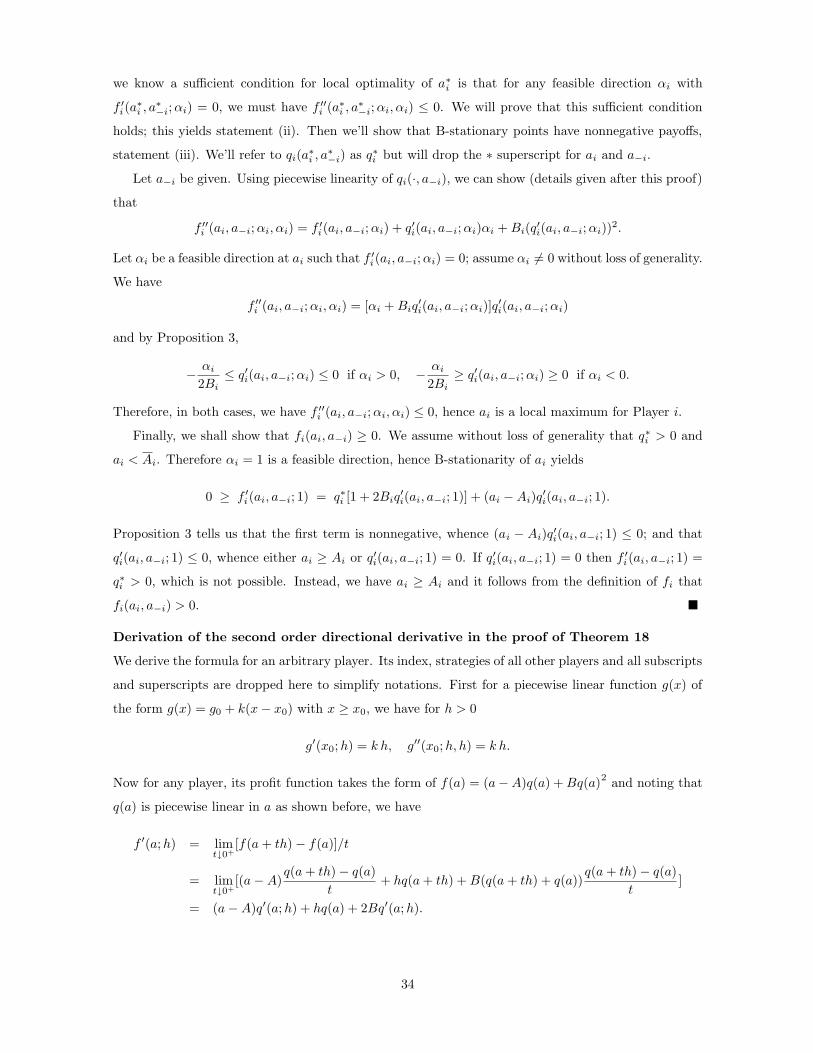
we know a sufficient condition for local optimality of a∗i is that for any feasible direction αi with

f ′i(a

∗i , a

∗−i;αi) = 0, we must have f ′′

i (a∗i , a

∗−i;αi, αi) ≤ 0. We will prove that this sufficient condition

holds; this yields statement (ii). Then we’ll show that B-stationary points have nonnegative payoffs,

statement (iii). We’ll refer to qi(a∗i , a

∗−i) as q∗i but will drop the ∗ superscript for ai and a−i.

Let a−i be given. Using piecewise linearity of qi(·, a−i), we can show (details given after this proof)

that

f ′′i (ai, a−i;αi, αi) = f ′

i(ai, a−i;αi) + q′i(ai, a−i;αi)αi + Bi(q′i(ai, a−i;αi))

2.

Let αi be a feasible direction at ai such that f ′i(ai, a−i;αi) = 0; assume αi 6= 0 without loss of generality.

We have

f ′′i (ai, a−i;αi, αi) = [αi + Biq

′i(ai, a−i;αi)]q

′i(ai, a−i;αi)

and by Proposition 3,

−αi

2Bi

≤ q′i(ai, a−i;αi) ≤ 0 if αi > 0, −αi

2Bi

≥ q′i(ai, a−i;αi) ≥ 0 if αi < 0.

Therefore, in both cases, we have f ′′i (ai, a−i;αi, αi) ≤ 0, hence ai is a local maximum for Player i.

Finally, we shall show that fi(ai, a−i) ≥ 0. We assume without loss of generality that q∗i > 0 and

ai < Ai. Therefore αi = 1 is a feasible direction, hence B-stationarity of ai yields

0 ≥ f ′i(ai, a−i; 1) = q∗i [1 + 2Biq

′i(ai, a−i; 1)] + (ai − Ai)q

′i(ai, a−i; 1).

Proposition 3 tells us that the first term is nonnegative, whence (ai − Ai)q′i(ai, a−i; 1) ≤ 0; and that

q′i(ai, a−i; 1) ≤ 0, whence either ai ≥ Ai or q′i(ai, a−i; 1) = 0. If q′i(ai, a−i; 1) = 0 then f ′i(ai, a−i; 1) =

q∗i > 0, which is not possible. Instead, we have ai ≥ Ai and it follows from the definition of fi that

fi(ai, a−i) > 0. �

Derivation of the second order directional derivative in the proof of Theorem 18

We derive the formula for an arbitrary player. Its index, strategies of all other players and all subscripts

and superscripts are dropped here to simplify notations. First for a piecewise linear function g(x) of

the form g(x) = g0 + k(x − x0) with x ≥ x0, we have for h > 0

g′(x0;h) = k h, g′′(x0;h, h) = k h.

Now for any player, its profit function takes the form of f(a) = (a − A)q(a) + Bq(a)2

and noting that

q(a) is piecewise linear in a as shown before, we have

f ′(a;h) = limt↓0+

[f(a + th) − f(a)]/t

= limt↓0+

[(a − A)q(a + th) − q(a)

t+ hq(a + th) + B(q(a + th) + q(a))

q(a + th) − q(a)

t]

= (a − A)q′(a;h) + hq(a) + 2Bq′(a;h).

34

Therefore the second order directional derivative is given by

f ′′(a;h, h) = limt↓0+

[f(a + th + t2h) − f(a) − tf ′(a;h)]/t2

= limt↓0+

[(a − A)q(a + th + t2h) − q(a) − tq′(a;h)

t2+ h

q(a + th) − q(a)

t+ hq(a + th + t2h)

+ Bq(a + th + t2h)2 − q(a)2 − 2tq(a)q′(a;h)

t2]

= (a − A)q′(a;h) + hq′(a;h) + hq(a)

+ B limt↓0+

(q(a + th + t2h) + q(a))q(a + th + t2h) − q(a) − tq′(a;h)

t2

+ Bq′(a;h) limt↓0+

q(a + th + t2h) − q(a)

t

= (a − A + 2B)q′(a;h) + q(a)h + q′(a;h)h + Bq′(a;h)2

= f ′(a;h) + q′(a;h)h + Bq′(a;h)2

which establishes the formula for the second order parabolic directional derivative of fi used in the

proof of Theorem 18. �

Proof of Proposition 19 Let (x∗, y∗, λ∗, µ∗) be Nash stationary with the LICQ holding as described

above. Consider player i’s MPEC with x−i = x∗−i. According to Anitescu (2000), since (x∗

i , y∗, λ∗, µ∗)

is stationary for the corresponding NLP (12), then it is strongly stationary for the MPEC (11) in the

terminology of Scheel and Scholtes (2000). Strong stationarity implies what is called B-stationarity of

the MPEC which is expressed in terms of a linearization of the problem about the point (x∗i , y

∗, λ∗, µ∗);

again see Scheel and Scholtes (2000). Since the constraint functions of the MPEC are already affine,

linearizing these functions is redundant and we can express B-stationarity using the tangent cone T to

the feasible set at (x∗i , y

∗, λ∗, µ∗), that is

∇xi,yφi(x∗, y∗)(di, dy) ≤ 0 for each d = (di, dy, dλ, dµ) ∈ T . (21)

This is a basic stationarity condition for the MPEC discussed in generality in Luo et al. (1996, §3.1);

it is implied by B-stationarity under smooth rather than affine constraint functions, and is equivalent

to B-stationarity under linear constraint functions or other constraint qualifications.

Next suppose di lies in the tangent cone of the feasible set {xi : gi(xi) ≥ 0, hi(xi) = 0} of the

implicit program (14) at x∗i . This feasible set is exactly the upper-level feasible set for (11) and

is polyhedral. This means x∗i + τdi is upper-level feasible for all small τ > 0. Now use piecewise

smoothness of (y(x), λ(x), µ(x)) to obtain the following partial directional derivatives:

(

y′i(x

∗; di), λ′i(x

∗; di), µ′i(x

∗; di))

= limτ↓0

(

y(x∗i + τdi), λ(x∗

i + τdi), µ(x∗i + τdi)

)

− (y∗, λ∗, µ∗)

τ.

That is, (di, y′i(x

∗; di), λ′i(x

∗; di), µ′i(x

∗; di)) belongs to T .

Finally we have for any di, from first principles or by using a chain rule Shapiro (1990), that

f ′i(x

∗i , x

∗−i; di) = ∇xi,yφi(x

∗, y∗)(di, y′i(x

∗; di)).

35

With this, the above tangent cone relationship and the MPEC B-stationary condition (21), the result

follows. �

36

Using EPECs to Model Bilevel Games in Restructured ... EPECs to Model Bilevel Games in Restructured...

Documents

Transcript of Using EPECs to Model Bilevel Games in Restructured ... EPECs to Model Bilevel Games in Restructured...