AB HELSINKI UNIVERSITY OF TECHNOLOGYFACULTY OF INFORMATION AND NATURAL SCIENCESDEPARTMENT OF COMPUTER SCIENCE AND ENGINEERING

Using Delaunay Triangulation in

Infrastructure Design Software

Master’s Thesis

Ville Herva

Department of Computer Science and Engineering

Espoo 2009

ii

AB TEKNILLINEN KORKEAKOULUINFORMAATIO- JA LUONNONTIETEIDEN TIEDEKUNTATIETOTEKNIIKAN LAITOS

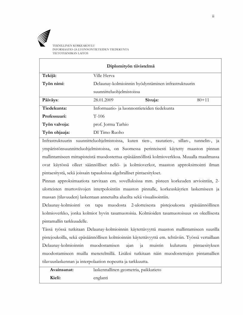
Diplomityön tiivistelmä

Tekijä: Ville Herva

Työn nimi: Delaunay-kolmioinnin hyödyntäminen infrastruktuurin

suunnitteluohjelmistoissa

Päiväys: 28.01.2009 Sivuja: 80+11

Tiedekunta: Informaatio- ja luonnontieteiden tiedekunta

Professuuri: T-106

Työn valvoja: prof. Jorma Tarhio

Työn ohjaaja: DI Timo Ruoho

Infrastruktuurin suunnitteluohjelmistoissa, kuten tien-, rautatien-, sillan-, tunnelin-, ja

ympäristönsuunnitteluohjelmistoissa, on Suomessa perinteisesti käytetty maaston pinnan

mallintamiseen mittapisteistä muodostettua epäsäännöllistä kolmioverkkoa. Muualla maailmassa

ovat käytössä olleet säännölliset neliö- ja kolmioverkot, maaston approksimointi ilman

pintaesitystä, sekä joissain tapauksissa algebralliset pintaesitykset.

Pinnan approksimaatiota tarvitaan em. sovelluksissa mm. pisteen korkeuden arviointiin, 2-

ulotteisten murtoviivojen interpolointiin maaston pinnalle, korkeuskäyrien laskemiseen ja

massan (tilavuuden) laskentaan annetuilta alueilta sekä visualisointiin.

Delaunay-kolmiointi on tapa muodosta 2-ulotteisesta pistejoukosta epäsäännöllinen

kolmioverkko, jonka kolmiot hyvin tasamuotoisia. Kolmioiden tasamuotoisuus on oleellisesta

pintamallin tarkkuudelle.

Tässä työssä tutkitaan Delaunay-kolmioinnin käytettävyyttä maaston mallintamiseen suurilla

pistejoukoilla, sekä epäsäännöllisen kolmioinnin käytettävyyttä em. tehtäviin. Työssä vertaillaan

Delaunay-kolmioinnin muodostamisen ajan ja muistin kulutusta pintaesityksen

muodostamiseen muilla menetelmillä. Lisäksi tutkitaan näin muodostettujen pintamallien

tilavuuslaskennan ja interpolaation nopeutta ja tarkkuutta.

Avainsanat: laskennallinen geometria, paikkatieto

Kieli: englanti

iii

AB HELSINKI UNIVERSITY OF TECHNOLOGYFACULTY OF INFORMATION AND NATURAL SCIENCESDEPARTMENT OF COMPUTER SCIENCE AND ENGINEERING

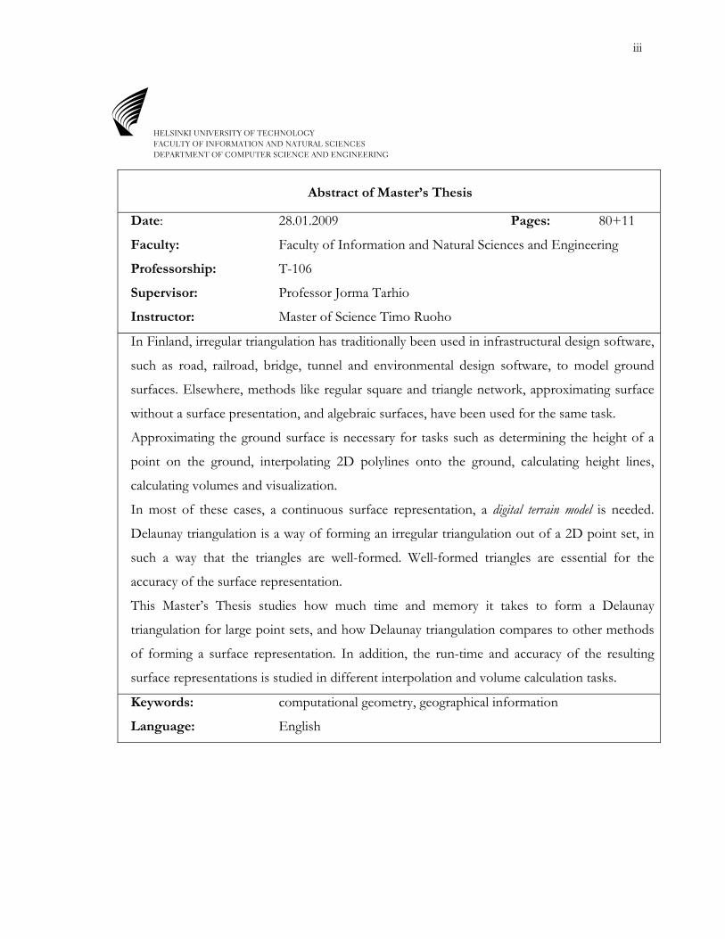
Abstract of Master’s Thesis

Date: 28.01.2009 Pages: 80+11

Faculty: Faculty of Information and Natural Sciences and Engineering

Professorship: T-106

Supervisor: Professor Jorma Tarhio

Instructor: Master of Science Timo Ruoho

In Finland, irregular triangulation has traditionally been used in infrastructural design software,

such as road, railroad, bridge, tunnel and environmental design software, to model ground

surfaces. Elsewhere, methods like regular square and triangle network, approximating surface

without a surface presentation, and algebraic surfaces, have been used for the same task.

Approximating the ground surface is necessary for tasks such as determining the height of a

point on the ground, interpolating 2D polylines onto the ground, calculating height lines,

calculating volumes and visualization.

In most of these cases, a continuous surface representation, a digital terrain model is needed.

Delaunay triangulation is a way of forming an irregular triangulation out of a 2D point set, in

such a way that the triangles are well-formed. Well-formed triangles are essential for the

accuracy of the surface representation.

This Master’s Thesis studies how much time and memory it takes to form a Delaunay

triangulation for large point sets, and how Delaunay triangulation compares to other methods

of forming a surface representation. In addition, the run-time and accuracy of the resulting

surface representations is studied in different interpolation and volume calculation tasks.

Keywords: computational geometry, geographical information

Language: English

iv

Table of Contents

Table of Contents ......................................................................................................................................................... iv Terminology and Abbreviations ................................................................................................................................ vi List of Figures ............................................................................................................................................................... ix List of Diagrams ............................................................................................................................................................ x List of Tables .................................................................................................................................................................. x 0 ............................................................................................................................................................. xi Foreword

1 ......................................................................................................................................................... 1 Introduction

2 .............................................................................................................................................. 4 Problem Statement

2.1 ............................................................................................................................................... 4 Scope of Thesis

2.2 ........................................................................................................ 5 Triangulation of an Irregular Point Set

2.2.1 ............................................................................................................................ 7 Arbitrary Triangulation

2.2.2 .................................................................................................................... 8 Quality of the Triangulation

2.2.3 ............................................................................................................................ 9 Delaunay Triangulation

2.2.4 .......................................................................................................................................... 11 Other Criteria

2.3 ................................................................................................................................ 13 Alternative Approaches

2.3.1 ........................................................................................... 13 Regular Grid (Rectangular) Triangulation

2.3.2 ........................................................................ 14 Bézier surfaces and Non-uniform B-Spline surfaces

2.3.3 ..................................................................................................................... 15 Direct Point Interpolation

3 ............................................................................................ 18 Infrastructure Design Software and Workflow

3.1 ....................................................... 20 Input Data Considerations for the Infrastructure Design Process

3.2 ............................................................................................................................ 21 Quality of the Input Data

4 ................................................................................................................................. 22 Triangulation Algorithms

4.1 .................................................................................................................................. 22 Algorithms Categories

4.1.1 .............................................................................................................................. 22 Sweepline Algorithm

4.1.2 ............................................................................................................ 23 Divide-and-conquer Algorithm

4.1.3 ........................................................................................................................ 25 Radial Sweep Algorithm

4.1.4 .......................................................................................................................... 27 Step-by-step Algorithm

4.1.5 ........................................................................................................................... 28 Incremental Algorithm

4.1.6 ............................................................................................................ 31 Convex Hull Based Algorithms

4.1.7 ..................................................................................................................................... 32 Specialized Cases

4.2 .................................................................................................. 32 Point Data Triangulation with Fold-lines

4.2.1 .................................................................................................................................. 34 Other Approaches

4.2.2 ........................................................................................................................... 34 Additional Constraints

v

5 ..................................................................................... 35 Manipulating and Using an Existing Triangulation

5.1 ............................................................................................................................................... 35 Adding a Point

5.2 .................................................................................................................................. 36 Adding a Set of Points

5.3 ............................................................................................................................................. 36 Deleting a Point

5.4 ................................................................................................................................ 37 Deleting a Set of Points

5.5 ................................................................................................................ 37 Folding with a Line or a Polyline

5.6 ...................................................................................................................... 38 Simplifying the Triangulation

5.7 ....................................................................................................... 39 Artificially Refining the Triangulation

5.8 ............................................................................................ 41 Interpolating a Height Value for a 2D Point

5.9 ............................................................................................................... 43 Interpolating a Line or a Polyline

5.10 ....................................................................................................................................... 44 Calculating Volume

6 ...................................................................................................................... 45 Implementation Considerations

6.1 ............................................................................................. 45 Robustness of the Triangulation Algorithm

6.2 .............................................................................................................................................. 47 Data Structures

6.3 .............................................................................................................................................. 48 Multi-threading

6.4 .............................................................................................................. 49 Non-General Purpose Processors

7 ............................................................................................................. 50 The Implementation and Evaluation

7.1 ..................................................................................................................................... 50 The Implementation

7.1.1 ........................................................................................................................................ 50 Data Structures

7.1.2 ........................................................................................................................ 53 Triangulation Algorithm

7.1.3 ............................................................................................................................... 54 Complexity Analysis

7.1.4 ....................................................................................................................... 55 Interpolation Algorithms

7.1.5 ............................................................................................................. 55 Volume Calculation Algorithm

7.2 .................................................................................................................................................. 56 Environment

7.3 ....................................................................... 58 Evaluation of the Implementation against Other DTMs

7.3.1 ............................................................................................................................................. 58 Sample Data

7.3.2 ............................................................................................................... 62 Other Digital Terrain Models

7.3.3 ................................................................................................................................................... 63 Run-time

7.3.4 ................................................................................................... 66 Accuracy in Interpolation of a Point

7.3.5 ............................................................................................... 68 Accuracy in Interpolation of a Polyline

7.3.6 .......................................................................................................... 69 Accuracy in Volume Calculation

7.3.7 ......................................................................................................................................... 72 Previous Work

8 .......................................................................................................................................................... 73 Conclusion

References ..................................................................................................................................................................... 75

vi

Terminology and Abbreviations

2D Two-dimensional (usually x and y coordinates)

3D Three-dimensional

CAD Computer-aided Design

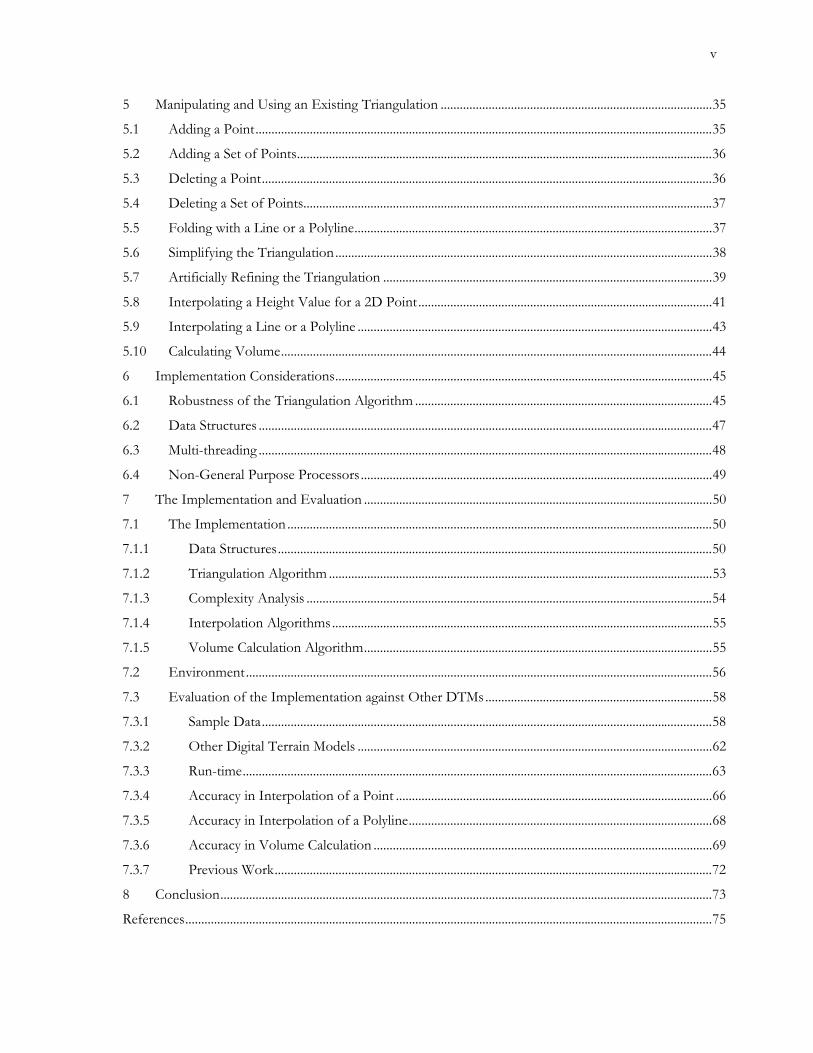
Delaunay criterion A triangle in a TIN fulfills the Delaunay criterion if no other points

than the three triangle vertices lie inside the circle drawn via the

three vertices. The circle is called the Delaunay neighborhood of the

triangle.

Triangle that

satisfies the

Delaunay criterion

A non-Delaunay triangle

since there is an extra point

in the Delaunay

neighborhood

Figure: Delaunay criterion

Delaunay triangulation A TIN is a Delaunay triangulation if and only if all of its triangles

satisfy the Delaunay criterion. A Delaunay triangulation for a given

set of points is unique, unless there are triangle-pairs where both

middle-edge alternatives give two Delaunay fulfilling triangles.

DTM (Digital Terrain Model) Numerical model of the measured (or planned) terrain surface.

Edge-neighbor A triangle that shares and edge (and two vertices) with another

triangle.

Edge-swap A triangle-pair has four non-common edges, and one common edge

(middle-edge). For fixed four non-common edges, the middle-edge

can be chosen in two ways. Edge-swap is an operation on triangle-

pair that changes the middle-edge from one alternative to the other.

Fold-line A line via which the edges of a TIN are forced to go

GIS Geographic Information System

Middle-edge The common edge in a triangle-pair.

vii

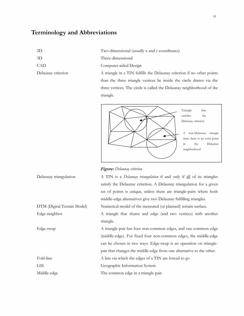
Min-max criterion Min-max criterion (minimum-maximum) says that in a triangle-pair,

the middle-edge should be chosen so that the largest angle of all six

angles in the triangle-pair is as small as possible.

configuration A configuration B

αB1

αA1 αA2

αB2

αA3

αB3 comparison value =

max(αA1,2,3,αB1,2,3)

αB3

αB1

αB2

αA1

αA3

αB2

Figure: Min-max criterion

Point-neighbor A triangle that shares one or two points with another triangle.

Quad-edge See Triangle-pair

Tachymeter A tachymeter or tacheometer is a kind of theodolite used for

geographic measurements. It measures, optically or electronically,

the distance to target. Tachymeters are often used in surveying.

Having accurately measured the lengths and angles of the sides of

triangles in a triangle network or chain, the shape of the ground can

be calculated.

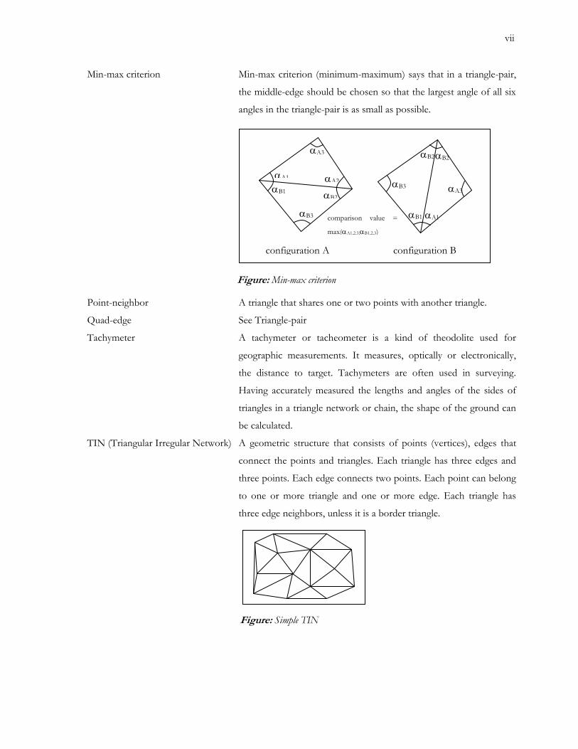
TIN (Triangular Irregular Network) A geometric structure that consists of points (vertices), edges that

connect the points and triangles. Each triangle has three edges and

three points. Each edge connects two points. Each point can belong

to one or more triangle and one or more edge. Each triangle has

three edge neighbors, unless it is a border triangle.

Figure: Simple TIN

viii

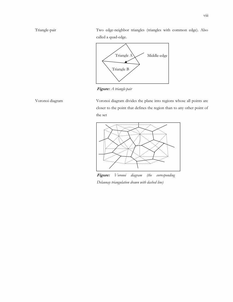
Triangle-pair Two edge-neighbor triangles (triangles with common edge). Also

called a quad-edge.

Triangle A Middle-edge

Triangle B

Figure: A triangle-pair

Voronoi diagram Voronoi diagram divides the plane into regions whose all points are

closer to the point that defines the region than to any other point of

the set

Figure: Voronoi diagram (the corresponding

Delaunay triangulation drawn with dashed line)

ix

List of Figures

1.1 Interpolating a point from a set of measured points 3

2.1 An overhang where an x, y point has three different z values 6

2.2 Perspective view of a TIN 7

2.3 Intuitive triangulation retains the form of the ridge 9

2.4 A different triangulation would obviously produce dubious results for point interpolation 9

2.5 A Delaunay triangulation with one non-Delaunay triangle pair 10

2.6 A Voronoi diagram 11

2.7 A T-junction 12

2.8 A regular triangulation from the same data as in Figure 2.2 13

2.9 Interpreting point data as matrix 14

2.10 Regular triangulation 14

4.1 Divide-and-conquer algorithm: Merge step 24

4.2 Radial sweep algorithm: Initial edges sorted by their angles 26

4.3 Radial sweep algorithm: Triangles formed between the edges 26

4.4 Radial sweep algorithm: Non-convex notches filled 26

4.5 Radial sweep algorithm: Triangulation is refined to satisfy Delaunay-criterion 26

4.6 Step-by-step algorithm: Initial base line is chosen and the first apex is sought 28

4.7 Step-by-step algorithm: New edges are appended to edges-to-do stack 28

4.8 Incremental algorithm: An initial triangulation is formed 30

4.9 Incremental algorithm: Points are inserted to the triangulation one by one 30

4.10 Incremental algorithm: While inserting the points, the Delaunay criterion is maintained 30

4.11 Incremental algorithm: After inserting all the points, we have a Delaunay triangulation 30

4.12 Incremental algorithm: The triangulation is made convex again 31

7.1 The reference surface 58

7.2 Sample point set for N=5000 60

7.3 The Delaunay triangulation of sample point set from Figure 7.2 61

7.4 The real world data set from Vuotos area 62

7.5 Comparing regular grid triangulation to the Delaunay triangulation of the point set 63

7.6 Comparing the intersections from Delaunay triangulation and regular grid triangulation 69

7.7 The sample Delaunay triangulation from Figure 7.3 compared to z=0 70

x

List of Diagrams

7.1 The run-time of the two methods 64

7.2 The point interpolation error of the two methods 66

7.3 Comparing the interpolation accuracy with real world data 68

List of Tables

7.1 The run-time of interpolation and volume calculation 65

7.2 The volume calculation results of the two methods 71

7.3 The volume difference calculation results of the two methods 72

xi

0 Foreword

This Master’s Thesis has been made in the end of year 2008 and beginning of 2009 in Vianova Systems

Finland Oy. I would like to thank development manager Timo Ruoho for allowing me to work on this

thesis at Vianova.

Vianova Systems Finland is an inspiring place to work, but what was miraculous was that there was also

serene enough atmosphere to concentrate on such a long-term work. This wouldn’t have been possible

without Vianova’s help in arranging the projects so that there was a long quiet period to work on the

thesis. I also wish to thank all my colleagues and Vianova Systems Finland.

Delaunay triangulation, its mathematical background and its good characteristics in the practical

applications are an interesting subject. The whole area of computational geometry is somewhat

underrepresented in the current computer science education. I hope in future more people will find this

area interesting.

Espoo January 12th 2009

Ville Herva

1

1 Introduction

Before design projects such as road, railroad, building and environment designs can be started, the

affected area needs to be surveyed. This process involves measuring the locations of existing buildings,

delves and other stationary objects. Most importantly, the shape, consistency and composition of the

surface must be surveyed. Consistency and composition is usually measured by drilling samples off the

soil. The volumetric distribution of different soil types is then interpolated between the sample drill points

[PP98].

The shape of the surface is measured with methods such as tachymeters, GPS and aerial photographs (see

section 3.1). The data these methods yield is arbitrary point data − a large number of points on the surface

whose X, Y and Z coordinates are known accurately. Often, it is assumed that the surface is 2.5-

dimensional – that is, for a given 2-dimensional location (x, y) there is only one point (x, y, z) that lies on

the surface. Depending on the method used, the number of sample points on a given area can vary wildly.

Also, the accuracy and type of error of sample points varies [Nur02].

Because the survey raw survey data only consists of a set of points that lie on the surface, a method of

constructing an approximation of the actual surface is needed. Without a representation of the surface,

such tasks as calculating Z of given (x, y) or calculating height line for given Z, cannot be carried out. It is

clear that we need a continuous representation of the surface that is defined for every point (x, y) on the

area.

In infrastructure design, this representation is usually referred to as Digital Terrain Model (DTM). First

digital terrain models date back to 1958 (due to Massachusetts Institute of Technology professor Charles

Miller), but they became popular in commercial infrastructure design in the 1980’s. Closely related term to

DTM is Digital Elevation Model (DEM). In digital elevation model, there is a height value for each two-

dimensional point either in the form of a height matrix or a raster file or a there is a mean to calculate the

height from the DEM [HD06].

Before we can decide what kind of a representation we should choose, we will have to know the

operations we will use the representation for. For a typical civil engineering project, these operations

include

2

• Interpolating heights for arbitrary points on the area

• Solving the 2D-polyline that is the intersection of the surface representation and a XY-plane on a

given height (the height line)

• Computing the volume between the volume between the surface representation and a XY-plane

on a given height on a given XY-area

• Computing the volume between the volume between the surface representation and the

representation of another surface on a given XY-area

• Computing the intersection of between the surface representation and objects such as 3D-line,

3D-plane or another surface representation

• Visualization: polygon rendering, ray-tracing etc.

These are the most common applications [HHKL09]. In specialized tasks, digital terrain models are used

for calculation the flow of water, estimating the visibility, calculating noise propagation and so on. These

uses of DTM pose their own requirements for the surface representation, but they are outside of the

scope of this thesis.

Although we only know the height of the terrain where we have measured it, not anywhere else,

interpolating a height for a point can be easily accomplished for almost any kind of surface representation.

However, additional requirements are often posed for this operation. For example, it is often required that

when interpolating the height for a point from the representation in a measured point, the result must be

the measured height. This makes a lot of sense, since the measured points are the only ones we know the

height at. However, this excludes some popular variations of curved surfaces, such as Bézier surfaces.

Other requirement might be that when interpolating points on a 2D-path, there may not be

discontinuations (that is, when the 2D-distance of two sample points approaches zero, the height

difference does not approach zero). If the surface representation satisfies this criterion, it is said to be

(first order) continuous. Sometimes even second order continuousness (the derivative of the surface is

continuous) is desired. In most cases, the height can be accurately solved – that is, a direct algebraic

solution exists [BKOS97].

3

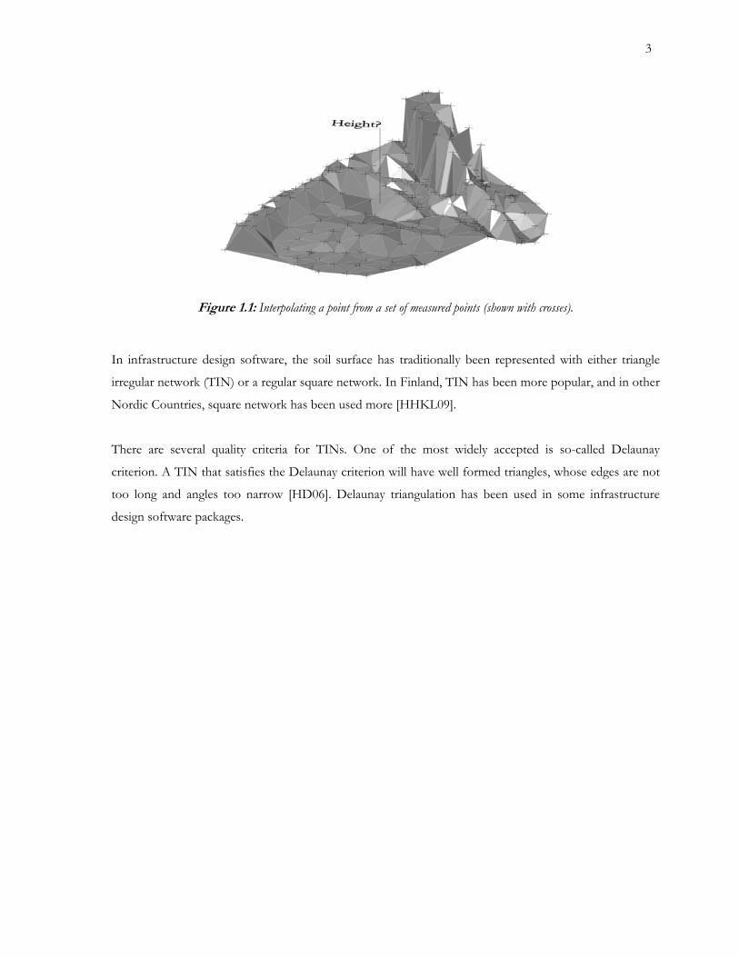
Figure 1.1: Interpolating a point from a set of measured points (shown with crosses).

In infrastructure design software, the soil surface has traditionally been represented with either triangle

irregular network (TIN) or a regular square network. In Finland, TIN has been more popular, and in other

Nordic Countries, square network has been used more [HHKL09].

There are several quality criteria for TINs. One of the most widely accepted is so-called Delaunay

criterion. A TIN that satisfies the Delaunay criterion will have well formed triangles, whose edges are not

too long and angles too narrow [HD06]. Delaunay triangulation has been used in some infrastructure

design software packages.

4

2 Problem Statement

2.1 Scope of Thesis

In this thesis, I intend to study the algorithms for creating, updating and using Delaunay triangulation in

infrastructure design applications. I will compare Delaunay triangulation to other alternatives based on the

following criteria:

• accuracy

• robustness (whether the method is prone to special cases where the results are unpredictable)

• runtime

• memory use

• simplicity of implementation

For infrastructure design application, the following operations are crucial:

• creating the surface representation

• updating the surface representation (deleting and adding points)

• interpolating heights of 2D points and polylines

• calculating volumes.

To evaluate how suitable Delaunay triangulation is for infrastructure design application, I will implement

these operations for Delaunay triangulation and chosen alternative surface representations. Based on their

popularity in current infrastructure design software packages, I have chosen regular grid triangle network

and direct interpolation from the point data as the competing surface representations.

I will compare the accuracy and run-time with both ideal sample data (whose accurate form in known) and

real-world data. Because real-world data is measured only at sample sites, the true formation of the surface

is represents is not known. This makes it somewhat harder to draw reliable conclusions of the accuracy of

the methods. However, with certain procedures which I will present later, some conclusions can be draw.

I will also discuss algorithms to implement Delaunay triangulation from point data and point data with

fold-lines. I will describe in more detail the algorithm I chose to implement and comment its run-time and

memory use compared to others.

5

2.2 Triangulation of an Irregular Point Set

A planar map is a topological map on a 2D plane. It divides the plane into faces that consist of edges that

define their boundary. Thus, a face is a polygon. The edges are line segments that begin from the origin

vertex and end at destination vertex (although the direction of the edge is not important for all

applications.) For a planar map to be complete, each edge should be neighbored by two faces, unless it is a

boundary edge for the whole planar map. Each vertex must be connected to one or more edges and no

edges may cross.

Forming a planar map of a surface described by a given point set is a common way to represent the

surface in continuous manner. When forming the planar map, we consider the point set as 2D – that is,

the z coordinate does not affect the shape of the planar graph – but we maintain the z coordinate as an

attribute that can later be used for the interpolation and volume calculation operations.

We can form a planar map using however complex polygons as faces as we please. If one looks at the

world map, one can consider the countries (and the sea) as very complex polygons, and the map is thus a

planar map (ignoring the spherical projection). However, when modeling the terrain surface, the points

carry the height information as well, and the planar map is actually not planar. In order for the

interpolation and volume calculation operations to have well-defined results, the polygons need to be

planar. For polygons with four or more three-dimensional vertices this is a special case, but for a triangle,

this constraint is always met. On the other hand, any polygon with more than three vertices can always be

divided into triangles. This is why it is common to use triangles only as the faces of the planar map.

A planar map with triangles as faces and 3D vertices is called a triangulation or a TIN (triangle irregular

network.) A triangulation is a maximal planar subdivision of a point set, because no edges can be added to it

so that it would still be a planar map.

A triangulation can be formed out of any 2D point set given that is not degenerated - that is, not all points

are identical nor collinear. In practical applications, all identical points are discarded, and if any points

have the same x, y but not z it is considered an error in the input data. The point set is said to be 2.5D: for

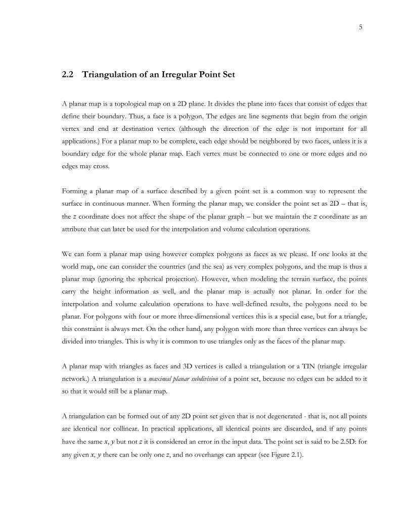
any given x, y there can be only one z, and no overhangs can appear (see Figure 2.1).

6

Figure 2.1: An overhang where an x, y point has three different z values.

In planar map, a face that only has boundary edges is called an unbounded face. Likewise, a combination of

faces that form an area, whose boundaries compose of boundary edges, is called an unbounded face. For a

complete planar map the only unbounded face is the union of all faces, and its boundary edges form the

convex hull of the point set. A face whose all edges are non-boundary edges is a bounded face. Such face is

surrounded by other face from all sides.

The process of forming a TIN out of a point set is called triangulating it, and the result is called a

triangulation. There are several possible triangulations for a given point set (given that is has more than 3

points.) However, all these triangulations have the same amount of vertices, edges and triangles. The

count of triangles can be derived from the Euler’s formula. Take a point set p with n points. Its convex

hull is unambiguous. Let us denote the number of points in p that lie on the convex hull with k. Any

triangulation of p then has 2n – 2 – k triangles and 3n – 3 – k edges [BKOS97]. Note that the convex hull

can be expressed with fewer vertexes than k if some of the points that lie on the convex hull are collinear.

For these formulae, k needs to include the collinear points as well.

7

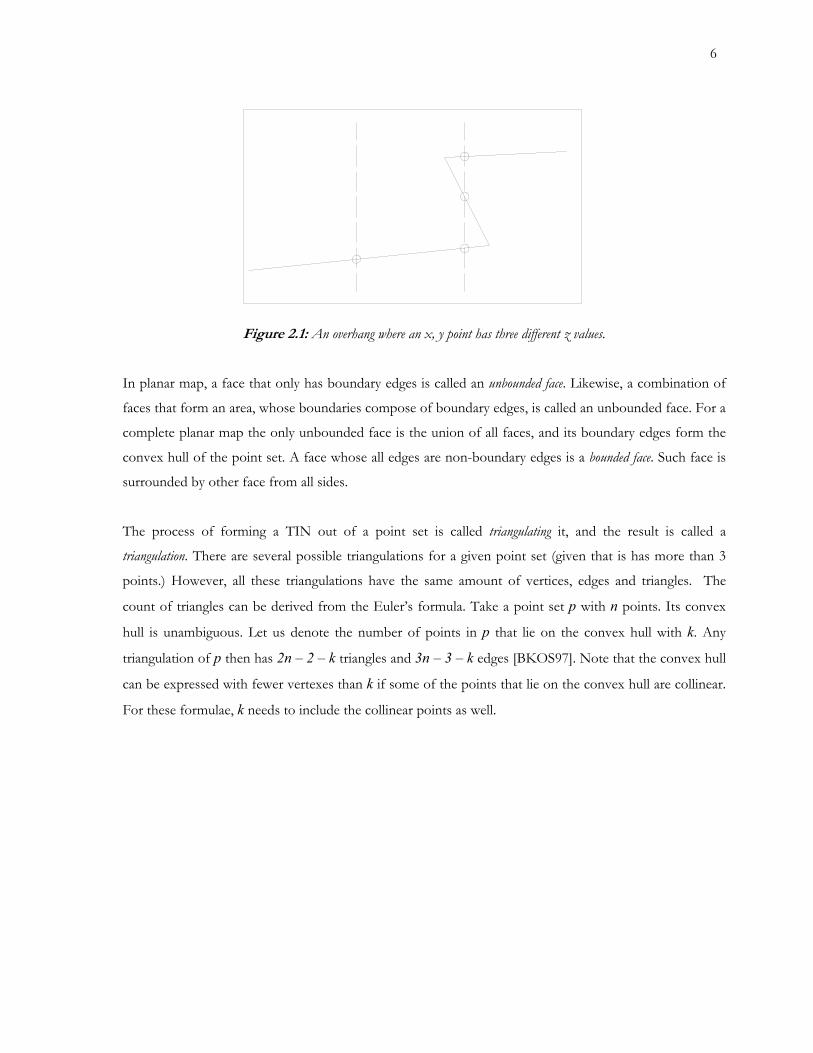
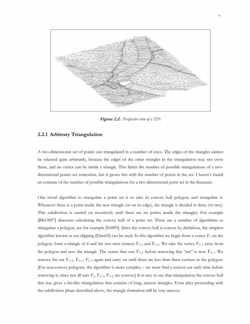
Figure 2.2: Perspective view of a TIN

2.2.1 Arbitrary Triangulation

A two-dimensional set of points can triangulated in a number of ways. The edges of the triangles cannot

be selected quite arbitrarily, because the edges of the other triangles in the triangulation may not cross

them, and no vertex can be inside a triangle. This limits the number of possible triangulations of a two-

dimensional points set somewhat, but it grows fast with the number of points in the set. I haven’t found

an estimate of the number of possible triangulations for a two-dimensional point set in the literature.

One trivial algorithm to triangulate a point set is to take its convex hull polygon, and triangulate it.

Whenever there is a point inside the new triangle (or on its edge), the triangle is divided in three (or two).

This subdivision is carried on recursively until there are no points inside the triangles. For example

[BKOS97] discusses calculating the convex hull of a point set. There are a number of algorithms to

triangulate a polygon, see for example [NM95]. Since the convex hull is convex by definition, the simplest

algorithm known as ear-clipping [Eber02] can be used. In this algorithm we begin from a vertex Vi on the

polygon, form a triangle of it and the two next vertices Vi+1 and Vi+2. We take the vertex Vi+1 away from

the polygon and save the triangle. The vertex that was Vi+2 before removing this “ear” is now Vi+1. We

remove the ear Vi+1, Vi+1, Vi+2 again and carry on until there are less than three vertices in the polygon.

[For non-convex polygons, the algorithm is more complex – we must find a convex ear each time before

removing it, since not all ears Vi, Vi+1, Vi+2 are convex.] It is easy to see that triangulation the convex hull

this way gives a fan-like triangulation that consists of long, narrow triangles. Even after proceeding with

the subdivision phase described above, the triangle formation will be very uneven.

8

2.2.2 Quality of the Triangulation

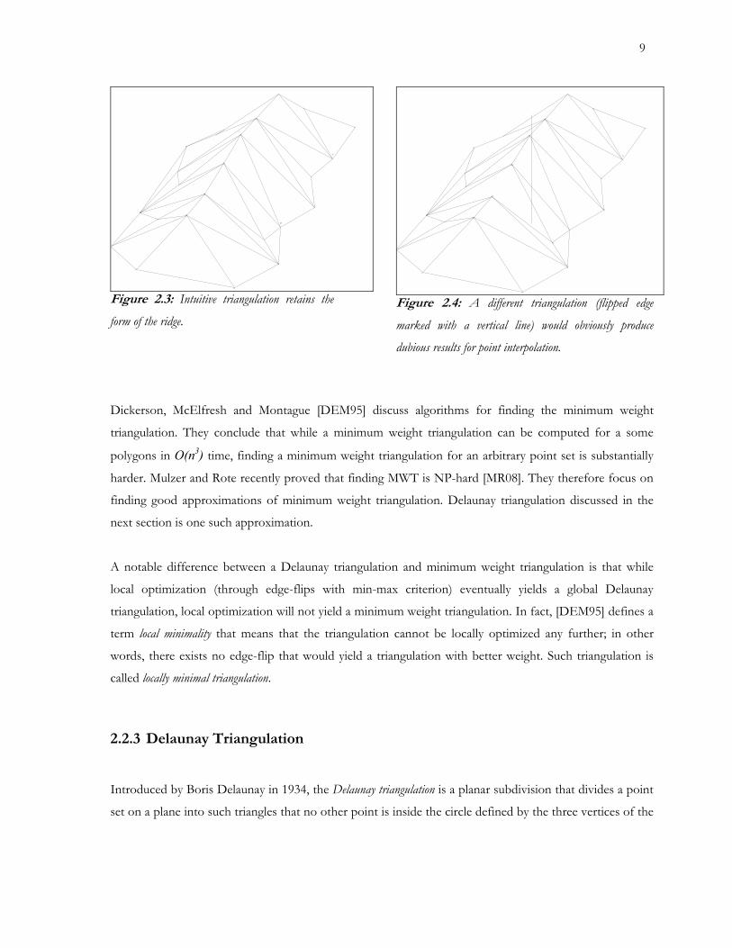
The quality of the triangulation is defined by how well it approximates the real surface – i.e. how well

heights interpolated from it correspond to the real height, and how well volumes calculated from it

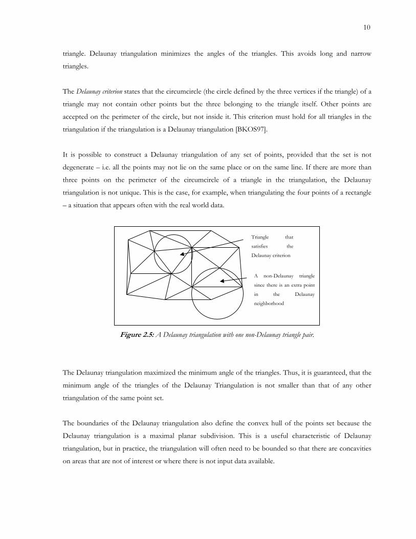
correspond to the real volumes. Consider the two TINs in Figures 2.3 and 2.4. They model a real ground

surface that has a ridge. Both are triangulated from measured sample points. The difference between the

two triangulations is the two triangles between the four vertices in marked by vertical line in Figure 2.4.

Those four points can be triangulated in two ways: like in Figure 2.3 or like in Figure 2.4. In theory, the

real ground surface could resemble either of the two, but it is much more likely to resemble the one in

Figure 2.3. The question is: how do we make sure the triangulation we have is most likely to resemble the

surface it approximates.

It turns out that a triangulation most likely to resemble the approximated surface has as short triangle

sides as possible. This minimizes the distance to the vertices from any given point on the triangle. Because

the vertices are the known heights of the real surface, and the real surface is likely to have similar height

near the measured points, the points used for interpolation (the triangle vertices) should be selected near

the interpolated point.

One alternative for finding and optimal triangulation is to minimize the sum of the lengths of the edges in

the triangulation. A triangulation that has the lowest possible sum of the lengths of the edges is called the

minimum weight triangulation (MWT) of a point set. The sum of lengths of the edges of a triangulation is

called the weight of a triangulation.

9

Figure 2.3: Intuitive triangulation retains the

form of the ridge.

Figure 2.4: A different triangulation (flipped edge

marked with a vertical line) would obviously produce

dubious results for point interpolation.

Dickerson, McElfresh and Montague [DEM95] discuss algorithms for finding the minimum weight

triangulation. They conclude that while a minimum weight triangulation can be computed for a some

polygons in O(n )3 time, finding a minimum weight triangulation for an arbitrary point set is substantially

harder. Mulzer and Rote recently proved that finding MWT is NP-hard [MR08]. They therefore focus on

finding good approximations of minimum weight triangulation. Delaunay triangulation discussed in the

next section is one such approximation.

A notable difference between a Delaunay triangulation and minimum weight triangulation is that while

local optimization (through edge-flips with min-max criterion) eventually yields a global Delaunay

triangulation, local optimization will not yield a minimum weight triangulation. In fact, [DEM95] defines a

term local minimality that means that the triangulation cannot be locally optimized any further; in other

words, there exists no edge-flip that would yield a triangulation with better weight. Such triangulation is

called locally minimal triangulation.

2.2.3 Delaunay Triangulation

Introduced by Boris Delaunay in 1934, the Delaunay triangulation is a planar subdivision that divides a point

set on a plane into such triangles that no other point is inside the circle defined by the three vertices of the

10

triangle. Delaunay triangulation minimizes the angles of the triangles. This avoids long and narrow

triangles.

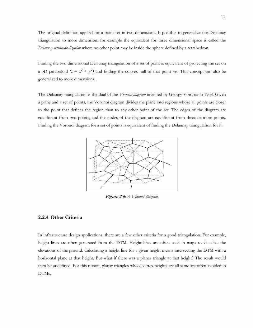
The Delaunay criterion states that the circumcircle (the circle defined by the three vertices if the triangle) of a

triangle may not contain other points but the three belonging to the triangle itself. Other points are

accepted on the perimeter of the circle, but not inside it. This criterion must hold for all triangles in the

triangulation if the triangulation is a Delaunay triangulation [BKOS97].

It is possible to construct a Delaunay triangulation of any set of points, provided that the set is not

degenerate – i.e. all the points may not lie on the same place or on the same line. If there are more than

three points on the perimeter of the circumcircle of a triangle in the triangulation, the Delaunay

triangulation is not unique. This is the case, for example, when triangulating the four points of a rectangle

– a situation that appears often with the real world data.

Figure 2.5: A Delaunay triangulation with one non-Delaunay triangle pair.

The Delaunay triangulation maximized the minimum angle of the triangles. Thus, it is guaranteed, that the

minimum angle of the triangles of the Delaunay Triangulation is not smaller than that of any other

triangulation of the same point set.

The boundaries of the Delaunay triangulation also define the convex hull of the points set because the

Delaunay triangulation is a maximal planar subdivision. This is a useful characteristic of Delaunay

triangulation, but in practice, the triangulation will often need to be bounded so that there are concavities

on areas that are not of interest or where there is not input data available.

Triangle that

satisfies the

Delaunay criterion

A non-Delaunay triangle

since there is an extra point

in the Delaunay

neighborhood

11

The original definition applied for a point set in two dimensions. It possible to generalize the Delaunay

triangulation to more dimension; for example the equivalent for three dimensional space is called the

Delaunay tetrahedralization where no other point may be inside the sphere defined by a tetrahedron.

Finding the two dimensional Delaunay triangulation of a set of point is equivalent of projecting the set on

a 3D paraboloid (z = x + y )2 2 and finding the convex hull of that point set. This concept can also be

generalized to more dimensions.

The Delaunay triangulation is the dual of the Voronoi diagram invented by Georgy Voronoi in 1908. Given

a plane and a set of points, the Voronoi diagram divides the plane into regions whose all points are closer

to the point that defines the region than to any other point of the set. The edges of the diagram are

equidistant from two points, and the nodes of the diagram are equidistant from three or more points.

Finding the Voronoi diagram for a set of points is equivalent of finding the Delaunay triangulation for it.

Figure 2.6: A Voronoi diagram.

2.2.4 Other Criteria

In infrastructure design applications, there are a few other criteria for a good triangulation. For example,

height lines are often generated from the DTM. Height lines are often used in maps to visualize the

elevations of the ground. Calculating a height line for a given height means intersecting the DTM with a

horizontal plane at that height. But what if there was a planar triangle at that height? The result would

then be undefined. For this reason, planar triangles whose vertex heights are all same are often avoided in

DTMs.

12

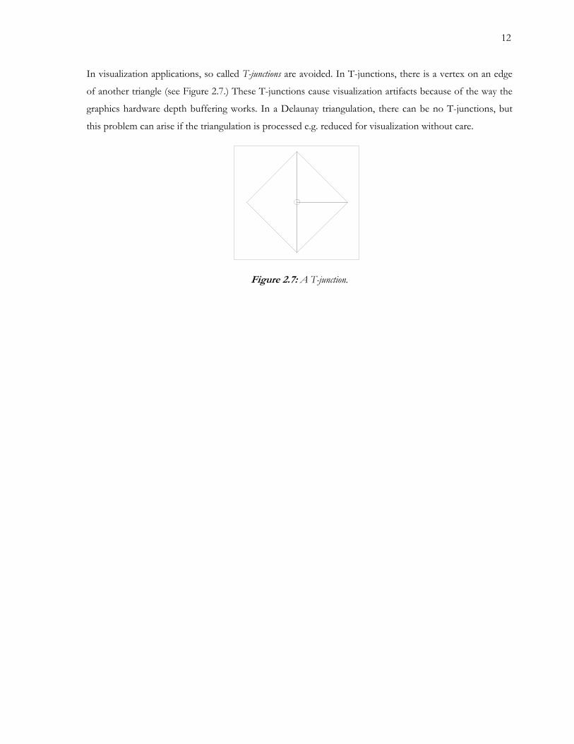
In visualization applications, so called T-junctions are avoided. In T-junctions, there is a vertex on an edge

of another triangle (see Figure 2.7.) These T-junctions cause visualization artifacts because of the way the

graphics hardware depth buffering works. In a Delaunay triangulation, there can be no T-junctions, but

this problem can arise if the triangulation is processed e.g. reduced for visualization without care.

Figure 2.7: A T-junction.

13

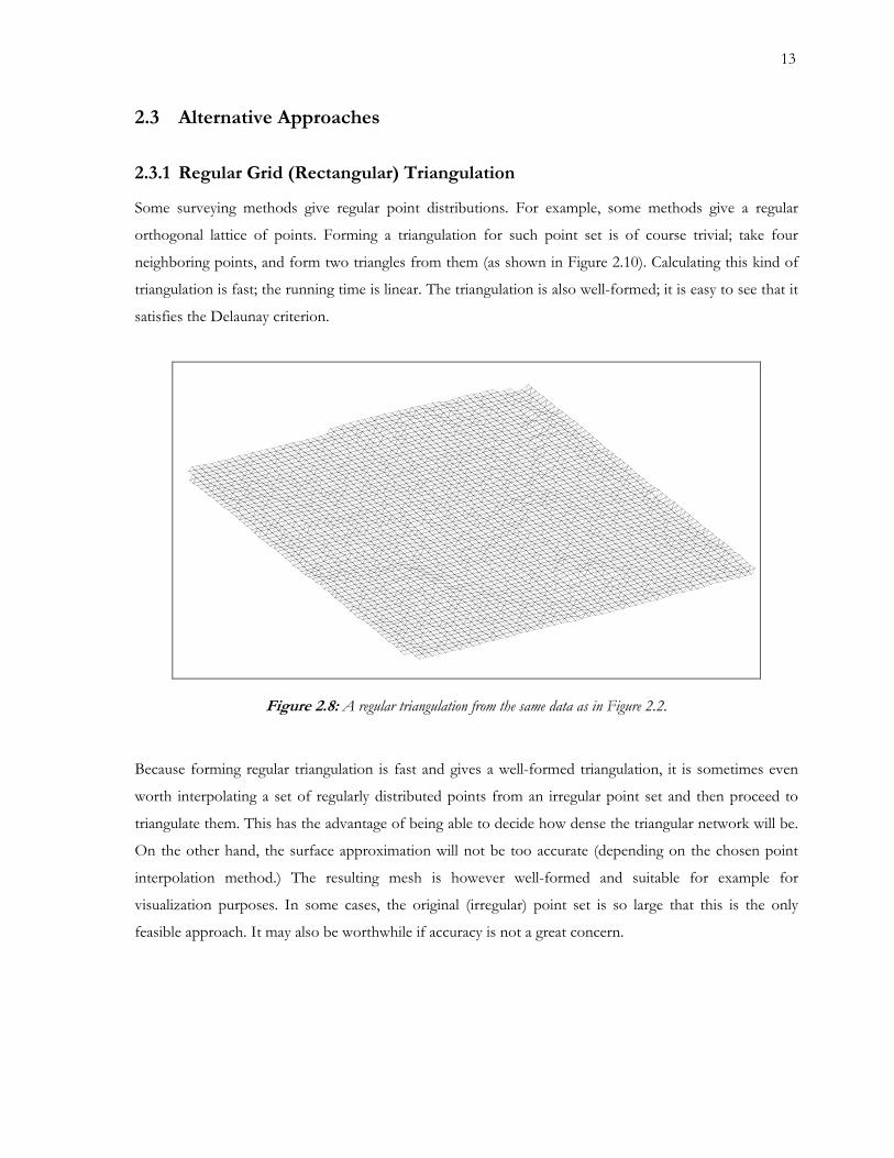
2.3 Alternative Approaches

2.3.1 Regular Grid (Rectangular) Triangulation

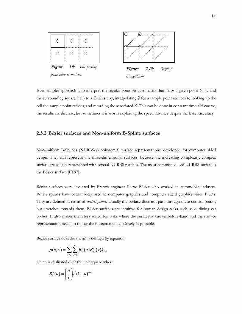
Some surveying methods give regular point distributions. For example, some methods give a regular

orthogonal lattice of points. Forming a triangulation for such point set is of course trivial; take four

neighboring points, and form two triangles from them (as shown in Figure 2.10). Calculating this kind of

triangulation is fast; the running time is linear. The triangulation is also well-formed; it is easy to see that it

satisfies the Delaunay criterion.

Figure 2.8: A regular triangulation from the same data as in Figure 2.2.

Because forming regular triangulation is fast and gives a well-formed triangulation, it is sometimes even

worth interpolating a set of regularly distributed points from an irregular point set and then proceed to

e the triangular network will be.

n the other hand, the surface approximation will not be too accurate (depending on the chosen point

triangulate them. This has the advantage of being able to decide how dens

O

interpolation method.) The resulting mesh is however well-formed and suitable for example for

visualization purposes. In some cases, the original (irregular) point set is so large that this is the only

feasible approach. It may also be worthwhile if accuracy is not a great concern.

14

lar point set as a matrix that maps a given point (x, y) and

the surrounding square (cell) to a Z. This way, interpolating Z for a sample point reduces to looking up the

cell the sample point resides, and returning the associated Z. This can be done in constant time. Of course,

.3.2 Bézier surfaces and Non-uniform B-Spline surfaces

ns, developed for computer aided

esign. They can represent any three-dimensional surfaces. Because the increasing complexity, complex

ézier surfaces were invented by French engineer Pierre Bézier who worked in automobile industry.

human design tasks such as outlining car

odies. It also makes them less suited for tasks where the surface is known before-hand and the surface

representation needs to follow the measurement as closely as possible.

ézier surface of order (n, m) is defined by equation

Even simpler approach is to interpret the regu

the results are discrete, but sometimes it is worth exploiting the speed advance despite the lesser accuracy.

2

Non-uniform B-Splines (NURBSes) polynomial surface representatio

d

surface are usually represented with several NURBS patches. The most commonly used NURBS surface is

the Bézier surface [PT97].

B

Bézier splines have been widely used in computer graphics and computer aided graphics since 1980’s.

They are defined in terms of control points. Usually the surface does not pass through these control points,

but stretches towards them. Bézier surfaces are intuitive for

b

B

jimj

n

i

m

j

ni kvBuBvup ,

0 0)()(),( ∑∑

= =

=

which is evaluated over the unit square where

inini uu

in

uB −−⎟⎟⎠

⎞⎜⎜⎝

⎛= )1()(

Figure 2.9: Interpreting

point data as matrix. Figure 2.10: Regular

triangulation.

15

is a Bernstein polynomial. [HLS93] This gives us the position of point p as function of coordinates u and

zier surfaces are generally formed out of multiple simpler

ézier patches (Bézier surfaces of small order) that are fitted together.

he strong point of Bézier surfaces is their smoothness with relatively small computational overhead. This

c

.3.3 Direct Point Interpolation

t is not strictly necessary to have a representatio of the surface to carry out certain tasks. For example,

interpolating Z for a given (x, y) can be easily accomplished based solely on the point data. However, tasks

for a given Z, or calculating the volume between two surfaces, while perhaps

not impossible to accomplish without a mathematical representation of the surface, are usually done using

surface representation.

nterpolating a point from a set of points is quite straightforward and can be carried out in O(log N) time

o interpolate Z for a given p = (x, y) from a set of points

, the most intuitive approach is to search n nearest points (denote them with R = p1…n) from the point

ata, and then calculate the average Z of p1...n.

v. A Bézier surface of order (m, n) will have n + 1 times m + 1 control points.

Bézier surface can be of any order, but as we can see from the equation, the calculation burden quickly

grows heavier as the order rises, and large Bé

B

For example Gálvez, Iglesias, Cobo, Puig-Pey and Espinola [GICPE07] describe algorithms to fit Bézier

surfaces to follow 3D point sets as optimally as possible, but the algorithms for this are nowhere near as

simple as for TINs and square networks.

T

is particularly useful in omputer graphics. I am unaware of any widely used infrastructure design program

that uses Bézier surfaces as soil ground surface representation.

2

I n

such as solving height line

a

I

(or even faster, depending of desired accuracy). T

P

d

The n points (assuming n is constant) can be found in logarithmic time, given that the point set P is sorted

or otherwise organized to a suitable data structure. Even sorting the points by X (and if X is equal, Y) and

then using binary search gives logarithmic running time. More sophisticated methods such a spatial

hashing [THMPG03], or quadtree [BKOS97] can give even better running time, but the performance is

rarely a concern unless n is very large and a large number of points is interpolated.

16

The average of Z of p1...n can be weighted to get better accuracy. A common method is to weight the pi in

e sum with the inverse distance or inverse quadratic distance from p to pi. The sum equation then th

becomes

∑∑ ⋅

=

ii

i ip

p ppdistppdist

zz

i

),(),(

1

or, for quadratic distance

∑∑ ⋅

=

ii

i ip

pppdist

zz

i 2),(1

ppdist 2),(

where dist(p , p ) is the distance on XY

1 2 -plane or

221

22121 )()(),( yyxxppdist −+−=

Choosing suitable n is not easy. One approach is to choose a distance d, and take all the points from P

whose dist(p, p ) < di rather than n nearest points. However, the density of the points can vary over the

area, and just blindly choosing a d that appears sensible for most of the data could yield no points at all on

certain areas. On the other hand, always taking n points farthest of which can be very far away makes no

more sense. However, weighting the result with the inverse distance (or, moreover, inverse square

distance) ensures that if such far-away points appear among p1...n their contribution to the result is

negligible.

Unless the result is weighted with inverse distance, this method suffers from discontinuations. Let us

assume we are interpolating a 2D line l onto the surface that the point set P approximates. We do this by

sampling points from the line and interpolating their Z from P. The resulting 3D polyline is the mapping

of l on the surface approximated by P. In theory, the more we interpolate points (and the smaller their

distance is) the better the result is. However, just taking the average Z of p1…n means that two sample

points that are infinitely near each other can have significant difference in their interpolated Z. This is

because the points (and thus, their contribution to the result) discretely appear and disappear from the

17

point set included in the sum. This problem can be seen with the weighted average as well (unless n = nP),

but it is much smaller.

he solution would be to choose the points that are nearer than the maximum distance d, and weight their

T

contribution so that for points whose dist(p, pi) ≥ d have zero contribution and point (if any) whose

dist(p, pi) = 0 has infinite contribution. The contribution of points whose d ≥ dist(p, pi) ≥ 0 could be

chosen to be linear or quadratic. This way, the new points that appear in the point set begin to affect

smoothly (as do the points that disappear from the set). However, it is difficult or impossible to choose

the d so that the point set always contains enough points, and on the other hand never contains too many

points (which ruins the running time of the algorithm.)

18

3 Infrastructure Design Software and Workflow

The term Infrastructure Design Software refers to Civil engineering applications that are used to design,

odel and maintain infrastructural objects, such as roads, railroads, bridges, tunnels, dams, airports,

he infrastructure design software suites are often built on top of more general Computer Aided Design

nstrained by laws, regulations,

ngineering guidelines and best practices that vary from country to country. Also, designing different

ngineering an infrastructure with a modern infrastructure design software package is really a computer

ted that these advantages in the design process give more than ten-fold increase in

productive in come cases [HHKL09].

The process of designing, construction and maintaining an infrastructure has several phases. For example,

road design process consists of pre-design, general design and construction design phases. After that,

computers are used in the construction and maintenance phases. In some cases, a different software

m

harbors, buildings, environment and so on. None of these are built on top of nothing, but on soil, water,

rock or on other existing basis. Most of the time, the basis is soil surface. In order to design new

structures or maintain or renovate old ones, the soil must be surveyed. Usually it is not enough to know

the top surface of the soil, but the underlying soil layer and their materials must also be surveyed my

drilling and soil radar [PP98].

T

(CAD) applications. The modern general user interface for operations like modifying geometrical

primitives such as polylines has grown so complex that it doesn’t make sense to reimplement that for

infrastructure design software. This also allows the infrastructure design programs to utilize the

visualization, import and export functionality in generic CAD packages.

The infrastructure design itself is very complex area. The design in co

e

infrastructures, like bridges or railroads, is very specialized task and requires an engineer specialized for

that very task. This is why most of the current infrastructure design software suites are divided in multiple

modules, one for each domain. These modules can be bought, deployed and used separately, so that a

bridge specialist doesn’t have to know anything about railroad design.

E

aided design process. Instead of merely drawing the lines and arcs of the structure on the screen instead of

paper, the user can take advantage of several aiding features such as calculation, simulation, visualization

and constraint-based design. Again, the extent of the aids depends on the domain and software package,

but it is estima

19

module is used for each phase. It is said that the total time used for designing has not necessarily

decreased, but the use of infrastructural design software has enabled the engineers to probe several

es vastly

maller overhead, because all the drawings and scale models do not have to be redone for each change

owadays, the digital, three-dimensional, representation of the structure is used later and later in the

the most prevailing infrastructure design suites are Vianova Novapoint, Vianova VID, Tekla

street, Sito Citycad, Bentley MicroStation (MXRoad, InRoads, Railtrack) and Autodesk Civil 3D

alternatives and reach higher quality results. For example, making changes to designs impos

s

[HHKL09].

Traditionally, the end product of computer aided design process has been a paper plot (similar to that

made by hand and with paper and pencil before computer aided design became popular.) The

construction and maintenance phases would then use the paper plot as their guideline. The first computer

aided designs were two-dimensional, mimicking the paper-and-pencil designs. Truly three-dimensional

design is gaining ground surprisingly late – some of the software in use today are still two-dimensional.

Fully three-dimensional designs are the trend, however.

N

process. In some cases, the actual construction machines (like diggers) use the three-dimensional digital

model to create the real structure semi-automatically. Also, the maintenance phase utilizes the same digital

model as basis for the maintenance database. This goal is somewhat hampered by the heterogeneity of the

infrastructure data models. However, there are several intentions to harmonize the data models, such as

the global LandXML standard and the Finnish Infra 2010 project [LM08].

In Finland,

X

[HHKL09]. Globally, the aforementioned Autodesk and Microstation products are the most popular ones,

but on certain areas other software packages prevail – for example, Vianova Novapoint in the Nordic

Countries and Gredo in Russia [HHKL09].

There are several infrastructure design software packages and a large number of modules, and not all of

them utilize surface representations (like TINs), but most of them do. In infrastructure design, most of

the structures are somehow based on or connected to ground and hence, a representation of it is required

for the design.

20

3.1 Input Data Considerations for the Infrastructure Design Process

rveying team

rst measures several points that are clearly visible in the aerial photograph (often marked with a large

actual ground, a tree or a roof [JK01].

However, modern laser scanning software is capable of semi-automatically identifying objects, such as

power lines, rivers and roads. It can also automatically reduce the amount of points with negligible loss or

precision.

These methods are used to generate the model of the top-most ground layer. During the construction,

soil, gravel, sand and rock behave quite differently, and hence the model often needs to represent the

underlying rock surface as well. For this, the surveyors use drilling and ground radar techniques.

The output of the surveying phase is a set of 3D points – samples of the existing ground. The amount of

points can vary between tens of thousands to several millions depending on the surveying method and the

breadth of the design project. In some cases, representative break lines, such as ditches, ridges or sides of

a road are measured. In that case, the input data will contain polylines in addition to separate points. In

triangulation these are treated with chains of vertices between which there are known edges.

For existing structures, such as buildings and bridges, the old design model can often be used as the basis

for the new design. In that case, some kind of adjustment measurement is usually done to ensure the

location and the coordinates of the old model are in line with the new design.

Infrastructures are usually designed on existing ground or on top of existing structures. There are several

methods to survey the existing surface, such as GPS measurements, tachymeter surveys, laser scanning

and aerial photographs. Some of the methods rely in human work to find accurate and good quality

sample points. Tachymeter and GPS surveys belong to this category. In these methods, the surveyor team

places the tripod on representative spots of the terrain, and the accurate location of the spot is then

measured. These methods are often used in conjunction of stereo aerial photographs. The su

fi

plus sign in the terrain), and the stereo photograph is then straightened to correct and accurate

coordinates. The stereo photograph is then used to measure enough points for the surface model [NK02].

In laser scanning, the accuracy of the points is somewhat compensated with amount of points. In this

method an airplane flies over the ground and measures very large amount of points (using the distance

and angle between the point and the plane and the GPS measured position of the plane). The problem

with this approach is that is doesn’t reliably distinguish between

21

3.2 Quality of the Input Data

ys has some inaccuracy in it, and sometimes we even have no

liable error limit. If a sample point (x, y) has some error (Δx, Δy) or if its measured height has some

worst case with different Z. These are called topological errors. Sometimes, there are

ce. Because some surveying methods are

optimize the measurement for optimal costs. For that we

b can be given.

The input data is never optimal. It alwa

re

error Δz, this can be described as geometrical inaccuracy. However, the actual input data may have much

worse logical errors. For example, two fold-lines might cross each other, or there might exist two points at

same (x, y)—in the

points whose height data is missing or wildly wrong. These can be denoted by geometric errors.

Apart from errors, there are several other quality criteria when surveying the ground. Obviously, the

accuracy and amount of measurement points has a great importan

cheaper and less accurate than others – e.g. stereo photograph surveying is cheaper and less accurate than

that done with tachymeter – it is not simple to

need to approximate the cost of error. Jari Niskanen [Nis93] compares those two methods with 20

different data sets and finds that while photogrammetric measurements are generally much less precise,

the results vary pretty much, and no rule of thum

22

4 Triangulation Algorithms

4.1 Algorithms Categories

There are essentially six classes of algorithms for constructing a Delaunay triangulation from a point set:

• Sweepline algorithms that sweep the plane with a line and add edges to the triangulation as the

line moves.

• Divide-and-conquer that recursively split the point set to a smaller subsets until the sets are trivial

to triangulate and then merge the subsets.

• Convex hull based algorithms that take advantage of the fact that the Delaunay triangulation of a

his use of term greedy algorithm was introduced by [DDMW94]. Some other sources use the term greedy

elaunay triangulation and edge-flip it until it satisfies the

Delaunay criterion. I use the term refining algorithms for that class of algorithms.)

• Greedy algorithms that algorithms that start with one edge and incrementally construct the

triangulation by adding one Delaunay triangle at a time.

• Refining algorithms that first form a non-Delaunay triangulation and then refine it with edge-flips

until it satisfies the Delaunay criterion.

• Incremental algorithms that start with a trivial triangulation and incrementally add points to it

while retaining the Delaunay property.

point set in ℜ2 is equivalent to the convex hull of the same points set projected onto a paraboloid

in ℜ3.

(T

algorithm for algorithms that start with a non-D

Below, I present an example of an algorithm from each category.

4.1.1 Sweepline Algorithm

The sweepline algorithm was invented by Steven Fortune in 1986. It is often called the Fortune’s

algorithm [For87]. In the sweepline algorithm a sweepline and a beach line are maintained. Both of these lines

are moved across the plane as the procedure advances. The sweepline is a straight line, and it moves from

23

top to down. At the any point of the process, the points above the sweepline have been processed and

added to the triangulation, where as the points below it are yet to be processed. The beach line, on the

ther hand, is not a line, but a curve, consisting of parabolas. Above it, the Delaunay triangulation is

er the dual of the Delaunay triangulation, the Voronoi diagram. Voronoi diagram divides the plane

to regions whose any point is closest to the Voronoi point that defines the region. When the sweepline

The sweepline algorithm has the run-time complexity of O (n log n) and memory use of O(n) and in

practice, it is one of the fastest algorithms after the divide-and-conquer algorithm. The algorithm is also

well suited for producing Voronoi diagrams, because it produces them directly.

4.1.2 Divide-and-conquer Algorithm

This algorithm was first introduces by Lee and Schachter, but it was made popular by Guibas and Stolfi

[GS85]. Guibas and Stolfi introduce a data structure they call a quad-edge that simplifies the implementation

of the algorithm considerably. This data-structure maintains topological information about the

structure. It has origin and destination vertices, and left and right faces

s its member. In addition, it has methods to get the next edge from either origin vertex, destination vertex,

o

known and fixed, and the points yet to be processed cannot affect it. There is one parabola for each point

that has been processed, and it lies in the middle of the sweepline and the point so that at any point of the

parabola, there is equal distance to the point and the to sweepline. The beach line consists of the parabolas

nearest to the sweepline and has an angle where the parabolas cross. Considering Delaunay triangulation,

the concept of parabola curve beach line may appear awkward, but the correlation becomes clearer if we

consid

in

moves down, the beach line traces out the Voronoi diagram.

Fortune chose a binary tree to represent the beach line and it parabolas. He also maintains a priority queue

of events that may in the future alter the beach line by introducing a parabola that crosses the ones in the

priority list or removing a parabola from it. A parabola is removed when the sweepline becomes a tangent

of the circle define by three points whose parabolas form consecutive segments of the beach line. These

events are prioritized by their y coordinate. As the sweepline moves, these events are added to the data

structures, and the data structures are updated.

triangulation and is useful in being able to satisfy queries about neighboring edge or face quickly. The core

primitive in this data-structure is an edge

a

left face or right face in counter-clockwise direction. The vertex structure holds the x, y and z coordinates

of the vertex and a pointer to one adjacent edge such that the vertex in question is the origin vertex for the

edge. For the other edges that have the vertex as the origin, one can iterate the edge structures, since they

24

always have a pointer to the next edge. Likewise, the face structure only has a pointer to each of its edges.

The edge, vertex and face structures also have a unique id, so that they can be easily compared for identity.

The principle of the algorithm is simple: The points are first sorted by their x-coordinate. Then the points

are divided into two halves, the halves are recursively triangulated and finally merged together. The

cursion terminates when the size of the remaining point set if five or four. Four-point sets are divided

hich some of the

dges in the left triangulation and in the right triangulation are removed and new edge, so called cross-

edges, are added. As the first step, we must find an edge that connects left and right triangulations and

tion convex. After that, successive cross-edges are found in three-

tep process: (1) find the best vertex in left triangulation for a cross-edge connected to the origin of the

re

into two two-vertex edges and five-point sets are divided into a triangle and a two-vertex edge. The two-

vertex edges are treated as degenerated triangles and they are augmented into triangles in the later merge

step.

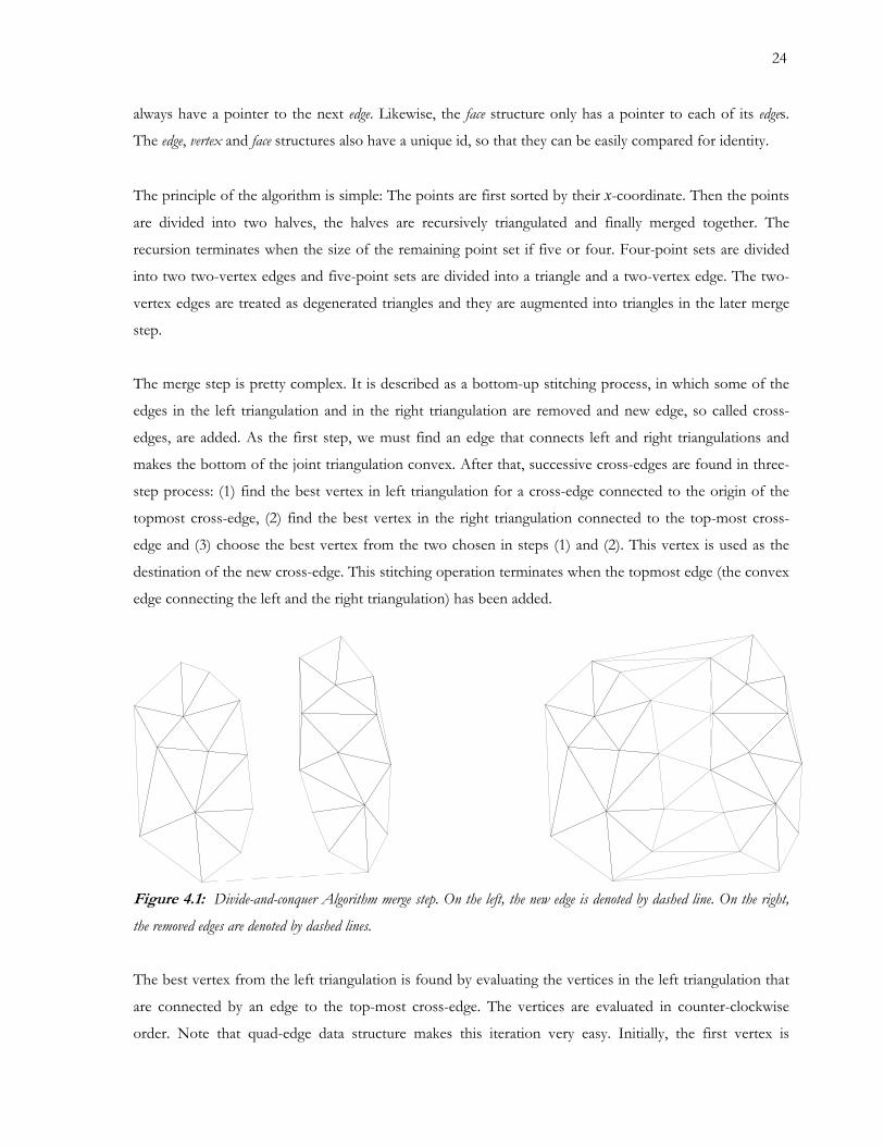
The merge step is pretty complex. It is described as a bottom-up stitching process, in w

e

makes the bottom of the joint triangula

s

topmost cross-edge, (2) find the best vertex in the right triangulation connected to the top-most cross-

edge and (3) choose the best vertex from the two chosen in steps (1) and (2). This vertex is used as the

destination of the new cross-edge. This stitching operation terminates when the topmost edge (the convex

edge connecting the left and the right triangulation) has been added.

Figure 4.1: Divide-and-conquer Algorithm merge step. On the left, the new edge is denoted by dashed line. On the right,

the removed edges are denoted by dashed lines.

The best vertex from the left triangulation is found by evaluating the vertices in the left triangulation that

are connected by an edge to the top-most cross-edge. The vertices are evaluated in counter-clockwise

order. Note that quad-edge data structure makes this iteration very easy. Initially, the first vertex is

25

assumed to be the best. The next vertex is better than it, if it is inside the circle defined by the current best

vertex and the two vertices of the top-most cross-edge. If the next vertex is better, the temporary edge is

.

Intuitively, divide-and-conquer algorithm proceeds sub-optimally, since the recursion divides the point set

into very long and narrow bands. Although these bands are triangulated so that they fulfil the Delaunay

criterion locally, they are pretty far from the final triangulation that globally fulfils the Delaunay criterion.

This short-coming in the algorithm has been noticed by many researchers and Rex Dwyer was the first to

suggest an enhancement to in [Dwye86] by using altering vertical and horizontal splits.

4.1.3 Radial Sweep Algorithm

The radial sweep algorithm is a straight-forward refining algorithm that is easy to implement. It first finds

a ithm then counts the

oint and sorts them by this angle and forms triangles between successive edges and in the non-convex

notches. This initial triangulation is then refined with the iterative edge-flip procedure. Radial sweep

algorithm was first described by Mirante and Weingarten in [MW82]. The initial triangulation produced by

the algorithm is very poor: it contains almost solely long, thin triangles.

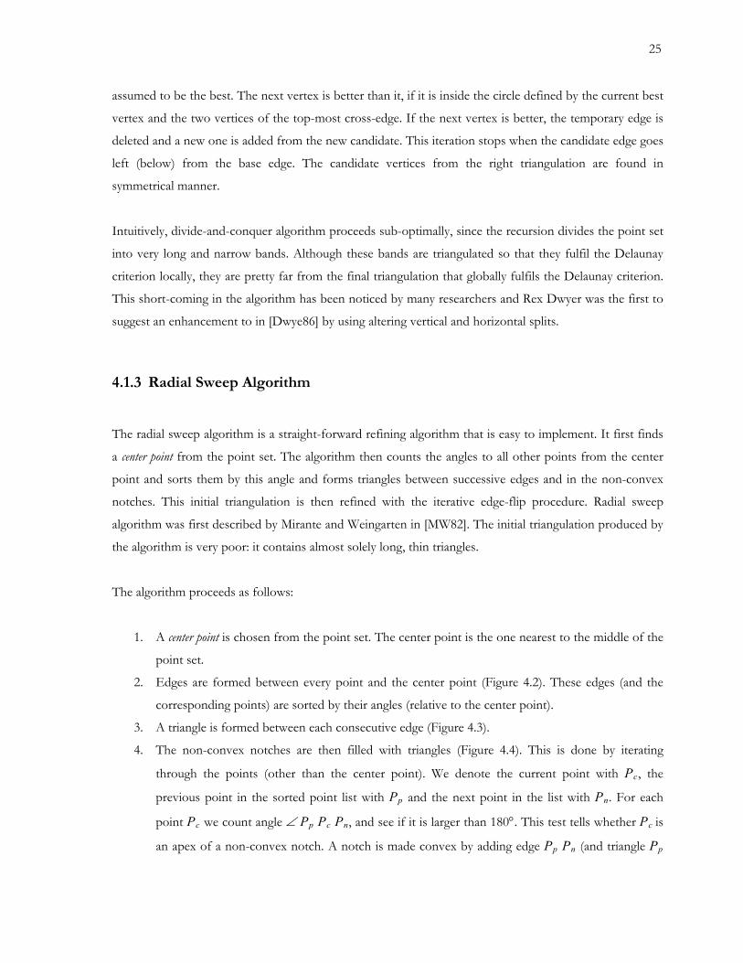
The algorithm proceeds as follows:

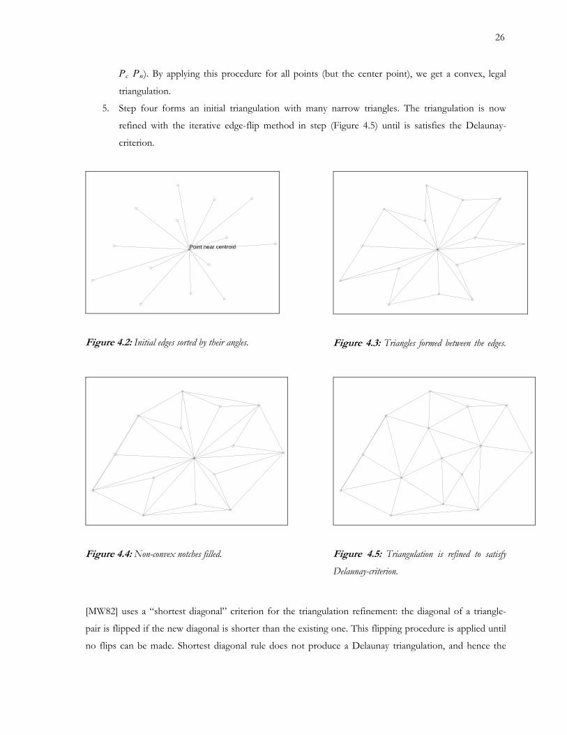
1. A center point is chosen from the point set. The center point is the one nearest to the middle of the

point set.

2. Edges are formed between every point and the center point (Figure 4.2). These edges (and the

corresponding points) are sorted by their angles (relati e to the center point).

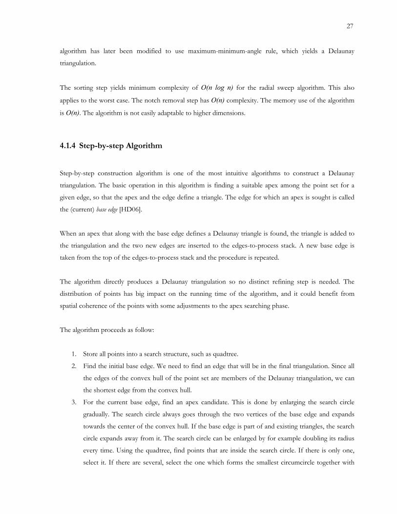
n each consecutive edge (Fi

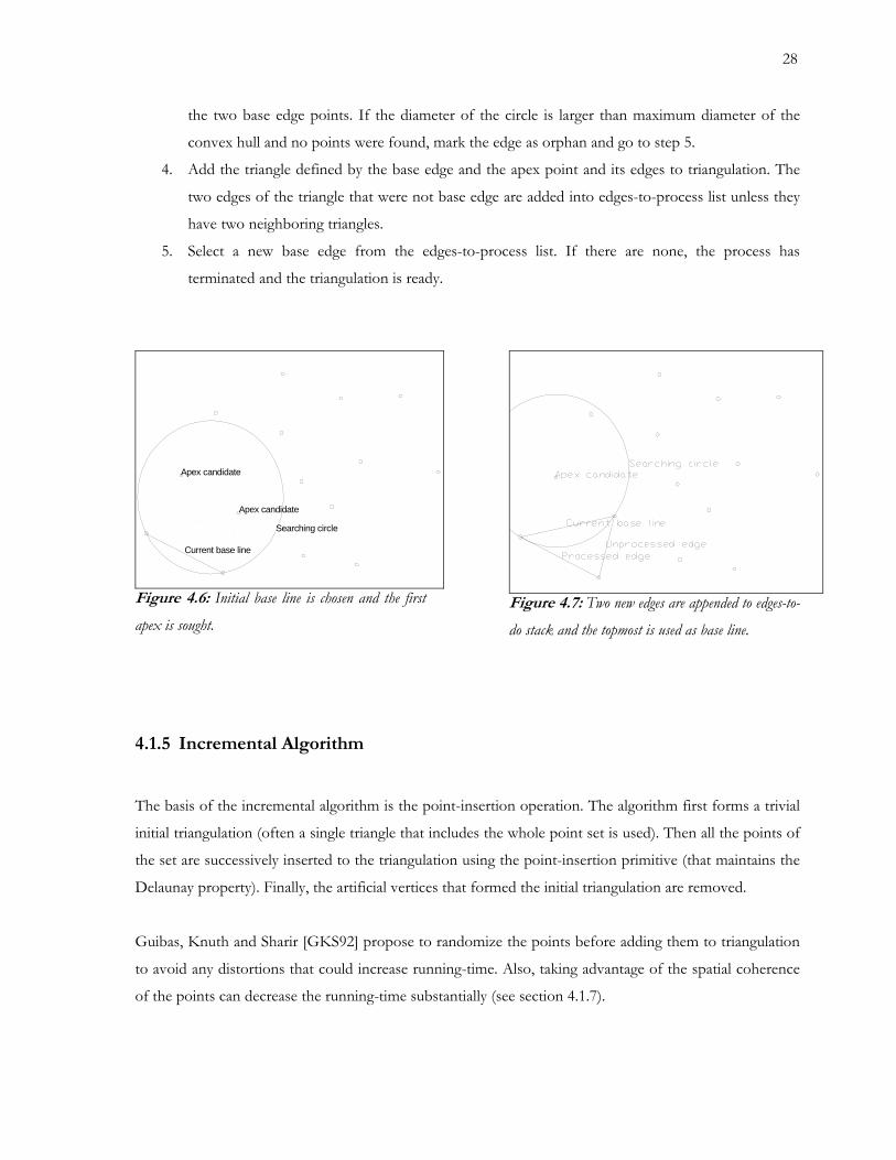
4. The non-convex notches are then filled with triang This is done by iterating

through the points (other than the center point). We denote the current point with Pc, the

deleted and a new one is added from the new candidate. This iteration stops when the candidate edge goes

left (below) from the base edge. The candidate vertices from the right triangulation are found in

symmetrical manner

center point from the point set. The algor angles to all other points from the center

p

v

3. A triangle is formed betwee gure 4.3).

les (Figure 4.4).

previous point in the sorted point list with Pp and the next point in the list with Pn. For each

point Pc we count angle ∠ Pp Pc Pn, and see if it is larger than 180°. This test tells whether Pc is

an apex of a non-convex notch. A notch is made convex by adding edge Pp Pn (and triangle Pp

26

lation.

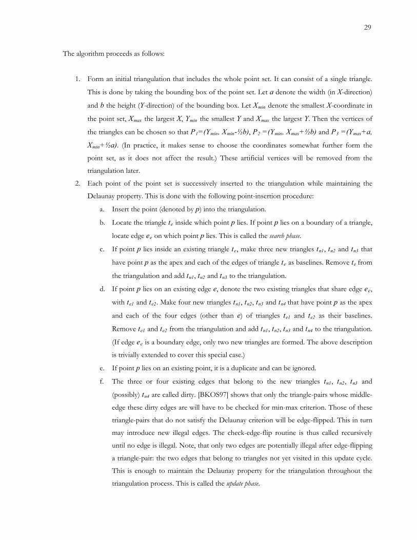
5. Step four forms an initial triangulation with many narrow triangles. The triangulation is now

Pc Pn). By applying this procedure for all points (but the center point), we get a convex, legal

triangu

refined with the iterative edge-flip method in step (Figure 4.5) until is satisfies the Delaunay-

criterion.

Point near centroid

Figure 4.2: Initial edges sorted by their angles.

Figure 4.3: Triangles formed between the edges.

Figure 4.4: Non-convex notches filled.

Figure 4.5: Triangulation is refined to satisfy

Delaunay-criterion.

[MW82] uses a “shortest diagonal” criterion for the triangulation refinement: the diagonal of a triangle-

pair is flipped if the new diagonal is shorter than the existing one. This flipping procedure is applied until

no flips can be made. Shortest diagonal rule does not produce a Delaunay triangulation, and hence the

27

algorithm has later been modified to use maximum-minimum-angle rule, which yields a Delaunay

triangulation.

The sorting step yields minimum complexity of O(n log n) for the radial sweep algorithm. This also

applies to the worst case. The notch removal step has O(n) complexity. The memory use of the algorithm

.1.4 Step-by-step Algorithm

Step-by-step construction algorithm is one of the most intuitive algorithms to construct a Delaunay

triangulation. The basic operation in this algorithm is finding a suitable apex among the point set for a

given edge, so that the apex and the edge define a triangle. The edge for which an apex is sought is called

the (current) base edge [HD06].

When an apex that along with the base edge defines a Delaunay triangle is found, the triangle is added to

the triangulation and the two new edges are inserted to the edges-to-process stack. A new base edge is

taken from the top of the edges-to-process stack and the procedure is repeated.

directly produces a Delaunay triangulation d. The

distribution of points has big impact on the running time of the algorithm, and it could benefit from

patial coherence of the points with some adjustments to the apex searching phase.

3. For the current base edge, find an apex candidate. This is done by enlarging the search circle

r example doubling its radius

every time. Using the quadtree, find points that are inside the search circle. If there is only one,

select it. If there are several, select the one which forms the smallest circumcircle together with

is O(n). The algorithm is not easily adaptable to higher dimensions.

4

The algorithm so no distinct refining step is neede

s

The algorithm proceeds as follow:

1. Store all points into a search structure, such as quadtree.

2. Find the initial base edge. We need to find an edge that will be in the final triangulation. Since all

the edges of the convex hull of the point set are members of the Delaunay triangulation, we can

the shortest edge from the convex hull.

gradually. The search circle always goes through the two vertices of the base edge and expands

towards the center of the convex hull. If the base edge is part of and existing triangles, the search

circle expands away from it. The search circle can be enlarged by fo

28

f the diameter of the circle is larger than maximum diameter of the

convex hull and no points were found, mark the edge as orphan and go to step 5.

the two base edge points. I

4. Add the triangle defined by the base edge and the apex point and its edges to triangulation. The

two edges of the triangle that were not base edge are added into edges-to-process list unless they

have two neighboring triangles.

5. Select a new base edge from the edges-to-process list. If there are none, the process has

terminated and the triangulation is ready.

Apex candidate

Current base line

Searching circle

Apex candidate

Figure 4.6:

apex is

Initial base line is chosen and the first Figure 4.7: Two nsought.

ew edges are appended to edges-to-

4.1.5

The basis of t

initial tria ation (often a single triangle that includes the whole point se the points of

the set are successively inse

Delaun

Guibas,

to avoid a

of the points can de

do stack and the topmost is used as base line.

Incremental Algorithm

he incremental algorithm is the point-insertion operation. The algorithm first forms a trivial

ngul t is used). Then all

rted to the triangulation using the point-insertion primitive (that maintains the

ay property). Finally, the artificial vertices that formed the initial triangulation are removed.

Knuth and Sharir [GKS92] propose to randomize the points before adding them to triangulation

ny distortions that could increase running-time. Also, taking advantage of the spatial coherence

crease the running-time substantially (see section 4.1.7).

29

The algorithm proceeds as follows:

1. Form an initial triangulation that includes the whole point set. It can consist of a single triangle.

This is done by taking the bounding box of the point set. Let a denote the width (in X-direction)

and b the height (Y-direction) of the bounding box. Let Xmin denote the smallest X-coordinate in

the point set, Xmax the largest X, Ymin the smallest Y and Xmax the largest Y. Then the vertices of

the triangles can be chosen so that P1=(Ymin, Xmin-½b), P2 =(Ymin, Xmax+½b) and P3 =(Ymax+a,

Xmin+½a). (In practice, it makes sense to choose the coordinates somewhat further form the

point set, as it does not affect the result.) These artificial vertices will be removed from the

triangulation later.

2. Each point of the point set is successively inserted to the triangulation while maintaining the

Delaunay property. This is done with the following point-insertion procedure:

a. Insert the point (denoted by p) into the triangulation.

b. Locate the triangle te inside which point p lies. If point p lies on a boundary of a triangle,

locate edge ee on which point p lies. This is called the search phase.

c. If point p lies inside an existing triangle te, make three new triangles tn1, tn2 and tn3 that

have point p as the apex and each of the e e te as baselines. Remove te from

the triangulation and add tn1, tn2 and tn3 to the triangulation.

ng edge e, denote e

with te1 and te2. Make four new triangles tn1 n2 n3 d tn4 that have point p as the apex

and each of the four edges (other than e) of triangles te1 and te2 as their baselines.

Remove te1 and te2 from the triangulation and add tn1, tn2, tn3 and tn4 to the triangulation.

(If edge ee is a boundary edge, only two new triangles are formed. The above description

is trivially extended to cover this special case.)

e. If point p lies on an existing point, it is a duplicate and can be ignored.

f. The three or four existing edges that belong to the new triangles tn1, tn2, tn3 and

(possibly) tn4 are called dirty. [BKOS97] shows that only the triangle-pairs whose middle-

edge these dirty edges are will have to be ecked for min-max criterion. Those of these

triangle-pairs that do not satisfy the Delaunay criterion will be edge-flipped. This in turn

s. The che

is illegal. Note, that only two egal after edge-flipping

a triangle-pair: the two edges that belong to triangles not yet visited in this update cycle.

This is enough to maintain the Delaunay property for the triangulation throughout the

triangulation process. This is called the update phase.

dges of triangl

d. If point p lies on an existi the two existing triangles that share edge e ,

, t , t an

ch

may introduce new illegal edge

until no edge

ck-edge-flip routine is thus called recursively

edges are potentially ill

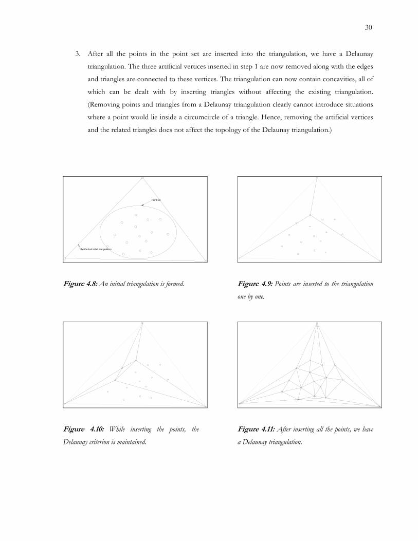
30

3. After all the points in the point set are inserted into the triangulation, we have a Delaunay

triangulation. The three artificial vertices inserted in step 1 are now removed along with the edges

and triangles are connected to these vertices. The triangulation can now contain concavities, all of

which can be dealt with by inserting triangles without affecting the existing triangulation.

(Removing points and triangles from a Delaunay triangulation clearly cannot introduce situations

where a point would lie inside a circumcircle of a triangle. Hence, removing the artificial vertices

and the related triangles does not affect the topology of the Delaunay triangulation.)

Point set

Synthetical initial triangulation

Figure 4.8: An initial triangulation is formed.

lation

Figure 4.9: Points are inserted to the triangu

one by one.

Figure 4.10:

Delaunay criterion is mai

Figure 4.11: After inserting all the points, w

a Delaunay triangulation.

While inserting the points, the

ntained.

e have

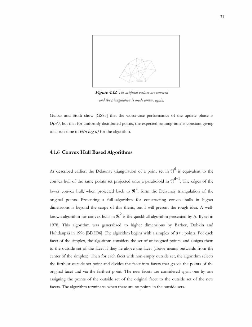
31

Figure 4.12: The artificial vertices are removed

and the triangulation is made convex again.

and Stolfi show [GS85] that the worst-case performance of the update phase is 2

own algorithm for convex hulls in ℜ2 is the quickhull algorithm presented by A. Bykat in

1978. This algorithm was generalized to higher dimensions by Barber, Dobkin and

lex of d+1 points. For each

cet of the simplex, the algorithm considers the set of unassigned points, and assigns them

facets. The algorithm terminates when there are no points in the outside sets.

Guibas

O(n ), but that for uniformly distributed points, the expected running-time is constant giving

total run-time of Θ(n log n) for the algorithm.

4.1.6 Convex Hull Based Algorithms

As described earlier, the Delaunay triangulation of a point set in ℜd is equivalent to the

convex hull of the same points set projected onto a paraboloid in ℜd+1. The edges of the

lower convex hull, when projected back to ℜd, form the Delaunay triangulation of the

original points. Presenting a full algorithm for constructing convex hulls in higher

dimensions is beyond the scope of this thesis, but I will present the rough idea. A well-

kn

Huhdanpää in 1996 [BDH96]. The algorithm begins with a simp

fa

to the outside set of the facet if they lie above the facet (above means outwards from the

center of the simplex). Then for each facet with non-empty outside set, the algorithm selects

the furthest outside set point and divides the facet into facets that go via the points of the

original facet and via the farthest point. The new facets are considered again one by one

assigning the points of the outside set of the original facet to the outside set of the new

32

To generate the Delaunay triangulation of a point set in ℜ2, the points are first projected

nto a 3D paraboloid

.1.7 Specialized Cases

the partitions by removing the already processed areas from the active set and

cusing on a small are at a time. They describe the speed up as stunning: they were able to

a that has sufficient spatial coherency, but they claim that a large part

f real world data has.

nly points. Rather, obvious fold-lines, such

the base line of a drain, the side of a road or the wall-line of a building, can be included in

iangulation. Therefore, no

o

z = x2 +y2

In this case, the 3D convex hull consists of triangles. The triangles are projected back to ℜ2

ignoring the ones whose normal doesn’t point outwards from the paraboloid. The result is

the Delaunay triangulation of the original point set.

4

In some cases it is worthwhile to take advantage of the known properties of the input data.

Isenburg et al [ILSS06] describe a streaming algorithm to compute the Delaunay

triangulation of a huge, well-distributed points set. The algorithm exploits the natural spatial

coherence in a stream of points that is often present in real world data because of the way

the surveying equipment operates. The algorithm is based on incremental algorithm

described in section 4.1.5. The point data is first partitioned and tagged with finalization tags

that indicate the point is the first in that region. The incremental algorithm can then take

advantage of

fo

process 11.2 GB of water radar point data in 48 minutes using only 70 MB of memory. This

is only possible for dat

o

4.2 Point Data Triangulation with Fold-lines

The measured data usually does not consist of o

as

the data. The fold-lines are polylines. They consist of points and edges that connect the

points. The points of the fold-lines will appear as vertices in the final triangulation. The fold-

lines define a fold that must appear in the geometry of the final tr

33

triangle in the final triangulation can cross the fold-line, only touch it. It is easy to see that

the edges of the fold-lines therefore also appear as edges in the final triangulation.

ue to this, I have chosen the approach of treating the fold-line edges as pre-defined and

e Delaunay criterion, it is necessary to find a secondary criterion

r triangle “goodness”. The min-max criterion used in the point-data triangulation turns out

to be good for this. It has been proven that iteratively applying min-max –based edge-swap

a Delaunay TIN. Even if the TIN cannot satisfy the

elaunay criterion, applying min-max yields a good TIN that is as close to the Delaunay TIN

wap

than before the swap, swap.

3. If the number of triangles that satisfy the Delaunay criterion is equal after and

before the swap, use min-max criterion.

Since fold-lines are an additional constraint to the algorithm, they tend to increase running-

time. It is, however, possible to try to exploit these constraints in some cases to avoid

unnecessary searches on areas where no edge swaps can be made.

D

fixed edges in the triangulation process. This approach works well if the basic point-data

triangulation algorithm is based on searching new triangles edge by edge. The only strictly

needed modification to the algorithm is preventing the edge-swap function from touching

“fixed” edges. The algorithm already has to find out whether the new edge candidates cross

with existing edges (fixed or not), thus this introduces no problem.

Because fold-lines can introduce arbitrary constraints to the triangulation, the resulting

triangulation rarely fulfils the Delaunay criterion. It is therefore difficult to unambiguously

define the criteria for a fold-line-constrained triangulation. Obviously, fixed edges (fold-lines)

are a mandatory criterion. But because fold-lines mandate only few edge-swap decisions, and

all triangles cannot satisfy th

fo

to an arbitrary TIN eventually yields

D

as possible.

My algorithm obeys the following rules when deciding whether to perform an edge-swap for

a triangle-pair:

1. If the triangle-pair’s middle-edge is fixed, do not swap

2. If the number of triangles that satisfy the Delaunay criterion is larger after the s

34

4.2.1 Other Approaches

most commonly used approach is to triangulate the point-data

ncluding the vertices from the fold-lines) like before. Then, a separate algorithm that takes

algorithm. It is possible to take a known-to-be-robust point data

iangulation algorithm, and implement the fold-line support to it as a mere post-processing

Other approaches exist. The

(i

the fold-lines and the point-data triangulation as input edge-swaps the triangle-pairs whose

middle edge crosses the fold-line. (The triangulation in the neighborhood of the edge-swap

can then be refined to be as close to Delaunay triangulation as possible).

The reason this approach is so popular is that it requires no changes whatsoever to the point

data triangulation

tr

procedure. It does seem more optimal to take the fold-lines in consideration during the point

data triangulation because

4.2.2 Additional Constraints

Often, additional fold-line related constraints are imposed to the triangulation. Most

common of these is that a triangle in the final triangulation may not have two edges on the

same fold-line. This is because the fold-lines are often altitude contours on an even altitude.

If a triangle has two lines on a contour, it is obviously has the same Z for all points. This

makes it impossible to unambiguously resolve the height line for that altitude from the

resulting triangulation. Implementing this requirement to the triangulation algorithm is

straightforward: rule out such triangles during the apex searching and edge-swap phase.

35

5 Manipulating and Using an Existing Triangulation

so that the resulting triangulation satisfies the

elaunay criterion, one can use the incremental algorithm steps 2 and 3 described in section

n, we first find the first vertex on the boundary of the existing

iangulation from which we can add an edge to the new point without crossing any existing

edges. For this, it is enough the check the edges of the triangles connected to the candidate

found, we add an edge between it and the new point to the

iangulation. We then continue iterating the vertices on the boundary clockwise adding

that the incremental method is among the two fastest ones.

5.1 Adding a Point

To add a point to a Delaunay triangulation

D

4.1.5. As discussed in section 4.1.5, it is enough to check the neighboring triangle-pairs for

Delaunay criterion and possibly edge-flip them, and their neighbors recursively. While the

worst case complexity of this is linear, the amortized complexity is constant for uniformly

distributed points.

If the point lies on an existing triangle vertex, it can be ignored. If the point lies outside the

boundary of the existing triangulation, a procedure somewhat dissimilar to the incremental

algorithm point addition must be used. (Recall that in the incremental algorithm, it was first

made sure that the initial triangle surrounds all the points to be triangulated.) In this case,

searching clockwise-directio

tr

vertex. After this first vertex is

tr

edges to triangulation until adding an edge would cross an existing edge. We add a triangle

between each successive new edge. After this, we must check each triangle-pair whose other

triangle is a new triangle for Delaunay criterion and potentially edge-flip it. In this case, the

complexity of point addition is O(k), where k is the number of vertices on the boundary of

the triangulation. For pathological cases, this can be as much as O(n), where n is the number

of points in the triangulation (if all the points are on a convex, arc like curve.) In practice,

this is never the case.

In addition to the incremental method described above, there are other methods to update a

Delaunay triangulation. Guibas and Russel [GR04] compare four different methods, and find

36

5.2 Adding a Set of Points

imply by iterating the procedure for

dding a single point described in section 5.1. The amortized complexity of this is O(k),

e e k is the number of points to be added.

owever, certain special cases, optimizations can be made. If, for example, it is known that a

described in section 4.1.4. Unless the line is vertical,

e merge step must be modified so that it evaluated its criteria relative to the line and not

.3 Deleting a Point

cts the neighborhood of the removed

oint. We first remove the point, and the edges adjacent to it. We now have an empty

triangulate.

A set of points can be inserted with reasonable cost s

a

wh r

H

large number of points lies outside the existing triangulation, and they are located so that a

straight line can be drawn between them and the existing triangulation, the set of new points

can be triangulated separately and then merged to the existing triangulation using the merge

step of divide-and-conquer algorithm

th

vertically. This is clearly non-trivial, and probably not worth the trouble in general case, but

in special cases it could reduce the complexity of adding a set of points from O(n·k), where n

is the number of triangles in the existing triangulation and k is the number of points to be

added, to O(k log k + n).

5

Similarly to adding a point, removing one only affe

p

polygon in the middle of the triangulation. (Unless the removed point was a vertex of a

boundary triangle – if so, we leave the edge of that belonged to the boundary of the

triangulation in place.) We triangulate this polygon and add the new triangles into the

triangulation. Note that removing a point and its adjacent triangles from a Delaunay

triangulation always yields a convex hole. Thus, the hole is very easy to

The triangulation now doesn’t fulfill the Delaunay criterion. We can now use the incremental

algorithm update phase process described in section 4.1.5 with slight modifications: we call

37

the check-and-flip routine for all the new edges and the edges that are part of the boundary

.4 Deleting a Set of Points

e can just call the single point removal

utine outlined in section 5.3 repeatedly. The incremental algorithm update phase can be

angles, we update it to fulfill the Delaunay criterion as in

ction 5.3.

of the hole, and recursively for all the affected edges.

The worst case complexity of this is from O(n), where n is the number of triangles in the

existing triangulation, but amortized, it turns constant.

5

If the points are scattered all over the triangulation, w

ro

postponed to after all points have been added. This way, some edges do not need to be

checked and swapped multiple times.

If we are to remove a large number of neighboring points (connected with one edge), we can

first remove all of them and their adjacent triangles. This creates a potentially non-convex

hole. This hole can again be triangulated as in section 5.3. Although triangulating non-convex

is not as trivial as triangulating convex ones, there are many good algorithms for that. After

the hole has been filled with new tri

se

5.5 Folding with a Line or a Polyline

We often know certain vertices are connected by edges to form a ridge or ditch. This often

the case for road plans or other built areas. Such ridge or ditch is called a fold-line because it

folds the surface. A fold-line can consist of one or more line segments, i.e. it can be a

polyline. Each line segment of the fold-line is a constrained edge in the triangulation: it

cannot be edge-flipped even if it violates the Delaunay triangulation.

To add a new fold-line to an existing triangulation we must first make sure all its vertices are

present in the triangulation. We add them into the triangulation with the incremental

algorithm point adding method as described in section 5.2.

38

The next step is to make sure the new constrained edges are present in the triangulation. For

each fold-line edge, we identify the triangles that lie between the vertices of the edge, remove

them, add the new edge, and fill the hole to left and right of the new edge with triangles. We

can apply the incremental algorithm update phase to the new edges (see section 4.1.5), but

we cannot flip the new constrained edge. Hence, the triangulation will potentially not satisfy

e Delaunay criterion anymore.

angulation must

ive as similar results as the original triangulation as possible. I.e. it must maintain the z

te at any given point as well as possible. If the triangulation is used for visualization,

original triangulation from the

iven viewing distances and angles.

llapsed: the triangles

eighboring it are removed, and a new vertex is added in the middle of the removed edge.

Each edge collapse reduces the triangulation with one point, two triangles and three edges.

th

5.6 Simplifying the Triangulation

Simplification or reduction of the triangulation is a process where the complexity of the

triangulation is reduced trying to maintain the properties of the triangulation as well as

possible. The properties that need to be maintained depend on the application. If the

triangulation is used for interpolation and volume calculation, the reduced tri

g

coordina

the reduced triangulation must look similar enough to the

g

The purpose of the simplification is to save memory (both long-term and short-term) and

processing time when using the triangulation. The triangulation might consist of millions of

vertices, large majority of which are redundant for the given application.

There are different methods to simplify a triangulation. One can for example interpolate

points on the triangulation at desired interval and then re-triangulate the new point set. This

is usually too complex. A common approach is so called edge-collapse algorithm. In this

algorithm, the edges of the triangulation are evaluated one at a time. For each edge, it is

checked if it satisfies the collapse criterion (which can be fine-tuned, but usually takes the 2D

length of the edge and the height difference of the edge in consideration and value them with

certain weights.) If the edge is considered unimportant enough, it is co

n

39

Depending on the application, we may want to simplify the triangulation to certain amount

of vertices (e.g. visualization with constant frame rate) or so that it still meets a quality

criterion (interpolation). Straight-forward edge-collapse algorithm gives the latter, but it may

be extended to give the former by iteratively applying the simplification several times relaxing

e quality criteria each time until the triangulation has less than wanted amount of points.

ally Refining the Triangulation

th

One interesting development of triangulation simplification is a concept called progressive

meshes [Hop96]. Much like progressive bitmap image formats (such as progressive JPEG),

they can be used to transmit the mesh over network so that the receiving end can first

present a rough shape of the mesh and it is then refined as the transmission proceeds. They

can also be used to render large meshes with dynamic level of detail: higher detail near the

camera and rougher representation further away. There are several methods to implement

progressive meshes, but the initial idea by Hoppe was based on encoding the edge collapses

and then applying them backwards when progressively enhancing the mesh.

5.7 Artifici

A Delaunay triangulation that is contains the given input vertices (and edges) and nothing

more may not be satisfactory to all purposes. While MWT is theoretically optimal, some

argue that a Delaunay triangulation of a given point set is the optimal triangulation for

interpolating heights. A Delaunay triangulation is good for many other purposes as well. It is

worth noting, however, that if the input includes predefined edges, the resulting triangulation

does not always fulfill the Delaunay criterion. The result might not be unambiguous either.

Since there is only one possible Delaunay triangulation for a given point set (provided that it

is in general position) it is not possible to enhance the triangulation without either breaking

the Delaunay property or adding points. Breaking the Delaunay criterion is clearly not

desirable. Altering a constrained triangulation (a contrivance we might get away without

adding more non-Delaunay triangles) is not likely to give too good results either, since the

triangulation is already produced using a metric to maximize its quality.

40

Despite being a Delaunay one, the triangulation at hand might still be unsatisfactory. It can

contain long, narrow triangles (in particular, near its borders) that have very narrow angles.

Another quality that is not always acceptable is the variance in the sizes of the triangles; the

iangulation might contain very large and very small triangles. In many cases, homogeneity

we can get rid of the narrow and large triangles. [Rup95] discusses one of the

rst good algorithms to do this. Ruppert’s algorithm is guaranteed to yield a triangulation

that satisfied the given bound for minimum angle while using relatively few triangles.

elaunay triangulation of

e input point set. At the second stage, it alters the triangulation so that it satisfies the fold-

ight contain a hole or a concavity where there is a lake or a spot where there is no

easured data.

ses in which the algorithm adds a

ertex. First, if the diametrical circle of an edge (smallest circle that contains the edge)

condition (no other points on the circumcircle of an edge) has been dealt with, the second

one will always add the vertex inside the triangle at hand because the triangle satisfies the

Delaunay criterion. [Rup95] also discusses why this will always make the angles larger and

7˚ (with most inputs it

nates even with angle constraint of 33.8˚.)

tr

in this respect is desired.

What can we do to enhance the triangulation? One possibility is to intelligently add more

vertices so that

fi

Ruppert’s algorithm proceeds in four stages. First, it produces a D

th

line constraints. The result of these two steps is a constrained Delaunay triangulation–

producing such triangulation is discussed in depth in Chapters 5 and 6, so I’ll omit the

Ruppert’s approach here. The third stage of the algorithm removes concavities and holes in

the triangulation. This is because desired triangulation is not always convex; for example, a

surface m

m

The fourth step of the Ruppert’s algorithm is what is truly interesting. The algorithm adds

vertices to the triangulation preserving the Delaunay criterion using a variant of the point

addition algorithm discussed in 7.1. There are two ca

v

contains a point other that the two ends of the edge, a vertex is added in the middle of the

edge. The two halves of the edge are then recursively checked for the same criterion and

divided if necessary. Second, if a triangle has an angle that is smaller than the desired value,

the triangle is divided by inserting a vertex in the center of its circumcircle. After the first

proves that his algorithm halts for an angle constraint of up to 20.

termi

41

In 2.5-dimensional and triangulations, the height of the added vertex is simply interpolated

from the edge or from the triangle using the algorithm described in section 5.8. This ensures

the area and volume of the triangulation doesn’t change during the division.

Although Ruppert does not discuss it, the algorithm could easily be modified to also divide

too large triangles simply by triggering triangle division for example with an area criterion:

the 2D area of the triangle is calculated and the triangle is divided, if the area is smaller than

the threshold.

5.8 Interpolating a Height Value for a 2D Point

In infrastructure design applications this is the most fundamental operation to be performed

using a digital terrain model. Each time we add an object such as lamp post, traffic sign, or a

corner of a building into the 3D construction plan, we must know where on the surface it

lies. The x and y coordinates are given, but z must be interpolated from the digital terrain

model.

For a triangulation, this operation is simple. First, locate the triangle the point lies in. If it lies

on an edge, we can use either triangle. If it lies on a vertex, we can just return the height of

that vertex, or use any of the triangles connected to that vertex to avoid special casing. Then,

interpolate the height of the point from the triangle.

Interpolating a height of a point from a triangle is easy. Let us consider a vertex of the

triangle to be the origin. Vectors v2 and v3 point from the origin vertex to the two other

vertices and vector p points from the origin to the goal point. Let vector c to be the cross

product of vectors v2 and v3. The height of the goal point relative to the origin vertex then is

z

yyxx

cpcpc

z−

+=

For final result, we add the z of the origin vertex to that [HW99].

Unless we keep some kind of lookup index or have the triangles ordered somehow, locating

the triangle has linear complexity, which is not acceptable. We can order the triangles by the

42

x coordinate or their leftmost vertex and record the width of the widest triangle (triangle

o e leftmost vertex is furthest away from the rightmost vertex in x direction.) Then, we

ftmost vertex is left of the interpolated

oint. We can then iterate triangles leftward until we find a triangle that contains the goal

ery wide, perhaps as wide as the

hole triangulation. This would turn this approach into O(n) complexity. However, in

lthough sorting the triangles by their x coordinate is free with regards to memory usage, it

wh s

can use binary search to find the first triangle whose le

p

point. We can also terminate the iteration when we are further away (in x direction) from the

goal point than the width of the widest triangle. If we haven’t found the triangle that includes

the goal point by then, it cannot exist in the triangulation. For an arbitrary triangulation,

there is no guarantee that the widest triangle would not be v

w

Delaunay triangulation, the triangles are very well formed, so this cannot happen but for the

most pathological cases.

If we choose to maintain the neighborhood information for each triangle in our final data

structures (which triangle is neighbor of which triangle), we can enhance the algorithm

somewhat. First we locate the initial triangle that is close to the goal point. We then draw a

line from the center of that triangle to the goal point, and see which of the three edges of the

triangle it intersects. We then move to the triangle that shares that edge with the current

triangle. We then draw a new line from the center of the current triangle and repeat this

process until we have found the triangle the goal point lies in (i.e. the line does not intersect

any of the edge of the triangle.) This has the same worst case complexity, but is faster in

practice. Maintaining the neighborhood information introduces a memory cost of 3 indices

per triangle.

A

is suboptimal for searching the closest triangles. This is why many practical applications

choose to maintain an auxiliary spatial index of the points. Most common type of index is

the quadtree structure. A quadtree recursively subdivides an area into four segments: lower

left, lower right, upper left and upper right [Knu98]. Each segment has its own sub-tree and

is again divided in four sections until each segment contains less than certain amount of

items. Such segment is a leaf of a tree and contains a list of elements that belong to it. For

every segment (leaf or not), we know that the sub-tree pointed by it contains all the elements

that lie on the area of the segment [BKOS97]. Although searching a quadtree takes

logarithmic time, it is much faster than binary searching sorted triangles in practice.

43

5.9 Interpolating a Line or a Polyline

Another very common operation for digital terrain models in infrastructure design

a polyline onto the surface. Suppose for example that

e are to build a house or a fence on the ground. We know the 2D polyline that defines the

ribed

section 5.8. First we find the origin triangle as when interpolating a point, using the start

We also record the points where the line has

tersected the edge of triangles. (The 2D location of those points will be the 2D intersection

ent is the last, we also interpolate the

st point and append that. The recorded point chain is now the interpolated polyline.

by defining the intersection so that a line does intersect an edge if it touches the start point,

application is interpolating a line or

w

wall, but we also need to know where it lies on the ground.

For a triangulation, the procedure is as follows. For every line segment of the polyline, locate

every triangle in the triangulation the line segment touches. Provided we have the

neighborhood information available, we can use the neighboring triangle method desc

in

point of the line segment as the goal point. After this, we use the end point of the line

segment as the goal point and use the line segment we have at all time, and do not draw a

new line from the center of the current triangle.

in

point of the edge and the line, and the z is the z of the edge at that point.) For the next line

segment, we can omit the initial origin triangle search, since the end point of the previous

line segment is the start point of the next. After interpolating the intersection points of a line

segment, we interpolate the height of the start point of the line segment and prepend that

point in the list of intersection points. If the line segm

la

Unless we have the neighborhood information available, we need to search the triangles the

line segment touches from a quadtree (or similar), and then intersect them with the line.

Intersecting a triangle with a line in 2D gives two points if the triangle and the line intersect.

For degenerated triangles, it can also give three, and if the line and the triangle touch at one

point, it can give one. The former case can be ignored, because there should not be

degenerate triangles in Delaunay triangulations. The latter case can be ignored, because it

would not contribute any length to the polyline. It can also give three points, if the line

comes into the triangle at a vertex and leaves through an edge. We can subvert this problem

44

but not end point. We form a line segment between these two points. Once we have

intersected all the triangles the quadtree search gave us, we have a list of line segments that

e will stitch together if they share a vertex.

tely as possible. When the

olumes are known, different design alternatives can be compared based on their cost.

two surfaces.

Both of these cases are relatively straight-forward if we are only interested in the absolute

re design applications, we must

often known how much of the surface is above (or under) the comparison plane (or surface)

eas. These are called the

xcavation and fill areas. We will come into that later.

w

5.10 Calculating Volume

In infrastructure construction, moving, removing and adding large quantities of soil material

is a laborious and expensive operation. Suitable gravel must be brought in from a stone-pit

far away, and even the waste soil can’t be dumped wherever in urban environment. This is

why the volumes of the soil materials must be know as accura

v

There are two cases how volume is calculated from a digital terrain model. The simple case is

when the volume is calculated against a given height (plane). The more complex case is when

the volume is calculated between

volume between the two surfaces. However, in infrastructu

and give the 2D area, volume and bounding polylines of those ar

e

The volume is usually calculated on a given 2D area, bounded by a given polyline. The first

step is then to divide the surface with the bounding polyline. We first fold the triangulation

with the boundary line as described in section 5.5. We then remove (or ignore) all the

triangles outside the boundary line. If we are calculating the volume between two

triangulations, we do this for the other triangulation, too. We now have two triangulations

whose 2D area and projection are identical. We then calculate the volume between z=0 and

the triangle (or z of the comparison plane). This volume is the 2D area of the triangle

multiplied with the average of the heights of the vertices of the triangle (or height compared

to the comparison plane). We take the sum of all these volumes to get the final absolute

45

volume. If we are comparing to a triangulation, and not to a plane, we calculate its absolute

volume in similar manner and decrement it from the volume we calculated earlier.

r manner. For each triangle we must see inside

hich fill or excavation boundary polyline it lies and add its volume to the fill volume or

.1 Robustness of the Triangulation Algorithm

If we must know the excavation and fill areas, we must first find the places where the

surfaces (or surface and a plane) intersect. In case of plane, this is easy: first locate all the

triangles in the triangulation that have (at least) one vertex below the plane and one above.

Then calculate the line where the triangle intersects the plane. Then stitch a polyline out of

these line segments. The polyline will either be closed or connected to the boundary polyline,

in which case we can make it closed via the boundary line. We then fold the triangulation

with these polylines and calculate the volume of each triangle. Positive volumes add to the

fill volume and negative volumes add to the excavation volume.

For surface against surface calculation, we must fold both surfaces and calculate the volumes

of the triangles of the both surfaces in simila

w

excavation volume accordingly.

6 Implementation Considerations

6

As for example Guibas and Stolfi [Gui96] note, geometric data usually consists of both

numerical coordinates (numerical data) and combinatorial data. For example, a polytope data

structure contains a set of points whose coordinates are expressed with numbers (floating

point, integer, rational) and whose connectivity is expressed with the order of the points.

Obviously, the connectivity is unambiguous. But computing whether the polytope is convex

is not. A small inaccuracy during the execution of the algorithm (such as rounding a floating

point number) could disturb the algorithm if three points are nearly collinear. Even if exact

arithmetic was used, the problem remains. Many intermediate results such as distances

(which involve taking square root) cannot be expressed in rational numbers. Furthermore,

even algorithms that can completely be calculated used rational numbers tend to suffer from

46

intolerable memory and CPU time requirements as the each calculation can add to the bit

onstructions produce the output of

e algorithm. The predicates need to be exact, but the constructions will require the

ult.

aunay triangulation algorithms. He uses

approximat oduce error ε into the results and

shows that t is topologically correct

numbers

ontain an exponent and mantissa parts as well as a sign bit. The exponent part expresses the

agnitude of the number whereas the mantissa expresses the meaningful digits. This makes

e location of the decimal point meaningless to the precision of the calculation. However, in

the real world geometrical calculations, the locations are often expressed in global or

ile the actual data site is relatively small. Because every location

ncodes both the global location and site-local position, several meaningful digits of

the result contains coordinates.)

complexity of the rational numbers [For96].

Numerical precision, degenerate data sets or intermediate results, and other robustness issues

continue to be the most challenging problem in implementing geometrical algorithms. Over

the years, several strategies have been suggested to overcome the problems. Franco P.

Preparata [Pre96] suggests dividing the operations in the algorithm in two categories:

predicates and constructions. These operations have distinct role in the algorithm: predicates

determine the branching flow of the program whereas c

th

precision that ultimately produces the output precision required by the application. The

required numerical output precision can very greatly – in raster graphics, for example, the

requirement is pretty low – but is the predicates produce wrong results, the whole algorithm

can produce (topologically) incorrect res

Fortune [For92] studies the robustness of Del

e arithmetic, where operations +, -, × and ÷ intr

some algorithms can be implemented so that the resul

even with such arithmetic. In particular, incremental algorithm (see section 4.1.5) can be

implemented reliably in that case.

The IEEE 754 floating point numbers [VB04] are the de facto standard in modern computer

programming. They are engineered to produce good results with limited precision (32 or 64

bit), while being very fast to implement in hardware. The IEEE 754 floating point

c

m

th

country-wide coordinates, wh

e

precision are wasted. A common way to overcome this problem is to first find the center of

the data set, then translate it near to the origin, calculate, and then translate the result back (if

47

An algorithm that calculates a triangulation takes both numerical and combinatorial input,

ut only gives combinatorial output. In addition, most Delaunay triangulation algorithms

e modified to use any kind of number representation.

edges do not cross each other

riangulation given the same input (in

whatever precision – the term “same” here means that the bit-representation of the

)

the algorithm produces the same triangulation even if the point set is rotated on the

XY plane (except when there are points whose distance from a Delaunay disc is

raditionally in infrastructure design software, the triangulations are presented as an array of

b

need to calculate distances; so using exact arithmetic is not a good solution. In reality it is not

feasible to use anything but floating point numbers with data sets as large as hundreds of

thousands of points. Even in future, when the available computing power and memory

capacity will be larger, it is likely that the extra power will be used to tackle larger data sets.

This, however, is ultimately a preference question, and the algorithm (if designed wisely) can

b

With real world data sets, there is measuring error whose upper limit is not even always

known. This will makes impossible to guarantee a robust triangulation–a small error in the

data might cause the triangulation to be different from the right (Delaunay) one. What it is

possible to guarantee, however, is that

• The triangulation is topologically correct:

triangles are not inside each other (in 2D)

• the algorithm always produces the same t

coordinates is the same

•

smaller than the error that the rotation and related rounding can introduce)

6.2 Data Structures

T

points and array of triangles that contain three indices to the points array. For triangulating,

48

this data structure must usually be augmented with the neighboring triangles indices, three

for each triangle, to represent the topology needed in the triangulation process.

Guibas and Stolfi [Gui96] propose the Quad-Edge data structure to implement the divide-

and-conquer algorithm (see 5.1.2). In it, the edge is the central object, and it always contains

nks to the two neighboring triangles. See 5.1.2 for more detailed description of this data

ructures. His findings are interesting. Despite the quad-edge based code being more simple

and elegant, the triangle array (augmented with neighbor information) was generally as much

addition to the triangle array data

ructure: he added so-called ghost triangles where the triangles had no neighbors. These

With the multi-core processors becoming more and more common, parallel execution of

heavy calculations is more and more important.

Most of the Delaunay triangulation algorithms are not easily parallelizable – because they

modify the data structures at unlimited locations one would need to use very fine-grained

locking to safely parallelize them. This would probably negate any performance gain available

from parallel execution.

However, the divide-and-conquer algorithm (5.1.2) keeps the modifications localized. After

each divide step, both point subsets can be triangulated in separate thread and then merged

li

structure. It has the advantage that all the operations such as finding the neighboring edges

and triangles are fast. It also consumes more memory than the triangle array data structure.

Shewchuk [She96] has implemented several Delaunay triangulation algorithms with both data

st

as two times faster. Shewchuk made an innovative

st

ghost triangles lack one vertex (a null pointer) and link to each other as neighbors in addition

of the real boundary triangle. This got rid of several special case handling routines.

Like in so many algorithm design and implementation cases, the selection of – and even

invention of – data structures plays crucial role here.

6.3 Multi-threading

49

together. The two threads can’t add triangles into the same data structure, but to two

separate data structures which are then merged into one much like in merge sort. The

ch new point subset until

desired number of threads (e.g. one thread per processor core) has been launched. After that,

nquer algorithm, there has been research on parallelizing other

gorithms. [KK03] describes how incremental algorithm can be made parallel. Jonathan C.

s

apters, and non-general purpose processing units like the IBM Cell processing units

rocessing units (GPUs) for general purpose work is called

GP ower, but they can’t be programmed

th a t al [RTCS08] have

plem GPGPU.

recursion can be modified so that a new thread is launched for ea

the algorithm can proceed normally.

In addition to divide-and-co

al

Hardwick [Har97] describes an algorithm parallelizable over a cluster of workstations that

uses an efficient subdivision method and fine-tuned serial algorithm for the recursion leaves.

6.4 Non-General Purpose Processors

In addition to multi-threading, a rising trend of computing in the few past years have been

using non-general purpose processing units for general purpose work. And example of such

processing units would be the graphics processing units found in the modern graphic

ad

[Bar07]. Using the graphics p

GP U. These units have tremendous processing p

wi general purpose programming language. Guodong Rong a

im e to produce a Delaunay triangulation withnted algorithm

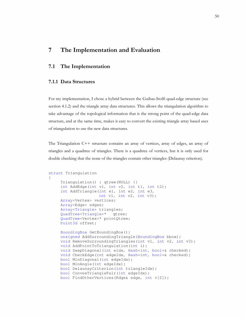
50

7 The Implementation and Evaluation

7.1 The Implementation

m structure (see

on ation algorithm to

ntage of the topological information that is the strong point of the quad-edge data

ructure, and at the same time, makes it easy to convert the existing triangle array based uses

vertices, but it is only used for

ouble checking that the none of the triangles contain other triangles (Delaunay criterion).

le(int e1, int e2, int e3, int v1, int v2, int v3); vertices; ges;

riangles; >* qtree;

Qtree;

int i); l>& checked); l>& checked);

bool MinDiagonal(int edgeIdx); bool MinAngle(int edgeIdx); bool DelaunayCriterion(int triangleIdx);

bool ConvexTrianglePair(int edgeIdx); bool FindOtherVertices(Edge& edge, int v[2]);

7.1.1 Data Structures

F y implementation, I chose a hybrid between the Guibas-Stor olfi quad-edge

se 4.1.2) and the triangle array data structures. This allows the triangulcti

ake advat

st

of triangulation to use the new data structures.

The Triangulation C++ structure contains an array of vertices, array of edges, an array of

triangles and a quadtree of triangles. There is a quadtree of

d

struct Triangulation{

Triangulation() : qtree(NULL) {} int v1, int v2, int t1, int t2); int AddEdge(

int AddTriang Array<Vertex> Array<Edge> ed Array<Triangle> t

QuadTree<Triangle QuadTree<Vertex>* point Point3d offset; BoundingBox GetBoundingBox(); unsigned AddSurroundingTriangle(BoundingBox bbox);

les(int v1, int v2, int v3); void RemoveSurroundingTriangn( void AddPointToTriangulatio

void SwapDiagonal(int eidx, Hash<int, boovoid CheckEdge(int edgeIdx, Hash<int, boo

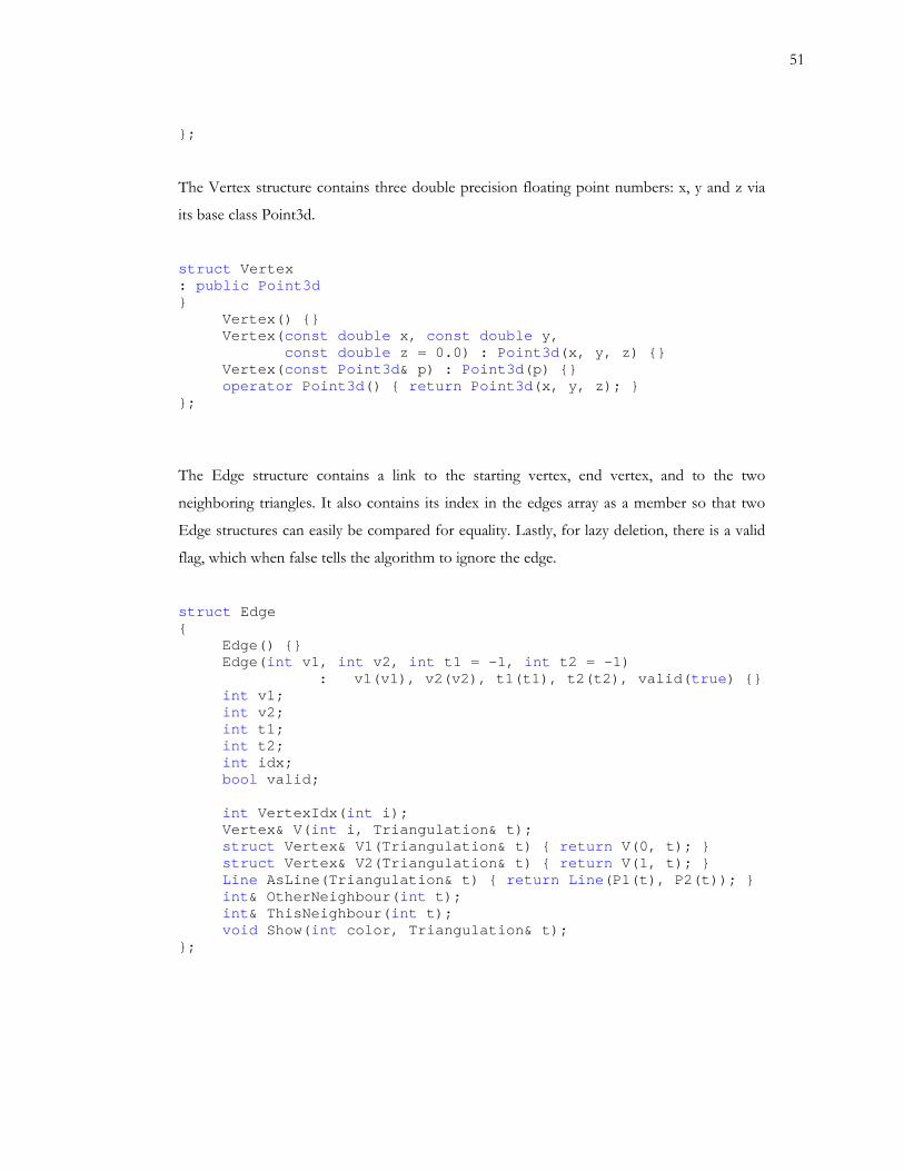
51

};

The Vertex structure contains three double precision floating point numbers: x, y and z via

its base class Point3d.

struct Vertex : public Point3d } Vertex() {} Vertex(const double x, const double y, const double z = 0.0) : Point3d(x, y, z) {}

Vertex(const Point3d& p) : Point3d(p) {} operator Point3d() { return Point3d(x, y, z); }

e Edge str

the edges array as a member so that two

ly be compared for equality. Lastly, for lazy deletion, there is a valid

lls the algorithm to ignore the edge.

= -1) , t2(t2), valid(true) {}

ruct Vert & V1(Tria t); } t); }

};

Th ucture contains a link to the starting vertex, end vertex, and to the two

also contains its index inneighboring triangles. It

Edge structures can easi

flag, which when false te

struct Edge { Edge() {}

Edge(int v1, int v2, int t1 = -1, int t2 : v1(v1), v2(v2), t1(t1)

int v1; int v2; int t1; int t2; int idx; bool valid; int VertexIdx(int i); st ex ngulation& t) { return

Vertex& V(int i, Triangulation& t); V(0,

ngulation& t) { return V(1, struct Vertex& V2(Tria Line AsLine(Triangulation& t) { return Line(P1(t), P2(t)); } int& OtherNeighbour(int t); int& ThisNeighbour(int t); void Show(int color, Triangulation& t); };

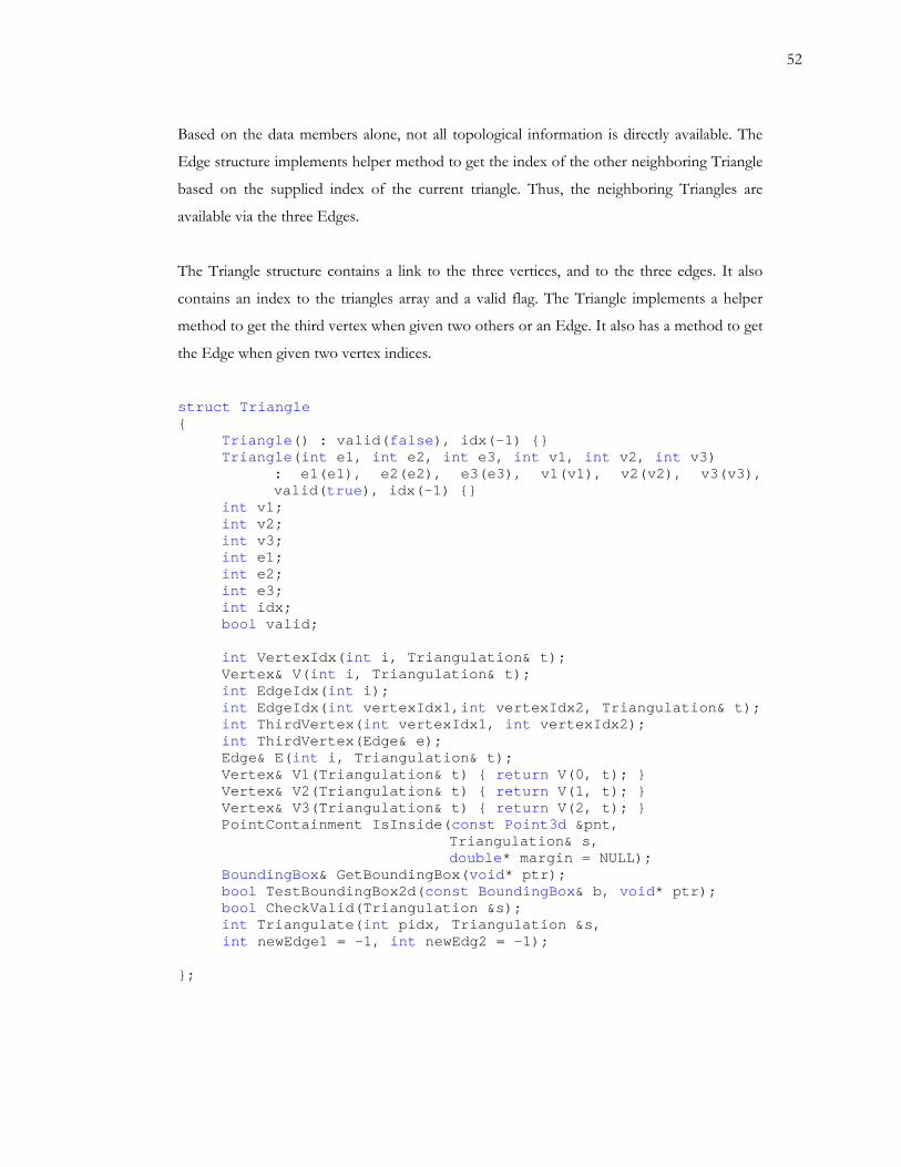
52

Based on the data members alone, not all topological information is directly available. The

dge structure implements helper method to get the index of the other neighboring Triangle

ontains an index to the triangles array and a valid flag. The Triangle implements a helper

int v3; int e1;

rtexIdx(int i, Triangulation& t); V(int i, Triangulation& t);

int EdgeIdx(int i);

PointContainment IsInside(const Point3d &pnt,

int Triangulate(int pidx, Triangulation &s,

E

based on the supplied index of the current triangle. Thus, the neighboring Triangles are

available via the three Edges.

The Triangle structure contains a link to the three vertices, and to the three edges. It also

c

method to get the third vertex when given two others or an Edge. It also has a method to get

the Edge when given two vertex indices.

struct Triangle { Triangle() : valid(false), idx(-1) {} Triangle(int e1, int e2, int e3, int v1, int v2, int v3)

: e1(e1), e2(e2), e3(e3), v1(v1), v2(v2), v3(v3), valid(true), idx(-1) {}

int v1; int v2; int e2; int e3; int idx; bool valid; int Ve Vertex& int EdgeIdx(int vertexIdx1,int vertexIdx2, Triangulation& t); int ThirdVertex(int vertexIdx1, int vertexIdx2); int ThirdVertex(Edge& e); Edge& E(int i, Triangulation& t); Vertex& V1(Triangulation& t) { return V(0, t); } Vertex& V2(Triangulation& t) { return V(1, t); } Vertex& V3(Triangulation& t) { return V(2, t); }

Triangulation& s, double* margin = NULL);

BoundingBox& GetBoundingBox(void* ptr); bool TestBoundingBox2d(const BoundingBox& b, void* ptr); bool CheckValid(Triangulation &s);

int newEdge1 = -1, int newEdg2 = -1); };

53

7.1.2 Triangulation Algorithm

The implemented algorithm is a variant of incremental algorithm (see section 4.1.5).

Although incremental algorithm is not the fastest in many comparisons, it has expected

nning time of Θ(n log n). Because the ability to insert a point or set of points into a

edges are then created via these

ree vertices and added into the triangulation.

e points are added, one by one, into the

iangulation.

return unneeded triangles. Also, some of the

iangles may be marked invalid. Because of this, the found triangles are checked in a loop

and triangles that are either not valid or do not touch the point are discarded.

or each found and accepted triangle a Triangulate function is called. There should be one

ru

Delaunay triangulation was needed anyway, I chose to implement the incremental algorithm.

The algorithm proceeds pretty much as described in 4.1.5. The auxiliary triangle is inserted

first. Its vertices are selected so that the bounding rectangle of the point set is first enlarged

by 10%. Then, the two lower points are added half width of the bounding rectangle away

horizontally from the lower left and right corner of the rectangle. The upper vertex is added

in the horizontally middle, and vertically one half width of the bounding rectangle below the

top of the rectangle. These vertices are added to the end of the vertices array and their

indices are memorized for later removal. A triangle and three

th

As a preliminary check, the point set is tested for duplicates and if there are any, they are

removed. The point set (barring the three auxiliary points) is then shuffled into a random

order to avoid any pathological behavior. Then th

tr

For each point, the triangle quadtree is consulted to find inside which triangle it lies. The

quadtree search is rectangular, and may thus

tr

F

triangle if the point in is inside the triangle, two if the point is on an edge, and several, if the

point is on an edge. The last case should never happen, as there are no duplicates in the

point set. If the point is inside, the Triangulate function divides the triangle into three new

triangles, adding three new edges. The neighboring information is updated and the original

triangle is marked invalid. If the point was on edge, the triangle is divided into two, and three

new edges are added. The old triangle is marked invalid. Triangulate function is called

54

immediately for the triangle that shares the edges the point was on, passing the indices of the

two new common edges as arguments. (If we would just let the loop visit the triangle

plicated edges. The loop will not touch the triangle

ain, since it is marked invalid. The new triangles are also added into the triangle quadtree.)

ller minimum angle among the six corners of the two triangles. If so,

wapDiagonal routine is called. SwapDiagonal routine changes the common edge to go

riangle pair, CheckEdge is called

cursively. As per the description in section 4.1.5, this recursion terminates when the

Delaunay

iangulation, but includes the three auxiliary vertices. As the final step, all the triangles and

edges connected to those three vertices and removed as are the three vertices. Then possible

p.

lookup and recursive CheckEdge function

all. The quadtree lookup is O(log n) for uniform data, and O(n) very badly biased data,

normally, it would result in two new, du

ag

For each new edge created by the triangulation function, CheckEdge routine is called. It

considers the two neighboring triangles of the edges, and checks if swapping the edge would

result in sma

S

between the two other vertices of the two triangles than the ones it originally goes.

Neighboring information is updated, and the two updated triangles are removed and readded

into the quadtree. For each four boundary edges of the t

re

neighborhood of new vertex satisfies the Delaunay criterion.

Once all vertices are inserted into the triangulation, the triangulation is a

tr

concavities are filled with triangles as the last ste

For validation purposes, the implementation also includes a CheckDelaunay function that

goes through all the triangles and using the vertex quadtree checks, if there are any extra

points inside the circumcircle of the triangle.

7.1.3 Complexity Analysis

The algorithm goes through all the points, which is O(n). For each point, two non-constant

time operations are executed: triangle quadtree

c

unless the quadtree is constructed specially or balanced on demand. As per section 4.1.5, the

check edge recursion should terminate in Θ(log n) normal data, but clearly it is O(n) for

biased data. Thus, the overall complexity is O(n2), should be Θ(n log n) for non-biased data.

55

7.1.4 Interpolation Algorithms

The interpolation algorithm is very straight-forward. For point interpolation, the triangle

oint interpolation is O(log n) for uniform data, and O(n) very badly biased data. Polyline

rithm

The implemented system can calculate the volume between two overlapping triangulations.

ion and fill areas as colored areas and as volumes. The user may

so supply a boundary polyline, inside which the calculation is to be done.

gle is then considered one by one. For each triangle, the triangle quadtree

quadtree is consulted to find the triangle the point lies in. If there are several, the first one

will do. The triangle interpolation method described in section 5.8 is then used to get the

height value.

For lines and polylines, the triangle quadtree is consulted to find the triangles that the line or

polyline intersects in 2D. The interpolation is then done as described in section 5.9, and the

result polyline is stitched together from the line segments.

P

interpolation is O(n) since a polyline can touch all the triangles in the triangulation. In

practice, it is usually be Θ(m log n) where m is number of vertices in the polyline.

7.1.5 Volume Calculation Algo

It can give out the excavat

al

The boundaries of the two triangulations are calculated first. This is done by finding the

edges whose other neighbor index is -1. A continuous polyline is then constructed out of

these line segments. Next, the two triangulation boundary polylines and the optional user

supplied one are merged together by taking the 2D intersection of them. The triangulations

are then folded with this united boundary line.

After this, a three dimensional bounding box of the second triangulation is calculated. The

triangle quadtree of the first triangulation is looked up for triangles inside this bounding box.

Every found trian

56

of the second triangulation is looked up for triangles that may collide with this triangle. For

the two triangulations intersect.

Then, both triangulations are again folded with the intersection line segments. After this, we

know that wherever the triangulations intersect, there is an edge and no triangle of either

triangulation may lie partially above and partially below the other triangulation.

After this, we simple go through the triangles in both triangulations calculating the per

triangle volume as described in section 5.10 and add the result into the volume total. For

each triangle, we check if it is under the other triangulation, and add it into the excavation or

fill area and volume respectively.

Because every triangle of either triangulation can potentially intersect several of the other, the

calculation process is pretty heavy. The worst case complexity is in O(m·n) where n is the

amount of triangles in the first triangulation and m is the amount of triangles in the second.

In practice, the triangulations never collide at so many places, and the running time is

tolerable even for large triangulations.

7.2 Environment

The implementation was developed an tested on as an Autocad run-time extension module

(ARX), which closely resembles a DLL, on Windows Vista platform. The Autocad version

used was Autocad Map 2008. Using Autocad allowed me to take advantage of the Autocad

drawing and geometry functionality as well as easily import and export data sets. The source

code was written in C++ and compiled with Microsoft Visual Studio 2005. The

implementation depends on Vianova VidLib geometry library, which implements geometric

primitives such as Point3d, Circle and Triangle (though Triangle was overridden in this

project). The portability was not tested, but the implementation is plain C++, and should be

portable to any other platform apart from the Autocad bindings that are separate from the

calculation core.

every potentially colliding triangle a triangle intersection function is executed and the

potential intersection line segment is added to the array of collision lines. These line

segments form the line where

57

The interpolation, volume calculation and surface intersection parts are part of Vianova

is and is

not (yet) part of any product.

Novapoint products, whereas the triangulation part itself was developed for this thes

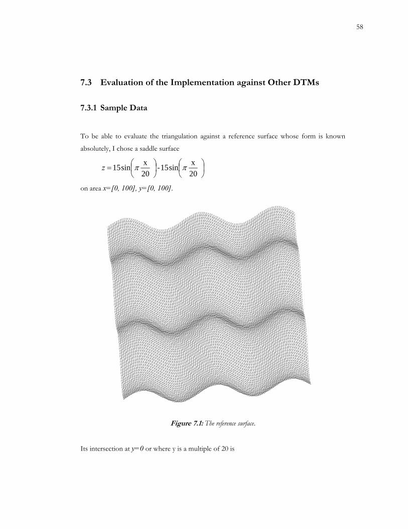
58

To be able to evaluate the triangulation against a reference surface whose form is known

absolutely, I chose a saddle surface

7.3 Evaluation of the Implementation against Other DTMs

7.3.1 Sample Data

⎟⎠⎞

⎜⎝⎛

⎟⎠⎞

⎜⎝⎛=

20xsin15 -

20xsin15 ππz

on area x=[0, 100], y=[0, 100].

Figure 7.1: The reference surface.

Its intersection at y=0 or where y is a multiple of 20 is

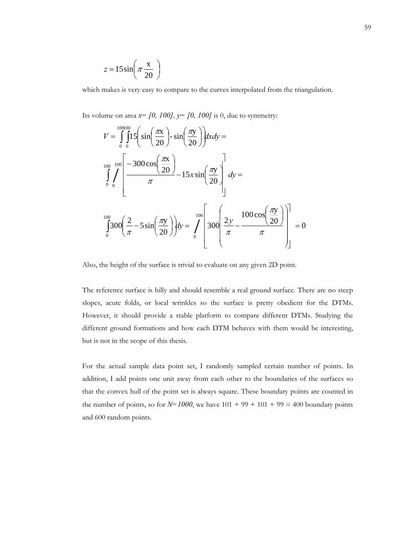
59

20xsin15 ⎟

⎠⎞

⎜⎝⎛= πz

which makes is very easy to compare to the curves interpolated from the triangulation.

Its volume on area x= [0, 100], y= [0, 100] is 0, due to symmetry:

020ycos100

230020ysin52300

20ysin1520

xcos300

20ysin -

20xsin15

/

/

100

0

100

0

100

0

100

0

100

0

100

0

=

⎥⎥⎥⎥

⎦

⎤

⎢⎢⎢⎢

⎣

⎡

⎟⎟⎟⎟

⎠

⎞

⎜⎜⎜⎜

⎝

⎛⎟⎠⎞

⎜⎝⎛

−=⎟⎟⎠

⎞⎜⎜⎝

⎛⎟⎠⎞

⎜⎝⎛−

=

⎥⎥⎥⎥

⎦

⎤

⎢⎢⎢⎢

⎣

⎡

⎟⎠⎞

⎜⎝⎛−

⎟⎠⎞

⎜⎝⎛−

=⎟⎟⎠

⎞⎜⎜⎝

⎛⎟⎠⎞

⎜⎝⎛

⎟⎠⎞

⎜⎝⎛=

∫

∫

∫ ∫

π

π

ππ

π

ππ

π

ππ

ydy

dyx

dxdyV

Also, the height of the surface is trivial to evaluate on any given 2D point.

he reference surface is hilly and should resemble a real ground surface. There are no steep

slopes, acute folds, or local wrinkles so the surface is pretty obedient for the DTMs.

However, it should provide a stable platform to compare different DTMs. Studying the

different ground formations and how each DTM behaves with them would be interesting,

but is not in the scope of this thesis.

For the actual sample data point set, I randomly sampled certain number of points. In

addition, I add points one unit away from each other to the boundaries of the surfaces so

that the convex hull of the point set is always square. These boundary points are counted in

the number of points, so for N=1000, we have 101 + 99 + 101 + 99 = 400 boundary points

and 600 random points.

T

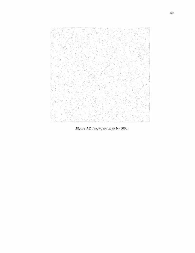
60

Figure 7.2: Sample point set for N=5000.

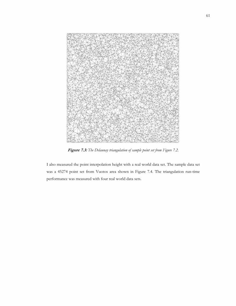
61

Figure 7.3: The Delaunay triangulation of sample point set from Figure 7.2.

th a real world data set. The sample data set

as a 45274 point set from Vuotos area shown in Figure 7.4. The triangulation run-time

I also measured the point interpolation height wi

w

performance was measured with four real world data sets.

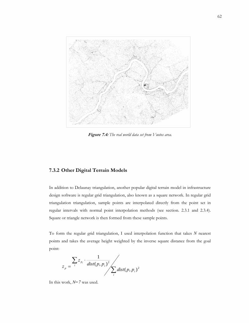
62

Figure 7.4: The real world data set from Vuotos area.

ion, another popular digital terrain model in infrastructure

esign software is regular grid triangulation, also known as a square network. In regular grid

triangulation triangulation, sample points are interpolated directly from the point set in

h normal point interpolation methods (see section. 2.3.1 and 2.3.4).

quare or triangle network is then formed from these sample points.

7.3.2 Other Digital Terrain Models

In addition to Delaunay triangulat

d

regular intervals wit

S

To form the regular grid triangulation, I used interpolation function that takes N nearest

points and takes the average height weighted by the inverse square distance from the goal

point:

∑∑ ⋅

=

ii

i ip

p ppdistppdist

zz

i

2

2

),(),(

1

In this work, N=7 was used.

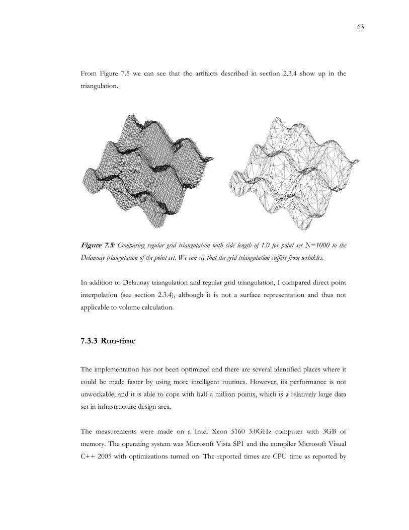
63

From Figure 7.5 we can see that the artifacts described in section 2.3.4 show up in the

triangulation.

Figure 7.5: Comparing regular grid triangulation with side length of 1.0 for point set N=1000 to the

frastructure design area.

Delaunay triangulation of the point set. We can see that the grid triangulation suffers from wrinkles.

In addition to Delaunay triangulation and regular grid triangulation, I compared direct point

interpolation (see section 2.3.4), although it is not a surface representation and thus not

applicable to volume calculation.

7.3.3 Run-time

The implementation has not been optimized and there are several identified places where it

could be made faster by using more intelligent routines. However, its performance is not

unworkable, and it is able to cope with half a million points, which is a relatively large data

set in in

The measurements were made on a Intel Xeon 5160 3.0GHz computer with 3GB of

memory. The operating system was Microsoft Vista SP1 and the compiler Microsoft Visual

C++ 2005 with optimizations turned on. The reported times are CPU time as reported by

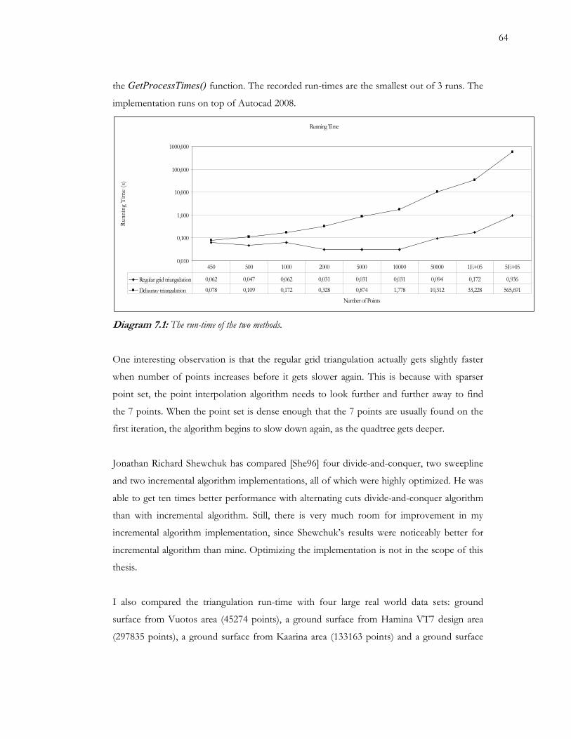
64

the GetProcessTimes() function. The recorded run-times are the smallest out of 3 runs. The

implementation runs on top of Autocad 2008.

Running Time

1,000

10,000

1000,000

Runn

ing

Tim

e (s

100,000

)

0,010

0,100

Regular grid triangulation 0,062 0,047 0,062 0,031 0,031 0,031 0,094 0,172 0,936

Delaunay triangulation 0,078 0,109 0,172 0,328 0,874 1,778 10,312

450 500 1000 2000 5000 10000 50000 1E+05

33,228 565,691

5E+05

Number of Points

et ten times better performance with alternating cuts divide-and-conquer algorithm

an with incremental algorithm. Still, there is very much room for improvement in my

also compared the triangulation run-time with four large real world data sets: ground

rface from Vuotos area (45274 points), a ground surface from Hamina VT7 design area

(297835 points), a ground surface from Kaarina area (133163 points) and a ground surface

Diagram 7.1: The run-time of the two methods.

One interesting observation is that the regular grid triangulation actually gets slightly faster

when number of points increases before it gets slower again. This is because with sparser

point set, the point interpolation algorithm needs to look further and further away to find

the 7 points. When the point set is dense enough that the 7 points are usually found on the

first iteration, the algorithm begins to slow down again, as the quadtree gets deeper.

Jonathan Richard Shewchuk has compared [She96] four divide-and-conquer, two sweepline

and two incremental algorithm implementations, all of which were highly optimized. He was

able to g

th

incremental algorithm implementation, since Shewchuk’s results were noticeably better for

incremental algorithm than mine. Optimizing the implementation is not in the scope of this

thesis.

I

su

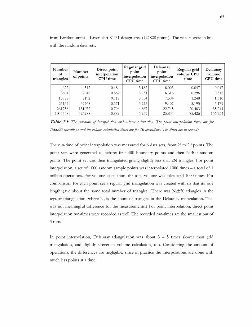
65

from Kirkkonummi – Kivenlahti KT51 design area (127828 points). The results were in line

ith the random data sets.

Table 7.1: The run-time of interpolation and volume calculation. The point interpolation times are for

100000 operations and the volume calculation times are for 10 operations. The times are in seconds.

The run-time of point interpolation was measured for 6 data sets, from 29 to 219 points. The

point sets were generated as before: first 400 boundary points and then N-400 random

points. The point set was then triangulated giving slightly less that 2N triangles. For point

interpolation, a set of 1000 random sample points was interpolated 1000 times – a total of 1

million operations. For volume calculation, the total volume was calculated 1000 times. For

comparison, for each point set a regular grid triangulation was created with so that its side

length gave about the same total number of triangles. (There was Nt±20 triangles in the

regular triangulation, where Nt is the count of triangles in the Delaunay triangulation. This

was not meaningful difference for the measurements.) For point interpolation, direct point

interpolation run-times were recorded as well. The recorded run-times are the smallest out of

3 runs.

ut 3 – 5 times slower than grid

iangulation, and slightly slower in volume calculation, too. Considering the amount of

at a time.

nay

ime

w

Number of

triangles

Number of points

Direct point interpolation

CPU time

Regular grid point

interpolation CPU time

Delaunay point

interpolation CPU time

Regular grid volume CPU

time

Delauvolume

CPU t

In point interpolation, Delaunay triangulation was abo

tr

operations, the differences are negligible, since in practice the interpolations are done with

much less points

622 512 0.484 3.182 8.003 0.047 0.0473694 2048 0.562 3.931 6.318 0.296 0.312

15988 8192 0.718 3.354 7.504 1.248 1.31065134 32768 0.671 3.245 9.407 5.195 5.179

261738 131072 0.796 4.867 22.745 20.483 35.2411045458 524288 0.889 5.959 25.834 85.426 156.734

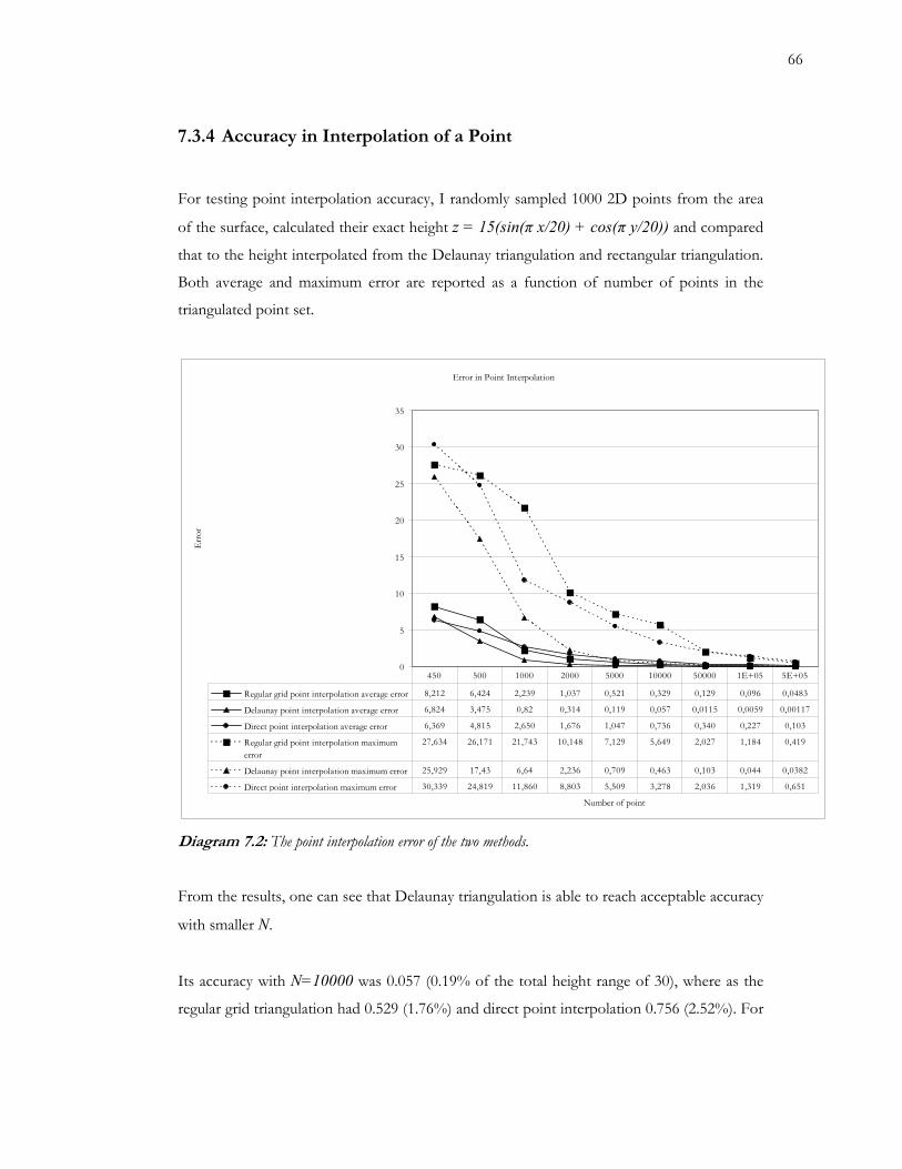
66

7.3.4 Accuracy in Interpolation of a Point

For testing point interpolation accuracy, I randomly sampled 1000 2D points from the area

of the surface, calculated their exact height z = 15(sin(π x/20) + cos(π y/20)) and compared

at to the height interpolated from the Delaunay triangulation and rectangular triangulation. th

Both average and maximum error are reported as a function of number of points in the

triangulated point set.

Error in Point Interpolation

35

Number of point

0

5

10

15

20

25

30

Err

or

Regular grid point interpolation average error 8,212 6,424 2,239 1,037 0,521 0,329 0,129 0,096 0,0483

Delaunay point interpolation average error 6,824 3,475 0,82 0,314 0,119 0,057 0,0115 0,0059 0,00117

Direct point interpolation average error 6,369 4,815 2,650 1,676 1,047 0,736 0,340 0,227 0,103

Regular grid point interpolation maximumerror

27,634 26,171 21,743 10,148 7,129 5,649 2,027 1,184 0,419

Delaunay point interpolation maximum error 25,929 17,43 6,64 2,236 0,709 0,463 0,103 0,044 0,0382

Direct point interpolation maximum error 30,339 24,819 11,860 8,803 5,509 3,278 2,036 1,319 0,651

5E+05450 500 1000 2000 5000 10000 50000 1E+05

Its accuracy with N=10000 was 0.057 (0.19% of the total height range of 30), where as the

regular grid triangulation had 0.529 (1.76%) and direct point interpolation 0.756 (2.52%). For

Diagram 7.2: The point interpolation error of the two methods.

From the results, one can see that Delaunay triangulation is able to reach acceptable accuracy

with smaller N.

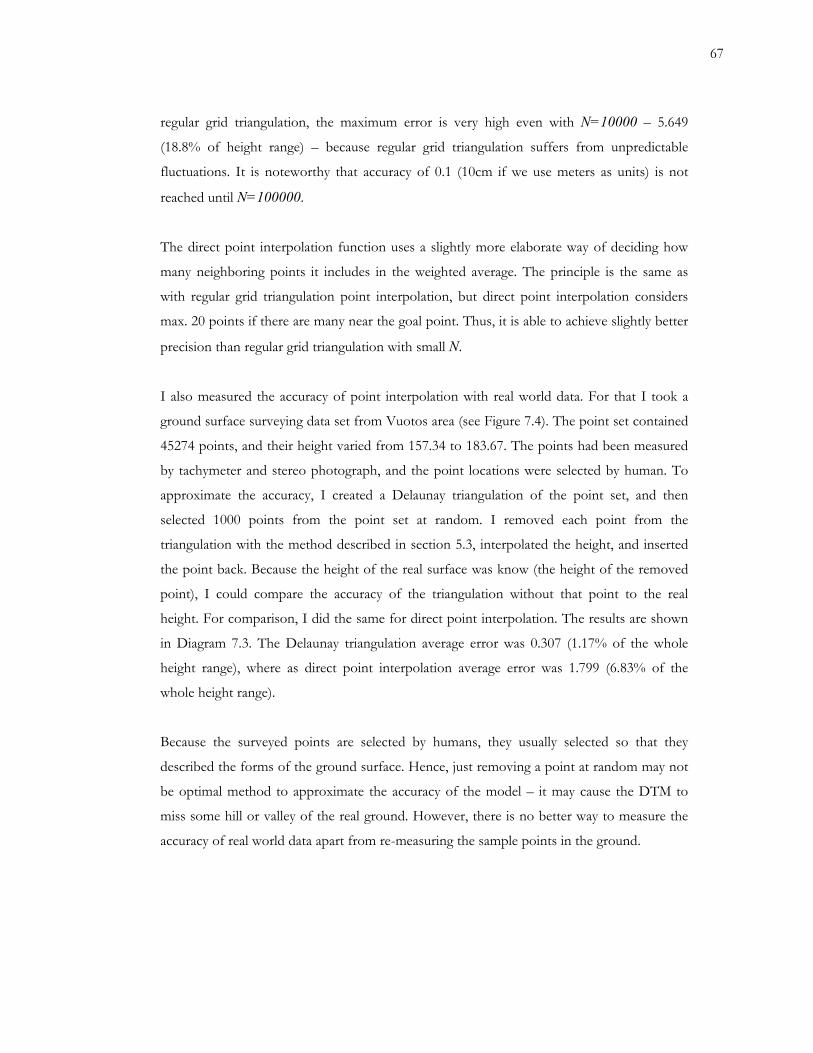
67

regular grid triangulation, the maximum error is very high even with N=10000 – 5.649

(18.8% of height range) – because regular grid triangulation suffers from unpredictable

fluctuations. It is noteworthy that accuracy of 0.1 (10cm if we use meters as units) is not

reached until N=100000.

The direct point interpolation function uses a slightly more elaborate way of deciding how

many neighboring points it includes in the weighted average. The principle is the same as

with regular grid triangulation point interpolation, but direct point interpolation considers

max. 20 points if there are many near the goal point. Thus, it is able to achieve slightly better

precision than regular grid triangulation with small N.

I also measured the accuracy of point interpolation with real world data. For that I took a

ground surface surveying data set from Vuotos area (see Figure 7.4). The point set contained

45274 points, and their height varied from 157.34 to 183.67. The points had been measured

by tachymeter and stereo photograph, and the point locations were selected by human. To

approximate the accuracy, I created a Delaunay triangulation of the point set, and then

selected 1000 points from the point set at random. I removed each point from the

ed the height, and inserted

e point back. Because the height of the real surface was know (the height of the removed

point), I could compare the accuracy of the triangulation without that point to the real

terpolation. The results are shown

Diagram 7.3. The Delaunay triangulation average error was 0.307 (1.17% of the whole

om may not

be optimal method to approximate the accuracy of the model – it may cause the DTM to

miss some hill or valley of the real ground. However, there is no better way to measure the

accuracy of real world data apart from re-measuring the sample points in the ground.

triangulation with the method described in section 5.3, interpolat

th

height. For comparison, I did the same for direct point in

in

height range), where as direct point interpolation average error was 1.799 (6.83% of the

whole height range).

Because the surveyed points are selected by humans, they usually selected so that they

described the forms of the ground surface. Hence, just removing a point at rand

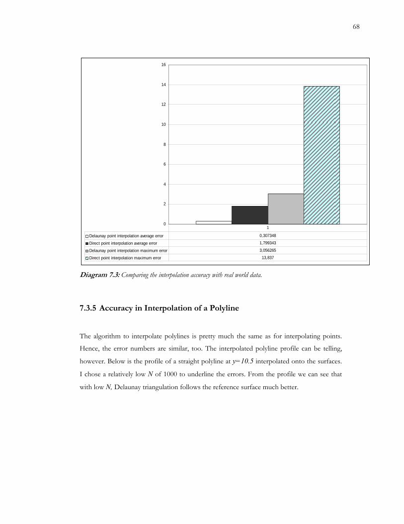
68

0

2

4

6

8

10

12

14

16

Delaunay point interpolation average error 0,307348

Direct point interpolation average error 1,799343

Delaunay point interpolation maximum error 3,056265

13,837

1

Direct point interpolation maximum error

Comparing the interpolation accuracy with real world data.

he algorithm to interpolate polylines is pretty much the same as for interpolating points.

Hence, the error numbers are similar, too. The interpolated polyline profile can be telling,

however. Below is the profile of a straight polyline at y=10.5 interpolated onto the surfaces.

I chose a relatively low N of 1000 to underline the errors. From the profile we can see that

with low N, Delaunay triangulation follows the reference surface much better.

Diagram 7.3:

7.3.5 Accuracy in Interpolation of a Polyline

T

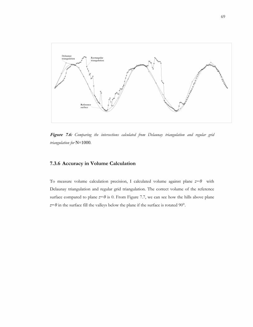
69

Figure 7.6: Comparing the intersections calculated from Delaunay triangulation and regular grid

triangulation for N=1000.

.3.6 Accuracy in Volume Calculation 7

To measure volume calculation precision, I calculated volume against plane z=0 with

Delaunay triangulation and regular grid triangulation. The correct volume of the reference

surface compared to plane z=0 is 0. From Figure 7.7, we can see how the hills above plane

z=0 in the surface fill the valleys below the plane if the surface is rotated 90°.

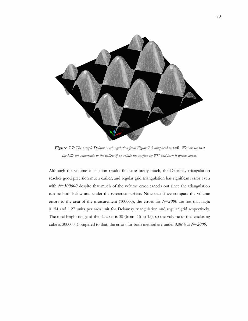
70

Figure 7.7: The sample Delaunay triangulation from Figure 7.3 compared to z=0. We can see that

the hills are symmetric to the valleys if we rotate the surface by 90° and turn it upside down.

Although the volume calculation results fluctuate pretty much, the Delaunay triangulation

reaches good precision much earlier, and regular grid triangulation has significant error even

e

of the measurement (100000), the errors for N=2000 are not that high:

with N=500000 despite that much of the volume error cancels out since the triangulation

both below and under the reference surface. Note that if we compare the volumcan be

errors to the area

0.154 and 1.27 units per area unit for Delaunay triangulation and regular grid respectively.

The total height range of the data set is 30 (from -15 to 15), so the volume of the. enclosing

cube is 300000. Compared to that, the errors for both method are under 0.06% at N=2000.

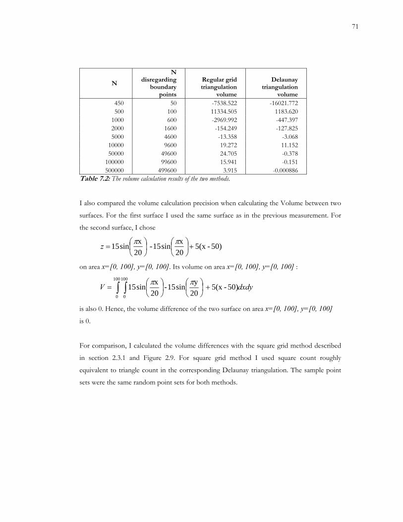
71

N

Nding

boundary oints

egular gtriangulat

volume

Deltriangulation

volum

Rdisregar

p

rid ion

aunay

e 450 50 -16021.-7538.522 772 500 100 1334.505 1183.620 1

1000 600 -447.397 -2969.992 2000 1600 -154.249 -127.825 5000 4600 -13.358 -3.068

10000 9600 19.272 11.152 50000 49600 24.705 -0.378

100000 99600 15.941 -0.151 500000 499600 3.915 -0.000886

Table 7.2: The volume calculation results of the two methods.

I also compared the volume calculation precision when calculating the Volume between two

surfaces. For the first surface I used the same surface as in the previous measurement. For

the second surface, I chose

50) -5(x 20xsin15 -

20 ⎠⎝

xsin15 +⎟⎠⎞

⎜⎝⎛

⎟⎞

⎜⎛=

ππz

rea x=[0, 100], y=[0, 100]. Its volume on area x=[0, 100], y=[0, 100] : on a

dxdyV ∫ ∫ +⎟⎠⎞

⎜⎝⎛

⎟⎠⎞

⎜⎝⎛=

100

0

100

0

50) -5(x 20ysin15 -

20xsin15 ππ

is also 0. Hence, the volume difference of the two surface on area x=[0, 100], y=[0, 100]

is 0.

For comparison, I calculated the volume differences with the square grid method described

in section 2.3.1 and Figure 2.9. For square grid method I used square count roughly

equivalent to triangle count in the corresponding Delaunay triangulation. The sample point

sets were the same random point sets for both methods.

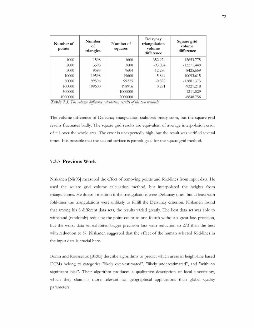
72

Number of Number

of s

Number of squares

Delaynay triangulation

volume difference

Square grid volume

difference points

triangle

1000 1598 1600 352.974 12653.775 2000 3598 3600 -93.084 -12271.448 5000 9598 9604 -12.280 -8425.669

10000 19598 19600 5.849 10093.615 50000 99596 99225 -0.892 -12881.373

100000 199600 198916 0.281 -9321.218 500000 1000000 -1211.029

1000000 2000000 -8848.756 Table 7.3: The volume difference calculation results of the two methods.

The volume difference of Delaunay triangulation stabilizes pretty soon, but the square grid

results fluctuates badly. The square grid results are equivalent of average interpolation error

f ~1 over the whole area. The error is unexpectedly high, but the result was verified several

iangulations were Delaunay ones, but at least with

ld-lines the triangulations were unlikely to fulfill the Delaunay criterion. Niskanen found

effect of the human selected fold-lines in

e input data is crucial here.

parameters.

o

times. It is possible that the second surface is pathological for the square grid method.

7.3.7 Previous Work

Niskanen [Nis93] measured the effect of removing points and fold-lines from input data. He

used the square grid volume calculation method, but interpolated the heights from

triangulations. He doesn’t mention if the tr

fo

that among his 8 different data sets, the results varied greatly. The best data set was able to

withstand (randomly) reducing the point count to one fourth without a great loss precision,

but the worst data set exhibited bigger precision loss with reduction to 2/3 than the best

with reduction to ¼. Niskanen suggested that the

th

Bonin and Rousseaux [BR05] describe algorithms to predict which areas in height-line based

DTMs belong to categories "likely over-estimated", "likely underestimated", and "with no

significant bias". Their algorithm produces a qualitative description of local uncertainty,

which they claim is more relevant for geographical applications than global quality

73

8 Conclusion

to

implement and they have low run-time cost.

This Master’s Thesis has described various digital terrain models and how Delaunay

triangulation compares to them. I have discussed various theoretical properties of the

Delaunay triangulation and how they are desirable for infrastructure design applications. I

have outlined several ways to construct a Delaunay triangulation, and described one

Delaunay triangulation algorithm implementation in detail and the challenges in

implementing it. I have also described how Delaunay triangulation can be used to point and

polyline interpolation and to volume calculation, which are the most important infrastructure

design application operations for DTMs.

I have measured the running-time of the implementation and compared it to two other

DTM variants in both constructing the DTM and using it for interpolation and volume

calculations. I have measured the accuracy of the DTM variants with ideal and real world

data sets in interpolation and volume calculation.

The measurements show that the accuracy of Delaunay triangulation in infrastructure design

application – in particular, point interpolation and volume calculation – is good, and it

doesn’t suffer from unpredictable spikes. The Delaunay triangulation achieves good accuracy

with considerable smaller amount of input data, which translates into smaller costs in

surveying the ground surface. With modern hardware, its run-time performance is

The main concerns in modeling surface in infrastructure design software arise from the high

accuracy and correctness needs of the application domain. Errors in the calculations may not

only cause large costs and delays, but also expose the built structure to the risk of collapsing.

On the other hand, the surveying the surface to get high number of accurate sample points is

costly and slow. Therefore, it is crucial that the digital terrain model constructed from the

sample points is as good as possible. Traditionally, the infrastructure design software

packages have used simple grid base surface approximations because they are easy

74

comparable to other methods, and in practice, it is not the bottle-neck of the design process.

The small performance penalty is easily won back in shorter surveying time.

tructure design software available commercially today still uses DTMs other

than Delaunay triangulation for interpolation and volume calculation. Based on this research,

because they would h

triangulation algorithm n paper – are pretty complex and laborous to

implement in practice ler

DTMs. These proble he work invested in perfecting the

y triangulation

A part of infras

this can only be because they are easier to implement than Delaunay triangulation, not

ave other desirable properties. Based on my experience, the Delaunay

s – while simple o

. They are also more prone to implementation bugs that the simp

ms are not insurmountable, and t

Delauna implementations should not be high compared to the advantages.

75

References

[Bar07]

ynergistic processing elements of the Sony

xps3-

Jonathan Bartlett. Programming high-performance applications on the Cell BE

processor, Part 2: Program the s

PLAYSTATION 3.

http://www.ibm.com/developerworks/power/library/pa-linu

2/index-a4.pdf as of 06.01.2009.

[BDH96] C. Bradford Barber, David P. Dobkin, Hannu Huhdanpaa. The

quickhull algorithm for convex hulls. In ACM Transactions on

Mathematical Software (TOMS)

archive Volume 22, Issue 4. Pages: 469-

483. 1996. http://portal.acm.org/citation.cfm?id=235815.235821 as

of 10.01.2009.

[BR05] Frederic Rousseaux. Digital Terrain Model

[DEM95] Dickerson, Scott A. McElfresh, Mark Motangue. New

, 1995.

[BKOS97] M. de Berg, M. Van Kreveld, M. Overmars, O. Schwarzkopf.

Computational Geometry, Algorithms and Applications. Springer 1997.

Olivier Bonin

Computation from Contour Lines: How to Derive Quality

Information from Artifact Analysis. In

Geoinformatica archive Volume 9, Issue 3 (September 2005). Pages 253-

268.

Matthew T.

Algorithms and Empirical Findings on Minimum Weight

Triangulation Heuristics. In Proceedings of the Eleventh Annual Symposium

on Computational Geometry. Pages 238 – 247. ACM Press

http://portal.acm.org/citation.cfm?id=220305 as of 08.01.2009.

Matthew T. Dickerson, Robert L. Scot Drysdale, Scott A. McElfresh,

Emo Welzl. Fast greedy triangulation algorithms. In Proceedings of the

tenth annual symposium on Computational geometry. Pages: 2

[DDMW94]

11-220. 1994.

http://portal.acm.org/citation.cfm?id=177424.177649 as of

09.01.2009.

76

[Dwye86 Rex Dwyer. A simple divide-and-conquer algorithm for computing

Delaunay triangulations in O(n log log n) expected time. In Proceedings

of the second annual symposium on Computational geometry. 1986.

]

http://portal.acm.org/citation.cfm?id=10515.10545 as of 26.12.2008.

[Eber02] David Eberly. Triangulation by Ear Clipping.

http://www.geometrictools.com/Documentation/TriangulationByEa

rClipping.pdf as of 24.12.2008.

[For92]

s. In Proceedings of the eighth annual symposium on computational

[For87] Steven Fortune. A Sweepline Algorithm for Voronoi Diagrams. In

Algorithmica Vol 2, Number 2, 153-174. Springer-Verlag 1987.

http://portal.acm.org/citation.cfm?id=10515.10549 as of 09.01.2009.

Steven Fortune. Numerical stability of algorithms for 2D Delaunay

triangulation

geometry. Pages 83-92. 1992.

http://portal.acm.org/citation.cfm?id=142675.142695 as of

10.01.2009

[GICPE07] , Jaime Puig-Pey, Jesús

imation.

tent/y24516n216x6820k/

[For96] Steven Fortune. Robustness in Geometric Algorithms. In Applied

Computational Geometry: Towards Geometric Engineering, pages 7-14,

Springer 1996.

Akemi Gálvez, Andrés Iglesias, Angel Cobo

Espinola. Bézier Curve and Surface Fitting of 3D Point Clouds Through

Genetic Algorithms, Functional Networks and Least-Squares Approx

http://www.springerlink.com/con as of

[GKS92] ibas, Donald E. Knuth, Micha Sharir. Randomized

ger-Verlag.

the twentieth annual

l.acm.org/citation.cfm?id=997817.997846

15.12.2008.

Leonidas J. Gu

Incremental Construction of Delaunay and Voronoi Diagrams. In

Algorithmica (1992) 7. Pages 381-413. Sprin

[GR04] Leonidas Guibas, Daniel Russel. An empirical comparison of

techniques for updating Delaunay triangulations. In Annual Symposium

on Computational Geometry archive Proceedings of

symposium on Computational geometry. Pages 170-179. 2004.

http://porta as of

02.01.2009.

77

[GS85]

Computation of Voronoi Diagrams. In

m.org/citation.cfm?id=282923

Leonidas Guibas, Jorge Stolfi. Primitives for the Manipulation of

General Subdivisions and the

ACM Transactions on Graphics 4(2). Pages 75-123. 1985.

http://portal.ac as of 09.01.2009.

lation algorithm. In SPAA '97: Proceedings of

//portal.acm.org/citation.cfm?id=258492.258516

[Gui96] Leonidas J. Guibas. Implementing Geometric Algorithms Robustly. In

Applied Computational Geometry: Towards Geometric Engineering, pages 15-

22, Springer 1996.

[Har97] Jonathan C. Hardwick. Implementation and evaluation of an efficient

parallel Delaunay triangu

the ninth annual ACM symposium on Parallel algorithms and architectures June

1997. http: as of

[HD06] on series:

er Berlin Heidelberg

[HLS93] er, Larry L. Schumaker. Fundamentals of

[Hop96]

rosoft.com/en-us/um/people/hoppe/pm.pdf

06.02.2009.

Øyvind Hjelle, Morten Dæhlen. Mathematics and Visualizati

Triangulations and Applications. Pages 73-93. Spring

2006.

[HHKL09] Heikki Halttula, Tuomas Hörkkö, Juha Kajanen, Juha Liukas, Jarmo

Muukkonen, Tuomas Peltonen, Juho Siipo, Jarkko Sireeni, Timo

Vikström. IT-pohjainen infrasuunnittelu (IT-Based Infrastructure Design).

Rakennusteollisuuden Kustannus RTK. 2009.

Josef Hoschek, Dieter Lass

Computer-aided Geometric Design. Pages 295-301. A K Peters, Ltd.

Hugues Hoppe. Progressive meshes.

http://research.mic as

[HW99]

[ILSS06] nxin Liu, Jonathan Shewchuk, Jack Snoeyink.

of 27.12.2008.

Lennart Håde, Bertil Westergren. Mathematics Handbook for Science and

Engineering. 4th ed. Springer-Verlag. 1999.

Martin Isenburg, Yua

Streaming computation of Delaunay triangulations. In ACM

SIGGRAPH 2006 Papers. Pages 1049-1056. 2006.

http://portal.acm.org/citation.cfm?id=1179352.1141992 as of

10.01.2009.

[IM08] Rakennusteollisuus, Liikenne- ja viestintäministeriö,

Ratahallintokeskus, Suomen Kuntaliitto, Suomen Maarakentajien

78

Keskusliitto, Tekes, Tiehallinto. Infra 2010 -ohjelman esiselvitys (Pre-

report on Infra 2010 Project).

isto/Infra%202010%20raportti.pdfhttp://www.infra2010.fi/Aine as

[JK01]

. In Maankäyttö

[KK03]

riterion.

of

[Knu98] Art of Computer Programming, Volume 3, Sorting

[LM08] LandXML.org. LandXML-1.2 specification.

of 21.12.2008.

Jarkko Koski. Laserkeilaus – Uusi ulottuvuus tiedon keräämiseen (Laser

Scanning – A New Dimension to Data Gathering)

magazine 04/2001.

Josef Kohout, Ivana Kolingerová. Parallel Delaunay Triangulation Based

on Circum-Circle C

http://portal.acm.org/citation.cfm?id=984952.984966 as

06.01.2009.

Donald E Knuth. The

and Searching. Page 565- 566. 2nd Ed. Addison-Wesley. 1998.

http://www.landxml.org/spec.htm as of 21.12.2008.

A. Mirante, N. W[MW82] eingarten. The Radial Sweep algorithm for

09/MCG.198

constructing triangulated irregular networks. IN IEEE Computer

Graphics and Applications, 2(3). Pages 11-21. 1982.

http://www2.computer.org/portal/web/csdl/doi/10.11

2.1674214 as of 08.01.2009.

Niskane[Nis93] Jari n. Digitaalisen massalaskennan tarkkuus (The accuracy of

[Nur02] Nurminen, Kimmo. Digitaalisten ilmakuvien käyttö kaupungin

[MR08]

nal of the ACM (JACM) archive Volume 55, Issue 2 (May

digital volume calculation), Master’s Thesis. Tampere University of

Technology. 1993.

paikkatietojärjestelmässä (Digital Aerial Photographs in Municipal

Geographic Information System), Master’s Thesis. Helsinki University

of Technology. 2002.

Wolfgang Mulzer, Günter Rote. Minimum-weight triangulation is NP-

hard. In Jour

2008). http://portal.acm.org/citation.cfm?id=1346330.1346336 as of

08.01.2009.

Atul Narkhede, Dinesh Manocha. Fast Polygon Triangulation based on

Seidel's Algorithm. Department of Computer Science, UNC Chapel Hill.

[NM95]

79

http://www.cs.unc.edu/~dm/CODE/GEM/chapter.html as of

24.12.2008 or

http://www.iut-arles.up.univ-

mrs.fr/raffin.r/myspip/fichiers_static/lpin/reflexions2008/Fast%20p

olygon%20triangulation%20based%20on%20Seidel%20algorithm_Gr

aphics%20Gems%20V_pp401.pdf as of 24.12.2008.

[Pre96]

Towards Geometric Engineering, pages 23-24,

[PT97]

[PP98] G.Pinelli. A Ground Penetrating Radar for Soil

Pattern Recognition.

http://www.idscompany.it/upload4/File/Igarss98.pdf

Franco P. Preparata. Robustness in Geometric Algorithms. In Applied

Computational Geometry:

Springer 1996.

Les A. Piegl, Wayne Tiller. The NURBS Book. Springer. 1997.

G. De Pasquale,

as of

13.12.2008.

[Rour98] Joseph O'Rourke. Computational Geometry in C. Cambridge University

Press. 1998.

[RTCS07] Guodong Rong, Tiow-Seng Tan, Thanh-Tung Cao, Stephanus (sic).

Computing Two-dimensional Delaunay Triangulation Using Graphics Hardware.

School of Computing National University of Singapore.

http://portal.acm.org/citation.cfm?id=1342250.1342264 as of

07.01.2009.

[Rup95] Jim Ruppert. A Delaunay Refinement Algorithm for Quality 2-

Dimensional Mesh Generation. In Journal of Algorithms 18(3):548-585,

May 1995.

[SD95] Peter Su, Robert L. Scot Drysdale. A comparison of Sequential

Delaunay Triangulation Algorithms. In Proceedings of the Eleventh Annual

Symposium on Computational Geometry, 61-70. ACM 1995.

http://portal.acm.org/citation.cfm?id=220279.220286 as of

08.01.2009.

[She96] Jonathan Richard Shewchuk. Triangle: Engineering a 2D Quality Mesh

Generator and Delaunay Triangulator. In Applied Computational

Geometry: Towards Geometric Engineering Engineering, volume 1148 of

Lecture Notes in Computer Science. Pages 203-222. Springer-Verlag.

80

1996. HTUhttp://www.cs.berkeley.edu/~jrs/papers/triangle.pdfUTH as of

06.01.2009.

[THMPG03] Matthias Teschner, Bruno Heidelberger, Matthias Müller, Danat

Pomeranets, Markus Gross. Optimized Spatial Hashing for Collision

Detection of Deformable Objects. Computer Graphics Laboratory, ETH

Zurich.

HTUhttp://www.beosil.com/download/CollisionDetectionHashing_VMV

03.pdfUTH as of 09.01.2009.

[VB04] James M. van Verth, Lars M. Bishop. Essential Mathematics for Games &

Interactive Applications – A Programmer’s Guide. Morgan Kaufmann

Publishers 2004.