Using Contour Trees in the Analysis and Visualization of RadioAstronomy Data Cubes

Paul Rosen*

University of South FloridaBei Wang†

University of UtahAnil Seth ‡

University of UtahBetsy Mills §

San Jose State University

Adam Ginsburg ¶

National Radio Astronomy ObservatoryJulia Kamenetzky ||

Westminster CollegeJeff Kern **

National Radio Astronomy Observatory

Chris R. Johnson††

University of Utah

Figure 1: The results of varying the simplification level on slice #18 of the Ghost of Mirach dataset using a 2D contour tree. On thetop left, a visualization of the original data is shown. On the bottom left, the contour tree computed on the region is shown withcircles at critical point locations. Finally, on the right, the results of simplifying the data with simplification levels of 0.0005, 0.001,0.0015, 0.002, from left to right, top to bottom, respectively.

ABSTRACT

The current generation of radio and millimeter telescopes, particu-larly the Atacama Large Millimeter Array (ALMA), offers enormousadvances in observing capabilities. While these advances representan unprecedented opportunity to advance scientific understanding,the increased complexity in the spatial and spectral structure of evena single spectral line is hard to interpret. The complexity present incurrent ALMA data cubes therefore challenges not only the exist-ing tools for fundamental analysis of these datasets, but also users’ability to explore and visualize their data. We have performed afeasibility study for applying forms of topological data analysis and

*e-mail: prosen@usf.edu†e-mail: beiwang@sci.utah.edu‡e-mail: aseth@astro.utah.edu§e-mail: elisabeth.mills@sjsu.edu¶e-mail: aginsbur@aoc.nrao.edu||e-mail: jkamenetzky@westminstercollege.edu

**e-mail: jkern@nrao.edu††e-mail: crj@sci.utah.edu

visualization never before tested by the ALMA community. Throughcontour tree-based data analysis, we seek to improve upon existingdata cube analysis and visualization workflows, in the forms of im-proved accuracy and speed in extracting features. In this paper, wereview our design process in building effective analysis and visu-alization capabilities for the astrophysicist users. We summarizeeffective design practices, in particular, we identify domain-specificneeds of simplicity, integrability and reproducibility, in order to besttarget and service the large astrophysics community.

1 INTRODUCTION

Radio astronomy is currently undergoing a revolution driven bynew high spatial and spectral resolution observing capabilities. Thecurrent generation of radio and millimeter telescopes, particularlythe Atacama Large Millimeter Array (ALMA), offers enormousadvances in capabilities, including significantly increased sensitivity,resolution, and spectral bandwidth. While these advances representan unprecedented opportunity to advance scientific understanding,they also pose a significant challenge. In some cases, the higher sen-sitivity and resolution they provide yield new detections of sourceswith well-ordered structure that is easy to interpret using currenttools (e.g., HL Tau [41]). However, these advances equally oftenlead to the detection of structure with increased spatial and spectralcomplexity (e.g., new molecules in the chemically-rich massive star

arX

iv:1

704.

0456

1v1

[as

tro-

ph.I

M]

15

Apr

201

7

forming region Sgr B2, outflows in the nuclear region of the nearbygalaxy NGC 253, and rich kinematic structure in the giant molecu-lar cloud “The Brick” [8, 10, 47]). The new complexity present incurrent spectral line datasets challenge not only the existing toolsfor fundamental analysis of these datasets, but also users’ ability toexplore and visualize their data.

1.1 ContributionInspired by Topological Data Analysis (TDA), we perform a fea-sibility study for applying forms of data analysis and visualizationnever before tested by the ALMA community. Through contourtree-based techniques, we seek to improve upon existing data cubeanalysis and visualization, in the forms of improved accuracy andspeed in finding and extracting features.

We present the resulting software, called ALMA-TDA (https://github.com/SCIInstitute/ALMA-TDA), which uses contourtrees to extract and simplify the complex signals from noisy radioastronomy data, commonly refereed to as ALMA data cubes. ALMAis an astronomical interferometer of radio telescopes located innorthern Chile; it delivers data cubes (sometimes referred to asposition-position-frequency cubes), of which the first two axes arepositions and the third axis is the frequency or spectral domain.

An example of our tool is seen in Figure 1. In this figure, theoriginal noisy data is shown on the upper left. The lower left showsthe critical points extracted by the contour tree. Finally, the fourimages to the right show differing levels of simplification of the data.

In this paper, we review our design process in building effec-tive analysis and visualization capabilities for ALMA data cubes.We summarize effective design practices targeting and servicingthe large astrophysics community, in particular, we need to designtools with simplicity (i.e., light-weight), integrability (i.e., integrablewithin existing tool chains) and reproducibility (i.e., fully recordedanalysis history via command-lines). We hope such learned designpractices will provide guidelines toward future development of toolsand techniques that would benefit astrophysicists’ scientific goals.

2 SCIENCE CASE

The new complexity brought about by increased sensitivity, spatialand spectral resolution, and spectral bandwidth has become a signif-icant bottleneck in science, as it not only challenges astrophysicists’analysis tools but also the users’ ability to understand their data. Forexample, increased complexity in the spatial and velocity structureof spectral line emission makes even a single spectral line hard tointerpret. When a cube contains the superposition of multiple spatialand kinematic structures, such as outflows and rotation and infall,each with their own relationship between the observed velocity andtheir actual position along the line of sight, traditional analysis andexploration tools fail. Users struggle to follow kinematic trendsacross multiple structures by examining movies or channel maps ofthe data. However, moment map analysis (e.g., integrated fluxes,mean velocities and mean line-widths), the most commonly usedanalysis tool for compressing this 3D information into a more easilyparsed 2D form, no longer has a straightforward interpretation in thepresence of such complex structure, in which mean velocities maybe velocities at which no emission is actually present, and mean linewidths may represent the distance between two velocity components,rather than the width of a single component.

Whether scientists can navigate and correctly interpret this newcomplexity will determine their success in addressing a numberof important scientific questions. Among the topics driven by thedetection of more complex structures are ISM turbulence [21,48], thestar formation process [31], filaments [45], molecular cloud structureand kinematics [47], and the kinematics of nearby galaxies [29, 30,34] and high redshift galaxies [42, 55].

An even greater challenge arises from our ability to detect anincreased number of spectral lines in more and more sources. There

simply are no tools capable of simultaneously visualizing, compar-ing, and analyzing the dozens to hundreds of data cubes for all of thedetected spectral lines in a given source. Such standard methods ofboth visualizing and exploring data as moment maps, channel maps,playing cube like a video, or 3D models, cannot scale up to the caseof large numbers of lines, even in non-complex, well-ordered cases,such as rotating disks, or expanding stellar shells. Users becomeoverwhelmed by, for example, comparing these typical diagnosticsfor two lines, side by side or one at a time. In the richest sources withthousands of lines, such comparisons will simply be impossible—itbecomes necessary to resort to methods that entirely throw awayeither the spectral information such as Principle Component Analy-sis (PCA) of moment maps or the spatial information that requiresmodel fitting of complex spectra. As a result, both exploration andanalysis of the data becomes not only time consuming, but poten-tially incomplete.

As we move into the future and these telescopes reach their fullpotential, complex spatial and velocity structure will no longer bea problem that typically occurs in a separate subset of sources thanthose exhibiting rich spectra—the two problems will coexist, com-pounding the highlighted issues. The visualization and analysischallenges currently facing radio astronomy will then only growmore pressing as instruments grow more sensitive and the data vol-umes become larger.

2.1 Existing Tools

A critical aspect to the study of ALMA data cubes is the detection,extraction and characterization of objects such as stars, galaxies,and blackholes. Source finding in radio astronomy is the process ofdetecting and characterizing objects in radio images (in the forms ofdata cubes), and returning a survey catalogue of the extracted objectsand their properties [27,56]. A common practice is to use a computerprogram (i.e., a source finder) to search the data cubes, followed bymanual inspection to confirm the sources of electromagnetic radia-tion [56]. An ideal source finder aims to determine the location andproperties of these astronomical objects in a complete and reliablefashion [27]; while manual inspection is often time-consuming andexpensive.

Several existing tools have been used in the ALMA communityin terms of source finding [28], including the popular ones such asclumpfind [57], dendrograms [51], cprops [50], and more recentones such as FellWalker [9], SCIMES [20] and NeuroScope [35].Clumpfind is designed for analyzing radio observations of molecularclouds obtained as 3D data cubes, it works by contouring the data,searching for local peaks of emission and following them down tolower intensity levels [57]. The dendrograms of a data cube is anabstraction of the changing topology of the isosurfaces as a func-tion of contour level, which captures the essential features of thehierarchical structure of the isosurfaces [51]. The FellWalker algo-rithm is a gradient-tracing watershed algorithm that segment imagesinto regions surrounding local maxima [9]. FellWalker providessome ability to merging clumps, therefore simplify the underly-ing structures, and the merging criteria shares some similaritieswith persistence-based simplification. However these criteria areless mathematical rigorous compared to our approach. SCIMES(Spectral Clustering for Interstellar Molecular Emission Segmen-tation) considers the dendrogram of emission under graph theoryand utilizes spectral clustering to find discrete regions with similaremission properties [20]. Finally, the most recent NeuroScope [35](specifically targeted for ALMA data cubes) employs a set of neuralmachine learning tools for the identification and visualization ofspatial regions with distinct patterns of motion.

However, the study of source finding for ALMA data cubes raisesthe following question: How can we help the astrophysicists tounderstand the de-noising process? That is, how to best separatesignals from noise, and the effects of de-noising on the original data?

In other words, it is important for us to quantify both signals andnoise as well as to perform simplifications of the underline data.This kind of study is underdeveloped with current approaches in theALMA community .

3 TECHNICAL BACKGROUND: CONTOUR TREES

From a technical perspective, we focus on performing data analysisand designing effective visualization of ALMA data cubes by em-ploying the contour tree [13]. The contour tree is a mathematicalobject describing the evolution of the level sets of a scalar functiondefined on a simple, connected domain, such as the grayscale in-tensity defined on the 2D domain associated with a slice of a datacube (at a fixed frequency). There are two key properties associatedwith a contour tree, making it a feasible tool in the study of ALMAdata cubes. First, a contour tree has a graph-based representationthat captures the changes within the topology of a scalar functionand provides a meaningful summarization of the associated data.Second, a contour tree can be easily simplified, in a quantifiable way,to remove noise while retaining important features in data.

3.1 Contour TreeScalar functions are ubiquitous in modeling scientific information.Topological structures, such as contour trees, are commonly utilizedto provide compact and abstract representations for these functions.The contour tree of a scalar function f : X→ R describes the con-nectivity of its level sets (isosurfaces) f−1(a) (for some a ∈ R),whose connected components are referred to as contours. Given ascalar function defined within some Euclidean domain X, the con-tour tree is constructed by collapsing the connected componentsof each level set to a point. The contour tree stores informationregarding the number of components at any function value (isovalue)as well as how these components split and merge as the functionvalue changes. Such an abstraction offers a global summary of thetopology of the level sets and enables the development of compactand effective methods for modeling and visualizing scientific data.See Figure 2(a)-(c) for an illustrative example. Vertices in the con-tour tree correspond to critical points of the 2D scalar function,namely, local minima, saddle points, and local maxima, whose localstructures are illustrated in Figure 3.

Figure 2: (a) A grayscale image of a 2D scalar function before simplifi-cation. (b) 3D height map of the contours corresponding to the scalarfunction shown in (a). (c) The contour tree structures that capture theevolution of terrain features (i.e., relations among local minima, localmaxima, and saddle points). (d)-(f): The grayscale image, 3D heightmap, and the contour tree after simplifying the terrain features.

Figure 3: Local structures of critical points. From left to right: a localminimum, a saddle point, and a local maximum.

a1

a2

a3

a4

a5

a6

x

y

z

w

u

v

f : X ! R

a1 a2

a3

a4

a5

a6

(a) (b)

(c)x

y

z

w

u

v

Figure 4: Example of persistence pairing of critical points for (b) a 2Dheight function. The persistence pairing of (a) critical points from thecontour tree gives rise to (c) a (scaled) persistence diagram.

3.2 Contour Tree and Scalar Field SimplificationTo simplify a contour tree, we assign an importance measure to eachedge of the tree and collapse (eliminate) edges of lower importancemeasures [12,14]. Various geometric properties, such as persistence,volume, and surface area, can be used to compute the importancemeasure. We apply ideas from topological persistence [22] in ourfeasibility study.

Persistence. We now describe the idea of persistence in anutshell [4], using Figure 4 as an illustrative example. Given aheight function f : X→ R defined on a 2D domain, let Xa denotethe sublevel set of f , that is, Xa = f−1(−∞,a]. Suppose we sweepa horizontal plane in the direction of increasing height values, andkeep track of the (connected) components of Xa while increasinga. A component of Xa starts at a local minimum, and ends at a(negative) saddle point when it merges with an older component (i.e.,a component that starts earlier). This defines a minimum-saddlepersistence pair between critical vertices, and the persistence of sucha pair is the height difference between them. Similarly, a hole ofXa starts at a (positive) saddle point and ends at a local maxima(where it is capped off). This defines a saddle-maximum pair withits persistence being the height difference between its vertices.

Referring to Figure 4: points u and v are local minima; y and zare local maxima; w is a negative saddle point; and x is a positivesaddle point. Their corresponding height values are sorted as a1 <a2 < · · · < a6. We sweep a horizontal plane in the direction ofincreasing height value and keep track of the components in thesublevel set. The pair (v,w) forms a minimum-saddle persistencepair, as a component in the sublevel set starts at point v and it mergeswith an older component that starts at point u. The pair (x,y) forma saddle-maximum pair, as a hole starts at x and ends at y. Thepair (v,w) has a persistence of |a2−a3|; while the pair (x,y) has apersistence |a5−a4|. The contour tree is shown in Figure 4 (a).

Persistence Diagram. The pairing of critical points also giverise to a persistence diagram [18] that summarizes and visualizestopological features of a given function. A persistence diagramcontains a multiset of points in the plane; its x- and y-coordinatescaptures the start (birth) time and the end (death) time of a particulartopological feature. The distance of the point to the diagonal cap-tures the persistence of that feature. Points away from the diagonalhave high persistence, and correspond to signals of the data; whilepoints that are close to the diagonal have low persistence, which aretypically treated as noise.

In the example of Figure 4, the critical point pairs (x,y) and (v,w)give rise to points (a4,a5) and (a2,a3) in the persistence diagram,respectively. This persistence diagram also contains an additionaloff-diagonal point (a1,a6), which corresponds to the pairing ofglobal minimum u with the global maximum z that captures theentire shape of data. This is a global feature that can not be simplified(see [19] for technical details). In our context, we only care aboutminimum-saddle and saddle-maximum pairs.

Contour Tree Simplification. In the contour tree example ofFigure 2(c), the pair (b,c) is a minimum-saddle pair while the pairs(e, f ) and (d,g) are saddle-maximum pairs. During a hierarchicalsimplification, the pair (e, f ) has the smallest persistence, thereforethe edge connecting them is collapsed (simplified), as shown inFigure 2(f); this can be achieved by a smooth deformation of thesurface in Figure 2(d). This deformation is detailed below.

Scalar Field Simplification. Given a contour tree simplifica-tion, we would like to compute its corresponding scalar field sim-plification. Simplifying a scalar function directly in a way thatremoves topological noise as determined by its persistence diagramhas been investigated extensively (e.g. [23]). As pointed by Carrat al. [15], contour tree simplification have well-defined effects onthe underlying scalar field: collapsing a leaf corresponds to levelingoff (or flattening) regions surrounding a maximum or a minimum.This is a desirable simplification for the domain scientists, as theyare interested in reducing noise to zero flux during the de-noisingprocess. Figure 2(b) and (c) demonstrate the result of edge collaps-ing: collapsing the edge (e, f ) from the tree results in flattening theyellow region surrounding the local maximum f ; this is equivalentto introducing a small perturbation to the neighborhoods of saddle-maximum pair (e, f ) so that both critical points e and f are removed.Such a flattening process is further highlighted in Figure 5, and inpractice, it is implemented under the piecewise linear setting.

(b)

z

u

(a) z

y

x

w

u

v

Figure 5: Simplifying a saddle-maximum pair (x,y) in (a) and minimum-saddle pair (v,w) in (b) for a 2D scalar field. (a): We reduce the heightof the local maximum y to the level of saddle x, effectively flattening theregion surrounding y. (b): We increase the height of local minimum vto the level of the saddle w, again flattening the region surrounding v.

3.3 Related WorkThe contour tree was first introduced by van Kreveld et al. [54] tostudy contours on topographic terrain maps (i.e., curves containingsampled points with the same elevation values). It has then be widelyused for both scientific and medical visualizations [5, 43, 52, 53].Efficient algorithms for computing the contour tree [13, 17, 46](and its variants, merge tree [39], and Reeb graph [44]) in arbi-trary dimensions have been developed. The latest state-of-the-artregarding contour trees have been parallel or distributed implemen-tations [11, 16, 26, 32, 36, 37]. We use an approach described in [49].

A related concept called dendrograms has been used in astro-nomical applications to segment data and to quantify hierarchicalstructure such as the amount of emission or turbulence at a givensize scale, for example, to study the role of self-gravity in star for-mation [25]. A dendrogram is a tree-diagram typically used tocharacterize the arrangement of clusters produced by hierarchicalclustering. It tracks how components (clusters) of the level setsmerge as the function value changes, while a contour tree capturesmore complete topological changes (i.e., merge and split) of the levelsets. The state-of-the-art Astronomical Dendrogram method [1] haslimited capabilities in automatic data denoising, feature extractionand interactive visualization.

4 DESIGN PROCESS

In this section, we revisit our design process in building effectiveanalysis and visualization capabilities of ALMA data cubes. Byreviewing the timeline of our project, we reflect on key designactivities with the goal of learning from experience and summarizingeffective design practices targeting and serving the astrophysicscommunity.

Critical Activities. To give a overview of our design process,we describe the critical activities as identified in [33]: understand,ideate, make, and deploy.

The discussion of our project started at around November 2014,when National Radio Astronomy Observatory (NRAO) scientistDr. Jeff Kern visited the Scientific Computing and Imaging (SCI)Institute and saw a talk on the topic of topological data analysis. Overthe following months, follow-up conversations with the computerscientists on our team generated some initial excitement regardingthe potential of applying topological techniques in understandingALMA data cubes, which has never been done before.

To understand the problem domain and target users, we identi-fied key opportunities, that is, applying emerging techniques fromtopological data analysis to the study of ALMA data cubes. Ourmain motivation stemmed from Jeff’s comments that “there simplyare no tools capable of simultaneously visualizing, comparing, andanalyzing the dozens to hundreds of data cubes for all of the detectedspectral lines in a given source.” We believed that introducing topo-logical data analysis techniques to the ALMA community wouldpotentially offer new insights regarding feature detection, as well asimprove their workflow efficiency.

The ideate activity of our project started in May 2015, as thedomain problems became better characterized and possible solutionsvia contour tree-based approaches appeared to have the greatestpotential among the solution space. Members in our team startedworking on a 1-year proposal under ALMA Development Studiesregarding feature extraction and visualization of ALMA data cubesthrough contour tree centered approaches. The proposed work wassubsequently funded. Writing a proposal targeting ALMA com-munity helped us greatly in terms of externalizing our ideas andexpected technical challenges, while at the same time, formulat-ing a potential analysis pipeline, visual encodings, and selectinginteractive capabilities within the proposed system.

By the time our project officially started in January 2016, com-puter scientists on our team have already met with astrophysicistsat NRAO facility to learn their needs and conducted an on-campus

interview with astrophysicist, Dr. Anil Seth, who works with ALMAdata cubes. We learned the typical pipeline in the analysis and visu-alization of ALMA data cubes, specifically, in Anil’s case, via imageediting tools or file viewers such as QFitsView [2] and SAOImageDS9 [3]. We also gave short tutorials regarding our proposed tech-niques to obtain comments and feedback from all our interactions.

We started our make activity by constructing a tangible prototype,specifically encompassing visualization decisions and interactiontechniques. Our process coupled the ideate and make activities inthe design and refinement of our system. We identified that quantifi-cation (of signals and noise) and simplification are two of the mostimportant aspects for our proposed framework. We went throughmultiple rounds of interface mock-ups and functionality discussions.We showcased our first prototype between June and August 2016 tothe domain experts, including one-on-one discussions with Anil andDr. Julia Kamenetzky, and through a number of talks given to theastrophysics community, with general positive feedback.

Over the course of the next half an year, we rolled out multiplephases of deploy activities, in order to put the prototype in real-world setting to understand how to improve its effectiveness andperformance. Our goal was to have a usable system that helps withthe users’ data-specific tasks.

In January 2017, we organized a one-day workshop with do-main scientists, Julia, Dr. Betsy Mills, and Dr. Adam Ginsberg. Weengaged in panel discussions on the current version of the proto-type, gathered comments and suggestions, and discussed potentialresearch and developmental directions moving forward. This work-shop in particular helped to cement the lessons learned.

Effective Design Practices. Throughout our design process,we have learned a few effective design practices that best serve theALMA community: simplicity, integrability, and reproducibility.

In terms of simplicity, the tool should contain sufficient but notoverwhelming amount of visualization; and minimize GUI interac-tions. This philosophy is in sharp contract with some of our commonpractices as visualizers, where we aim to create novel, exciting andsometimes flashy visualizations. Our initial prototypes were full ofmany unnecessary tools and functionalities with complex GUIs. Welearned via feedbacks and user practices that a complex interfacewill distract or confuse the users to the point that they won’t eventry using the software. The tool should also be light-weight That is,it should be easily installed on a desktop computer and not requireexternal dependencies or packages be installed. For this reason,we chose Java as a platform from the beginning. Though not themost efficient, Java software is highly portable. This is well-alignedwith properties of commonly used processing tools in the ALMAcommunity.

In terms of integrability, the tool should be integrable with exist-ing workflows and toolchains. This means that the core functionalityof the software need to be automatable. In addition to providinga GUI, we also provide a command-line interface for generatingresults. One of our future directions is to link our tool directly withCASA, the Common Astronomy Software Applications package.CASA is under active development by NRAO and primarily sup-ports the data post-processing needs of the next generation of radioastronomical telescopes such as ALMA and the Very Large Array(VLA).

In terms of reproducibility, the analysis history using our toolshould be recorded so that the results can be reproduced. Thisis supported in two ways. First, by enabling processing via thecommand-line, we can save parameters and automatically rerun theresults later. Second, we minimize the amount of GUI interactions,as most of such interactions are exploratory and do not necessarilylead to insights. When the user is satisfied with their results using ourvisualization, the exact command required to reproduce the resultsis output to the command-line for reference.

Figure 6: Upon loading the software in the interactive mode, the useris presented with a view of the data. Top: Initial view of the software.Bottom: Visualizations shown as the user selects a region of interestand the contour tree is calculated (on the back end).

5 SOFTWARE DESIGN

By default our software is a command-line tool. The command-line interface provides a small set of options for reproducibility ofany computation. No other options are needed to reproduce results.Those options are:

• Input file – Path to the file for processing.• X, Y, & Z range – The dimensions of the region to process.• Simplification type – Either 2D, for a single slice; 2D Stack,

for a series of 2D slices; or 3D, for volume processing.• Simplification level – Persistence level for feature simplifica-

tion.• Output file – Path to save results.

We also provide an interactive mode to explore the capabilitiesof our approach and select these parameters. When starting thesoftware, users need only add the “interactive” tag to the command-line, and the visualization launches.

The visualization initially opens to the interface seen in Figure 6(top). The interface is designed to include only minimal requiredcapabilities. The main window, A, shows visualizations related tothe loaded data cube. The GUI component, B, provides controlsto set options for processing the data. The controls are placed ingroups, numbered for steps 1-5. The GUI component is designedwith both simplicity and functionality in mind, to offer the usersmost intuitive, and yet fully-functional analysis capabilities.

5.1 Visual ElementsThe visualization is composed of five main visual elements.

Scalar Field View (Figure 6 A). Being a sampling of radiowaves, the 2D scalar field (a slice of ALMA data cube along thefrequency axis) has both positive and negative amplitudes. It is

therefore displayed using a divergent orange/purple colormap. Bydefault, the first slice is selected and viewed by centering on themiddle of the domain. The user can translate and zoom with themouse movement. Different slices can be selected by changing thevalues in the controls to the right.

Persistence Diagram (Figure 6 C). Once the contour tree iscalculated, the data are displayed using a persistence diagram. Apersistence diagram is a scatterplot display that places points repre-senting features by their birth time horizontally and their death timevertically. A convenient feature of this chart is that distance from thediagonal is also the persistence of that feature. Therefore, we use thisvisualization for interactively selecting the level of simplification.As the red simplification bar is dragged, features below the bar aregrayed out indicating that they will be canceled (simplified). Oncereleased, a simplified contour tree (on the back-end) and a simplifiedscalar field (for the front-end) are calculated.

Contour Tree (Figure 6 D). Displaying the tree structure ofthe contour tree is not particularly meaningful, as it is both largeand an abstract view of the data. However, seeing critical points andtheir persistence in the context of the data is valuable. The criticalpoints are placed over the scalar field view at their respective spatiallocation. Their size is set based upon their persistence (higher per-sistence, larger point). Finally, their color is set by their type: localextrema (leaf of the tree) – blue, negative saddle points (merge) –yellow, and positive saddle points (split) – magenta. For 3D analysis,contour tree nodes off layer are colored gray. An error state, red, isprovided for nodes that don’t cancel. This would be caused by somekind of boundary effect that we have yet to investigate. This viewof the contour tree can be enabled or disabled on demand using thecontrols on the right.

Simplified Scalar Field (Figure 6 D). Since users are in largepart interested in the feature extraction power of this approach, weshow the result of scalar field simplification in context. As theuser adjusts the level of persistent simplification, the scalar field issimplified and overlaid with the original visualization. This view canbe enabled or disabled on demand using the controls on the right.

Histogram (Figure 6 E). A histogram is produced, indicatingthe distribution of (intensity) values of data cubes within the currentview. In addition to showing histogram bins, this view shows themean as a solid red line and ±3 standard deviations as consecutivelylighter red bars. This histogram is adapted as the user navigatestheir view or when the simplification level of the scalar field isadjusted. This view is important, as domain experts are interested inquantifying the total flux gained or lost during simplification. Thisis most observable by shifts in the mean.

5.2 Interaction ProcessThough the use of our software requires some explanation, we striveto make it as simple to use as possible. Part of this effort is providinga simple and intuitive five step approach to the users.

Step 1: Navigation. The users are first asked to navigate theview to the general region of interest. This includes translation andzooming, but it also includes selecting the slice or volume of interest.

Step 2: Tree Dimension. The dimension of the contour treecalculation must be selected next. The options include 2D, for asingle slice; 2D stack, for 2D computation on a series of slices; and3D for computation on a volume. These options will be discussedfurther in the case study.

Step 3: Region Selection. Next the specific region of inter-est is selected with the mouse. As soon as the mouse is released,computation begins. If the region is large, the user is promptedwith the option to cancel, due to computation time. We are activelyinvestigating scalable contour tree computations to support largerdata cubes with on-the-fly visualization.

Step 4: Exploration. Once the computation is completed, theuser is invited to explore the domain. This includes navigation(translation, zooming, and changing slices) and adjustment of thesimplification level. As simplification levels are adjusted, the usercan observe changes in the scalar field, compare those changes tothe original field, and look for changes in flux in the histogram.

Step 5: Compute and Exit. Steps 1-4 may be repeated asmany times as necessary, until the user is satisfied. Once done, theuser clicks “Compute and Exit”. This will trigger a processing ofthe data cube and saving of output. Finally, the precise commandrequired to reproduce the results will be printed on the command-line.

6 CASE STUDIES

We show the capabilities of our prototype with two case studiesinvolving specific ALMA data cubes used by our collaborators.

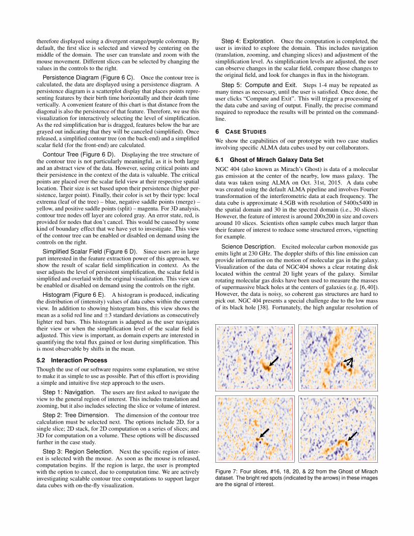
6.1 Ghost of Mirach Galaxy Data SetNGC 404 (also known as Mirach’s Ghost) is data of a moleculargas emission at the center of the nearby, low mass galaxy. Thedata was taken using ALMA on Oct. 31st, 2015. A data cubewas created using the default ALMA pipeline and involves Fouriertransformation of the interferometric data at each frequency. Thedata cube is approximate 4.5GB with resolution of 5400x5400 inthe spatial domain and 30 in the spectral domain (i.e., 30 slices).However, the feature of interest is around 200x200 in size and coversaround 10 slices. Scientists often sample cubes much larger thantheir feature of interest to reduce some structured errors, vignettingfor example.

Science Description. Excited molecular carbon monoxide gasemits light at 230 GHz. The doppler shifts of this line emission canprovide information on the motion of molecular gas in the galaxy.Visualization of the data of NGC404 shows a clear rotating disklocated within the central 20 light years of the galaxy. Similarrotating molecular gas disks have been used to measure the massesof supermassive black holes at the centers of galaxies (e.g. [6, 40]).However, the data is noisy, so coherent gas structures are hard topick out. NGC 404 presents a special challenge due to the low massof its black hole [38]. Fortunately, the high angular resolution of

Figure 7: Four slices, #16, 18, 20, & 22 from the Ghost of Mirachdataset. The bright red spots (indicated by the arrows) in these imagesare the signal of interest.

Figure 8: Result of simplifying using the 3D contour tree on the Ghost of Mirach dataset was worse than expect due to topological pants (tubesconnecting through slices). Top left: Visualization of the 3D contour tree on slice 22. Top right: Simplification of slice 16. Bottom: Simplification ofslices 18, 20, & 22, respectively. The persistent simplification level was 0.00128.

ALMA provides the highest sensitivity to measuring the black holemass.

We can see an example of 4 spectral slices of the dataset inFigure 7. In these 4 slices, the bright red spots represents the signal,while most of the remaining patterns represent noise.

Varying Simplification Levels. Figure 1 shows an exampleof performing simplification on a single 2D spectra (i.e., a singleslice along the frequency axis). The noisy structure is captured bythe 2D contour tree as many low persistence features (lower left).Increasing the level of simplification removes much of this noise(lower middle). However, selecting a simplification level that is tooaggressive may result in loss of signal (lower right).

3D Contour Trees. Since the spectral data are treated as cubes,our collaborators were interested in the structures that would befound using 3D contour trees. The result of capturing the 3D contourtree, shown in Figure 8, was both a surprise and a disappointment.Although many critical points were found, the data suffered fromwhat we describe as topological pants. A topological pair of pantsis a sphere with three disjoint closed discs removed [7]. Essentially,the 3D contours of noisy features form a complex interconnect tubesthrough the volume that are not physically meaningful. This in-terfered with the kind of features that a contour tree can identify.The root cause of this is that each of the spectra are processed inde-pendently, and thus, there is no correlation between noise patternsacross consecutive slices. Simplifying these temporal noise patternsas a whole is not physically meaningful, and they interfere with truefeatures in the data.

2D Contour Tree Stacks. On the other hand, the processingof 2D contour trees was highly successful. However, the domainscientists still needed the ability to process 3D cubes. The obvi-ous solution was to use a series of 2D contour trees to control thesimplification. Figure 10 shows the result of simplifying a stack ofspectra. This example uses a similar level of simplification to the 3Dcontour tree example in Figure 8. In our implementation, level of

Figure 9: Moment 0 analysis of Ghost of Mirach dataset betweenslices 14 and 24 (the range of the signal) using a stack of 2D contourtrees. Top: Visualization of moment 0 for original data. Bottom:Moment 0 results using data with simplification level of 0.0020.

Figure 10: Result of simplifying the Ghost of Mirach dataset using a stack of images with 2D contour trees. Top left: Visualization of the 2D contourtree on slice 22. Top right: Simplification of slice 16. Bottom: Simplification of slices 18, 20, & 22, respectively. The persistent simplification levelwas 0.00138. The simplification level was good for all except slice 20 where a more aggressive level of simplification was called for.

Figure 11: Visualizations of selected slices from the range 100 to 200 of the CMZ data. Top: Slices 100, 120, 140, 160, and 180 beforesimplification, respectively. Bottom: Slices 100, 120, 140, 160, and 180 after simplification, respectively. The simplification level used was 3.45.

simplification is shared between all slices. This works well for slices16, 18, and 22 (top right, bottom left, and bottom right, respectively).However, the level of simplification was not aggressive enough forslice 20 (bottom middle). At this point the user could either selecta more aggressive simplification, or they could choose to simplifyslice 20 separately from the others.

Moment 0 Analysis. Astrophysicists often use what is knownas moment analysis to reduce the 3D spectrum to 2D images. Mo-ment 0, 1, and 2 measure the mass of gas, the direction of gasmovement, and the temperature of gas, respectively. They are allintegrals across the spectra. To demonstrate the noise reducingpower of our approach, we show the result of moment 0 analysis inFigure 9 on the 2D stack simplification from Figure 10. Moment 0is calculated as m0 =

∫Iv, where I is the intensity for a given spectra

v. By removing the noise from each of the layers, the resultingmoment map is significantly less noisy making the signal itself veryapparent. Our collaborator also found the dim feature pointed toby the arrow very interesting. He and his collaborators have beenactively debating whether this structure is signal or a data processing

artifact. Nevertheless, our approach retained it as signal, and weare excited to see how our results generate further conversationsregarding the data.

6.2 CMZ Data SetThe CMZ data are a 13CO 2-1 image of the Central Molecular Zone(CMZ) of the galaxy (data are published in [24]). The data cubeis approximate 500MB with resolution of 1150x200 in the spatialdomain and 500 in the spectral domain (i.e., 500 slices). We look at100 slices of a region with resolution about 300x200.

Science Description. The cube shows the low-density molec-ular gas in the Galaxy’s center, with higher intensities generallyindicating that there is more gas moving at a particular velocityalong each line of sight. It contains highly turbulent gas with proper-ties that are very different than the rest of the Galaxy. The domainscientists use these data to measure the structure of the interstellarmedium, which is important for determining how stars are formedand how galaxies evolve. Because the gas they are seeing is in dif-fuse clouds that do not have well-defined edges, signal identification

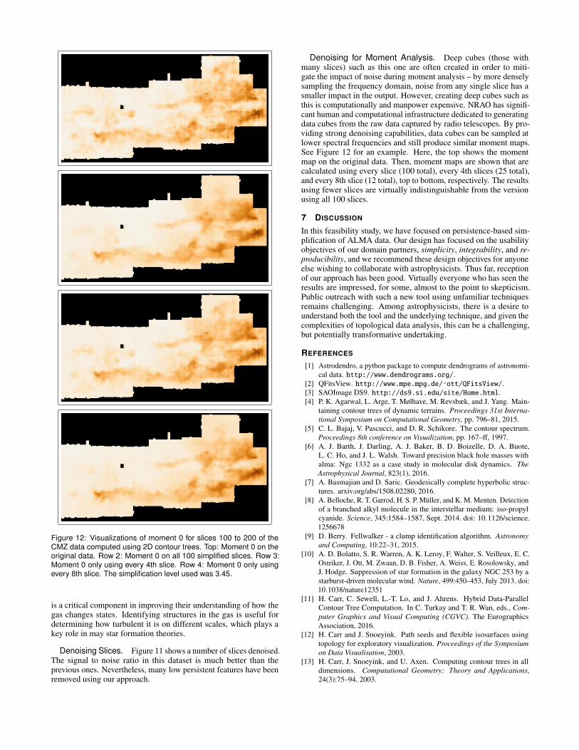
Figure 12: Visualizations of moment 0 for slices 100 to 200 of theCMZ data computed using 2D contour trees. Top: Moment 0 on theoriginal data. Row 2: Moment 0 on all 100 simplified slices. Row 3:Moment 0 only using every 4th slice. Row 4: Moment 0 only usingevery 8th slice. The simplification level used was 3.45.

is a critical component in improving their understanding of how thegas changes states. Identifying structures in the gas is useful fordetermining how turbulent it is on different scales, which plays akey role in may star formation theories.

Denoising Slices. Figure 11 shows a number of slices denoised.The signal to noise ratio in this dataset is much better than theprevious ones. Nevertheless, many low persistent features have beenremoved using our approach.

Denoising for Moment Analysis. Deep cubes (those withmany slices) such as this one are often created in order to miti-gate the impact of noise during moment analysis – by more denselysampling the frequency domain, noise from any single slice has asmaller impact in the output. However, creating deep cubes such asthis is computationally and manpower expensive. NRAO has signifi-cant human and computational infrastructure dedicated to generatingdata cubes from the raw data captured by radio telescopes. By pro-viding strong denoising capabilities, data cubes can be sampled atlower spectral frequencies and still produce similar moment maps.See Figure 12 for an example. Here, the top shows the momentmap on the original data. Then, moment maps are shown that arecalculated using every slice (100 total), every 4th slices (25 total),and every 8th slice (12 total), top to bottom, respectively. The resultsusing fewer slices are virtually indistinguishable from the versionusing all 100 slices.

7 DISCUSSION

In this feasibility study, we have focused on persistence-based sim-plification of ALMA data. Our design has focused on the usabilityobjectives of our domain partners, simplicity, integrability, and re-producibility, and we recommend these design objectives for anyoneelse wishing to collaborate with astrophysicists. Thus far, receptionof our approach has been good. Virtually everyone who has seen theresults are impressed, for some, almost to the point to skepticism.Public outreach with such a new tool using unfamiliar techniquesremains challenging. Among astrophysicists, there is a desire tounderstand both the tool and the underlying technique, and given thecomplexities of topological data analysis, this can be a challenging,but potentially transformative undertaking.

REFERENCES

[1] Astrodendro, a python package to compute dendrograms of astronomi-cal data. http://www.dendrograms.org/.

[2] QFitsView. http://www.mpe.mpg.de/˜ott/QFitsView/.[3] SAOImage DS9. http://ds9.si.edu/site/Home.html.[4] P. K. Agarwal, L. Arge, T. Mølhave, M. Revsbæk, and J. Yang. Main-

taining contour trees of dynamic terrains. Proceedings 31st Interna-tional Symposium on Computational Geometry, pp. 796–81, 2015.

[5] C. L. Bajaj, V. Pascucci, and D. R. Schikore. The contour spectrum.Proceedings 8th conference on Visualization, pp. 167–ff, 1997.

[6] A. J. Barth, J. Darling, A. J. Baker, B. D. Boizelle, D. A. Buote,L. C. Ho, and J. L. Walsh. Toward precision black hole masses withalma: Ngc 1332 as a case study in molecular disk dynamics. TheAstrophysical Journal, 823(1), 2016.

[7] A. Basmajian and D. Saric. Geodesically complete hyperbolic struc-tures. arxiv.org/abs/1508.02280, 2016.

[8] A. Belloche, R. T. Garrod, H. S. P. Muller, and K. M. Menten. Detectionof a branched alkyl molecule in the interstellar medium: iso-propylcyanide. Science, 345:1584–1587, Sept. 2014. doi: 10.1126/science.1256678

[9] D. Berry. Fellwalker - a clump identification algorithm. Astronomyand Computing, 10:22–31, 2015.

[10] A. D. Bolatto, S. R. Warren, A. K. Leroy, F. Walter, S. Veilleux, E. C.Ostriker, J. Ott, M. Zwaan, D. B. Fisher, A. Weiss, E. Rosolowsky, andJ. Hodge. Suppression of star formation in the galaxy NGC 253 by astarburst-driven molecular wind. Nature, 499:450–453, July 2013. doi:10.1038/nature12351

[11] H. Carr, C. Sewell, L.-T. Lo, and J. Ahrens. Hybrid Data-ParallelContour Tree Computation. In C. Turkay and T. R. Wan, eds., Com-puter Graphics and Visual Computing (CGVC). The EurographicsAssociation, 2016.

[12] H. Carr and J. Snoeyink. Path seeds and flexible isosurfaces usingtopology for exploratory visualization. Proceedings of the Symposiumon Data Visualisation, 2003.

[13] H. Carr, J. Snoeyink, and U. Axen. Computing contour trees in alldimensions. Computational Geometry: Theory and Applications,24(3):75–94, 2003.

[14] H. Carr, J. Snoeyink, and M. van de Panne. Simplifying flexibleisosurfaces using local geometric measures. Proceedings 15th IEEEVisualization, pp. 497–504, 2004.

[15] H. Carr, J. Snoeyink, and M. van de Panne. Flexible isosurfaces: Sim-plifying and displaying scalar topology using the contour tree. Compu-tational Geometry: Theory and Applications, 43(1):42–58, 2010.

[16] H. Carr, G. Weber, C. Sewell, and J. Ahrens. Parallel peak pruning forscalable smp contour tree computation. In IEEE Symposium on LargeData Analysis and Visualization, 2016.

[17] Y.-J. Chiang, T. Lenz, X. Lu, and G. Rote. Simple and optimal output-sensitive construction of contour trees using monotone paths. Compu-tational Geometry, 30(2):165 – 195, 2005.

[18] D. Cohen-Steiner, H. Edelsbrunner, and J. Harer. Stability of persis-tence diagrams. Discrete and Computational Geometry, 37(1):103–120,2007.

[19] D. Cohen-Steiner, H. Edelsbrunner, and J. Harer. Extending persistenceusing poincare and lefschetz duality. Foundations of ComputationalMathematics, 9(1):79–103, 2009.

[20] D. Colombo, E. Rosolowsky, A. Ginsburg, A. Duarte-Cabral, andA. Hughes. Graph-based interpretation of the molecular interstellarmedium segmentation. Monthly Notices of the Royal AstronomicalSociety, 454(2):2067–2091, 2015.

[21] C. De Breuck, R. J. Williams, M. Swinbank, P. Caselli, K. Coppin,T. A. Davis, R. Maiolino, T. Nagao, I. Smail, F. Walter, A. Weiss, andM. A. Zwaan. ALMA resolves turbulent, rotating [CII] emission in ayoung starburst galaxy at z = 4.8. Astronomy & Astrophysics, 565:A59,May 2014. doi: 10.1051/0004-6361/201323331

[22] H. Edelsbrunner, D. Letscher, and A. J. Zomorodian. Topologicalpersistence and simplification. Discrete and Computational Geometry,28:511–533, 2002.

[23] H. Edelsbrunner, D. Morozov, and V. Pascucci. Persistence-sensitivesimplification of functions on 2-manifolds. Proceedings of the AnnualACM Symposium on Computational Geometry, pp. 127–134, 2006.

[24] A. Ginsburg, C. Henkel, Y. Ao, D. Riquelme, J. Kauffmann, T. Pillai,E. A. Mills, M. A. Requena-Torres, K. Immer, L. Testi, et al. Dense gasin the galactic central molecular zone is warm and heated by turbulence.Astronomy & Astrophysics, 586:A50, 2016.

[25] A. A. Goodman, E. W. Rosolowsky, M. A. Borkin, J. B. Foster,M. Halle, J. Kauffmann, and J. E. Pineda. A role for self-gravityat multiple length scales in the process of star formation. Nature,457(7225):63–66, 2009.

[26] C. Gueunet, P. Fortin, J. Jomier, and J. Tierny. Contour forests: Fastmulti-threaded augmented contour trees. In IEEE Symposium on LargeData Analysis and Visualization, 2016.

[27] P. J. Hancock, T. Murphy, B. M. Gaensler, A. Hopkins, and J. R. Curran.Compact continuum source-finding for next generation radio surveys.Monthly Notices of the Royal Astronomical Society, 422(2), 2012.

[28] A. M. Hopkins, M. T. Whiting, N. Seymour, K. E. Chow, R. P. Norris,L. Bonavera, R. Breton, D. Carbone, C. Ferrari, T. M. O. Franzen,H. Garsden, J. Gonzalez-Nuevo, C. A. Hales, P. J. Hancock, G. Heald,D. Herranz, M. Huynh, R. J. Jurek, M. Lopez-Caniego, M. Mas-sardi, N. Mohan, S. Molinari, E. Orru, R. Paladino, M. Pestalozzi,R. Pizzo, D. Rafferty, H. J. A. Rottgering, L. Rudnick, A. Schisano,E.and Shulevski, J. Swinbank, R. Taylor, and A. J. van der Horst. Theaskap/emu source finding data challenge. Publications of the Astro-nomical Society of Australia, 32, 2015.

[29] K. E. Johnson, A. K. Leroy, R. Indebetouw, C. L. Brogan, B. C. Whit-more, J. Hibbard, K. Sheth, and A. S. Evans. The Physical Conditionsin a Pre-super Star Cluster Molecular Cloud in the Antennae Galaxies.The Astrophysical Journal, 806:35, June 2015. doi: 10.1088/0004-637X/806/1/35

[30] A. K. Leroy, A. D. Bolatto, E. C. Ostriker, E. Rosolowsky, F. Wal-ter, S. R. Warren, J. Donovan Meyer, J. Hodge, D. S. Meier, J. Ott,K. Sandstrom, A. Schruba, S. Veilleux, and M. Zwaan. ALMA Revealsthe Molecular Medium Fueling the Nearest Nuclear Starburst. TheAstrophysical Journal, 801:25, Mar. 2015. doi: 10.1088/0004-637X/801/1/25

[31] H. B. Liu, R. Galvan-Madrid, I. Jimenez-Serra, C. Roman-Zuniga,Q. Zhang, Z. Li, and H.-R. Chen. ALMA Resolves the Spiraling Accre-tion Flow in the Luminous OB Cluster-forming Region G33.92+0.11.

The Astrophysical Journal, 804:37, May 2015. doi: 10.1088/0004-637X/804/1/37

[32] S. Maadasamy, H. Doraiswamy, and V. Natarajan. A hybrid parallelalgorithm for computing and tracking level set topology. In HiPC, pp.1–10. IEEE Computer Society, 2012.

[33] S. McKenna, D. Mazur, J. Agutter, and M. Meyer. Design activityframework for visualization design. IEEE Transactions on Visualiza-tion & Computer Graphics, 20:2191–2200, 2014.

[34] D. S. Meier, F. Walter, A. D. Bolatto, A. K. Leroy, J. Ott,E. Rosolowsky, S. Veilleux, S. R. Warren, A. Weiss, M. A. Zwaan, andL. K. Zschaechner. ALMA Multi-line Imaging of the Nearby StarburstNGC 253. The Astrophysical Journal, 801:63, Mar. 2015. doi: 10.1088/0004-637X/801/1/63

[35] E. Merenyi, J. Taylor, and A. Isella. Mining complex hyperspectralalma cubes for structure with neural machine learning. IEEE Sympo-sium Series on Computational Intelligence (SSCI), 2016.

[36] D. Morozov and G. Weber. Distributed merge trees. In Proceedingsof the 18th ACM SIGPLAN Symposium on Principles and Practice ofParallel Programming, pp. 93–102. New York, NY, USA, 2013.

[37] D. Morozov and G. H. Weber. Distributed Contour Trees, pp. 89–102.Springer International Publishing, Cham, 2014.

[38] D. D. Nguyen, A. C. Seth, M. den Brok, N. Neumayer, M. Cappellari,A. J. Barth, N. Caldwell, B. F. Williams, and B. Binder. Improveddynamical constraints on the mass of the central black hole in ngc 404.The Astrophysical Journal, 836(2), 2017.

[39] P. Oesterling, C. Heine, G. Weber, D. Morozov, and G. Scheuer-mann. Computing and visualizing time-varying merge trees for high-dimensional data. Workshop on Topology-Based Methods in Visual-ization (TopoInVis), May 2015.

[40] K. Onishi, S. Iguchi, T. A. Davis, M. Bureau, M. Cappellari, M. Sarzi,and L. Blitz. Wisdom project - i: Black hole mass measurement usingmolecular gas kinematics in ngc 3665. Accepted to Monthly Notices ofthe Royal Astronomical Society (MNRAS), 2017.

[41] A. Partnership, C. L. Brogan, L. M. Perez, T. R. Hunter, W. R. F.Dent, A. S. Hales, R. Hills, S. Corder, E. B. Fomalont, C. Vlahakis,Y. Asaki, D. Barkats, A. Hirota, J. A. Hodge, C. M. V. Impellizzeri,R. Kneissl, E. Liuzzo, R. Lucas, N. Marcelino, S. Matsushita, K. Nakan-ishi, N. Phillips, A. M. S. Richards, I. Toledo, R. Aladro, D. Broguiere,J. R. Cortes, P. C. Cortes, D. Espada, F. Galarza, D. Garcia-Appadoo,L. Guzman-Ramirez, E. M. Humphreys, T. Jung, S. Kameno, R. A.Laing, S. Leon, G. Marconi, A. Mignano, B. Nikolic, L.-A. Nyman,M. Radiszcz, A. Remijan, J. A. Rodon, T. Sawada, S. Takahashi,R. P. J. Tilanus, B. Vila Vilaro, L. C. Watson, T. Wiklind, E. Akiyama,E. Chapillon, I. de Gregorio-Monsalvo, J. Di Francesco, F. Gueth,A. Kawamura, C.-F. Lee, Q. Nguyen Luong, J. Mangum, V. Pietu,P. Sanhueza, K. Saigo, S. Takakuwa, C. Ubach, T. van Kempen,A. Wootten, A. Castro-Carrizo, H. Francke, J. Gallardo, J. Garcia,S. Gonzalez, T. Hill, T. Kaminski, Y. Kurono, H.-Y. Liu, C. Lopez,F. Morales, K. Plarre, G. Schieven, L. Testi, L. Videla, E. Villard,P. Andreani, J. E. Hibbard, and K. Tatematsu. First Results from HighAngular Resolution ALMA Observations Toward the HL Tau Region.ArXiv e-prints, Mar. 2015.

[42] A. Partnership, C. Vlahakis, T. R. Hunter, J. A. Hodge, L. M. Perez,P. Andreani, C. L. Brogan, P. Cox, S. Martin, M. Zwaan, S. Mat-sushita, W. R. F. Dent, C. M. V. Impellizzeri, E. B. Fomalont, Y. Asaki,D. Barkats, R. E. Hills, A. Hirota, R. Kneissl, E. Liuzzo, R. Lu-cas, N. Marcelino, K. Nakanishi, N. Phillips, A. M. S. Richards,I. Toledo, R. Aladro, D. Broguiere, J. R. Cortes, P. C. Cortes, D. Espada,F. Galarza, D. Garcia-Appadoo, L. Guzman-Ramirez, A. S. Hales, E. M.Humphreys, T. Jung, S. Kameno, R. A. Laing, S. Leon, G. Marconi,A. Mignano, B. Nikolic, L.-A. Nyman, M. Radiszcz, A. Remijan, J. A.Rodon, T. Sawada, S. Takahashi, R. P. J. Tilanus, B. Vila Vilaro, L. C.Watson, T. Wiklind, Y. Ao, J. Di Francesco, B. Hatsukade, E. Hatz-iminaoglou, J. Mangum, Y. Matsuda, E. van Kampen, A. Wootten,I. de Gregorio-Monsalvo, G. Dumas, H. Francke, J. Gallardo, J. Gar-cia, S. Gonzalez, T. Hill, D. Iono, T. Kaminski, A. Karim, M. Krips,Y. Kurono, C. Lonsdale, C. Lopez, F. Morales, K. Plarre, L. Videla,E. Villard, J. E. Hibbard, and K. Tatematsu. ALMA Long BaselineObservations of the Strongly Lensed Submillimeter Galaxy HATLASJ090311.6+003906 at z=3.042. ArXiv e-prints, Mar. 2015.

[43] V. Pascucci, K. Cole-McLaughlin, and G. Scorzelli. Multi-resolutioncomputation and presentation of contour trees. Technical Report UCRL-PROC-208680, Lawrence Livermore National Laboratory, 2005.

[44] V. Pascucci, G. Scorzelli, P.-T. Bremer, and A. Mascarenhas. Robuston-line computation of Reeb graphs: Simplicity and speed. ACMTransactions on Graphics, 26(3):58.1–58.9, 2007.

[45] N. Peretto, G. A. Fuller, A. Duarte-Cabral, A. Avison, P. Hennebelle,J. E. Pineda, P. Andre, S. Bontemps, F. Motte, N. Schneider, andS. Molinari. Global collapse of molecular clouds as a formation mecha-nism for the most massive stars. Astronomy & Astrophysics, 555:A112,July 2013. doi: 10.1051/0004-6361/201321318

[46] B. Raichel and C. Seshadhri. A mountaintop view requires minimalsorting: A faster contour tree algorithm. CoRR, abs/1411.2689, 2014.

[47] J. M. Rathborne, S. N. Longmore, J. M. Jackson, J. F. Alves, J. Bally,N. Bastian, Y. Contreras, J. B. Foster, G. Garay, J. M. D. Kruijssen,L. Testi, and A. J. Walsh. A Cluster in the Making: ALMA Reveals theInitial Conditions for High-mass Cluster Formation. The AstrophysicalJournal, 802:125, Apr. 2015. doi: 10.1088/0004-637X/802/2/125

[48] J. M. Rathborne, S. N. Longmore, J. M. Jackson, J. M. D. Kruijssen,J. F. Alves, J. Bally, N. Bastian, Y. Contreras, J. B. Foster, G. Garay,L. Testi, and A. J. Walsh. Turbulence Sets the Initial Conditions for StarFormation in High-pressure Environments. The Astrophysical JournalLetters, 795:L25, Nov. 2014. doi: 10.1088/2041-8205/795/2/L25

[49] P. Rosen, J. Tu, and L. Piegl. A hybrid solution to calculating aug-mented join trees of 2d scalar fields in parallel. In CAD Conferenceand Exhibition (accepted), 2017.

[50] E. Rosolowsky and A. Leroy. Bias-free measurement of giant molecularcloud properties. The Publications of the Astronomical Society of thePacific, 118(842):590–610, 2006.

[51] E. W. Rosolowsky, J. E. Pineda, J. Kauffmann, and A. A. Goodman.Structural analysis of molecular clouds: Dendrograms. The Astrophysi-cal Journal, 679(2):1338–1351, 2008.

[52] D. Schneider, A. Wiebel, H. Carr, M. Hlawitschka, and G. Scheuer-mann. Interactive comparison of scalar fields based on largest contourswith applications to flow visualization. IEEE Transactions on Visual-ization and Computer Graphics, 14(6):1475–1482, 2008.

[53] B.-S. Sohn and C. Bajaj. Time-varying contour topology. IEEE Trans-actions on Visualization and Computer Graphics, 12(1):14–25, 2006.

[54] M. van Kreveld, R. van Oostrum, C. L. Bajaj, V. Pascucci, andD. Schikore. Contour trees and small seed sets for isosurface traversal.Proceedings 19th Annual symposium on Computational geometry, pp.212–220, 1997.

[55] R. Wang, J. Wagg, C. L. Carilli, F. Walter, L. Lentati, X. Fan, D. A.Riechers, F. Bertoldi, D. Narayanan, M. A. Strauss, P. Cox, A. Omont,K. M. Menten, K. K. Knudsen, R. Neri, and L. Jiang. Star Formationand Gas Kinematics of Quasar Host Galaxies at z ˜ 6: New Insightsfrom ALMA. The Astrophysical Journal, 773:44, Aug. 2013. doi: 10.1088/0004-637X/773/1/44

[56] S. Westerlund, C. Harris, and T. Westmeier. Assessing the accuracyof radio astronomy source finding algorithms. Publications of theAstronomical Society of Australia, 29:301–308, 2012.

[57] J. P. Williams, E. J. de Geus, and L. Blitz. Determining structure inmolecular clouds. The Astrophysical Journal, 428(2):693–712, 1994.