Page 1 of 47

Using Bureau of Meteorology multi-week and seasonal forecasts to improve management decisions in Queensland’s vegetable industry

Final Report—June 2021

Project leader – David Carey, Senior Horticulturist, Horticulture and Forestry Science, DAF Qld.

Project team members – Dr Neil White, Principal Scientist, Horticulture and Forestry Science, the Department of Agriculture and Fisheries (DAF); Peter Deuter, Horticultural Consultant, PLD Horticulture, and Dr Debra Hudson, Principal Research Scientist, Bureau of Meteorology (BoM).

David Carey, Neil White and Peter Deuter (referred to in the report as DC, NW, PD) have been responsible for interacting with stakeholders, interpreting the forecasts and assessing their accuracy.

Debra Hudson (DH) has been responsible for providing the ACCESS-S1 experimental forecasts on the R&D Bureau website.

Page 2 of 47

Table of Contents

Summary ............................................................................................................................. 3 Our collaborators ................................................................................................................ 4 Project output highlights and accomplishments. ............................................................. 5 Project impact. .................................................................................................................... 6

External and cross-industry interactions ......................................................................................... 6 Experimental forecast accuracy and usefulness .............................................................. 8

Maximum temperature forecasts..................................................................................................... 8 Minimum temperature forecasts...................................................................................................... 8 Rainfall forecasts……………. .......................................................................................................... 8

Communicating the accuracy of DCAP experimental forecasts. ..................................... 9 DAF#7 Experimental forecasts influencing business managers decisions. ................. 10

Do the forecasts offer the potential for improved management decisions? .................................. 12 Have improved management decisions been identified? ............................................................. 13 Have these decisions positively impacted risk and profitability, and/or product quality and reliability of production and supply?................................................................................................................................13

Does the extra DCAP information help make a better business decisions? ................ 14 DCAP Heatwave Advisories ............................................................................................. 16

Ongoing business manager support and engagement. ................................................................ 17 DCAP Veggie business podcast. .................................................................................................. 19

Building industry confidence in and verifying our DCAP ACCESS S1 LV and GB forecast model grid interpolated data. ............................................................................ 20

Documenting the benefit and impact of the DCAP DAF #7 vegetable industry project. ........................................................................................................................................... 21

Six detailed vegetable industry Case Studies. .............................................................................. 21 Appendix 1. ....................................................................................................................... 22

Assessing the accuracy (skill) of all current DCAP experimental long lead time forecasts. ......... 22 Appendix 2. ....................................................................................................................... 37

Significance testing and forecast assessment .............................................................................. 37 Appendix 3. ....................................................................................................................... 42

Verification of gridded data sets using field measurements ......................................................... 42 Introduction……………………………. ........................................................................................... 42 Results…………………………………….. ...................................................................................... 44 Maximum Temperature………………. .......................................................................................... 44 Minimum Temperature………….................................................................................................... 45 Rainfall…………………………………. .......................................................................................... 46 Discussion……………………………… ......................................................................................... 47

Page 3 of 47

Summary ACCESS-S1 experimental forecasts commenced in Jan 2018, for the Lockyer Valley (LV) and Granite Belt (GB) regions, in a specific format for the DAF#7 DCAP project. The project team have to-date developed and delivered 20 detailed bi-monthly experimental forecasts for our collaborating business managers in the Lockyer Valley and 17 for the Granite Belt. The team has also delivered 15 experimental forecasts for the Bowen production region. There are fewer forecasts for this region as our collaborators do not farm or source product from this region over summer. The DCAP#7 project was the first project to make use of the new R&D website tool for displaying ACCESS-S experimental forecast products for stakeholders in R&D projects. The DCAP#7 project team were the first "testers" and their observations helped resolve issues Forecast data from the BoM experimental website have been converted by project team members into an easily readable format for growers and Qld based national supply chain business managers in the two regions, and delivered to them on a bi-monthly basis. In addition, we have also delivered bi-monthly DCAP Experimental Forecasts to two Lockyer Valley based nationally significant vegetable production and marketing businesses that produce green beans and sweet corn in the Bowen winter growing season and supply to the national supermarket chains every day of the year. The DCAP funded BoM R&D experimental product delivers daily experimental forecasts from ACCESS-S to our R&D site, with some gaps due to occasional technical issues associated with developing a new experimental forecast system. This project has led to increased insight into the potential applications of multi-week and seasonal forecasts by the horticulture sector. In particular, it has become clear that vegetable growers, business managers and supply chain managers collaborating in this project are making a considerable number of weather-related management decisions (e.g. start dates for the planting season; variety to plant; irrigation management), almost on a daily basis, for a range of timescales into the future (from minutes to seasons). In addition, they usually grow multiple crops per year and often have farms in multiple locations across Queensland. There is huge potential for useful forecasts over-and-above what are currently available operationally.

DCAP Heatwave advisories commenced in November 2018 for the Lockyer Valley and Granite Belt forecast region. The Bureau's Heatwave Service was launched in 2014. The Heatwave service was introduced as a human health initiative to warn the Australian public of extreme temperature events. Although not designed with agriculture in mind, it is a publicly available product. Feedback from the DCAP project shows that it has considerable value for the agriculture sector.

This specific information product was developed and delivered as soon as we became aware that the majority (>90%) of our collaborating business managers in both the LV & GB were unaware of this public Heatwave forecast information, available on the BoM web site since (2014). Emailed timely DCAP heatwave advisories with links to the BoM web site were embraced by our collaborators and used very effectively to make better management decisions – improving crop yield, quality and income (refer to anecdotes). We issued 17 Heatwave advisories over the 3 summers of this project. Our project team has from project initiation, worked very closely with BoM R&D staff through regular webinar, email and phone discussions. We have also instigated two, one-day meetings at BoM’s head office in Melbourne since project inception to develop, refine and modify the format and information displayed on BoM’s DCAP experimental forecast website. This one on one personal interaction, combined with our data analysis and feedback has been very beneficial for all. BoM Researchers, the Agriculture team and BoM’s Horticultural Sector Lead, now have a greatly improved understanding of the Queensland vegetable industries’ forecast needs, as well as the impact and potential costs of extreme weather

Page 4 of 47

conditions in Queensland’s vegetable production regions. This high level impact was officially acknowledged in June 2021 feedback from BoM managers (see BoM Case Study). One of the most valuable outcomes of this project, from the Bureau's perspective, has been insight into the utility and value of seasonal forecasts for the horticulture sector. This type of feedback helps the Bureau understand the customer base and identify priorities for future R&D and the transitioning of research into a service. Promotion of operational BoM products and services to grower and supply chain business collaborators, in particular the operational seasonal climate outlooks and the Heatwave Service, has resulted in significantly increased awareness of these services, and has positively influenced BoM decision-making.

The Project Team have also gained a better appreciation of the technical aspects of producing an experimental forecast and converting this to an Operational Product. This close interaction and detailed communication has influenced BoM’s research and operational forecast products, enhancing and informing their forecast display, and empowering their usefulness to Queensland and Australian agricultural producers. The DAF#7 team have educated and enhanced the knowledge and understanding of our Queensland business collaborators over the past 36 months. Supply chain and farm business managers now have a much better understanding of BoM’s systems and forecast methods, as well as a better appreciation of the underlying climate variability and forecasting terminology and methodology. All of our Lockyer Valley and Granite Belt collaborators are still (after 36 months) enthusiastic about the relevance, quality and usefulness of this DAF#7 vegetable project work, especially the long lead time maximum temperature forecasts. Key Queensland supply chain and vegetable production business managers actively use the DCAP DAF#7 experimental forecast information in combination with their improved understanding of BoM opertional forecasts and methodology to make “better management decisions”. The positive $ impact of just some of these better management decisions is detailed in the Case Study 2, developed by the Project team, based on written and SMS information from just 16 of the 48 businesses with whom we have engaged.

Our collaborators The DAF#7 team have been actively engaging with vegetable growing businesses in the Lockyer Valley and Granite Belt regions as well as with nationally significant supply chain managers. Many of our vegetable business collaborators have production systems in multiple locations across Queensland and in some cases also have directly owned interstate production farms and/or contract growers in other states and locations. Several of the larger production operations we collaborate with are vertically integrated. They own and manage large scale packhouses, packing and distribution centres in Queensland and interstate. These businesses supply fresh and prepacked vegetables to the large supermarket chains throughout the East Coast of Australia. These larger production businesses have year round supply contracts that they are bound to fulfill; they are significant local and state employers and very important to the regional economies in which they operate. Our collaborating supply chain business managers service the local and interstate retail supermarkets, specialist fruit and vegetable businesses as well as processors who supply the local and national fast food sector (e.g. McDonalds®, Subway®, KFC® etc). Fresh vegetables and value added product are also exported to meet international orders. Some of these supply co-ordination businesses operate Australia wide and are recognised retail brands (e.g. One Harvest & Perfection Fresh) that you would have seen on your local supermarket shelves. Several of our other collaborating supply chain managers service the food sector, supplying processed or semi-processed fresh vegetables to the restaurant, catering and fast food industry (e.g. Lite n’ Easy, You Foodz, Subway, McDonald’s)

Page 5 of 47

Project output highlights and accomplishments Since January 2018 when we began using our dedicated ACCESS-S1 based regional Lockyer Valley and Granite Belt experimental DCAP forecast model to engage with our collaborators we have:-

• Worked closely with BoM R&D staff in developing our DCAP vegetable region tailored ACCESS-S forecast climate model.

• Organised and held 14 “face to face” DCAP Experimental Forecast Forums (each is a 2 to 2.5 hour long informative, educational presentation, including an interactive discussion session).

• Developed and distributed 42 bi-monthly experimental forecasts for our collaborating business managers in the Lockyer Valley, Granite Belt and 15 for the Bowen region.

• Developed and issued 17 DCAP Heatwave Advisory warnings to collaborating businesses (during spring and summer).

• Held over 80 one on one DCAP related discussions with individual project collaborators.

• Organised dedicated meetings with DCAP collaborators to discuss and document what management decisions they would change if they had access to a reliable long lead time forecast.

• Contributed 7 media pieces to DCAP eNews, presented on-line to the Birchip Cropping Group, organised a DCAP Podcast, promoted our DCAP work in the Granite Belt Advertiser magazine and had a separate LV grower article in the Gatton Star.

• Researched and written a Journal article, which has been sumitted and is being assessed and reviewed by the editor of the Journal of Applied Meteorology and Climatology. The manuscript "Documenting the financial impact of extreme summer heat on Lockyer Valley Capsicum production”, documents the “real life” loss of income caused by fruit sunburn on a commercial Lockyer Valley farm.

• We have conducted 14 surveys of collaborating businesses, in both the Granite Belt and Lockyer Valley region, to measure and monitor the impact of information presented by the DAF #7 project team, and gauge their ongoing appetite for, interest in, and opinion of this DCAP experimental forecast work.

• Assessed and statistically analysed the accuracy of every DCAP experimental forecast (41 in total) distributed to our poject collaborators since since July 2018.

• Presented and discussed our DCAP experimental forecast accuracy with our business collaborators at regional face to face experimental forecast forums.

• Documented the monetary benefit (extra income) of better management decisions reported to us by our business collaborators (Marketing & supply chain Case Study).

• Documented the significant high level impact the DAF#7 poject team has had by raising BoM’s awareness and responsiveness to the unique forecast needs of Queensland vegetable growers and the entire horticulture industry (BoM Case Study).

• Investigated, measured and documented how and why extreme temperatures and low humidity reduce sweet corn yield by causing kernel blanking in summer plantings in the Lockyer Valley. This “field based information analysis and understanding will help industry minimise this issue in coming seasons. These better informed decisions will make them $ (Sweet corn industry case study).

• Documented and detailed the impact of Heatwaves reported by our project collaborators (Heatwave Case Study)

• Detailed, measured and analysed the actual income loss of a commercial Lockyer Valley capsicum business during extreme summer heat (Capsicum Case Study)

Page 6 of 47

• Demonstrated and documented the “real life” financial value of this DCAP investment. The investment of $264K in project funding and 3 years of hard work by the Project Team has resulted in a minimum of $688K of extra income from better decisions – as reported voluntarily by 16 of our collaborating business managers (Collaboratore cost benefit Case Study).

Project impact We have always been very aware that project funding would end in June 2021 and have thought long and hard about what useful (publicly available) forecasting tools we can leave our collaborators with when our project work ends. We have had detailed conversations with the DCAP Program Manager and BoM R&D staff about future operational products that will be made available to the Horticultural industry at the end of DCAP2 (see BoM Case Study). The horticultural industry is clammering for better quality, publicly available useable long-leadtime forecast information. The project team has throughout the entire project’s life set out to educate, expand and improve our collaborators understanding of publicly available forecasts. Collaborating business managers in the LV and GB state that they now (June 2021) have a better understanding of BoM forecast terminology and improved awareness and adoption of BoM’s publicaly available forecast tools, e.g., MetEye, Heatwave service & Outlook website. The project team has championed and demonstrated these tools to our collaborators who now regularly access, understand and actively use this information as part of their forward planning (see Heatwave Case Study).

External and cross-industry interactions

• David Carey presented an overview of the project’s results to a Farmers for Climate Action local meeting held in April 2019 in Stanthorpe (180 attendees).

• David Carey presented (via webinar) to the Victorian based Birchip Seasonal Climate forecasting Community of Practice group in April 2019. This presentation resulted in requests for follow up information from both BoM and CSIRO staff who attended the webinar.

• Peter Deuter has engaged with the DCAP Insurance project staff (USQ) on multiple occasions and provided them with specific horticultural crop information, feedback, crop specific critical temperature information and yield data to assist their project work on parametric insurance products.

• DAF#7 team members have worked closely with two major sweet corn supply chain businesses to document and measure the impact of heatwave conditions on crop yield in the Lockyer Valley in the last two summers. This detailed data collection and analysis has improved the business mangers understanding of the relationship between summer crop yield loss, high temperature, low humidity and irrigation techniques. This industry focussed work will contribute to a DAF #7 DCAP Case Study that forms part of this final report.

• The DAF#7 team facilitated the production of a DAF Turf ‘n’ Surf Podcast in which a Lockyer Valley production manager highlights the impact of climate drivers on business profitability.

• In August 2020 the DAF media team highlighted DAF #7 Project work and overarching DCAP work in a local Granite Belt magazine.

• In September the Mareeba District Fruit and Vegetable Growers Association was briefed on, and provided with information about our current DAF#7 project work. We were approached by them with a request for information about our current

Page 7 of 47

experimental forecast work with vegetable growers in the Lockyer Valley and Granite Belt.

• During our last 3 “face to face” experimental forecast forums we have accessed and utilised Rainfall and Pasture Growth Posters from DES Grazing Land Systems (DCAP ‘Inside Edge’ project), highlighting and handing out Australia’s Variable Rainfall posters, at our regional meetings. Some of these posters now adorn the walls of our LV and GB business managers offices and one set is on the classroom wall at a local school. (Web link; https://www.longpaddock.qld.gov.au/rainfall-poster/map-app/)

Page 8 of 47

Experimental forecast accuracy and usefulness Is there sufficient skill (accuracy) for these forecasts to be useful? We have “ground-truthed” all 42 long lead time forecasts that have been issued, by comparing forecasts with actual BoM data (rainfall, minimum and maximum temperature) for the Lockyer Valley and Granite Belt regions. This analysis of accuracy is regularly presented to, and discussed with our collaborating business managers as part of our “face to face” local forecast meetings.

Maximum temperature forecasts

To date maximum temperature forecasts have been the most accurate and useful. The 1, 2 and 3 month lead time maximum temperature Lockyer Valley forecasts to date were 74%, 71% and 74% Consistent and accurate respectively. The 1, 2 and 3 month lead time Granite Belt maximum temperature forecasts were 67%, 69% and 60% Consistent and accurate, respectively. The 3 month long lead time maximum temperature foreast based on the 1st available forecast of the month has been 72% Consistent and accurate for the Lockyer Valley region and 62 % Consistent for the Granite Belt region. Maximum temperature forecast accuracy in both regions at all lead times has consistently been useful to our collaborating business managers.

Minimum temperature forecasts

Minimum temperature forecast accuracy for the Lockyer Valley at all lead times, 1, 2 and 3 months, was 37%, 33% and 38% Consistent respectively. The accuracy of the Granite Belt minimums at all lead times, 1, 2 and 3 months, has been 49%, 45% and 44% Consistent respectively. The 3 month long lead time minimum forecast based on the 1st available forecast of the month has been 31% Consistent for the Lockyer Valley region and 38% Consistent for the Granite Belt region. The minimum temperature long lead time forecast in both regions has not been useful to-date.

Rainfall forecasts

Rainfall forecast accuracy at 1,2,and 3 months lead time for the Lockyer Valley has been 63%, 45% and 54% Consistent respectively based on the 42 available forecasts the DCAP team has produced to-date. Rainfall forecast accuracy at 1, 2, and 3 months for the Granite Belt forecast region has been 68%, 55% and 49% Consistent, respectively based on the 42 experimental DCAP forecasts. The 1 month lead time rainfall forecast in both the Lockyer Valley and Granite Belt has been useful to-date while the 2 and 3 month long lead time forecasts in both regions has not been useful to-date.

Page 9 of 47

The three month long lead time experimental rainfall forecasts for the Lockyer Valley and Granite Belt based on the 1st available forecast of the month show a forecast accuracy of 37% and 34% Consistent, respectively. The 3 month long lead time rainfall forecast based on the 1st available forecast has not been useful to-date.

Communicating the accuracy of DCAP experimental forecasts Every two months an experimental forecast for each region is sent to all our business collaborators, and contains a detailed review of the previous forecast period’s accuracy (max, min & rainfall), allowing our project collaborators to assess the skill and usefullness of the experimental forecast information. During our face to face, start and end of season meetings the project team has presented a full review of the accuracy of all experimental forecasts (min, max and rainfall) to our collaborating business managers. This ensures that all collaborating supply chain and vegetable business managers have the opportunity to assess the overall accuracy of maximinum, minimum and rainfall forecasts, allowing them to develop a well informed understanding and opinion of the skill and usefullness of the DCAP Experimental Forecasts. A full analysis of the accuracy and skill of all DCAP Experimental Forecasts from January 2018 to-date in both regions has been completed for this June 2021 Final Report. Appendix 1 (page 88) provides details of the experimental forecast analysis, which outlines the accuracy of all forecasts for both experimental forecast regions. Our ongoing analysis shows that the accuracy and skill of each forecast paramater varies with location and month. The maximum temperature forecasts for both the Lockyer Valley and Granite Belt has proven to be the most accurate and therefore a useful forecast. The overall accuracy of the 1, 2 and 3 month lead time maximum temperature forecast in the Lockyer Valley has been 74%, 71% and 74%, Consistent and accurate respectively. The Granite Belt maximum temperature experimental forecast has been Consistent and accurate 67%, 69% and 60 % of the time for the 1, 2 and 3 month lead time, respectively. There is sufficient accuracy in the long lead time maximum temperature forecasts to be useful to business managers in both regions. The long lead time 1 month rainfall forecast has proven moderately useful in both experimental forecast regions while the skill and accuracy of the minimum temperature forecast has been poor in both production regions. Long lead time maximum temperature forecasting has been the focus of this project (as per the original project proposal), however growers and supply chain managers continue to show interest in long lead time minimum temperature and rainfall forecasts, so we have continued to provide and “ground truth” these additional forecasts, even when the accuracy to-date has not been sufficient for these additional forecasts to be considered useful.

Page 10 of 47

DAF#7 Experimental forecasts influencing business managers decisions Anonymous survey responses gathered at our recent September (Granite Belt) and November (Lockyer Valley) 2020 face to face forecast forums, demonstrate that our collaborating vegetable businesses and supply chain managers consider the DCAP experimental forecast information helps them make better (more informed) management decisions. Producers and supply chain managers have been influenced by the bi-monthly DCAP experimental forecast information.

Figure 1. Granite Belt (top) and Lockyer Valley business managers consider and use the DCAP Experimental Forecasts to make improved management decisions (as at June 2021).

All of our Lockyer Valley and Granite Belt vegetable and supply chain business collaborators remain engaged and enthusiastic about the relevance, quality and usefulness of this DAF#7 vegetable project work, especially the long lead time maximum temperature forecasts. Key Queensland business managers are using the DCAP DAF#7 experimental forecast information in combination with their improved understanding of BoM opertional forecasts and methodology to make “better management decisions”.

Page 11 of 47

Figure 2. Anonymous survey response from collaborating business managers during the June 2021 Lockyer Valley DCAP “start of winter season” experimental forecast forum (40% rated usefulness as high value, 60% as moderate to high).

Example: We have a number of business manager anecdotes included as part of this final report. The whole project concept and work program came from our industry knowledge and belief that an accurate long lead time forecast would allow business managers to make better (more informed decisions). The email below fom a multi-location LV business manager is a good example of the financial benefits that has resulted from these improved decisions. See Case Study section for more examples.

Figure 3. Emailed business feedback demonstrating the financial benefits that have been released through involvement in this DCAP experimental forecasts project work since its inception.

Page 12 of 47

Do the forecasts offer the potential for improved management decisions? Yes. Many of our the collaborating vegetable grower businesses, as well as supply chain managers, have stated and given practical examples of how valuable an accurate long lead time forecast is to their respective operations. A long lead time forecast is a vital management tool, and we have documented real world examples (including the $ impact) of the positive impact on crop yield and farm incomes that have been achieved since our DCAP project team has been communicating experimental forecast information to, and working closely with, our collaborating business partners.

Example: In March this year a Lockyer Valley production manager attended the local start of winter season DCAP meeting where we presented and discussed the 3 month long lead time forecast, below.

Figure 4. Extract from the March 2020 Lockyer Valley DCAP Experimental Forecast for March, April & May 2020. Production manager feedback and improved management decision after reading this forecast appears below.

In 2020, maximum and minimum temperatures for March, April and May were forecast to be above average while the forecast for rainfall was for near or below the mean. On seeing this additional information this production manager reviewed his planting plans and decided not to plant his next scheduled 12 ha of Green Bean crops on the home farm where underground water levels were in decline, and instead moved these plantings to different locations. To give the reader some context, 12 ha of Green Beans would yield around 60,000 Kg or 6,000 boxes of marketable Green Beans with an average market value of $132,000 (6,000 boxes at averge price of $22 a box)

Figure 5. SMS message from production manager the morning after our Lockyer Valley meeting in March 2020.

Page 13 of 47

The additional DCAP experimental forecast information and discussion we provided influenced and assisted this production manager to make (what turned out to be – see below) a better decision, ensuring they had sufficient fresh product to supply and meet retail market orders.

A recent review of the actual rainfall and temperatures that occurred in the Lockyer Valley in March, April and May 2020 shows the long term mean rainfall total 1990-2012 in the Lockyer Valley for these three months is 163.6mm. In 2020 the total rainfall recorded in these three months was only 60 mm. Maximum temperatures in March, April and May 2020 were 3.50C, 1.00C & 1.60C above the long term mean (respectively).

Have improved management decisions been identified?

Yes. Throughout the duration of this project the project team has received numerous documented real life examples of improved management decisions made by supply chain managers and production managers as a result of the DCAP bi-monthly experimental forecast information.

Production managers have:

• changed and finessed planting schedules based on additional DCAP experimental forecasts,

• selected and changed varieties to match forecast conditions, • moved to alternate production locations, • altered both irrigation methods and schedules, • decided to plant only a portion of their normal planting program, or in some cases in

the Granite Belt region – not planted at all due to a lack of forecast rain to replenish dams.

We have documented examples of supply chain managers :-

• changing production supply locations, • reviewing crop selections, • adjusting the size and growing location of production orders, by location and volume • entering into contract growing arrangements with new interstate growers so as to

ensure continuity of supply when the experimental forecast indicated adverse growing conditions in the GB or LV regions.

A detailed list of the financial benefits that have flowed from work for 16 (out of the 48) of our collaborating business managers (who sent us “real life” outcomes) are documented in the attached Cost Benefit analysis Case Study.

Example: A GB based commercial sales agonomist who services many GB vegetable businesses was an active and enthusiastic collaborator in this project. Recent written feedback from him detailed how the bi-monthly forecasts had been very useful to him and his growers. In one instance in the extreme heat of the 2019-20 season DCAP experimental forecast information lead to a better decision by choosing to plant a more heat tollerant cauliflower variety – resulting in a $100 000 benefit to the farm business.

Have these decisions positively impacted risk and profitability, and/or product quality and reliability of production and supply?

Yes. We have documented from the outset of this project, real life examples that demonstrate how the DAF#7 long lead time experimental forecasts, as well as the Heatwave Advisories, combined with our informative pre and post season Experimental Forecast meetings have empowered business managers to make better management decisions.

Page 14 of 47

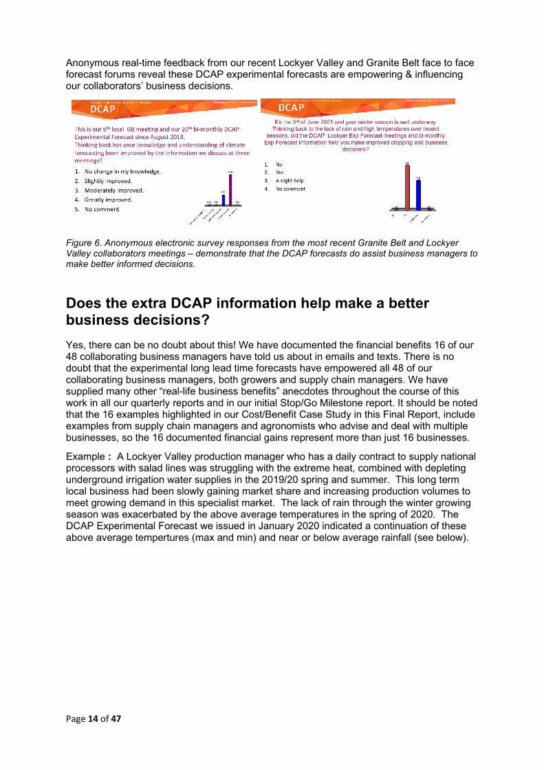
Anonymous real-time feedback from our recent Lockyer Valley and Granite Belt face to face forecast forums reveal these DCAP experimental forecasts are empowering & influencing our collaborators’ business decisions.

Figure 6. Anonymous electronic survey responses from the most recent Granite Belt and Lockyer Valley collaborators meetings – demonstrate that the DCAP forecasts do assist business managers to make better informed decisions.

Does the extra DCAP information help make a better business decisions? Yes, there can be no doubt about this! We have documented the financial benefits 16 of our 48 collaborating business managers have told us about in emails and texts. There is no doubt that the experimental long lead time forecasts have empowered all 48 of our collaborating business managers, both growers and supply chain managers. We have supplied many other “real-life business benefits” anecdotes throughout the course of this work in all our quarterly reports and in our initial Stop/Go Milestone report. It should be noted that the 16 examples highlighted in our Cost/Benefit Case Study in this Final Report, include examples from supply chain managers and agronomists who advise and deal with multiple businesses, so the 16 documented financial gains represent more than just 16 businesses.

Example : A Lockyer Valley production manager who has a daily contract to supply national processors with salad lines was struggling with the extreme heat, combined with depleting underground irrigation water supplies in the 2019/20 spring and summer. This long term local business had been slowly gaining market share and increasing production volumes to meet growing demand in this specialist market. The lack of rain through the winter growing season was exacerbated by the above average temperatures in the spring of 2020. The DCAP Experimental Forecast we issued in January 2020 indicated a continuation of these above average tempertures (max and min) and near or below average rainfall (see below).

Page 15 of 47

Figure 7. January 2020 Lockyer Valley experimental forecast

This additional DCAP Experimental Forecast information prompted this business manager to “take stock and consider their supply position”, which was being negatively impacted by high temperatures and dwindling irrigation water quality and availability. The end result was a decision to purchase another farm in a different location to spread production risk and obtain a more secure irrigation water supply. That decision has turned out to be a very good one, allowing the business to continue to supply salad products and retain their staff while the heat and drought conditions continued in the Lockyer Valley.

Page 16 of 47

DCAP Heatwave Advisories The DCAP project team has raised industry awareness and use of an existing but previously mostly unused BoM operational product.

In the first season (2018) of our local face to face forecast forums with both Lockyer Valley and Granite Belt collaborators, it became apparent that over 70% of these business managers were not aware of BoM’s publicly available and very useful Heatwave Service. The Bureau’s heatwave service has published 7-day heatwave severity maps on the internet since 2014 (Bureau of Meteorology, 2014).

Figure 8. Collaborating business managers were mostly unaware of the BoM Heatwave service until DCAP DAF#7 project staff highlighted it and promoted it usefulness.

In November 2018 we took the initiative to utilise and promote this operational BoM Heatwave Service as one of several additional sources of information to assist our collaborators to make “better management decisions”.

The project team witnessed first hand the value and impact of the DCAP Heatwave Advisories. During the November 2018 LV Exprimental Forecast Forum, we advised the attendees that BoM had that afternoon issued a Heatwave warning that woud impact the LV. Project team members showed and discussed the DCAP Heatwave Advisory we planned to send out. We displayed the BoM Heatwave Service maps and discussed the severity and duration of the approaching heatwave event, which was due to impact the LV within 3 days. Immediately after that meeting several agronomists from one corporate farm formed a huddle in the foyer and decided to delay seeding of that weeks’ Green Bean planting until after the heatwave had dissipated. They also sent SMS messages to all farm managers directing them to put spray irrigation pipes into all Green Bean plantings that were flowering, so that they could overhead irrigate those crops during the heatwave. This type of irrigation reduces flower drop (caused by excessive heat), so increasing potential yield and maximising and sales potential at a time when other suppliers were likely to suffer yield loss, causing a market shortage that would generate higher sale prices.

This initiative has been a resounding success and to-date the project team has developed and issued 17 Heatwave Advisory warnings to collaborating businesses (during spring and summer). The DCAP Heatwave Advisories are emailed directly to all our collaborators, they contain the BoM Heatwave Service maps and a link to BoM’s Heatwave Service.

The project team also includes the detailed 6 day BoM MetEye® forecast for the two BoM weather station locations in the experimental forecast regions, highlighting the expected conditions for collaborating business managers. This forecast format also raised awareness and use of BoM’s MetEye® product. (Web link:http://www.bom.gov.au/australia/meteye/).

Collaborating business managers now actively seek out and use BoM’s Heatwave Service website over the summer season. This awareness and additional knowledge allows them to better prepare for extreme temperature events (heatwaves) that will impact their production location. Collaborating business managers can access the BoM Heatwave Service site to get updates on the day the event is forecast to arrive at their location, the severity of the

Page 17 of 47

event, monitor it’s forecast duration and determine on what day the heatwave is likely to dissipate.

Figure 9. November 2020 DCAP Heatwave Advisory sent to our Lockyer Valley and Granite Belt collaborating business managers.

DCAP Heatwave Advisories (based on the Bureau of Meteorology’s Heatwave Service) have proved to be extremely useful to our collaborating business managers. This extra information has prompted many improved management decisions.

We have previously provided numerous anecdotes from business managers detailing how the information about and awareness of an approaching heatwave has helped them make improved management decisions that have increased business profitability. A number of detailed examples are included in the Heatwave Case Study.

Ongoing business manager support and engagement.

The DCAP Experimental Forecast work and local face to face educational forecast forums have been highly valued.

Collaborating business managers at our two recent regional face to face experimental forecast update meetings have unanimously considered the information presented as being informative and useful.

Figure 10. Collaborating business manager anonymous feedback from our final May 2021 (Granite Belt) and June (Lockyer Valley) 2021 DCAP Forecast Forums.

Page 18 of 47

Industry leaders support the DAF#7 team’s work and values the experimental forecast information

Our collaborators view the DCAP Experimental Forecasts as science based information that they consider when preparing for and making management decisions. The information helps them to make better (more informed) business decisions.

Example email feedback

1. Granite Belt collaborator (emailed) quote. “This is perhaps one of the most worthwhile projects undertaken by a government department in a long time. SURELY HAVING A BETTER UNDERSTANDING OF OUR EVER CHANGING CLIMATE has to be the greatest management tool for a grower that he can use” (from Ray B).

2.

3.

Page 19 of 47

DCAP Veggie business podcast.

One of our Lockyer Valley business collaborators was featured in a DCAP Podcast, click below to hear his thoughts and comments.

LV Veggie grower podcast Rick Sutton

Page 20 of 47

Building industry confidence in and verifying our DCAP ACCESS S1 LV and GB forecast model grid interpolated data. We deployed mobile weather stations within BoM interpolated data 5Km grid cells to check how the interpolated data compared to spot measurements within the chosen grid cells. The stations were deployed on collaborators farms that were on the outer edges of the DCAP GB and LV model grid and the 12 months of daily readings allowed us to compare actual on-farm daily maximums and minimums with those “interpolated” by BoM and used in our regional forecast models. This was done for two reasons; to check the accuracy of BoM’s interpolated data and thereby allow us to demonstrate to our collaborating business managers that the gridded data accurately reflected on-ground reality and local knowledge about differences between farming areas. This was particularly useful in GB where the topography changes are more significant.

This information shared at our face to face meetings also assisted growers understanding of and confidence in BoM’s Outllook and MetEye forecast tools which both use the same interpolated gridded data. The completed analysis of the relationship between the interpolated BoM data calculate for DCAP model grid squares and the actual daily measured temperatures in the grid squares showed the interpolated data to be very close to the measured data. Maximum temperature was slightly more accurate than minimum temperatures but both were realistic. The interpolated data values in the different reference cells reflected the local topography. This was a valuable exercise and enhanced our collaborators knowledge and confidence in the DCAP model and more importantly in BoM’s on-line MetEye and Outlook forecast tools.

For all the details and to read the full analysis please refer to Appendix: 2

21

Documenting the benefit and impact of the DCAP DAF #7 vegetable industry project Six detailed vegetable industry case studies

The following 6 Case Studies explain in detail, and demonstrate the impact of, our small teams work with and focus on the forecast information needs of our collaborating Lockyer Valley and Granite Belt growers and supply chain business managers. We devised and implemented this work with the belief that a better more accurate long lead time forecast would empower our collaborators to make better business decisions.

We also quickly realised that our interaction and discussions with BoM researchers and BoM managers (through our 2 dedicated annual on site full day meetings at BoM’s head office and multiple phone and on-line discussions) greatly improved BoM’s knowledge and understanding of the forecast needs of the vegetable (& horticulture) industry. This project has also “opened BoM managers eyes” to the value of the vegetable industry and how an accurate long lead time forecast can help business managers make better business and crop management decisions.

The Queensland vegetable industry is a major contributor to direct regional employment as well as a driver of local support industries such as transport, machinery sales and repairs, irrigation suppliers, electricians, fabricators and the wider agricultural supply industry. A number of our business collaborators operate year round, growing and packing across multiple sites, and are significant local employers (several with hundreds of staff employed).

The Case Studies were developed to highlight, explain and document the real life impacts, consequences and positive outcomes from this DCAP funded, vegetable industry focussed project.

The six unique, detailed vegetable industry Case Studies are available on the DCAP Long Paddock website

1. Heatwave Advisories improve business decisions. 2. Real life business benefits reported by 16 collaborating managers who used DCAP

experimental forecast information to make improved management decisions. 3. Marketing and supply chain decisions improved by accurate long lead time DCAP

experimental forecasts. 4. The DCAP DAF #7 project informed BoM’s perception and knowledge of

Queenslands horticultural industry and/or BoM’s forecast products? 5. Queensland’s sweet corn industry - yields, sustainability and profits are reduced by

extreme heat days. 6. Queensland’s capsicum industry – yields, sustainability and profits are reduced by

extreme maximum temperatures.

22

Appendix 1. Assessing the accuracy (skill) of all current DCAP experimental long lead time forecasts

For forecasts to be useful, they need to be accurate – i.e. the forecast needs to be a very good representation of a future reality.

Accuracy has been assessed for forecasts issued since 2018. The sample size for determining the accuracy ranges from n=39 to n=42, depending on the availability of the forecasts. It is very important to note that this sample size is too small (and climatically too short) from which to draw overall conclusions about accuracy and utility of the forecasts which are being used in this project, although it does give an indication of the performance skill and usefulness since January 2018.

Forecast accuracy changes from season-to-season (here all seasons are assessed together) and changes from year-to-year (e.g. forecast accuracy is often higher in strong El Nino Southern Oscillation – ENSO - years). To properly assess the overall accuracy of seasonal forecasts, a long record (typically 30-years) is required to obtain stable statistics, show how accuracy varies with time of year and to include an adequate number of cases of the low frequency climate drivers that affect the Australian climate, like ENSO.

For this project, the work team (DC, NW, PD) has been interpreting a forecast as being “Above the Mean”, “Below the Mean” or “Near the Mean”.

To assess the usefulness of the DCAP experimental forecasts, an accurate (useful for making a decision) forecast will therefore be one where the actual parameter (Temperature [Max or Min], or Rainfall) falls into one these three categories.

To understand the accuracy of the forecasts which have been made and conveyed to collaborating growers and other supply chain participants in the Lockyer Valley and Granite Belt, a number of tables have been constructed to compare the experimental forecast with the actual outcome.

The real-time experimental forecasts for the upcoming months were assessed once each week (even though they are updated daily on the BoM website). Therefore, there are four (sometimes 5) forecast start dates (issued 1 week apart) assessed for a particular target month and lead time. For example, forecasts issued on the 7th, 14th, 211st and 28th November 2020 were assessed for December 2020 (1-month lead); January 2021 (2-months lead) and February 2021 (3-months lead).

Because a long lead time is preferred so that the most useful of Management Decisions can be made, the following tables represent the forecasts for lead times from one month to three months, with their corresponding actual outcomes in each of the categories described above.

June 2021 Forecast Accuracy Assessment The project team has after much consideration, review, discussion and analysis moved to an improved statistical methodology (previously explained in our June 2019 Stop/Go Milestone) that allows us to better represent and assess forecast accuracy and categorise results. For example, previously when assessing the accuracy of the DCAP forecast that indicated the mean minimum temperature for the month of April 2018 would be above the long term April mean (13.7C) we would have marked it as wrong because the actual April 2018 mean monthly minimum temperature was (13.3C) just 0.4C below the long term mean.

23

The DCAP forecast monthly mean minimum temperature was 0.4 C below the actual mean minimum temperature that occurred over the 30 days of April in 2018. It seems unrealistic to categorise this result as wrong, it is “inconsistent”.

In the tables below we have adopted a more realistic methodology which we now use to assess forecast accuracy. This statistically based system uses a precise calculated range around the mean (Tercile Boundaries). So as to better reflect experimental forecast results that are “almost correct”, we use the term near consistent. The following terminology is used to assess forecast accuracy of all parameters - max, min temperature and rainfall.

Consistent forecast = the forecast was correct.

Inconsistent forecast = the forecast was incorrect.

Near Consistent forecast = the experimental forecast was very close to what actually occurred.

24

DCAP experimental forecast accuracy analysis and review - 30 June 2021 Maximum Temperature Forecasts – (Tables 7-10) Table 7. Lockyer Valley Maximum Temperature Forecasts for the Months from Jan 2018 to June 2021, with corresponding Actual Outcome.

If we include DCAP forecasts that were very close to reality but not spot on – e.g. the forecast was for “Near or Above the mean” and the reality was “Near the mean” (we now term this a “Near Consistent Forecast”) the forecast skill is more fairly represented. For the 3 Month Lead-time analysis in the table above of 42 forecasts, a total of 31 (74%) were Consistent and accurate, while 8 (19%) were Near Consistent and 3 (7%) were Inconsistent. In the above data set this means that 93% of Lockyer Valley Maximum temperature forecasts with a 3 month lead time were Consistent or Near Consistent.Consequently they were useful to our collaborating business managers, while 7% were Inconsistent.

25

For the Lockyer Valley, Maximum Temperature forecast accuracy has been 74% Consistent and accurate for the 1-month lead time for the 42 forecasts available so far, and the number of inconsistent forecasts is quite small. The 2-month and 3-month lead time forecasts have forecast accuracy of 71% Consistent and 74% Consistent respectively, so have been skillful to-date. An accurate long lead time forecast is useful to growers and supply chain participants.

Note that the number of DCAP experimental forecasts is still small, so more ground-truthing of future forecasts is needed before any firm conclusions about forecast accuracy can be made.

Table 8. Granite Belt Maximum Temperature Forecasts for the Months from Jan 2018 to June 2021, with corresponding Actual Outcome .

For the Granite Belt, Maximum Temperature forecast accuracy has been 67%, 69% and 60% Consistent for lead times of 1, 2 and 3 months respectively for the 42 forecasts available so far, and the number of “Near or Above” forecasts is small, increasing the usefulness of the long lead time forecasts for growers and supply chain participants. The 3 month Granite Belt lead time forecasts are not as accurate (60%) as for the Lockyer Valley (74%) and the same is true of the 1 month lead time forecasts have similar forecast accuracy (67% & 74% Consistent) for the Lockyer Valley and Granite Belt.

To obtain the best advantage from a long lead time forecast, the first available forecast needs to be accurate. Tables 3 and 4 list the date and accuracy of a 3month lead time

26

forecast based on only the first available monthly Maximum Temperature forecasts, a full 3 month lead time.

Table 9. Lockyer Valley Maximum Temperature – First Available Forecast – 3 Month Lead-time.

For the Lockyer Valley, a 72% Consistent forecast accuracy was achieved for the 3 month long lead time forecast based on only the first available monthly forecast for maximum temperatures, providing a very useful long lead time forecast for growers and supply chain participants in this region.

27

The first available forecasts are developed by the DCAP regional experimental forecast model on the 2nd day of each month, and are available on the Experimental website on the 4th or 5th day of each month.

Table 10. Granite Belt Maximum Temperature – First Available Forecast – 3 Month Lead-time.

For the Granite Belt, a 62% Consistent forecast accuracy was achieved for the 3 month long lead time forecast based on only the first available monthly forecast for maximum temperatures, providing a useful long lead time forecast for growers and supply chain participants in this region.

28

Conclusion (Maximum Temperature)

Maximum temperature forecasts for 1, 2 and 3 month lead times proved to be accurate and useful for the Lockyer Valley and provides useful guidance for month 1 and 2 in the Granite Belt forecast region. The 3 month long lead time forecast based on just the first available monthly forecast was highly accurate for the Lockyer Valley and has allowed for improved management planning.

For the Granite Belt, the shorter 1 and 2 month lead time forecasts have been most accurate, and therefore more useful. The 3 month long lead time forecasts based on just the first available monthly forecast provides some useful guidance for growers and supply chain participants in the Granite Belt region.

Minimum Temperature Forecasts – (Tables 11- 14) Table 11. Lockyer Valley Minimum Temperature forecasts for the months from Jan 2018 to June 2021, with corresponding Actual Outcome.

For the Lockyer Valley, Minimum Temperature forecast accuracy has been 37%, 33% and 38% Consistent for lead times of 1, 2 and 3 months respectively for the 39 to 41 forecasts available so far, and the number of “Near or Above” forecasts is quite small. The number of consistent and near consistent forecasts in all monthly forecast periods is similar, underlining

29

the lack of forecast skill, so these minimum temperature forecasts have not been useful for growers and supply chain managers.

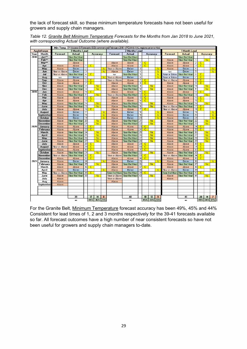
Table 12. Granite Belt Minimum Temperature Forecasts for the Months from Jan 2018 to June 2021, with corresponding Actual Outcome (where available).

For the Granite Belt, Minimum Temperature forecast accuracy has been 49%, 45% and 44% Consistent for lead times of 1, 2 and 3 months respectively for the 39-41 forecasts available so far. All forecast outcomes have a high number of near consistent forecasts so have not been useful for growers and supply chain managers to-date.

30

To obtain the best advantage from a long lead time forecast, the first available forecast needs to be accurate. Tables 13 and 14 list the date and accuracy of the first available Minimum Temperature forecasts to-date.

Table 13. Lockyer Valley Minimum Temperature – First Available Forecast – 3 Month Lead-time.

For the Lockyer Valley Minimum Temperature, a forecast accuracy of 31% Consistent was achieved for the 3 month long lead time forecast based on only the first available monthly forecast for minimum temperatures. The first long lead time forecast has not been useful for

31

growers and supply chain managers in this region, based on the assessment of the 39 forecasts above.

Table 14. Granite Belt Minimum Temperature – First Available Forecast – 3 Month Lead-time.

For the Granite Belt, a forecast accuracy of 38% Consistent was achieved for the 3 month long lead time forecast based on only the first available monthly forecast for minimum temperatures. The number of consistent and near consistent forecasts, highlights the reduced underlying forecast skill. These minimum temperature forecasts have not been

32

useful for growers and supply chain managers, based on assessment of the forecasts issued since January 2018.

Conclusion (Minimum Temperature) For both the Lockyer Valley and Granite Belt, Minimum Temperature forecast accuracy has been made up of a high proportion of Near Consistent forecasts for lead times of 1, 2 and 3 months for the 39-41 forecasts available to-date. These minimum temperature forecasts have not been useful for growers and supply chain managers,based on assessment of the forecasts issued since January 2018.

Both the Lockyer Valley and Granite Belt 3 month long lead time forecasts based on only the first available monthly minimum temperature forecast has been made up of a high proportion of Near Consistent forecasts so have not been useful for growers and supply chain managers,based on assessment of the forecasts issued since January 2018.

Rainfall Forecasts (Tables 15-18) Table 15. Lockyer Valley Rainfall Forecasts for the Months from Jan 2018 to June 2021, with corresponding Actual Outcome (where available).

For the Lockyer Valley, Rainfall forecast accuracy has been 63%, 45% and 54% Consistent for lead times of 1, 2 and 3 months respectively for the 39-41 forecasts available so far, and

33

the number of “Near or Above & Near or Below” forecasts is quite high, decreasing the usefulness of the 2 and 3 month long lead time forecasts for growers and supply chain managers.

The 1 month lead time rainfall forecasts for the Lockyer Valley are more accurate (63% Consistent) and more useful than the 2 & 3 month lead times, based on assessment of the forecasts issued since January 2018.

Table 16. Granite Belt Rainfall Forecasts for the Months from Jan 2018 to June 2021, with corresponding Actual Outcome (where available).

For the Granite Belt, Rainfall forecast accuracy has been 68%, 55% and 49% Consistent for lead times of 1, 2 and 3 months respectively for the 39-41 forecasts available so far, and the number of “Near or Above” and “Near or Below” forecasts is quite high. The 1 month lead time Granite Belt rainfall forecast is showing some skill (68% Consistent) and could be useful while the 2 and 3 month forecasts have not been useful for growers and supply chain managers (based on assessment of the forecasts issued since January 2018.

34

To obtain the best advantage from a long lead time forecast, the first available forecast needs to be accurate. Tables 17 and 18 list the date and forecast accuracy of the first available Rainfall forecasts for the past 41 months.

Table 17. Lockyer Valley Rainfall – First Available Forecast – 3 Month Lead-time.

For the Lockyer Valley, a Rainfall forecast accuracy of 37% Consistent was achieved for the 3 month long lead time forecast based on only the first available monthly forecast for Rainfall. The number of near consistent forecasts in all monthly forecast periods highlights the reduced underlying skill. These 3 month long lead time rainfall forecasts have not been

35

useful for growers and supply chain managers, based on assessment of the forecasts issued since January 2018.

Table 18. Granite Belt Rainfall – First Available Forecast – 3 Month Lead-time.

For the Granite Belt, a Rainfall forecast accuracy of 34% consistent was achieved for the 3 month long lead time forecast based on only the first available monthly forecast Rainfall. The number of near consistent forecasts in all monthly forecast periods highlights the reduced underlying forecast skill. The Granite Belt 3 month long lead time forecast based on

36

the first available forecast of the month is not useful for growers and supply chain managers in this region, based on assessment of all forecasts issued since January 2018.

37

Appendix 2 Significance testing and forecast assessment

Introduction The focus of the project is the assessment of real-time forecasts from ACCESS-S1 via the web site http://poama.bom.gov.au/access-s1/dcap2/1. This provides products tailored to DCAP2#7 researchers in the form of pie charts expressing the probability of forecasts above, below or near the average and daily distributions. Forecasts range from weeks to months to seasons for rainfall, and maximum and minimum temperature. Two forecast regions, Lockyer Valley and Granite Belt, are considered and forecasts for growers are produced every two months for month 1, month 2 and month 3. Interpreting the information available for growers and assessing the truthfulness of the forecast is the key output of the project and must be undertaken consistently. This report discusses the approach that we have developed to address this.

Method

Interpretation of pie charts A typical set of pie charts for maximum temperature in the Lockyer Valley is presented in Figure 1. The pie charts are derived by considering the outcome of the ensemble of 99 runs that are compared to the climatology from 1990 to 2012. Each run represents subtle changes in starting conditions as it is well known that in a chaotic system starting conditions play an important role. In a situation where there is a strong driver acting on the modelled climate, we would hope to see that the outcomes are consistent, i.e., above, below or near the average. It is the magnitude of deviation from a random distribution that we can use to say the odds have shifted in favour of a particular outcome or not. In some of the charts (Figure 1) e.g., Month 1, 2 and 3, it emphatically indicates that there is greater probability of being in the above average tercile and only a small probability that it will be in the below average tercile. However, for Week 2 it suggests that the probability of being in the above average tercile is 19%, with 41% of the forecasts indicating below average. Is this a significant change in the odds of above average temperatures? Consider instead Weeks 2 and 3 where the probability for above average is 36% and below average is 31%. Is this significant? To answer this, we can consider if the forecast probabilities are different from random. If the climate model was acting randomly then there would be an equal likelihood that there would be 33 runs above, 33 runs below and 33 runs near the average. A Chi2 test (χ2) can be used to test if the outcome is significantly different from random.

1 This site is password protected

38

Figure 11. Maximum temperature pie charts for a forecast made on 8 June 2019.

Statistical analyses of individual pie charts shown in Figure 1. The pie charts are expressed as percent, i.e., out of 100, but in order to calculate our Observed number of ensembles we must multiply the percentage by 99/100. This makes a small difference to our values in this case, but in situations where we are assessing the hindcast series that comprise 11-run ensembles this is an important step and necessary as we do not have direct access to the datasets. The process is laid out below:

𝜒𝜒2 = �(𝑂𝑂 − 𝐸𝐸)2

𝐸𝐸

where O is observed, E is expected. Week 2

Tercile Percentage from pie chart

Observed number of runs3

Expected number of runs1

Chi2 values

Near Average 39 (40)2 39.6 33 1.3200 Above Average

19 18.10 33 6.1017

Below Average

41 40.59 33 1.7457

Total 100 99 99 9.1674

39

1. The expected number of runs in each of three categories for a 99-run ensemble is

33. 2. Percentages shown on the pie chart do not show decimal places, so there is a

rounding error. 3. Given note 2, this is now a derived number of observations, aka a workaround.

In this example the χ2 value is 9.17 and this compared to χ2 distribution with 2 degrees of freedom. Since the calculated value, 9.17, is greater than the tabulated value, 5.99, we conclude that the distribution of percentages is unlikely to have arrived by randomness. In fact, the p-value is 0.01 and the likelihood of above average temperatures during week 2 is significant.

Undertaking the same calculations for Weeks 2 and 3 shows that the calculated χ2 value is 0.38 and the p value is 0.8. The distribution of the outcomes from the ensembles is equal across the terciles. In this case the odds in favour of any tercile are not changed. This does not imply that we would expect average conditions, but rather below, above and near average outcomes are equally likely. Remember that here we are looking at 99 possible outcomes, but there will only be one point of truth. An Excel spreadsheet function was developed to undertake these calculations.

Interpretation of daily distributions The other set of information that we have to work with is the daily distribution of values from the forecast for a given period and duration. The relevant distributions for Week 2 and Week 3 are shown Figure 2.

Figure 12. Daily distribution of forecasted values and climatology for Week 2 (left) and Weeks 2 and 3 (right).

Interpretation of these distributions can be done visually by comparing the forecasted values (mustard colour) with the climatology (grey). For Week 2 there is an increase in the number of days in the 16°C to 18°C range and fewer in the 22°C to 24°C range. This is consistent with the information shown in the pie chart for that period. Similarly, for Weeks 2 and 3, the

40

distribution is consistent with the pie chart that did not favour one tercile over the other. While this might seem to be the opposite to the discussion above and that the forecast is for climatology, in fact, these distributions show an average for the 99 runs. In that respect the message from the forecast is the same – we have no indication that there will be increase or decrease in the likelihood of one tercile over another and management decisions should be based on climatology. When we have a significant result from the pie chart, we can explore the magnitude of that shift using the tercile boundaries from climatology. These have been calculated for each region using the AWAP2 data provided by the BoM. If the mean value is less than the lower tercile than we have a significant decrease and an increase if the mean is greater than the upper tercile. Otherwise the forecast is in the near average region. Consider the forecast for March 2019 issued on 8 February 2019, Figure 3.

Figure 13. Pie chart and daily distribution forecast of maximum temperature for Lockyer Valley for March 2019 issued on 8 February 2019.

The pie chart in Figure 3 shows an emphatic forecast for maximum temperatures in the above average tercile and the distribution shows a marked shift to the right (hotter temperatures). The forecast mean is 30.4°C and the tercile range calculated for March for the Lockyer Valley, is 28.5°C to 29.8°C, Table 1. The forecast mean is greater than the upper tercile and we conclude that there is a significant shift in the mean.

2 AGCD – The Australian Gridded Climate Data. Also known as AWAP as it was initiated under the Australian

Water Availability Project.

41

Combining the two pieces of information, the pie chart and the distribution, provides as thorough an assessment that can be made using the outputs provided. Table 1. Mean maximum temperature and lower and upper tercile boundaries for the Lockyer Valley region.

Month Mean Lower Upper January 31.3 31.1 31.9 February 30.4 29.8 30.9 March 29.2 28.5 29.8 April 26.9 26.6 27.5 May 23.7 23.3 24.0 June 21.1 20.6 21.5 July 20.8 20.4 21.0 August 22.6 22.3 22.9 September 25.8 25.0 26.1 October 27.9 27.5 28.2 November 29.7 29.3 30.5 December 30.9 30.4 31.6

Discussion The original intention within the project was to provide clients with access to the web page so that they can interpret the forecasts themselves. It quickly became apparent that using the website in its current format was not a good use of their time, due to the complexity of interpretation. The use of the Chi2 test provided a simple statistic to judge the forecast to avoid call the result for a particular category when in fact there was no difference between them.

42

Appendix 3

Verification of gridded data sets using field measurements

Introduction

The focus of the project is the assessment of real-time forecasts from ACCESS-S1 via the web site http://poama.bom.gov.au/access-s1/dcap2/3. This provides products tailored to DCAP2#7 researchers in the form of pie charts expressing the probability of forecasts above, below or near the average and daily distributions. Forecasts range from weeks to months to seasons for rainfall, and maximum and minimum temperature. Two forecast regions, Lockyer Valley and Granite Belt, are considered and forecasts for growers are produced every two months for month 1, month 2 and month 3. Interpreting the information available for growers and assessing the truthfulness of the forecast is the key output of the project and must be undertaken consistently. The ACCESS-S1 operates at a scale of 60 km over land, however, these are then downscaled to a 5 km grid using the Bureau of Meteorology’s AGCD (Australian Gridded Climate Data) from the Australian Water Availability Project (AWAP). In keeping with convention, the report will refer to these as the AWAP grids. These gridded data sets have an impact on the derivation the forecast outputs and there was an opportunity to examine how closely the gridded data agreed with on-farm measurements. This was undertaken for maximum and minimum daily temperature and monthly rainfall.

Method

Daily Gridded Data from AWAP This analysis was undertaken using the AWAP data for each day, accessed using the Maps – recent conditions section of the BoM website (http://www.bom.gov.au/climate/maps/, Figure 1). This is the 5km grid used to downscale outputs from ACCESS-S1. The option Grid can be used to download a data set for each day, and these were obtained for October 2020 to June 2021 for maximum and minimum temperatures and rainfall. The AWAP grids use the ESRI grid data format and was read using the R package raster, version 3.4-13 (https://rspatial.org/). All subsequent analysis was undertaken in R.

3 This site is password protected. Some of the products that were available will become part of the operational

data service provided by BoM.

43

Figure 14. Partial screen shot of the daily maximum temperature for 4 July 2021.

The data for the Granite Belt and Lockyer Valley was extracted and compared to field measurements from our weather stations and the BoM AWS station (Figure 2). Three weather stations (BHSystems, Brisbane, Queensland) were established within the Granite Belt (Figure 2, labelled M1 – M3) and one in the Lockyer Valley, near Lowood. Data from these stations and the Applethorpe and University of Queensland, Gatton AWS provided six “points of truth” to compare to AWAP grid. Two measures were used to assess the agreement between grid cell data and weather station. The correlation coefficient (R) measures the amount agreement between the two data sets where values of 0 represent no agreement and 1 perfect agreement. The RMSE (root mean square error) measures the error across all data points. Here a lower value is better, and the units are °C.

44

Figure 15. Maximum Temperature for Granite Belt Region for 4 July 2021. Grid shows the region used for Granite Belt forecasts from ACCESS-S1

Results

The analysis was undertaken for daily minimum and maximum temperature, daily and monthly rainfall. In each case the value recorded at the weather station was compared with the value from the cell.

Maximum Temperature

Maximum temperatures recorded from the grid cells were in close agreement with those recorded at the weather station in the Granite Belt and Lockyer Valley. The site at Amiens recorded the highest error at 1.32°C, Figure 3. For the two stations in the Lockyer Valley, the RMSE were less than 1°C Figure 4.

45

Figure 16. Correlation between maximum temperature recorded at the weather station and the corresponding AWAP grid cell for the Granite Belt.

Figure 17 Correlation between maximum temperature recorded at the weather station and the corresponding AWAP grid cell for the Lockyer Valley.

Minimum Temperature

The relationship between weather station and grid cells was not as close as for maximum temperatures. Except for the Applethorpe AWS the RMSE was greater than 1°C. Minimum temperatures are more affected by local conditions at scale less than can be incorporated within a 5 km grid. This perhaps explains some of the lower skill seen in the forecasts, Figure 5 and Figure 6.

46

Figure 18 Correlation between minimum temperature recorded at the weather station and the corresponding AWAP grid cell for the Granite Belt

Figure 19 Correlation between minimum temperature recorded at the weather station and the corresponding AWAP grid cell for the Lockyer Valley

Rainfall

While the rainfall forecasts at the regional scale showed some skill, the correlation between daily rainfall amounts recorded at the station and the grid cell. The correlation at sites within the Granite Belt ranged from to 0.53 and 0.66, although the Applethorpe AWS was 0.84, in the Lockyer Valley they were 0.59 and 0.44. Monthly totals were examined and as can be seen from there was more variability between stations and generally the grid data

47

overestimated the rainfall.

Figure 20. Monthly rainfall totals for Granite Belt weather stations

Figure 21 Monthly rainfall totals for Granite Belt for corresponding grid cells

Discussion

The analysis showed that there was a high correlation between the weather station maximum temperature recording and the value that came from the AWAP grid. The relationship was weaker for minimum temperature and not reliable for rainfall. There was a good relationship for monthly totals for rainfall.