Using Blind Search and Formal Conceptsfor Binary Factor Analysis

Ales Keprt

Dept. of Computer Science, FEI, VSB Technical University Ostrava, Czech Republicales.keprt@vsb.cz

Abstract. Binary Factor Analysis (BFA, also known as Boolean FactorAnalysis) may help with understanding collections of binary data. Sincewe can take collections of text documents as binary data too, the BFAcan be used to analyse such collections. Unfortunately, exact solving ofBFA is not easy. This article shows two BFA methods based on exactcomputing, boolean algebra and the theory of formal concepts.

Keywords: Binary factor analysis, boolean algebra, formal concepts

1 Binary factor analysis

1.1 Problem definition

To describe the problem of Binary Factor Analysis (BFA) we can paraphraseBMDP’s documentation (Bio-Medical Data Processing, see [1]).

BFA is a factor analysis of dichotomous (binary) data. This kind of analysisdiffers from the classical factor analysis (see [16]) of binary valued data, eventhough the goal and the model are symbolically similar. In other words, bothclassical and binary analysis use symbolically the same notation, but their sensesare different.

The goal of BFA is to express p variables X = (x1, x2, . . . , xp) by m factors(F = f1, f2, . . . , fm), where m � p (m is considerably smaller than p). Themodel can be written as

X = F �A

where � is matrix multiplication. For n cases, data matrix X, factor scores F ,and factor loadings A can be written asx1,1 . . .x1,p

.... . .

...xn,1. . .xn,p

=

f1,1 . . .f1,m

.... . .

...fn,1. . .fn,m

�a1,1 . . . a1,p

.... . .

...am,1. . .am,p

where elements of all matrices are valued 0 or 1 (i.e. binary).

c© V. Snasel, J. Pokorny, K. Richta (Eds.): Dateso 2004, pp. 128–140, ISBN 80-248-0457-3.VSB – Technical University of Ostrava, Dept. of Computer Science, 2004.

Using Blind Search and Formal Concepts for Binary Factor Analysis 129

1.2 Difference to classical factor analysis

Binary factor analysis uses boolean algebra, so matrices of factor scores andloadings are both binary. See the following example: The result is 2 in classicalalgebra

[1 1 0 1] ·

1100

= 1 · 1 + 1 · 1 + 0 · 0 + 1 · 0 = 2

but it’s 1 when using boolean algebra.

[1 1 0 1] ·

1100

= 1 · 1⊕ 1 · 1⊕ 0 · 0⊕ 1 · 0 = 1

Sign ⊕ marks disjunction (logical sum), and sign · mars conjunction (logicalconjunction). Note that since we focus to binary values, the logical conjunctionis actually identical to the classic product.

In classical factor analysis, the score for each case, for a particular factor, is alinear combination of all variables: variables with large loadings all contribute tothe score. In boolean factor analysis, a case has a score of one if it has a positiveresponse for any of the variables dominant in the factor (i.e. those not havingzero loadings) and zero otherwise.

1.3 Success and discrepancy

It is obvious, that not every X can be expressed as F �A. The success of BFA ismeasured by comparing the observed binary responses (X) with those estimatedby multiplying the loadings and the scores (X = F �A). We count both positiveand negative discrepancies. Positive discrepancy is when the observed value (inX) is one and the analysis (in X) estimates it to be zero, and reversely negativediscrepancy is when the observed value is zero and the analysis estimates it tobe one. Total count of discrepancies d is a suitable measure of difference betweenobserved values xi,j and calculated values xi,j .

d =n∑

i=1

p∑j=1

|xi,j − xi,j |

1.4 Terminology notes

Let’s summarize the terminology we use. Data to be analyzed are in matrix X.Its columns xj represent variables, whereas its rows xi represent cases. The

130 Ales Keprt

factor analysis comes out from the generic thesis saying that variables, we canobserve, are just the effect of the factors, which are the real origin. (You canfind more details in [16].) So we focus on factors. We also try to keep number offactors as low as possible, so we can say ”reducing variables to factors”.

The result is the pair of matrices. Matrix of factor scores F expresses theinput data by factors instead of variables. Matrix of factor loadings A definesthe relation between variables and factors, i.e. each row ai defines one particularfactor.

1.5 An example

As a basic example (see [1]) we consider a serological problem1, where p tests areperformed on the blood of each of n subjects (by adding p reagents). The outcomeis described as positive (a value of one is assigned for the test in data matrix),or negative (zero is assigned). In medical terms, the scores can be interpreted asantigens (for each subject), and the loading as antibodies (for each test reagent).See [14] for more on these terms.

1.6 Application to text documents

BFA can be also used to analyse a collection of text documents. In that case thedata matrix X is built up of a collection of text documents D represented as p-dimensional binary vectors di, i ∈ 1, 2, . . . , n. Columns of X represent particularwords. Particular cell xi,j equals to one when document i contains word j, andzero otherwise. In other words, data matrix X is built in a very intuitive way.

It should be noted that some kind of smart (i.e. semantic) preprocessingcould be made in order to let the analysis make more sense. For example weusually want to take world and worlds as the same word. Although the binaryfactor analysis has no problems with finding this kind similarities itself, it iscomputationally very expensive, so any kind of preprocessing which can decreasethe size of input data matrix X is very useful. We can also use WordNet, orthesaurus to combine synonyms. For additional details see [5].

2 The goal of exact binary factor analysis

In classic factor analysis, we don’t even try to find 100% perfect solution, be-cause it’s simply impossible. Fortunately, there are many techniques that give agood suboptimal solution (see [16]). Unfortunately, these classic factor analysistechniques are not directly applicable to our special binary conditions. Whileclassic techniques are based on the system of correlations and approximations,

1 Serologic test is a blood test to detect the presence of antibodies against microor-ganism. See serology entry in [14].

Using Blind Search and Formal Concepts for Binary Factor Analysis 131

these terms can be hardly used in binary world. Although it is possible to applyclassic (i.e. non-boolean non-binary) factor analysis to binary data, if we reallyfocus to BFA with restriction to boolean arithmetic, we must advance anotherway.

You can find the basic BFA solver in BMDP – Bio-Medical Data Processingsoftware package (see [1]). Unfortunately, BMDP became a commercial product,so the source code of this software package isn’t available to the public, and eventhe BFA solver itself isn’t available anymore. Yet worse, there are suspicionssaying that BMDP’s utility is useless, as it actually just guesses the F andA matrices, and then only explores the similar matrices, so it only finds localminimum of the vector error function.

One interesting suboptimal BFA method comes from Husek, Frolov et al.(see [15], [7], [6], [2], [8]). It is based on a Hopfield-like neural network, so it findsa suboptimal solution. The main advantage of this method is that it can analysevery large data sets, which can’t be simply processed by exact BFA methods.

Although the mentioned neural network based solver is promising, we actu-ally didn’t have any one really exact method, which could be used to proof theother (suboptimal) BFA solvers. So we started to work on it.

3 Blind search based solver

The very basic algorithm blindly searches among all possible combinations of Fand A. This is obviously 100% exact, but also extremely computational expen-sive, which makes this kind of solver in its basic implementation simply unusable.

To be more exact, we can express the limits of blind search solver in unitsof n, p and m. Since we need to express matrix X as the product of matricesF � A, which are n ×m and m × p in size, we need to try on all combinationsof m · (n + p) bits. And this is very limiting, even when trying to find only3 factors from 10 × 10 data set (m = 3, n = 10, p = 10), we end up withcomputational complexity of 2m·(n+p) = 260, which is quite behind the scope ofcurrent computers.

4 Revised blind search based solver

In order to make the blind search based solver more usable, we did severalchanges to it.

4.1 Preprocessing

We must start with optimizing data matrix. The optimization consist of thesesteps:

132 Ales Keprt

Empty rows or columns All empty rows and empty columns are removed,because they has no effect on the analysis. Similarly, the rows and columns full ofone’s can be removed too. Although removing rows and columns full of one’s canlead to higher discrepancy (see sec. 1.3), it doesn’t actually have any negativeimpact on the analysis.

Moreover, we can ignore both cases (rows) and variables (columns) with toolow or too high number of one’s, because they are usually not very importantfor BFA. Doing this kind of optimization can significantly reduce the size ofdata matrix (directly or indirectly, see below), but we must be very careful,because it can lead to wrong results. Removing too many rows and/or columnsmay completely degrade the benefit of exact BFA, because it leads to exactcomputing with inexact data. In regard to this danger, we actually implementedonly support for removing columns with too low number of one’s.

Duplicate rows and columns With duplicate rows (and columns resp.) arethe ones which are the same to each other. Although this situation can hardlyappear in classic factor analysis (meaning that two measured cases are 100%identical), it can happen in binary world much easier, and it really does. As forduplicate rows, the main reason of their existence is usually in the preprocessing.If we do some kind of semantic preprocessing, or even forcibly remove somecolumns with low number of one’s, the same (i.e. duplicate) rows occur. Wecan remove them without negative impact to the analysis, if we remember therepeat-count of each row. We call it multiplicity.

Then we can update the discrepancy formulae (see sec. 1.3) to this form:

d =n∑

i=1

p∑j=1

(mRi ·mC

j |xi,j − xi,j |)

where mRi and mC

j are multiplicity values for row i and column j respectively.We can also compute the multiplicity matrix M :

M =

m1,1 . . .m1,p

.... . .

...mn,1. . .mn,p

where mi,j = mR

i · mCj . Although this leads to simpler and better readable

formulae

d =n∑

i=1

p∑j=1

(mi,j |xi,j − xi,j |)

it isn’t a good idea, since the implementation is actually inefficient, since it needsa lot of additional memory (n · p numbers compared to n + p ones).

The most important note is, that the merging of duplicate rows and columnslead to a significant reduction in computation time, and still doesn’t bring anyerrors to the computation.

Using Blind Search and Formal Concepts for Binary Factor Analysis 133

4.2 Bit-coded matrices

Using standard matrices is simple, because it is based on classic two-dimensionalarrays and makes the source code well readable. In contrast, we also implementedthe whole algorithm using bit-coded matrices and bitwise (truly boolean) oper-ations (like and, or, xor). That resulted in not so nice source code, and alsorequired some tricks, but also saved a lot of computation speed. We actuallysped up the code by 20% by using bit-coded matrices and bitwise (boolean)operations.

4.3 The strategy

Although all the optimizations presented above lead to lower computation time,it is still not enough. To save yet more computation time, we need a goodstrategy.

The main problem is that we need to try too many bits in matrices F andA. Fortunately there exist a way of computing one of these matrices from theother one, thanks to knowing X. Since we are more concerned in A, we checkout all bits in that one, and then find the right F . In summary:

1. Build up one particular candidate for matrix A.2. Find the best F for this particular A.3. Multiply these matrices and compare the result with X. If the discrepancy

is smaller to the so far best one, remember this F,A pair.4. Back to step 1.

After we go through all possible candidates for A, we’re done.

4.4 Computing F from A and X

Symbolically, we can express this problem as follows. We are trying to find Fand A, so X = F � A. Let we know X and A, so we only need to computeF . If we take a parallel from numbers, we can write something like F = X/A.Unfortunately, this operation isn’t possible with common binary matrices.

If we bit-code matrices X and A on row-by-row basis, so X = [x1, . . . , xn]T

and A = [a1, . . . ap]T , then

xi =m∑

k=1

fi,k · aj

From this formulae we can compute F on row-by-row basis, which signif-icantly speeds up whole algorithm. The basic idea still relies on checking outall bit combinations for each row of F , which is 2m · m in total, but we canpossibly find a better algorithms in future. In our implementation we computediscrepancy together with finding F , so we can abort the search whenever the

134 Ales Keprt

partial discrepancy is higher than the so far best solution. This way we get somespeedup which could be made yet higher by pre-sorting rows of A by the dis-crepancies caused by particular rows, etc. Exploration of these areas isn’t veryimportant, because the possible speedup is quite scanty.

Note that in this place we can also focus to positive or negative discrepancyexclusively. It can be done using boolean algebra without any significant speedpenalties.

5 Parallel implementation

The bind-search algorithm (including the optimized version presented above)can exploit the power of parallel computers (see [9]). We used PVM interface(Parallel Virtual Machine, see [4]) which is based on sending messages. The BFAblind search algorithm is very suitable for this kind of parallelism, because wejust need to find a smart way of splitting the space of possible solutions to bechecked out to a set of sub-spaces, and distribute them among available processorin our parallel virtual machine.

We tested this method using 2 to 11 PC desktop computers on a LAN (localarea network). We managed to gain the absolute efficiency around 92%2, whichis very high compared to usual parallel programs. (The number 92% says thatit takes 92% of time to run 11 consecutive runs on the same data, compared toa single run of the parallel version on the network of 11 computers).

6 Concept lattices

Another method of solving BFA problem is based on concept lattices. This sec-tion gives minimum necessary introduction to concept lattices, and especiallyconcepts, which are the key part of the algorithm.

Definition 1 (Formal context, objects, attributes).Triple (X, Y,R), where X and Y are sets, and R is a binary relation R ⊆ X×Y ,is called formal context. Elements of X are called objects, and elements ofY are called attributes. We say ”object A has attribute B”, just when A ⊆ X,B ⊆ Y and (A,B) ∈ R. ut

Definition 2 (Derivation operators).For subsets A ⊆ X and B ⊆ Y , we define

A↑ = {b ∈ B | ∀a ∈ A : (a, b) ∈ R}B↓ = {a ∈ A | ∀b ∈ B : (a, b) ∈ R}

ut2 It was measured in Linux, while Windows 2000 performed a bit worse and its per-

formance surprisingly fluctuated.

Using Blind Search and Formal Concepts for Binary Factor Analysis 135

In other words, A↑ is the set of attributes common to all objects of A, andsimilarly B↓ is the set of all objects, which have all attributes of B.

Note: We just defined two operators ↑ and ↓:

↑ : P (X) → P (Y )↓ : P (Y ) → P (X)

where P (X) and P (Y ) are sets of all subsets of X and Y respectively.

Definition 3 (Formal concept).Let (X, Y,R) be a formal context. Then pair (A,B), where A ⊆ X, B ⊆ Y ,A↑ = B and B↓ = A, is called formal concept of (X, Y,R).

Set A is called extent of (A,B), and set B is called intent of (A,B). ut

Definition 4 (Concept ordering).Let (A1, B1) and (A2, B2) be formal concepts. Then (A1, B1) is called subconceptof (A2, B2), just when A1 ⊆ A2 (which is equivalent to B1 ⊇ B1). We write(A1, B1) ≤ (A2, B2). Reversely we say, that (A2, B2) is superconcept of (A1, B1).

ut

In this article we just need to know the basics of concepts and their meaning.For more detailed, descriptive, and well understandable introduction to FormalConcept Analysis and Concept Lattices, see [3], [11] or [13].

7 BFA using formal concepts

If we want to speed up the simple blind-search algorithm, we can try to findsome factor candidates, instead of checking out all possible bit-combinations.The technique which can help us significantly is Formal Concept Analysis (FCA,see [11]). FCA is based on concept lattices, but we actually work with formalconcepts only, so the theory we need is quite simple.

7.1 The strategy

We can still use some good parts of the blind-search program (matrix optimiza-tions, optimized bitwise operations using boolean algebra, etc.), but instead ofchecking out all possible bit combinations, we work with concepts as the factorcandidates. In addition, we can adopt some strategy optimizations (as discussedabove) to concepts, so the final algorithm is quite fast; its strength actually relieson the concept-building algorithm we use.

136 Ales Keprt

So the BFA algorithm is then as follows:

1. Compute all concepts of X. (We use a standalone program to do this.)2. Import the list of concepts, and optimize it, so it correspond to our optimized

data matrix X. (This is simple. We just merge objects and attributes thesame way, as we merged duplicate rows and columns of X respectively.)

3. Remove all concepts with too many one’s. (The number of one’s per factoris one of our starting constraints.)

4. Use the remaining concepts as the factor candidates, and find the best m-element subset (according to discrepancy formulae).

This way we can find the BFA solution quite fast, compared to the blindsearch algorithm. Although the algorithm described here looks quite simple3,there is a couple of things, we must be aware of.

7.2 More details

The most important FCA consequence is that 100% correct BFA solution canalways be found among all subsets of concepts. This is very important, becauseit is the main guarantee of the correctness of the concept based BFA solver.

Other important feature of FCA based concepts is that they never directlygenerate any negative discrepancy. It is a direct consequence of FCA qualities,and affects the semantic sense of the result. As we discussed above (and see also[1]), negative discrepancy is a case when F �A gives 1 when it should be 0. Fromsemantic point of view, this (the negative discrepancy) is commonly unwantedphenomenon. In consequence, the fact that there’s no negative discrepancy inthe concepts, may have negative impact on the result, but the reality is usuallyright opposite. (Compare this to the quick sort phenomenon.)

The absence of negative discrepancies coming from concepts applies to Amatrix only. It doesn’t apply to F matrix, we still can use any suitable valuesfor it. In consequence, we always start with concepts not generating negativediscrepancy, which are semantically better, and end up with best suitable factorscores F , which give the lowest discrepancy. So it seems to be quite good feature.

7.3 Implementation issues

It’s clear that the data matrix X is usually quite large, and makes the findingof the formal concepts the main issue. Currently we use the standalone CL(concept lattice) builder. It is optimized for finding concept lattices, but that’snot right what we need. In the future, we should consider adopting some kindof CL building algorithm directly into BFA solver. This will save a lot of time

3 Everything’s simple, when you know it.

Using Blind Search and Formal Concepts for Binary Factor Analysis 137

when working with large data sets, because we don’t need to know the concepthierarchy.

We don’t even need to know all the formal concepts, because the startingconstraints limit the maximum number of one’s in a factor, which is directlyapplicable to CL building.

8 Comparing the results and the computation times

The two algorithms presented in this article were tested on the test data suitetaken from the neural algorithm mentioned above (see [15], [7], [6], [2], [8]). Wefocused to test data sets p2 and p3, which are both 100× 100 values in size, anddiffers in the ones’ density. All three algorithms gave the same results, so theyall appear to be correct (from this point of view).

Table 1. Computation times

data set factors one’s time (m:s) discrepancy notes

p3.txt 5 2–4 61:36 0 375 combinationsp3.txt 5 3 0:12 0 120 combinationsp3.txt 5 1–10 0:00 0 8/10 concepts

p2.txt 2 6 11:44 743 54264 combinationsp2.txt 5 1–10 0:07 0 80/111 conceptsp2.txt 5 6–8 0:00 0 30/111 concepts

The results are shown in table 8. Data set p3 is rather simple, its factor load-ings (particular rows of A) all have 3 one’s. The first row in the table shows thatit takes over 61 minutes to find these factors, when we search all combinationswith 2, 3 or 4 one’s per factor. If we knew that there are just 3 one’s per factor,we can specify it as a constraint, and we get the result in just 12 seconds (seetable 1, row 2). Indeed we usually don’t know it in real situations.

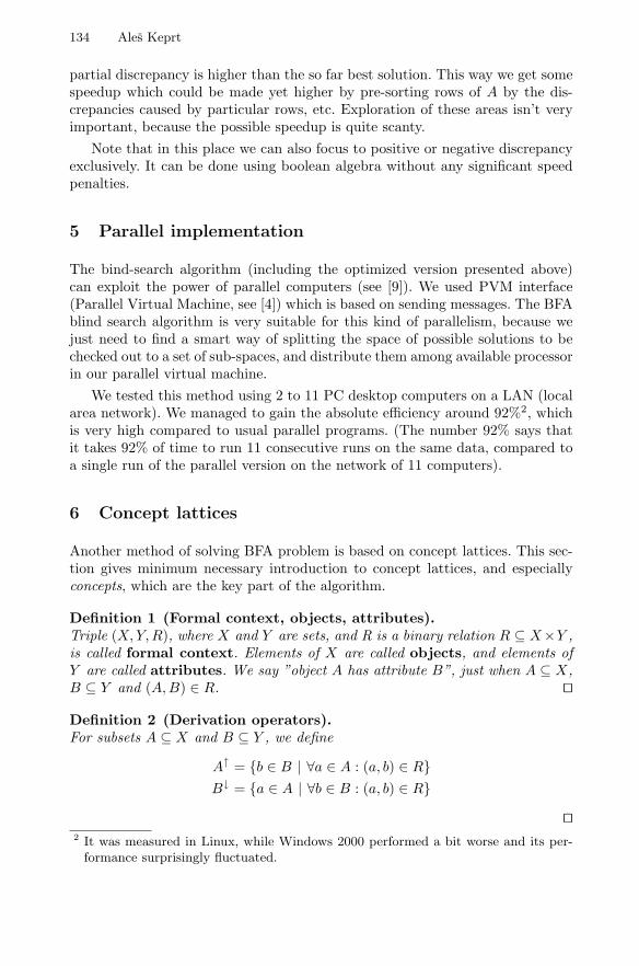
Third row shows that when using formal concepts, we can find all factors injust 0 seconds, even when we search all possible combinations with 1 to 10 one’sper factor. You can see the concept lattice in picture 1, with factors expressivelycircled.

Data set p2 is much more complex, because it is created from factors con-taining 6 one’s each. In this case the blind-search algorithm was able to find just2 factors. It took almost 12 minutes, and discrepancy was 743. In addition, thetwo found factors are wrong, which is not a surprise according to the fact thatthere are actually 5 factors, and they can’t be searched individually. It was notpossible to find more factors using blind-search algorithm. Estimated times forcomputing 3 to 5 factors with the same constraints (limiting number of one’sper factor to 6) are shown in table 8. It shows that it would take up to 3.5×109

years to find all factors. Unfortunately, we can’t afford to wait so long. . .

138 Ales Keprt

0a

0

100o

1a

77

77o

2a

84

42o

1a

36

36o

3a

69

23o

3a

69

23o

3a

66

22o

3a

57

19o

3a

39

13o

30a

0

0o

Fig. 1. Concept lattice of p3 data set.

Table 2. Estimated computation times

data set factors one’s estimated time

p2.txt 3 6 440 daysp2.txt 4 6 65700 yearsp2.txt 5 6 3.5×109 years

As you can see at the bottom of table 1, we can find all 5 factors of p2 easilyin just 7 seconds, searching among candidates containing 1 to 10 one’s. The timecan be reduced to 0 seconds once again, if we reduce searching to the range of 6to 8 one’s per factor. You can see the concept lattice in picture 1, with factorsmarked as well. As you can see, the factors are non-overlapping, i.e. they arenot connected to each other. Note that this is not a generic nature. Generally,factors can arbitrarily overlap.

9 Conclusion

This article presented two possible algorithms for exact solving of Binary FactorAnalysis. The work on them originally started as a simple blind search algorithmin order to check out the results of P8M of BMDP (see [1]), and the promisingneural network solver (see [15], [7], [6], [2], [8]). As the work progressed, thetheory of Concept Lattices and Concept Analysis was partially adopted into it,and it was with an inexpectably good results. For sure, the future work will more

Using Blind Search and Formal Concepts for Binary Factor Analysis 139

2a200

100o3a

282

94o

3a

279

93o

3a

264

88o4a348

87o

3a

258

86o

3a

258

86o4a328

82o

4a324

81o

4a320

80o

4a320

80o

4a316

79o

4a316

79o5a

375

75o

4a296

74o

4a296

74o5a

365

73o

5a

365

73o

4a288

72o5a

340

68o

5a

340

68o

7a

469

67o

5a

335

67o

5a

335

67o

5a

330

66o

5a

325

65o

6a372

62o8a

496

62o

6a

366

61o

6a

366

61o

5a

300

60o6a

354

59o

7a

392

56o

8a

44055o

6a

33055o

9a

495

55o

7a

38555o

7a

378

54o6a

324

54o

8a

42453o

6a

318

53o

8a

42453o

7a

350

50o7a

343

49o

8a

392

49o

9a

432

48o

8a

384

48o9a

432

48o

7a

336

48o7a

329

47o

8a

376

47o8a

352

44o

7a

301

43o

8a

344

43o

8a

336

42o10a410

41o

9a

369

41o

9a

369

41o

8a

328

41o

9a

369

41o10a410

41o

8a

320

40o9a

351

39o9a333

37o

8a296

37o

11a396

36o

8a

288

36o9a315

35o

12a420

35o

12a408

34o

9a

306

34o12a408

34o

10a340

34o

9a

297

33o9a279

31o

9a270

30o

10a290

29o

9a261

29o

12a336

28o

10a270

27o12a

324

27o

13a

351

27o

10a270

27o10a

25025o

12a

288

24o

10a

23023o

11a253

23o

10a230

23o12a

264

22o

13a

273

21o

13a

273

21o

13a

273

21o

13a

26020o

13a

26020o

10a

19019o

11a

187

17o

11a

187

17o

12a

204

17o

12a

19216o

16a

22414o

13a

182

14o16a

22414o

15a195

13o

13a156

12o

16a160

10o

14a140

10o

15a105

7o

15a105

7o

16a

1127o

13a78

6o30a

00o

Fig. 2. Concept lattice of p2 data set.

focus on the possibilities of exploiting formal concepts and concept lattices forBFA.

References

1. BMDP (Bio-Medical Data Processing). A statistical software package. SPSS.http://www.spss.com/

2. A.A.Frolov, A.M.Sirota, D.Husek, I.P.Muraviev, P.A.Polyakov: Binary factoriza-tion in Hopfield-like neural networks: Single-step approximation and computer sim-ulations. 2003.

3. Bernhard Ganter, Rudolf Wille: Formal Concept Analysis: Mathematical Founda-tions. Springer–Verlag, Berlin–Heidelberg–New York, 1999.

4. Al Geist et al.: PVM: Parallel Virtual Machine, A User’s Guide and Tutorial forNetworked Parallel Computing. MIT Press, Cambridge, Massachusetts, USA, 1994.

5. Andreas Hotho, Gerd Stumme: Conceptual Clustering of Text Clusters. In Proceed-ings of FGML Workshop, pp. 37–45. Special Interest Group of German InformaticsSociety, 2002.

6. D.Husek, A.A.Frolov, I.Muraviev, H.Rezankova, V.Snasel, P.Polyakov: Binary Fac-torization by Neural Autoassociator. AIA Artifical Intelligence and Applications -IASTED International Conference, Benalmadena, Malaga, Spain, 2003.

7. D.Husek, A.A.Frolov, H.Rezankova, V.Snasel: Application of Hopfield-like Neu-ral Networks to Nonlinear Factorization. Proceedings in Computational StatisticsCompstat 2002, Humboldt-Universitt, Berlin, Germany, 2002.

140 Ales Keprt

8. D.Husek, A.A.Frolov, H.Rezankova, V.Snasel, A.Keprt: O jednom neuronovemprıstupu k redukci dimenze. In proceedings of Znalosti 2004, Brno, CZ, 2004. ISBN80-248-0456-5.

9. Ales Keprt: Paralelnı resenı nelinearnı booleovske faktorizace. VSB Technical Uni-versity, Ostrava (unpublished paper), 2003.

10. Ales Keprt: Binary Factor Analysis and Image Compression Using Neural Net-works. In proceedings of WOFEX 2003, Ostrava, 2003. ISBN 80-248-0106-X.

11. Christian Lindig: Introduction to Concept Analysis. Hardvard University, Cam-bridge, Massachusetts, USA.

12. Christian Lindig: Fast Concept Analysis. Harvard University, Cambridge, Mas-sachusetts, USA.http://www.st.cs.uni-sb.de/~lindig/papers/fast-ca/iccs-lindig.pdf

13. Christoph Schwarzweller: Introduction to Concept Lattices. Journal Of FormalizedMathematics, volume 10, 1998. Inst. of Computer Science, University of Bialystok.

14. Medical encyclopedia Medline Plus. A service of the U.S. National Library ofMedicine and the National Institutes of Health.http://www.nlm.nih.gov/medlineplus/

15. A.M.Sirota, A.A.Frolov, D.Husek: Nonlinear Factorization in Sparsely EncodedHopfield-like Neural Networks. ESANN European Symposium on Artifical NeuralNetworks, Bruges, Belgium, 1999.

16. Karl Ueberla: Faktorenanalyse (2nd edition). Springer–Verlag, Berlin–Heidelberg–New York, 1971. ISBN 3-540-04368-3, 0-387-04368-3.(slovensky preklad: Alfa, Bratislava, 1974)