USING BAYESIAN NETWORK TO DEVELOP DRILLING EXPERT SYSTEMS

A Dissertation

By

ABDULLAH SALEH H. ALYAMI

Submitted to the Office of Graduate Studies of Texas A&M University

in partial fulfillment of the requirements for the degree of

DOCTOR OF PHILOSOPHY

August 2012

Major Subject: Petroleum Engineering

USING BAYESIAN NETWORK TO DEVELOP DRILLING EXPERT SYSTEMS

Copyright 2012 Abdullah Saleh H. Alyami

USING BAYESIAN NETWORK TO DEVELOP DRILLING EXPERT SYSTEMS

A Dissertation

by

ABDULLAH SALEH H. ALYAMI

Submitted to the Office of Graduate Studies of Texas A&M University

in partial fulfillment of the requirements for the degree of

DOCTOR OF PHILOSOPHY

Approved by:

Chair of Committee, Jerome J. Schubert Committee Members, Hans C. Juvkam-Wold Gene Beck Yuefeng Sun Head of Department, A. Daniel Hill

August 2012

Major Subject: Petroleum Engineering

iii

ABSTRACT

Using Bayesian Network to Develop Drilling Expert Systems.

(August 2012)

Abdullah Saleh H. Alyami, B.S., Florida Institute of Technology; M.S., King Fahd

University of Petroleum and Minerals

Chair of Advisory Committee: Dr. Jerome J. Schubert

Long years of experience in the field and sometimes in the lab are required to

develop consultants. Texas A&M University recently has established a new method to

develop a drilling expert system that can be used as a training tool for young engineers

or as a consultation system in various drilling engineering concepts such as drilling

fluids, cementing, completion, well control, and underbalanced drilling practices.

This method is done by proposing a set of guidelines for the optimal drilling

operations in different focus areas, by integrating current best practices through a

decision-making system based on Artificial Bayesian Intelligence. Optimum practices

collected from literature review and experts' opinions, are integrated into a Bayesian

Network BN to simulate likely scenarios of its use that will honor efficient practices

when dictated by varying certain parameters.

The advantage of the Artificial Bayesian Intelligence method is that it can be

updated easily when dealing with different opinions. To the best of our knowledge, this

study is the first to show a flexible systematic method to design drilling expert systems.

iv

We used these best practices to build decision trees that allow the user to take an

elementary data set and end up with a decision that honors the best practices.

v

DEDICATION

To my parents- thank you for your prayers, support and the values that you have

taught me in my life.

To my wife and children- none of this would have been possible without your

love and support.

vi

ACKNOWLEDGEMENTS

I would like to thank Dr. Jerome Schubert for serving as my advisor and a good

friend. Your support and teaching has been invaluable during my studies at the

Petroleum Department.

I would like to thank Dr. Hans Juvkam-Wold, Dr. Gene Beck and Dr. Yuefeng

Sun for their encouragement and support in my PhD research.

I would like to thank Mr. Bill Rehm for many useful comments and discussion

related to underbalance drilling operations.

Thanks also go to my friends and colleagues and the department faculty and staff

for making my time at Texas A&M University a great experience. I also want to extend

my gratitude to Saudi ARAMCO Company for sponsoring my PhD study at Texas A&M

University.

Finally, thanks to my mother and father for their prayers and to my wife and

children for their patience and love.

vii

NOMENCLATURE

BHST Bottom hole static temperature

BOP Blow out preventer

BWOC By weight of cement

Gps Gallons per sack

Hp Horse power

Ibpg Bounds per gallon

PPA Pound of proppant added per gallon of clean fluid

RIH Run in hole

ROP Rate of penetration

TD Total depth

UB Underbalanced

UBD Underbalanced drilling

UBCT Underbalanced coiled tube

UBCTD Underbalanced coiled tube drilling

UBLD Underbalanced liner drilling

YP Yield point

viii

TABLE OF CONTENTS

Page

ABSTRACT .............................................................................................................. iii

DEDICATION .......................................................................................................... v

ACKNOWLEDGEMENTS ...................................................................................... vi

NOMENCLATURE .................................................................................................. vii

TABLE OF CONTENTS .......................................................................................... viii

LIST OF FIGURES ................................................................................................... x

LIST OF TABLES .................................................................................................... xxi

CHAPTER

I INTRODUCTION AND LITERATURE REVIEW........................... 1

II MODEL FOR THE PROOF OF THE CONCEPT............................... 18

III WELL COMPLETION EXPERT SYSTEM........................................ 28

3.1 Junction classification decision ................................................ 29 3.2 Treatment fluid ......................................................................... 32

3.3 Lateral completion .................................................................... 33 3.4 Perforating ................................................................................ 34 3.5 Openhole gravel packing .......................................................... 37

3.6 Packer selection ........................................................................ 40 3.7 Final consequences ................................................................... 42 3.8 Completion expert system utility node ..................................... 42

IV DRILLING FLUIDS MODEL............................................................. 43

V WELL CONTROL MODEL................................................................ 48

VI CEMENTING MODEL................................................................. ...... 59

VII UNDERBALANCED DRILLING MODELS..................................... 63

ix

7.1 General approach to underbalanced drilling model ................. 64 7.2 Flow underbalanced drilling model .......................................... 69

7.3 Gaseated underbalanced drilling model ................................... 78 7.4 Foam underbalanced drilling model ......................................... 81 7.5 Air and gas underbalanced drilling model ............................... 83

7.6 Mud cap model ......................................................................... 87 7.7 Underbalanced liner drilling model .......................................... 90 7.8 Underbalanced coil tube model ................................................ 92 7.9 Snubbing and stripping model .................................................. 94

VIII RESULTS AND DISCUSSION..................................... ..................... 98

8.1 Well completion model ............................................................ 99 8.2 Drilling fluids model ................................................................ 111

8.3 Well control model ................................................................... 124 8.4 Cementing model ..................................................................... 138 8.5 Underbalanced drilling models ................................................ 149

8.5.1 General approach to underbalanced drilling model ........ 149 8.5.2 Flow underbalanced drilling model ................................. 150

8.5.3 Gaseated underbalanced drilling model .......................... 155 8.5.4 Foam underbalanced drilling model ................................ 160 8.5.5 Air and gas underbalanced drilling model ...................... 162

8.5.6 Mud cap model ................................................................ 169 8.5.7 Underbalanced liner drilling model ................................. 173 8.5.8 Underbalanced coil tube model ....................................... 179 8.5.9 Snubbing and stripping model ......................................... 181

IX CONCLUSIONS AND SUGGESTION FOR FUTURE WORK ....... 188

9.1 Suggestion for future work ....................................................... 193 REFERENCES .......................................................................................................... 194

VITA ......................................................................................................................... 203

x

LIST OF FIGURES

FIGURE Page

1 An example of a bayesian network.......................................................... 8 2 A graphical design of bayesian network ................................................... 11 3 Assigning conditional probabilities distribution for each node ................ 12 4 An example of a decision tree ................................................................... 13 5 A simple problem example ....................................................................... 14 6 BDN model for the proof of the concept ................................................... 18 7 Model for the proof of concept (first approach)........................................ 26 8 Model for the proof of concept (second approach) ................................... 26 9 Completion expert model .......................................................................... 30 10 Part of consequences for junction classification selection ........................ 32 11 Part of consequences for completion (treatment) fluid selection .............. 33 12 Part of consequences for completion selection ......................................... 34 13 Part of consequences for perforation selection.......................................... 37 14 Part of consequences for openhole gravel pack selection ......................... 39 15 Part of consequences for packer selection ................................................. 41 16 Part of consequences for the final consequences node............................. 42 17 Overall model of drilling fluids expert system .......................................... 44 18 Temperature options .................................................................................. 45 19 A list of possible potential hole problems ................................................. 46

xi

20 Formations’ names in Saudi Arabia .......................................................... 47 21 Well control expert model ......................................................................... 49 22 Kick indicators .......................................................................................... 50 23 Verification ................................................................................................ 50 24 Possible kick details .................................................................................. 51 25 Proposed circulation method ..................................................................... 51 26 Part of consequences for optimum method of circulation method ............ 52 27 Possible scenarios in well control ............................................................. 53 28 Part of possible operations ........................................................................ 53 29 A list of recommended practices ............................................................... 54 30 Part of consequences of proper well control practices .............................. 54 31 Check list for possible trouble shooting .................................................... 55 32 A list of possible actions and results ......................................................... 56 33 A list of possible problems ........................................................................ 57 34 Part of possible solutions ........................................................................... 57 35 Part of consequences of trouble shooting .................................................. 58 36 Final consequences .................................................................................... 58 37 Cementing expert model based on bayesian network ............................... 62 38 General approach to underbalanced drilling ............................................. 65 39 Formations indicators list that need to be considered ............................... 65 40 A list of considerations for the different formations indicators available .................................................................................... 66 41 Planning phases ......................................................................................... 67

xii

42 Planning phases recommendations ............................................................ 67 43 A list of equipments required .................................................................... 68 44 A list of operating planning ....................................................................... 69 45 Overall model of flow UBD ...................................................................... 70 46 Tripping options in flow UBD .................................................................. 71 47 Permeability level options in flow UBD ................................................... 71 48 A list of tripping recommendations ........................................................... 72 49 Connection options .................................................................................... 73 50 Connection recommendations ................................................................... 73 51 Flow drilling options ................................................................................. 74 52 The user selects RIH option ...................................................................... 74 53 The user selects high permeability option ................................................. 75 54 Tripping recommendation for low permeability formation during RIH operation ................................................................................ 75 55 The user selects on connection option ....................................................... 76 56 Connection recommendation ..................................................................... 76 57 The user selects flow drilling takes place in formation with gas or fluid returns ........................................................................................... 77 58 The recommended flow drilling with formation gas or fluid returns ........ 77 59 Overall model for gaseated UBD .............................................................. 78 60 A list of gaseated methods ........................................................................ 79 61 Possible general limits of gas and fluid volume ........................................ 79 62 Possible operational concerns and challenges ........................................... 80

xiii

63 Possible kick types .................................................................................... 80 64 Overall foam model ................................................................................... 81 65 Possible challenges and technical limits of foam UBD ............................ 82 66 A list of basic designing steps in foam UBD ............................................ 82 67 Overall air and gas UBD ........................................................................... 83 68 Rotary and hammer drilling options .......................................................... 84 69 A list of limits and challenges for air and gas UBD .................................. 85 70 A list of possible gas drilling operations ................................................... 86 71 A list of possible rig equipment for gas drilling ........................................ 87 72 Mud cap overall model .............................................................................. 88 73 A list of background mud cap drilling ...................................................... 88 74 A list of mud cap drilling problems .......................................................... 89 75 Floating mud cap drilling options ............................................................. 89 76 Overall model for UBLD .......................................................................... 90 77 A list of problems that can be solved by UBLD ....................................... 91 78 Limits and challenges with UBLD ............................................................ 91 79 Basic planning for UBLD options ............................................................. 92 80 Overall model for UBCT ........................................................................... 92 81 A list of pre-planning possibilities............................................................ 93 82 A list drilling challenges with UBCTD ..................................................... 94 83 Overall model for snubbing and stripping ................................................. 95 84 A list of basic snubbing options............................................................... 96

xiv

85 A list of snubbing unit.............................................................................. 96 86 A list of possible stripping procedure........................................................ 97 87 A list of possible snubbing operations ...................................................... 97 88 Selection of considerations of designing a multilateral junction .............. 100 89 Selection of considerations of type of drilling fluid .................................. 101 90 Selection of well type ................................................................................ 102 91 Selection of completion fluids ................................................................... 103 92 Selection of oil and gas characteristics...................................................... 104 93 Selection of wellbore fluids........................................................................ 105 94 Optimum selection of junction classification............................................. 105 95 Optimum selection of completion (treatment) fluid................................... 106 96 Optimum selection of completion selection............................................... 106 97 Optimum selection of perforation selection............................................... 106 98 Optimum selection of openhole gravel packs details................................. 107 99 Optimum selection of packers.................................................................... 107 100 Optimum selection of completion (openhole gravel pack) selection for different conditions ............................................................... 107 101 Selection of fluid loss formation ............................................................... 108 102 Selection of required slurry density from designing details ........................................................................................ 109 103 Part of consequences of openhole gravel packs showing optimum slurry density ............................................................... 109 104 Selecting formation damage as a potential hole problem (example 1) ..... 112 105 Selecting temperature range (example 1).................................................. 112

xv

106 Some possible drilling fluids recommendation for the conditions user selected (example 1) ............................................. 113 107 More some possible drilling fluids recommendation for the conditions user selected (example 1) ............................................. 113 108 Selecting temperature range (example 2) .................................................. 114 109 Selecting loss of circulation and water flows as a potential hole problem (example 2) ................................................... 114 110 Formulation 7 is an example of a drilling fluid that will work in the selected conditions (example 2) ............................................. 115 111 Selecting temperature range (example 3) .................................................. 115 112 Selecting loss of circulation and water flows as a potential hole problem (example 3) ......................................................................... 116 113 Formulation 24 is an example of a drilling fluid that will work in the selected work in the selected in the selected conditions (example 3) ....... 116 114 Formulation 47 is another example of a drilling fluid that will work in the selected conditions (example 3) ............................................. 116 115 Selecting temperature range (example 4) .................................................. 117 116 Selecting Saudi Arabia formation (example 4) ......................................... 117 117 Showing resultant potential hole problems in Arab D formation as selected before (example 4) .................................................................. 118 118 Drilling fluid 23 is the optimum fluid in this case (example 4) ................ 118 119 Selecting temperature range (example 5)................................................ 119 120 Selecting Saudi Arabia formation (example 5)........................................ 119 121 Showing resultant potential hole problems in Wasia and Shuaiba formations as selected (example 5) ........................................................... 120 122 Showing some recommended drilling fluids for the above conditions (example 5) .............................................................................. 120

xvi

123 Showing some recommended drilling fluids for the above conditions (example 5) .............................................................................. 121 124 Selecting temperature range (example 6) .................................................. 121 125 Selecting potential hole problem (example 6) ........................................... 122 126 Showing the recommended drilling fluids for the above conditions (example 6) ................................................................... 122 127 Kick indicator example ............................................................................. 125 128 Verification of the kick ............................................................................. 125 129 The kick is from a horizontal or deviated well .......................................... 126 130 The recommended circulation method of driller method .......................... 126 131 The user is controlling the well using driller method ................................ 127 132 The user is entering his pipe, casing and pump operational conditions .... 128 133 The optimum practice of proper well control is shown............................. 128 134 The user shows his problem by selecting drill pipe and casing pressure response ..................................................................... 129 135 Possible probabilities due to the selection from the check list for trouble shooting node are shown ................................................... 130 136 The user then selects an action and its corresponding result in an attempt to identify the problem ........................................................ 131 137 The problem is identified .......................................................................... 132 138 A recommendation is given to solve this problem .................................... 132 139 The user is controlling the well without any prerecorded data ................. 133 140 The user is entering his observations ........................................................ 133 141 The recommended proper well control practice is shown....................... 134 142 The user is controlling the well and he has pump

xvii

troubles during a kick ................................................................................ 134 143 The user is entering his observations during the pump trouble ........................................................................................ 135 144 The recommended proper well control practice is shown for the conditions for the pump trouble during a kick .................................... 135 145 The user is facing a kick in deep water .................................................... 136 146 The user is entering his observations for the deep water kick................... 136 147 The recommendation for the kick in deep water..................................... 137 148 Selection of well type ................................................................................ 139 149 Selection of bottom hole static temperature .............................................. 139 150 Selection of well objective ........................................................................ 140 151 Selection of drilling fluid .......................................................................... 141 152 The cementing expert system recommends formulation 13, operational note 5 and spacer 2 to be used in this application ..................................... 142 153 The model showing more details for this application (Example 1) .......... 143 154 The model showing more details for this application (Example 2) .......... 145 155 The user selects that he has naturally fractured and vugular formation ............................................................................... 149 156 The consideration decision ........................................................................ 150 157 The user selects RIH option ...................................................................... 150 158 The user selects high permeability option ................................................. 151 159 Tripping recommendation for low permeability formation during RIH operations ............................................................................... 152 160 The user selects on connection option ....................................................... 153 161 Connection recommendation ..................................................................... 153

xviii

162 The user selects flow drilling takes place in formation with gas or fluid returns ............................................................................ 154 163 The recommended flow drilling with formation gas or fluid returns ........ 154 164 The user selects gaseated UBD method (dual casing string) .................... 155 165 The recommendation for dual casing string is shown ............................... 156 166 The user selects general limit of gas and fluid volume (back pressure) ............................................................................. 157 167 Back pressure recommendation ................................................................ 157 168 The user selects operational concern (pressure surges)............................. 158 169 Pressure surges recommendation .............................................................. 158 170 Selecting kick type (gas flow) ................................................................... 159 171 Recommendation for kick type (gas flow) ................................................ 160 172 The user selects hot holes as a challenge .................................................. 161 173 Hot holes recommendation ........................................................................ 161 174 Selecting basic designing in making a connection in foam UBD ............. 162 175 Recommendation for making a connection in foam UBD........................ 162 176 Selecting horizontal drilling with air hammers ......................................... 163 177 Recommendation for horizontal drilling with air hammers ...................... 164 178 Selection of water or wet holes as a challenge .......................................... 164 179 Water or wet holes recommendation ........................................................ 165 180 Selection of mist pumps ............................................................................ 166 181 Recommendation for mist pump ............................................................... 167 182 Selection of gas drilling operations (well kicks detection and solution) ............................................................ 168

xix

183 Well kicks detection and solution recommendation ................................. 168 184 Selecting trips with pressurized mud caps ................................................ 169 185 Recommendation for trips with pressurized mud caps........................... 169 186 Selection of drilling ahead with mud losses............................................ 170 187 Recommendation for drilling ahead with mud losses ............................... 171 188 Selection of water sensitive formation exposed while floating mud cap drilling depleted reservoirs ................................................................. 172 189 Recommendation for water sensitive formation exposed while floating mud cap drilling depleted reservoirs ......................................................... 172 190 Selection of basic planning of the bit ....................................................... 173 191 Recommendation for the bit used in UBLD ............................................. 174 192 Selection of the potential problem (hole ballooning) ................................ 174 193 Showing how UBLD can solve the potential problem (hole ballooning) ....................................................................................... 175 194 Selecting liner hanger as a challenge for UBLD ....................................... 176 195 Recommendation for the liner hanger in UBLD ....................................... 177 196 Selecting drilling fluids as a challenge for UBLD .................................... 178 197 Recommendation for drilling fluids in UBLD .......................................... 178 198 Selecting pre-planning option of BOP stack requirement ......................... 179 199 Recommendation of pre-planning option of BOP stack requirement........ 180 200 Selection of ROP reduction challenge in UBCTD.................................... 180 201 Recommendation for ROP reduction challenge in UBCTD ..................... 181 202 Selecting stripping with annular preventer or stripping rubber ................. 182 203 Recommendation for stripping with annular preventer or stripping

xx

rubber ........................................................................................................ 182 204 Selection of auxiliary equipment from snubbing unit options .................. 183 205 Recommendation for auxiliary equipment from snubbing unit options ................................................................................................ 184 206 Selection of ram to ram stripping procedure ............................................. 185 207 Recommendation for ram to ram stripping procedure .............................. 186 208 Selection of a snubbing operation (temporary securing of the well) ........ 187 209 Recommendation for a snubbing operation (temporary securing of the well) ............................................................... 187

xxi

LIST OF TABLES

TABLE Page 1 Arrows types and meaning ......................................................................... ....11 2 Swelling packers ........................................................................................ ....19

3 Probability states of treating fluids based on swelling packers .................. ....20

4 Probability states of type of drilling fluids based on swelling packers and treating fluids ....................................................................................... ....20 5 Probability states of the consequences ....................................................... ....20

6 Input utility values associated with the consequences ............................... ....20

7 Total probability for type of drilling fluid .................................................. .... 21

8 Using bayesian equation for the proposed model…………………………... 23

9 Consequences when selecting CaCO3 drilling fluid (from table 7) and table 4 ........................................................................... .... 24 10 Expected utility values (first approach) ......................................................... 24

11 Consequences when selecting formate drilling fluid and lactic acid (from table 5).................................................................................................. 25 12 Expected utility values (2nd approach) ........................................................... 25

13 Probability states of considerations in designing multilateral junctions’ node............................................................................................ .... 31 14 Junction classification decision node ............................................................. 31

15 Probability states of well type node ............................................................... 32

16 Probability states of type of drilling fluid node .............................................. 32

17 Treatment fluids decision node ...................................................................... 33

18 Lateral completion decision node .................................................................. 34

xxii

19 Probability states of if UB perforation useful or not ...................................... 35

20 Probability states of fluid damage and temperature effect ............................. 35

21 Probability states of consideration factors ..................................................... 35

22 Probability states of detailed analysis ............................................................ 36

23 Perforating decision node ............................................................................... 36

24 Probability states of potential fluid loss formation......................................... 37 25 Probability states of type of openhole gravel packing ................................... 38

26 Probability states designing details ................................................................ 38

27 Openhole gravel packing decision node ......................................................... 39

28 Probability states of completion fluids node .................................................. 40

29 Probability states of oil and gas node............................................................. 40 30 Probability states of wellbore fluids node ...................................................... 41

31 Packer selection decision node ....................................................................... 41

32 Expected utility values for the final consequences node ................................ 42

1

CHAPTER I

INTRODUCTION AND

LITERATURE REVIEW

Expert systems are knowledge processing which enable computers to do certain tasks

similar to humans or some times better than human experts. The real motive of such type

of research is the shortage of expertise, Hayes-Roth (1987).

Expert system can be defined as “An interactive computer-based decision tool

that simulates the thought process of a human expert to solve complex problems in a

specific domain.” We need experts system because of limitations in expertise, working

memory, insufficient maintenance of significant data and biased opinions, (Pandey and

Osisanya 2001).

The design of drilling expert systems depends mainly on previous experience and

knowledge to successfully complete with a degree of confidence. Effective

communication is also an important factor for successful operations. Good coordination

is required between the engineer, the service company and the rig foreman. Knowledge

transfer in drilling operations is therefore fundamental for the optimal design of the job,

Shadravan et al. (2010). Literature review, drilling programs and experts’ opinions were

used to build up the expert systems in this research in drilling fluids, underbalanced

drilling, cementing, well completion and well control, after Al-Yami et al. (2012b).

____________ This dissertation follows the style of SPE Drilling & Completion.

2

(McCaskill & Bradford 1997) mentioned the factors that we need to consider

when designing drill-in fluids. For example, formation permeability determines filtration

characteristics. Temperature or water sensitive formation determines the type of polymer

and type of drill-in fluids needed. The authors also suggested that there are goals in

designing drill-in fluids that we need to consider such as rheological properties to

provide good carrying capacity and minimum filtration control loss.

Samuel et al. (2003) explained polymers function in providing filtration and

viscosity to drill-in fluids are affected at high temperature because of the degradation of

polymers or reduced molecular interactions. An expert system was developed to control

solids in drilling fluids using flow charts, (Pandey and Osisanya 2004).

An underbalanced drilling expert system based on fuzzy logic was developed to

perform screening decisions. These decisions include whether to use underbalanced

drilling or not. A list of underbalanced drilling was also included such as liquid drilling,

dry air drilling, and mist drilling, (Garrouch and Haitham 2003). However, no detailed

expert system for underbalanced drilling was developed to aid engineers and scientists in

selecting optimum detailed practices.

Typically, designing cement slurries depend on setting rules of thumbs and years

of experience. A service company has developed a detailed cementing expert system

utilizing service company chemicals such as fluid loss additives, retarders and

accelerators. Expert’s opinions were used to build this expert system, Kulakofsky et al.

(1993). However updating this expert system or using it by another service companies

will require reprogramming the whole software.

3

Different types of cements are used in drilling and completion operations to:

• Isolate zones by preventing fluids immigration between formations

• Support and bond casings

• Protect casing from corrosive environments

• Seal and hold back formation pressures

• Protect casing from drilling operations such as shock loads

• Seal loss circulation zones

Cement costs can be minimized by eliminating expensive and unnecessary

additives required in certain operations. From common practice it is known that

cementing slurries should be tested in advance, since each particular well has distinctive

characteristics. Therefore, it is not possible to define a general guideline for all situations

for the concentration of additives required for the cementing job (Sauer and Landrun,

1985).

Effective communication is also an important factor for successful cementing

jobs. Good coordination is required between the drilling engineer, the service company

and the rig foreman. Applying quality control is critical for avoiding cement-related

failures in the field. Knowledge transfer in cementing operations is therefore

fundamental for the optimal design of the cementing job, Smith (1984).

Multilateral completion expert system based on Fuzzy logic was developed. The

expert system included a screening process for planning multilateral well candidates,

lateral completion and junction level. Flow charts were linked to a computer program,

Garrouch et al. (2004).

4

The purpose of development of well control procedure is to prevent catastrophes

that could result from blowouts. The development of up to date source of proper well

control practices is a challenging task. Using current methods of flow charts in decision

making does not allow enough room for different or changing well control practices to

be included, Al-Yami et al. (2012c).

There are different methods that companies have approached to make guidelines

for their engineers to save on operations cost and time. However, these methods cannot

be used by other companies or experts with different opinions or with different field

conditions Al-Yami et al. (2012a).

Texas A&M University recently has established a new method to develop a

drilling expert system that can be used as a training tool for young engineers or as a

consultation system in various drilling engineering concepts such as drilling fluids,

cementing, completion, well control, and underbalanced drilling practices.

This method is done by proposing a set of guidelines for the optimal drilling

operations in different focus areas, by integrating current best practices through a

decision-making system based on Artificial Bayesian Intelligence. Optimum practices

collected from literature review and experts' opinions, are integrated into a Bayesian

Network BN to simulate likely scenarios of its use that will honor efficient practices

when dictated by varying certain parameters.

The term Bayesian derives from Thomas Bayes (1702-1761), who was a British

mathematician Bayes introduced Bayes' theorem, which was used in this research.

Differences between Frequents statistics and Bayesian statistics are:

5

• Frequents statistics: The uncertainty here is investigated by finding out how

estimates change in repeated sampling from the same population.

• Bayesian statistics: Uncertainty is investigated by finding out how much prior

opinion about parameter values change in light of the observed data.

To a Bayesian, only observed data sets are relevant in making inferences. In

contrast, in the frequents way, data that might be observed but are not are considered in

determining uncertainty, Gelman et al. (2003).

The advantage of the artificial Bayesian intelligence method is that it can be

updated easily when dealing with different opinions. To the best of our knowledge, this

study is the first to show a flexible systematic method to design drilling expert systems.

Best practices were gathered to build decision trees that allow the user to take an

elementary data set and end up with a decision that honors the best practices.

The Bayesian paradigm can be defined as:

⎟⎟⎠

⎞⎜⎜⎝

⎛=

)()()(

)(evidencep

hypothesisphypothesisevidencepevidencehypothesisp

Representing the probability of a hypothesis conditioned upon the availability of

evidence to confirm it. This means that it is required to combine the degree to

plausibility of the evidence given the hypothesis or likelihood p(evidence|hypothesis),

and the degree of certainty of the hypothesis or p (hypothesis) called prior. The

intersection between these two probabilities is then normalized by p (evidence) so the

conditional probabilities of all hypotheses can sum up to 1.

6

This work introduces the use of Bayesian Networks as a way to provide

reasoning under uncertainty, using nodes representing variables either discrete or

continuous. Arcs are used to show the influences among the variables (nodes). Thus,

Bayesian Networks can be used to predict the effect of interventions, immediate

changes, and to update inferences according to new evidences.

Bayesian Networks are known as directed acyclic graphs because generating

cycles are not allowed. The terminology for describing a Bayesian Network follows a

hierarchical parenting scheme. A node is named a parent of another node named child if

we have an arc from the former to the later. The arcs will represent direct dependencies.

Evidence can be introduced to the Bayesian Network at any node, which is also known

as probability propagation or belief updating. It is important to define the conditional

probability distributions to each node (Korb and Nicholson, 2004).

Bayesian Network was used to evaluate several parameters to enhance well

quality in deepwater environment such as caliper desirability, trajectory, skin factor and

average drilling speed. Sorted well data from a global drilling database and drilling

experience were gathered to develop a set of well quality metrics to evaluate the

performance of drilling and completion in a certain field. A software tool was developed

that can perform the following:

• Evaluate well quality expected by using information related to caliper, skin

factor, trajectory, ROP, and lost rig time,

• Estimate risk and cost related to designing complex trajectory wells,

• Recognize attributes that affect quality of the well.

7

The software included probabilistic networks and was used to gather expert

knowledge and data to forecast well quality. The software used networks that can update

prior knowledge in the light of new data which cannot be done by conventional risk

assessments. In addition, these networks can be used in case of incomplete data, Kravis

et al. (2002).

Once the Bayesian Network is defined and the states of nodes have been

determined, probability tables with each node (parent or child) must be specified. Next

joint distribution is calculated.

Bayesian Networks models have been constructed for Greater Bangkok North to

detect probable water production. Bayesian probability theory allowed to model

uncertainty by using common-sense knowledge and observational evidence. A Bayesian

Network has the following:

• A set of variables (uncertainties),

• Graphical design connecting these variables, and

• Conditional distributions to define the relationship between the variable

values.

An example of a Bayesian Network is shown in Fig.1.

8

Fig.1: An example of a bayesian network

To design a Bayesian Network the following guidelines should be observed:

• All variables that are important in the modeling should be included,

• Causal knowledge should be used to link between the variables to lead to

“causes” to “effects,

• Prior knowledge should be used to specify the conditional distributions

(elicitation).

Decision variables were assigned and defined by the decision maker opinions.

The objective of this work was to choose an optimize decision that was quantified by a

9

utility node. Utility nodes represent the variables that contain information and show the

decision maker goals and objectives, Ronald et al. (2011).

Generalized statistical methods or numerical simulation were used to evaluate the

performance for infill wells. The generalized statistical methods are quick but lack in

accuracy. The numerical simulation is accurate but requires complex steps and

computations. The objective of this paper was to select the optimum infill locations

using an integrated data mining charts by looking into past production performance and

trying to predict future performance of current wells, Al-Kinani et al. (2009).

A Bayesian Network is a probabilistic model that shows a set of variables and

their probabilistic interdependencies. These interdependencies or evidence can be

entered by an expert as used in expert or trouble shooting system or can be a learning

algorithm that can quantify the interdependencies from a training data set. Experts can

reproduce their reasoning in Bayesian Network under different aspects of their decisions

such as economic, logistic and reservoir considerations. A score between 0 and 100 can

describe the outcome. A value of 100 means the best producer well and 0 means the

worse, Al-Kinani et al. (2009).

The Bayesian Network uses both causal and probabilistic semantics which makes

it suitable for gathering prior knowledge and data. Bayesian Network has one technical

limitation which is filling long tables with hand. Bayesian model was used in Heidrun

field in the Norwegian Sea. The objective was to utilize all information provided by the

experts and combine it with spatial distance between the well to build up the Bayesian

Network, (Rasheva and Bratvold 2011).

10

One of the main challenges with the Bayesian Network approach is the assigning

of evidences. The following are some proposed methods that were used in this paper:

• Obtaining Geologist opinions about the reservoirs and spatial distances

between wells,

• Using knowledge of local geology to obtain strongest correlations between

wells,

• Building Bayesian Network.

Bayesian Network is practical and flexible approach to evaluate prospect

dependencies to find optimal method that exploits the information provided by early

drilling wells, (Rasheva and Bratvold 2011).

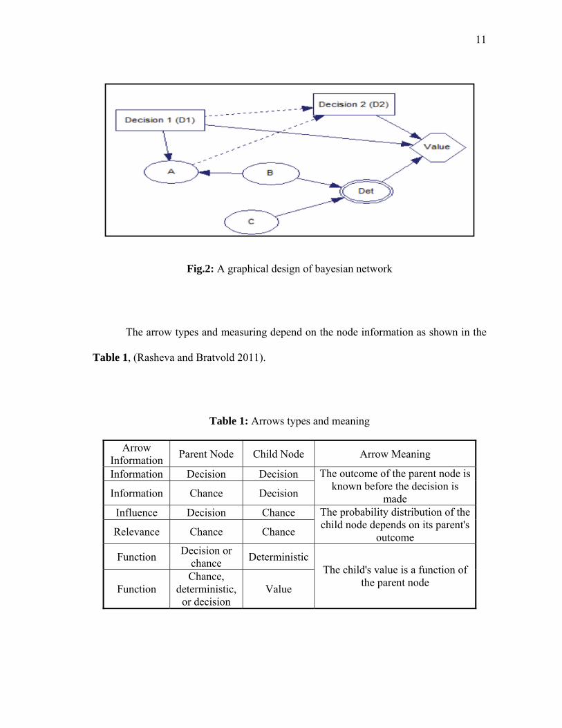
Expert opinions and real-time data were used to construct Bayesian Network for

optimal placement of horizontal wells. The well placement decision making process

requires opinions from different backgrounds. Bayesian Network was used to design,

evaluate and support real time drilling processes. The graphical design shows joint

probability distribution in decisions, uncertainties, and values. A decision node is shown

as rectangle and a chance node as oval. The value node is shown as hexagons as shown

in Fig.2, (Rasheva and Bratvold 2011).

11

Fig.2: A graphical design of bayesian network

The arrow types and measuring depend on the node information as shown in the

Table 1, (Rasheva and Bratvold 2011).

Table 1: Arrows types and meaning

Arrow Information Parent Node Child Node Arrow Meaning

Information Decision Decision The outcome of the parent node is known before the decision is

made Information Chance Decision

Influence Decision Chance The probability distribution of the child node depends on its parent's

outcome Relevance Chance Chance

Function Decision or chance Deterministic

The child's value is a function of the parent node Function

Chance, deterministic,

or decision Value

12

Bayesian Network was used to aid in setting casing depth in North Sea.

Probabilities can be extracted from data or simulation outputs or be elicited (from

subject experts). Elicited probabilities should have reflective accuracy. The derived

distribution should represent expert’s knowledge. For the probability distributions of the

nodes, first the unconditional marginal probability distribution of root nodes (without

parents) is assigned by the experts. After that, the conditional probability distribution for

each node is assigned. These assigned values can be continuous or discrete, Fig.3,

(Rajaieyamchee and Bratvold 2009).

Fig.3: Assigning conditional probabilities distribution for each node

13

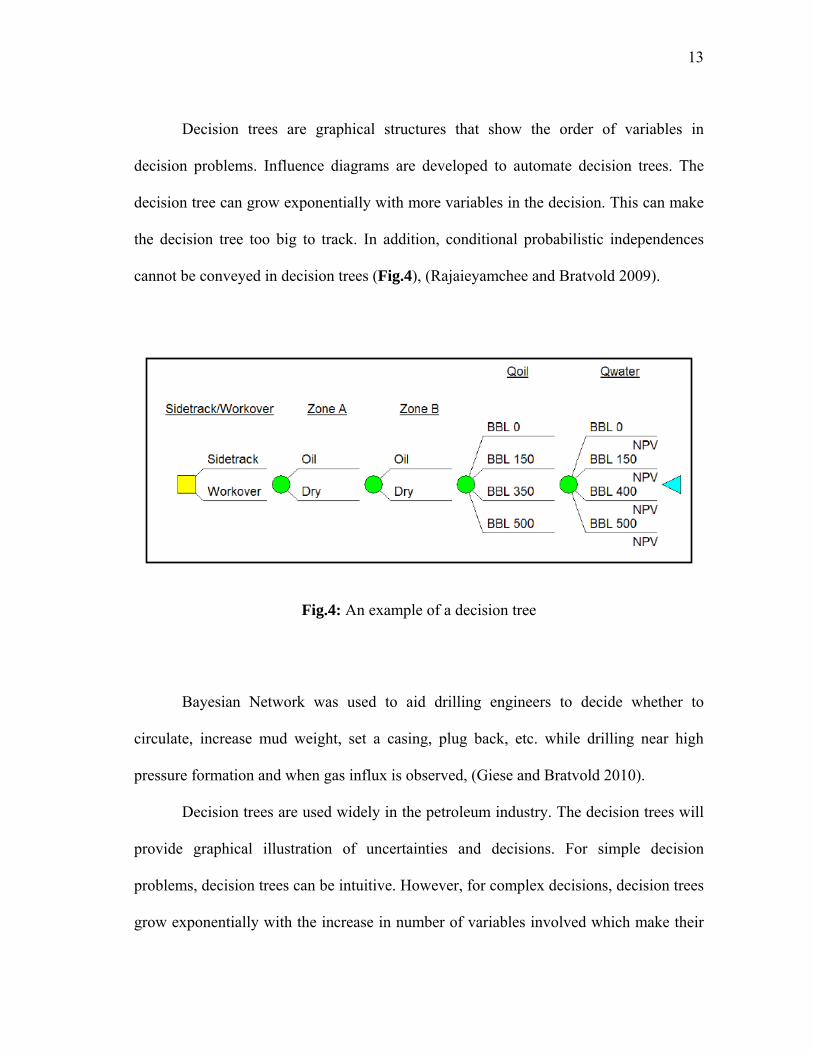
Decision trees are graphical structures that show the order of variables in

decision problems. Influence diagrams are developed to automate decision trees. The

decision tree can grow exponentially with more variables in the decision. This can make

the decision tree too big to track. In addition, conditional probabilistic independences

cannot be conveyed in decision trees (Fig.4), (Rajaieyamchee and Bratvold 2009).

Fig.4: An example of a decision tree

Bayesian Network was used to aid drilling engineers to decide whether to

circulate, increase mud weight, set a casing, plug back, etc. while drilling near high

pressure formation and when gas influx is observed, (Giese and Bratvold 2010).

Decision trees are used widely in the petroleum industry. The decision trees will

provide graphical illustration of uncertainties and decisions. For simple decision

problems, decision trees can be intuitive. However, for complex decisions, decision trees

grow exponentially with the increase in number of variables involved which make their

14

use impractical. Bayesian Network can be used when dealing with complex decision

problems easily compared to decision trees, (Giese and Bratvold 2010).

Wright (1921, 1934) and Good (1961a, b) used graphical structure for illustrating

joint probability distributions. (Howard and Matheson 1981) explained this illustration in

more details. (Kim and Pearl 1983), (Lauritzen and Spiegelthaler 1988) and Pearl (1988)

have introduced computer science and statistics into the graphical representation of joint

probability distributions.

A simple problem example is shown in Fig.5. The following observation can

explain the model, (Giese and Bratvold 2010):

• There is pore pressure that depends on depth and well geology,

• Measurement of depth is shown in the model,

• Equivalent circulating density (ECD) downhole is also shown and can be

estimated using flow and mud weight,

• Gas will flow into the wellbore if the pore pressure is greater than ECD.

Fig.5: A simple problem example

15

Expert system based on Bayesian Network was used for selection of proper EOR

techniques. The expert system was applied to 10 Iranian southwest reservoirs. CO2

flooding showed to be the most practical method for EOR in these 10 wells, Zerafat et

al. (2011).

A Bayesian Network can behave similarly to human begins when dealing with

uncertainties to predict the likelihood of future operations from given prior trials.

Subjectivity is a limitation of Bayesian method when handling prior belief, Zerafat et al.

(2011).

Bayesian Network was performed to assess the risk from nuclear waste disposal,

Lee et al. (2005). Bayesian Network was also used to model flow to select the model

with greatest uncertainty at the boundaries, Abbaspour et al. (2000). Hydrodynamic

behavior characterization was also done by Bayesian Network, Ferraresi et al. (1996).

Most probable areas of salinity sources distribution in the Gaza aquifer were done using

Bayesian Network, Ghabayen et al. (2006).

Existing systems cannot deal with certain geotechnical risks for example

excessive deformation or rock falls. The reason behind that is the need to capture expert

knowledge. To achieve this, Bayesian Network was used to model these uncertainties.

Using fault tree analysis for encoding uncertain expert knowledge can result in

significant complications, (Sousa and Einstein 2007).

Bayesian Network was used for pipeline leak detection. Prior probabilities were

integrated to detect leaks, Carpenter et al. (2003). Bayesian network was used to design

models to support geosteering decisions. Using Bayesian Network can lead to reduction

16

of required number of operators on rig sites. Previous systems were built using fuzzy

logic and neural networks, Lloyed et al. (1990), Dashevski et al. (1999), and Stoner

(2003). The limitations of these approaches are:

• The knowledge database and inference algorithms are inseparable. Thus

adding new rules or changes require programming again. This makes

updating the expert system difficult and challenging.

• The previous approaches are limited in their ability to make decisions under

uncertainty.

Bayesian Network was used to analyze and support geosteering decisions.

Drillers’ opinions were considered under conditions of uncertainty. Drillers were also

able to update the model with the arrival of new data, (Rajaieyamchee and Bratvold

2010).

Decisions must be made without elimination of uncertainty. The use of Bayesian

Network supported the real time decision making. The reason behind this is the ability to

update the probabilistic information embedded in the network with new data arrival,

Fjellheim et al. (2011).

The objective of this research is to propose models to serve as training tools or a

guide to aid drilling engineers and scientists in field operations in five areas:

1. Cementing Operations

2. Completion Operations

3. Drilling Fluids Operations

4. Underbalanced Drilling Operations

17

5. Well Control Operations

In order to prove the concept and the benefits of using this approach, one simple

BDN model simulating the decision-making process of the selection of swelling packer

is introduced in Chapter II.

18

CHAPTER II

MODEL FOR THE PROOF OF THE CONCEPT*

In order to prove the concept and the benefits of using this approach, one simple BDN

model simulating the decision-making process of the selection of swelling packer is

introduced in Fig.6. This model contains one decision node (swelling packer), three

uncertainty nodes (treating fluid, type of drilling fluid, and Consequences), and one

value node (Completion Expert System).

Fig.6: BDN model for the proof of the concept

____________ *Reprinted with permission from “Expert System for the Optimal Design and Execution of Successful Completion Practices Using Artificial Bayesian Intelligence,” by Al-Yami, A.S., Schubert, J., and Beck, G., 2011, SPE 143826, Copyright © 2012, Society of Petroleum Engineers.

19

In this model, our selections for swelling packers are affected by our selection of

treating fluid and drilling fluids. Once the structure of the BDN is defined, it is required

to define the probability states associated with each node. These are given in Table 2

through Table 6. The model is designed in a way that the engineer will select his

uncertainty nodes (treating fluid and/or type of drilling fluid) to select the recommended

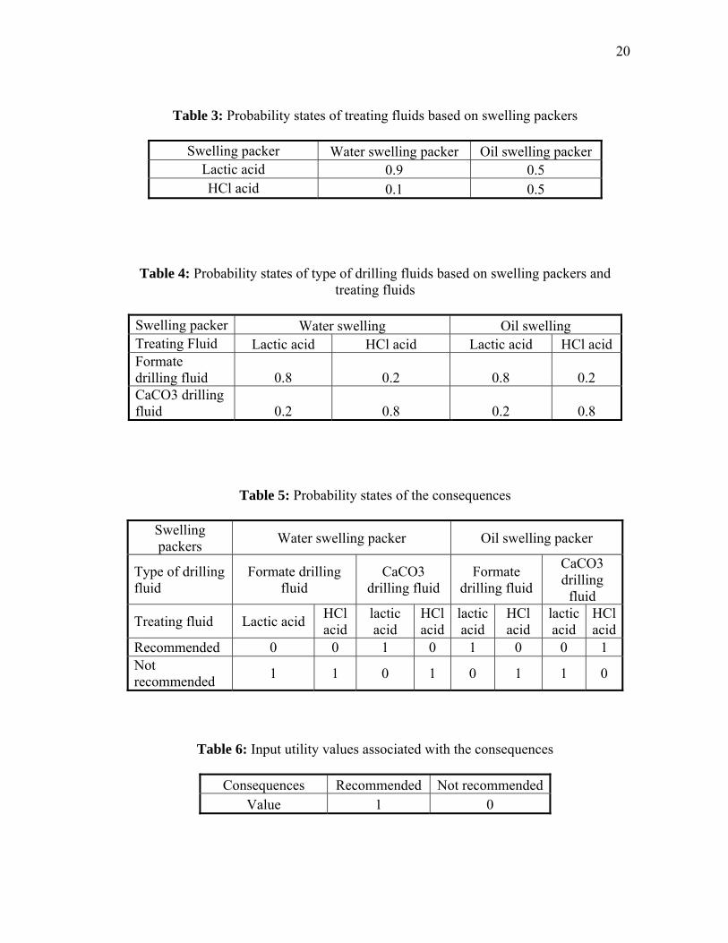
type of swelling packer (oil swelling or water swelling packer, Table 2). Table 3 shows

the probability states of treating fluids based on swelling packers. Lactic acid has a

probability of 0.9 for success when using water swelling packers but only 0.1 chance of

success when using lactic acid. Table 4 shows the probability states of type of drilling

fluids based on swelling packers and treating fluids. Table 5 defines the extent of the

probability states of the consequences, which are defined as recommended and not

recommended. The input utility value associated with the consequences is given in

Table 6. The expected utility outcomes considering all possible cases of evidence set a

minimum value of zero, which is the “not recommended” case, and a maximum value of

one, which assumed to be the “recommended” case.

Table 2: Swelling packers

Water swelling packer Oil swelling packer

20

Table 3: Probability states of treating fluids based on swelling packers

Swelling packer Water swelling packer Oil swelling packer Lactic acid 0.9 0.5 HCl acid 0.1 0.5

Table 4: Probability states of type of drilling fluids based on swelling packers and

treating fluids

Swelling packer Water swelling Oil swelling Treating Fluid Lactic acid HCl acid Lactic acid HCl acid Formate drilling fluid 0.8 0.2 0.8 0.2 CaCO3 drilling fluid 0.2 0.8 0.2 0.8

Table 5: Probability states of the consequences

Swelling packers Water swelling packer Oil swelling packer

Type of drilling fluid

Formate drilling fluid

CaCO3 drilling fluid

Formate drilling fluid

CaCO3 drilling

fluid

Treating fluid Lactic acid HCl acid

lactic acid

HCl acid

lactic acid

HCl acid

lactic acid

HCl acid

Recommended 0 0 1 0 1 0 0 1 Not recommended 1 1 0 1 0 1 1 0

Table 6: Input utility values associated with the consequences

Consequences Recommended Not recommended Value 1 0

21

The main goal after the required inputs are entered into the model is to simulate

the uncertainty propagation from the existing sources of evidence, which means moving

the information forward starting from the swelling packers node. First the total

probability is calculated for the type of drilling fluid. The above model shows that our

selection of drilling fluid will affect the treating fluid and our swelling packers.

The below equation is used:

The results are shown in Table 7. Tables 3&4 are used for this calculation for

example:

Table 7: Total probability for type of drilling fluid

Swelling packer Water swelling packer

Oil swelling packer

Formate drilling fluid 0.74 0.5

CaCO3 drilling fluid 0.26 0.5

Then Bayesian equation can be used as shown below:

)()(1

i

m

ii

APABP∑=

( ) ( ) 74.02.01.08.09.0)()(1

=×+×=∑=

acidlacticPacidlacticfluiddrillingformatePm

ii

⎟⎟⎠

⎞⎜⎜⎝

⎛=

)()()(

)(evidencep

hypothesisphypothesisevidencepevidencehypothesisp

22

Which is the same thing as:

The results are shown in Table 8. Tables 3, 4 and 7 are used for this calculation.

The calculation shows the probabilities of selecting treating fluids (lactic acid or HCl

acid) when the engineer wants to use a certain drilling fluid (formate or CaCO3) for a

particular swelling packer (oil or water swelling). The detailed calculations for water

swelling packer are shown below:

For oil swelling packer, the calculations are:

9729.074.0

9.08.0)(

)()()( =

×=⎟⎟⎠

⎞⎜⎜⎝

⎛=

formatepacidlacticpacidlacticformatep

formateacidlacticp

0270.074.0

1.02.0)(

)()()( =

×=⎟⎟⎠

⎞⎜⎜⎝

⎛=

formatepacidHClpacidHClformatep

formateacidHClp

6923.026.0

9.02.0)(

)()()(

3

33 =

×=⎟⎟⎠

⎞⎜⎜⎝

⎛=

CaCOpacidlacticpacidlacticCaCOp

CaCOacidlacticp

3076.026.0

1.08.0)(

)()()(

3

33 =

×=⎟⎟⎠

⎞⎜⎜⎝

⎛=

CaCOpacidHClpacidHClCaCOp

CaCOacidHClp

8.05.0

5.08.0)(

)()()( =

×=⎟⎟⎠

⎞⎜⎜⎝

⎛=

formatepacidlacticpacidlacticformatep

formateacidlacticp

2.05.0

5.02.0)(

)()()( =

×=⎟⎟⎠

⎞⎜⎜⎝

⎛=

formatepacidHClpacidHClformatep

formateacidHClp

8.05.0

5.08.0)(

)()()(

3

33 =

×=⎟⎟⎠

⎞⎜⎜⎝

⎛=

CaCOpacidlacticpacidlacticCaCOp

CaCOacidlacticp

23

Table 8: Using bayesian equation for the proposed model

Swelling packer Water swelling Oil swelling

Treating Fluid Updated values Updated values Lactic acid 0.9729 0.6923 0.8 0.2 HCl acid 0.027 0.3076 0.2 0.8 Type of

drilling fluid Updated values Updated values

Formate drilling fluid

Selected by user Selected by user

CaCO3 drilling fluid Selected by user Selected

by user Now, once the Bayesian calculations are completed, there are two approaches for

the engineers to use this model. The first approach is to specify the type of drilling fluid

he wants to use to drill the well and this will determine the correct decision in this model

which is the suitable swelling packer. For example if CaCO3 is required to drill the well,

then the probabilities of using the packers (consequences) in Table 8 and probability

states of the consequences in Table 5 are used. The results are shown in Table 9. Below

is an example calculation when CaCO3 drilling fluid is selected:

Water swelling packers

Oil swelling packers

2.05.0

5.02.0)(

)()()(

3

33 =

×=⎟⎟⎠

⎞⎜⎜⎝

⎛=

CaCOpacidHClpacidHClCaCOp

CaCOacidHClp

3076.0)3076.0106923.0(Re

6923.0)3076.006923.01(Re

=×+×

=×+×commendedNot

commended

24

Table 9: Consequences when selecting CaCO3 drilling fluid (from table 7) and table 4

Swelling Packers Water swelling packers Oil swelling packers Recommended 0.6923 0.8

Not recommended 0.3076 0.2

The utility in Table 10 is finally calculated using below equation from Table 9

and Table 6:

For water swelling packer it is:

For oil swelling packer it is:

Table 10: Expected utility values (first approach)

Swelling packer Water swelling Oil swelling Expected utility 0.6923 0.8

The other option for the engineer to use this model is to specify all the

uncertainties (drilling fluid and treating fluid) to determine the optimum selection of

6923.003076.016923.0 =×+×=×= ∑i

believeinputresultceconsequenutilityExpected

8.002.018.0 =×+×=×= ∑i

believeinputresultceconsequenutilityExpected

2.0)8.0012.0(Re

8.0)0.18.002.0(Re

=×+×

=×+×commendedNot

commended

25

swelling packers. Table 5 can be used directly. For example selecting formate drilling

fluid and lactic acid indicate that oil swelling packer is recommended, Table 11.

Table 11: Consequences when selecting formate drilling fluid and lactic acid (from table

5)

Swelling Packers Water swelling packers Oil swelling packers

Recommended 0 1 Not recommended 1 0

The utility is calculated as mentioned above, Table 12.

Table 12: Expected utility values (2nd approach)

Swelling packer water swelling oil swelling Expected utility 0 1

For this study, Graphical Network Interface was used for calculations of the

uncertainty propagation to build up the expert system. Fig.7 shows the results for the

first approach example (selecting CaCO3 drilling fluid) which agrees with the calculation

above. Fig.8 shows the results for the second approach example (selecting formate

drilling fluid and lactic acid treating fluid) which also agrees with the calculation above.

26

Fig.7: Model for the proof of concept (first approach)

Fig.8: Model for the proof of concept (second approach)

27

Using Bayesian Intelligence allows the design of drilling and completion expert

systems that can be used in different fields and/or by different experts with different

opinions. The system can be updated easily with the new opinions by changing the

probability states shown above (Tables 3-5) and the model will update the calculation to

show the recommended type of swelling packer.

28

CHAPTER III

WELL COMPLETION EXPERT SYSTEM*

The objective of this chapter is to propose a set of guidelines for the optimal completion

design, by integrating current best practices through a decision-making system based on

Artificial Bayesian Intelligence. Best completion practices collected from data, models,

and experts' opinions, are integrated into a Bayesian Network BN to simulate likely

scenarios of its use, that will honor efficient designs when dictated by varying well

objectives, well types, temperatures, pressures, rock and fluid properties.

The described decision-making model follows a causal and uncertainty-based

approach capable of simulating realistic conditions on the use of completion operations.

For instance, the use of water swelling packer dictates the use of organic acids instead of

HCl acids. However, rock type and well geometry affect our selection of treatment

fluids. Another example is selection of sand control method based on rock properties.

The chapter also outlines best operational practices in fracturing, sand control,

perforation, treatment and completion fluids, multilateral junction level selection and

lateral completion. Completion experts' opinions were considered in building the model

in this paper.

____________ *Reprinted with permission from “Expert System for the Optimal Design and Execution of Successful Completion Practices Using Artificial Bayesian Intelligence,” by Al-Yami, A.S., Schubert, J., and Beck, G., 2011, SPE 143826, Copyright © 2012, Society of Petroleum Engineers.

29

Fig.9 shows the completion expert model. Literature review and completion

experts’ opinions were used as evidence to build the model using the proposed Bayesian

Network. Variable nodes allow the user to input desired well conditions that allows for

generating the corresponding best completion practices. Eighteen uncertainty nodes are

defined for this model to determine best practices in six decision nodes. The model is

divided into six parts or decisions. Each decision has uncertainties and consequences

nodes. The consequences node combines the uncertainty nodes where completion expert

opinions were used to assign and define the conditional probability distribution. The

model then calculates the optimum practices decision. Below are descriptions of each

decision in the model.

3.1 Junction classification decision

The uncertainty node is named considerations in designing multilateral junctions. Table

13 shows its probability states. There are six levels in TAML classification as detailed

below:

• Level 1: open unsupported junction.

• Level 2: Motherbore cased and cemented and lateral open.

• Level 3: Motherbore cased and cemented and lateral cased but not cemented.

• Level 4: Motherbore and lateral cased and cemented.

• Level 5: Pressure integrity is provided at the junction using straddle packers.

• Level 6: Pressure integrity is provided using integral mechanical seal that can

include reformable junction or non-reformable and full diameter splitter.

30

Fig.9: Completion expert model

31

Table 13: Probability states of considerations in designing multilateral junctions’ node

Consolidated strong formation and zonal control is not critical 0.15 Formation stability is required but not at the junction 0.15 Formation stability is required and mechanical isolation and limited stability at the junction 0.15

Re entry is possible 0.15 Formation stability is required and hydraulic isolation and stability at the junction 0.15

best completion for weak incompetent susceptible to wellbore collapse 0.05 single component completion hydraulic isolation is maximum and does not depend on cementing and continuous liner ID accessing both bores increase well control capability

0.05

kickoff point is not possible at strong formation 0.15 The decision node has six options, Table 14. Fig. 10 shows part of the

consequences. For consolidated strong formation where zonal control is not required,

level 1 is the optimum design. When formation stability is required but not at the

junction then level 2 is the optimum practice. As mentioned above, different experts can

update these numbers easily in case they do not agree with them.

Table 14: Junction classification decision node

Level 1Level 2Level 3Level 4Level 5Level 6

32

Fig.10: Part of consequences for junction classification selection

3.2 Treatment fluid

For the treatment fluid decision, there are two uncertainties (factors). The first one is the

well type (short or long lateral), Table 15. The second uncertainty node is the type of

drilling fluid used, Table 16. The treatment fluid decision is shown in Table 17. Fig. 11

shows part of the consequences input. In case of long horizontal lateral and when using

CaCO3 drilling fluid, the optimum practice is either to use lactic acid or formic acid.

Table 15: Probability states of well type node

short horizontal section 0.5

Long horizontal section 0.5

Table 16: Probability states of type of drilling fluid node

Water based mud with CaCO3 0.2 Water based mud with Barite 0.2 Emulsion oil based mud 0.2 All oil based mud 0.2 Potassium formate mud 0.1 Drilling fluid based with Mn3O4 0.1

33

Table 17: Treatment fluids decision node

Inhibitors Amines Alcohol methanol Acid less than 15 wt percentage HCl acid Acid more than 15 wt percentage HCl acid HF acid less than 65 wt percentage Acetic acid Surfactants Citric Formic Lactic Potassium formate Enzymes Circulation of new volume of drilling fluid

Fig.11: Part of consequences for completion (treatment) fluid selection

3.3 Lateral completion

The lateral completion decision has four uncertainties (cost, zonal isolation, reliability

and productivity). Each one of them has three levels (high, medium and low). There is

also an additional uncertainty which is potential of sand production. In the model we can

see that our selection of junction classification decision affect the potential of sand

production uncertainty. As known, level 1 and 2 do not have sand production potential.

The lateral completion is shown in Table 18. Fig. 12 shows that for a formation that has

34

sand production problem, and for good reliability, good productivity, good cost and good

zonal isolation, the optimum practice is to use openhole expandable screen.

Table 18: Lateral completion decision node

Standalone screen Open hole gravel pack Cased hole gravel pack Frac pack Openhole expandable screens

Fig.12: Part of consequences for completion selection

3.4 Perforating

The perforating part of the model outlines the decision into more steps compared to the

other parts. The user will need to determine if underbalanced perforation is useful or not

(Table 19) which will affect the decision of formulating non damaging fluids or

temperature consideration, Table 20. Tables 21 and 22 give probability states that lead

to detailed analysis that goes to the consequences node. Part of the consequences input,

35

Fig. 13, shows that if we can formulate non-damaging fluid then the optimum practice is

to design for overbalanced perforation using wire line conveyed casing guns. The

perforating decision node details are shown in Table 23.

Table 19: Probability states of if UB perforation useful or not

Completion Standalone screen

Openhole gravel pack

Cased hole

gravel pack

Frack pack

Openhole expandable

screen

Not required 1 1 0 1 1

Yes 0 0 0.5 0 0 Not 0 0 0.5 0 0

Table 20: Probability states of fluid damage and temperature effect

Is Underbalanced perforation useful Yes No can we formulate non damaging fluid 0.2 0.8 Need to consider temperature 0.8 0.2

Table 21: Probability states of consideration factors

Fluid damage and temperature effect

can we formulate non damaging fluid

Need to consider temperature

Higher than 450 °F 0.1 0.4 Lower than 450 °F 0.1 0.4 We can formulate non damaging fluid 0.4 0.1

We cannot formulate non damaging fluid 0.4 0.1

36

Table 22: Probability states of detailed analysis

Consideration factors Higher than 450 F

Lower than

450 F

We can formulate

Non-damaging

fluid

we cannot formulate

non-damaging fluid

multiple runs with through tubing guns cannot achieve adequate well rates

0.25 0.1 0.1 0.1

multiple runs with through tubing guns can achieve adequate well rates

0.25 0.1 0.1 0.1

through tubing guns can be used 0.1 0.25 0.1 0.1

through tubing guns cannot be used 0.1 0.25 0.1 0.1

can the damage be removed by acidizing in carbonate formation

0.1 0.1 0.1 0.25

can the damage be removed by fractured stimulation

0.1 0.1 0.1 0.25

we can formulate non damaging fluid 0.1 0.1 0.4 0.1

Table 23: Perforating decision node

Multiple runs with through tubing guns through tubing guns Design for tubing conveyed perforation Consider if underbalanced perforating with casing guns is acceptable and evaluate fluid damage risks during completion running if well will kill itself if perforated without tubing Consider perforating overbalanced in acid with casing or through tubing guns Review special perforation requirements for fracturing such as diversion and proppant placement Design for overbalanced perforating using wire line conveyed casing guns

37

Fig.13: Part of consequences for perforation selection

3.5 Openhole gravel packing

The openhole gravel packing section shows two types of gravel packing methods

(alternate path and circulating pack). The circulating pack is more suitable where there is

no fluid loss while alternate path is applied when there is a potential for lost circulation

as shown in the probability states in Tables 24 and 25. Table 26 shows the probability

states for designing details such as slurry density and applied pressure. Table 27 shows

the openhole gravel packing decision details for the treatment. Part of the consequences

is shown in Fig. 14 where it shows that it is possible to exceed the fracturing pressure

when following the alternate path.

Table 24: Probability states of potential fluid loss formation

Completion Standalone screen

Openhole gravel pack

Cased hole gravel pack

Frack pack

Openhole expandable

screen Not required 1 0 1 1 1

Fluid loss 0 0.5 0 0 0 No fluid loss 0 0.5 0 0 0

38

Table 25: Probability states of type of openhole gravel packing

Potential fluid loss formation

Fluid loss No fluid loss

Alternate path 1 0 Circulating pack 0 1

Table 26: Probability states designing details

gravel pack fluids 0.1 slurry density 0.1 Fluid volume and time 0.1 Fluid loss 0.2 Pressure 0.1 Hole condition 0.1 Filter cake removal 0.1 Screen size 0.1 Cost 0.1

39

Table 27: Openhole gravel packing decision node

gravel pack fluid of water or oil with viscosifier gravel pack fluid of water used with friction reducer high slurry density of 8 ppa low slurry density of up to 2 ppa low fluid volume and reduced pumping time large fluid volume No need for complete returns Complete returns is required can exceed fracture pressure cannot exceed fracture pressure critical washout is not a problem critical washout is a problem filter cake need to be removed filter cake does not have to be removed small base pipe but larger overall diameter for shunts large base pipe screen less time but more expensive chemicals More rig time for pumping is required

Fig.14: Part of consequences for openhole gravel pack selection

40

3.6 Packer selection

The packer model part indicates that selection of packers depends on completion fluids

(Table 28), oil and gas details (Table 29), wellbore fluids (Table 30), and treatment

fluids (Table 17). For example water swelling packers are damaged by CaCl2 brines and

HCl acids. Table 31 shows the available packers for the user to select. Fig. 15 shows

part of the consequences for the optimum conditions for the PVDF Coflon packer

applications.

Table 28: Probability states of completion fluids node

CaCl2/CaBr 0.25ZnBr 0.25K2CO3 0.25Brine seawater 0.25

Table 29: Probability states of oil and gas node

Aliphatic hydrocarbons 0.1Aromatic hydrocarbons 0.1Crude oil less than 250 °F 0.2Crude oil more than 250 °F 0.2Sour crude 0.2Gas sour natural gas 0.2

41

Table 30: Probability states of wellbore fluids node

water 0.2 steam 0.2 methane 0.2 CO2 0.2 H2S 0.2

Table 31: Packer selection decision node

CR Neoprene AE AU Urethane

NBR Nitrile ECO Hydrin PVDF Coflon

HNBR Therban FKM Viton ETFE Tefzel FCM Aflas

PEEK Victrex FFKM Kalrez PTFE Teflon

Oil swelling packer water swelling packer

Fig.15: Part of consequences for packer selection

42

3.7 Final consequences

All different parts of the big model consequences are gathered into one node named final

consequences. The final consequences is used to select optimum practices from the

whole model ( all decision nodes i.e. lateral junction, treating fluids, lateral completion,

perforation, gravel packing, and packer selection). Fig. 16 shows part of the final

consequences. A value of 1 is assigned to the recommended practices from each decision

node in the model.

Fig.16: Part of consequences for the final consequences node

3.8 Completion expert system utility node

In the model, there is only one utility node to calculate the expected values from the final

consequences node, Table 32.

Table 32: Expected utility values for the final consequences node

Final Consequences Recommended Not

recommended Value 1 0

43

CHAPTER IV

DRILLING FLUIDS MODEL*

Drilling fluids are important factor in drilling and completion operations. Designing

drilling fluids depend on formation lithology, temperature and pressure. The objective of

this chapter is to set a module that should aid drilling engineers when designing drilling

fluids. A module was created based on several inputs. To create this module, we

interviewed experts to gather the information required to determine best practices as a

function of different probabilities. Drilling fluids formulations were gathered from Saudi

Arabia fields to build up this model.

Fig.17 shows the drilling fluids model. Literature review and drilling fluids

experts’ opinions were used as evidence to build a model using the proposed Bayesian

Network.

Variable nodes allow the user to input desired well conditions that allows for

generating the corresponding best drilling fluids practices. Three uncertainty nodes are

defined for this model to determine best practices in one decision node (recommended

drilling fluids).

____________

*Reprinted with permission from “Drilling Fluids Consultation System: Development and Field Applications,” by Al-Yami, A.S. and Schubert, J., 2012a, SPE 152098, Copyright © 2012, Society of Petroleum Engineers.

44

The model has one decision which has uncertainties and one consequence node. The

consequence node combines the uncertainty nodes where drilling fluids’ expert opinions

were used to assign and define the conditional probability distribution. The model then

calculates the recommended drilling fluids decision.

Fig.17: Overall model of drilling fluids expert system

The first uncertainty node is the temperature range, Fig.18. Temperature is

divided into 4 ranges since different polymers used in drilling fluids are affected by

temperature.

45

Fig.18: Temperature options

The second node is the potential hole problems uncertainty, Fig. 19. These

problems are considered to be general problems that need to be considered when

designing drilling fluids. The consequences node depends on the temperature range and

potential hole problems probabilities selected.

46

Fig.19: A list of potential hole problems

The last uncertainty node in the model is the Saudi Arabia formation, Fig.20. The

objective of this node was to use this model in Saudi Arabia fields.

47

Fig.20: Formations’ names in Saudi Arabia

48

CHAPTER V

WELL CONTROL MODEL*

The objective of this chapter is to propose a set of guidelines for optimal well control

operations, by integrating current best practices through a decision-making system based

on Artificial Bayesian Intelligence.

The proposed decision-making model follows a causal and an uncertainty-based

approach capable of simulating realistic conditions on the use of well control operations.

For instance, as the user varies the operation, rig and crew capabilities, kick details (such

as slim hole, deviated or horizontal well), the system will show the optimum practices

for circulation method.

The advantage of the Artificial Bayesian Intelligence method is that it can be

updated easily when dealing with different opinions. The outcome of this paper is user-

friendly software, where you can easily find the specific subject of interest, and by the

click of a button, get the related information you are seeking. The model is divided into

three parts or decisions. Each decision has uncertainties and consequences nodes. The

consequences node combines the uncertainty nodes where well control expert opinions

were used to assign and define the conditional probability distribution. The model then

calculates the optimum practices decision.

____________

*Reprinted with permission from “Development of Optimum Well Control Practices Using Artificial Bayesian Intelligence,” by Al-Yami, A.S. and Schubert, J., 2012c, OTC 22882, Copyright © 2012, Society of Petroleum Engineers.

49

Fig.21 shows the model which is divided into three parts of uncertainty and

decision nodes. The first provides the proposed circulation method decision based on the

kick details provided. The second part provides the user the optimum recommended

practice based on the possible scenarios and operations in well control. The third part

provides the user with a quick check list for trouble shooting in case of problems while

controlling the well.

Fig.21: Well control expert model

Kick indicators’ uncertainties are shown in Fig.22. The kick can be verified by

checking the flow when pumps are off, Fig. 23.

50

Fig.22: Kick indicators

Fig.23: Verification

51

The kick details’ uncertainty (Fig.24) affects the user selection of proposed

circulation methods shown in Fig.25.

Fig.24: Possible kick details

Fig.25: Proposed circulation method

52

Experts’ opinions were used to build up the node known as consequences for

optimum method of circulation method, Fig.26 by assigning 1 to the optimum

circulation method. This node can be updated easily when different opinions are

presented.

Fig.26: Part of consequences for optimum method of circulation method

The second part is related to proper well control practices under different

scenarios such as driller method, killing deep wells, etc as shown in Fig.27. A long list

of possible operations (probabilities) was assigned to the possible operation node as

shown partially in Fig.28.

53

Fig.27: Possible scenarios in well control

Fig.28: Part of possible operations

54

The recommended practice probabilities for proper well control are shown in

Fig.29. Experts’ opinions were used to assign probability values in the consequence of

proper well control practices. Part of the assigned values is shown in Fig.30. Again these

probabilities can be updated easily by different experts or at different field conditions.

Fig.29: A list of recommended practices

Fig.30: Part of consequences of proper well control practices

55

The third part is designed to assist the user to find the optimum solution for a list

of potential problems that can be faced during well control operations. A check list of

trouble shooting is shown in Fig.31. The model also recommends a list of actions and

observes their results by using the action and results node. This node is affected by the

user selection from the check list for trouble shooting node. Part of actions and results

are shown in Fig.32.

Fig.31: Check list for possible trouble shooting

56

Fig.32: A list of possible actions and results

Based on the user selection of action taken and result node the problem can be

identified. A list of problem probabilities is shown in Fig.33. Finally, once the problem

is identified, an optimum solution from the solution decision can be recommended. Part

of the solution is shown in Fig.34. Experts’ opinions are used to assign probability

values to the consequences of trouble shooting node. Part of these values is shown in

Fig.35.

57

Fig.33: A list of possible problems

Fig.34: Part of possible solutions

58

Fig.35: Part of consequences of trouble shooting

The user can select which part he needs individually or can use all parts together

at the same time by selecting probability values from desired uncertainty nodes. The

final sequence will select the optimum practice from each consequence (optimum

method of circulation method consequence, trouble shooting guide consequence and

consequence of proper well control practice); part of the final consequence is shown in

Fig.36.

Fig.36: Final consequences

59

CHAPTER VI

CEMENTING MODEL*

Cementing is an important factor in drilling and completion operations. Good cementing

practices are required for a proper advancing in drilling and production operations.

Successful cementing practices start with the design of effective cement slurries.

The objective of this chapter is to propose a set of guidelines for the optimal

design of cement slurries, by integrating current best practices through a decision-

making system based on Artificial Bayesian Intelligence. Best cementing practices

collected from Saudi Arabia fields are integrated into a Bayesian Network BN to

simulate likely scenarios of its use, which will honor efficient designs when dictated by

varying well objectives, well types, temperatures, pressures, and drilling fluids.

The proposed decision-making model follows a causal and an uncertainty-based

approach capable of simulating realistic conditions on the use of cement slurries during

drilling and completion operations. For instance, well sections and drilling operations

dictate the use of the proper cement design, which may include the use of specific

additives according to the particular modeling scenarios.

____________

*Reprinted with permission from “Drilling Expert System for the Optimal Design and Execution of Successful Cementing Practices,” by Al-Yami, A.S., Schubert, J., Medina, C., and Ok-Youn, Y., 2010b, IADC/SPE 135183, Copyright © 2010, Society of Petroleum Engineers

60

These include operations on surface casing, top jobs, intermediate casings, cementing in

weak formations, squeeze treatment, kickoff and isolation plugs, horizontal, and vertical

completions, among others.

Fig.37. shows the cementing expert model. Six uncertainty nodes are defined for

this model (well type, objectives, bottom hole static temperature, pumping time, drilling

fluids, and consequences). This considers three decision criteria. The three decisions are

a) recommended cementing formulations, b) recommended spacers formulations and c)

recommended operational practices.

The uncertainty node corresponding to the well type enables the drilling engineer

to set his/her evidence (i.e. to select his well type) as oil well, or gas well. The bottom

hole static temperature uncertainty node enables the selection of the temperature range.

Temperature ranges were selected for oil and gas wells up to 400 °F. Bottom hole static

temperature affects required pumping time. The user can either select a temperature or a

suitable pumping time for the proposed well section. Pumping time ranges up to 8 hours

in this model.

The Objective uncertainty node enables the user to select the objective of the

operation. Different options are made available for the user. These include kickoff and

isolation plugs; squeeze cementing, single stage cementing, conductor, surface,

intermediate and production casings. In addition, the objective uncertainty node has

cementing long liners, expandable casings, and cementing CO2 injection wells. The

Drilling Fluid Type uncertainty node shows possible options such as water based, water

61

based with high Cl- content, and oil based mud. The drilling fluid type mainly affects the

spacer selection.

The recommended cement formulations decision node contains all possible

cementing slurries that correspond to the different well type, objective nodes and bottom

hole temperature. The recommended spacer decision node shows all possible spacer

formulations (water, water based fluid, special spacer fluid with mutual solvent and

water wetting additives). The recommended operational practices decision node shows

required actions for each casing type such as multistage operation, optimum pump rate,

surface shallow leaks and other best practices related to cementing such as top jobs and

cementing plugs recommendations.

The consequences node combines the four uncertainty nodes (well type, required

pumping time, objective and drilling fluid) and the three decision nodes (recommended

cement formulations, recommended spacers and recommended operational practices).

Cementing experts’ opinions were used to assign and define the node conditional

probability distribution.

The model is designed in a way to give the user options to design well cementing

and best practices effectively. The user will select options that match his application

from well type, bottom hole temperature or required pumping time, objective and

drilling fluid. Then the model (cementing expert utility) will suggest optimum cement

formulations, spacer formulations and operational practices that fit the given well

conditions.

62

Fig.37: Cementing expert model based on bayesian network

63

CHAPTER VII

UNDERBALANCED DRILLING MODELS*

The objective of this chapter is to propose a set of guidelines for the optimal

underbalanced drilling operations, by integrating current best practices through a

decision-making system based on Artificial Bayesian Intelligence.

The outcome of this chapter is user-friendly software, where you can easily find

the specific subject of interest, and by the click of a button, get the related information

you are seeking. Literature review and experts’ opinions were used as evidence to build

these models using the proposed Bayesian Network. Variable nodes allow the user to

input desired conditions that allows for generating the corresponding best practices.

Underbalanced drilling expert system here is combined into nine models as follow:

• General approach to underbalanced drilling

• Flow underbalanced drilling

• Gaseated underbalanced drilling

• Foam underbalanced drilling

• Air and gas underbalanced drilling

____________

*Reprinted with permission from “Guidelines for Optimum Underbalanced Drilling Practices Using Artificial Bayesian Intelligence,” by Al-Yami, A.S. and Schubert, J., 2012d, OTC 22883, Copyright © 2012, Society of Petroleum Engineers.

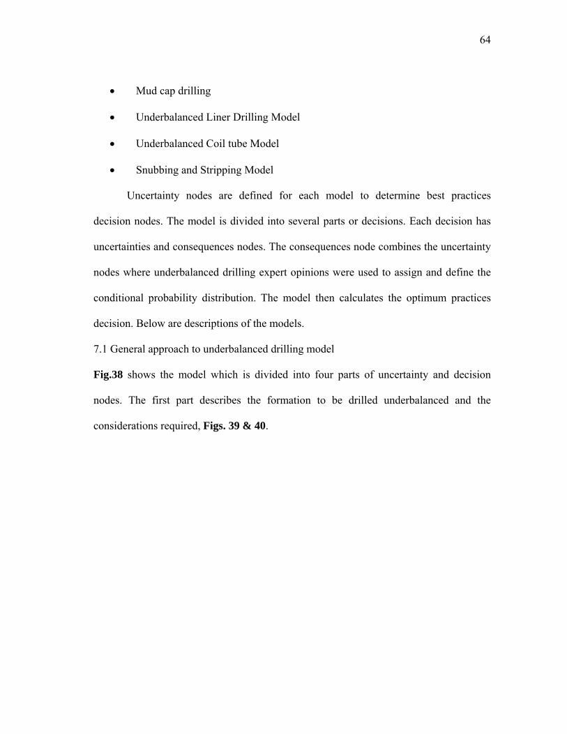
64

• Mud cap drilling

• Underbalanced Liner Drilling Model

• Underbalanced Coil tube Model

• Snubbing and Stripping Model

Uncertainty nodes are defined for each model to determine best practices

decision nodes. The model is divided into several parts or decisions. Each decision has

uncertainties and consequences nodes. The consequences node combines the uncertainty

nodes where underbalanced drilling expert opinions were used to assign and define the

conditional probability distribution. The model then calculates the optimum practices

decision. Below are descriptions of the models.

7.1 General approach to underbalanced drilling model

Fig.38 shows the model which is divided into four parts of uncertainty and decision

nodes. The first part describes the formation to be drilled underbalanced and the

considerations required, Figs. 39 & 40.

65

Fig.38: General approach to underbalanced drilling

Fig.39: Formations indicators list that need to be considered

66

Fig.40: A list of considerations for the different formations indicators available

The second part shows the planning phases’ uncertainty (Fig.41) and its

corresponding recommendations, Fig.42.

67

Fig.41: Planning phases

Fig.42: Planning phases recommendations

68

The third part shows the equipments requirement uncertainty node or options

(Fig.43) and its corresponding decision (equipment recommendations).

Fig.43: A list of equipments required

69

The fourth part shows the operations planning probability and its corresponding

decisions, Fig.44.

Fig.44: A list of operating planning

7.2 Flow underbalanced drilling model

Fig.45 shows the overall model of flow UBD. The model is divided into three parts

(tripping, connection and flow drilling uncertainty and decision nodes).

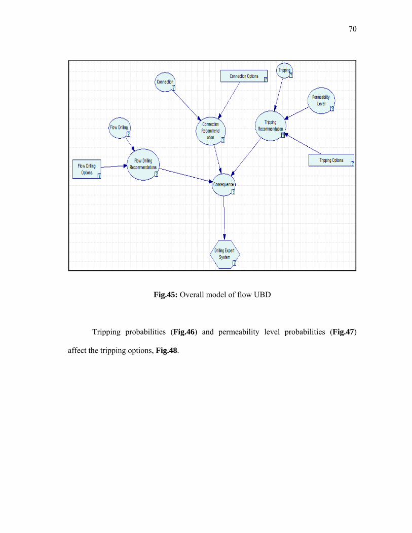
70

Fig.45: Overall model of flow UBD

Tripping probabilities (Fig.46) and permeability level probabilities (Fig.47)

affect the tripping options, Fig.48.

71

Fig.46: Tripping options in flow UBD

Fig.47: Permeability level options in flow UBD

72

Fig.48: A list of tripping recommendations

The second part is the connection probabilities (Fig. 49) and connection options,

Fig. 50. The third part is related to flow drilling operations, Fig. 51.

73

Fig.49: Connection options

Fig.50: Connection recommendations

74

Fig.51: Flow drilling options

If the tripping probability is selected as RIH (Fig.52) and high permeability level

(Fig.53) then the optimum tripping operation is to use mud cap, Fig. 54.

Fig.52: The user selects RIH option

75

Fig.53: The user selects high permeability option

Fig.54: Tripping recommendation for low permeability formation during RIH operation

76

Selection of on connection probability (Fig.55) leads to optimum connection

option shown in Fig.56.

Fig.55: The user selects on connection option

Fig.56: Connection recommendation

77

Selection of flow drilling with formation gas or fluid returns (Fig. 57) leads to

the optimum practice shown in Fig.58.

Fig.57: The user selects flow drilling takes place in formation with gas or fluid returns

Fig.58: The recommended flow drilling with formation gas or fluid returns

78

7.3 Gaseated underbalanced drilling model

Fig.59 shows the overall model of gaseated UBD. The model is divided into four parts

(selection method benefits and challenges, requirements for general limits of gas and

fluid volume, operational concerns and challenges recommendations, and well kicks

recommendations.

Fig.59: Overall model for gaseated UBD

Selection method probabilities are shown in Fig.60 and general limits of gas and

fluid volume probabilities are shown in Fig.61.

79

Fig.60: A list of gaseated methods

Fig.61: Possible general limits of gas and fluid volume

80

Operational concerns and challenges are shown in Fig. 62 and kick types

probabilities are shown in Fig. 63.

Fig.62: Possible operational concerns and challenges

Fig.63: Possible kick types

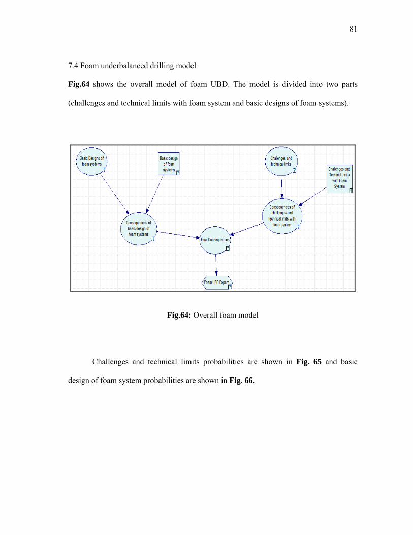
81

7.4 Foam underbalanced drilling model

Fig.64 shows the overall model of foam UBD. The model is divided into two parts

(challenges and technical limits with foam system and basic designs of foam systems).

Fig.64: Overall foam model

Challenges and technical limits probabilities are shown in Fig. 65 and basic

design of foam system probabilities are shown in Fig. 66.

82

Fig.65: Possible challenges and technical limits of foam UBD

Fig.66: A list of basic designing steps in foam UBD

83

7.5 Air and gas underbalanced drilling model

Fig.67 shows the overall model of air and gas UBD. The model is divided into four

parts. The first part is rotary and hammers drilling probabilities and recommendations.

The second part is limits and challenges to gas drilling probabilities and

recommendations. The third part is rig requirements and recommendations. The fourth

part is gas drilling operations probabilities and recommendations.

Fig.67: Overall air and gas UBD

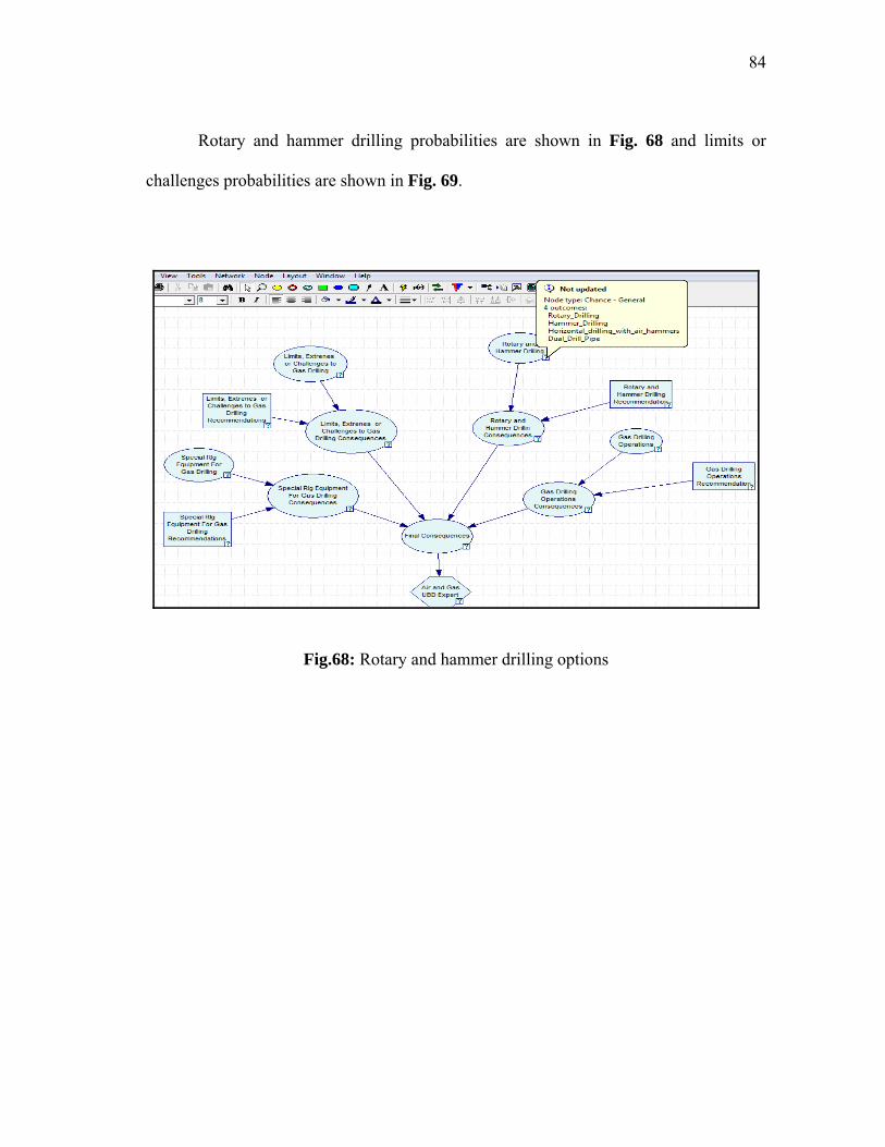
84

Rotary and hammer drilling probabilities are shown in Fig. 68 and limits or

challenges probabilities are shown in Fig. 69.

Fig.68: Rotary and hammer drilling options

85

Fig.69: A list of limits and challenges for air and gas UBD

Gas drilling operation probabilities are shown in Fig. 70 and special rig

equipment for gas drilling probabilities are shown in Fig. 71.

86

Fig.70: A list of possible gas drilling operations

87

Fig.71: A list of possible rig equipment for gas drilling

7.6 Mud cap model

Fig.72 shows the overall model of mud cap model. The model is divided into three parts.

The first part is background to mud cap drilling probabilities and recommendations. The

second part is drilling problems probabilities and recommendations. The third part is

floating mud cap drilling in depleted formation probabilities and recommendations.

88

Fig.72: Mud cap overall model

Background mud cap drilling probabilities are shown in Fig. 73 and drilling

problems probabilities are shown in Fig. 74.

Fig.73: A list of background mud cap drilling

89

Fig.74: A list of mud cap drilling problems

Floating mud cap drilling in depleted formation probabilities are shown in Fig.

75.

Fig.75: Floating mud cap drilling options

90

7.7 Underbalanced liner drilling model

Fig.76 shows the overall model of UBLD model. The model is divided into three parts.

The first part is basic planning probabilities and recommendations. The second part is

drilling problems that can be solved and recommendations. The third part is limits and

challenges probabilities and recommendations.

Fig.76: Overall model for UBLD

Problems that can be solved by UBLD (Fig. 77) and limits and challenges

probabilities are shown in Fig. 78. Basic planning probabilities are shown in Fig. 79

91

Fig.77: A list of problems that can be solved by UBLD

Fig.78: Limits and challenges with UBLD

92

Fig.79: Basic planning for UBLD options

7.8 Underbalanced coil tube model

Fig.80 shows the overall model of UBCT model. The model is divided into two parts.

The first part is pre-planning probabilities and requirements. The second part is drilling

challenges probabilities and solutions.

Fig.80: Overall model for UBCT

93

Pre-planning probabilities are shown in Fig. 81 and drilling challenges

probabilities are shown in Fig. 82.

Fig.81: A list of pre-planning possibilities

94

Fig.82: A list drilling challenges with UBCTD 7.9 Snubbing and stripping model

Fig.83 shows the overall model of snubbing and stripping model. The model is divided

into four parts. The first part is basic snubbing probabilities and recommendations. The

second part is snubbing units’ probabilities and recommendations. The third part is

general stripping procedure and recommendations. The fourth part is snubbing

operations probabilities and its recommendations.

95

Fig.83: Overall model for snubbing and stripping

Basic snubbing probabilities (Fig. 84) and snubbing units’ probabilities are

shown in Fig. 85.

96

Fig.84: A list of basic snubbing options

Fig.85: A list of snubbing unit

97

General stripping procedure (Fig. 86) and snubbing operations probabilities are

shown in Fig. 87.

Fig.86: A list of possible stripping procedure

Fig.87: A list of possible snubbing operations

98

CHAPTER VIII

RESULTS AND DISCUSSION*

In this chapter, examples for different scenarios are shown and explained from the

models developed here. This chapter is divided into five sections (completion, drilling

fluids, well control, cementing, and underbalanced drilling).

____________

*Reprinted with permission from “Expert System for the Optimal Design and Execution of Successful Completion Practices Using Artificial Bayesian Intelligence,” by Al-Yami, A.S., Schubert, J., and Beck, G., 2011, SPE 143826, Copyright © 2012, Society of Petroleum Engineers.

*Reprinted with permission from “Drilling Fluids Consultation System: Development and Field Applications,” by Al-Yami, A.S. and Schubert, J., 2012a, SPE 152098, Copyright © 2012, Society of Petroleum Engineers.

*Reprinted with permission from “Development of Optimum Well Control Practices Using Artificial Bayesian Intelligence,” by Al-Yami, A.S. and Schubert, J., 2012c, OTC 22882, Copyright © 2012, Society of Petroleum Engineers. *Reprinted with permission from “Drilling Expert System for the Optimal Design and Execution of Successful Cementing Practices,” by Al-Yami, A.S., Schubert, J., Medina, C., and Ok-Youn, Y., 2010b, IADC/SPE 135183, Copyright © 2010, Society of Petroleum Engineers

*Reprinted with permission from “Guidelines for Optimum Underbalanced Drilling Practices Using Artificial Bayesian Intelligence,” by Al-Yami, A.S. and Schubert, J., 2012d, OTC 22883, Copyright © 2012, Society of Petroleum Engineers.

99

8.1 Well Completion model

This section shows the use of this model in one scenario where the user selects his

conditions, Figs. 88-93. To view the results once the model is executed can be done by

obtaining the optimum results from each section separately, Figs. 94-100. Figs. 98 and

99 shows that no need to do perforation or openhole gravel packing since our optimum

lateral completion is openhole expandable screens. If we change the four uncertainties

(cost, zonal isolation, reliability and productivity) to (moderate, poor, moderate, and

good) then our optimum lateral completion will be openhole gravel packing, Fig.101.

Since the lateral completion is openhole gravel packing, the user can get more details by

selecting his desired conditions, Fig.102-103. The optimum slurry density for openhole

gravel packs is shown in Fig. 104.

100

Fig.88: Selection of considerations of designing a multilateral junction

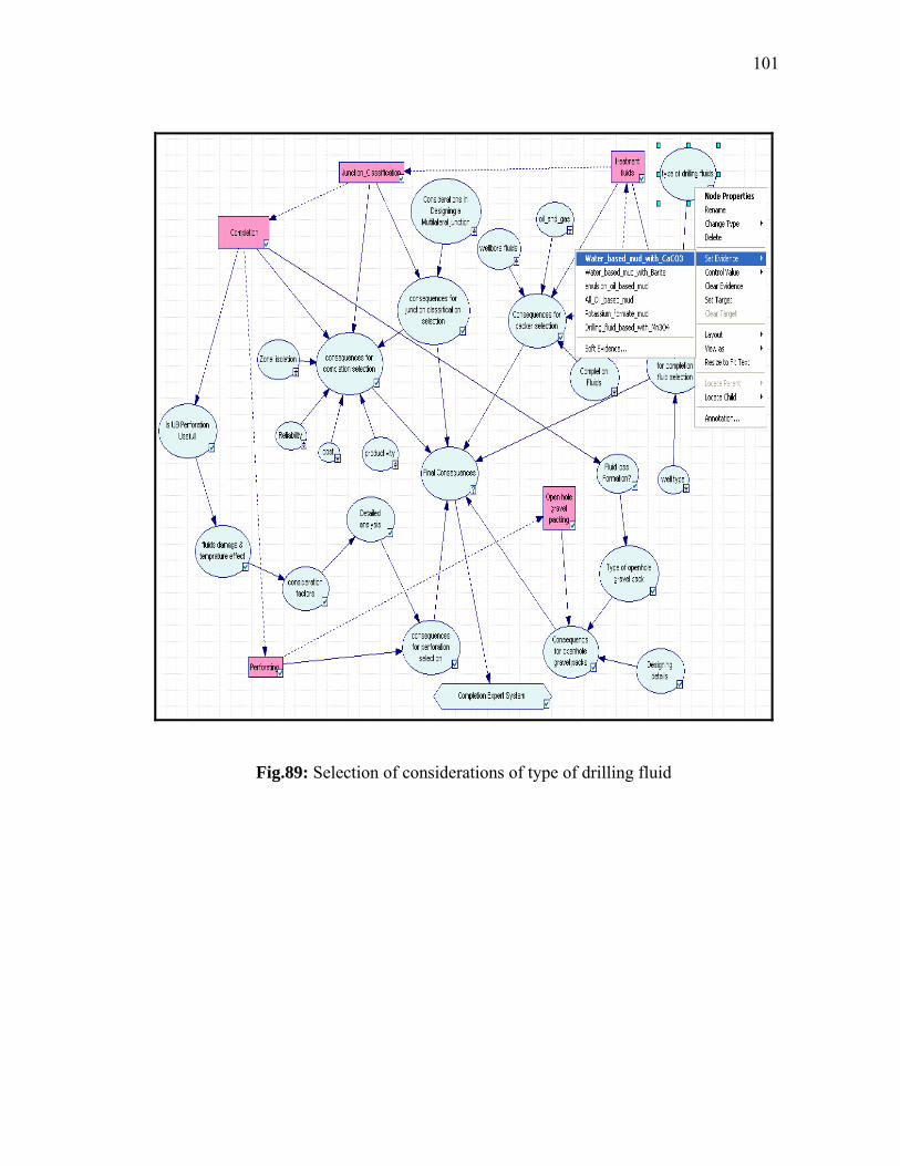
101

Fig.89: Selection of considerations of type of drilling fluid

102

Fig.90: Selection of well type

103

Fig.91: Selection of completion fluids

104

Fig.92: Selection of oil and gas characteristics

105

Fig.93: Selection of wellbore fluids

Fig.94: Optimum selection of junction classification

106

Fig.95: Optimum selection of completion (treatment) fluid

Fig.96: Optimum selection of completion selection

Fig.97: Optimum selection of perforation selection

107

Fig.98: Optimum selection of openhole gravel packs details

Fig.99: Optimum selection of packers

Fig.100: Optimum selection of completion (openhole gravel pack) selection for different conditions

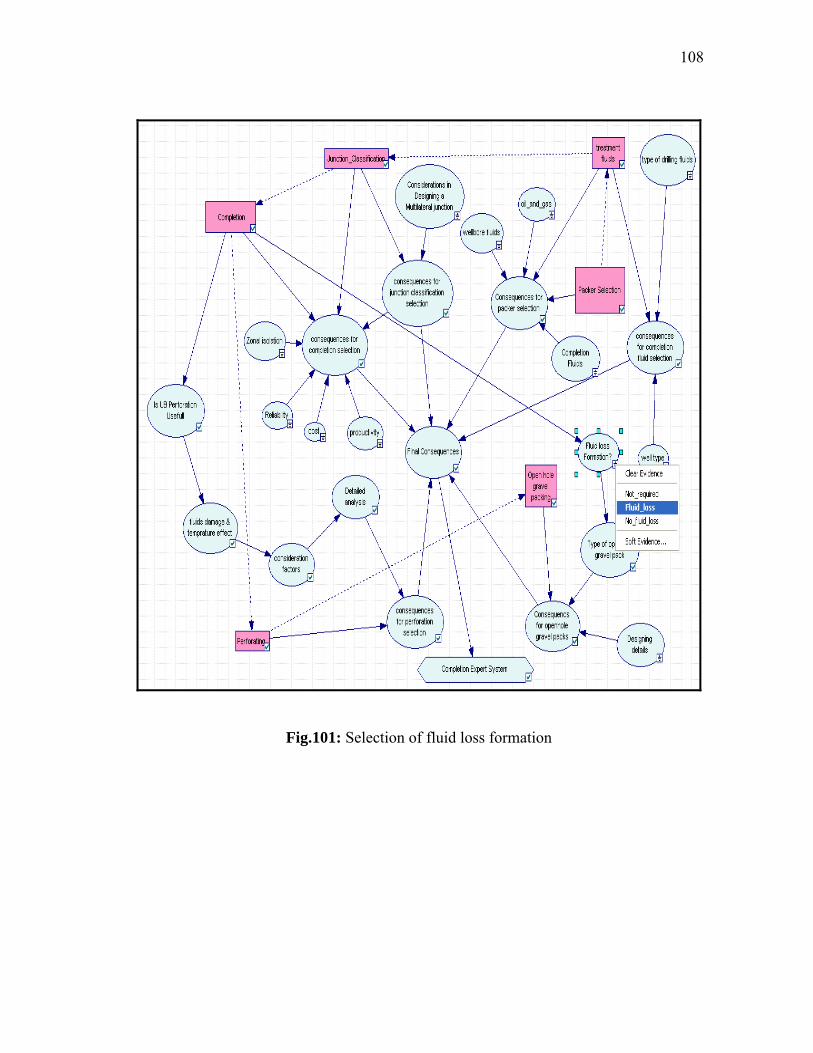
108

Fig.101: Selection of fluid loss formation

109

Fig.102: Selection of required slurry density from designing details

Fig.103: part of consequences of openhole gravel packs showing optimum slurry density

The above example showed how using the model in selecting the optimum

practices for junction classification, treatment fluid, lateral completion, perforation,

110

openhole gravel packing, and packer selection. The states of probabilities in the above

tables were obtained by literature review and experts opinions. In case new practices or

different experts’ opinions are presented then all we need to do is simply change the

states of probabilities. In case that the above model is missing other factors then we can

also update the model and its corresponding states of probabilities. The flexibility of

Bayesian Network in terms of updating the structure model and its beliefs makes this

method the first systematic approach to build experts systems.

The main borehole and the lateral are cased and cemented in level 4 completion.

In level 3, the mechanical integrity by casing is only observed at the junction. Level 4

requires cementing at the junction resulting in enhanced mechanical integrity and

hydraulic isolation, Hill et al. (2008).

Acidic completion brines utilizing HCl are not effective in removing filter cake

in long contact horizontal reservoirs. Lactic, acetic esters showed promising results in

removal filter cake from water based drilling fluids, Al-Yami et al. (2009).

Openhole expandable screen lateral completion is selected because the user

wants good productivity, cost and zonal isolation. Skin factors close to zero have been

observed in the field when using expandable screens. The cost is higher than standalone

screen but cheaper than openhole gravel packs, cased hole gravel packs and frac packs.

Good zonal isolation has been observed in the field, Jonathan (2009).

Once we change the four uncertainties (cost, zonal isolation, reliability and

productivity) to (moderate, poor, moderate, and good) the optimum lateral completion

will be openhole gravel packing.

111

Basically there are two ways to perform openhole gravel packs. The first one is

alternate path which is suitable when we have lost circulation formation. The other way

is circulating pack which requires full returns. The user selected lost circulation

formation and wants to know the required slurry density. Higher concentration around 8

ppa (pound of proppant added per gallon of clean fluid) is required for alternate path

open hole gravel packs, Jonathan (2009).

One of the packers selected was oil swelling packers. Studies done by Al-Yami

et al. (2008) showed that they are resistant against different salinity fluids and acids.

Water swelling packers are not selected because they can be damaged by CaCl2 fluids

and strong acids, Al-Yami et al. (2010a)

8.2 Drilling fluids model

The user can select the potential hole problem that might be faced by assigning a

probability of one to any of the available probabilities. For example the user selects

potential formation damage, Fig.104. A temperature range of 220 to 330 °F was

selected, Fig. 105. The utility node named drilling fluid expert system shows examples

of recommended drilling fluids, Figs.106&107.

112

Fig.104: Selecting formation damage as a potential hole problem (example 1)

Fig.105: Selecting temperature range (example 1)

113

Fig.106: Some possible drilling fluids recommendation for the conditions user selected (example 1)

Fig.107: More possible drilling fluids recommendation for the conditions user selected (example 1)

Selection of 120 to 220 °F range (Fig.108) and loss of circulation and water

flows (Fig.109) can lead to another example of drilling fluid recommendation, Fig.110.

114

Fig.108: Selecting temperature range (example 2)

Fig.109: Selecting loss of circulation and water flows as a potential hole problem (example 2)

115

Fig.110: Formulation 7 is an example of a drilling fluid that will work in the selected conditions (example 2)

Selection of 220 to 330 °F range (Fig.111) and tight hole and flow with abnormal

pressure (Fig.112) can lead to another example of drilling fluid recommendation,

Figs.113 & 114.

Fig.111: Selecting temperature range (example 3)

116

Fig.112: Selecting loss of circulation and water flows as a potential hole problem (example 3)

Fig.113: Formulation 24 is an example of a drilling fluid that will work in the selected

conditions (example 3)

Fig.114: Formulation 47 is another example of a drilling fluid that will work in the selected conditions (example 3)

117

If the user only knows the temperature range (Fig.115) and formation name

(Fig.116) he can still use the model since the potential hole problems is affected by the

formation name. Selecting Arab-D formation leads to five potential hole problems

probabilities shown in Fig.117. Different drilling fluids formation can be used in this

case, Fig.118.

Fig.115: Selecting temperature range (example 4)

Fig.116: Selecting Saudi Arabia formation (example 4)

118

Fig.117: Showing resultant potential hole problems in Arab D formation as selected

before (example 4)

Fig.118: Drilling fluid 23 is the optimum fluid in this case (example 4)

A temperature probability of 120 to 220 °F (Fig.119) and Wasia and Shuaiba

formation (Fig.120) are selected. Wasia and Shuaiba formation is considered to be a

119

tight hole and a lost circulation zone, Fig.121. Different drilling fluids formulations are

recommended by the drilling fluid model, Figs. 122 & 123.

Fig.119: Selecting temperature range (example 5)

Fig.120: Selecting Saudi Arabia formation (example 5)

120

Fig.121: Showing resultant potential hole problems in Wasia and Shuaiba formations as selected before (example 5)

Fig.122: Showing some recommended drilling fluids for the above conditions (example 5)

121

Fig.123: Showing more recommended drilling fluids for the above conditions (example 5)

Selection of a higher temperature range probability of 330 to 400 °F (Fig.124)

and potential formation damage problem, Fig.125 leads to different drilling fluids

formulations recommended by the drilling fluid model, Fig.126.

Fig.124: Selecting temperature range (example 6)

122

Fig.125: Selecting potential hole problem (example 6)

Fig.126: Showing the recommended drilling fluids for the above conditions (example 6)

The above example showed how using the model in selecting the optimum

practices for drilling fluids selection. The states of probabilities in the above tables were

obtained by experts’ opinions. In case new practices or different experts’ opinions are

presented then all we need to do is simply change the states of probabilities. In case that

the above model is missing other factors then we can also update the model and its

corresponding states of probabilities. The flexibility of Bayesian Network in terms of

123

updating the structure model and its beliefs makes this method the first systematic

approach to build experts systems.

Selecting the acid soluble clay free NaCl brine drill-in fluid is an optimum

selection to minimize formation damage problems. The polymers included in the design

are suitable for the temperature range selected.

Using Barite or CaCO3 fine can be used to increase the mud density as hole

conditions dictate to control water flow potential problem mentioned in example 2. For

the lost circulation problem, treatment with lost circulation material should help to cure

the lost circulation zone.

Inhibitive KCl drilling fluid looks like a good choice since tight hole is a

potential problem. Using Barite or CaCO3 can be used to increase the mud density to

minimize the flow and abnormal pressure problem.

Wasia and Shuaiba formations are considered to be a tight hole and a lost

circulation zone. Spud mud made up of pre-hydrated bentonite in freshwater and

flocculated with lime should be sufficient to drill this interval. Curing lost circulation

should be considered but in case it does not work. Drilling with water should not be

practiced here which is in agreement with the model recommendation.

For temperature higher than 330°F and in a zone with high potential for

formation damage, potassium formate can be considered as a good drilling fluid.

Downs (1992) listed some advantages of having the formate brines that make it

ideal drill-in fluid. Some of these advantages are:

• Maintenance of rheological properties at high temperatures

124

• Minimal circulating pressure losses

• Elimination of solids sag at high temperatures

• Low potential for differential sticking

• Very thin filter cake

• Low ECD ( equivalent circulating density) in long and narrow hole sections

Brinkhorst (1994) mentioned that the potassium formate was used successfully to

drill Norwegian field and no damaging effects were observed.

8.3 Well control model

The user can select the kick indication observed by assigning a probability of one to any

of the available probabilities. For example the user selects increase in flow and pit gain,

Fig.127. Once the kick has been verified (Fig.128) the user needs to select his kick

details. The kick is from a horizontal or deviated well, Fig.129. Then the optimum

circulation method is the driller method as shown in Fig. 130.

125

Fig.127: Kick indicator example

Fig.128: Verification of the kick

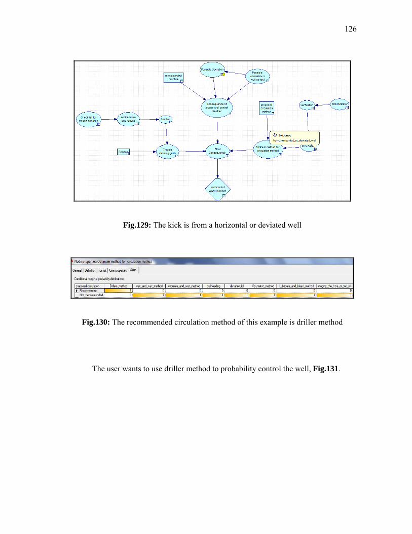
126

Fig.129: The kick is from a horizontal or deviated well

Fig.130: The recommended circulation method of this example is driller method

The user wants to use driller method to probability control the well, Fig.131.

127

Fig.131: The user is controlling the well using driller method

The user enters his probability conditions from the possible operation node

(Fig.132) and the recommended practice of increasing pump rate is calculated by the

model, Fig. 133.

128

Fig.132: The user is entering his pipe, casing and pump operational conditions

Fig.133: The optimum practice of proper well control is shown

129

The user selects that drill pipe pressure is up and casing pressure is up about the

same amount as the drill pipe pressure, Fig.134. Possible probabilities due to the

selection from the check list for trouble shooting node are shown in Fig.135.

Fig.134: The user shows his problem by selecting drill pipe and casing pressure

response

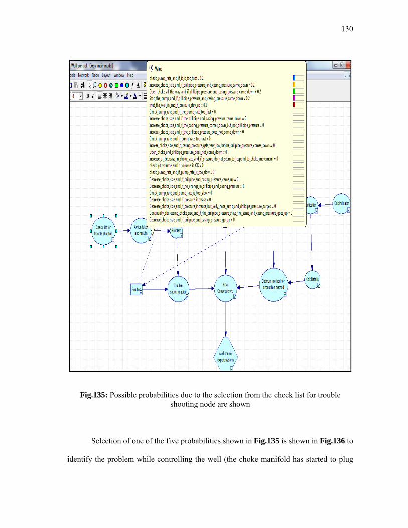
130

Fig.135: Possible probabilities due to the selection from the check list for trouble shooting node are shown

Selection of one of the five probabilities shown in Fig.135 is shown in Fig.136 to

identify the problem while controlling the well (the choke manifold has started to plug

131

up), Fig.137. The optimum solution is calculated by the model to switch to alternate

choke line and clear the manifold, Fig.138. Again, expert opinions are used here in the

trouble shooting guide consequence which can be updated easily in case of different

opinions or field cases.

Fig.136: The user then selects an action and its corresponding result in an attempt to identify the problem

132

Fig.137: The problem is identified

Fig.138: A recommendation is given to solve this problem

133

If no pre-recorded data is available probability is selected (Fig.139) and a

possible operation is selected (Fig.140) then the optimum well control practice is

calculated as shown in Fig. 141.

Fig.139: The user is controlling the well without any prerecorded data

Fig.140: The user is entering his observations

134

Fig.141: The recommended proper well control practice is shown

Additional examples of proper well control part are shown below. Figs 142-144

is related to pumps troubles during a kick. Figs. 145-147 are related to having a kick in

deep water.

Fig.142: The user is controlling the well and he has pump troubles during a kick

135

Fig.143: The user is entering his observations during the pump trouble

Fig.144: The recommended proper well control practice is shown for the selected conditions for the pump trouble during a kick

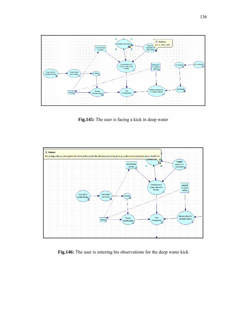
136

Fig.145: The user is facing a kick in deep water

Fig.146: The user is entering his observations for the deep water kick

137

Fig.147: The recommendation for the kick in deep water

The above example showed how using the model in selecting the optimum

practices for well control. The states of probabilities in the above tables were obtained

by experts’ opinions. In case new practices or different experts’ opinions are presented

then all we need to do is simply change the states of probabilities. In case that the above

model is missing other factors then we can also update the model and its corresponding

states of probabilities. The flexibility of Bayesian Network in terms of updating the

structure model and its beliefs makes this method the first systematic approach to build

experts systems.

In Figs.129 and 130 the Driller’s method is well suited for horizontal well

control, as immediate circulation is important. Using the Driller’s method can help in

avoiding complicated pressure schedule calculations associated with the Wait and

Weight method. Driller’s method is simple and is considered to be a good circulation

method in horizontal well control situations, GRØTTHEIM (2005).

In Figs. 132 and 133, increasing pump rate is recommended to avoid another

bubble from entering the bore hole on bottom. In Figs.143 and 144, stopping the pump

and closing in the well is the recommended practice because the well cannot be killed if

138

the pump rate is not constant. The increase in pump rate and decrease in pipe pressure

might indicate a hole in the drill pipe or a bad pump. The instability movement of the

Kelly hose might indicate that the problem is at the pump.

The third part in the above model is designed to assist the user to find the

optimum solution for a list of potential problems that can be faced during well control

operations. In general there are rules that can serve as good guides, Rehm et al. (1975):

• Unstable movement of Kelly hose or surging pump pressure gauge is a sign of

pump problems.

• If the pipe pressure only goes up then the bit or nozzle is plugged.

• If the drill pipe and casing pressure increase suddenly then the choke or manifold

is plugged.

• If the drill pipe pressure is decreased then there might be a hole in the pipe.

• If the drill pipe pressure and casing pressure does not respond to the choke, you

might have a lost circulation problem.

8.4 Cementing model

This section shows the use of this model in one scenario where the user select his

conditions, Figs.148-151. The conditions are:

• Well Type: Oil well

• Bottom Hole Static Temperature: 300-400°F

• Objective: Production Liner

• Drilling Fluid Type: Water based mud

139

Fig.148: Selection of well type

Fig.149: Selection of bottom hole static temperature

140

Fig.150: Selection of well objective

141

Fig.151: Selection of drilling fluid

The consequences node combines the four uncertainty nodes (well type, required

pumping time, objective and drilling fluid) and the three decision nodes (recommended

cement formulations, recommended spacers and recommended operational practices).

Cementing expert opinion was used to assign and define the node conditional probability

distribution. The model then calculate based on the given above conditions that the

optimum practice to cement the liner, Figs.152-153.

142

Fig.152: The cementing expert system recommends formulation 13, operational note 5

and spacer 2 to be used in this application

143

Fig.153: The model showing more details for this application (Example 1)

144

Another example is shown below:

• Well Type: Gas well

• Bottom Hole Static Temperature: 300-400°F

• Objective: Long Liner

• Drilling Fluid Type: Oil based mud

The model then calculates and shows in Fig.154 the optimum practice to cement the

long liner.

145

Fig.154: The model showing more details for this application (Example 2)

146

The drilling expert system for cement was based on field and lab experience. It is

not possible to outline this in this manuscript. For the first example, selection of the

following cement slurry design: Cement +35%BWOC silica flour+Expansion

additive+Dispersant+ Fluid loss additive+ Retarder+ 0.01 gps Antifoaming agent is

suitable. The temperature is high (300-400 °F) which requires the use of retarder to delay

setting of cement. Lignosulfonate and some carbohydrate derivatives such as xanthan

gum, cellulose and polyanionic cellulose are common retarders. Viscosity of cement

slurry also affect pumping properties, at high temperature the viscosity will be reduced

which might lead to solids settling. To solve this problem, additives for viscosity control

are used. Dispersants are used with cement slurry to improve the rheological

performance especially at higher densities without the use of additional water.

Expansion additives (for example CaO or MgO) are used to minimize shrinkage during

cement slurry setting. The expansion additives are effective when bottom hole

temperature is greater than approximately 300 °F. Fluid loss additives are used to

minimize hydration of water sensitive shale, to maintain the cement slurry water for the

hydration process, and to minimize bridging in wellbore. Also the use of silica source is

required to prevent strength regression.

Water based spacer can be used since we are using water based drilling fluid. The

operational note indicates best field cementing practice for this case as the following:

1. Liner hanger representative should be on the rig floor at all times while the

liner is being RIH especially when being rotated (via rotary table with DP in the slips),

147

and should ensure that the rotation torque at 15 RPM or lower does not exceed the

maximum allowed rotating torque.

2. Pump enough spacer and cement

3. Pay attention to difference in temperature in case of long liners. Compressive

strength of 500 psi is required at the top of the liner

4. After starting to pump cement downhole, begin to rotate the liner at 3 to 7

RPM. If observed surface torque is below maximum allowed surface torque, increase

RPM to 15, otherwise attempt to rotate at any lower RPM if the observed surface torque

is less than maximum allowable surface torque, up until plug bumps.

5. Actual volumes will be based on openhole caliper log.

6. Cement additives maybe revised after final confirmation testing

7. Cement will be batch mixed

8. Pump fresh water behind wiper plug and cement in lines ahead of water (1-2

bbl).

9. Slow displacement to 2-3 bpm before sharing the liner wiper plug. Do not

over displace.

10. Record the maximum surface rotating torque observed during the cement job

on the drilling report.

11. Pull four stands above the liner top and reverse circulation 1.5 DP volumes.

Pull additional 5 stands and reverse out 1.5 DP volumes. Shut in well and apply 300-400

psi. WOC for 7 hours. Flow check then POH laying-down excess DP and liner setting

tool.

148

12. When RIH with bit to drill top of liner cement, if no solid cement can be

observed within 15-20 feet on TOL then wait for longer time for cement to develop the

required compressive strength. It should be noted that having soft cement at the top of

the liner can be due to contaminants which may not indicate cement failure.

For the second example (cementing Gas Long Production Liner), the same

operational field note above can be applied. The spacer will be a water based spacer that

has mutual solvent to water wet the formation for improved formation cement bonding,

Since we have a long gas production liner the cement slurries should meet the

following requirements, Al-Yami et al. (2007):

1. The thickening time must be sufficient to allow proper slurry placement.

2. Rapid compressive strength development at the top of the liner and the

bottom.

3. The slurry must be easily mixable and must not exhibit free water or settling

tendencies.

4. A fluid-loss of ≤ 100 ml/30 min.

In addition to conventional additives such as fluid loss, dispersants, silica source

latex must be used:

For wells that show high gas migration potential we can use latex additive. Latex

is a copolymer of AMPS, N-Vinylacylamide and acrylamide, Fink (2003). The

following retarders’ combinations are recommended Al-Yami et al. (2007):

• Blend of salt and organic acid.

• Aromatic polymer derivative and blend of salt and organic acid.

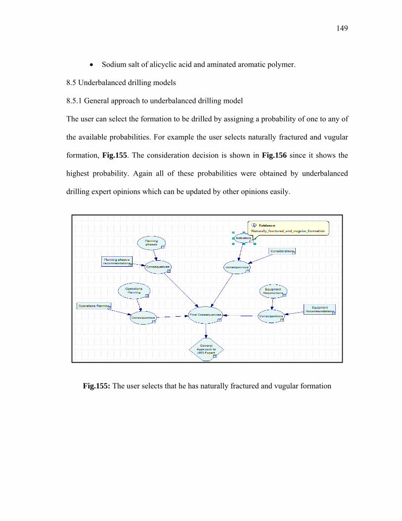
149

• Sodium salt of alicyclic acid and aminated aromatic polymer.

8.5 Underbalanced drilling models

8.5.1 General approach to underbalanced drilling model

The user can select the formation to be drilled by assigning a probability of one to any of

the available probabilities. For example the user selects naturally fractured and vugular

formation, Fig.155. The consideration decision is shown in Fig.156 since it shows the

highest probability. Again all of these probabilities were obtained by underbalanced

drilling expert opinions which can be updated by other opinions easily.

Fig.155: The user selects that he has naturally fractured and vugular formation

150

Fig.156: The consideration decision 8.5.2 Flow underbalanced drilling model

If the tripping probability is selected as RIH (Fig.157) and high permeability level

(Fig.158) then the optimum tripping operation is to use mud cap, Fig. 159.

Fig.157: The user selects RIH option

151

Fig.158: The user selects high permeability option

152

Fig.159: Tripping recommendation for low permeability formation during RIH operation

Selection of on connection probability (Fig.160) leads to optimum connection

option shown in Fig.161.

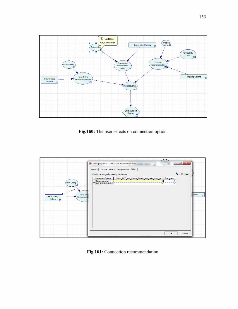
153

Fig.160: The user selects on connection option

Fig.161: Connection recommendation

154

Selection of flow drilling with formation gas or fluid returns (Fig. 162) leads to

the optimum practice shown in Fig.163.

Fig.162: The user selects flow drilling takes place in formation with gas or fluid returns

Fig.163: The recommended flow drilling with formation gas or fluid returns

155

8.5.3 Gaseated underbalanced drilling model

Selection of concentric casing string injection method (Fig. 164) leads to benefits and

challenges shown in Fig.165.

Fig.164: The user selects gaseated UBD method (dual casing string)

156

Fig.165: The recommendation for dual casing string is shown

Selection of back pressure gas and fluid limitation probability (Fig. 166) leads to

the optimum recommendation shown in Fig.167.

157

Fig.166: The user selects general limit of gas and fluid volume (back pressure)

Fig.167: Back pressure recommendation

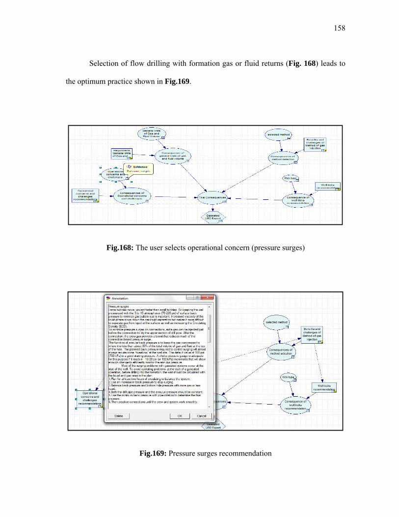
158

Selection of flow drilling with formation gas or fluid returns (Fig. 168) leads to

the optimum practice shown in Fig.169.

Fig.168: The user selects operational concern (pressure surges)

Fig.169: Pressure surges recommendation

159

Selection of gas flow kick type (Fig. 170) leads to the optimum well kick

recommendation shown in Fig.171.

Fig.170: Selecting kick type (gas flow)

160

Fig.171: Recommendation for kick type (gas flow)

8.5.4 Foam underbalanced drilling model

Selection of hot holes as a challenge (Fig. 172) leads to the optimum recommendation

shown in Fig.173.

161

Fig.172: The user selects hot holes as a challenge

Fig.173: Hot holes recommendation

Selection of making a connection in foam underbalanced drilling (Fig. 174) leads

to the optimum connection procedure detailed in Fig.175.

162

Fig.174: Selecting basic designing in making a connection in foam UBD

Fig.175: Recommendation for making a connection in foam UBD

8.5.5 Air and gas underbalanced drilling model

Selection of horizontal drilling with air hammers (Fig. 176) leads to the optimum

recommendation detailed in Fig.177.

163

Fig.176: Selecting horizontal drilling with air hammers

164

Fig.177: Recommendation for horizontal drilling with air hammers

Selection of water or wet holes probability as a challenge to gas drilling (Fig.

178) leads to the optimum recommendation detailed in Fig.179.

Fig.178: Selection of water or wet holes as a challenge

165

Fig.179: Water or wet holes recommendation

Selection of mist pump rig equipment probability (Fig. 180) leads to the

optimum recommendation detailed in Fig.181.

166

Fig.180: Selection of mist pumps

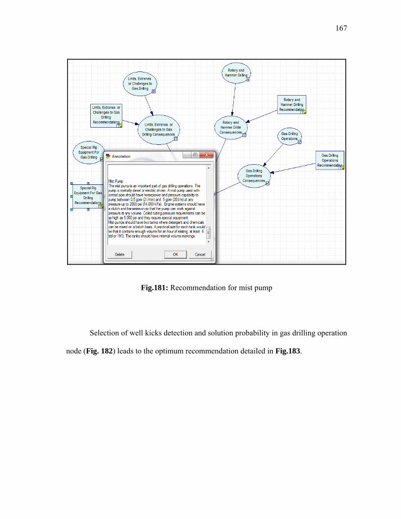
167

Fig.181: Recommendation for mist pump

Selection of well kicks detection and solution probability in gas drilling operation

node (Fig. 182) leads to the optimum recommendation detailed in Fig.183.

168

Fig.182: Selection of gas drilling operations (well kicks detection and solution)

Fig.183: Well kicks detection and solution recommendation

169

8.5.6 Mud cap model Selection of trips with pressurized mud caps probability (Fig. 184) leads to the optimum

recommendation detailed in Fig.185.

Fig.184: Selecting trips with pressurized mud caps

Fig.185: Recommendation for trips with pressurized mud caps

170

Selection of drilling ahead with mud losses probability in drilling problem node

(Fig. 186) leads to the optimum recommendation detailed in Fig.187.

Fig.186: Selection of drilling ahead with mud losses

171

Fig.187: Recommendation for drilling ahead with mud losses

Selection of water sensitive formation exposed probability (Fig. 188) leads to the

optimum recommendation detailed in Fig.189.

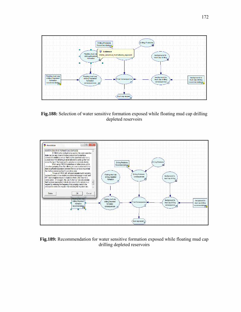
172

Fig.188: Selection of water sensitive formation exposed while floating mud cap drilling depleted reservoirs

Fig.189: Recommendation for water sensitive formation exposed while floating mud cap drilling depleted reservoirs

173

8.5.7 Underbalanced liner drilling model

Selection of the bit probability in basic planning node (Fig. 190) leads to the optimum

recommendation detailed in Fig.191.

Fig.190: Selection of basic planning of the bit

174

Fig.191: Recommendation for the bit used in UBLD

Selection of wellbore ballooning probability (Fig. 192) leads to the optimum

recommendation detailed in Fig.193.

Fig.192: Selection of the potential problem (hole ballooning)

175

Fig.193: Showing how UBLD can solve the potential problem (hole ballooning)

Selection of liner hanger challenge probability (Fig. 194) leads to the optimum

recommendation detailed in Fig.195.

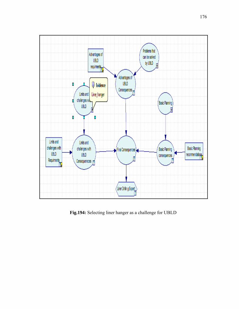
176

Fig.194: Selecting liner hanger as a challenge for UBLD

177

Fig.195: Recommendation for the liner hanger in UBLD

Selection of drilling fluid considerations probability (Fig. 196) leads to the

optimum recommendation detailed in Fig.197.

178

Fig.196: Selecting drilling fluids as a challenge for UBLD

Fig.197: Recommendation for drilling fluids in UBLD

179

8.5.8 Underbalanced coil tube model Selection of pressure categories and BOP stack requirement probability (Fig. 198) leads

to the optimum requirement detailed in Fig.199.

Fig.198: Selecting pre-planning option of BOP stack requirement

180

Fig.199: Recommendation of pre-planning option of BOP stack requirement

Selection of ROP reduction challenge probability (Fig. 200) leads to the

optimum recommendation detailed in Fig.201.

Fig.200: Selection of ROP reduction challenge in UBCTD

181

Fig.201: Recommendation for ROP reduction challenge in UBCTD

8.5.9 Snubbing and stripping model

Selection of stripping with annular preventer probability (Fig. 202) leads to the optimum

recommendation detailed in Fig.203.

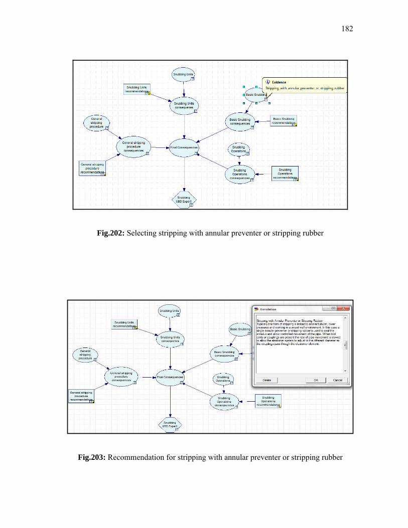
182

Fig.202: Selecting stripping with annular preventer or stripping rubber

Fig.203: Recommendation for stripping with annular preventer or stripping rubber

183

Selection of auxiliary equipment probability (Fig. 204) leads to the optimum

recommendation detailed in Fig.205.

Fig.204: Selection of auxiliary equipment from snubbing unit options

184

Fig.205: Recommendation for auxiliary equipment from snubbing unit options

Selection of ram to ram general stripping probability (Fig. 206) leads to the

optimum recommendation detailed in Fig.207.

185

Fig.206: Selection of ram to ram stripping procedure

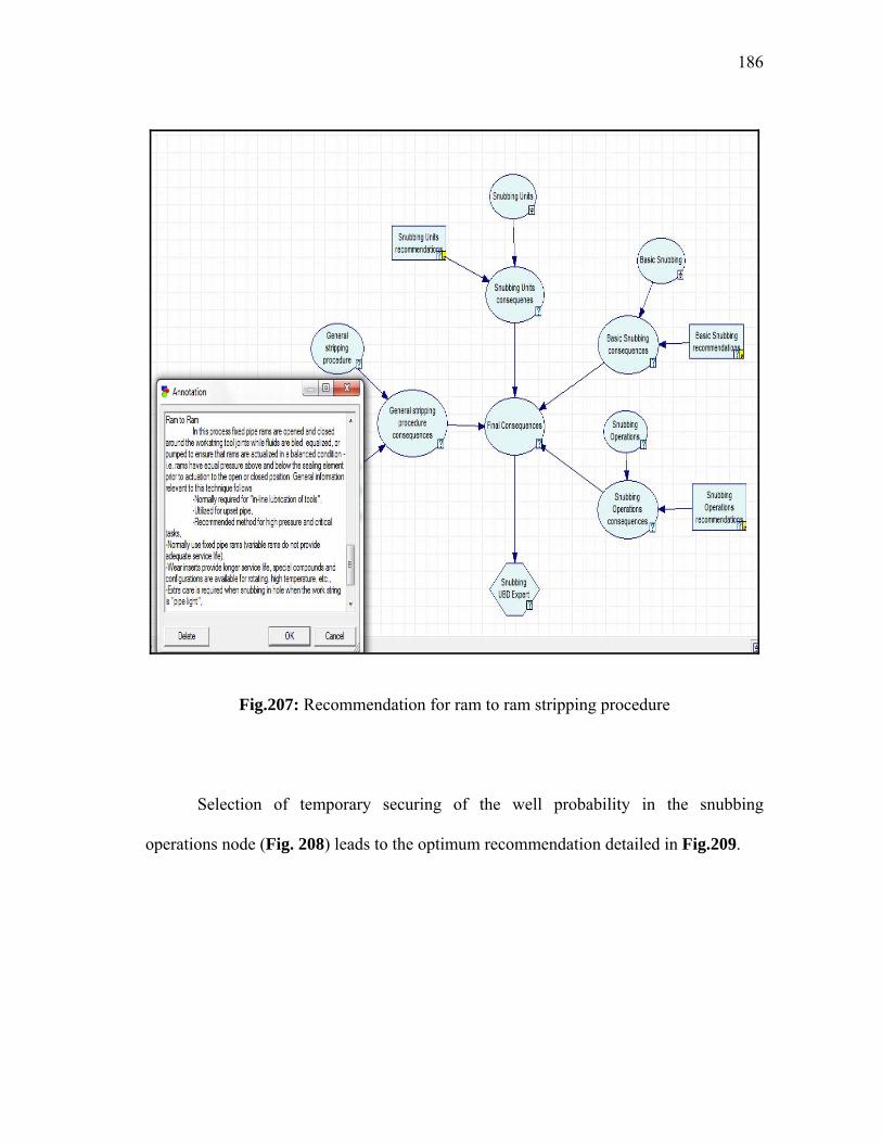
186

Fig.207: Recommendation for ram to ram stripping procedure

Selection of temporary securing of the well probability in the snubbing

operations node (Fig. 208) leads to the optimum recommendation detailed in Fig.209.

187

Fig.208: Selection of a snubbing operation (temporary securing of the well)

Fig.209: Recommendation for a snubbing operation (temporary securing of the well)

188

CHAPTER IX

CONCLUSIONS AND SUGGESTION FOR FUTURE WORK

The Bayesian approach was found suitable for designing expert system based on the

factors mentioned above. The model can work as a guide to aid drilling engineers and

scientists to design and execute optimum drilling fluids. Using this approach to build up

expert systems is more flexible than using flow charts. Updating flow charts is time

consuming and might require redesigning them again to be used by different experts or

in different fields. Using Bayesian Network allows us to update our industry practices by

updating the probabilities states mentioned in this research. Bayesian Network was used

to design models for well completion, drilling fluids, well control, cementing and

underbalanced drilling.

Literature review and completion experts’ opinions were used as evidence to

build a model using the proposed Bayesian Network. Variable nodes allow the user to

input desired well conditions that allows for generating the corresponding best

completion practices. Eighteen uncertainty nodes are defined for this model to determine

best practices in six decision nodes. The model is divided into six parts or decisions.

Each decision has uncertainties and consequences nodes.

189

The consequences node combines the uncertainty nodes where completion expert

opinions were used to assign and define the conditional probability distribution. The

model then calculates the optimum practices decision.

Literature review and drilling fluids experts’ opinions were used as evidence to

build the drilling fluid model. Variable nodes allow the user to input desired well

conditions that allows for generating the corresponding best drilling fluids practices.

Three uncertainty nodes are defined for this model to determine best practices in one

decision node (recommended drilling fluids). The model has one decision which has

uncertainties and one consequence node. The consequence node combines the

uncertainty nodes where drilling fluids’ expert opinions were used to assign and define

the conditional probability distribution. The model then calculates the recommended

drilling fluids decision.

The well control model is divided into three parts or decisions. Each decision has

uncertainties and consequences nodes. The consequences node combines the uncertainty

nodes where well control expert opinions were used to assign and define the conditional

probability distribution. The model then calculates the optimum practices decision. The

first part or decision provides the proposed circulation method decision based on the

kick details provided. The second part provides the user about the optimum

recommended practice based on the possible scenarios and operations in well control.

The third part provides the user with a quick check list for trouble shooting in case of

problems while controlling the well.

190

The cementing model has six uncertainty nodes (well type, objectives, bottom

hole static temperature, pumping time, drilling fluids, and consequences). This considers

three decision criteria (recommended cementing formulations, recommended spacers

formulations and recommended operational practices). The model is designed in a way

to give the user options to design well cementing and best practices effectively. The user

will select options that match his application from well type, bottom hole temperature or

required pumping time, objective and drilling fluid. Then the model (cementing expert

utility) will suggest optimum cement formulations, spacer formulations and operational

practices that fit the given well conditions.

Underbalanced drilling expert system here is combined into nine models as

follow:

o General approach to underbalanced drilling

o Flow underbalanced drilling

o Gaseated underbalanced drilling

o Foam underbalanced drilling

o Air and gas underbalanced drilling

o Mud cap drilling

o Underbalanced Liner Drilling Model

o Underbalanced Coil tube Model

o Snubbing and Stripping Model

Uncertainty nodes are defined for each model to determine best practices

decision nodes. The model is divided into several parts or decisions. Each decision has

191

uncertainties and consequences nodes. The consequences node combines the uncertainty

nodes where underbalanced drilling expert opinions were used to assign and define the

conditional probability distribution. The model then calculates the optimum practices

decision. Below are descriptions of the models.

The UBD General approach to underbalanced drilling model is divided into four

parts of uncertainty and decision nodes. The first part describes the formation to be

drilled underbalanced and the considerations required. The second part shows the

planning phases’ uncertainty and its corresponding recommendations. The third part

shows the equipments requirement uncertainty node or options and its corresponding

decision (equipment recommendations). The fourth part shows the operations planning

probability and its corresponding decisions

The flow UBD model is divided into three parts (tripping, connection and flow

drilling uncertainty and decision nodes). The gaseated UBD model is divided into four

parts (selection method benefits and challenges, requirements for general limits of gas

and fluid volume, operational concerns and challenges recommendations, and well kicks

recommendations). The foam model is divided into two parts (challenges and technical

limits with foam system and basic designs of foam systems). The air and gas model is

divided into four parts. The first part is rotary and hammers drilling probabilities and

recommendations. The second part is limits and challenges to gas drilling probabilities

and recommendations. The third part is rig requirements and recommendations. The

fourth part is gas drilling operations probabilities and recommendations. The mud cap

model is divided into three parts. The first part is background to mud cap drilling

192

probabilities and recommendations. The second part is drilling problems probabilities

and recommendations. The third part is floating mud cap drilling in depleted formation

probabilities and recommendations. The UBLD model is divided into three parts. The

first part is basic planning probabilities and recommendations. The second part is drilling

problems that can be solved and recommendations. The third part is limits and

challenges probabilities and recommendations. The underbalanced coil tube model is

divided into two parts. The first part is pre-planning probabilities and requirements. The

second part is drilling challenges probabilities and solutions. The snubbing and stripping

model is divided into four parts. The first part is basic snubbing probabilities and

recommendations. The second part is snubbing units’ probabilities and

recommendations. The third part is general stripping procedure and recommendations.

The fourth part is snubbing operations probabilities and its recommendations.

In case new practices or different experts’ opinions are presented then all we

need to do is simply change the states of probabilities. In case that the above model is

missing other factors then we can also update the model and its corresponding states of

probabilities. The flexibility of Bayesian Network in terms of updating the structure

model and its beliefs makes this method the first systematic approach to build experts

systems. This advisory system is intended to be a field guide for the drilling engineer or

rig supervisor.

193

9.1 Suggestion for future work

Future work can include designing a similar model using Bayesian Network for more

drilling operations such as managed pressure drilling practices. In addition, it will be of

interest to use the developed models in this research in the field for evaluation and

updating. For example, the drilling fluids model and the cementing model were

constructed using programs from Saudi Arabia. Programs from the USA can be used to

expand the practices due to different conditions such as higher temperature or shale gas

formation.

194

REFERENCES

Abbaspour, K., Matta, V., Huggenberger, P., and Johnso, C.A. 2000. A Contaminated

Site Investigation: Comparison of Information Gained from Geophysical

Measurements and Hydro-geological Modeling. Contaminant Hydrology 40: 365-

380.

Al-Kinani, A., Nunez, G., Stundner, M., Zangi, G., Iskandar, O., Mata, T., Cottone, S.,

and Cavero, J. 2009. Selection of Infill Drilling Locations Using Customized Type

Curves. Paper SPE 122186 presented at the SPE Latin American & Caribbean

Petroleum Engineering Conference, Cartagena, Columbia, 31 May- 3 June.

http://dx.doi.org/10.2118/122186-MS.

Al-Yami, A.S., Al-Arfaj, M.K., Nasr-El-Din, H.A., Jennings, S., Khafaji, A., Al-Ariani,

M., and Al-Humaidi, A. 2007. Development of New Retarder Systems to Mitigate

Differential Cement Setting in Long Deep Liners. Paper SPE/IADC 107538 presented

at the Middle East Drilling Technology Conference & Exhibition, Cairo, Egypt, 22-24

October. http://dx.doi.org/10.2118/107538-MS.

Al-Yami, A.S., Nasr-El-Din, H.A., Al-Saleh, S.H., Al-Humaidi, A.S., Al-Arfaj, M.K.,

Awang, M.Z., and Al-Mohanna, K.S. 2008. Lab Investigation of Oil Swelling

Elastomers for Smart Well. Paper OTC 19403 presented at the Offshore Technology

Conference, Houston, Texas, 5-8 May. http://dx.doi.org/10.2118/19403-MS.

Al-Yami, A.S. and Nasr-El-Din, H.A. 2009. Completion Fluids Challenges in Maximum

Reservoir Contact Wells. Paper SPE 121638 presented at the International

195

Symposium on Oilfield Chemistry, Woodlands, Texas, USA, 20-22 April.

http://dx.doi.org/10.2118/121638-MS.

Al-Yami, A.S., Nasr-El-Din, H.A., Al-Humaidi, A.S., Al-Arfaj, M.K., and Al-Saleh,

S.H. 2010a. Effect of HCl Acid and Brines on Water-Swelling Packers. SPE Drill &

Compl 25 (3): 322-327. SPE-114812-PA. http://dx.doi.org/10.2118/114812-PA.

Al-Yami, A.S., Schubert, J., Medina, C., and Ok-Youn, Y. 2010b. Drilling Expert

System for the Optimal Design and Execution of Successful Cementing Practices.

Paper IADC/SPE 135183 presented at the Asia Pacific Drilling Technology

Conference and Exhibition, Ho Chi Minh City, Vietnam, 1-3 November.

http://dx.doi.org/10.2118/135183-MS.

Al-Yami, A.S., Schubert, J., and Beck, G. 2011. Expert System for the Optimal Design

and Execution of Successful Completion Practices Using Artificial Bayesian

Intelligence. Paper SPE 143826 presented at the Brazil Offshore Conference and

Exhibition, Macaé, Brazil, 14-17 June. http://dx.doi.org/10.2118/143826-MS.

Al-Yami, A.S. and Schubert, J. 2012a. Drilling Fluids Consultation System:

Development and Field Applications. Paper SPE 152098 presented at the SPE

Western North American Regional Meeting, Bakersfield, California, USA, 19-23

March. http://dx.doi.org/10.2118/152098-MS.

Al-Yami, A.S. and Schubert, J. 2012b. Underbalanced Drilling Expert System

Development. Paper SPE 152101 presented at the SPE Western North American

Regional Meeting, Bakersfield, California, USA, 19-23 March.

http://dx.doi.org/10.2118/152101-MS.

196

Al-Yami, A.S. and Schubert, J. 2012c. Development of Optimum Well Control Practices

Using Artificial Bayesian Intelligence. Paper OTC 22882 presented at the Offshore

Technology Conference, Houston, Texas, USA, 30 April–3 May.

http://dx.doi.org/10.2118/22882-MS.

Al-Yami, A.S. and Schubert, J. 2012d. Guidelines for Optimum Underbalanced Drilling

Practices Using Artificial Bayesian Intelligence. Paper OTC 22883 presented at the

Offshore Technology Conference, Houston, Texas, USA, 30 April–3 May.

http://dx.doi.org/10.2118/22883-MS.

Brinkhorst, J.W. 1994. Optimization of Drilling Fluid and Clean-Up Operations in

Rogan South, Draugen Field, Norway. Presented at the Horizontal Well Technology

Forum, Aberdeen, 24-25January.

Carpenter, P., Nicholas, E., and Henrie, M. 2006. Bayesian Belief Networks for Pipeline

Leak Detection. Paper PSIG 0604 presented at the PSIG Annual Meeting,

Williamsburg, Virginia, 11-13 October. http://dx.doi.org/10.2118/0604-MS.

Dashevskiy, D., Dubinsky, V., and Macpherson, J.D. 1999. Application of Neural

Networks for Predictive Control in Drilling Dynamics. Paper SPE 56442 presented

at the SPE Annual Technical Conference and Exhibition, Houston, USA, 3-6

October. http://dx.doi.org/10.2118/56442-MS.

Downs, J.D. 1992. Formate Brines: New Solutions to Deep Slim Hole Drilling Fluid

Design Problems. Paper SPE 24973 presented at the European Petroleum

Conference, Cannes, France, 16-18 November. http://dx.doi.org/10.2118/24973-MS.

Ferraresi, M., Todini, E., and Vignoli, R. 1996. A Solution to the Inverse Problem in

197

Groundwater Hydrology Based on Kalman Filtering. Journal of Hydrology 175: 567-

581. http://dx.doi.org/10.1016/S0022-1694(96)80025-4.

Fjellheim, R., Herbert, M., Arild, O., Bisio, R., and Holo, O. 2010. Collaboration and

Decision Support in Geosteering. Paper SPE 128721 presented at the SPE Intelligent

Energy Conference and Exhibition, Utrecht, The Netherlands, 23-25 March.

http://dx.doi.org/10.2118/128721-MS.

Fink, J.K. 2002. Oil Field Chemicals. USA: Gulf Professional Publishing/Elsevier.

Garrouch, A.A. and Haitham, M.S. 2003. Using Fuzzy Logic for UBD Candidate

Selection. Paper IADC/SPE 81644 presented at the IADC/SPE Underbalanced

Technology Conference and Exhibition, Houston, Texas, U.S.A., 25-26 March.

http://dx.doi.org/10.2118/81644-MS.

Garrouch, A.A., Lababidi, H., and Abdullah, S. 2004. A Fuzzy Expert System for the

Completion of Multilateral Wells. Paper IADC/SPE 87963 presented at the

IADC/SPE Asia Pacific Drilling Technology Conference and Exhibition, Kuala

Lumpur, Malaysia, 13-15 September. http://dx.doi.org/10.2118/87963-MS.

Gelman, A., Carlin, J.B., Stern H.S. et al. 2003. Bayesian Data Analysis, second edition.

London. Chapman and Hall.

Ghabayen, S., McKee, M., and Kemblowski, M. 2006. Ionic and Isotopic Ratios for

Identification of Salinity Sources and Missing Data in the Gaza Aquifer. Journal of

Hydrology 318: 360-373. http://dx.doi.org/10.1016/j.jhydrol.2005.06.041.

Giese, M. and Bratvold, R.B. 2010. Probabilistic Modeling for Decision Support in

Integrated Operation. Paper SPE 127761 presented at the SPE Intelligent Energy

198

Conference and Exhibition, Utrecht, The Netherlands, 23-25 March.

http://dx.doi.org/10.2118/127761-MS.

Giese, M. and Bratvold, R. 2011. Probabilistic Modeling for Decision Support in

Integrated Operations. SPE Economics and Management 3 (3): 173-185. SPE-

127761-PA. http://dx.doi.org/10.2118/127761-PA.

Good, I. J. 1961a. A Causal Calculus (I). The British Journal for the Philosophy of

Science 11 (44): 305-318.

Good, I. J. 1961b. A Causal Calculus (II). The British Journal for the Philosophy of

Science 12 (45): 43-51.

GRØTTHEIM. O.E. 2005. Development and Assessment of Electronic Manual for Well

Control and Blowout Containment. MS Thesis, Texas A&M University, College

Station, Texas (August 2005).

Hayes-Roth, F. 1987. Expert Systems Applied to the Petroleum Industry Upstream

Portion. Paper SPE 22411 presented at the 12th World Petroleum Congress,

Houston, USA, 26 April – 1 May. http://dx.doi.org/10.2118/22411-MS.

Hill, A.D., Zhu, D., and Economides, M.J. 2008. Multilateral Wells, 35-50. Richardson,

Texas, SPE.

Howard, R.A. and Matheson, J.E. 1981. Influence Diagrams. The Principles and

Applications 2: 719-762.

Jonathan B. 2009. Well Completion Design. Amsterdam, The Netherlands: Elsevier. Kim, J.H. and Pearl, J. 1983. A Computational Model for Combined Causal and

Diagnostic Reasoning in Inference Systems. IJCAI83: 190-193.

199

Korb, K.B. and Nicholson, A.E. 2004. Bayesian Artificial Intelligence. London:

Chapman and Hall.

Kravis, S., Irrgang, R., Phatak, A., Martins, A., and Nakagawa, E. 2002. Drilling

Parameter Selection for Well Quality Enhancement in Deepwater Environments.

Paper SPE 77358 presented at the SPE Annual Technical Conference and Exhibition,

San Antonio, Texas, 29 September-2 October. http://dx.doi.org/10.2118/77358-MS.

Kulakofsky, D.S., Wu, F-L., Onan, D.D., and Wohleb, J.B. 1993. Development and

Application of a Knowledge-Based Expert System for Cement-Slurry Design. SPE

Comp App 5 (1): 21-25. SPE- 24417-PA. http://dx.doi.org/10.2118/24417-PA.

Lauritzen , S. L., and Spiegelhalter, D.J. 1988. Local Computations with Probabilities on

Graphical Structure and Their Application to Expert Systems. Journal of the Royal

Statistical Society Series B Methodological 50 (2): 157-224. ISBN: 1558601252.

Lee, C.-J. and Lee, K.J. 2005. Application of Bayesian network to the probabilistic risk

assessment of nuclear waste disposal. Reliability Engineering & System Safety 91(5):

515-532.

Lloyd, G.M., Bode, D.J., Nickens, H.V., and Varnado, S.G. 1990. Practical Applications

of Real-Time Expert Systems for Automatic Well Control. Paper SPE 19919

presented at the IADC/SPE Drilling Conference, Houston, Texas, USA, 27 February

- 2 March. http://dx.doi.org/10.2118/19919-MS.

McCaskill, J. and Bradford, W. 1972. Drilling Fluid System for Deep Drilling-An

Interrelated Approach. Paper SPE 3912 presented at the Deep Drilling Symposium,

Amarillo, Texas, 11-12 September. http://dx.doi.org/10.2118/3912-MS.

200

Pandey, V.J. and Osisanya, S.O. 2001. Development of an Expert System for Solids

Control in Drilling Fluids. J. Cdn. Pet. Tech. 40 (9): 50-59.

http://dx.doi.org/10.2118/01-09-05.

Pearl, J. 1988. Probabilistic Reasoning in Intelligent Systems: Networks of Plausible

Inference. San Francisco, California: Morgan Kaufmann Publishers.Inc.

Rajaieyamchee, M.A. and Bratvold, R.B. 2009. Real Time Decision Support in Drilling

Operations Using Bayesian Decision Networks. Paper SPE 124247 presented at the

SPE Annual Technical Conference and Exhibition, New Orleans, Louisiana, USA, 4-

7 October. http://dx.doi.org/10.2118/124247 -MS.

Rajaieyamchee, M.A. and Bratvold, R.B. 2010. A Decision Analytic Framework for

Autonomous Geosteering. Paper SPE 135416 presented at the SPE Annual Technical

Conference and Exhibition, Florence, Italy, 19-22 September.

http://dx.doi.org/10.2118/135416 -MS.

Rasheva, S. and Bratvold, R.B. 2011. A New and Improved Approach for Geological

Dependency Evaluation for Multiple-Prospect Exploration. Paper SPE 147062

presented at the Annual Technical Conference and Exhibition, Denver, Colorado,

USA, 30 October -2 November. http://dx.doi.org/10.2118/147062 -MS.

Rehm, B., Hebert, R., and Hebert, J. 1975. Practical Pressure Control. Tulsa,

Oklahoma: PennWell Publishing Company.

Roland, H., Suvaluck Ratanavani, C., Sevaphol le, M., Jonathan, N., Rossawan, C.,

Chawiwan, J., Siriwat, V., and Sawatdiwong, S. 2011. Water Production

Surveillance Workflow Using Neural Network and Bayesian Network Technology:

201

A Case Study for Bangkok North Field, Thailand. Paper IPTC 15015 presented at the

International Petroleum Technology Conference, Bangkok, Thailand, 7-9 February.

http://dx.doi.org/10.2118/15015 -MS.

Samuel, M., Marcinew, R., Al-Harbi, M., Samuel, E., Xiao, Z., Ezzat, A.M., Khamees,

S.A., Jarrett, C., Ginest, N.H., Bartko, K., Hembling, D., and Nasr-El-Din, H.A.

2003. A New Solids-Free Non-Damaging High Temperature Lost-Circulation Pill:

Development and First Field Applications. Paper SPE 81494 presented at the Middle

East Oil Technical Conference & Exhibition, Bahrain, 5-8 April.

http://dx.doi.org/10.2118/81494 -MS.

Sauer, C.W. and Landrum, W.R. 1985.Cementing-A Systematic Approach. JPT 37 (12):

2184-2196. SPE 11981-PA. http://dx.doi.org/10.2118/11981-PA.

Shadravan, A., Amani, M., Molinari, D., Politecnico, D.T., and Hugall, N.J. 2010.

Methods and Benefits of Knowledge Sharing in the Petroleum Industry. Paper SPE

137777 presented at the SPE Latin American & Caribbean Petroleum Engineering

Conference, Lima, Peru, 1-3 December. http://dx.doi.org/10.2118/137777-MS.

Smith, R.C.1984. Successful Primary Cementing Can Be a Reality. JPT 36 (11): 1851-

1858. SPE 13498-PA. http://dx.doi.org/10.2118/13498-PA.

Sousa, R. and Einstein, H.H. 2007. Risk Analysis for Tunneling Projects Using Bayesian

Networks. Paper presented at the 11th Congress of the International Society for Rock

Mechanics, Lisbon, Portugal. ISBN 979-0-415-45084-3.

202

Stoner, M.S. 2003. Fuzzy Logic for Directional Steering. Harts E&P,

http://www.makinhole.com/images/PDF/FuzzyLogic4DirectionalSteering.pdf

(downloaded 20 April 2012).

Wright, S. 1921. Correlation and Causation. Journal of Agricultural Research 20: 557-

585.

Wright, S. 1934. The Method of Path Coefficients. Annals of Mathematical Statistics 5

(3): 161-215.

Zerafat, M.M., Ayatollahi, S., Mehranbod, N., and Barzegari, D. 2011. Bayesian

Network Analysis as a Tool for Efficient EOR Screening. Paper SPE 143282

presented at the SPE Enhanced Oil Recovery Conference, Kuala Lumpur, Malaysia,

19-21 July. http://dx.doi.org/10.2118/143282-MS.

203

VITA

Name: Abdullah Saleh H. Alyami Address: Saudi ARAMCO, 9734 Dhahran, 31311, Saudi Arabia Email Address: abdullah.yami@aramcoservices.com Education: B.S., Chemistry, Florida Institute of Technology, Florida, 1998

M.S., Petroleum Engineering, King Fahd University of Petroleum & Minerals, Dhahran, Saudi Arabia. June, 2007 Ph.D., Petroleum Engineering, Texas A&M University, College Station, Texas, August 2012