USING ARTICULATED METROLOGY ARM TO … AND ALIGN OPTICAL SURFACES IN TERAHERTZ ASTRONOMY...
135
USING ARTICULATED METROLOGY ARM TO VERIFY AND ALIGN OPTICAL SURFACES IN TERAHERTZ ASTRONOMY APPLICATIONS by Mike Borden A Thesis Submitted to the Faculty of the COMMITTEE ON OPTICAL SCIENCES (GRADUATE) In Partial Fulfillment of the Requirements For the Degree of MASTER OF SCIENCE In the Graduate College THE UNIVERSITY OF ARIZONA 2011
Transcript of USING ARTICULATED METROLOGY ARM TO … AND ALIGN OPTICAL SURFACES IN TERAHERTZ ASTRONOMY...

USING ARTICULATED METROLOGY ARM TO VERIFY AND ALIGN OPTICAL SURFACES IN TERAHERTZ ASTRONOMY APPLICATIONS
by
Mike Borden
A Thesis Submitted to the Faculty of the
COMMITTEE ON OPTICAL SCIENCES (GRADUATE)
In Partial Fulfillment of the Requirements For the Degree of
MASTER OF SCIENCE
In the Graduate College
THE UNIVERSITY OF ARIZONA
2011
2
TABLE OF CONTENTS
List of Figures .................................................................................................................................4
List of Tables ..................................................................................................................................6
Abstract ...........................................................................................................................................7
1. Introduction ............................................................................................................................10
1.1. Verifying the Surface Figure of THz Optic ................................................................10
1.2. Aligning THz Optics ..................................................................................................11
1.3. Hypothesis...................................................................................................................13
2. Chapter 1: Project Background ..........................................................................................14
2.1. SuperCam ....................................................................................................................14
2.1.1. Tolerance Analysis of SuperCam Relay Optics...............................................20
2.2. FARO Arm..................................................................................................................25
2.2.1. FARO Arm Uncertainty Analysis ....................................................................27
2.3. Comparing Alignment Tolerances to Measurement Accuracy of FARO Arm ..........35
3. Chapter 2: Determining Surface Figure Accuracy and the Effect on Optical Performance ...........................................................................................................................36
3.1. Introduction .................................................................................................................36
3.2. Measuring an Optical Surface .....................................................................................38
3.3. Fitting Measured Dataset to Theoretical Surface Figure ...........................................41
3.3.1. Creating a CAD Model of the Theoretical Optical Surface .............................41
3.3.2. Initial Positioning of the FARO Coordinate Dataset .......................................48
3.3.3. Interpolating and Compensating for Probe Offset of FARO Data ..................51
3.3.4. Optimizing the Positioning of the FARO Coordinate Dataset .........................56
3.4. Analyzing the Surface Figure Results.........................................................................62
3.5. Determining Effect on Optical Performance of THz System .....................................65
3.5.1. Why Use Zernike Polynomials ........................................................................65
3.5.2. How to Generate Zernike Polynomial Coefficients .........................................67
3.5.3. Making Zernike Coefficients Compatible with ZEMAX ................................70
3.5.4. Generating Zernike Coefficients for Optimized FARO Dataset......................77
3.5.5. Entering Zernike Coefficients into ZEMAX ...................................................78

3
TABLE OF CONTENTS – Continued
3.5.6. Analyzing the Optical Performance Results ....................................................79
3.6. Considering Procedural Errors ....................................................................................83
4. Chapter 3: Aligning THz Optics ..........................................................................................85
4.1. Introduction .................................................................................................................85
4.2. Creating Reference Fiducials / Mechanical Reference for Optical Surface ...............87
4.2.1. Defining a Mechanical Reference ....................................................................88
4.3. Collecting Data Points ................................................................................................91
4.4. Transferring Reference Fiducial Coordinates from Measured to Theoretical Optical Surface .........................................................................................................................94
4.5. Modeling Mirrors and Reference Fiducials in SolidWorks ........................................96
4.5.1. Flat Mirrors ....................................................................................................102
4.6. Updating CAD Mirror Assembly with New Mirrors ................................................104
4.7. Using FARO Arm and Spatial Analyzer to Align THz Mirrors ...............................106
4.7.1. Aligning FARO Arm to First THz Mirror .....................................................109
4.7.2. Aligning Remaining Mirrors in System .........................................................113
4.8. Considering Procedural Alignment Errors................................................................116
5. Conclusions from Surface Characterization and Alignment Procedures ......................119
5.1. Verifying the Surface Figure of a THz Optic ...........................................................120
5.2. Aligning THz Optics .................................................................................................123
6. Appendix ...............................................................................................................................126

4
LIST OF FIGURES
Figure 1 - SuperCam reimaging optics for reducing f/# of SMT telescope ..................................15
Figure 2 - SuperCam relay optics, mirrors mounted in a rigid Optical Support Structure ...........15
Figure 3 - Mirror attached to kinematic mount via flexures .........................................................17
Figure 4 - SuperCam focal plane array .........................................................................................18
Figure 5 - Approximate beam placement on footprint of each mirror .........................................18
Figure 6 - ZEMAX layout of SuperCam optical assembly ..........................................................21
Figure 7 - Variations of measurement accuracy in regards to tilt .................................................23
Figure 8 - Probe Offset Diagram...................................................................................................26
Figure 9 - Visual representation of the uncertainty of a point measured with a CMM ...............27
Figure 10 - Triangle representing three points used in mirror alignment ....................................29
Figure 11 - Triangle translation as a result of deltas in the X direction ........................................30
Figure 12 - Y and Z triangle translations resulting from measurement uncertainty ....................30
Figure 13 - Triangle rotations resulting from measurement uncertainty .....................................31
Figure 14 – Author using FARO Arm to measure optical surface of mirror ...............................38
Figure 15 - Data points for ellipse using SolidWorks Equation Editor ........................................43
Figure 16 - The fully revolved ellipse in SolidWorks .................................................................44
Figure 17 - Rotation and translation to orient the center point of the mirror ................................45
Figure 18 - CAD model of re-oriented ellipse ..............................................................................46
Figure 19 - CAD Cutout of Ellipse ...............................................................................................47
Figure 20 - Original positioning of theoretical curve and FARO dataset ....................................48
Figure 21 - Top – FARO dataset roughly fit to theoretical curve. ................................................49
Figure 22 - Normals to the surface shown using MATLAB’s surface normal function ..............53
Figure 23 - : Probe offset corrected FARO data ..........................................................................55
Figure 24 - ASCII Import window which appears when data is imported into SA.......................57
Figure 25 - Point to Object Best-Fit Transformation pop up window ..........................................58
Figure 26 - Residual pop-up window which appears after a best-fit optimization in SA .............59
Figure 27 - Resulting best-fit transformation of FARO coordinate data to reference surface ......60
Figure 28 - Plot of fabrication error of M7 ...................................................................................62
Figure 29 - Explaining the observed error in SuperCam mirror M7 ............................................63

5
LIST OF FIGURES - Continued
Figure 30 - Plot of fabrication error of M4 ...................................................................................63
Figure 31 - First 10 Zernike functions with equations and aberrations ........................................65
Figure 32 - Normalized and circular FARO dataset of fabrication errors ....................................68
Figure 33 - Zernike coefficients, w/o and w/ normalization coefficient ......................................73
Figure 34 - ZEMAX window Extra Data Editor which is used to enter Zernike coefficients .....78
Figure 35 - OPD Fan of the optical performance of SuperCam ...................................................80
Figure 36 - Geometry of spherical FARO Arm probe in reference fiducial .................................88
Figure 37 - Machined fiducial with FARO Arm probe constrained within it...............................89
Figure 38 – Query Point To Surface Options Window .................................................................91
Figure 39 - Spatial Analyzer relationship report ...........................................................................93
Figure 40 - Measured optical surface optimized to theoretical CAD surface in SA ....................95
Figure 41 - Reference fiducial points inserted into CAD model of mirror ...................................96
Figure 42 - Lines to determine position of sides in relation to reference fiducial coordinates .....98
Figure 43 – The model of the CAD mirror being cut down to its correct side length ..................99
Figure 44 - SolidWorks model of mirror with correctly located fiducials ..................................101
Figure 45 - Completed CAD model of a flat mirror ...................................................................103
Figure 46 - .STEP model of updated mirrors correctly positioned in CAD mirror assembly ....105
Figure 47 - Mirror array CAD model and FARO Arm unreferenced to one another .................108
Figure 48 - Reference fiducial points created in SA ...................................................................109
Figure 49 - Transformation of actual measured points from mirror M7 to reference points ......111
Figure 50 - FARO Arm positioned in relation to mirror assembly. ............................................112
Figure 51 - Inter-Point Distance chart.........................................................................................114

6
LIST OF TABLES
Table 1 - Measurement uncertainties using the FARO Arm ........................................................33
Table 2 - RMS Error of surface fit on measured FARO data ......................................................52
Table 3 - Fabrication error of SuperCam powered mirrors, M4 and M7 ......................................64
Table 4 - Maximum residual error in relation to number of Zernike terms used .........................69
Table 5 - Comparison of first 10 Zernike modes ..........................................................................70
Table 6 - Normalization factors for MATLAB Zernike decomposition .......................................72
Table 7 - Template for rearranging Zernike order ........................................................................75
Table 8 – RMS WFE of optical system before and after as-built mirrors are entered ..................82
Table 9 - Distance between measured and ref points for final positioning of mirror M6 ...........114
7
Abstract
The field of Terahertz (THz) astronomy is a relatively new, but important and expanding area of
optics. As the THz region lies at the confluence of infrared and microwaves, observations at this
frequency utilize wavelengths that are much longer than visual spectrum optics. This provides
the unique opportunity that optical surfaces can be fabricated to looser machining tolerances. At
the same time, optical surfaces do not need to be well polished to be reflective at this frequency.
These characteristics can be used to fabricate THz optics that take less time to make and are less
expensive. The downside of this obvious advantage is that optical methods for characterizing
surfaces and aligning components cannot be used. There is thus a need for non-optical methods
of both characterizing the surface figure of THz optics and aligning THz optical components in a
system. It has been found that both of these procedures can be accomplished through the use of
an articulated metrology arm. The precision and accuracy of which is ideal for the metrology of
THz optics.
It has been determined that the surface figure of a THz optic can be characterized through the use
of an articulated metrology arm. The surface of the optic can be measured with the result being a
coordinate dataset representing that surface. In order to compare this measured surface to its
corresponding theoretical surface, some data processing must be completed. The measured data
is thus interpolated and an offset is incorporated into each data point to compensate for the radius
of the metrology probe. This corrected dataset is then best-fit to the theoretical surface. The
result of this transformation is a dataset describing the difference in surface figure between the
measured and theoretical surfaces. This difference in surface figure can then be analyzed to
determine how accurately a THz optic was fabricated. To take this one step further, the resulting
optical performance of a system can be determined based on the measured surfaces within this
8
system. This is done using Zernike polynomials to represent the difference between the
measured surface and the theoretical surface. Zernike polynomial coefficients are calculated for
this dataset and they are reentered into optical design software. The resulting optical
performance can then be determined. This procedure was used to characterize 2 off-axis conic
mirrors that are part of a relay optical system for a THz receiver called SuperCam. It was found
that neither mirror was made perfectly, but their overall effect on the optical performance of the
system was acceptable.
It has also been determined that the alignment of THz optics can be accomplished through the
use of an articulate metrology arm. The first challenge here is having a repeatable reference
point on each mirror to align to one another. The optical surface is not ideal for this as it is
unable to fully constrain the metrology arm probe. Thus, mechanical reference fiducials are
machined into the side of each mirror. By measuring the optical surface as well as these
reference fiducials with an articulated metrology arm, their positions in relation to the optical
surface can be determined. These fiducials thus become a reliable mechanical reference used in
mirror alignment. The fiducials are incorporated into a CAD model of each optic and a new
CAD model of the entire optical system is created. This updated CAD model is then imported
into Spatial Analyzer, which is a 3D coordinate management program where it will be used as a
theoretical reference for the location of each optic. The articulated metrology arm can then be
aligned to one of the THz optics and each corresponding optic will be aligned to the first. This
helps to minimize cumulative errors as each mirror in the system is aligned. The alignment is
done by measuring the reference fiducials with the metrology arm and then comparing the
measured coordinates to the theoretical positions of those fiducials. Adjustments to the
positioning of each mirror are then made and the process is repeated until the mirror is

9
adequately aligned. This procedure has been used to greatly simplify the alignment of a complex
optical system: the SuperCam relay optics. Additionally, calculations were completed which
found that the measurement accuracy of the metrology arm was well within the alignment
tolerance limit required by the optical system. While the methods presented here were
developed for THz optics they potentially represent a time saving step in the alignment of
more conventional optical systems.

10
1. Introduction
Though optics in the THz frequency are similar in many ways to shorter wavelength optics, there
are a number of differences that make them unique. Gaussian beam propagation is used rather
than traditional geometric ray tracing. Optical surface figure and alignment tolerances are more
forgiving at sub-millimeter wavelengths. Mirrors for THz optical systems do not need to be well
polished to be reflective at these frequencies. At the same time, there are similarities that are
common in optical systems regardless of wavelength. Optical surfaces must be fabricated to an
acceptable accuracy to maintain the desired optical performance. Optical components in a
system must be aligned to an acceptable tolerance in relation to one another, again to maintain
the desired optical performance. Though these are common challenges in any optical system, it
is the unique characteristics of THz optics that allow for, and even require, a different approach.
1.1. Verifying the Surface Figure of a THz Optic
The first of these challenges is in regards to verifying the surface figure of a fabricated THz
optic. As mentioned, the tolerances for fabricating a THz optical surface are indeed more
forgiving than shorter wavelength optics. In addition, the surface does not need to be polished to
the optical quality it would require for wavelengths in the visual spectrum to reflect THz beams.
For both of these reasons, THz optics can be made at less cost than a high precision, finely
polished optical surface. This obvious advantage comes with the inherent disadvantage that the
machining methods used are more likely to introduce undesired errors. Pair this with requiring a
challenging optical surface, such as off-axis conics, and there can be genuine concern about how
well these surfaces have been made. Although not needing an optical quality surface for these
mirrors is convenient, it also comes with inherent disadvantages. Optical methods for
determining the surface figure of an optic, such as with an interferometer or Point Source

11
Microscope (PSM), will not work if the surface is not adequately reflective. A fabricated optic
can in turn be polished to allow the use of these optical methods, but undesired effects to the
surface figure can be the result. For these reasons, there is a need for a method of determining
the surface figure of an inexpensively made THz optic that has not been polished to optical
quality. Two significant questions that could be answered by such a method are:
• How accurately was the optical surface fabricated?
• How do the fabricated optical surfaces affect the optical performance of the system?
To answer these questions, Chapter 2 of this thesis will discuss a surface figure measuring
technique that utilizes an articulated metrology arm. The metrology arm will be used to measure
the optical surface. With some processing of this coordinate data, the measured surface figure
can be determined and compared with the desired surface figure. Finally, this measured optical
surface can be reentered into optical design software to determine its effect on the performance
of the entire optical system. Though this particular technique can be performed with any
coordinate measuring machine (CMM), an articulated arm provides advantages that will be
utilized later during mirror alignment.
1.2. Aligning THz Optics
Aligning THz optics is subject to the same disadvantages discussed when verifying their surface
figure. Again, their surfaces may not be polished to optical quality which makes using optical
alignment instruments, such as a laser tracker or PSM, difficult or impossible. Traditional
alignment techniques for THz optics start by using non-stretching wire to provide the correct
spacing between optics. If the THz optics are polished, at least in the center of the optic then a
laser is mounted along the optical axis to help position the mirrors. These provide a crude

12
alignment. Finally, the THz receiver is used to do beam mapping with hot and cold loads. This
can provide an excellent final alignment but doing the mirror alignment with this method can be
difficult. Once the mirrors are position, beams can be mapped to determine if the optics are
indeed aligned. If they are not, as they most certainly won’t be to begin with, some investigation
in regards to what optic in the system needs to be moved and by how much needs to be done.
This can be very challenging and time consuming. There is thus a need for a non-optical
alignment technique that provides accurate positioning of each THz optic. If such a procedure
could be used to initially align each mirror, then beam mapping can be done to make final, small
adjustments, if they are needed at all. The questions that could be answered by such a non-
optical alignment technique are:
• How accurately is each optic aligned?
• Is this alignment adequate for the performance of this system?
To answer these questions, Chapter 3 of this thesis will discuss an alignment technique that
utilizes an articulated metrology arm. But simply measuring optical surfaces to reference to one
another provides challenges of its own. First off, an erroneous surface makes a poor reference
surface for mirror alignment. Secondly, it is difficult to constrain the probe of an articulated
metrology arm on an optical surface. This makes point to point relationships between optics
impossible. Thus, a technique has been developed to provide mechanical reference points on
each mirror that are related to the optical surface and can be used for mirror alignment.

13
1.3. Hypothesis
Using an articulated metrology arm, coordinate data processing, and optical design software, the
surface figure of non-reflective THz optics can be verified and its resulting effect on the optical
system can be determined.
Through the use of an articulated metrology arm and mechanical reference fiducials, non-
reflective THz optics can be aligned within the alignment tolerances required of the system.

14
2. Chapter 1: Project Background 2.1. SuperCam
The challenges of verifying and aligning THz optics were brought to light by the SuperCam
project. SuperCam is a 64 pixel imaging spectrometer being developed by Dr. Chris Walker and
the Steward Observatory Radio Astronomy Laboratory (SORAL). Observing at 350 GHz, or
857um, SuperCam will be used to answer fundamental questions about the physics and
chemistry of molecular clouds in the galaxy and their direct relation to star and planet formation.
When completed, SuperCam will be installed in the Submillimeter Telescope (SMT) on Mount
Graham near Safford, AZ. The SMT is one of the most accurate large submillimeter telescopes
currently in operation. Its location on Mt. Graham at 10,500’ elevation also provides sufficient
weather for observing.
In order to integrate SuperCam with the SMT, a system of re-imaging optics were found to be
necessary. The existing secondary mirror of the SMT provides an f/13.8 beam at its focus.
Since the physical separation between array elements in the instrument focal plane scales as 2fλ,
lower f/#’s serve to reduce the overall size of the instrument. Thus, the reimaging optics are
used to reduce the f/# of the telescope to f/5. In addition, these reimaging optics are used to
make the optical system telecentric in image space and also provides adjustment of the plate
scale. These reimaging optics, which are located in the apex room of the telescope, are shown
below in Figures 1 and 2. (Groppi)
15
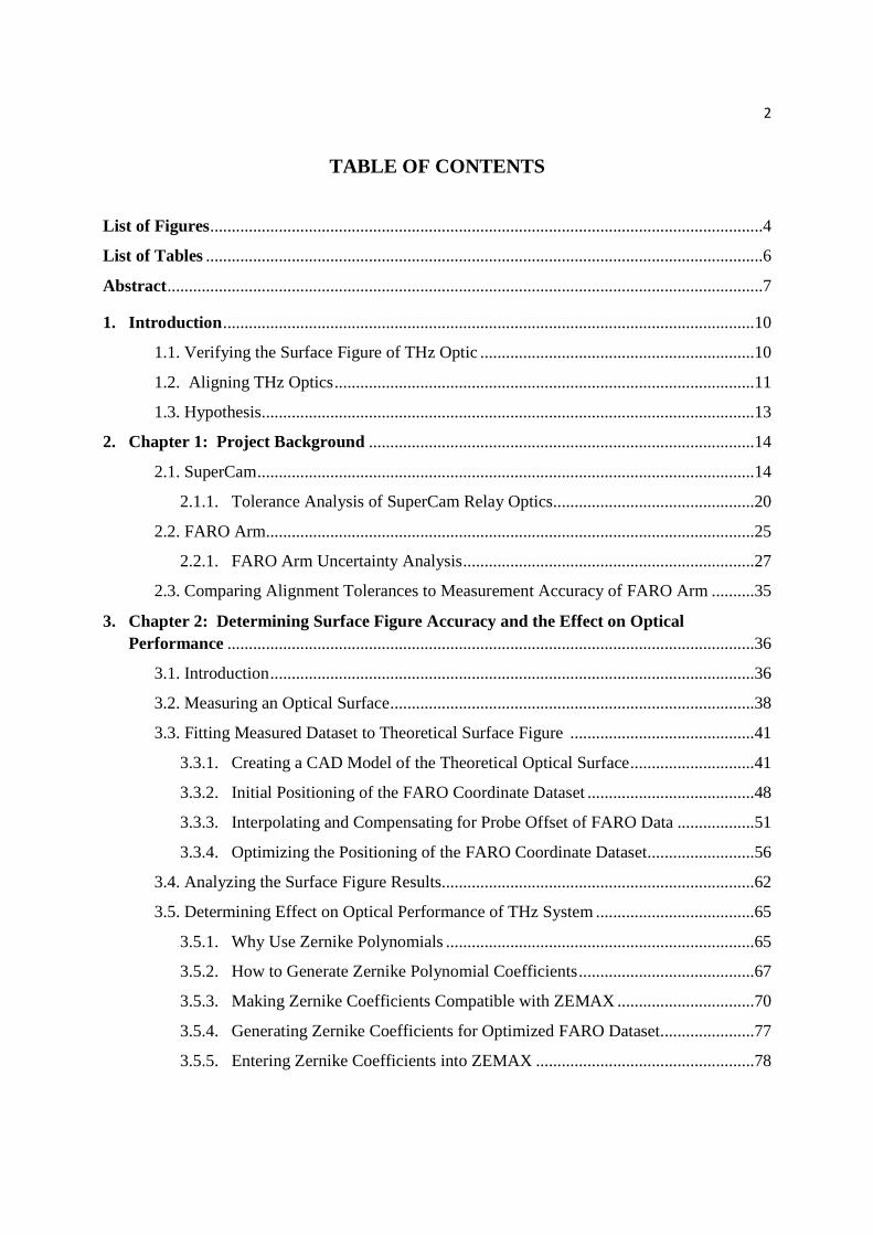
Figure 1: SuperCam reimaging optics for reducing f/# of SMT telescope. Left – Top view showing the beam bundles (in red) passing through the SMT primary mirror and into the apex
room. Right – SuperCam relay optics seen within apex room. (Groppi)
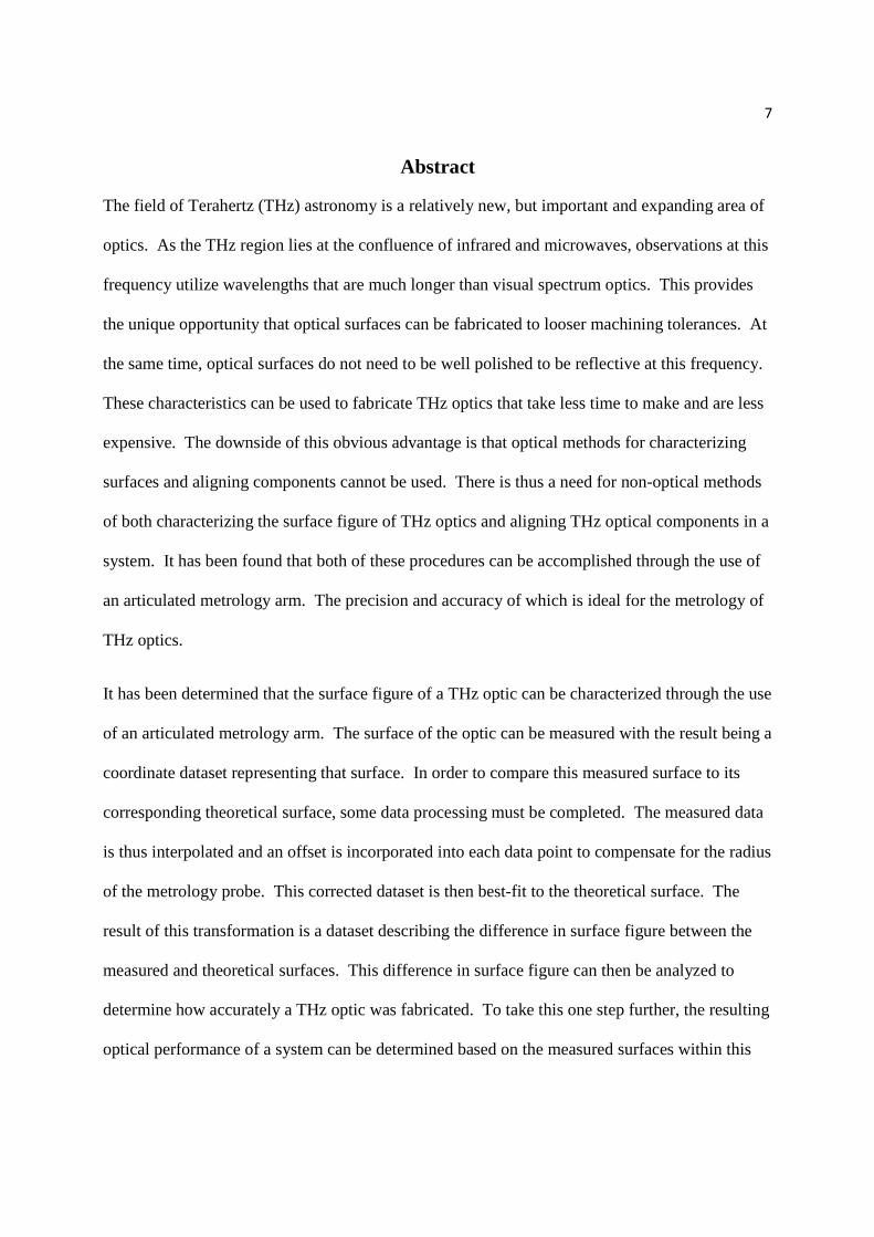
Figure 2: SuperCam relay optics, which consist of 7 mirrors mounted in a rigid Optical Support Structure (OSS)
16
The relay optics shown in Figures 1 and 2 consists of 5 flat mirrors, 1 off-axis parabola, and 1
off-axis ellipse. All but one flat mirror are mounted within a single modular frame, the Optical
Support Structure (OSS). The intention is to align and test the reimaging optics off the telescope
and in the lab. It will then be integrated into the telescope with only minor alignment within the
relay optics necessary.
Each mirror in the relay optics system has been directly CNC machined from aluminum. After
the mirrors were fabricated and returned to SORAL, a great deal of time was spent hand
polishing each mirror. This was done because the original intention was to use a laser to align
each mirror in the system. Flexures were then bonded to the back of each mirror. This is to
minimize mirror deformation resulting from being rigidly attached to mirror mounts. The mirror
mounts used are custom designed and fabricated kinematic optical mounts. Each kinematic
mount employs two computer controlled stepper motors that allow for motion in the tip and tilt
directions. These mirror mounts are then installed within the OSS, which is made from steel
Unistrut frame. The one flat mirror that is not installed in the OSS is used as a pickoff mirror for
the telescope beam. This mirror is mounted on a sliding stage and intercepts the beam from the
telescope tertiary and directs it into the SuperCam OSS. The mounted mirror design is shown
below in Figure 3.
17
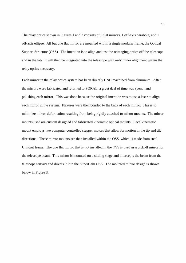
Figure 3: Mirror attached to kinematic mount via flexures. The whole structure is then mounted to the OSS.
SuperCam’s focal plane array helps to dictate the placement of beams on the surface of each
mirror. As mentioned, SuperCam utilizes a 64 pixel focal plane array. This can be seen in
Figure 4.

18
Figure 4: SuperCam focal plane array. Left – Full focal plane array not yet installed in SuperCam. Note the 64 feedhorns machined into the array. Right – Half of focal plane array
installed in SuperCam.
Thus, placement of the beams from each pixel is shown below in Figure 5. This general beam
placement holds true for each mirror in the relay optics system.
Figure 5: Approximate beam placement on footprint of each mirror

19
Based on the required beam placement on each mirror as shown in Figure 5, it can be seen that
vignetting light at any point in the relay optics system is unacceptable. The result would be the
loss of pixels near the edges of the focal plane array. This reality helps to dictate the required
alignment tolerances of the SuperCam relay optics.

20
2.1.1. Tolerance Analysis of SuperCam Relay Optics
The mirrors in the SuperCam optical system must be aligned to a certain tolerance for the
resulting optical performance to be acceptable. Thus a tolerance analysis must be completed to
determine the alignment precision necessary for each of the 6 degrees of freedom: translations in
X, Y, and Z, and rotations in θ, φ, and α. As the FARO Arm is the alignment instrument, its
measurement accuracy must be compared to the required tolerances to determine if it will be an
acceptable alignment instrument.
A figure of merit to be used in this tolerance analysis is the wavefront error at the focal plane
array of SuperCam. The wavefront error is an excellent figure of merit because it represents how
well a beam has focused after passing through the optical system. Based on experience with
optical systems at this wavelength, a wavefront error of �� is considered the total allowable error
in this system. This amount of wavefront error represents the point in which the system is
approximately diffraction limited. It is thus important that the wavefront error derived from
mirror alignment be well below this allowable error. As surface figure errors are also expected,
this will add to the overall wavefront error of the system. The layout of the optical system is
shown below in Figure 6.
21
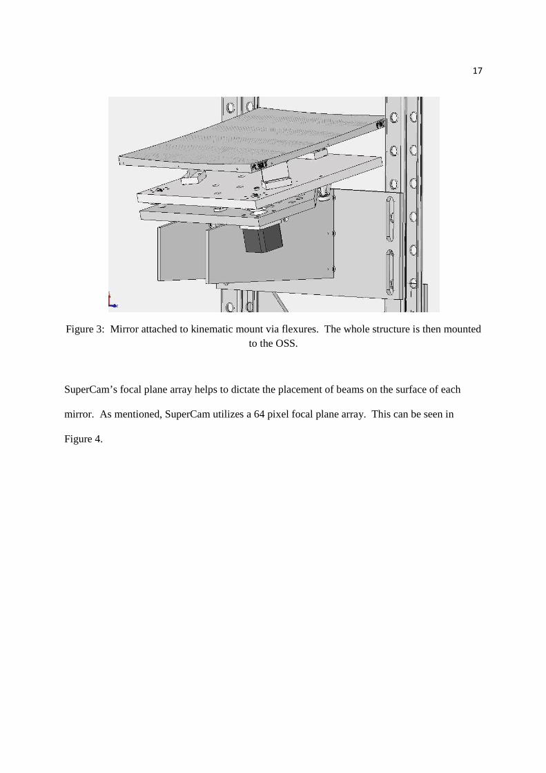
Figure 6: ZEMAX layout of SuperCam optical assembly
A Monte Carlo tolerancing analysis will be performed in ZEMAX to determine the necessary
alignment tolerances of the system. The Monte Carlo analysis allows the user to declare the
figure of merit to be used for the analysis as well as the acceptable amount of error for that figure
of merit. In this case, a wavefront error of ��� is entered, a value which leaves significant room
for surface figure related wavefront error. In regards to the Mode of the Monte Carlo analysis,
the Inverse Limit is selected. This allows the user to enter the permissible change of criterion (ie
allowable positioning error) and the change in wavefront error is determined.
22
The degrees of freedom that are affected by errors in mirror positioning are to be entered into the
Monte Carlo analysis. As mentioned, these are errors in translations in X, Y, and Z, and
rotations in θ, φ, and α. For translations in Z, which is considered thickness in ZEMAX, the
operator used is TTHI. For translations in X and Y, TEDX and TEDY are used, respectively. For
rotations in θ, φ, and α, the operators are TETX, TETY, and TETZ, respectively. For the
translations, the units are in millimeters will the rotations are in degrees. The maximum and
minimum position and rotation errors are then entered. This process is done with trial and error.
Again, previous experience can help determine a starting place. Once these maximum and
minimum values are entered, the number of Monte Carlo iterations is selected and the analysis is
run. The result is a data file which contains information about how much the wavefront error
changes based on each individual tolerance as well as the estimated RMS wavefront error of the
system. The worst offenders are also listed. Based on this feedback, the tolerances can be
adjusted. The goal is to provide tolerances which are as loose as possible while still maintaining
the optical performance desired. Looser tolerances allow for less positional accuracy required
for aligning the mirrors.
Based on trial and error, the acceptable tolerances are:
Thickness / Piston: 1mm
Translation in X and Y: 1mm
Rotation in θ and φ: 0.1 deg
Rotation in α: 0.5 deg
These alignment tolerances produce a resulting RMS wavefront error of about ���. These
tolerance present only a small amount of additional wavefront error, as the original RMS
wavefront error of the system was ���.
23
As expected, the worst offending tolerances were the tip and tilt rotations. As the path length
through the system is quite long, a small alignment error in tip or tilt can quickly result in a
degradation in wavefront error or worse yet, the vignetting of beams near the edges of the
mirrors. It is this vignetting concern that does not allow for the tip and tilt tolerances to be
looser. This would have been ideal as the tip and tilt tolerances are quite tight and the wavefront
error is incredibly conservative.
The translation tolerancing is easily compared to the measurement accuracies of the FARO Arm.
One millimeter of position accuracy is easily achieved with the FARO Arm. In fact, according
to the measurement uncertainty analysis, the FARO Arm can measure with less than 10um of
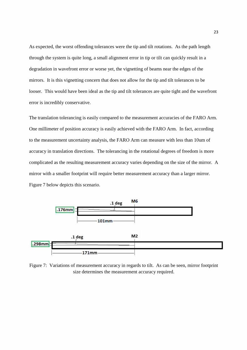
accuracy in translation directions. The tolerancing in the rotational degrees of freedom is more
complicated as the resulting measurement accuracy varies depending on the size of the mirror. A
mirror with a smaller footprint will require better measurement accuracy than a larger mirror.
Figure 7 below depicts this scenario.
Figure 7: Variations of measurement accuracy in regards to tilt. As can be seen, mirror footprint size determines the measurement accuracy required.

24
As can be seen in Figure 7, a smaller mirror requires better measurement accuracy. To
determine if the FARO Arm is capable of achieving this accuracy, the smallest mirror (M6) is
used as an example. This mirror requires 0.1 degrees of tip and tilt, which amounts to .176mm
of measurement accuracy in the translational direction.
A closer look at the measurement accuracy the FARO Arm is capable is necessary to determine
if the tolerances required by M6 can be achieved.

25
2.2. FARO Arm
In order to analyze the surface figure of an optic, a dataset of coordinates must first be generated.
To accomplish this, a Coordinate Measuring Machine (CMM) is typically used. There are a
wide range of CMMs on the market but in this case, an articulated metrology arm will be used.
The particular Arm being used is a FARO Quantum 8’ Arm. The advantages of using the FARO
Arm include:
• Large measurement range: it can take measurements within a range of 8’ in diameter.
This provides a large enough range that every mirror within the system can be
measured without moving the arm.
• 3-dimensional measuring: probe can measure surfaces from any angle because of
multi-jointed arm. This allows for measurements of not only the surface of each
mirror, but also reference points on the sides.
• Excellent measurement accuracy: 20um per point or 28um between points. An
uncertainty analysis will be performed to determine if this measurement accuracy is
adequate in this application.
• Portable: A portable arm is necessary as some alignment of the SuperCam relay
optics will be necessary while performing the installation in the SMT apex room.
This is not to say that the FARO Arm is the only articulated metrology arm that can be used.
Because of the aforementioned advantages and its availability, the FARO Arm was used in this
application.
It should be noted that data points are taken at the center of FARO Arm’s probe, rather than at its
surface. This concept is shown in Figure 8 below.

26
Figure 8: Probe Offset Diagram
To compensate for this, an offset the size of the probe radius must be incorporated into each
X,Y,Z coordinate taken by the FARO Arm. The probe that was used in this example has a radius
of 1.5mm. Thus, a 1.5mm offset must be added or subtracted to the data in the direction normal
to the surface at each point. This will be done using a MATLAB function which calculates a
vector normal to the surface. This vector is then used to offset the 1.5mm probe radius.
Accounting for this probe offset will be done numerous times throughout the following
procedures.
The software that the FARO Arm runs on is Spatial Analyzer (SA). SA is a 3D metrology
software platform that is used for interfacing with dimensional measurement systems. In this
case, SA is used to record the coordinates of the points measured by the FARO Arm. It will also
be used to best-fit transform measured datasets to theoretical optical surfaces.
To determine if the FARO Arm provides adequate measurement accuracy for this THz
application, an uncertainty analysis must be performed.

27
2.2.1. FARO Arm Uncertainty Analysis
There is a limit to the measurement accuracy which can be achieved with a CMM. This can be
seen when a fully constrained point is measured repeatedly. The returned coordinates will show
a slight deviation in X, Y, and Z each time the point is measured. In an ideal world, the CMM
would return the exact same coordinates for the point every time it is measured. In reality, there
is some uncertainty to every measurement that is taken. The uncertainty of a measured point can
be thought of as a cloud of points surrounding the one which was recorded. This cloud
represents the possible positions that could be recorded when the point is taken. This is shown
below in Figure 9.
Figure 9: Visual representation of the uncertainty of a point measured with a CMM. Each tiny dot represents a possible position for the point that was measured. This image was taken from a
Spatial Analyzer uncertainty analysis of points measured by a FARO Arm.
These point clouds are the result of the CMM having reached its smallest increment of
measurement. In the case of the FARO Arm, it is the resolution of the position encoders in each
joint which determine this minimum increment. This is commonly the case with CMMs.
FARO Arm is unique in that each of its joints has an encoder which is used to determine the

28
position of the probe. The output of each encoder in combination is used to determine the final
probe position. It should be noted that not every combination of encoder positions will produce
the same measurement accuracy. This means that depending on which encoders are referenced
(which joints are bent) and by how much, the uncertainty in a measurement can vary. Thus, the
point cloud shown above in Figure 9 is not perfectly spherical. A further analysis of this
phenomenon would be useful to determine how to achieve the most accurate measurements
when using the FARO Arm. Regardless, the following uncertainty calculations will be
completed using the mathematical simplification that the point cloud is spherical.
As each measured point has some inherent uncertainty, the points used in the mirror alignment
process must account for this uncertainty. There are three reference points that will be measured
for each mirror during the alignment. When measurement uncertainty is incorporated into each
of these three points, errors can be introduced. The uncertainty in a measured point can result in
mirror positioning errors in X, Y, and Z, as well as mirror rotations in θx, θy, and θz. These errors
thus represent the limit to the position and rotation accuracy of each mirror that can be achieved
with the FARO Arm.
The uncertainty errors of each degree of freedom can be calculated for each mirror. To
accomplish this, the first step is to populate the following matrix. These values are calculated
based on the triangular geometry that results from using three measured reference fiducial points.
This matrix will be identified as matrix [A].

29
[A] =
� ��
��
� �
� ��
��
�� ���
��� �
�� ��
�� ���
���
�� ���
��� �
�� ��
�� ���
���
��� ����
���� ��
��� ���
��� ����
����
��� ����
���� ��
��� ���
��� ����
����
��� ����
���� ��
��� ���
��� ����
����
The calculations for populating Matrix [A] are shown below. Figure 10 defines how the three
points are labeled and how the axes and rotations are defined.
Figure 10: The above triangle represents the three points that are used in mirror alignment. The diagram defines how the points, axes, and rotations are labeled.
Figure 11 below shows the resulting translation of the triangle in the X direction as a function of
the uncertainty in the coordinate of X1. The resulting partial derivates for each of the three
points are also shown.

30
Figure 11: Triangle translation as a result of deltas in the X direction resulting from uncertainty in measurements.
The delta shown in Figure 11 represents the possible deviation from the actual point that results
from measurement uncertainty. In this case, only the deviation in along the X-axis is considered.
The partial derivative variables describe the triangle translation in the X direction as a result of
the x-axis uncertainty of each measured point.
Next, the translations in the Y and Z directions are calculated. These are shown below in Figure
12.
Figure 12: Y and Z triangle translations resulting from measurement uncertainty in those directions

31
Next the rotations that can result from measurement uncertainty are calculated. These are shown
below in Figure 13.
Figure 13: Triangle rotations resulting from measurement uncertainty
All of the remaining partial derivative variables are 0 in this case. Once all of these values are
determined, then they can be entered into their respective positions in matrix [A]. This
completed matrix is shown below.

32
[A] =
13 0 0 13
0 0 13 0 0
0 13 0 0 13
0 0 13 0
0 0 13 0 0 13
0 0 13
0 0 0 0 0 0 0 0 −1��
0 0 −12�� 0 0 12�
0 0 0
0 13�� 0 0 13�
0 −13�� 0 0
Another matrix must be created representing the magnitude of the uncertainty errors. This will
be called matrix [B] and it is shown below.
[B] =
��� ��� ��� �� �� �� ��� ��� ���
With the FARO Arm, the most accurate measurement that can be taken repeatedly in a 3D
environment is 28um. The values for ��, ��, and �� for each point are thus calculated as
follows.
. 028�� = !�� + ∆� + ∆�

33
Considering the approximation that the uncertainty point cloud is spherical, ∆�, ∆�, and ∆� are
all equal. Thus, the resulting measurement uncertainty in one direction is 0.016mm or 16um.
This value is input for every variable in matrix [B].
To calculate the final uncertainty of each degree of freedom, the following equation must then be
used. The value of ∆X will be used as an example.
∆� = $∑ ['(), +, ∗ .(), +,] 012� Equation 1
This equation with actual variables entered into it is shown below.
∆� = 34( � ∗ ���, + ( �� ∗ ���, + ⋯ + ( �� ∗ ���,
This calculation is performed 6 times for each degree of freedom of the measured triangle.
It should be noted that the values for ��, ,� need to be defined before uncertainty values can be
calculated. These values depend on which mirror is being measured and which three fiducials
were used as an alignment reference. For some example uncertainties, three fiducials on the
smallest mirror (M6) were chosen. A smaller mirror means reference fiducials which are closer
together which produces larger rotational uncertainties. The resulting uncertainties are shown
below in Table 1.
Table 1: Measurement uncertainties using the FARO Arm
X 9.33um Y 9.33um Z 9.33um �� .0044 deg �� .0065 deg �� .0046 deg

34
These uncertainty values define the limitations in measurement accuracy of the FARO Arm. As
these uncertainties are inherent in the measurements taken by the FARO Arm, there is no
escaping them. They must be compared to the tolerance analysis of the optical system being
aligned to determine if the measurement accuracy of the FARO Arm is adequate.

35
2.3. Comparing Alignment Tolerances to Measurement Accuracy of FARO Arm
Based on the required alignment tolerances for the SuperCam relay optics, it was determined that
the smallest mirror, M6 required 0.1 degrees of tip and tilt tolerance and .176mm of
measurement accuracy in the translational direction. After performing an uncertainty analysis, it
has been determined that a measurement accuracy of 0.0065 degrees and a translational
measurement accuracy of less than 10um is achievable using the FARO Arm.
The final conclusion of this tolerance analysis paired with the uncertainty analysis is that the
FARO Arm has a measurement accuracy which is capable of adequately positioning the mirrors
in the SuperCam relay optics system.

36
3. Chapter 2: Determining Surface Figure Accuracy and the Effect on Optical Performance
3.1. Introduction
A great deal of effort goes into the design and fabrication of an optical surface. Rightfully so as
the performance of an optical system is highly dependent upon the accuracy in which a surface
figure has been fabricated. In applications where a commercial optic can be used, the accuracy
of its surface figure is often well known: companies will have determined the surface figure
accuracy which their fabrication process can routinely produce. On the other hand, in
applications where custom optical surfaces are required, the accuracy of a surface figure often
needs to be determined by the user of the optic. This can be an intensive process requiring the
time of highly trained individuals and the use of expensive metrology equipment. The process
can thus be expensive. An additional challenge remains even after an optical surface has been
characterized: how will the surface figure of the measured optic impact the overall performance
of an optical system? A fabricated optical surface will never be perfect; machining processes
and if necessary, mechanical polishing, can both incorporate error into the surface. These
problems are amplified when an optic is fabricated at low cost. Thus, having a way to
characterize the performance of a system with the existing optical components can be valuable.
Optical components in THz astronomy applications are no different. Though wavelengths are
long in relation to the visual spectrum and Gaussian beam propagation is used rather than
geometric ray tracing, surface figure remains critical. Fortunately, in THz astronomy, the longer
wavelengths are more forgiving in regards to the required surface figure accuracy. This is
because errors are observed as fractions of wavelengths. A wavefront error of λ/20 for λ = 1mm
represents only 50um while a shorter wavelength of λ = .5um represents .025um. This is a
considerable difference in fabrication and alignment tolerances. With this in mind, the mirrors

37
for the SuperCam optical array were fabricated and polished at low cost. Each of the 7 mirrors
were machined out of aluminum by a machine shop that was capable of, but not specializing in
machining optical surfaces. Once the mirrors were returned to SORAL, they were mechanically
polished by hand. After making the mirrors in this way, it became all the more valuable to
characterize the final surface figure of each mirror. In the case of the flat mirrors, the fabrication
process, grinding, is a well understood and proven method for generating a flat surface. In this
particular application, the flat mirrors from the SuperCam relay optics were fabricated and tested
for flatness by the manufacturer. The 2 powered mirrors in the system, being complex surfaces,
were made using a less proven fabrication process. This led to greater concerns about their
surface figure. Thus, the following procedure emphasizes characterizing curved optical surfaces
for THz applications.

38
3.2. Measuring an Optical Surface
Before coordinates of the optical surface can be taken, the optic itself must be positioned so that
it is stable during measurement. The probe must touch the surface of the optic to take
measurements so if it is even slightly unstable and
the optic moves when touched, it can render an
entire dataset useless. Unless the mirror or lens
being measured is rotationally symmetric then the
rotation of the mirror should be noted. Knowing
where the first measurements were taken and how
the optic is oriented will be useful later.
It should be noted at this point that the FARO Arm
is simple to calibrate before use. A mechanical cone
shaped reference is used to run through the range of
motion of the arm’s encoders. A calibration should
be done occasionally, but is not necessary every
time the arm is used as it remains calibrated between
uses.
Once the optic is mounted well and its orientation is known, the FARO Arm should be used to
designate the coordinate system for the measurements. This can be done using 3 intersecting
reference planes and the Spatial Analyzer function Locate which is found under the Instrument
drop bar. In the case of the flat mirrors, the reference plane should be two intersecting sides and
the flat optical surface. Creating a coordinate system from these planes will designate that corner

39
as the origin with coordinates (0,0,0). For curved mirrors, the reference planes should be two
intersecting sides and the flat table the mirror is sitting on. The origin generated from the
intersection of these 3 planes is a bit less useful but it still is an improvement over having a
completely arbitrary coordinate system. Designating the origin to be near the measured surface
will make the data easier to use in future steps.
At this point, taking measurements with the FARO Arm can now begin. For mirrors, only one
optical surface needs to be measured. For lenses, the lens should be mounted in a way that
allows for both surfaces to be measured without repositioning. In either case, a large number of
points should be taken when measuring the optical surface. A few hundred points were taken for
each mirror in this example. Points can be measured each time the probe trigger is pushed or in a
continuous stream called the Drag method. The Drag method allows the probe to be dragged
along a surface while taking points at a set interval. It allows the user to collect a large number
of points while keeping the probe in constant contact with the surface. In this application,
keeping the probe on the surface of the mirror is useful because individually collecting points is
time consuming and lifting the probe off the surface can introduce errors if a point is selected too
early or too late. In applications where there is concern about scratching or leaving marks on the
optical surface, individual points should be collected with great care taken to be gentle when
touching the surface. Points should then be collected to cover the entire surface of the optic.
All that remains to be done in regards to having a usable dataset is to export the measured
coordinate data. This can be done as a PDF report or as an EXCEL spreadsheet. Exporting as a
spreadsheet is the better way to go as it is a much more usable format.

40
It should be noted here that additional measurements taken now will be useful in the mirror
alignment in Chapter 3. These additional measurements are for collecting coordinate data of
mechanical references that have been machined on the sides of each mirror. These references
will later be used to align the THz mirrors in the system. Making these additional measurements
now will prevent the mirrors from being measured twice.
41
3.3. Fitting Measured Dataset to Theoretical Surface Figure
The goal of this procedure is to optimize the positioning of the measured FARO dataset to a
theoretical reference surface. The fitting of this measured dataset to the theoretical surface is
done using a ‘best-fit’ algorithm in Spatial Analyzer. The following 4 steps are necessary to
accomplish this:
a) A CAD model of the theoretical surface is created.
b) The FARO coordinate data must be roughly positioned to prepare for optimization.
c) An interpolated dataset of the measured FARO data is generated and the probe offset
radius is compensated for.
d) The theoretical CAD surface and modified FARO data are imported into SA and a best-
fit transformation is used to optimize the relative position between the two.
3.3.1. Creating a CAD Model of the Theoretical Optical Surface
The purpose of creating a CAD model of the optical surface is for it to serve as a reference
surface. The CAD model of the mirror thus represents the theoretical surface figure of the optic.
A measured dataset of the fabricated optical surface can then be compared to this theoretical
surface.
At this stage of testing, a CAD model with the correct optical prescription likely exists. If this is
the case, this model can be used and the first few steps in the following CAD procedure can be
ignored. This is also the case if an .IGES file of the optical surface in question is exported from
ZEMAX. If a previously generated CAD model or ZEMAX file of the optical surfaces cannot
be used, then the following procedure should be used to generate the optical surface from
scratch.

42
The first step in creating this CAD model is to accurately draw the surface curvature of the optic.
This is done by using the prescription of the optical surface from ZEMAX. Flat mirrors are
easily modeled while mirrors with surface curvature are more challenging. To characterize the 2
SuperCam mirrors with power, 2 parameters from ZEMAX are needed: the conic constant and
the radius of curvature. The following standard conic equation is then used to generate a set of
theoretical data points for the curve of the mirror.
� = 678�9!�:(�9;,6878 Equation 2
where c is the curvature (the reciprocal of the radius of curvature), r is the radial
coordinate in lens units and k is the conic constant. The conic constant is less than -1 for
hyperbolas, -1 for parabolas, between -1 and 0 for ellipses, 0 for spheres, and greater than 0 for
oblate ellipsoids. A conic constant of -0.35, an ellipse, and a radius of 1031.569mm, will be
used as example values. These are the parameters for M7, the ellipsoid mirror in the SuperCam
optical relay system. Next, a series of X and Y coordinates are used to generate values for r and
an array of Z values is calculated.
Now that an equation and resulting dataset for the theoretical curve of each powered mirror has
been created, its theoretical surface can be modeled in SolidWorks. One way to do this is using
the Equations Editor in SolidWorks. This can be found through the SolidWorks menu under
Tools –> Equations. The Equations Editor requires that a number of points with known X
coordinates have been created. The Z coordinate for each of these points is then solved for by
entering Equation 2 into the Equations Editor with x in the equation being the X coordinate for
each point. SuperCam mirror M7, which is an off-axis ellipse, will be used as an example. As
shown in Figure 15 below, 14 points were created that establish the curve of this ellipse. The red

43
sigma symbol ( ) next to the Z dimensions in Figure 15 indicate that those dimensions have
been generated using SolidWorks Equations Editor.
Figure 15: Data points for ellipse using SolidWorks Equation Editor. The red sigma (Σ) symbol indicates that the values along the vertical axis are calculated using equations.
Once points are created, then the Spline tool can be used to connect the points and generate the
surface of the curve. The more points that are used to represent the curve, the more accurate the
spline will be in interpolating between those points. Originally, only 7 points were used in the
ellipse example and the maximum resulting error per point was 4.0um. When the number of
points was doubled to 14 the error dropped to less than 0.01um. More than 14 points would
again decrease the error per point. In this example, a maximum of 0.01um of error per point was
deemed very acceptable. Once the curve of the ellipse is established, then it can be revolved to
create a solid extrusion, as shown below in Figure 16.

44
Figure 16: The fully revolved ellipse in SolidWorks
Before being able to cut out just the surface of this mirror from the ellipse, it must be rotated and
translated in a way that will orient the center point of the mirror (in this case, 447.08mm off axis)
so that its surface normal is vertical. The reason for this transformation is to format the data in
preparation for the optical characterization in future steps. Specifically, Zernike polynomials
will be used to model the surface of the mirror. Generating Zernike polynomials for a given
surface is most successfully accomplished when that surface is centered at the origin with the
surface normal at that point vertically oriented.
To accomplish this required transformation in SolidWorks, the model of the ellipse needs to be
rotated and translated. Rotating and translating a Part in SolidWorks must be done when the part
is being made, not after it has been extruded. Thus, it is easiest to place the revolved ellipse Part
into an Assembly model and do the appropriate rotating and translating. The necessary rotation
was determined by calculating the slope at the center point and rotating by that angle in the
opposite direction. The location of the mirror’s center point is then translated so that its
coordinates are (0,0,0). A cross section of the mirror undergoing this rotation and translation is
shown below in Figure 17.
45
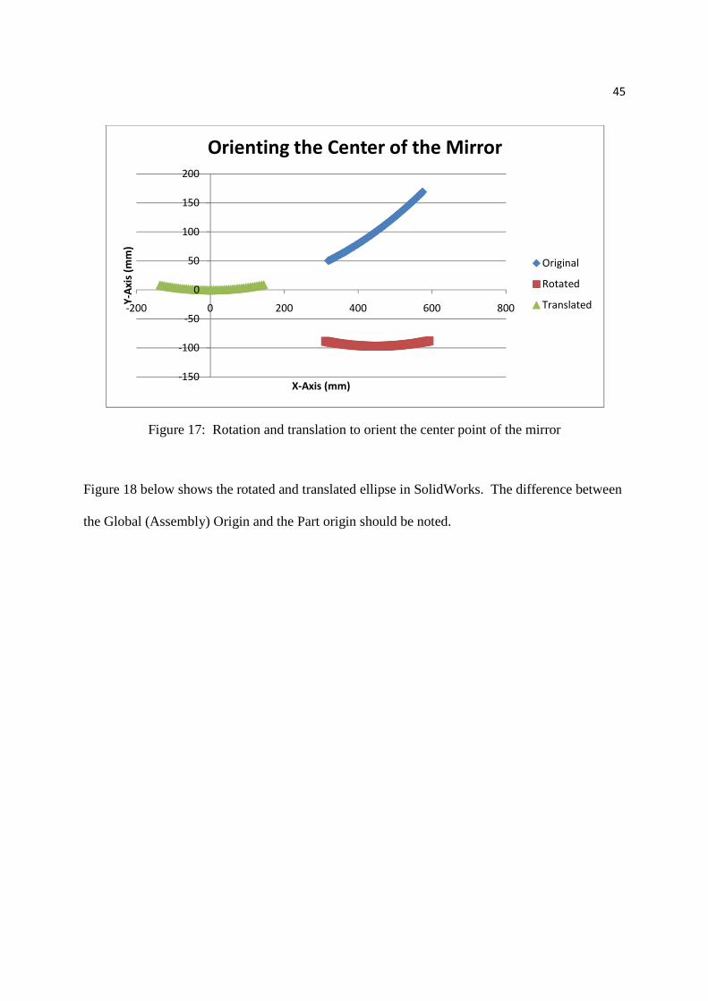
Figure 17: Rotation and translation to orient the center point of the mirror
Figure 18 below shows the rotated and translated ellipse in SolidWorks. The difference between
the Global (Assembly) Origin and the Part origin should be noted.
-150
-100
-50
0
50
100
150
200
-200 0 200 400 600 800
Y-A
xis
(m
m)
X-Axis (mm)
Orienting the Center of the Mirror
Original
Rotated
Translated

46
Figure 18: CAD model of re-oriented ellipse
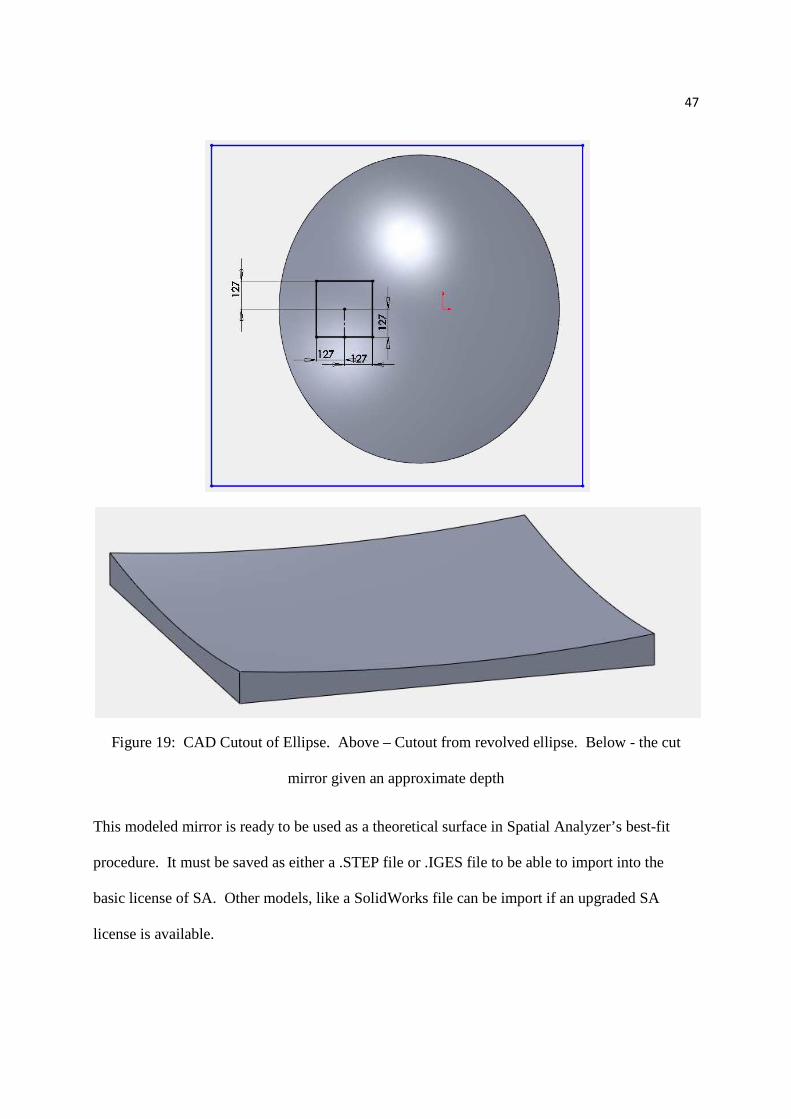
Now the mirror can be cut down to its footprint size. This is done by knowing the side length of
the mirror as well as its optical center. In this case, SuperCam mirror M7 has a side length of
127mm and its optical center is off axis by 447.08mm. With the optical center of the mirror used
as a reference, the mirror is then cut to size. An approximate depth can also be added. This
depth can remain approximate as it is only the optical surface which is of value at this stage in
the procedure. Figure 19 shows the transition from the fully revolved ellipse to the trimmed
down version of the mirror.
47
Figure 19: CAD Cutout of Ellipse. Above – Cutout from revolved ellipse. Below - the cut
mirror given an approximate depth
This modeled mirror is ready to be used as a theoretical surface in Spatial Analyzer’s best-fit
procedure. It must be saved as either a .STEP file or .IGES file to be able to import into the
basic license of SA. Other models, like a SolidWorks file can be import if an upgraded SA
license is available.
48
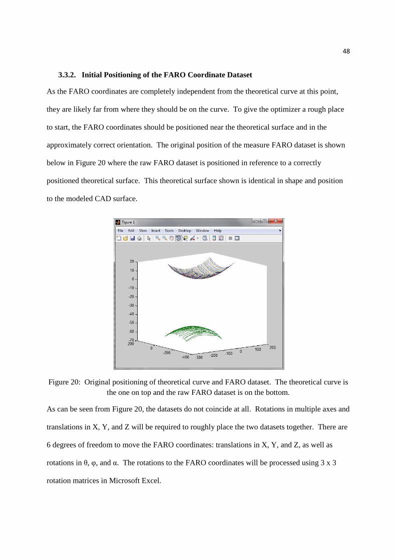
3.3.2. Initial Positioning of the FARO Coordinate Dataset
As the FARO coordinates are completely independent from the theoretical curve at this point,
they are likely far from where they should be on the curve. To give the optimizer a rough place
to start, the FARO coordinates should be positioned near the theoretical surface and in the
approximately correct orientation. The original position of the measure FARO dataset is shown
below in Figure 20 where the raw FARO dataset is positioned in reference to a correctly
positioned theoretical surface. This theoretical surface shown is identical in shape and position
to the modeled CAD surface.
Figure 20: Original positioning of theoretical curve and FARO dataset. The theoretical curve is the one on top and the raw FARO dataset is on the bottom.
As can be seen from Figure 20, the datasets do not coincide at all. Rotations in multiple axes and
translations in X, Y, and Z will be required to roughly place the two datasets together. There are
6 degrees of freedom to move the FARO coordinates: translations in X, Y, and Z, as well as
rotations in θ, φ, and α. The rotations to the FARO coordinates will be processed using 3 x 3
rotation matrices in Microsoft Excel.
49
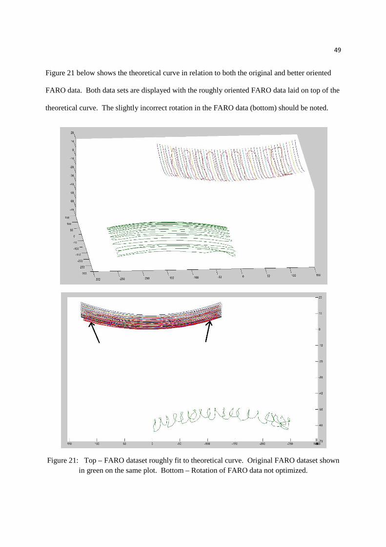
Figure 21 below shows the theoretical curve in relation to both the original and better oriented
FARO data. Both data sets are displayed with the roughly oriented FARO data laid on top of the
theoretical curve. The slightly incorrect rotation in the FARO data (bottom) should be noted.
Figure 21: Top – FARO dataset roughly fit to theoretical curve. Original FARO dataset shown in green on the same plot. Bottom – Rotation of FARO data not optimized.

50
The slight inaccuracy in rotation (shown with black arrows) in this case is not a problem. The
emphasis of this rough placement was to position the FARO dataset nearby the theoretical curve.
The optimization process in future steps will improve upon the placement of the FARO data.
51
3.3.3. Interpolating and Compensating for Probe Offset of FARO Data
With the FARO data roughly positioned, it must now be interpolated and corrected for the probe
offset before it can be used in a best-fit optimization. Both can be accomplished using
MATLAB. The interpolation is done using MATLAB’s Surface Fitting Tool.
The Surface Fitting Tool, called in MATLAB using the command sftool, provides a means of
generating a surface equation and coordinates for a dataset. Once the Surface Fitting Tool is
opened, the X, Y, Z data from the roughly positioned FARO dataset is entered. The type of
surface fit is then selected. Because an easily usable equation is desired, Polynomial is selected
from the surface fit type drop down menu. The order of that polynomial in both the X and Y
directions can be selected. A higher order will improve the accuracy of the surface fit in this
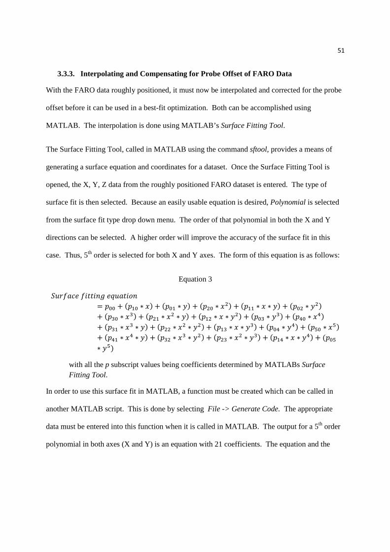
case. Thus, 5th order is selected for both X and Y axes. The form of this equation is as follows:
Equation 3
<=>?@AB ?)CC)DE BF=@C)GD= H�� + (H�� ∗ , + (H�� ∗ �, + (H � ∗ , + (H�� ∗ ∗ �, + (H� ∗ � ,+ (H�� ∗ �, + (H � ∗ ∗ �, + (H� ∗ ∗ � , + (H�� ∗ ��, + (H�� ∗ �,+ (H�� ∗ � ∗ �, + (H ∗ ∗ � , + (H�� ∗ ∗ ��, + (H�� ∗ ��, + (H�� ∗ �,+ (H�� ∗ � ∗ �, + (H� ∗ � ∗ � , + (H � ∗ ∗ ��, + (H�� ∗ ∗ ��, + (H��∗ ��, with all the p subscript values being coefficients determined by MATLABs Surface Fitting Tool.
In order to use this surface fit in MATLAB, a function must be created which can be called in
another MATLAB script. This is done by selecting File -> Generate Code. The appropriate
data must be entered into this function when it is called in MATLAB. The output for a 5th order
polynomial in both axes (X and Y) is an equation with 21 coefficients. The equation and the
52
coefficients are displayed in the MATLAB Command Window when the surface fitting function
is run.
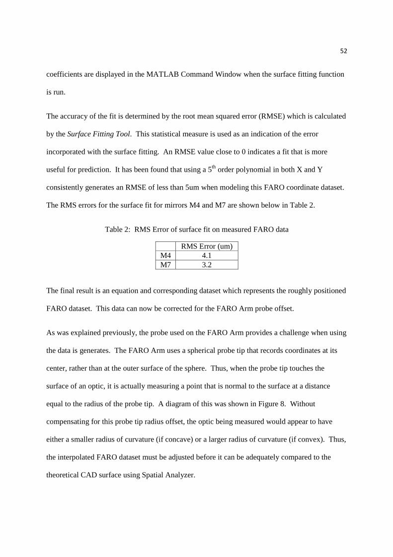
The accuracy of the fit is determined by the root mean squared error (RMSE) which is calculated
by the Surface Fitting Tool. This statistical measure is used as an indication of the error
incorporated with the surface fitting. An RMSE value close to 0 indicates a fit that is more
useful for prediction. It has been found that using a 5th order polynomial in both X and Y
consistently generates an RMSE of less than 5um when modeling this FARO coordinate dataset.
The RMS errors for the surface fit for mirrors M4 and M7 are shown below in Table 2.
Table 2: RMS Error of surface fit on measured FARO data
RMS Error (um) M4 4.1 M7 3.2
The final result is an equation and corresponding dataset which represents the roughly positioned
FARO dataset. This data can now be corrected for the FARO Arm probe offset.
As was explained previously, the probe used on the FARO Arm provides a challenge when using
the data is generates. The FARO Arm uses a spherical probe tip that records coordinates at its
center, rather than at the outer surface of the sphere. Thus, when the probe tip touches the
surface of an optic, it is actually measuring a point that is normal to the surface at a distance
equal to the radius of the probe tip. A diagram of this was shown in Figure 8. Without
compensating for this probe tip radius offset, the optic being measured would appear to have
either a smaller radius of curvature (if concave) or a larger radius of curvature (if convex). Thus,
the interpolated FARO dataset must be adjusted before it can be adequately compared to the
theoretical CAD surface using Spatial Analyzer.
53
To accomplish this, MATLAB will be used to calculate surface normal vectors for the dataset.
These 3 dimensional vectors will then be used to apply the probe radius offset at each individual
point in the direction of the vector. Thus, a new (x,y,z) coordinate will be created for each point.
It should be noted that while Spatial Analyzer has the ability to perform this probe offset
calculation, it will not be sufficient in this application. It has been found that the points that are
corrected for probe offset in SA cannot be used in a best-fit transformation with a theoretical
CAD surface. This seems to be a limitation inherent to Spatial Analyzer.
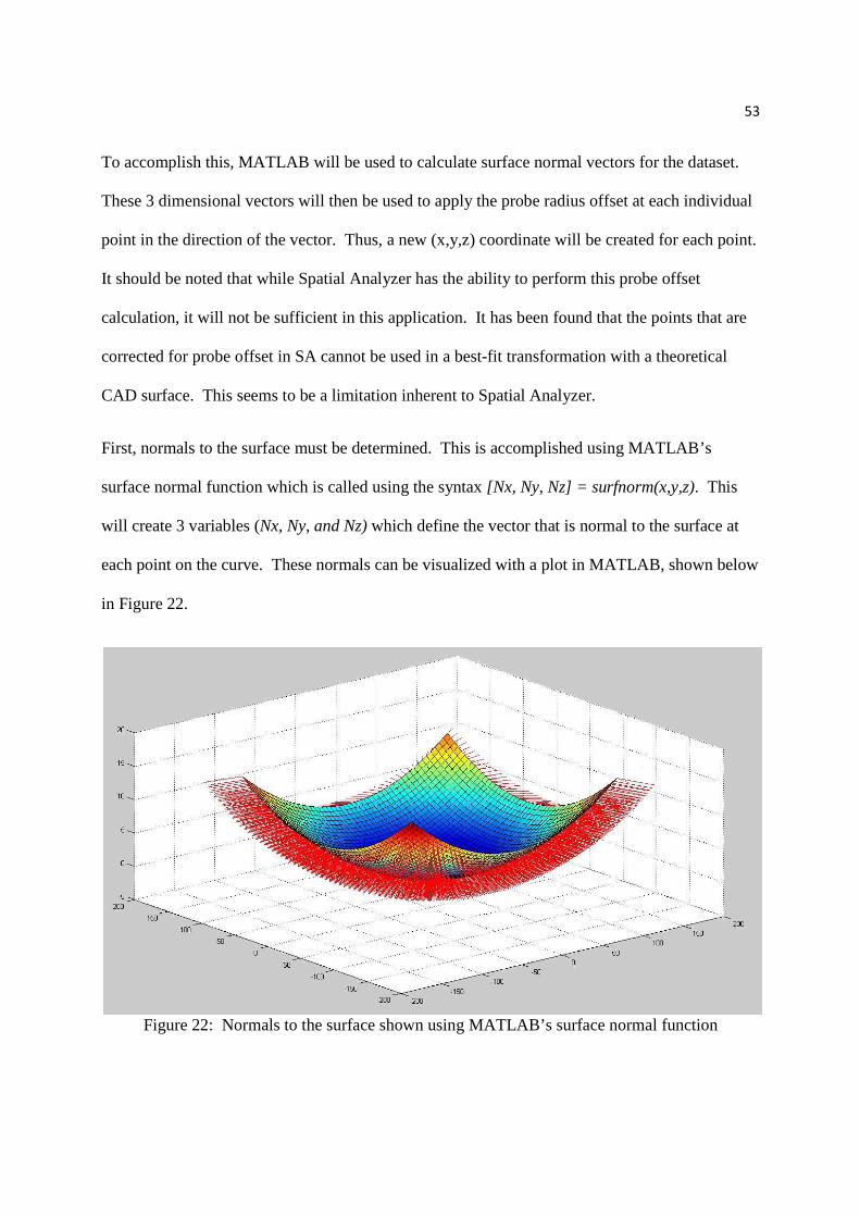
First, normals to the surface must be determined. This is accomplished using MATLAB’s
surface normal function which is called using the syntax [Nx, Ny, Nz] = surfnorm(x,y,z). This
will create 3 variables (Nx, Ny, and Nz) which define the vector that is normal to the surface at
each point on the curve. These normals can be visualized with a plot in MATLAB, shown below
in Figure 22.
Figure 22: Normals to the surface shown using MATLAB’s surface normal function

54
Now that vectors exist for the normal to the surface at each point in this dataset, the probe radius
offset can be compensated for. This is done by multiplying the probe radius, which in this case
was 1.5mm, by the surface normal vectors Nx, Ny, and Nz. The surface vector variables are then
reassigned to include the probe radius offset. This is shown in Equation 4.
I�,�,� = >J7KLM ∗ I�,�,� Equation 4 This determines how much offset must be compensated for in the X, Y, and Z directions. These
offsets are then added to the dataset of the curve. This is done using Equation 5.
(@, N, = (@, N, + I�(@, N, Equation 5 This is repeated for the coordinates of the y and z axes. Finally, because the offset at the center
of the FARO data has a surface normal vertically oriented, that point’s coordinates will have
changed from (0,0,0) to (0,0,-1.5). This -1.5mm can be compensated for by adding 1.5mm in the
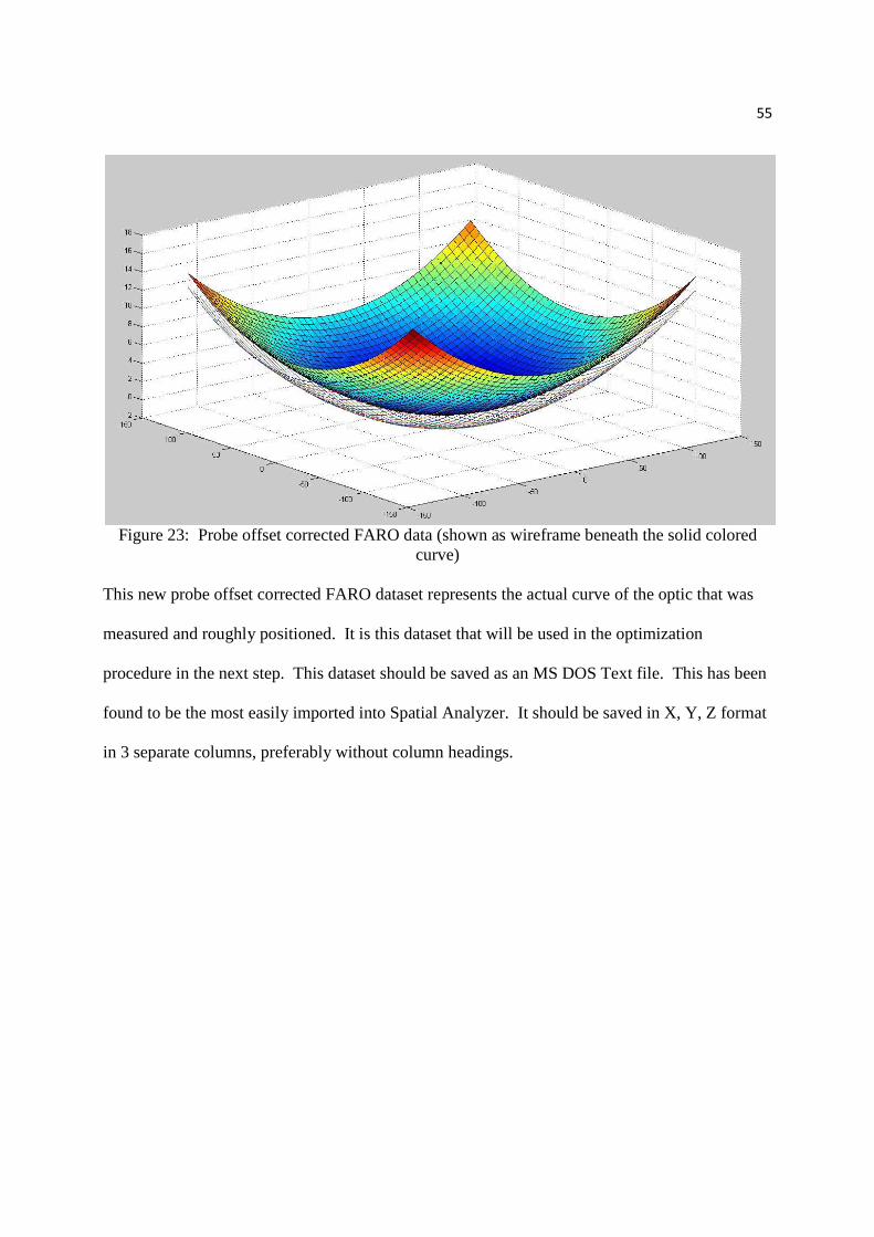
Z direction to the entire dataset. The resulting probe offset corrected dataset is shown below in
Figure 23. The solid colored curve is the same from Figure 22 and the new offset corrected data
is shown below that in wireframe.
55
Figure 23: Probe offset corrected FARO data (shown as wireframe beneath the solid colored
curve) This new probe offset corrected FARO dataset represents the actual curve of the optic that was
measured and roughly positioned. It is this dataset that will be used in the optimization
procedure in the next step. This dataset should be saved as an MS DOS Text file. This has been
found to be the most easily imported into Spatial Analyzer. It should be saved in X, Y, Z format
in 3 separate columns, preferably without column headings.
56
3.3.4. Optimizing the Positioning of the FARO Coordinate Dataset
Now that the FARO coordinate dataset is roughly placed and has been corrected for probe offset,
it is now ready to be best fit to the theoretical surface dataset. There are two methods that can be
used to accomplish this. The easier and more accurate of the two is using Spatial Analyzer. The
second method involves data manipulation as well as the use of the Solver function in EXCEL.
This method is discussed in Appendix A while the method using Spatial Analyzer is explained
here.
In addition to being faster and easier, there are other significant benefits to using Spatial
Analyzer to perform this optimization. As part of this process, the CAD model of the surface of
the mirror will be imported into SA and used as a reference surface. This is preferable to
comparing the discrete FARO dataset to a discrete theoretical dataset, as is done with the
EXCEL optimization method. By providing a theoretical surface as a reference, the FARO
dataset essentially has a continuous dataset to optimize to. An additional benefit to using SA is
that the RMS Error per point is generated when the fit is performed. This provides a figure of
merit for the optimization.
The first step in preparing for SA to optimize the fit between the FARO dataset and reference
CAD surface is to declare the correct units. In this case, microns of error are expected for the fit,
so millimeters are used as the default unit. In Spatial Analyzer, microns are not an available
option. Next, both the CAD surface and FARO dataset are imported. The CAD model is
imported using File -> Import -> Classic CAD Importers. A .STEP file or .IGES file can be
selected here among others. The reference CAD mirror can then be imported. Next, the roughly
fit FARO dataset is imported. The easiest way to do this is to drag the icon of the text file that

57
was generated for this dataset into the main window in SA. An ASCII Import window pops up
like the one shown below in Figure 24.
Figure 24: ASCII Import window which appears when data is imported into SA
As can be seen from Figure 24, a few options must be carefully selected when data is imported.
First, the format of the data is selected based on how the data was stored. If headers were not
used, then the top option X Y Z should be selected. Next, the File Units are selected. In this
case, the data was generated using millimeters so this is selected. The dataset can be given a
Group Name and then it is to be imported. Both the reference CAD surface and the FARO
dataset are now imported into SA and are ready for optimization.
If the same X, Y, Z orientation was used for both the CAD model and the FARO data, then they
should already be roughly fit together upon both being imported into SA. If the coordinate
systems used are different (like if the Y axis in SolidWorks was the Z axis in EXCEL /

58
MATLAB) then Edit -> Move Objects -> Enter Transformation should be used to correctly
rotate either the CAD model or FARO dataset so their axes are comparable.
The alignment can then begin by selecting Analysis -> Best-Fit Transformation -> Points to
Surfaces/Objects -> N-Point Full Fit to Objects. Spatial Analyzer then asks which points to fit.
The FARO dataset should be selected either by holding shift and visually dragging over the
dataset or by pressing F2 and directly choosing the dataset from the Target/Point Selection
window which pops up. Hit enter and the objects to best-fit are then asked for. Again, the CAD
mirror can be manually selected or chosen by pressing F2. Hit enter and when the Target Offset
Values window appears, select the default value of Use the target’s values and press OK. Next,
the pop up window shown below in Figure 25 appears.
Figure 25: Point to Object Best-Fit Transformation pop up window
There are a number of options available in the pop up window shown in Figure 25. The number
of parameters that can be adjusted is, by default 6: translation in X, Y, Z and rotation in θ, α, φ.
The 7th parameter available regards scaling the data. In this case, scaling is not desired. There
are two different optimizations that can be used at this point: the standard optimization, which is

59
selected by choosing Run Optimization or the more involved method which is selected by
choosing Run Direct Search Optimization. It has been found that the standard optimization runs
significantly faster and produces an excellent fit between the FARO data and reference CAD
surface. In either case, once an optimizer is selected, the best-fit transformation begins. A pop
up window called Residuals appears after the optimization is complete. This is shown in Figure
26 below.
Figure 26: Residual pop-up window which appears after a best-fit optimization in SA
The translations and rotations that were used to best-fit the data are shown here as are the
resulting residual error in the fit. As seen in Figure 12, the residual error in the fit is 21.0um.
Finally, the residual error per point is listed. This data will be useful in visually inspecting how
well the optical surface was made so it should be saved using the Save to File button. Next click
Accept and SA asks which objects should be transformed. In this case, it is the FARO dataset
that should be transformed. This will perform the translations and rotations that were found to
be the best fit. Select the FARO dataset and hit enter. Spatial Analyzer then asks which
60
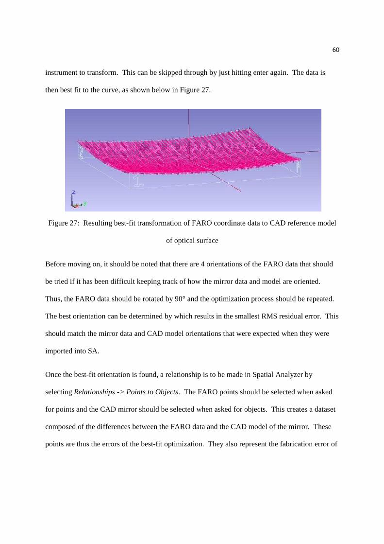
instrument to transform. This can be skipped through by just hitting enter again. The data is
then best fit to the curve, as shown below in Figure 27.
Figure 27: Resulting best-fit transformation of FARO coordinate data to CAD reference model
of optical surface
Before moving on, it should be noted that there are 4 orientations of the FARO data that should
be tried if it has been difficult keeping track of how the mirror data and model are oriented.
Thus, the FARO data should be rotated by 90° and the optimization process should be repeated.
The best orientation can be determined by which results in the smallest RMS residual error. This
should match the mirror data and CAD model orientations that were expected when they were
imported into SA.
Once the best-fit orientation is found, a relationship is to be made in Spatial Analyzer by
selecting Relationships -> Points to Objects. The FARO points should be selected when asked
for points and the CAD mirror should be selected when asked for objects. This creates a dataset
composed of the differences between the FARO data and the CAD model of the mirror. These
points are thus the errors of the best-fit optimization. They also represent the fabrication error of

61
the optic in question. To export this data, a Relationship report can then be created. It is
recommended that the report be exported to an EXCEL file for ease of data handling.
62
3.4. Analyzing the Surface Figure Results
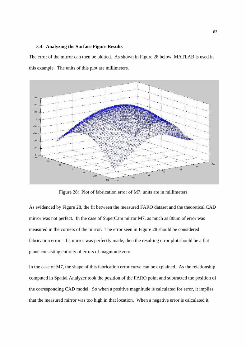
The error of the mirror can then be plotted. As shown in Figure 28 below, MATLAB is used in
this example. The units of this plot are millimeters.
Figure 28: Plot of fabrication error of M7, units are in millimeters
As evidenced by Figure 28, the fit between the measured FARO dataset and the theoretical CAD
mirror was not perfect. In the case of SuperCam mirror M7, as much as 80um of error was
measured in the corners of the mirror. The error seen in Figure 28 should be considered
fabrication error. If a mirror was perfectly made, then the resulting error plot should be a flat
plane consisting entirely of errors of magnitude zero.
In the case of M7, the shape of this fabrication error curve can be explained. As the relationship
computed in Spatial Analyzer took the position of the FARO point and subtracted the position of
the corresponding CAD model. So when a positive magnitude is calculated for error, it implies
that the measured mirror was too high in that location. When a negative error is calculated it
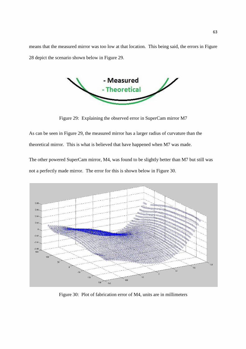
63
means that the measured mirror was too low at that location. This being said, the errors in Figure
28 depict the scenario shown below in Figure 29.
Figure 29: Explaining the observed error in SuperCam mirror M7
As can be seen in Figure 29, the measured mirror has a larger radius of curvature than the
theoretical mirror. This is what is believed that have happened when M7 was made.
The other powered SuperCam mirror, M4, was found to be slightly better than M7 but still was
not a perfectly made mirror. The error for this is shown below in Figure 30.
Figure 30: Plot of fabrication error of M4, units are in millimeters
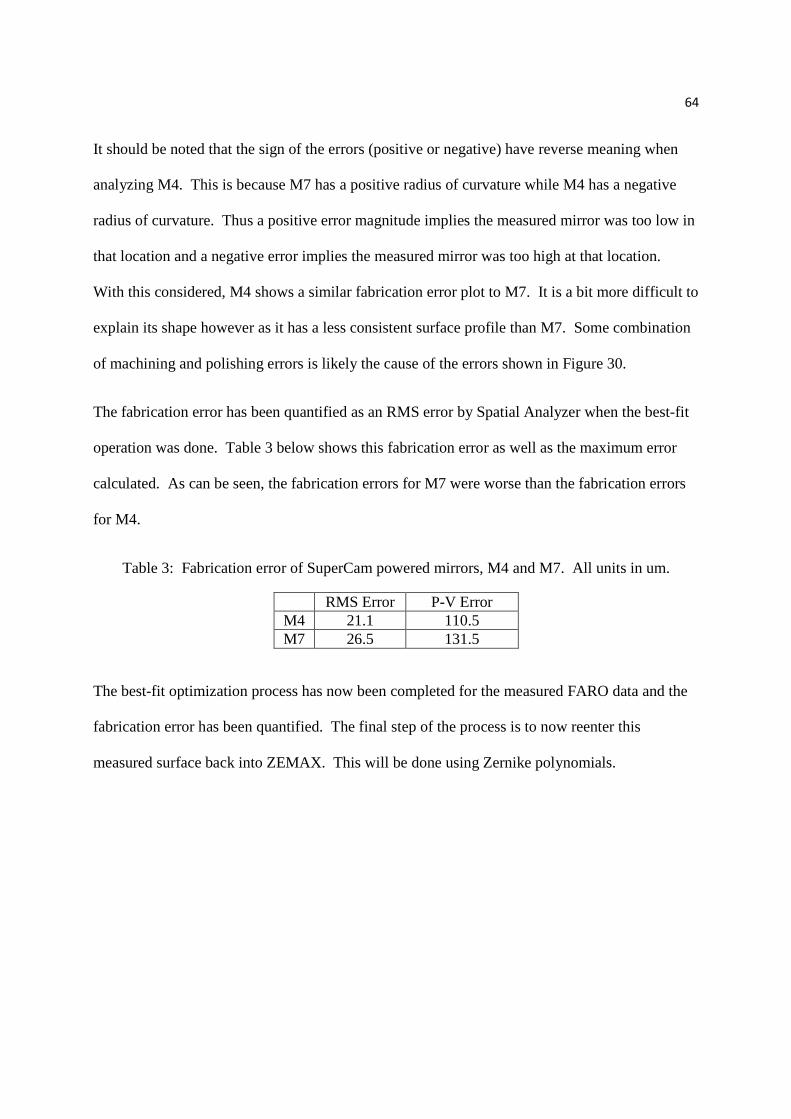
64
It should be noted that the sign of the errors (positive or negative) have reverse meaning when
analyzing M4. This is because M7 has a positive radius of curvature while M4 has a negative
radius of curvature. Thus a positive error magnitude implies the measured mirror was too low in
that location and a negative error implies the measured mirror was too high at that location.
With this considered, M4 shows a similar fabrication error plot to M7. It is a bit more difficult to
explain its shape however as it has a less consistent surface profile than M7. Some combination
of machining and polishing errors is likely the cause of the errors shown in Figure 30.
The fabrication error has been quantified as an RMS error by Spatial Analyzer when the best-fit
operation was done. Table 3 below shows this fabrication error as well as the maximum error
calculated. As can be seen, the fabrication errors for M7 were worse than the fabrication errors
for M4.
Table 3: Fabrication error of SuperCam powered mirrors, M4 and M7. All units in um.
RMS Error P-V Error M4 21.1 110.5 M7 26.5 131.5
The best-fit optimization process has now been completed for the measured FARO data and the
fabrication error has been quantified. The final step of the process is to now reenter this
measured surface back into ZEMAX. This will be done using Zernike polynomials.

65
3.5. Determining Effect on Optical Performance of THz System 3.5.1. Why Use Zernike polynomials?
Zernike polynomials are a sequence of polynomials that are useful in expressing wavefront data.
The reason is because the polynomials are of the same form as the types of aberrations often
observed in optical tests. The first 10 Zernike functions are shown below with their coinciding
aberrations.
Figure 31: First 10 Zernike functions with equations and aberrations (Fricker)
Though using Zernike polynomials to determine what aberrations are present in a wavefront is
quite useful, it is not the main reason they were used in this case. The main reason is simply that
they provided a convenient means of inputting an irregular surface into ZEMAX. It was found
that the surface that was machined and polished into SuperCam mirrors M4 and M7 could not be
well defined using only standard conic equation parameters (conic constant (k), radius of
curvature (c)). Inversely, the use of Zernike polynomials was found to model M4 and M7’s

66
irregular surface with good accuracy while providing an easy way of entering the surface into
ZEMAX.
Zernike polynomials are most frequently used to describe wavefront error associated with an
optical surface. In this case, Zernike polynomials will be used to describe the fabrication error of
an optical surface. This is a convenient way to input an irregular surface into ZEMAX. The
original ZEMAX conic parameters of the optical surface will remain while the irregularities of
the measured surface will be added on top of it. The procedure to do this will be discussed in
greater detail later.

67
3.5.2. How to Generate Zernike Polynomial Coefficients
In order to generate Zernike polynomial coefficients, an open source MATLAB script is used.
The script is called deco.m and can be downloaded for free here:
http://www.mathworks.com/matlabcentral/fileexchange/17950
In addition to deco.m, two open source MATLAB functions are also needed: zernfun and
zernfun2. These can be downloaded for free here:
http://www.mathworks.com/matlabcentral/fileexchange/7687
Once both functions have been downloaded and imported into MATLAB, a set of X, Y, Z data
can be input into the deco.m script. This data should be the probe SA dataset representing the
difference between the measured and theoretical mirror surfaces. In order to enter this dataset
into deco.m, the X and Y data must be normalized to a circle with a radius of 1. The
normalization of the X and Y data can be accomplished in either EXCEL or MATLAB. Making
the dataset circular rather than and n x m matrix is most easily done in MATLAB. To do this, an
equation is generated using the Surface Fitting Tool. Next, the data must be trimmed to a circle.
Though the mirrors are all rectangular in shape, they must be modeled as a circle in order to be
decomposed into Zernike polynomials. Thus, this modeling does not take into account the
fabrication errors at the corners of each mirror. This is not ideal but it is the best that can be
done to reenter the mirror into ZEMAX. In order to trim the dataset to a circle, a set of
cylindrical coordinates (θ,r) are created and are converted into Cartesian coordinates. This is
done using the MATLAB function [x,y] = pol2cart(theta,r). These [x,y] coordinates can then be
entered into the new surface fitting equation to generate a normalized, circular dataset. Figure 32
below shows the same curve from Figure 28 above but is now normalized and with a circular
footprint.

68
Figure 32: Normalized and circular FARO dataset of fabrication errors ready for Zernike
decomposition
The one variable of significant note within the deco.m script is p, which indexes the number of
Zernike modes to be used in the decomposition. This variable can be adjusted depending on how
well the Zernike polynomials are representing the dataset. The metric for determining the
quality of fit is the Residuals plot which is output by deco.m. The Residuals plot shows where
on the circle the Zernike decomposition was unable to account for the surface or wavefront. The
smaller the magnitude of the residuals plot, the more accurately the Zernike decomposition
represents the surface. As the Zernike terms are orthogonal, or statistically independent of one
another, often the greater number of terms used, the more accurate the surface fit will become.

69
As is shown below in Table 4, it was found that there was a limit to an improvement in residual
error based on the number of Zernike terms used.
Table 4: Maximum residual error in relation to number of Zernike terms used to model fabrication error
Zernike Terms Maximum Residual Error [um]
9 12
13 4.5
17 4.2
21 .07
25 .14
29 .15
The increase in residual error after 21 terms is possibly a result of higher frequency terms being
used to represent local errors while inadvertently introducing residual errors on the rest of the
mirror. Because the residual errors were found to more than adequately model the fabrication
errors of the SuperCam mirrors, no further analysis of this phenomenon were pursued.
As can be seen from Table 4, the number of Zernike terms that is best in the case of SuperCam
mirror M7 is when p = 20 (21 total terms).
The output of the deco.m script is a list of Zernike polynomial coefficients. The number of
coefficients depends on the number of Zernike terms selected with the variable p. These
coefficients are now ready for the last step before they can be input back into ZEMAX.
3.5.3. Making Zernike Coefficients Compatible with ZEMAX

70
In order to prepare the Zernike coefficients for being entered into ZEMAX, they must be
normalized and ordered to match a format that ZEMAX will accept. The format that was used is
the Zernike Standard set of polynomials. This list of polynomials has a required order in which
the Zernike terms must be entered. It was found early on that while the MATLAB Zernike script
output a list of coefficients that was close to the order required of the Zernike Standard list, it
was not the same. A short list of the required order of Zernike Standard terms and the Zernike
MATLAB script terms is shown below in Table 5. A complete list of Zernikes is displayed in
Appendix A.
Table 5: Comparison of first 10 Zernike modes (ZEMAX User’s Manual 201-202) (Fricker)
Zernike Standard MATLAB Term Z(ρ,θ) Z(ρ,θ)
1 1 1 2 √4QAGR� QAGR� 3 √4QR)D� QR)D� 4 √3(2Q − 1, Q AGR2� 5 √6(Q R)D2�, 2Q − 1 6 √6(Q AGR2�, Q R)D2� 7 √8(3Q� − 2Q,R)D� Q�AGR3� 8 √8(3Q� − 2Q,AGR� (3Q� − 2Q,AGR� 9 √8Q�R)D3� (3Q� − 2Q,R)D� 10 √8Q�AGR3� Q�R)D3�
As can be seen from Table 5, not only is the order of the Zernike terms different between sets,
but there are coefficients on the Zernike Standard set that the MATLAB set does not have. This
trend continues for the larger Zernike terms. As the Zernike Standard terms are to be entered
into ZEMAX, the MATLAB coefficients must use the same normalization factors and must be
reordered. The normalization factors will be addressed first.

71
The benefit of using a preexisting MATLAB script is that much of the code writing is already
complete. The challenge is that preexisting scripts can be poorly documented. This was the case
for this particular script. The result is that some reverse engineering was necessary to determine
exactly what the script was doing. Specifically, some testing needed to be done to determine if
the output Zernike coefficients were taking into account normalization factors before they were
output, or if this needed to be done afterwards. Thus, a test was devised to answer this question.
As any equation could be entered into deco.m, the exact equations that are shown in Table 5
were entered to see what the resulting Zernike coefficient would be. If the output coefficient was
1, then it would be known that the normalization factors were being utilized before the
coefficient was output. Any answer but 1 would indicate the opposite.
The results from this test are shown below in Table 6. The Zernike coefficients that were output
by MATLAB for each individual equation are in the Coefficient column.

72
Table 6: Normalization factors for MATLAB Zernike decomposition
# m n Equation Coefficient Inverse
Coefficient
Standard Zernike
Normalization Coefficients
1 0 0 1 1.772 0.564 0.564 2 1 1 QAGR� 0.886 1.128 0.564 3 1 -1 QR)D� 0.886 1.128 0.564 4 2 -2 Q AGR2� 0.723 1.381 0.563 5 2 0 2Q − 1 1.023 0.976 0.564 6 2 2 Q R)D2� 0.723 1.381 0.564 7 3 -3 Q�AGR3� 0.627 1.594 0.563 8 3 -1 (3Q� − 2Q,AGR� 0.627 1.594 0.563 9 3 1 (3Q� − 2Q,R)D� 0.627 1.594 0.564 10 3 3 Q�R)D3� 0.626 1.595 0.563 11 4 -4 Q�AGR4� 0.564 1.770 0.562 12 4 -2 (4Q� − 3Q ,AGR2� 0.561 1.780 0.563 13 4 0 6Q� − 6Q + 1 0.794 1.258 0.563 14 4 2 (4Q� − 3Q ,R)D2� 0.561 1.780 0.559 15 4 4 >�R)D4� 0.557 1.795 0.567 16 5 -5 Q�AGR5� 0.512 1.952 0.562 17 5 -3 (5Q� − 4Q�,AGR3� 0.513 1.948 0.562 18 5 -1 (10Q� − 12Q� + 3Q,AGR� 0.513 1.946 0.562 19 5 1 (10Q� − 12Q� + 3Q,R)D� 0.513 1.946 0.562 20 5 3 (5Q� − 4Q�,R)D3� 0.513 1.949 0.563 21 5 5 Q�R)D5� 0.512 1.952 0.563 22 6 -6 QUAGR6� 0.474 2.107 0.560 23 6 -4 (6QU − 5Q�,AGR4� 0.479 2.084 0.561 24 6 -2 (15QU − 20Q� + 6Q ,AGR2� 0.476 2.099 0.561 25 6 0 20QU − 30Q� + 12Q − 1 0.673 1.484 0.566 26 6 2 (15QU − 20Q� + 6Q ,R)D2� 0.476 2.099 0.557 27 6 4 (6QU − 5Q�,R)D4� 0.471 2.120 0.563 28 6 6 QUR)D6� 0.474 2.107 0.563
As can be seen in Table 6, the Zernike coefficients that were output by MATLAB when the
Zernike equations were entered individually are not equal to 1. This verifies that any
normalization factors that are necessary are not included in the Zernike calculations before
coefficients are output. Thus, this must be done after MATLAB outputs coefficients. The 6th
column in Table 6, titled Inverse Coefficient, is the normalization factor that needs to be used.
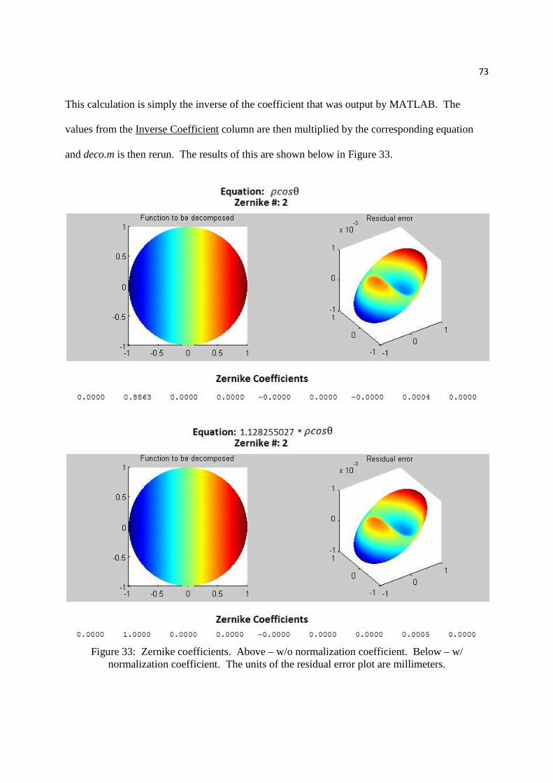
73
This calculation is simply the inverse of the coefficient that was output by MATLAB. The
values from the Inverse Coefficient column are then multiplied by the corresponding equation
and deco.m is then rerun. The results of this are shown below in Figure 33.
Figure 33: Zernike coefficients. Above – w/o normalization coefficient. Below – w/
normalization coefficient. The units of the residual error plot are millimeters.

74
As can be seen from Figure 33, the Zernike coefficient changes from 0.8863 to 1.0000 when the
inverse of the original coefficient is multiplied by its corresponding equation. It is also worth
noting that because this was the 2nd equation on the MATLAB Zernike mode set, the coefficient
that is output is in the 2nd spot. This helps to verify that the order of the Zernike equations in the
MATLAB script is well understood. It was also found that the residual errors from each Zernike
mode are very small. In the case of Zernike mode 2, shown in Figure 33, the maximum residual
error was less than 1um. This shows that the Zernike script is doing an excellent job of
representing the input equation with Zernike polynomials.
The next step of the process is to reorder the modified MATLAB Zernike coefficients. The goal
is to make the order of Zernikes match the Zernike Standard Coefficients so that they can be
entered into ZEMAX. This is done in EXCEL using a template like the one shown in Table 7.
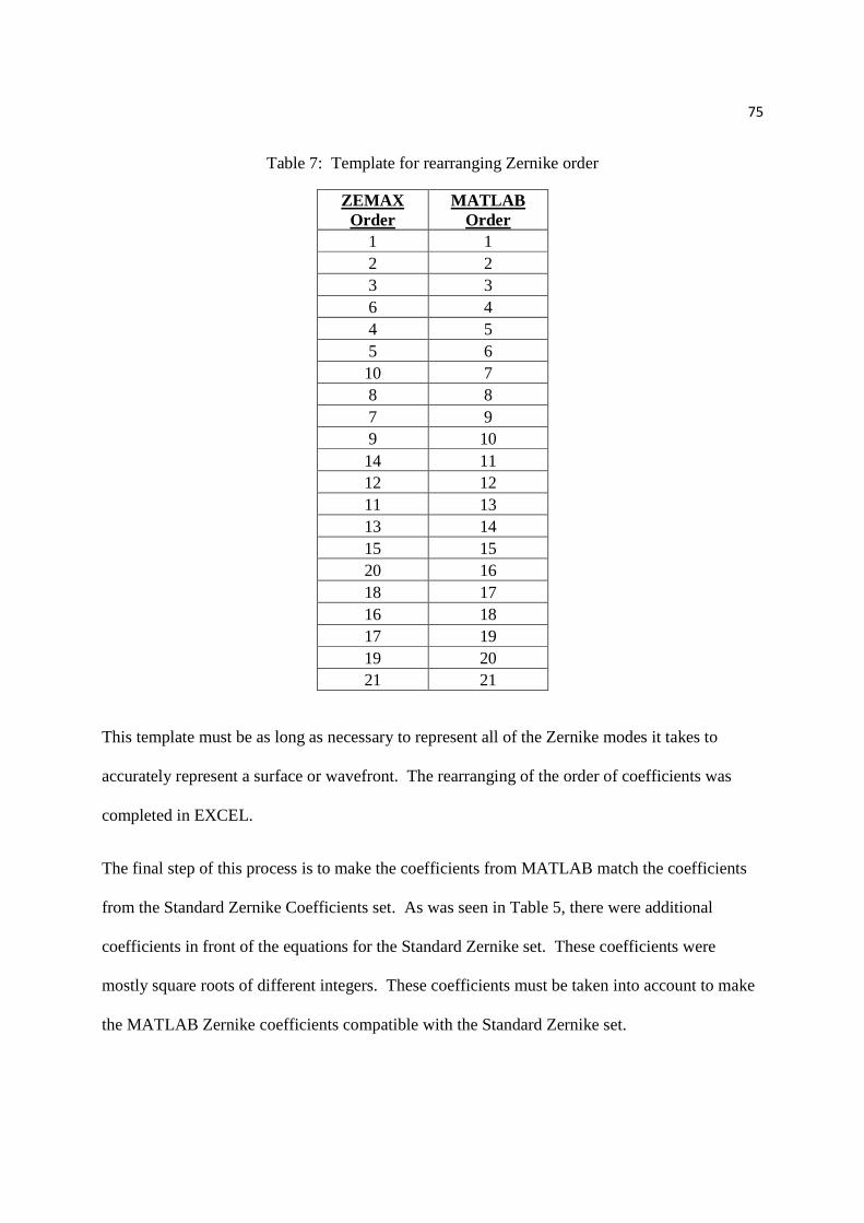
75
Table 7: Template for rearranging Zernike order
ZEMAX Order
MATLAB Order
1 1 2 2 3 3 6 4 4 5 5 6 10 7 8 8 7 9 9 10 14 11 12 12 11 13 13 14 15 15 20 16 18 17 16 18 17 19 19 20 21 21
This template must be as long as necessary to represent all of the Zernike modes it takes to
accurately represent a surface or wavefront. The rearranging of the order of coefficients was
completed in EXCEL.
The final step of this process is to make the coefficients from MATLAB match the coefficients
from the Standard Zernike Coefficients set. As was seen in Table 5, there were additional
coefficients in front of the equations for the Standard Zernike set. These coefficients were
mostly square roots of different integers. These coefficients must be taken into account to make
the MATLAB Zernike coefficients compatible with the Standard Zernike set.

76
This is done by dividing the normalized and reordered Zernike coefficients by the coefficient
(square root term) of each individual Standard Zernike term. An example is shown below using
the 2nd Zernike term which was used in Figure 33. As shown in Table 5, the square root term for
the 2nd Zernike is √4. The value 1.128255027 is the inverse of the Zernike coefficient that was
output when the equation for the 2nd Zernike term was entered into deco.m.
1√4 ∗ 1.128 = 0.564
This value of 0.564 is the final coefficient needed for converting the Zernike coefficients from
MATLAB into coefficients that are ready for inputting into ZEMAX. The full table of these
coefficients is shown in the last column of Table 6 above.

77
3.5.4. Generating Zernike Coefficients for Optimized FARO Dataset
Finally, the best fit FARO dataset that was optimized is ready to be decomposed into Zernike
coefficients. First, an equation must be created using MATLABs Surface Fitting Tool. This is
because deco.m requires Z values that are in an [m x n] matrix and the optimized FARO data is
in three columns. Generating a new surface for this optimized data is quite easy and the error
introduced into the process is negligible.
Once a dataset for the optimized FARO data surface has been generated, it can be input into
deco.m. Some experimenting should be performed to determine the number of Zernike modes
that are calculated. The number of modes that return the smallest residual error should be used.
A set of Zernike coefficients is then returned from deco.m which describes the measured surface
of the optic.
These coefficients are then reordered based on the template shown in Table 7. Finally, they are
multiplied by the Standard Zernike Normalization Coefficients that were calculated. These are
shown in the final column of Table 6. The resulting Zernike coefficients are now ready to be
entered into ZEMAX.

78
3.5.5. Entering Zernike Coefficients into ZEMAX
A great deal of work has been done to this point to produce a set of Zernike coefficients that can
be input into ZEMAX. Fortunately this past work makes the work in ZEMAX very simple.
First, the original ZEMAX file of the optical assembly should be opened and the most useful
metrics for quantifying optical performance should be recorded. This includes a 3D layout of the
optical assembly, an OPD Fan at the focal plane, and a Foot Print diagram at the focal plane.
These will be compared with the measured optical surfaces once they are entered.
In the case of the SuperCam relay optics, there are only two powered optical surfaces which
needed to be measured. Thus only two surfaces in the original ZEMAX file need to be modified
to include Zernike terms. This is done by changing the Surface Type of the powered surface
from Standard to Zernike Standard Sag. This will add two Zernike decenter columns for that
surface in the Lens Data Editor. These values indicate how far off-axis the Zernike terms that
will be entered are to be located. The values for the Aperture Decenter of the mirror should be
entered here. This will align the Zernike terms with the optical surface in question.
Next the Extra Data Editor window is opened and the surfaces which will have Zernike terms
entered are identified. These surfaces will have a number of useful columns in which to enter
data. This is shown below in Figure 34.
Figure 34: ZEMAX window Extra Data Editor which is used to enter Zernike coefficients
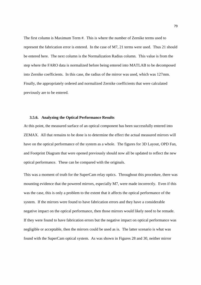
79
The first column is Maximum Term #. This is where the number of Zernike terms used to
represent the fabrication error is entered. In the case of M7, 21 terms were used. Thus 21 should
be entered here. The next column is the Normalization Radius column. This value is from the
step where the FARO data is normalized before being entered into MATLAB to be decomposed
into Zernike coefficients. In this case, the radius of the mirror was used, which was 127mm.
Finally, the appropriately ordered and normalized Zernike coefficients that were calculated
previously are to be entered.
3.5.6. Analyzing the Optical Performance Results
At this point, the measured surface of an optical component has been successfully entered into
ZEMAX. All that remains to be done is to determine the effect the actual measured mirrors will
have on the optical performance of the system as a whole. The figures for 3D Layout, OPD Fan,
and Footprint Diagram that were opened previously should now all be updated to reflect the new
optical performance. These can be compared with the originals.
This was a moment of truth for the SuperCam relay optics. Throughout this procedure, there was
mounting evidence that the powered mirrors, especially M7, were made incorrectly. Even if this
was the case, this is only a problem to the extent that it affects the optical performance of the
system. If the mirrors were found to have fabrication errors and they have a considerable
negative impact on the optical performance, then those mirrors would likely need to be remade.
If they were found to have fabrication errors but the negative impact on optical performance was
negligible or acceptable, then the mirrors could be used as is. The latter scenario is what was
found with the SuperCam optical system. As was shown in Figures 28 and 30, neither mirror
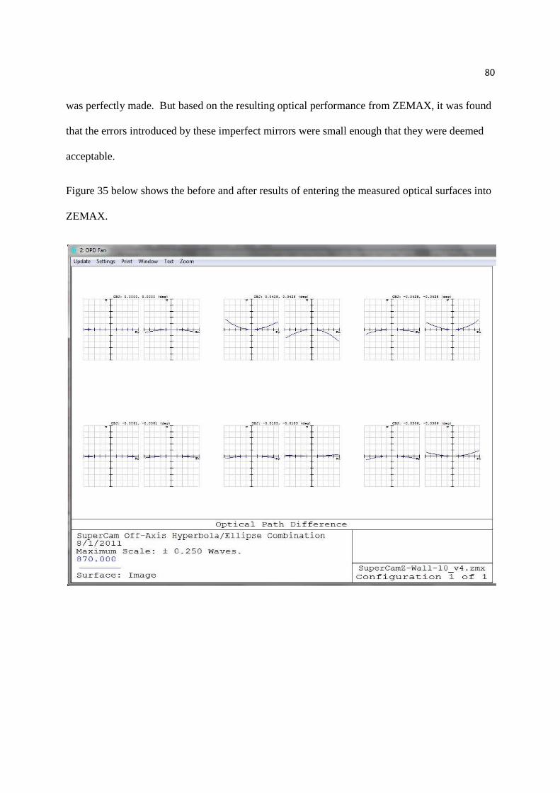
80
was perfectly made. But based on the resulting optical performance from ZEMAX, it was found
that the errors introduced by these imperfect mirrors were small enough that they were deemed
acceptable.
Figure 35 below shows the before and after results of entering the measured optical surfaces into
ZEMAX.

81
Figure 35: OPD Fan of the optical performance of SuperCam. Above – before Zernike terms were included into powered optical surfaces. Below – after Zernike terms were included into
powered optical surfaces.
The OPD Fan is a useful way to observe how the optical performance of the system has changed.
The OPD Fans shown above in Figure 35 depict the wavefront error in pupil coordinates at the
focal plane of the optical system. The various plots shown represent the different field angles of
light that have passed through the optical system. It should be noted that in the scale for both of
these plots is ��, which is considered the threshold of acceptable optical performance. Though the
OPD Fan for each field angle depicts wavefront error that seems to near this �� threshold, these
values are P-V errors, not RMS, which provide a better representation of typical optical

82
performance. This being said, the RMS wavefront error for before and after inserting the as-built
mirrors are shown below in Table 8.
Table 8: RMS Wavefront error of optical system before and after as-built mirrors are entered
RMS Wavefront Error [um] Before As-Built Mirrors Entered V34
After As-Built Mirrors Entered V32.25
Thus, the resulting optical performance is quite encouraging. It was found that while some new
errors were introduced at the focal plane, they remained very acceptable as they are well below
the �� acceptable RMS wavefront error. It should be noted that the wavefront error introduced
into the system by imperfect mirrors is only one piece of the total error puzzle. The following
analysis has assumed that the alignment of this as-built optical system is perfect, which it
certainly will not be in reality.
An updated tolerance analysis must thus be completed using the as-built optical system. As the
additional wavefront error resulting from surface error was quite small, the alignment tolerances
were not affected much. The same alignment tolerances discussed in Chapter 1 still hold true
while the overall RMS wavefront error of the system increases to ���.W�. This is still well within
the acceptable total RMS wavefront error for the system.

83
3.6. Considering Procedural Errors
The final product of this surface figure analysis is a determination of the overall optical
performance of the SuperCam relay optics after measured surfaces have been entered. The
accuracy of this procedure is limited by a combination of errors. These errors during the
following processes:
• Measurement accuracy of FARO Arm when measuring surface of optics
• Construction of mirror surface using a spline in SolidWorks
• Surface fitting procedure using MATLAB’s Surface Fitting Tool
• Best fitting measured dataset to theoretical CAD surface in Spatial Analyzer
• Zernike decomposition of mirror fabrication errors
The measurement accuracy of the FARO Arm, which is 28um, is an immediate source of error in
this procedure, as measuring the optical surface is the first step. This is an error that every
measured point is subjected to and should be considered non-negligible. Next, the process of
generating the optical surface with a spline in SolidWorks provides a maximum error of 0.01um.
This is considered negligible. The surface fitting procedure used in MATLAB provides an RMS
error of less than 5um. The next source of error in this procedure is during the best-fit
optimization of the measured FARO data to the theoretical CAD surface. The procedural error
associated with this transformation is difficult to quantify. This process resulted in and RMS
error of 20-25um but this was considered fabrication error of the optical surface, not procedural
error. There is no doubt that this optimization introduced some error that was not fabrication
error though it is all bundled into one error value. However, it is fair to assume that the error in
the optimization itself is less than the 20-25um RMS of fabrication error that was calculated.

84
Finally, the MATLAB Zernike decomposition process provided a maximum of .07um of error.
In all practicality, this is considered negligible.
Considering all of these lossy processes, there is value in making a reasonable estimate of the
combined procedural errors. This is done by taking the square root of the sum of the squares of
each error in this procedure. This is done because each error can be considered independent of
the other errors and is thus should not simply be added together. This being said, a reasonable
estimate for the procedural errors in this system is shown below.
!28 +. 01 + 5 + 25 +. 07 = 37.9=� Z[<
This means that the procedural errors provide an additional RMS error of less than 40um, which
results in an additional wavefront error of � .�. Even considering this additional procedural error,
the total error in the system should be considered small enough to have confidence in this
procedure.

85
4. Chapter 3: Aligning THz Optics
4.1. Introduction
The FARO Arm is a coordinate measuring instrument with a wide range of applications. It is
capable of providing coordinate data for determining the surface curvature of a THz optic. This
second application for the FARO Arm continues to expand its usefulness. Our goal was to use
the FARO Arm to align optical components in a larger optical assembly. Again, the SuperCam
optical system is used as an example. This provides a significant challenge as SuperCam has a 7
mirror array with the 2 off-axis powered mirrors that were previously analyzed.
As with the previous procedure in determining the surface curvature of an optic, accomplishing
this will require a multi step procedure. The first step of the process is to create a mechanical
reference for the optical surface. This is done by machining fiducials into the sides of the optical
components. These fiducials and the optical surface will then be measured with the FARO Arm
at the same time. Next, these coordinates will be compared to the theoretical curve of each optic
and their position will be optimized to best fit to that curve. This is the same procedure that was
used in Chapter 2 where the surface figure of an optic was determined. This being said, some
rotations and translations of datasets can be reused from the previous analysis. Next, the
fiducials will be modeled into the mirror using SolidWorks. These fiducial positions are based
on the coordinates collected by the FARO Arm. Once each optical component has been
modeled, it will then be placed back into the SolidWorks assembly. At this point, the real
mirrors should be in roughly their correct mounted positions within their mounting structure.
Then the FARO Arm is to be mounted in a position near the mirror mounting structure so that
each optical component in the array can be reached with the probe. Using the FARO Arm and
Spatial Analyzer (SA), coordinates will be taken for three fiducials per mirror. These

86
coordinates will then be compared to the corresponding position in the mirror array model that
has been imported into SA. Based on how the real coordinates of each fiducial relates to the
modeled coordinates, the mirrors will be repositioned accordingly.

87
4.2. Creating Reference Fiducials / Mechanical Reference for Optical Surface
The need to generate a set of mechanical references for each optical element is the result of how
an optical system is designed and how the FARO Arm records each coordinate. In optical
system design, it is the optical surfaces which are used as references to designate correct spacing
and positioning. For this very reason it is the optical surfaces of each component which must be
used as reference surfaces for alignment.
With this in mind, the measurement technique of the optical surface must be examined. In this
case this is done using the FARO Arm. As shown in Figure 8, the FARO Arm probe records
coordinates at the center of a spherical probe tip, rather than at the surface where it touches the
optic. Thus, when a curved surface is measured, the coordinate that is recorded is displaced by
the radius of the probe tip in a direction normal to the optical surface. At the same time,
recording measurements of one surface makes it difficult to fully constrain that surface. In the
case of flat surfaces, data is only taken in 2 planes: no data taken out of plane is recorded. To
fully constrain a point in space, all 3 planes must be fully constrained. This hypothetically can
be less of a problem with curved surfaces as data is taken out of plane. The challenge in this
case is twofold. First off, a curved surface must be machined to very tight tolerances to use it as
a reference surface. In the case of the SuperCam mirrors, it was found that the optical surface
could not be used as a reference because surface figure error had been introduced in the
fabrication process. The second challenge with both curved and flat surfaces is that it is difficult
to constrain the position of the probe. There are no mechanical stops to constrain where the
probe is when a reference coordinate is taken. Thus, it is difficult to know if this coordinate was
taken at the correct position. This is a problem if this coordinate is supposed to be used as a
reference.
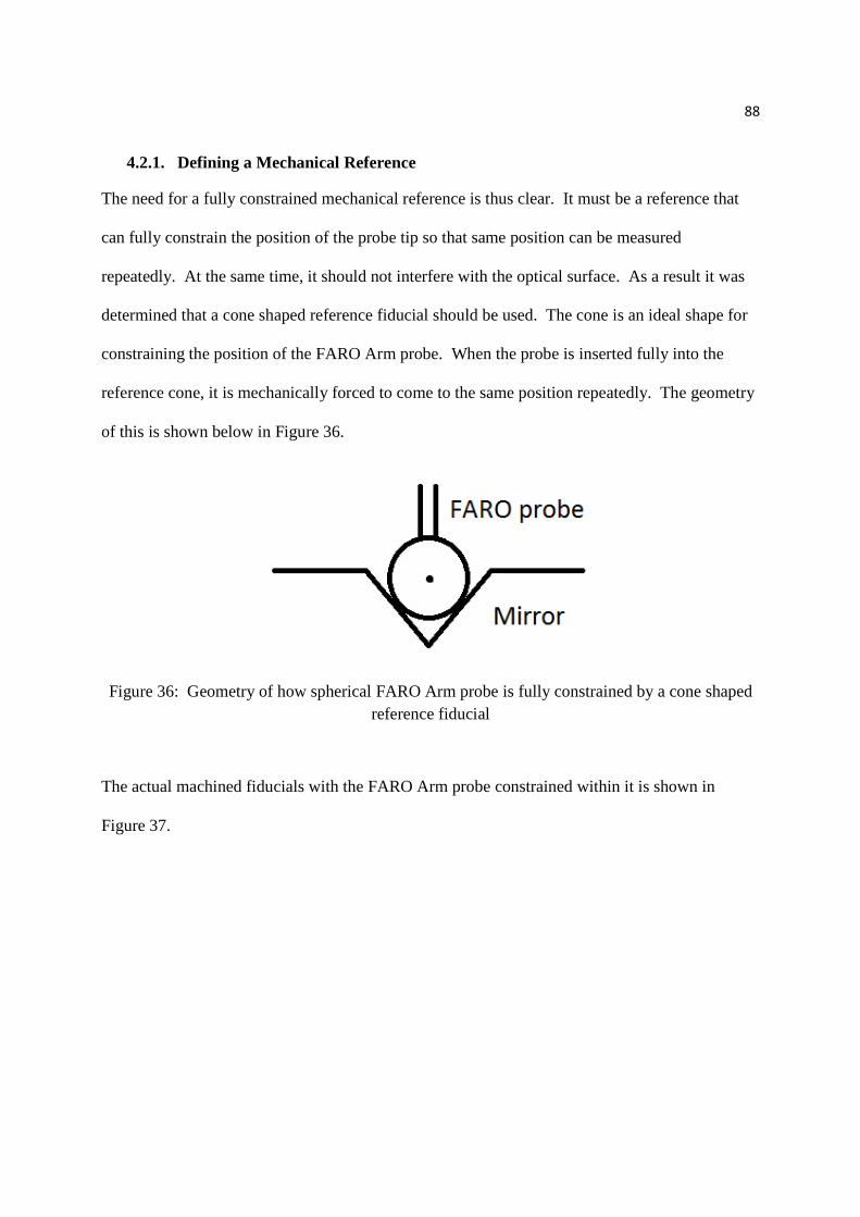
88
4.2.1. Defining a Mechanical Reference
The need for a fully constrained mechanical reference is thus clear. It must be a reference that
can fully constrain the position of the probe tip so that same position can be measured
repeatedly. At the same time, it should not interfere with the optical surface. As a result it was
determined that a cone shaped reference fiducial should be used. The cone is an ideal shape for
constraining the position of the FARO Arm probe. When the probe is inserted fully into the
reference cone, it is mechanically forced to come to the same position repeatedly. The geometry
of this is shown below in Figure 36.
Figure 36: Geometry of how spherical FARO Arm probe is fully constrained by a cone shaped reference fiducial
The actual machined fiducials with the FARO Arm probe constrained within it is shown in
Figure 37.

89
Figure 37: Machined fiducial with FARO Arm probe constrained within it
In the case of a mirror with depth, such as with SuperCam, it was found that an ideal position for
these reference fiducials is on each of the four sides of the mirror. This is a practical position
because the fiducials are accessible: when the mirror is being aligned using the FARO Arm, they
can be easily reached. In order to improve accessibility, it was decided that between 3 and 5
fiducials would be machined into each side of each mirror. This would ensure that a fiducial will
be accessible when the alignment is being performed. Having fiducials machined into the side of
a mirror also prevents interference with the optical surface. Depending on the construction and
material of a mirror or lens, machining fiducials into the mirror itself might be a poor decision.
Consideration should be given into whether the machining stresses will change the surface
curvature of the mirror. In cases of very thin optical components or optics made from brittle

90
materials, an alternative method of creating fiducials, such as gluing them on, would likely be a
better decision.
This particular geometry, with fiducials being positioned on the sides of a mirror, makes the
FARO Arm an ideal choice for a CMM. Many CMMs only have the ability to take a set of
coordinates from one direction. In this case, only the top surface of an optic could be measured
at a given time. But with the FARO Arm, the optical surface as well as the machined fiducials
can be measured in the same dataset. This is a significant advantage of using the FARO Arm
for this application.
The cone shaped fiducials can now be machined into the sides of each mirror. This is a
surprisingly simple process as the depth of each fiducial does not need to be held constant. Thus,
these fiducials can be created using a large drill bit and a hand drill. Similarly, the spacing
between fiducials is also not important. All of the characteristics of these fiducials will be taken
into account when the mirror is measured and modeled.

91
4.3.Collecting Data Points
The same preparations should be made for measuring an optical surface with the FARO Arm as
were taken in Chapter 2. The optic needs to be securely mounted with its orientation noted. The
origin should also be relocated to either the surface of the
measured optic or nearby. The FARO Arm can then be used to
take position measurements of the fiducials, the optical surface,
and each of the sides of the mirror. Only one point per fiducial
is necessary as the cone shape fully defines the location of the
probe. Using the Drag feature discussed in Chapter 2, a large
number of points should be taken on both the optical surface as
well as the sides of the mirror. Once coordinates are collected
for all of the necessary surfaces and fiducials, planes are to be
constructed using the data points from each of the four sides. It
should be noted that when constructing a plane in Spatial
Analyzer, the radius of the probe is considered in the
positioning of the plane. Thus an offset from the data points equal to the radius of the probe is
used.
A relationship is then created between each of the fiducial points and the newly created planes
which represent the side of the mirror. A relationship in Spatial Analyzer is a means of
comparing distances or other parameters between measured datasets. This is done by selecting
Relationships -> Points to Objects and then selecting the fiducial points on one side as the points
and the corresponding side as the object. This relationship is then created and a new heading is
generated in the SA TreeBar called Relationships. This contains the relationship between the

92
fiducials to the side that was just generated. This should be done for each of the sides of the
optics. By default, SA does something called a point projection where it projects the coordinate
of the point from where it thinks it has contacted a surface. It also projects the point to where it
intersects the plane, which in our case is a point floating in air. In this procedure, it is desired
that the position of the center of the probe is known rather than the projected position of the
probe within the fiducial. The reason is that the center of the probe within the fiducial is a
repeatable measurement that requires no projections or additional calculations. This being said,
the point projection needs to be turned off. This is done by right clicking on the relationship for
each side and selecting Properties. Then Projection Properties is selected which brings up the
window to the right. Two boxes need to be checked here: Ignore edge projections as well as
Override Target Value. Hit OK and the point projections are now no longer used.
The result is a number of relationships that indicate how deep within a fiducial the center of the
probe is in relation to that side. Again, this is from the center of the probe to the side, not from
the bottom point of the cone. This will be used later to model the correct position of each side of
the mirror. Reports for these relationships should be exported for future use. An example of a
relationship report is shown below in Figure 39.

93
Figure 39: Spatial Analyzer relationship report
As can be seen in the bottom table in Figure 39, there is a section of values under the column
header Delta. These values declare the distance between the center of the probe when it is
placed within a fiducial and the side those fiducials are machined into. Three fiducial points
from one side of the mirror are being analyzed in this Relationship.
Once all of the measurements have been taken and relationships have been created and exported,
this collective information is ready to be processed.

94
4.4.Transferring Reference Fiducial Coordinates from Measured to Theoretical Optical Surface
The processing of these measured coordinate datasets will be a familiar procedure. As was the
goal in the previous chapter, the goal here is again to take the measured FARO dataset and best
fit-it to the theoretical surface figure of the optic. This is again done using MATLAB to
interpolate the data and account for the probe offset and SA to best-fit the data to the theoretical
surface. Though the procedure to accomplish this is exactly the same as it was in Chapter 2, the
purpose is slightly different. In Chapter 21, the intent was to compare a measured optical surface
with what that surface should be in theory. This comparison was done to know how well an
optic had been fabricated. In this case, the optimization procedure is used to couple the
theoretical and measured optical surfaces. As a result, the coordinates of the fiducials, which
were originally referenced to the measured optical surface, can now be referenced to the
theoretical surface. A CAD optic composed of a theoretical surface and measured reference
fiducials can then be created. This is necessary because it is incredibly difficult (and not
necessarily useful) to create a CAD model of a unique surface from measured coordinates of that
surface.
It should be noted that the optimization that is performed in this step only needs to be done for
curved optical surfaces. Flat mirrors do not need to undergo this same optimization procedure.
This optimization procedure is explained in full detail in Chapter 2. This is nearly the same
procedure to be used now. The only caveat is that in addition to the FARO dataset of the optical
surface, coordinates must also be taken of the sides and reference fiducials at the same time.
Measuring this complete dataset was mentioned early on in Chapter 2. When the fiducial points
are measured at the same time as the optical surface, the result is that they are positioned within
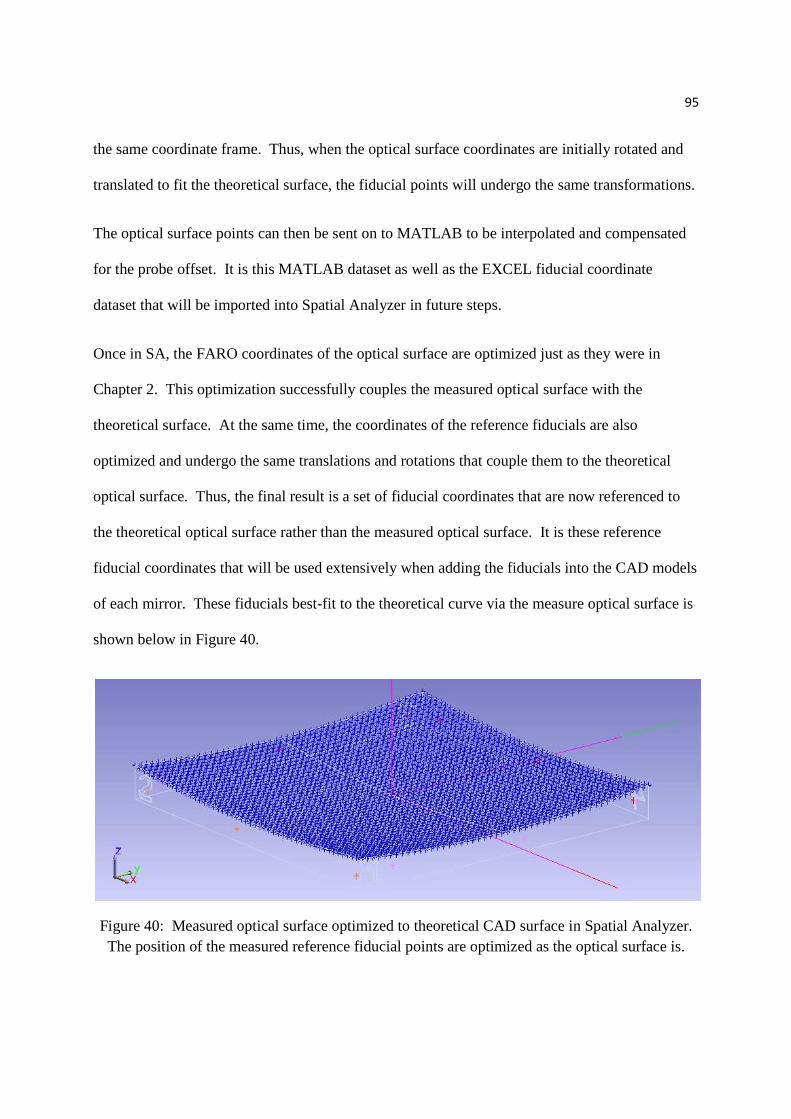
95
the same coordinate frame. Thus, when the optical surface coordinates are initially rotated and
translated to fit the theoretical surface, the fiducial points will undergo the same transformations.
The optical surface points can then be sent on to MATLAB to be interpolated and compensated
for the probe offset. It is this MATLAB dataset as well as the EXCEL fiducial coordinate
dataset that will be imported into Spatial Analyzer in future steps.
Once in SA, the FARO coordinates of the optical surface are optimized just as they were in
Chapter 2. This optimization successfully couples the measured optical surface with the
theoretical surface. At the same time, the coordinates of the reference fiducials are also
optimized and undergo the same translations and rotations that couple them to the theoretical
optical surface. Thus, the final result is a set of fiducial coordinates that are now referenced to
the theoretical optical surface rather than the measured optical surface. It is these reference
fiducial coordinates that will be used extensively when adding the fiducials into the CAD models
of each mirror. These fiducials best-fit to the theoretical curve via the measure optical surface is
shown below in Figure 40.
Figure 40: Measured optical surface optimized to theoretical CAD surface in Spatial Analyzer. The position of the measured reference fiducial points are optimized as the optical surface is.

96
4.5.Modeling Mirrors and Reference Fiducials in SolidWorks
Fortunately CAD models already exist for these mirrors based on the work that was done
previously. All that remains to be done is to add the reference fiducials to make these models
complete. At this point, these reference fiducials should have undergone the same rotations and
translations that were done to the measured and optimized FARO dataset of the optical surface.
These coordinates are now to be entered manually into the Assembly file of the M7 mirror. The
reason these need to be inserted into the Assembly file is because it uses the coordinate system
where the center point of the mirror has coordinates (0,0,0) as shown in Figure 18. To insert
these coordinates, a 3D sketch is to be created with points placed near the mirror in space. Then,
the correct coordinates are entered individually. Once this has been done in the Assembly file,
the same points must be made in the Part file of the mirror. These points should be made
coincident to the points made in the Assembly file. Though they are the same in relation to the
mirror, they have different coordinates as the Part file coordinate system is back in use. These
new reference fiducial points are shown on the CAD mirror below in Figure 41.
Figure 41: Reference fiducial points inserted into CAD model of mirror

97
As can be seen from Figure 41, there are 12 points that have been manually entered into this
CAD model, one for each fiducial. Because the FARO Arm takes data from the center of its
probe, this point represents the center of the probe as it is positioned in the fiducial, rather than
the actual depth of the fiducial. This is important to note and will be discussed in greater detail
later on.
Next, the appropriate side lengths are modeled using the exported Relationship files from Spatial
Analyzer. While working in the SolidWorks Part file, a small line should be created with one
end coinciding with the reference fiducial point. This line should be normal to the side of the
mirror the fiducial is machined into and should be the length shown in the Spatial Analyzer
Relationship file. As shown in Figure 39, the distance values to use for the length of this line are
circled in red. These values are the distance between each reference fiducial coordinate and the
plane representing the side of the mirror. An additional line should be created that is
perpendicular to the first. This line can be of any length and will be used to identify the correct
placement of the mirror edge in relation to the reference fiducials. The CAD model of the mirror
with these new lines is shown below in Figure 42.
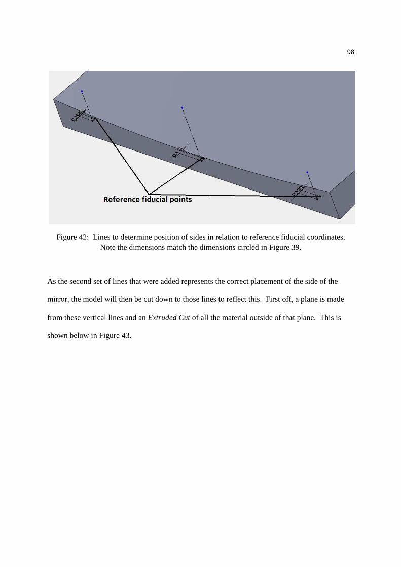
98
Figure 42: Lines to determine position of sides in relation to reference fiducial coordinates. Note the dimensions match the dimensions circled in Figure 39.
As the second set of lines that were added represents the correct placement of the side of the
mirror, the model will then be cut down to those lines to reflect this. First off, a plane is made
from these vertical lines and an Extruded Cut of all the material outside of that plane. This is
shown below in Figure 43.

99
Figure 43: The model of the CAD mirror being cut down to its correct side length based on distance from reference fiducials.
Once this mirror has been cut down to the correct size, the side length should be verified. This is
to ensure that the distance between the reference fiducial and the plane created was correct. If
the mirror ends up being 3mm too long in side length, then it’s possible that Spatial Analyzer
projected the coordinate that was taken in the reference fiducial to the surface of the probe, rather
than at the center where it is normally taken. There are a number of settings in Spatial Analyzer
that can force this projection, though it is not usually desired. If it is found that the mirror is too
large by 3mm, then the distances from the fiducials to the sides should be decreased by the radius
of the probe, which in this case was 1.5mm.The depth of the mirror, which was roughly
determined earlier, is left approximate as it has no value in the alignment process.
Next, the cones of each fiducial are created. This is done by using the fiducial point as the
bottom of the cone. Again, this is not how the fiducials are machined into the mirror in reality.

100
The result is that the cones in the CAD model will be shallower than reality. Though not
immediately intuitive, this is actually ideal because the bottom of the cone is now the location of
the center of the probe. When the mirror assembly alignment is being done later using Spatial
Analyzer and the FARO arm, the bottom of each cone is a tangible reference which can be
selected in Spatial Analyzer. The floating location where the center of the probe is could not be
selected in Spatial Analyzer if the cone depth in CAD matched reality. A mirror with the
fiducials correctly modeled is shown below in Figure 44.

101
Figure 44: SolidWorks model of mirror with correctly located fiducials
The last thing that needs to be done to the model of each mirror is to identify the optical center.
This center point is again taken from the Zemax prescription of the mirror. A 3D Sketch can be
used to insert this point and the coordinates for it can be entered. This should be done in the Part
file of the mirror as this uses the original coordinate frame. It is likely that the optical center of
the mirror is no longer at the geometric center of the mirror as was originally designed. In the
case of this example, the reason is that the surface of the mirror was not ideal. Thus, during the

102
optimization process, the best fit of the mirror to the theoretical curve reflected this. A line
should also be added which is normal to the surface of the mirror at the optical center point. This
will be used to align this mirror into the original CAD Assembly of the mirror array. This is the
final step of modeling a curved mirror. This should be repeated for any curved mirror in the
system.
4.5.1. Flat Mirrors
For flat mirrors, a much simplified procedure can be used. Recall the method which was
employed to measure the flat mirrors. First off, the coordinate system was relocated to one of
the corners of the mirror with the flat optical surface being one of the reference planes. Thus,
each reference fiducial coordinate will have a non-zero value in the direction normal to that
plane. This translates well to SolidWorks because this reference plane / optical surface can
immediately be created as one of the Front, Top, or Right planes. This plane can be made overly
large as the side lengths will be designated later. The reference fiducial points should then be
plotted individually based on the coordinates measured by the FARO Arm. Once these are in
place, the distance from each reference fiducial to that mirror side can be found using the
Relationship file that was exported from Spatial Analyzer. Creating the correct side lengths and
cone shapes is then done in the same way as it was for curved mirrors. An image of a completed
flat mirror is shown below in Figure 45.

103
Figure 45: Completed CAD model of a flat mirror
With a CAD model of each mirror in the mirror array completed, they are now ready to be
reentered into the original CAD Assembly.

104
4.6. Updating CAD Mirror Assembly with New Mirrors
The last step of this process is inserting the new, fiducial marked mirrors into the original CAD
mirror assembly. It is likely that a CAD assembly with the ideal mirror positions exists as
mechanical design for mounting these mirrors requires knowledge of mirror positions. If no
CAD assembly of mirror placements exists, it can easily be exported from ZEMAX and this
process can continue. The new, fiducial marked mirrors should be inserted to exactly overlay the
original mirror in the assembly. By doing this, the fiducial marked mirrors will be accurately
positioned based on the optical design. To accomplish this, the new mirrors should be placed
with their optical center at the position of the original optical center, which was the geometrical
center of the mirror. Thus the fiducial marked mirrors are overlaid on top of the original mirrors
in the mirror assembly. To correctly orient each mirror, the optical axes of the fiducial marked
and original mirrors should be aligned. For the powered mirrors, additional axes should be
aligned to fully constrain their position. A .STEP file is then created of the mirror array which is
later exported into Spatial Analyzer to prepare for the alignment procedure. This .STEP file is
shown below in Figure 46.

105
Figure 46: .STEP model of updated mirrors correctly positioned in CAD mirror assembly

106
4.7. Using FARO Arm and Spatial Analyzer to Align THz Mirrors
Before Spatial Analyzer and the FARO Arm can be used to align the mirror array, a 0th order
alignment of the mirrors should be completed. This 0th order alignment is done using non
stretching string, such as waxed floss or fishing wire, to correctly space the 4 corners of each
mirror. In the case of SuperCam, there are 7 mirrors that reside within the Optical Support
Structure (OSS). These mirrors serve as relay optics to transmit light to the focal plane array,
which resides within a cryostat. This cryostat thus becomes the initial reference used for
alignment. The first rough alignment must then be from the cryostat to the last mirror in the
SuperCam relay optics system, M7. This is a crucial alignment that is done without the use of
alignment tools. The result is that M7 could be incorrectly placed in the OSS which would in
turn position all of the other mirrors in the optical system incorrectly in reference to the OSS.
Thus, this first mirror should be carefully positioned. In addition to the 0th order alignment, the
CAD model can be used to provide additional references to how the mirror is positioned in the
OSS. In the case of the SuperCam OSS, there are enough degrees of freedom when mounting
each mirror that even a slight tilt of M7 can be accounted for by the remaining mirrors. It should
also be noted that in the final orientation at the SMT, the relative positioning between the OSS
and cryostat can be adjusted. This will be necessary to realign M7 to the cryostat during final
alignment.
With M7 being roughly aligned to the cryostat, M7 now becomes the reference surface. Moving
through the mirror array, M6 is then aligned to M7. This is again done using lengths of floss that
will provide the correct spacing between the corners of each mirror. This procedure should be
continued until each of the 7 mirrors is aligned to the mirror before it. Much in the same way
M7 is aligned to the cryostat, M1 will be aligned to the secondary mirror of the telescope. Some

107
minor adjustments in the mounting of the OSS will be made to adequately couple to the
telescope. It should be noted that the errors associated with this 0th order alignment are
cumulative: incorrect placement of a preceding mirror will translate into the next mirror. This
kind of cumulative alignment error will not be present during the final alignment with the FARO
Arm.
Once the 0th order alignment is completed, the FARO Arm is mounted near the OSS. The ideal
position is one in which the Arm’s probe can reach at least 3 reference fiducials on each mirror
in the system. This position is most likely centered very near the front of the OSS. It should be
mounted on a very stable base to prevent it from moving between measurements.
FARO Arm and Spatial Analyzer can now be used to improve the alignment of each mirror. To
begin with, a new SA file is to be opened and the FARO Arm instrument is loaded. This new
instrument is placed arbitrarily within the SA file. Next, the CAD model of the mirror array is
imported. This mirror array will be positioned so that the origin of the .STEP file coincides with
the origin of the new SA file. The result is that the instrument and the mirror array are not
positioned correctly in relation to one another. This is shown below in Figure 47.
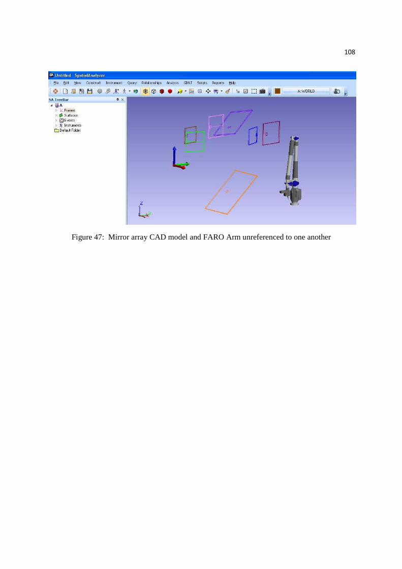
108
Figure 47: Mirror array CAD model and FARO Arm unreferenced to one another

109
4.7.1. Aligning FARO Arm to First THz Mirror
As an essential step in this alignment procedure, the position of the FARO Arm in relation to the
CAD array should be identical in the SA file as well as in reality. To accomplish this in SA, the
accessible reference fiducials on mirror M7 should be measured with the FARO Arm. In this
example, only 3 sides of fiducials were accessible for mirror M7. These measured points are
shown in Figure 48.
Figure 48: Reference fiducial points created in SA. These points are not yet aligned to mirror M7.
As can be seen in Figure 48, the measured reference fiducial points are nowhere near M7, which
is shown colored in green. Before these points can be referenced to the CAD model, the
projection offsets should be eliminated. This will prevent SA from correcting for a probe offset.
This is done by right clicking on each individual point in the SA TreeBar and selecting

110
Properties. Then in the Targeting Offsets box at the bottom, the values for Planar and Radial
offsets should be set to zero.
Next a set of reference points should be generated in SA. Select Construct -> Point(s) -> Layout
-> On Object Vertex By Clicking. This function allows the user to create points on the CAD
model of the mirror at a vertex. Points should be created at each of the reference fiducials that
were measured in the last step.
To align these points to the CAD model of M7, select Analysis -> Best-Fit Transformation ->
Points to Points. This function will be used to move the instrument in relation to the CAD
model by mating the points taken with the FARO Arm with the reference points of the mirror
generated in SA. Spatial Analyzer asks which points are reference points and which are
corresponding points. A pop up window titled Best-Fit Transformation then appears, as shown
below in Figure 49.
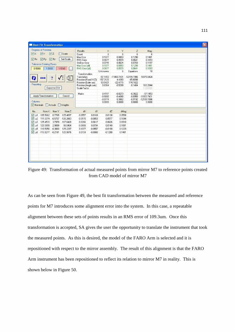
111
Figure 49: Transformation of actual measured points from mirror M7 to reference points created from CAD model of mirror M7
As can be seen from Figure 49, the best fit transformation between the measured and reference
points for M7 introduces some alignment error into the system. In this case, a repeatable
alignment between these sets of points results in an RMS error of 109.3um. Once this
transformation is accepted, SA gives the user the opportunity to translate the instrument that took
the measured points. As this is desired, the model of the FARO Arm is selected and it is
repositioned with respect to the mirror assembly. The result of this alignment is that the FARO
Arm instrument has been repositioned to reflect its relation to mirror M7 in reality. This is
shown below in Figure 50.
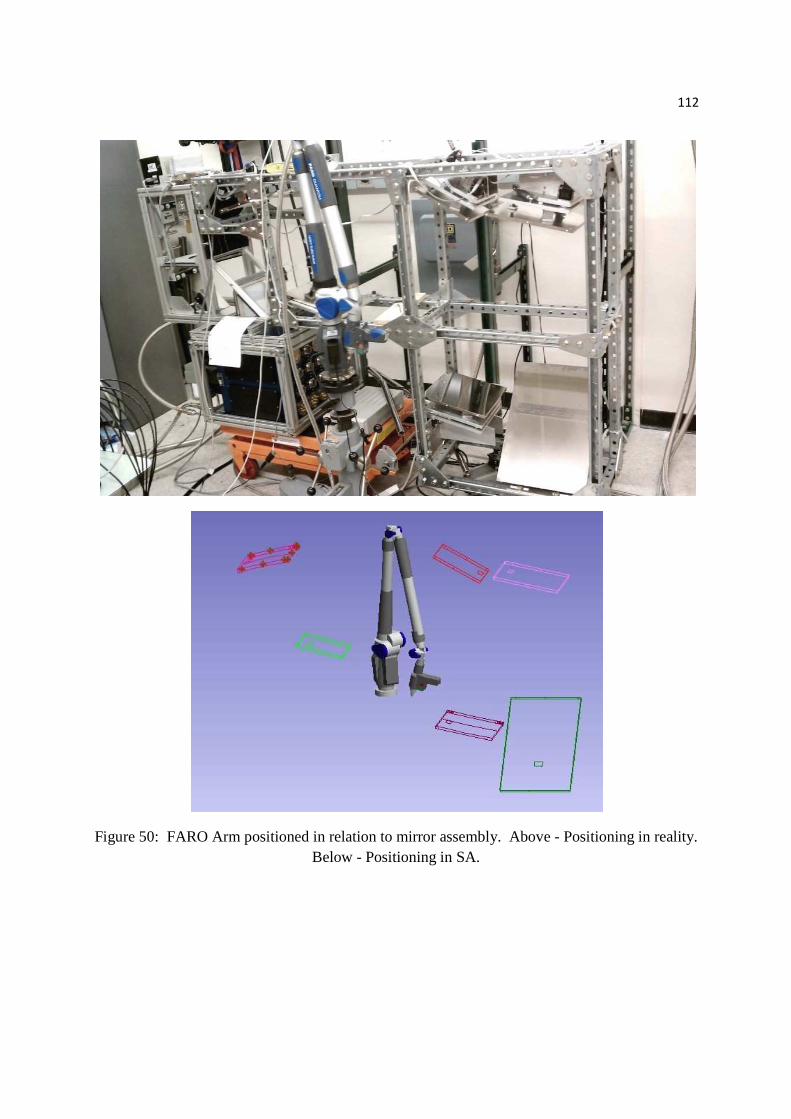
112
Figure 50: FARO Arm positioned in relation to mirror assembly. Above - Positioning in reality. Below - Positioning in SA.

113
4.7.2. Aligning Remaining Mirrors in System
With the dewar roughly positioned to M7 and the FARO Arm aligned to it as well, mirror M7
has become the reference mirror in which all the other mirrors will be aligned. This helps to
minimize cumulative errors as each mirror is aligned to M7, not the mirror before it. Recall the
earlier concern that the first mirror was positioned with some erroneous tilt within the OSS. This
is now a good time to take some quick reference fiducial measurements of the remaining mirrors
in the system to see if they are in a position where they can be adequately aligned.
Once this is complete, the reference fiducials are again used to align the remaining mirrors. It
makes no difference which mirror is aligned next. In this example, the mirrors will be aligned in
reverse order, from M6 to M1. When aligning M6, three accessible reference fiducials should be
measured with the FARO Arm. These points fully constrain the position of M6. Next, virtual
reference points should be created in Spatial Analyzer by selecting Construct -> Point(s) ->
Layout -> On Object Vertex By Clicking. The bottom of the reference fiducial cone in SA
should be selected and a reference point will be made there. The reference points created should
coincide with the fiducials that will be measured using the FARO Arm. These new virtual points
are then compared to the corresponding measured points. It should be noted that virtual points
represent the position of the CAD / theoretical mirror and the measured points represent the
position of the real mirror in the OSS. To determine the distance between virtual and measured
points, select Query -> Points to Points. This will display a window as shown in Figure 51
below.

114
Figure 51: Inter-Point Distance chart showing the distances between the measured points and the theoretical reference points. The values surrounded by green boxes display this distance in millimeters. It should be noted that this is the overall magnitude of the distance between
measured and theoretical. Individual X, Y, and Z components can also be displayed.
This query provides feedback which is used to more accurately position the mirror. The position
of the mirror should be adjusted to minimize the difference in position of the theoretical and
measured points. This is an iterative process where adjustments are made and then the points
are re-measured. Based on how well the new position fits to the CAD model position of the
mirror, further adjustments may be needed. This process is then repeated for each of the
remaining mirrors in the array. Table 9 below shows the final positioning of mirror M6.
Table 9: Distance between measured and reference points for final positioning of mirror M6. Units are in millimeters
X Y Z Mag P1 -0.063 -0.235 -0.132 0.277 P2 -0.018 -0.009 -0.100 0.102 P3 0.161 0.011 0.077 0.179
As can be seen, the positioning of the 3 reference fiducials in relation to theory is within the
tolerances established by the Monte Carlo tolerance analysis. The tolerance required for
translation in X, Y, Z was 1mm, while rotational tolerances required 0.1 degrees. Recall that the
rotational tolerance was dependent upon the footprint of the mirror. As M6 is the smallest mirror

115
is the assembly, it requires the tightest measurement accuracy for tip and tilt. It was found in the
tolerance analysis that points impacting tip and tilt must be positioned to within 176um. As Z is
the direction parallel with the optical axis, the largest positioning error for one of these points
was 132um, meeting the required tolerance.
An alignment test can be useful at this point to verify how well the mirrors are aligned. A laser
can be mounted at the telescope focus to observe how the beam is reflected. This can be used as
a crude alignment test. Though it has been determined that using the FARO Arm and this
procedure is adequate for mirror alignment, a laser tracker may be a way to improve alignment
even further.

116
4.8. Considering Procedural Alignment Errors
The final product of this alignment with FARO Arm is an assembly of mirrors that have been
best fit to their theoretical positions. The limit to the accuracy of this alignment technique is a
combination of errors. These errors include:
• Uncertainty in FARO Arm measurements when taking position coordinates of reference
fiducials for modeling in CAD
• Errors in surface modeling in MATLAB
• Best fitting the measured dataset to the theoretical dataset in Spatial Analyzer
• Aligning the FARO Arm to M7 using a Points to Points transformation
• Uncertainty in FARO Arm measurements when taking position coordinates of reference
fiducials for mirror alignment
• Error in the final position of the three reference fiducials. This is limited by the
resolution of the available mirror adjustment tools (stepper motor / micrometer /
differential screw)
Based on the result from Chapter 1, it has been found that the errors introduced through the
measurement uncertainty of the FARO Arm are very small in relation to the required tolerances
of the optical system. These alignment errors are less than 10um in translation directions and
less than 0.0065 degrees in rotation. The surface fitting procedure used in MATLAB provides
an RMS error of less than 5um. The next source of error is from the best-fit optimization of the
measured FARO data to the theoretical CAD surface in SA. As mentioned in the error analysis
for verifying surface figure in Chapter 2, the procedural error associated with this transformation
is difficult to quantify. Though this optimization process certainly introduces some error, it is
unfortunately bundled into the one fabrication RMS error value. For this analysis, it will again

117
be assumed that the error in the optimization itself is less than the 20-25um RMS of fabrication
error that was calculated. This error is not negligible but it is small in relation to the accepted
mirror position tolerances. The largest source of error is during the alignment itself. The initial
fitting of the FARO Arm to mirror M7 introduces an RMS error of 109.3um. This is an
inescapable source of error that is unfortunately compounded when aligning the remaining
mirrors in the system. Next, the uncertainty in mirror positioning based on the measurement
accuracy of the FARO Arm is accounted for again. This time, it is a result of taking
measurements of each reference fiducial. The final source of error is in regards to how well the
measured reference fiducials are aligned to the theoretical reference fiducials. In theory, this can
be done perfectly, which would produce no additional error. In practice, some error will of
course be introduced here. Fortunately, this error can be reduced by using mirror adjustment
tools that have excellent resolution. This will help to improve the positioning of the measured
reference fiducials to their theoretical positions. In this analysis, the value from the actual
alignment, 132um will be used.
Considering the combined effect of these errors, there is value in making a reasonable estimate
of the combined procedural errors. This is again done by taking the square root of the sum of the
squares of each error in this procedure. This is done because each error can be considered
independent of the other errors and is thus should not simply be added together. It should be
noted that the error in alignment of the reference fiducial points is not procedural and will not be
included in this calculation. This being said, a reasonable estimate for the procedural errors in
this system is shown below.
!10 + 5 + 25 + 109.3 + 10 + � = 176=�

118
This is not an insignificant amount of error for this procedure. Considering the error in fiducial
alignment, the total error in the position of the mirrors is 173.8um. In a situation where the
mirror is aligned perfectly, a total procedural error of 113.1um is calculated. Thus, by using
positioning tools with excellent resolution to minimize the distance between measured and
theoretical reference fiducials, the total error can be minimized down to as low as 113.1um. As
previously discussed, it is the tip and tilt of the smallest mirror in the SuperCam relay optics
system that requires the tightest alignment tolerance. According to the tolerance analysis in
Chapter 1, this tip / tilt tolerance translates to 176um of measurement accuracy. The cumulative
error in this procedure, including the actual positioning of M6, is very near the acceptable
threshold for aligning this mirror in that degree of freedom. An alignment of 132um in the Z
direction for the fiducials that determine tilt in M6 should thus be considered a maximum
alignment error that can be allowed. As the remaining alignment tolerances in the system require
less measurement accuracy, the errors in this procedure are acceptable. Thus, it has been
concluded that the FARO Arm and this procedure are capable of adequately aligning mirrors for
a submillimeter astronomy application. The combined effect of these errors is near, but within
the accepted tolerance for tip and tilt of the mirror and are very acceptable for the remaining
degrees of freedom.

119
5. Conclusions from Surface Characterization and Alignment Procedures
THz optics indeed provide some unique challenges when it comes to verifying their surface
figure and aligning them. One of the welcome characteristics of THz optics is that they do not
need a reflective surface. They can thus be made at less cost in comparison to optics that require
polishing. The downside of the lack of a reflective surface is that optical methods for
determining surface figure and alignment cannot be used. This scenario requires that an
alternative procedure be developed and used. The hypothesis of this thesis is thus restated:
Using an articulated metrology arm, coordinate data processing, and optical design
software, the surface figure of non-reflective THz optics can be verified and its resulting
effect on the optical system can be determined.
Through the use of an articulated metrology arm and mechanical reference fiducials, non-
reflective THz optics can be aligned within the alignment tolerances required of the system.
Through the course of this thesis, these postulates have been tested and verified. These are the
results for each of the procedures that have been developed.

120
5.1. Verifying the Surface Figure of a THz Optic
It was found that an articulated metrology arm could be used to measure the surface of a THz
optic. This measured surface data was then imported into MATLAB where it was interpolated
and corrected for the probe radius offset of the FARO Arm probe. This correctly dataset was
then returned to Spatial Analyzer where it underwent a best-fit transformation with a theoretical
surface of the mirror being analyzed. This best-fit transformation was accomplished by
minimizing the differences between the measured and theoretical surfaces. This difference
between the two thus represents the fabrication error of the THz mirror. This fabrication error
was then plotted and analyzed. Figure 28 shows this error for mirror M7.
After analyzing what this plot physically represents, it was determined that the radius of
curvature of the mirror was fabricated to be larger than what it should have been in theory.
The two questions that were asked in the Introduction can now be revisited:
• How accurately was the optical surface fabricated?
• How do the fabricated optical surfaces affect the optical performance of the system?
Table 3 below compares how accurately each of the powered optical surfaces, M4 and M7 were
fabricated.
Table 3: Fabrication error of SuperCam powered mirrors, M4 and M7. All units in um.
RMS Error P-V Error
M4 21.1 110.5
M7 26.5 131.5

121
It was determined that neither mirror was fabricated perfectly. The resulting effect on the overall
optical performance of the system would provide the feedback on whether or not they were
adequate for the SuperCam relay optics.
This was accomplished through the use of Zernike polynomials. The dataset of differences
between measured and theoretical surfaces was imported into a MATLAB script that
decomposed the dataset into coefficients for a set of Standard Zernike polynomials. These
coefficients thus represented the fabrication error of the surface, which could now be reentered
into ZEMAX. This was done with both M4 and M7 and the resulting effect of the overall optical
performance was determined. The OPDs of the optical system before and after the fabricated
surfaces were reentered into ZEMAX are shown in Figure 35.
The final conclusion was that though both powered mirrors were not made perfectly, the overall
effect on the optical performance was acceptable. Before the actual surfaces were reentered into
ZEMAX, the RMS wavefront error was ���. After the as-built surfaces were entered, this
wavefront error increased to �� . �. This was deemed a very acceptable amount of error as the
threshold for acceptance was ��.
The procedural errors of the system were also calculated. Though an exact value could not be
determined, a reasonable estimate of total procedural error is 37.9um. This was considered small
enough to not have a significant impact on the accuracy of the surface figure characterizing
procedure.

122
It was thus found that the proposed procedure for verifying the surface figure of a THz optic was
successful. The results of the actual surface figures of the powered mirrors as well as their effect
on the overall optical performance were both logical and reasonable.

123
5.2. Aligning THz Optics
It was found that by using an articulated metrology arm, the surface of the optic could be
measured at the same time a set of mechanical reference fiducials. These reference fiducials
were designed to fully constrain the top of the FARO Arm probe so that repeatable
measurements could be taken. These reference fiducial positions were measured. Next, a best fit
transformation was used to couple the measured optical surface to the theoretical surface of the
mirror. The result was that the reference fiducials were now related to the theoretical optical
surface. They were then incorporated into the CAD model of the mirror. After each mirror had
its reference fiducials modeled, they were mated back into the original CAD model of the mirror
system. The assembly of the final positioning of the new mirror models was then exported from
SolidWorks and into Spatial Analyzer. It was this assembly that was used as a theoretical
positioning for each mirror. The FARO Arm was then aligned to the first mirror of the system.
At this point, each preceding mirror is then aligned to the first mirror using 3 reference fiducials
from each mirror. Using the built in adjustments for each mirror, an iterative process is used to
minimize the distance between the actual measured position of the reference fiducials and where
those fiducials should be in theory.
The two questions that were asked in the Introduction can now be revisited:
• How accurately is each optic aligned?
• Is this alignment adequate for the performance of this system?
The accuracy of the alignment of each optic is easily determined at this point. A point to point
query in Spatial Analyzer produces a table like the one shown in Table 9.
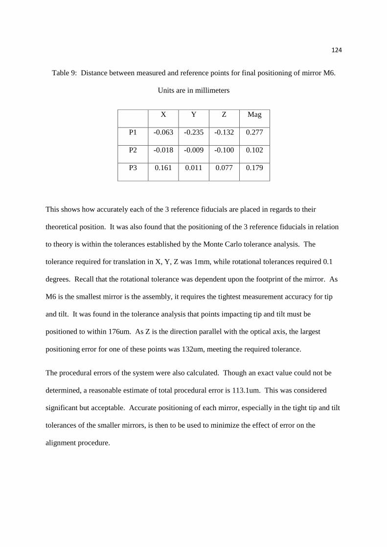
124
Table 9: Distance between measured and reference points for final positioning of mirror M6.
Units are in millimeters
X Y Z Mag
P1 -0.063 -0.235 -0.132 0.277
P2 -0.018 -0.009 -0.100 0.102
P3 0.161 0.011 0.077 0.179
This shows how accurately each of the 3 reference fiducials are placed in regards to their
theoretical position. It was also found that the positioning of the 3 reference fiducials in relation
to theory is within the tolerances established by the Monte Carlo tolerance analysis. The
tolerance required for translation in X, Y, Z was 1mm, while rotational tolerances required 0.1
degrees. Recall that the rotational tolerance was dependent upon the footprint of the mirror. As
M6 is the smallest mirror is the assembly, it requires the tightest measurement accuracy for tip
and tilt. It was found in the tolerance analysis that points impacting tip and tilt must be
positioned to within 176um. As Z is the direction parallel with the optical axis, the largest
positioning error for one of these points was 132um, meeting the required tolerance.
The procedural errors of the system were also calculated. Though an exact value could not be
determined, a reasonable estimate of total procedural error is 113.1um. This was considered
significant but acceptable. Accurate positioning of each mirror, especially in the tight tip and tilt
tolerances of the smaller mirrors, is then to be used to minimize the effect of error on the
alignment procedure.

125
It was thus found that the proposed procedure for aligning THz optics with an articulated
metrology arm was successful. The feedback received in regards to the position of each
reference fiducial is adequate to iterate on the position of the mirror. It was also found that the
FARO Arm was capable of measurement accuracies well within the alignment tolerances of the
optical system. These tolerances were also useful in determining if the mirror had been aligned
to an acceptable accuracy.
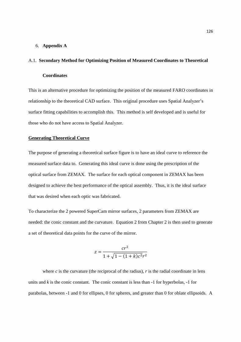
126
6. Appendix A
A.1. Secondary Method for Optimizing Position of Measured Coordinates to Theoretical
Coordinates
This is an alternative procedure for optimizing the position of the measured FARO coordinates in
relationship to the theoretical CAD surface. This original procedure uses Spatial Analyzer’s
surface fitting capabilities to accomplish this. This method is self developed and is useful for
those who do not have access to Spatial Analyzer.
Generating Theoretical Curve
The purpose of generating a theoretical surface figure is to have an ideal curve to reference the
measured surface data to. Generating this ideal curve is done using the prescription of the
optical surface from ZEMAX. The surface for each optical component in ZEMAX has been
designed to achieve the best performance of the optical assembly. Thus, it is the ideal surface
that was desired when each optic was fabricated.
To characterize the 2 powered SuperCam mirror surfaces, 2 parameters from ZEMAX are
needed: the conic constant and the curvature. Equation 2 from Chapter 2 is then used to generate
a set of theoretical data points for the curve of the mirror.
� = A> 1 + !1 − (1 + \,A >
where c is the curvature (the reciprocal of the radius), r is the radial coordinate in lens
units and k is the conic constant. The conic constant is less than -1 for hyperbolas, -1 for
parabolas, between -1 and 0 for ellipses, 0 for spheres, and greater than 0 for oblate ellipsoids. A
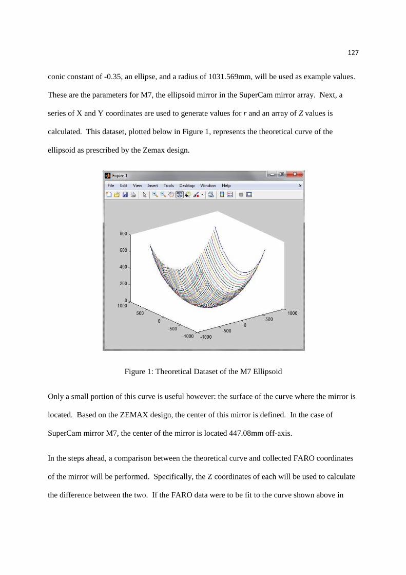
127
conic constant of -0.35, an ellipse, and a radius of 1031.569mm, will be used as example values.
These are the parameters for M7, the ellipsoid mirror in the SuperCam mirror array. Next, a
series of X and Y coordinates are used to generate values for r and an array of Z values is
calculated. This dataset, plotted below in Figure 1, represents the theoretical curve of the
ellipsoid as prescribed by the Zemax design.
Figure 1: Theoretical Dataset of the M7 Ellipsoid
Only a small portion of this curve is useful however: the surface of the curve where the mirror is
located. Based on the ZEMAX design, the center of this mirror is defined. In the case of
SuperCam mirror M7, the center of the mirror is located 447.08mm off-axis.
In the steps ahead, a comparison between the theoretical curve and collected FARO coordinates
of the mirror will be performed. Specifically, the Z coordinates of each will be used to calculate
the difference between the two. If the FARO data were to be fit to the curve shown above in

128
Figure 1, then the difference in the Z direction is not normal to the surface of the curve. This is
not an ideal comparison for the fit optimization process used in later steps. Thus, the curve is to
be rotated so that the normal at the center point of the mirror is collinear with the Z-axis. The
necessary rotation was determined by calculating the slope at the center point and rotating by
that angle in the opposite direction. The location of the mirror’s center point is then translated so
that its coordinates are (0,0,0). These transformations were done using rotation matrices and
X,Y,Z offsets in an EXCEL spreadsheet. . A cross section of the mirror undergoing this rotation
and translation is shown below, which is Figure 17 from Chapter 2.
Figure 17: Rotation and translation to orient the center point of the mirror
Now that the theoretical curve has been rotated and translated, the equation of that curve has
changed. An equation for this new curve will be needed later to generate Z coordinates at the
appropriate (X, Y) positions. To create this equation, the Surface Fitting Tool in MATLAB is to
be used.
The Surface Fitting Tool, called in MATLAB using the command sftool, provides a means of
generating a surface and equation for a dataset. Once the Surface Fitting Tool is opened, the X,
-150
-100
-50
0
50
100
150
200
-200 0 200 400 600 800Y-A
xis
(m
m)
X-Axis (mm)
Orienting the Center of the Mirror
Original
Rotated
Translated

129
Y, Z data from the rotation and translation EXCEL spreadsheet is entered. The type of surface
fit is then selected. Because a usable equation is desired, Polynomial is selected from the surface
fit type drop down menu. The order of that polynomial in both the X and Y directions can be
selected. A higher order will improve the accuracy of the surface fit in this case. Thus, 5th order
is selected for both X and Y axes. The form of this equation is as follows:
Equation 1
<=>?@AB ?)CC)DE BF=@C)GD= H�� + (H�� ∗ , + (H�� ∗ �, + (H � ∗ , + (H�� ∗ ∗ �, + (H� ∗ � ,+ (H�� ∗ �, + (H � ∗ ∗ �, + (H� ∗ ∗ � , + (H�� ∗ ��, + (H�� ∗ �,+ (H�� ∗ � ∗ �, + (H ∗ ∗ � , + (H�� ∗ ∗ ��, + (H�� ∗ ��, + (H�� ∗ �,+ (H�� ∗ � ∗ �, + (H� ∗ � ∗ � , + (H � ∗ ∗ ��, + (H�� ∗ ∗ ��, + (H��∗ ��,
with all the p subscript values being coefficients determined by MATLABs Surface
Fitting Tool.
In order to use this surface fit in MATLAB, a function must be created which can be called in
another MATLAB script. This is done by selecting File -> Generate Code. The appropriate
data must be entered into this function when it is called in MATLAB. The output for a 5th order
polynomial in both axes (X and Y) is an equation with 21 coefficients. The equation and the
coefficients are displayed in the MATLAB Command Window when the surface fitting function
is run.
The accuracy of the fit is again represented by the RMS Error (RMSE) which is displated in the
Surface Fitting Tool window.
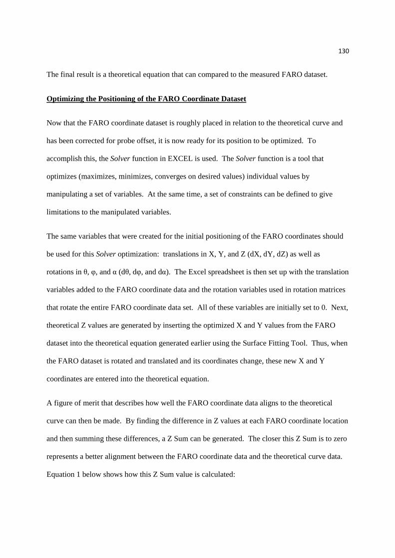
130
The final result is a theoretical equation that can compared to the measured FARO dataset.
Optimizing the Positioning of the FARO Coordinate Dataset
Now that the FARO coordinate dataset is roughly placed in relation to the theoretical curve and
has been corrected for probe offset, it is now ready for its position to be optimized. To
accomplish this, the Solver function in EXCEL is used. The Solver function is a tool that
optimizes (maximizes, minimizes, converges on desired values) individual values by
manipulating a set of variables. At the same time, a set of constraints can be defined to give
limitations to the manipulated variables.
The same variables that were created for the initial positioning of the FARO coordinates should
be used for this Solver optimization: translations in X, Y, and Z (dX, dY, dZ) as well as
rotations in θ, φ, and α (dθ, dφ, and dα). The Excel spreadsheet is then set up with the translation
variables added to the FARO coordinate data and the rotation variables used in rotation matrices
that rotate the entire FARO coordinate data set. All of these variables are initially set to 0. Next,
theoretical Z values are generated by inserting the optimized X and Y values from the FARO
dataset into the theoretical equation generated earlier using the Surface Fitting Tool. Thus, when
the FARO dataset is rotated and translated and its coordinates change, these new X and Y
coordinates are entered into the theoretical equation.
A figure of merit that describes how well the FARO coordinate data aligns to the theoretical
curve can then be made. By finding the difference in Z values at each FARO coordinate location
and then summing these differences, a Z Sum can be generated. The closer this Z Sum is to zero
represents a better alignment between the FARO coordinate data and the theoretical curve data.
Equation 1 below shows how this Z Sum value is calculated:
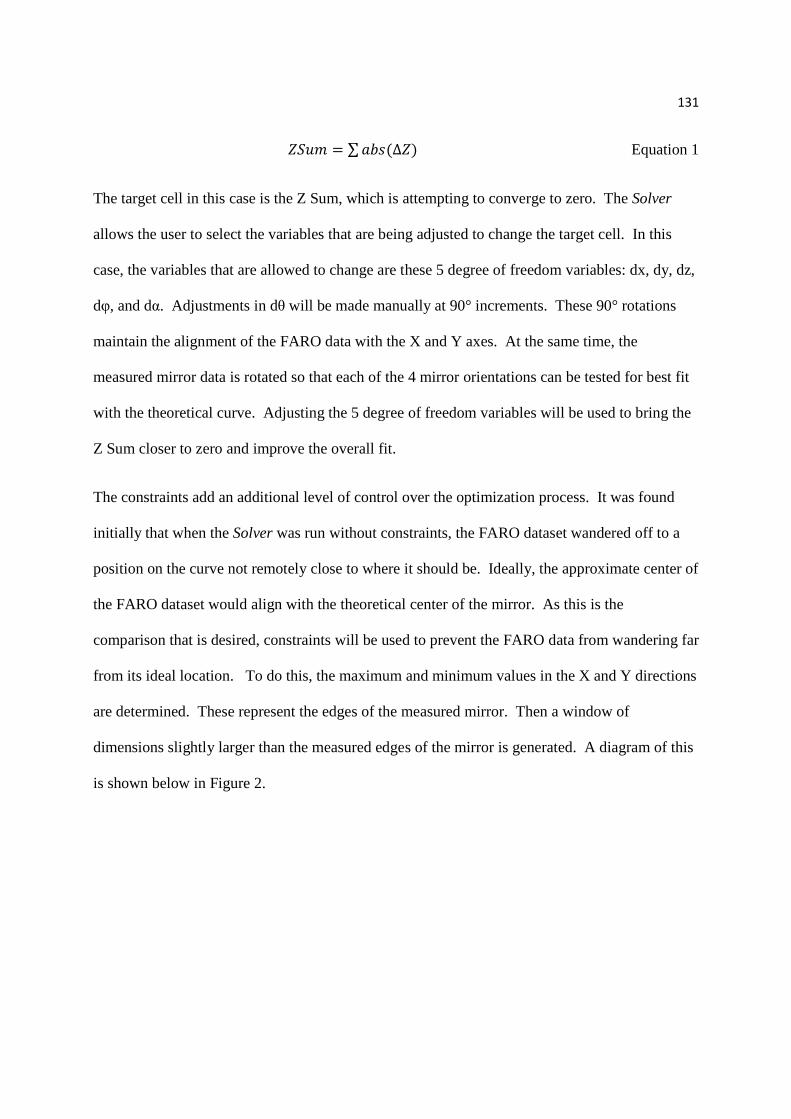
131
�<=� = ∑ @NR(∆�, Equation 1
The target cell in this case is the Z Sum, which is attempting to converge to zero. The Solver
allows the user to select the variables that are being adjusted to change the target cell. In this
case, the variables that are allowed to change are these 5 degree of freedom variables: dx, dy, dz,
dφ, and dα. Adjustments in dθ will be made manually at 90° increments. These 90° rotations
maintain the alignment of the FARO data with the X and Y axes. At the same time, the
measured mirror data is rotated so that each of the 4 mirror orientations can be tested for best fit
with the theoretical curve. Adjusting the 5 degree of freedom variables will be used to bring the
Z Sum closer to zero and improve the overall fit.
The constraints add an additional level of control over the optimization process. It was found
initially that when the Solver was run without constraints, the FARO dataset wandered off to a
position on the curve not remotely close to where it should be. Ideally, the approximate center of
the FARO dataset would align with the theoretical center of the mirror. As this is the
comparison that is desired, constraints will be used to prevent the FARO data from wandering far
from its ideal location. To do this, the maximum and minimum values in the X and Y directions
are determined. These represent the edges of the measured mirror. Then a window of
dimensions slightly larger than the measured edges of the mirror is generated. A diagram of this
is shown below in Figure 2.
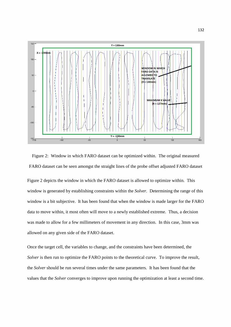
132
Figure 2: Window in which FARO dataset can be optimized within. The original measured
FARO dataset can be seen amongst the straight lines of the probe offset adjusted FARO dataset
Figure 2 depicts the window in which the FARO dataset is allowed to optimize within. This
window is generated by establishing constraints within the Solver. Determining the range of this
window is a bit subjective. It has been found that when the window is made larger for the FARO
data to move within, it most often will move to a newly established extreme. Thus, a decision
was made to allow for a few millimeters of movement in any direction. In this case, 3mm was
allowed on any given side of the FARO dataset.
Once the target cell, the variables to change, and the constraints have been determined, the
Solver is then run to optimize the FARO points to the theoretical curve. To improve the result,
the Solver should be run several times under the same parameters. It has been found that the
values that the Solver converges to improve upon running the optimization at least a second time.

133
Eventually the Z Sum value will be unchanged and the use of the Solver can be stopped. Figure
3 below is a screen shot of the Solver being used in the optimization process.
Figure 3: Solver optimization process
The final result of these Solver optimization runs is a FARO dataset that is best fit to the
theoretical surface of the optic that was measured. This is shown below in Figure 4.

134
Figure 4: Optimized fit of FARO data
It should be noted that this alignment process is not perfect. The error incorporated with this
alignment can be calculated by dividing the summed deltas between Z values by the number of
points in the data set. In the ellipsoid example, a total of 2500 points were used. With a Z Sum
value of 107.5, an error per point of 43um is calculated. This is an average error distributed
throughout all of the points. This is a comparable error to what was found in the Spatial
Analyzer method, which consistently calculated between 20 and 25um.
It has been found that this method is usable if Spatial Analyzer is not available. It is certainly a
more difficult and time consuming method, and also produces a larger alignment error. For this
reason, it is recommended that Spatial Analyzer be used if available.

135
References
Groppi, Christopher. “Test and integration results from SuperCam: a 64-pixel array receiver for the 350
GHz atmospheric window.” SPIE Millimeter, Submillimeter, and Far-Infrared Detectors and
Instrumentation for Astronomy V. 7741. (2010): Print.
Fricker, Paul. “Analyzing LASIK Optical Data Using Zernike Functions.” MATLAB Digest (2008): 1-6. Web.
2 Aug 2011.
<http://www.mathworks.com/company/newsletters/digest/2008/jan/zernike.html>.
“ZEMAX Optical Design Program.” User’s Manual. 2011.