Using a Parameterization of a Radiative Transfer Model to Build ...

Using a Parameterization of a Radiative Transfer Model to Build High-ResolutionMaps of Typical Clear-Sky UV Index in Catalonia, Spain

JORDI BADOSA, JOSEP-ABEL GONZÁLEZ, AND JOSEP CALBÓ

Departament de Física, Grup de Física Ambiental, Universitat de Girona, Girona, Spain

MICHIEL VAN WEELE

Royal Netherlands Meteorological Institute (KNMI), De Bilt, Netherlands

RICHARD L. MCKENZIE

National Institute of Water and Atmospheric Research (NIWA), Lauder, New Zealand

(Manuscript received 5 May 2004, in final form 22 November 2004)

ABSTRACT

To perform a climatic analysis of the annual UV index (UVI) variations in Catalonia, Spain (northeastof the Iberian Peninsula), a new simple parameterization scheme is presented based on a multilayerradiative transfer model. The parameterization performs fast UVI calculations for a wide range of cloudlessand snow-free situations and can be applied anywhere. The following parameters are considered: solarzenith angle, total ozone column, altitude, aerosol optical depth, and single-scattering albedo. A sensitivityanalysis is presented to justify this choice with special attention to aerosol information. Comparisons withthe base model show good agreement, most of all for the most common cases, giving an absolute errorwithin �0.2 in the UVI for a wide range of cases considered. Two tests are done to show the performanceof the parameterization against UVI measurements. One uses data from a high-quality spectroradiometerfrom Lauder, New Zealand [45.04°S, 169.684°E, 370 m above mean sea level (MSL)], where there is a lowpresence of aerosols. The other uses data from a Robertson–Berger-type meter from Girona, Spain (41.97°N,2.82°E, 100 m MSL), where there is more aerosol load and where it has been possible to study the effect ofaerosol information on the model versus measurement comparison. The parameterization is applied to a cli-matic analysis of the annual UVI variation in Catalonia, showing the contributions of solar zenith angle, ozone,and aerosols. High-resolution seasonal maps of typical UV index values in Catalonia are presented.

1. Introduction

Disseminating the actual levels of UV radiation hasrecently become very common so that the populationcan be informed and take precautionary measuresagainst the known harmful effects that this radiationcan produce on human beings (e.g., Vanicek et al.2000). For this purpose, the UV index (UVI)—an esti-mation of the UV levels that are important for theeffects on human skin—is the magnitude that is com-monly used. It is derived from the erythemal UV irra-diance (UVE), which is the integration of the mono-chromatic UV irradiance (280–400 nm) weighted by theCommission Internacionale de l’Eclairage (CIE) spec-tral action function (McKinlay and Diffey 1987). UVI is

a unitless magnitude that is defined as 40 times UVE(expressed in watts per meter squared).

UVI commonly takes values from 0 to 16 (reachingthe maximum in summer midday) but in some regionsand for particular conditions it can reach up to 20 units.Larger UVI values correspond to more harmful UVradiation for human beings. The overall effect dependson the exposed parts of the body, their sensitivity to UVradiation, and the dose received (information availableonline at http://www.who.int/).

The use of UVI maps is necessary to entirely cover aparticular region. However, there is usually a lack ofhigh-density spatial UVI measurements to represent allthe territory. So, other sources (such as meteorologicalground- and satellite-based information) and methods(such as empirical algorithms and radiative transfermodeling) usually become necessary.

Some authors have solved the lack of UVI ground-based measurements by combining UVE and total solarirradiance measurements, because the latter are moreoften measured than the former. Bodeker and McKen-

Corresponding author address: Jordi Badosa, Grup de FísicaAmbiental, Departament de Física, Universitat de Girona, EscolaPolitècnica Superior, Campus Montilivi, EPS II, 17071 Girona,Spain.E-mail: [email protected]

JUNE 2005 B A D O S A E T A L . 789

© 2005 American Meteorological Society

JAM2237

zie (1996) used radiative transfer modeling and empiri-cal relations between these two magnitudes to developan algorithm that retrieves UVI for all cloud condi-tions, considering total irradiance, total ozone column(TOZ), altitude, surface pressure, temperature, and hu-midity measurements. This algorithm is currently usedin the National Institute of Water and AtmosphericResearch (NIWA) UV Atlas project to produce mapsand time series of UVI over New Zealand (additionalinformation is available online at http://www.niwa.cri.nz/services/uvozone/atlas). Schmalwieser and Schau-berger (2001) established relationships between UVEmeasurements that are available from 9 sites and totalirradiance measurements that are available from 39other sites in Austria to cover the whole country. Cloudeffects were also included through relationships be-tween UVE and total irradiance. For the visualizationof the data, daily maps of noontime UVI were thencreated with a spatial resolution of approximately 1 km.Fioletov et al. (2003) found a statistical relationshipbetween total irradiance and UVE, considering totalozone, snow cover, dewpoint temperature, and altitude.They applied this algorithm to 45 stations with totalirradiance measurements in Canada to estimate a UVIclimatology. Different types of statistical maps wereproduced, such as monthly mean daily UVI, meannoontime UVI, 95th percentile of the noontime UVI,and hourly mean UVI.

Some other studies have produced UVI maps basedon radiative transfer modeling and using satellite mea-surements as input. For example, Verdebout (2000)presented a method to produce UVI maps over Europewith 0.05° spatial resolution and half an hour of poten-tial temporal resolution. The method is based on alookup table generated with a radiative transfer model,whose inputs are solar zenith angle (SZA), total ozone,cloud optical thickness, near-surface horizontal visibil-ity, altitude, and surface UV albedo.

Concerning satellite-derived information, daily UVdose maps and values are available worldwide from theTotal Ozone Mapping Spectrometer (TOMS) (see in-formation online at http://toms.gsfc.nasa.gov). The al-gorithm developed for these calculations uses a table ofsolutions of the radiative transfer equation. This tablealso serves for TOMS total ozone column retrievals andtakes into account cloud effect (assuming that cloudconditions at noontime are representative for the wholeday) and surface albedo, using a method to assess theprobability of snow presence.

Recently, Schmalwieser et al. (2002) presented amodel based on ground-based spectral measurementsthat calculates the spectral irradiance for 16 wave-lengths between 297.5 and 380 nm and used this model

to predict UVI worldwide (information online at http://i115srv.vu-wien.ac.at/uv_online.htm). The model takesinto account solar zenith angle, altitude, and forecastedtotal ozone. Allaart et al. (2004) developed an empiricalalgorithm to predict UVI (hereinafter called ALUVI)that takes into account solar zenith angle, total ozone,and altitude. Noontime-predicted worldwide UVImaps based on the assimilated Scanning Imaging Ab-sorption Spectrometer for Atmospheric Chartography(SCIAMACHY) total ozone measurements are pre-sented for a given day and the following 4 days at theTropospheric Emission Monitoring Internet Service(TEMIS) Web site (available online at http://www.temis.nl/uvradiation).

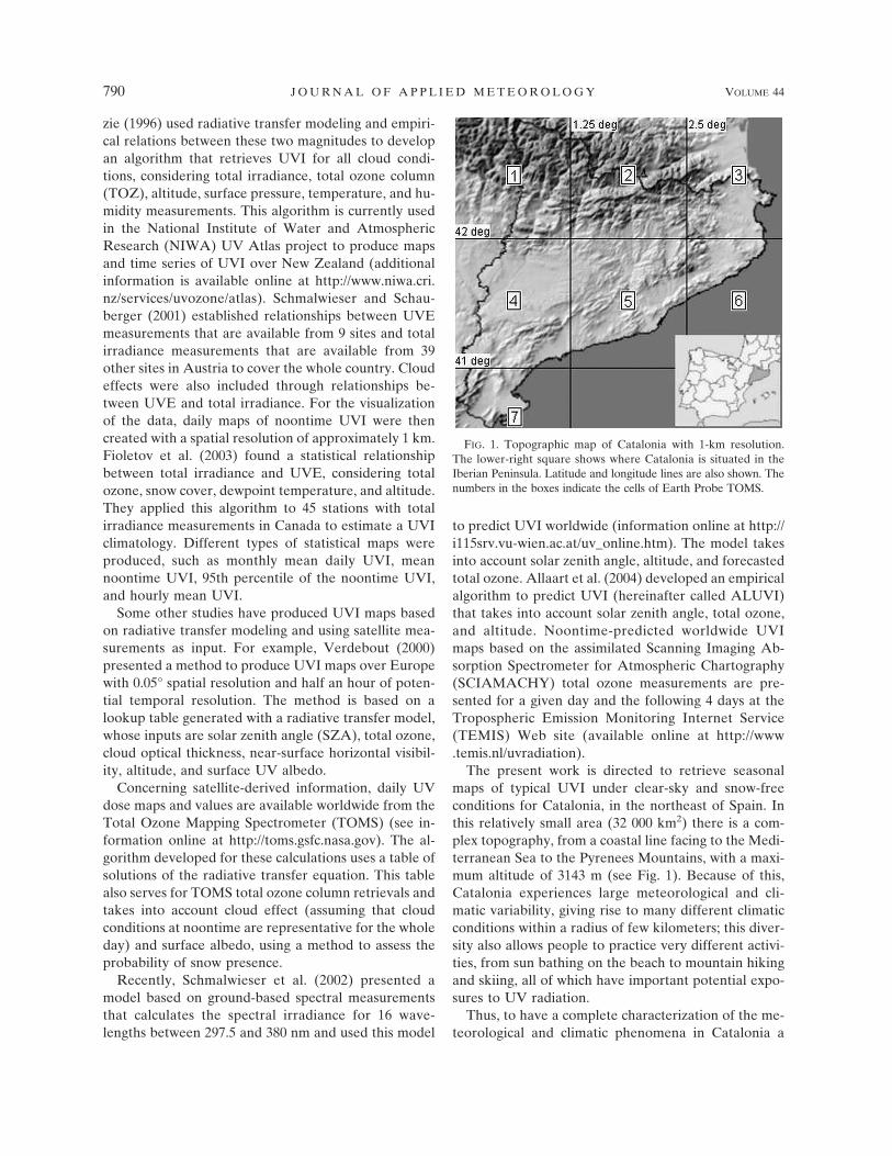
The present work is directed to retrieve seasonalmaps of typical UVI under clear-sky and snow-freeconditions for Catalonia, in the northeast of Spain. Inthis relatively small area (32 000 km2) there is a com-plex topography, from a coastal line facing to the Medi-terranean Sea to the Pyrenees Mountains, with a maxi-mum altitude of 3143 m (see Fig. 1). Because of this,Catalonia experiences large meteorological and cli-matic variability, giving rise to many different climaticconditions within a radius of few kilometers; this diver-sity also allows people to practice very different activi-ties, from sun bathing on the beach to mountain hikingand skiing, all of which have important potential expo-sures to UV radiation.

Thus, to have a complete characterization of the me-teorological and climatic phenomena in Catalonia a

FIG. 1. Topographic map of Catalonia with 1-km resolution.The lower-right square shows where Catalonia is situated in theIberian Peninsula. Latitude and longitude lines are also shown. Thenumbers in the boxes indicate the cells of Earth Probe TOMS.

790 J O U R N A L O F A P P L I E D M E T E O R O L O G Y VOLUME 44

large density of measuring sites is required. Currently,there are only five sites where erythemal UV irradianceis measured in Catalonia, all of which have a short datarecord. A possible alternative could be to retrieve typi-cal UVI values based on radiative transfer calculations.However, on the one hand, we want high spatial reso-lution coverage (which involves an important compu-tational cost) and, on the other hand, no accurate highlyresolved information about some input variables, suchas the aerosol information, is available. So it seems rea-sonable to simplify models through their parameteriza-tion, make assumptions, and then also allow fast calcu-lations. The parameterization here presented [namedthe Parameterization of the Tropospheric Ultravioletand Visible (PTUV) radiative transfer model] considersSZA, TOZ, altitude (z), aerosol optical depth at 368nm (AOD368) and aerosol single scattering albedo(SSA) as input parameters.

The PTUV model is introduced in section 2, includ-ing a discussion about the base model used, the choiceof the parameters, the mathematical structure of theformula, and, finally, comparisons with the base model.In section 3, the parameterization is tested by compar-ing it with UVI measurements from two sites—one us-ing high spectral UV measurements and the other froma Robertson–Berger-type meter. Special attention ispaid to the aerosol effects and how the aerosol infor-mation is introduced to the model. In section 4 theannual variations of SZA, TOZ, and AOD368, and howthey affect the annual UVI variation, is analyzed andthe process of generating seasonal UVI maps for Cata-lonia is explained.

2. Methodology

a. Radiative transfer calculations

The Tropospheric Ultraviolet and Visible (TUV) Ra-diative Transfer Model (Madronich 1993), version 4.1,is the base model for the parameterization. The pack-age, which consists of a group of routines written inFORTRAN77, is available online (see http://www.acd.ucar.edu/TUV/). TUV is a multilayer modelthat solves the radiative transfer equation by twostreams or discrete ordinates (DISORT) with nstreams. Versions with pseudospherical corrections areavailable. Because only plane irradiances are studied,the DISORT code with eight streams and pseudo-spherical corrections is used in this work.

The TUV default options have been considered here,except for changing the default aerosol optical depthfixed values from Elterman (1968) for a new aerosolprofile described below. The spectral range considered

for all UVI calculations was 280–400 nm, with a wave-length increment of 1 nm.

b. Parameters considered

Although the application discussed here is only forthe small region of Catalonia, the parameterization wasdeveloped in order to be able to explain a wide range ofconditions under cloudless skies. Because of this, SZA,TOZ, z, AOD368, and SSA were taken with wide ranges(as shown in Table 1).

However, some particular situations are omittedfrom the coverage of this study. Particular surface typeswith large albedo, such as snow and sand, are not takeninto account here. It is known that the effect of surfacealbedo on UVI depends on the topography, type of soil,and also the turbidity of the surroundings (e.g., Mad-ronich 1993; Madronich et al. 1994); this makes it dif-ficult to find the actual surface albedo values that rep-resent each site at each moment. Weihs et al. (2002)considered three inversion methods to retrieve surfacealbedo from UV measurements in spring in Germanyand surrounding areas. They found differences of �0.15in the albedo that is retrieved with the three methodsthat lead, according to the authors, to an uncertainty inthe UV irradiance calculation [in ultraviolet B (UVB)and ultraviolet A (UVA)] of approximately �3%–5%.In our study, there is a lack of information about cli-matic estimations of surface albedo and snow cover forCatalonia; because of this, considering large-albedocases would be too subjective and, thus, nonrepresen-tative of the real situation. Most common surfaces havesurface albedo less than 10% (e.g., Madronich 1993). Inthis work, a typical value of 5% is set constant for allthe UV calculations.

Also, the conditions of very high turbidity have notbeen considered for the retrieval of PTUV becausethese situations are rare (especially in Catalonia) and toparameterize them would add extra complexity.

In the following, the five parameters and their ranges

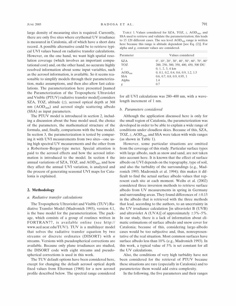
TABLE 1. Values considered for SZA, TOZ, z, AOD368, andSSA used to retrieve and validate the parameterization; this leadsto 15 120 different cases. The sea level AOD368 range is writtenhere because this range is altitude dependent [see Eq. (2)]. Foralpha and g, constant values are considered.

Parameter Values considered

SZA 0°, 10°, 20°, 30°, 40°, 50°, 60°, 70°, 80°TOZ 200, 250, 300, 350, 400, 450, 500 DUz 0, 1, 2, 3, 4 kmAOD368 0, 0.1, 0.2, 0.4, 0.6, 0.9, 1.2, 1.5SSA 0.6, 0.7, 0.8, 0.9, 0.95, 1Alpha 1.4g 0.7


considered for the parameterization elaboration arediscussed.

1) SOLAR ZENITH ANGLE

Solar zenith angle affects both the optical paththrough the atmosphere and the angular distribution ofsolar radiation. Actually, SZA is the main factor affect-ing UVI. For the parameterization, the range of 0°–80°of SZA is considered.

2) TOTAL OZONE COLUMN

The role that ozone plays in diminishing UV radia-tion is well known (e.g., Lenoble 1993; Herman et al.1999). Total ozone column is the most important pa-rameter to describe this effect. For the parameteriza-tion development, the range of 200–500 Dobson units(DU) is considered. One Dobson unit is the equivalentof 2.69 � 1016 molecules of ozone per centimeter. Con-cerning the vertical ozone profile, TUV default infor-mation (from U.S. Standard Atmosphere, 1976) is as-sumed to be representative. However, the influence ofthe vertical distribution of ozone on UVI is much lessimportant than that of TOZ. Through modeling withTUV it was calculated that UVI was increased by up to8% (for SZA conditions from 0° to 80°) when a mid-latitude ozone profile was replaced by a tropical profile,which is an extreme scenario.

3) ALTITUDE

As altitude increases, a portion of atmosphere is leftunderneath; this reduces radiation extinction and, thus,causes an increase in UVI. For an imaginary case withan infinite snow-free flat surface, an increase of about5.5% km�1 in UVI would be expected for clear skies;this is what we found with TUV modeling from 0 to 1km, with SZA of 30° and TOZ of 350 DU. The changeof SZA and TOZ separately can slightly affect thisvalue, up to �0.3%. This is in agreement with experi-mental findings from McKenzie et al. (2001a). Whenthe effect is calculated for 3–4 km of altitude, a smallerpercentage, 4.8%, is found due to the nonlinear air den-sity vertical distribution. However, these considerationsare of minor importance compared with what changesin atmospheric and surface properties can induce.Above sea level, ground surfaces are often mountain-ous, sometimes being semi–snow covered, and the at-mosphere always contains some pollution that variesvertically, horizontally, and temporally. Because of this,the observed altitude effect varies greatly from place toplace, as has been reported by several authors.Blumthaler et al. (1997) measured a mean altitude ef-fect on UVI of 15.1% �1.8% km�1 in the Alps; Schmuckiand Philipona (2001) estimated, from more than 3 yr ofmeasurements in the Alps, a yearly mean noontime

altitude effect of 11.0% km�1 with seasonal fluctuationsfrom 8% to 16%; Zaratti et al. (2003) found an altitudeeffect near 7% km�1 from UVI measurements fromtwo low-polluted sites near La Paz, Bolivia. Accordingto the European Cooperation in the Field of Scientificand Technical Research (COST)-713 Action, UVI in-creases about 6%–8% km�1 (Vanicek et al. 2000); thisalso agrees well with Madronich (1993), who exposedvalues of 5%–8% km�1 as normal altitude effects.

In this study we will split the altitude effect into twocontributions—on the one hand, the effect for an aero-sol-free atmosphere that is only due to the lesser mo-lecular extinction as altitude increases; and on the otherhand, the change in UVI due to the lower amount ofaerosols. The method thereof is described below.

The range of 0–4 km is considered in this study be-cause it covers most altitudes of human activity. All thePyrenees Mountains are within these limits, and so thisrange includes all of Catalonia.

4) AEROSOLS

Aerosols attenuate the direct component of radiationand enhance the diffuse component. The total (diffuse� direct) irradiance is normally reduced by aerosols,except for special cases (such as with particular snow-covered surfaces) that are not considered further in thisstudy. It has been reported that aerosols can reduceUVI by more than 30% in some polluted places (Mc-Kenzie et al. 2001b).

To explain the aerosol properties for the radiativetransfer calculations the following three variables haveto be known at each wavelength: AOD, SSA, and phasefunction, which is usually simplified through the asym-metry factor (g). In practice, g and SSA are consideredspectrally uniform because their dependence on wave-length is supposed to be small. Reuder and Schwander(1999) reported, from Mie calculations, variations inSSA from 280 to 400 nm of about �3% for both thelow- and high-pollution conditions that are considered.For this, continental maritime and continental pollutedaerosol types were taken respectively. For g, the varia-tions were 1.2% and 2.7%, respectively.

However, the works of Jacobson (1998, 1999) sug-gested that SSA might increase markedly at shorterwavelengths in the presence of organic (pollutant)aerosols. Petters et al. (2003) reported for a site inNorth Carolina that SSA increased from about 0.8 to0.9 between 300 and 368 nm. The SSA values wereestimated from an inversion method combining diffuseand direct irradiance measurements at seven wave-lengths together with radiative transfer modeling.

The AOD spectral dependence is often described withthe coefficient � of Ångström’s (1961) formula as follows:


AOD� � AOD�0��0

� ��

, �1�

where 0 is the reference wavelength at which AOD isset as input to the model; in this study 0 � 368 nm,because it is a wavelength in the UV range and out ofthe ozone influence.

To decide which aerosol parameters to include in theparameterization, we performed a study of AOD368, �,g, and SSA effects on UVI with the TUV model. Also,the dependencies of this effect on SZA (from 0° to 80°)and TOZ (from 250 to 450 DU) were considered. Table2 summarizes the maximum effects on UVI found forthe four aerosol parameters. These maximum effectswere found at the lowest SZA and TOZ values, that is,when UVI takes maximum values. Table 2 shows theUVI values for the extreme values of each parameter.Notice that for SSA, g, and � very wide ranges weretaken. For AOD368, values up to 1.5 were included,leaving out the extremely polluted cases, as pointed outabove. Table 2 shows that, as expected, AOD368 is themost important parameter affecting UVI, inducing amaximum change of 6 units of UVI for the full range(AOD368 from 0 to 1.5). SSA appears to be the secondmore important parameter, leading to effects in UVI of2.8 at maximum. The effects of g and � are muchsmaller, up to 0.8 and 0.7, respectively.

It was also found that, while SZA logically plays animportant role in the effect of aerosols on UVI, TOZinfluence is negligible, which allows separate treatmentof the aerosol and ozone effects on UVI. Further detailsabout the analyses performed and the results obtainedcan be found in Badosa and van Weele (2002).

These results suggested that three parameters weresufficient to explain the aerosol effect on UVI: AOD368,SSA, and SZA. The ranges considered for AOD368 andSSA are the same as in Table 1: 0–1.5 and 0.6–1.0, respec-tively; g and � are set constant at 0.7 and 1.4, respectively.

The AOD generally diminishes as altitude increases,and so it would be quite unrealistic to consider the samerange of AOD at all altitudes. Moreover, this wouldadd much complexity to the parameterization. So, a

decision was made to further limit the AOD range to beaccounted for by the parameterization as altitude in-creases; for this, the following formula representing anaerosol vertical profile was developed:

AOD368�z� � AOD368�0� � 0.074�e�z�1.3 � 0.074e�z�8,

�2�

where AOD368(z) is the AOD368 at each altitude, and zis given in kilometers.

Equation (2) has two exponential functions with twodifferent scale factors—1.3 and 8 km—accounting forthe variable aerosol optical depth near sea level and theassumed constant contribution outside the mixing layer,respectively. To derive these scale factors, the verticalprofile of McClatchey et al. (1972) for 23 km of visibilitynormalized to the sea level value was fitted. The mul-tiplying factors of the exponential functions were foundby requiring that at 6 km above sea level, the overheadAOD at 550 nm is 0.02 when AOD at sea level isaround 0.1. This is consistent with the specifications ofthe Radiation Commission of IAMAP (1986) for thecontinental II aerosol profile plus the background con-tribution. It is also consistent with d’Almeida et al.’s(1991) recommendations for clean continental aerosols.

Strictly, Eq. (2) has physical meaning only whenAOD368(0) � 0.074. However, this limitation does notcause practical problems because this AOD value isvery small. Further, when using Eq. (2) to produceAOD profiles, we recommend setting AOD368(0) �0.074 if a lower value had to be considered.

Applying Eq. (2), the maximum value of AOD368

considered for the parameterization is 1.5 for z � 0 km,0.73 for z � 1 km, 0.36 for z � 2 km, 0.19 for z � 3 km,and 0.11 for z � 4 km. Of course this is a simplificationof reality and it has to be understood as such.

c. Mathematical expression

PTUV consists of three basic multiplying factors: themain factor (UVI0), which gives UVI at sea level as afunction of SZA and TOZ for aerosol-free conditions;a factor considering the altitude effect for a clean atmo-sphere (fz); and a term to account for the aerosol effect(faer), also considering a reduction of aerosols with alti-tude. The equation that expresses the fitted UVI is then

UVIf � UVI0 faer fz. �3�

UVI0 was found using the same fitting formula asAllaart et al. (2004),

UVI0 � �E0S�x exp��

�x��

× �FXG �H

TOZ� J�, �4�

TABLE 2. Maximum absolute effects on UVI observed for SSA,g, �, and AOD368 in the range considered. The reference values ofeach of these parameters considered for this analysis are alsoshown. In brackets there is UVI calculated for the extreme valuesof each parameter for SZA � 0° and TOZ � 250 DU, which arethe conditions for which the maximum absolute effects are found.

Parameter Reference value Range Absolute effect on UVI

SSA 0.9 0.6–1 2.8 (12.3–15.1)g 0.7 0.5–0.9 0.8 (13.9–14.7)� 1.4 0–2.9 0.7 (14.6–13.9)AOD368 0.3 0–1.5 6.0 (15.6–9.6)


where

�x � �0�1 � �� , �0 � cos�SZA�,

X � (1000 DU) × �0�TOZ,

and E0 accounts for the sun–earth distance seasonalvariation, which affects UVI by �3.5% at maximum(e.g., Iqbal 1983).

The values of the coefficients in Eq. (4) were foundby fitting the UVI that was calculated from TUV forSZA and TOZ ranging from 0° to 80° (with eight steps)and 200–500 DU (with six steps), respectively (seeTable 1). The altitude was set at sea level and no aero-sols were considered. The values found for the coeffi-cients were � 0.14, S � 1.22, � � 0.48, F � 3.17, G �1.32, H � �126 DU, and J � 1.43.

The fitting was achieved by using the Levenberg–Marquardt nonlinear fitting method (under MicrocalOrigin 6.0 software), and using a weighting factor pro-portional to UVI in order to reduce the absolute errors.The coefficient values found here differ from those ofAllaart et al. (2004) because of the different datasetused, the inclusion of aerosol contribution, and differ-ences in the fitting methods.

To explain the relative effect of aerosols on UVI,consider the following exponential function:

UVI�SZA, TOZ, AOD368, SSA�

UVI�SZA, TOZ, AOD368 � 0�≅ faer

� e�b�SZA,SSA�AOD368.

�5�

In Eq. (5), b is a function of SZA and SSA that canbe expressed in two separate polynomial terms,

b�SZA, SSA� � �0.344 � 0.773�0 � 1.368�02

� 0.580�03�1 � 5.33�SSA � 0.9�

� 2.77�SSA � 0.9�2�. �6�

Coefficients in Eq. (6) have been found by fittingTUV calculations for sea level altitude, and for thesame SZA and TOZ conditions as for Eq. (4), togetherwith AOD368 ranging from 0 to 1.5 (with seven steps)and SSA from 0.6 to 1 (five steps, see Table 1) using theLevenberg–Marquardt nonlinear fitting method.

As seen above, a wide range of ratios have beenreported from different studies to explain the altitudeeffect. Here, this effect has been divided in two parts—one accounting for the reduction of aerosol opticaldepth as altitude increases, and the other explaining theenhancement that is produced as the atmosphere be-comes thinner when altitude increases. The first contri-bution is taken into account in Eq. (5) by introducingthe actual AOD368 value estimated or measured at the

considered altitude. This value should lie within thelimits marked by Eq. (2) for which the parameteriza-tion is valid. The AOD368 in Eq. (5) can be estimatedthrough Eq. (2), if required. For the second contribu-tion, an increment of 5% km�1 is assumed, which rep-resents what is found in average with TUV model cal-culations (see discussion above). This ratio was alsoused for ALUVI to describe the altitude effect. Thealtitude factor is then

fz � 1 � 0.05z. �7�

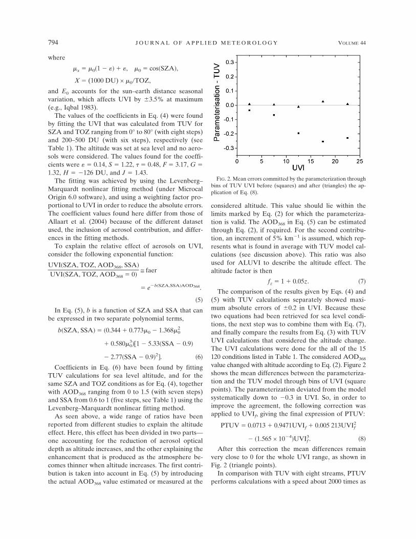
The comparison of the results given by Eqs. (4) and(5) with TUV calculations separately showed maxi-mum absolute errors of �0.2 in UVI. Because thesetwo equations had been retrieved for sea level condi-tions, the next step was to combine them with Eq. (7),and finally compare the results from Eq. (3) with TUVUVI calculations that considered the altitude change.The UVI calculations were done for the all of the 15120 conditions listed in Table 1. The considered AOD368

value changed with altitude according to Eq. (2). Figure 2shows the mean differences between the parameteriza-tion and the TUV model through bins of UVI (squarepoints). The parameterization deviated from the modelsystematically down to �0.3 in UVI. So, in order toimprove the agreement, the following correction wasapplied to UVIf, giving the final expression of PTUV:

PTUV � 0.0713 � 0.9471UVIf � 0.005 213UVIf2

� �1.565 × 10�4�UVIf3. �8�

After this correction the mean differences remainvery close to 0 for the whole UVI range, as shown inFig. 2 (triangle points).

In comparison with TUV with eight streams, PTUVperforms calculations with a speed about 2000 times as

FIG. 2. Mean errors committed by the parameterization throughbins of TUV UVI before (squares) and after (triangles) the ap-plication of Eq. (8).


fast. In comparison with the two-streams code, thePTUV is about 50 times as fast.

d. Model versus parameterization

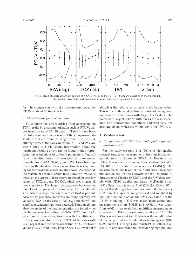
To estimate the errors arising from approximatingTUV results by a parameterization such as PTUV, val-ues from the same 15 120 cases in Table 1 have beencarefully compared. As a result of the comparison, ab-solute errors are found to range from �0.26 to 0.34,although 88% of the cases are within �0.1, and 99% arewithin �0.2 in UVI. Useful information about themaximum absolute errors can be found in their repre-sentation as functions of different parameters. Figure 3shows the distribution of averaged absolute errorsthrough bins of SZA, TOZ, z, and UVI. Error bars rep-resenting the standard deviation and two curves account-ing for the maximum errors are also shown. As expected,the maximum absolute errors take place for low SZA;however, the largest of these errors are found for very lowvalues of TOZ, around 200 DU, which are, in general,rare conditions. The largest discrepancies between themodel and the parameterization occur for low-altitudesites, where a large fraction of aerosol load is present.Also the largest absolute errors are found for very lowvalues of SSA. In the case of AOD368 (not shown), nosignificant tendency has been detected. Thus, maximumabsolute errors of the parameterization are found whencombining very low values of SZA, TOZ, and SSA,which are extreme cases, together with low altitude.

Concerning relative errors, in 95% of the cases withUVI larger than 2 the errors are within �3%. For lowervalues of UVI (and, thus, larger SZA, i.e., lower solar

altitudes) the relative errors take much larger values.This is due to the model-fitting criterion of giving moreimportance to the points with larger UVI values. Thepoints with largest relative differences are also associ-ated with noncommon conditions and with very lowabsolute errors, which are within �0.19 for UVI � 2.

3. Validation test

a. Comparison with UVI from high-quality spectralmeasurements

For this study we took 1 yr (2001) of high-qualityspectral irradiance measurements from an instrumentmanufactured in house at NIWA (McKenzie et al.1992). It was sited in Lauder, New Zealand [45.04°S,169.684°E, 370 m above mean sea level (MSL)]. Themeasurements are taken at the Southern Hemispheremidlatitude site for the Network for the Detection ofStratospheric Change (NDSC), and the UV data com-ply with NDSC quality standards (McKenzie et al.1997). Spectra are taken at 5° of SZA (for SZA � 95°),except that during 2 h around noontime the frequencyis 15 min. The spectra are processed and weighted bythe CIE function to obtain the UV index value. For thePTUV modeling, TOZ was taken from assimilatedmeasurements from TOMS and AOD368 was takenfrom AOD412 retrievals from multifilter measurementsconverted to 368 nm, considering an alpha of 1.4. TheSSA was set constant to 0.9, which is the middle valueof the range that is considered as being typical (0.8–0.999) in the UV range (Madronich 1993; Petters et al.2003). In any case, when not considering high-polluted

FIG. 3. Mean absolute errors as function of SZA, TOZ, z, and TUV UVI. Standard deviation is shown throughthe vertical error bars, and maximum absolute errors are represented in lines.


sites, the effect of slight differences in SSA values is low(Petters et al. 2003).

Only entirely clear days were selected for the com-parison, although we were forced to remove some halfdays because of the lack of AOD measurements. In thisway, 11% of the initial dataset was finally considered,which is a total of 979 records, with 11 summer days, 21autumn days, 18 winter days, and 7 spring days.

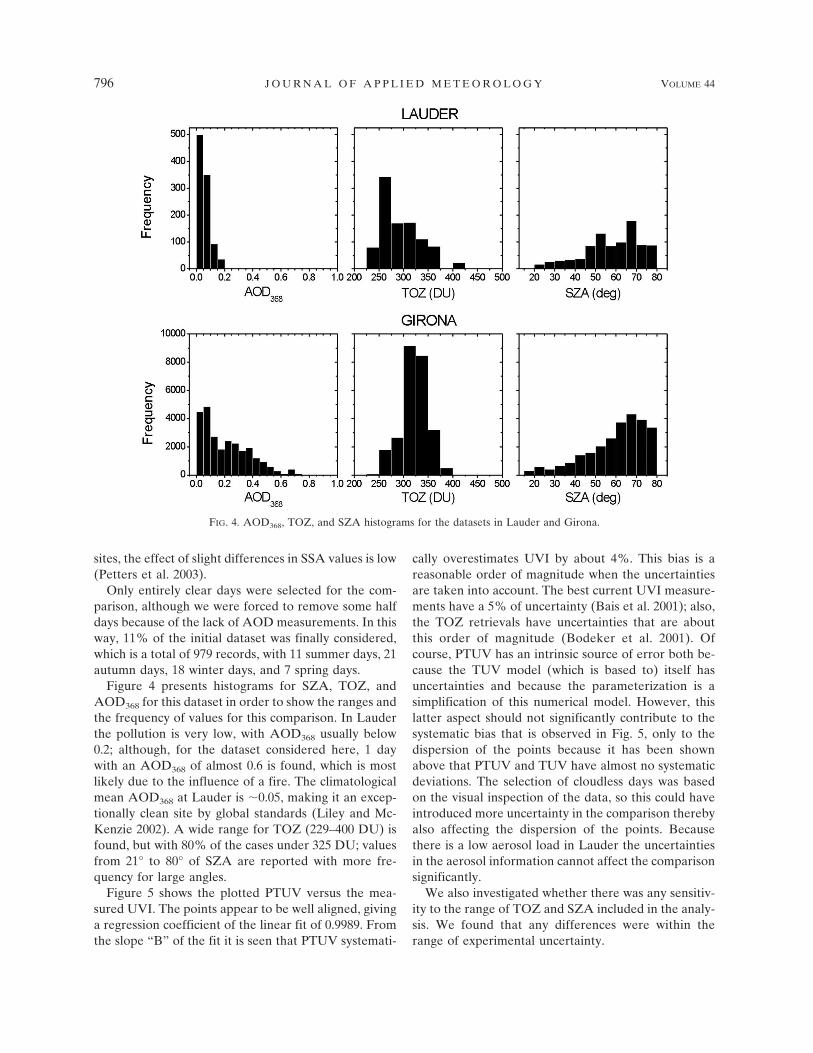
Figure 4 presents histograms for SZA, TOZ, andAOD368 for this dataset in order to show the ranges andthe frequency of values for this comparison. In Lauderthe pollution is very low, with AOD368 usually below0.2; although, for the dataset considered here, 1 daywith an AOD368 of almost 0.6 is found, which is mostlikely due to the influence of a fire. The climatologicalmean AOD368 at Lauder is �0.05, making it an excep-tionally clean site by global standards (Liley and Mc-Kenzie 2002). A wide range for TOZ (229–400 DU) isfound, but with 80% of the cases under 325 DU; valuesfrom 21° to 80° of SZA are reported with more fre-quency for large angles.

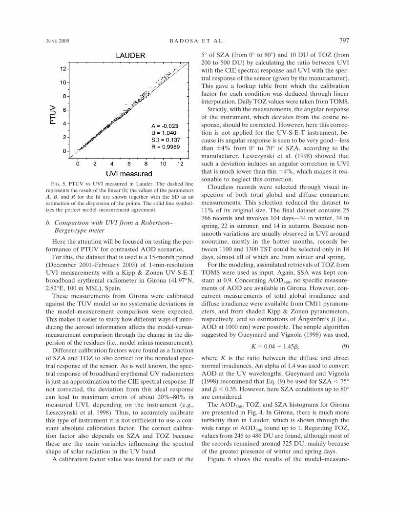
Figure 5 shows the plotted PTUV versus the mea-sured UVI. The points appear to be well aligned, givinga regression coefficient of the linear fit of 0.9989. Fromthe slope “B” of the fit it is seen that PTUV systemati-

cally overestimates UVI by about 4%. This bias is areasonable order of magnitude when the uncertaintiesare taken into account. The best current UVI measure-ments have a 5% of uncertainty (Bais et al. 2001); also,the TOZ retrievals have uncertainties that are aboutthis order of magnitude (Bodeker et al. 2001). Ofcourse, PTUV has an intrinsic source of error both be-cause the TUV model (which is based to) itself hasuncertainties and because the parameterization is asimplification of this numerical model. However, thislatter aspect should not significantly contribute to thesystematic bias that is observed in Fig. 5, only to thedispersion of the points because it has been shownabove that PTUV and TUV have almost no systematicdeviations. The selection of cloudless days was basedon the visual inspection of the data, so this could haveintroduced more uncertainty in the comparison therebyalso affecting the dispersion of the points. Becausethere is a low aerosol load in Lauder the uncertaintiesin the aerosol information cannot affect the comparisonsignificantly.

We also investigated whether there was any sensitiv-ity to the range of TOZ and SZA included in the analy-sis. We found that any differences were within therange of experimental uncertainty.

FIG. 4. AOD368, TOZ, and SZA histograms for the datasets in Lauder and Girona.


b. Comparison with UVI from a Robertson–Berger-type meter

Here the attention will be focused on testing the per-formance of PTUV for contrasted AOD scenarios.

For this, the dataset that is used is a 15-month period(December 2001–February 2003) of 1-min-resolutionUVI measurements with a Kipp & Zonen UV-S-E-Tbroadband erythemal radiometer in Girona (41.97°N,2.82°E, 100 m MSL), Spain.

These measurements from Girona were calibratedagainst the TUV model so no systematic deviations inthe model–measurement comparison were expected.This makes it easier to study how different ways of intro-ducing the aerosol information affects the model-versus-measurement comparison through the change in the dis-persion of the residues (i.e., model minus measurement).

Different calibration factors were found as a functionof SZA and TOZ to also correct for the nonideal spec-tral response of the sensor. As is well known, the spec-tral response of broadband erythemal UV radiometersis just an approximation to the CIE spectral response. Ifnot corrected, the deviation from this ideal responsecan lead to maximum errors of about 20%–80% inmeasured UVI, depending on the instrument (e.g.,Leszczynski et al. 1998). Thus, to accurately calibratethis type of instrument it is not sufficient to use a con-stant absolute calibration factor. The correct calibra-tion factor also depends on SZA and TOZ becausethese are the main variables influencing the spectralshape of solar radiation in the UV band.

A calibration factor value was found for each of the

5° of SZA (from 0° to 80°) and 10 DU of TOZ (from200 to 500 DU) by calculating the ratio between UVIwith the CIE spectral response and UVI with the spec-tral response of the sensor (given by the manufacturer).This gave a lookup table from which the calibrationfactor for each condition was deduced through linearinterpolation. Daily TOZ values were taken from TOMS.

Strictly, with the measurements, the angular responseof the instrument, which deviates from the cosine re-sponse, should be corrected. However, here this correc-tion is not applied for the UV-S-E-T instrument, be-cause its angular response is seen to be very good—lessthan �4% from 0° to 70° of SZA, according to themanufacturer. Leszczynski et al. (1998) showed thatsuch a deviation induces an angular correction in UVIthat is much lower than this �4%, which makes it rea-sonable to neglect this correction.

Cloudless records were selected through visual in-spection of both total global and diffuse concurrentmeasurements. This selection reduced the dataset to11% of its original size. The final dataset contains 25766 records and involves 104 days—34 in winter, 34 inspring, 22 in summer, and 14 in autumn. Because non-smooth variations are usually observed in UVI aroundnoontime, mostly in the hotter months, records be-tween 1100 and 1300 TST could be selected only in 18days, almost all of which are from winter and spring.

For the modeling, assimilated retrievals of TOZ fromTOMS were used as input. Again, SSA was kept con-stant at 0.9. Concerning AOD368, no specific measure-ments of AOD are available in Girona. However, con-current measurements of total global irradiance anddiffuse irradiance were available from CM11 pyranom-eters, and from shaded Kipp & Zonen pyranometers,respectively, and so estimations of Ångström’s � (i.e.,AOD at 1000 nm) were possible. The simple algorithmsuggested by Gueymard and Vignola (1998) was used,

K � 0.04 � 1.45�, �9�

where K is the ratio between the diffuse and directnormal irradiances. An alpha of 1.4 was used to convertAOD at the UV wavelengths. Gueymard and Vignola(1998) recommend that Eq. (9) be used for SZA � 75°and � � 0.35. However, here SZA conditions up to 80°are considered.

The AOD368, TOZ, and SZA histograms for Gironaare presented in Fig. 4. In Girona, there is much moreturbidity than in Lauder, which is shown through thewide range of AOD368 found up to 1. Regarding TOZ,values from 246 to 486 DU are found, although most ofthe records remained around 325 DU, mainly becauseof the greater presence of winter and spring days.

Figure 6 shows the results of the model–measure-

FIG. 5. PTUV vs UVI measured in Lauder. The dashed linerepresents the result of the linear fit; the values of the parametersA, B, and R for the fit are shown together with the SD as anestimation of the dispersion of the points. The solid line symbol-izes the perfect model–measurement agreement.


ment comparison through the model-versus-measure-ment and residues-versus-SZA plots. Apart from theresults considering PTUV with the aerosol informationdescribed above, there are two additional comparisonsusing different types of modeling that consider twoother ways of taking into account (implicitly and ex-plicitly) the aerosol contribution.

On the one hand, the results with UVI calculatedwith ALUVI are also shown. This formula considersthe SZA, TOZ, E0, and a 5% km�1 altitude effect asinput information and is a result of fitting UVI fromBrewer spectrophotometer measurements taken in DeBilt (Netherlands) and Paramaribo (Surinam). Thus,ALUVI has implicit aerosol information. On the otherhand, PTUV is used with climatic information ofAOD368 as input. Monthly typical values of Ångström’s� in Girona are considered from González et al. (2001)based on an algorithm that is more rigorous (Gueymard1998) than the one in Eq. (9) that was applied to 4 yr ofbroadband total and diffuse measurements. Despite thelimited period, these typical values will be consideredas climatic hereinafter. An alpha value of 1.4 is usedthen to convert AOD to 368 nm. This annual variationof AOD368 is shown in Fig. 7.

As shown in Fig. 6, for the three cases the model-versus-measurement plots (Figs. 6a1, 6b1, 6c1) showexcellent correlations, with R always larger than 0.996.For Fig. 6a1, which corresponds to the comparison us-ing ALUVI, a good slope is found, with B � 0.991. InFig. 6b1, for which PTUV with climatic AOD is used, alower slope is found, with B � 0.976.

FIG. 6. 1) UVI modeled-vs-measured and 2) the residues vs SZA plots for with the dataset from Girona and threedifferent ways of modeling—(a) ALUVI; (b) PTUV with AOD climatic from González et al. (2001); (c) PTUVwith the actual AOD conditions from Eq. (9). Dashed lines and solid lines are represented in model-vs-measurement plots accounting for the linear fit and perfect agreement lines, respectively. The linear fit statisticalparameters A, B, SD, and R are also shown.

FIG. 7. Annual variation of SZA (solid line) in degrees, TOZ(dotted line) in DU, and AOD368 (dashed line) for Girona.


The linear fit for Fig. 6c1 gives B very close to 1 (B �1.003), which is logical, given the way the measure-ments were calibrated. Notice that PTUV tends to un-derestimate the UVI measurements by about 2.2%because of the different aerosol information that is con-sidered. The most remarkable aspect is the clear differ-ences that are observed in the dispersion of the points,which are mathematically expressed through the stan-dard deviation (SD). The largest dispersion is found forALUVI (SD � 0.167) because of its implicit and place-based treatment of aerosols. When climatic values forAOD are introduced to PTUV, a lower SD value isfound (SD � 0.131). The lowest dispersion is foundwhen more aerosol information is considered in themodel, that is, in the Fig. 6c1, where SD � 0.097. Thisimplies a reduction in SD of 27% with regard to the SDfor PTUV with climatic AOD.

These differences in the dispersion are also clearlyevident in the residues-versus-SZA plots (Figs. 6a2,6b2, 6c2). For the comparison with ALUVI, the follow-ing widest range of residues is found: �0.95 � 0.60 inUVI. In Fig. 6b2, from the comparison using PTUVwith climatic AOD, a slightly narrower range is foundof �0.90 � 0.42 in UVI. The residues for PTUV withconcurrent AOD368 from Eq. (9) (Fig. 6c2) take valueswithin a limited range in UVI of �0.37. Thus, a clearrelation appears between SD and the residues range; sothe larger the SD the larger the residue range.

These analyses show that the PTUV model is able toexplain different (but not extreme) AOD situations,giving a good model–measurement agreement. More-over, from Fig. 6 it is apparent that considering concur-rent information for AOD into the model gives muchbetter results than taking into account climatic valuesor implicit contributions. Slightly better results in thedispersion of the points are found when climatic aerosolinformation from the working site is explicitly intro-duced to PTUV, as compared with ALUVI, which im-plicitly considers aerosol information from a differentsite. In spite of this, a better model-versus-measure-ment agreement (i.e., a value of B closer to 1) is foundfor ALUVI than for PTUV with climatic AOD.

The reason why PTUV with climatic AOD andALUVI give similar results for Girona is because theaerosol characteristics for this site are similar to thosein the measurements that are used to retrieve ALUVI.The latter algorithm, when applied to the dataset fromLauder (section 3a), gives UVI values that are 6%lower than PTUV (with both climatic AOD estimationsand the AOD actual measurements that are available),because the aerosol contribution that is implicitly ac-counted for by ALUVI is overestimated.

4. Seasonal UVI maps

a. Climatic annual variation of UVI

To know the typical UVI values for Catalonia it isinteresting to see the seasonal variation of some of thevariables that affect UVI most, that is, SZA, TOZ, andAOD. For this analysis, Girona has been chosen be-cause for this site there are some data that are availableabout typical turbidity on a monthly basis (González etal. 2001), as discussed above. TOZ is calculated throughmoving averages of �5 days from 25 yr (1979–2003) ofEarth Probe TOMS assimilated measurements. Be-cause these measurements have a latitude � longituderesolution of 1° � 1.25°, Catalonia is completely coveredwith seven cells (see Fig. 1). Girona is very close to theborder between cell 3 and 6, and so the TOZ for this sitehas been calculated as the mean value of these two cells.

Figure 7 shows the annual change of noontime SZA,TOZ, and AOD368. Maximum TOZ values are detectedin April, and minimum values are at the end of Octoberand beginning of November; the range is 284–370 DU.Monthly climatic values of AOD368 range from 0.04 (inJanuary) to 0.47 (in July). The shape of the curve showsthat there are more aerosols during spring than in au-tumn. The range of noontime SZA for the considereddataset is from 18.5° to 65.4°.

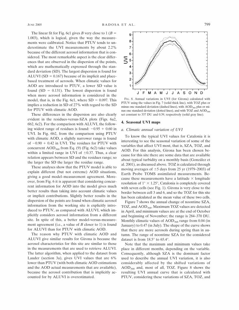
Note that the maximum and minimum values takeplace in different months, depending on the variable.Consequently, although SZA is the dominant factorused to describe the annual UVI variation, it is alsoconsiderably affected by the shifted variations ofAOD368 and, most of all, TOZ. Figure 8 shows theresulting UVI annual curve that is calculated withPTUV, considering these variations of SZA, TOZ, and

FIG. 8. Annual variations in UVI (for Girona) calculated withPTUV using the values in Fig. 7 (solid thick line), with TOZ plus orminus one standard deviation (dashed lines), with AOD368 plus or mi-nus one standard deviation (dotted lines), and with TOZ and AOD368

set constant to 337 DU and 0.39, respectively (solid gray line).


AOD368 (thick line). The UVI curve that is calculatedwith the summer solstice mean TOZ (337 DU) andAOD368 (0.39) values (solid gray line) is also plotted.Differences in the shapes of the curves are clear. The“realistic” line is asymmetric with respect to the sum-mer solstice, with UVI values that are about 1 unitlarger at the autumn equinox than at the spring equinoxand some oscillations, which are mainly caused by theTOZ annual and day-to-day variations. Moreover, themaximum UVI of the curve, which is around 8, is de-tected during all of June and July and not only aroundthe summer solstice, which is an important aspect totake into account for UV damage prevention purposes.This fact is produced by the reduction in TOZ in sum-mer that partly compensates for the effect of the in-crease of the noontime SZA.

Figure 8 also shows the UVI curves for TOZ andAOD368 from Fig. 7 plus and minus one standard de-viation. The std devs of TOZ are around 34–44 DU inwinter, 19–41 DU in spring, 12–20 DU in summer, and16–31 DU in autumn. This leads to much larger day-to-day variability of UVI in the first two seasons thanfor the latter two, which is clearly seen in Fig. 8 (dashedcurves). Concerning AOD368, the std dev is around 0.17in summer and is much lower, around 0.05, in winter.This aerosol variability induces variability in UVI (dot-ted curves) that is comparable with the TOZ-inducedvariability near summer but is much lower for the restof the year. This gives more evidence that it is impor-tant to know the aerosol (or turbidity) properties tocharacterize UVI accurately, particularly in summer.

While the annual UVI considering the climatologicalmean values of TOZ and AOD368 reaches a maximumof 8 units, when introducing TOZ and AOD368 minustheir std devs into PTUV, a June–July UVI of 9.3 isreached (the corresponding curve is not shown here),which is 16% larger.

All of these considerations show the complexity ofUVI values that are expected. For the construction oftypical UVI maps in Catalonia, climatological meanvalues of TOZ and AOD368 will be used, but the com-ments above have to be taken into account.

b. Construction of seasonal UVI maps

Four maps are presented, corresponding to the sol-stices and equinoxes at noon, in order to see the sea-sonal differences (see Fig. 9). A resolution of 1 km � 1km is taken, which involves 268 � 278 nodes.

The values of TOZ have been found also from mov-ing averages of �5 days of 25 yr and averaging togetherthe seven values that TOMS gives for all of the regionof Catalonia each day (see Fig. 1). In this way, for eachday one value of TOZ is taken to represent all of the

territory. Badosa (2002) showed that the TOZ from theseven cells of TOMS were highly correlated andshowed no significant systematic differences. Conse-quently, it is a good approximation to assign only oneTOZ value for Catalonia, although this simplification isless suitable in spring and winter when the TOZ vari-ability is at a maximum.

Because we do not have any climatic informationabout aerosols for Catalonia, the monthly values of Fig.7 have been considered to represent all of the territory.Although this situation is far from ideal, we note thatthis annual turbidity evolution is very similar to whatother authors found from analyses for Mediterraneansites, such as Barcelona and Valencia (Lorente 1978;Pinazo et al. 1995; Pedrós et al. 1999). Equation (2) isused to extrapolate AOD368 for different altitudes.

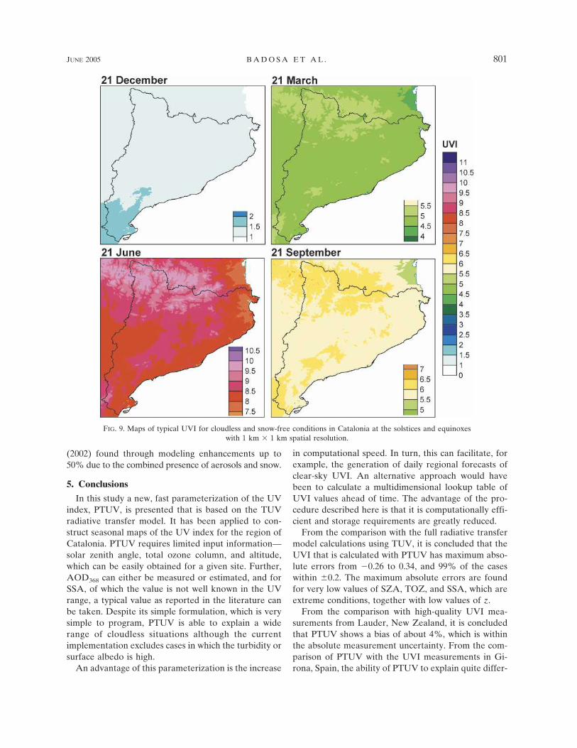
In Fig. 9 much larger UVI values for 21 June (UVI upto 10.5) than for 21 December (UVI up to 2) are re-ported, as expected. It is also seen that UVI for 21September and 21 March is around 6.5 and 5.5, respec-tively, showing about 1 point in UVI of difference, asalso appeared in the above analysis for Girona.

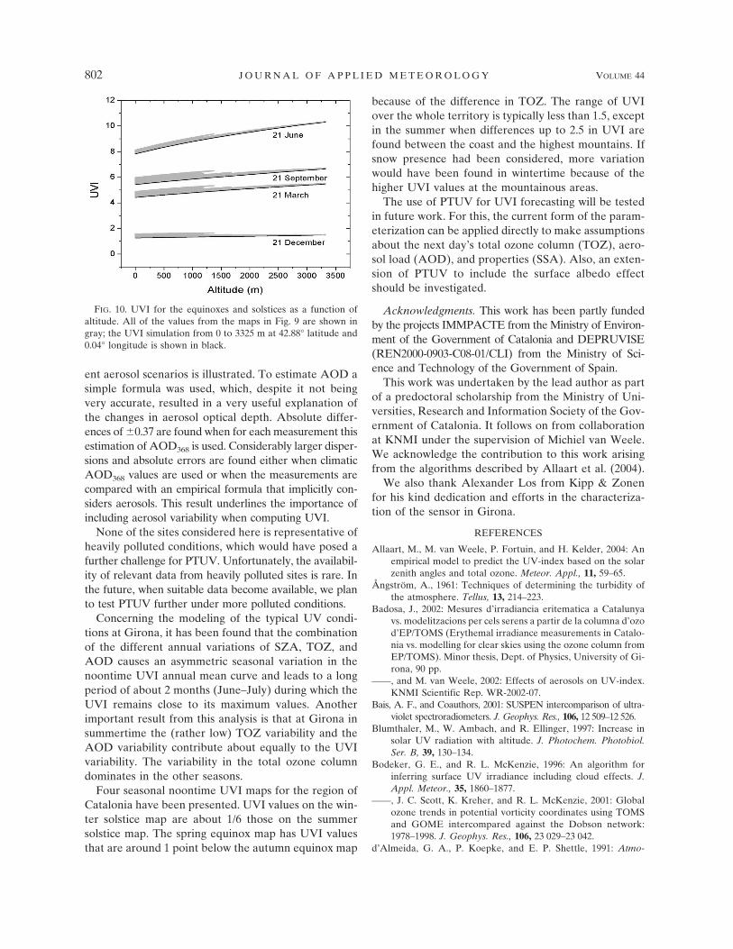
Figure 10 shows (in gray) all of the UVI values foreach map, plotted as a function of altitude. The par-ticular case of UVI that is simulated over a range ofaltitudes from 0 to 3325 m at 42.88°N and 0.04°E(northeast corner of the maps) is shown through theblack lines. Because Catalonia is a relatively small ter-ritory, the latitudinal effect is rather weak. This effectappears in Fig. 10 as the vertical dispersion of the points,which is larger for the equinoxes than for the solstices.

The altitude effect is less obvious for the nonsummermaps. Even the relative changes with altitude aresmaller in winter than in summer because of the re-duced aerosol loading in the boundary layer in winter(relative changes are up to 17% in winter and up to 30%in summer, as calculated from Fig. 10). For the autumn,winter, and spring maps, a maximum difference less than1.5 in UVI is found for the whole territory. In summerthe altitude effect strongly appears with differences upto 2.5 between the coast and the highest mountains.This shows, first, the need to take into account the al-titude effect in Catalonia and, second, that high andharmful UV levels occur in the mountain regions.

Situations with large albedo, such as snow-coveredsurfaces, are not considered here. It is known that UVIin these situations is considerably enhanced. For ex-ample, Renaud et al. (2000) reported increments inUVI of 15%–25% due to the multiple ground–atmosphere reflections under the cloudless sky andsnow-covered surface conditions. McKenzie et al.(1998) showed increases of 28% for clear skies, andincreases exceeding 50% under cloudy skies. Badosa


(2002) found through modeling enhancements up to50% due to the combined presence of aerosols and snow.

5. Conclusions

In this study a new, fast parameterization of the UVindex, PTUV, is presented that is based on the TUVradiative transfer model. It has been applied to con-struct seasonal maps of the UV index for the region ofCatalonia. PTUV requires limited input information—solar zenith angle, total ozone column, and altitude,which can be easily obtained for a given site. Further,AOD368 can either be measured or estimated, and forSSA, of which the value is not well known in the UVrange, a typical value as reported in the literature canbe taken. Despite its simple formulation, which is verysimple to program, PTUV is able to explain a widerange of cloudless situations although the currentimplementation excludes cases in which the turbidity orsurface albedo is high.

An advantage of this parameterization is the increase

in computational speed. In turn, this can facilitate, forexample, the generation of daily regional forecasts ofclear-sky UVI. An alternative approach would havebeen to calculate a multidimensional lookup table ofUVI values ahead of time. The advantage of the pro-cedure described here is that it is computationally effi-cient and storage requirements are greatly reduced.

From the comparison with the full radiative transfermodel calculations using TUV, it is concluded that theUVI that is calculated with PTUV has maximum abso-lute errors from �0.26 to 0.34, and 99% of the caseswithin �0.2. The maximum absolute errors are foundfor very low values of SZA, TOZ, and SSA, which areextreme conditions, together with low values of z.

From the comparison with high-quality UVI mea-surements from Lauder, New Zealand, it is concludedthat PTUV shows a bias of about 4%, which is withinthe absolute measurement uncertainty. From the com-parison of PTUV with the UVI measurements in Gi-rona, Spain, the ability of PTUV to explain quite differ-

FIG. 9. Maps of typical UVI for cloudless and snow-free conditions in Catalonia at the solstices and equinoxeswith 1 km � 1 km spatial resolution.


Fig 9 live 4/C

ent aerosol scenarios is illustrated. To estimate AOD asimple formula was used, which, despite it not beingvery accurate, resulted in a very useful explanation ofthe changes in aerosol optical depth. Absolute differ-ences of �0.37 are found when for each measurement thisestimation of AOD368 is used. Considerably larger disper-sions and absolute errors are found either when climaticAOD368 values are used or when the measurements arecompared with an empirical formula that implicitly con-siders aerosols. This result underlines the importance ofincluding aerosol variability when computing UVI.

None of the sites considered here is representative ofheavily polluted conditions, which would have posed afurther challenge for PTUV. Unfortunately, the availabil-ity of relevant data from heavily polluted sites is rare. Inthe future, when suitable data become available, we planto test PTUV further under more polluted conditions.

Concerning the modeling of the typical UV condi-tions at Girona, it has been found that the combinationof the different annual variations of SZA, TOZ, andAOD causes an asymmetric seasonal variation in thenoontime UVI annual mean curve and leads to a longperiod of about 2 months (June–July) during which theUVI remains close to its maximum values. Anotherimportant result from this analysis is that at Girona insummertime the (rather low) TOZ variability and theAOD variability contribute about equally to the UVIvariability. The variability in the total ozone columndominates in the other seasons.

Four seasonal noontime UVI maps for the region ofCatalonia have been presented. UVI values on the win-ter solstice map are about 1/6 those on the summersolstice map. The spring equinox map has UVI valuesthat are around 1 point below the autumn equinox map

because of the difference in TOZ. The range of UVIover the whole territory is typically less than 1.5, exceptin the summer when differences up to 2.5 in UVI arefound between the coast and the highest mountains. Ifsnow presence had been considered, more variationwould have been found in wintertime because of thehigher UVI values at the mountainous areas.

The use of PTUV for UVI forecasting will be testedin future work. For this, the current form of the param-eterization can be applied directly to make assumptionsabout the next day’s total ozone column (TOZ), aero-sol load (AOD), and properties (SSA). Also, an exten-sion of PTUV to include the surface albedo effectshould be investigated.

Acknowledgments. This work has been partly fundedby the projects IMMPACTE from the Ministry of Environ-ment of the Government of Catalonia and DEPRUVISE(REN2000-0903-C08-01/CLI) from the Ministry of Sci-ence and Technology of the Government of Spain.

This work was undertaken by the lead author as partof a predoctoral scholarship from the Ministry of Uni-versities, Research and Information Society of the Gov-ernment of Catalonia. It follows on from collaborationat KNMI under the supervision of Michiel van Weele.We acknowledge the contribution to this work arisingfrom the algorithms described by Allaart et al. (2004).

We also thank Alexander Los from Kipp & Zonenfor his kind dedication and efforts in the characteriza-tion of the sensor in Girona.

REFERENCES

Allaart, M., M. van Weele, P. Fortuin, and H. Kelder, 2004: Anempirical model to predict the UV-index based on the solarzenith angles and total ozone. Meteor. Appl., 11, 59–65.

Ångström, A., 1961: Techniques of determining the turbidity ofthe atmosphere. Tellus, 13, 214–223.

Badosa, J., 2002: Mesures d’irradiancia eritematica a Catalunyavs. modelitzacions per cels serens a partir de la columna d’ozod’EP/TOMS (Erythemal irradiance measurements in Catalo-nia vs. modelling for clear skies using the ozone column fromEP/TOMS). Minor thesis, Dept. of Physics, University of Gi-rona, 90 pp.

——, and M. van Weele, 2002: Effects of aerosols on UV-index.KNMI Scientific Rep. WR-2002-07.

Bais, A. F., and Coauthors, 2001: SUSPEN intercomparison of ultra-violet spectroradiometers. J. Geophys. Res., 106, 12 509–12 526.

Blumthaler, M., W. Ambach, and R. Ellinger, 1997: Increase insolar UV radiation with altitude. J. Photochem. Photobiol.Ser. B, 39, 130–134.

Bodeker, G. E., and R. L. McKenzie, 1996: An algorithm forinferring surface UV irradiance including cloud effects. J.Appl. Meteor., 35, 1860–1877.

——, J. C. Scott, K. Kreher, and R. L. McKenzie, 2001: Globalozone trends in potential vorticity coordinates using TOMSand GOME intercompared against the Dobson network:1978–1998. J. Geophys. Res., 106, 23 029–23 042.

d’Almeida, G. A., P. Koepke, and E. P. Shettle, 1991: Atmo-

FIG. 10. UVI for the equinoxes and solstices as a function ofaltitude. All of the values from the maps in Fig. 9 are shown ingray; the UVI simulation from 0 to 3325 m at 42.88° latitude and0.04° longitude is shown in black.


spheric Aerosols: Global Climatology and Radiative Charac-teristics. A. Deepak Publishing, 561 pp.

Elterman, L., 1968: UV, visible, and IR attenuation for altitudesto 50 km. Air Force Cambridge Research Laboratory Envi-ronmental Research Paper 285, AFCRL-68-0153, 49 pp.

Fioletov, V. E., J. B. Kerr, L. J. B. McArthur, D. I. Wardle, andT. W. Mathews, 2003: Estimating UV index climatology overCanada. J. Appl. Meteor., 42, 417–433.

González, J.-A., J. Mejías, and J. Calbó, 2001: Aplicación demétodos basados en medidas radiativas de banda ancha a ladeterminación de la turbidez atmosférica en Girona (Appli-cation of methods based on broadband radiative measure-ments and the atmospheric turbidity determination in Gi-rona). El tiempo del clima (Weather and Climate), A. J. Pérez-Cueva et al., Eds., Publicaciones de la Asociación Españolade Climatología, 467–475.

Gueymard, C. A., 1998: Turbidity determination from broadbandirradiance measurements: A detailed multicoefficient ap-proach. J. Appl. Meteor., 37, 414–435.

——, and F. Vignola, 1998: Determination of atmospheric turbid-ity from the diffuse-beam broadband irradiance ratio. Sol.Energy, 63, 135–146.

Herman, J. R., R. L. McKenzie, S. B. Diaz, J. B. Kerr, S. Mad-ronich, and G. Seckmeyer, 1999: Ultraviolet radiation at theEarth’s surface. UNEP/WMO Scientific Assessment of theOzone Layer: 1998, D. L. Albritton et al., Eds., Global OzoneResearch and Monitoring Project Rep. 44, 9.1–9.46

Iqbal, M., 1983: An Introduction to Solar Radiation. Academic, 390 pp.Jacobson, M. Z., 1998: Isolating the causes and effects of large

ultraviolet reductions in Los Angeles. J. Aerosol Sci., 29(Suppl.), S655–S656.

——, 1999: Isolating nitrated and aromatic aerosols and nitratedaromatic gases as sources of ultraviolet light absorption. J.Geophys. Res., 104, 3527–3542.

Lenoble, J., 1993: Atmospheric Radiative Transfer. A. DeepakPublishing, 532 pp.

Leszczynski, K., K. Jokela, L. Ylianttila, R. Visuri, and M.Blumthaler, 1998: Erythemally weighted radiometers in solarUV monitoring: Results from the WMO/STUK intercom-parison. Photochem. Photobiol., 67, 212–221.

Liley, J. B., and R. L. McKenzie, 2002: Air clarity implications forsolar radiation at the surface. Proc. 16th Int. Clean Air and Envi-ronment Conf., Christchurch, New Zealand, CASANZ, 502–505.

Lorente, J., 1978: Contribución al estudio de la turbiedad atmos-férica en Barcelona (Contribution to the study of atmo-spheric turbidity in Barcelona). Rev. Geofis., 2, 155–167.

Madronich, S., 1993: UV radiation in the natural and perturbedatmosphere. Environmental Effects of UV (Ultraviolet) Ra-diation, M. Tevini, Ed., Lewis Publisher, 17–69.

——, R. L. McKenzie, M. M. Caldwell, and L. O. Björn, 1994:Changes in ultraviolet radiation reaching the earth’s surface.Environmental Effects of Ozone Depletion: 1994 Assess-ment, United Nations Environment Programme, 1–22.

McClatchey, R. A., R. W. Fenn, J. E. A. Selby, F. E. Volz, andJ. S. Garing, 1972: Optical properties of the atmosphere. 3ded. AFCRL Environmental Research Paper 411, 108 pp.

McKenzie, R. L., P. V. Johnston, M. Kotkamp, A. Bittar, and J. D.Hamlin, 1992: Solar ultraviolet spectroradiometry in NewZealand: Instrumentation and sample results from 1990.Appl. Opt., 31, 6501–6509.

——, ——, and G. Seckmeyer, 1997: UV spectro-radiometry inthe network for the detection of stratospheric change(NDSC). Solar Ultraviolet Radiation: Modelling, Measure-

ments, and Effects, C. S. Zerefos and A. F. Bais, Eds., NATOASI Series, Vol. 1.52, Springer-Verlag, 279–287.

——, K. J. Paulin, and S. Madronich, 1998: Effects of snow coveron UV radiation and surface albedo: A case study. J. Geo-phys. Res., 103, 28 785–28 792.

——, P. V. Johnston, D. Smale, B. Bodhaine, and S. Madronich,2001a: Altitude effects on UV spectral irradiance deducedfrom measurements at Lauder, New Zealand and at MaunaLoa Observatory, Hawaii. J. Geophys. Res., 106, 22 845–22 860.

——, G. Seckmeyer, A. Bais, and S. Madronich, 2001b: Satelliteretrievals of erythemal UV dose compared with ground-based measurements at northern and southern mid-latitudes.J. Geophys. Res., 106, 24 051–24 062.

McKinlay, A. F., and B. L. Diffey, 1987: A reference action spec-trum for ultraviolet induced erythema in human skin. HumanExposure to Ultraviolet Radiation: Risks and Regulations, W.R. Passchier and B. M. F. Bosnajakovich, Eds., Elsevier, 83–87.

Pedrós, R., M. P. Utrillas, J. A. Martínez-Lozano, and F. Tena,1999: Values of broad band turbidity coefficients in a Medi-terranean coastal site. Sol. Light, 66, 11–20.

Petters, J. L., V. K. Saxena, J. R. Slusser, B. N. Wenny, and S. Mad-ronich, 2003: Aerosol single scattering albedo retrieved frommeasurements of surface UV irradiance and a radiative transfermodel. J. Geophys. Res., 108, 4288, doi:10.1029/2002JD002360.

Pinazo, J. M., J. Cañada, and J. V. Boscá, 1995: A new methoddetermine Ångstrom’s turbidity coefficient: Its applicationfor Valencia. Sol. Energy, 54, 219–226.

Radiation Commission of IAMAP, 1986: A preliminary cloudlessstandard atmosphere for radiation computation. Rep. WCP-112, WMO/TD 24, 53 pp.

Renaud, A., J. Staehelin, C. Fröhlich, R. Philipona, and A. He-imo, 2000: Influence of snow and clouds on erythemal UVradiation: Analysis of Swiss measurements and comparisonwith models. J. Geophys. Res., 105, 4961–4969.

Reuder, J., and H. Schwander, 1999: Aerosol effects on UV radia-tion in nonurban regions. J. Geophys. Res., 104, 4065–4077.

Schmalwieser, A. W., and G. Schauberger, 2001: A monitoring net-work for erythemally-effective solar ultraviolet radiation inAustria: Determination of the measuring sites and visualisationof the spatial distribution. Theor. Appl. Climatol., 69, 221–229.

——, and Coauthors, 2002: Worldwide forecast of the biologically effec-tive UV radiation: UV index and daily dose. Ultraviolet Ground-and Space-based Measurements, Models, and Effects. J. R. Slusser,J. R. Herman, and W. Gao, Eds., International Society for Op-tical Engineering (SPIE Proceedings Vol. 4482), 259–264.

Schmucki, D., and R. Philipona, 2001: UV radiation in the Alps: Alti-tude effect. Extended Abstracts, EGS XXVI General Assembly,Nice, France, European Geophysical Society, Vol. 3, CD-ROM.

Vanicek, K., T. Frei, Z. Litynska, and A. Schmalwieser, 2000: UVindex for the public. Working Group 4 of the COST-713Action “UVB Forecasting.” [Available online at http://www.lamma.rete.toscana.it/uvweb/.]

Verdebout, J., 2000: A method to generate surface UV radiationmaps over Europe using GOME, Meteosat, and ancillarydata. J. Geophys. Res., 105, 5049–5058.

Weihs, P., and Coauthors, 2002: Effective surface albedo due tosnow cover of the surrounding area. Ultraviolet Ground- andSpace-based Measurements, Models, and Effects. J. R. Slusser,J. R. Herman, and W. Gao, Eds., International Society for Op-tical Engineering (SPIE Proceedings Vol. 4482), 152–159.

Zaratti, F., R. N. Forno, J. Garcia Fuentes, and M. F. Andrade,2003: Erythemally weighted UV variations at two high-alti-tude locations. J. Geophys. Res., 108, 4263–4268.


Using a Parameterization of a Radiative Transfer Model to Build ...

Documents

Transcript of Using a Parameterization of a Radiative Transfer Model to Build ...