An Introduction to Hyperasymptotics usi..n$\mathrm{g}$ Borel-Laplace Transforms

$\mathrm{C}.\mathrm{J}$ . Howls

Department of Mathematics and Statistics, Brune! University, Uxbridge,Middlesex, UB8 $3\mathrm{P}\mathrm{H}$

AbstractThis article will briefly review the work which has been carried out in

the field of hyperasymptotics over the past few years (1990-1996), givereferences for further reading and suggest future directions of research.Briefly, hyperasymptotics is the systematic $\mathrm{r}\mathrm{e}$-expansion of the remainderterm in an asymptotic expansion to incorporate non-local contributions andthus generate exponentially improved analytic and numerical accuracy. Herewe will examine hyperasymptotics using the Borel Laplace transform, as itappears now that this method can unify the development of asymptoticexpansions from a variety of situations, be they differential equations orsaddlepoint integrals. Consequently the Borel transform approach may lead tomore general results in other areas.

Introduction

The idea of exponentially improved asymptotics predates the development ofrigorous algebraic asymptotics by Poincar\’e in the $1880’ \mathrm{s}$ . $\mathrm{G}.\mathrm{G}$ . Stokes (1847)was actually studying exponentially accurate asymptotics for the Airy functionAi(z) as early as the $1840’ \mathrm{s}$ in the practical context of calculating thesupernumerary fringes of the rainbow. It was these studies that gave rise tothe discovery of the Stokes phenomenon, whereby the asymptotic (divergent)expansions of well behaved functions have apparently exponentially smalldiscontinuities in their form as certain lines or surfaces (Stokes lines orsurfaces) in the complex plane of the control parameters are crossed. Stokesnever quite mastered the problem to his own satisfaction (Stokes 1864) andpublished occasional papers on it for the next 50 years until his death. Inshort, the phenomenon arises because one tries to expand entire functions interms of multivalued ones. The Stokes phenomenon gives rise to theconnection formulae of exact analysis.

Many people worked on the Stokes phenomenon and the associated divergentseries. Ideas developed in different directions. What may loosely be termed“the Anglo-American school” was dominated by the need for numericalestimates for functions in physical, applied mathematical and engineering

数理解析研究所講究録968巻 1996年 31-48 31

sectors. Continentally, “the French school” (having previously stirred upfeeling against divergent series) proceeded to develop elegant theories onuniversalities associated with formal expansions. A good review of the earlytwentieth century work can be found in Hardy’s 1949 book on DivergentSeries.

Both these approaches were probably united successfully for the first time inthe work of the $\mathrm{A}\mathrm{u}\mathrm{s}\mathrm{t}\mathrm{r}\mathrm{a}\mathrm{l}\mathrm{i}\mathrm{a}\mathrm{n}/\mathrm{S}\mathrm{c}\mathrm{o}\mathrm{t}\mathrm{t}\mathrm{i}\mathrm{s}\mathrm{h}$ physicist $\mathrm{R}.\mathrm{B}$ . Dingle in the $1950’ \mathrm{s}$ . Herealised that many of the divergent expansions of the special functions he dealtwith in theoretical physics had a similar structure in the late terms: a factorialof the index over a power of an associated function called a singulant. Heoutlined how this universality could be exploited for practical calculations viathe techniques of Borel resummation (Dingle 1973).

Dingle’s work formed the basis for paper of $\mathrm{M}.\mathrm{V}$ . Berry (Berry 1989) whoagain exploited the universal behaviour of the late terms. Berry Borel-summed the late terms of a quite general asymptotic expansion and showedthat the Stokes phenomenon is really a sharp but smooth transition in theremainder term of a truncated series. The exponentially small additionalcontribution is switched on by an error function as the Stokes line is crossed.The error function is only observed if the truncation is at the least term.Subsequently it was widely and rigorously believed (Berry $199\mathrm{o}\mathrm{a}\mathrm{b}$ , Jones1990, Olver 1990, $199\mathrm{l}\mathrm{a}\mathrm{b}$ , Berry $\mathrm{I}99\mathrm{l}\mathrm{a}\mathrm{b}$ , Boyd 1990, $\mathrm{M}\mathrm{c}\mathrm{L}\mathrm{e}\mathrm{o}\mathrm{d}$ 1992, Paris$1992\mathrm{a}\mathrm{b}$ , Berry and Howls $1994\mathrm{a}$) that the error function was universal inoccurrence, but a recent paper (Chapman 1996) has demonstrated a subset ofcases where this is not so.

Dingle’s work was a prenatal form of the ideas of Ecalle (1981-84) who gavethis subject the name resurgence. The main idea behind resurgence is that theuniversality of the late terms, the divergence of the series and the Stokesphenomenon are all intimately related to the fact that the original expansionsare only locally centred about one expansion point. It is this locality whichneglects the possibility of contributions from other non-local behaviour of thefunction and so causes the imperfect Poincar\’e asymptotic model. Themathematics rebels by forcing the series to diverge. In order to rectify this,many (in principle all) of the other possible singular expansion points must beconsidered. The asymptotic remainders must be linked to the nonlocalsingularities to allow the function to resurge, or to be asymptoticallyremodelled in the locality of the new singularity. Whilst certainly widelyapplicable, Ecalle’s work is often difficult to understand and contains little orno numerical examples.

The work of Dingle, Berry and Ecalle gave rise to the idea of controlling theremainder terms of asymptotic expansions, linking them to nonlocal behaviourand carefully $\mathrm{r}\mathrm{e}$-expanding them to give exponentially improved numericaland analytic results.

32

The first paper on the subject of hyperasymptotics, Berry and Howls (1990)discussed the $\mathrm{r}\mathrm{e}$-expansion near the turning points of Helmholtz-type secondorder linear ODEs. The approach was formal and non-rigorous, but as oftenwith this type of approach, fairly successful. We were able to $\mathrm{r}\mathrm{e}$-expand thelate terms in the expansion on one formal solution in terms of the early termsof a second. A Borel resummation followed by iteration of the method led toa sequence of finite hyperseries. Each hyperseries contained early tems fromone of the formal solutions multiplied by certain multiple integrals calledhyperterminants, which were nevertheless of a universal form. This is thebasis of all hyperasymptotic expansions: expand the function locally to finiteorder, identify the nonlocal contributions, write the remainder in terms ofthese contributions and $\mathrm{r}\mathrm{e}$-expand in that distant locality. In this way, for alarge parameter $1z1$ , we were able to . achieve a relative asymptoticimprovement of exp(-2.3861z1) over first term of the original expansion. Thelatter method relied on truncating each hyperseries at its least term. It wasdiscovered that this meant that each successive hyperseries shortened in iengthand thus led to the termination of the iterative procedure when one of thehyperseries contained but one term. The remainder term at that stage couldnot (and cannot) be evaluated. The philosophy of “truncation at the leastterm” followed from a desire to achieve a monotonically decreasing seriesexpansion. However it was subsequently shown by Olde Daalhuis and Olver(1995) that this approach was not numerically the best scheme and that by amore careful global minimisation of the reminder term at each stage of theprocess, accuracies of $\exp$(-nlzl) can be achieved after $n$ iterations of themethod.

Several papers followed extending the application of the method to specialcases: l-d saddlepoint integrals (Berry and Howls 1991, hereafter called $\mathrm{B}\mathrm{H}$),integrals involving endpoint contributions (Howls 1993), confluenthypergeometric functions (Olde Daalhuis 1992), second order ODEs in theneighbourhood of infinity (Olde Daalhuis&Olver 1994, Olde Daalhuis 1995)higher order ODEs (Olde Daalhuis 1997). In addition, Boyd (1993)rigorously proved the remainder term for integrals derived in Berry andHowls 1991. Each of these methods essentially worked by exploitingparticular geometrical, algebraic or equational properties which wereparticular to the problem. However the results of these calculations were allvery similar.

Recently, I again looked at the problem. I was trying to extend the existingwork to multiple integrals for an application in the eigenvalue spectraassociated with certain problems semiclassical mechanics (Berry and Howls$1994\mathrm{b})$ . The geometric approach we had adopted in BH for single integralscould not be extended to the many dimensions of the multiple integrand. Anew approach was needed. About this time, Olde Daalhuis (1997) consideredthe use of the Borel-laplace transform in a general theory of hyperasymptotics

33

of linear ODEs of higher rank and higher order. It was realised that theBorel-Laplace approach was a more general and universal way to attack theproblem of hyperasymptotics. In the subsequent sections I will outline themethod in the context of l-d saddlepoint integrals, although I emphasize that(subject to the initial problem of being able to write the function as a Laplacetransform in a complex plane) the approach is quite general. Manyapplications of Borel-Laplace transforms already existed, for example in thework of Balian, Parisi and Voros (1979), but only now are they being used togenerate exponentially improved numerical results.

Whilst the need for high precision numerical results generated fromasymptotics may hav$e$ been overtaken by computational power, the importanceof asymptotics for checking code and analytic understanding remains of vitalimportance for applied mathematicians and physicists.

Borel Laplace Hyperasymptotics

The Borel transform of a function is practically its inverse Laplace transform.The idea is that if a function can be represented by a Laplace transform, theassociated Borel transform may usually be expanded as a convergent powerseries in the Laplace integrand variable. The radius of convergence of thisexpansion is the distance from the expansion point to the nearest singularity inthe Borel plane. It is these singularities which are the non-local contributionswhich the ordinary asymptotic expansion fails to deal with. The action oftaking the Laplace transform over an infinite range, and beyond the finiteradius of convergence of the Borel transform expansion generates thedivergent asymptotic expansion. In order to overcome this, hyperasymptoticseffectively analytically continues the Borel transform to the neighbourhood ofthe distant singularities. .

Here we illustrate the method by considering one-dimensional saddlepointintegrals of the type:

$I^{(n)}(k)=C1n \kappa\int_{)\theta}d_{\sim}7g(z)\mathrm{e}\mathrm{x}\mathrm{p}\mathrm{f}^{-}kf(z)\}$

(1)

with a large asymptotic parameter $1k1$ , with $k\equiv 1k\mathrm{l}\exp(\mathrm{i}\theta k)$ complex. In general,simple saddlepoints of $f$ exist, situated at $z=\mathrm{z}_{n}$ , where $f^{\mathrm{t}}(z_{n^{)}}=0, f^{\mathrm{t}\mathrm{t}}(\mathrm{Z}n)\neq 0$ .These points were labelled $n$ . (Henceforth we shall use the shorthand $f(z_{n})=fn$ )

34

The contour $\mathrm{C}_{n}(\theta k)$ is the steepest descent path which runs through $z_{n}$ ,

between specified asymptotic valleys of ${\rm Re}\{k[f(z)- f_{n}]\}$ at infinity (de Bruijn1958 $\mathrm{c}\mathrm{h}$ . $5$ , Copson 1965 $\mathrm{c}\mathrm{h}$ . $7$). These paths are given in the $z$-plane by${\rm Im}\{k\mathrm{y}(Z)- f_{n}]\}=0$ . Without loss of generality we assume that $\mathrm{C}_{n}(\theta_{k)}$ onlyinitially encounters one saddlepoint, at a finite position. The functions $f(\mathrm{z})$

and $g(z)$ are analytic, $\mathrm{a}_{\mathrm{t}}\mathrm{t}$ least in a strip including $\mathrm{C}_{n}(\theta_{k)}$ (although thisrestriction may be removed later).

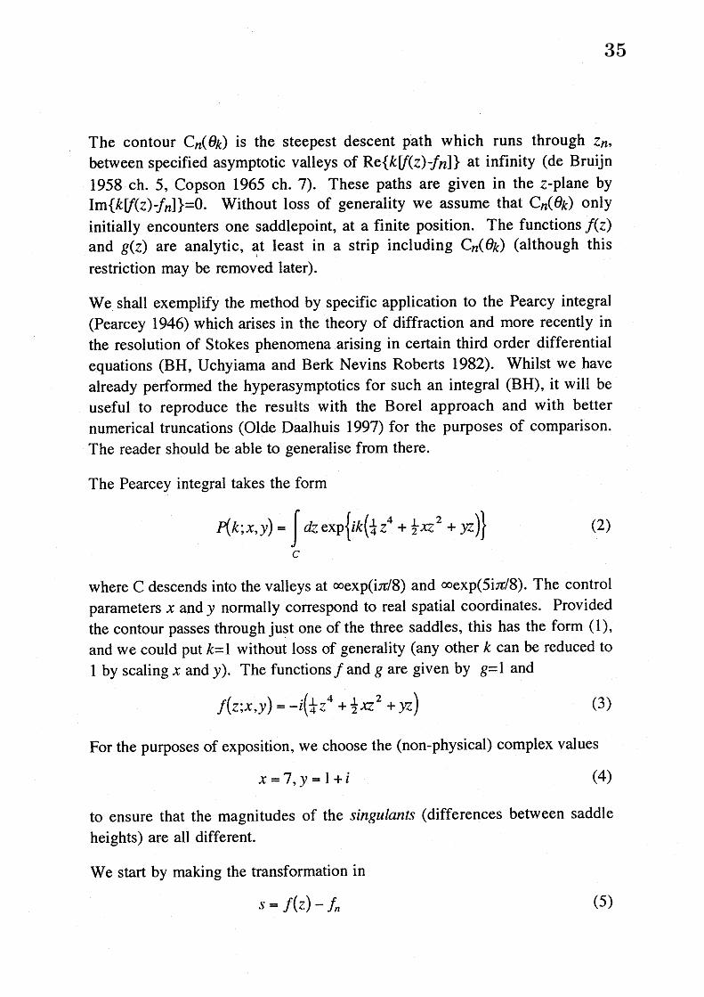
We shall exemplify the method by specific application to the Pearcy integral(Pearcey 1946) which arises in the theory of diffraction and more recently inthe resolution of Stokes phenomena arising in certain third order differentialequations ($\mathrm{B}\mathrm{H}$ , Uchyiama and Berk Nevins Roberts 1982). Whilst we havealready performed the hyperasymptotics for such an integral $(\mathrm{B}\mathrm{H})$ , it will beuseful to reproduce the results with the Borel approach and with betternumerical truncations (Olde Daalhuis 1997) for the purposes of comparison.The reader should be able to generalise from there.

The Pearcey integral takes the form

$\aleph k;\chi,y)=\int d_{Z\mathrm{x}}\mathrm{e}\mathrm{p}\mathrm{t}ik(_{4}\perp\perp)cz^{4}+2x\mathrm{z}^{2}+yz\}$(2)

where $\mathrm{C}$ descends into the valleys at $\infty\exp(\mathrm{i}\pi/8)$ and $\infty\exp(5\mathrm{i}\pi/8)$ . The controlparameters $x$ and $y$ normally correspond to $\mathrm{r}e$al spatial coordinates. Providedthe contour passes through just one of the three saddles, this has the form (1),

and we could put $k=1$ without loss of generality (any other $k$ can be reduced to

1 by scaling $x$ and $y$ ). The functions $f$ and $g$ are given by $g=1$ and

$f(_{Z;x_{\mathcal{Y}}},)=-i(_{4^{7}}\perp 4\perp 2\mathcal{Y}\sim+_{2^{X^{7}}}\sim+z)$ (3)

For the purposes of exposition, we choose the (non-physical) complex values

$x=7,\gamma=1\vee+i$ (4)

to ensure that the magnitudes of the singufants (differences between saddleheights) are all different.

We start by making the transformation in

$s=f(z)-fn$ (5)

35

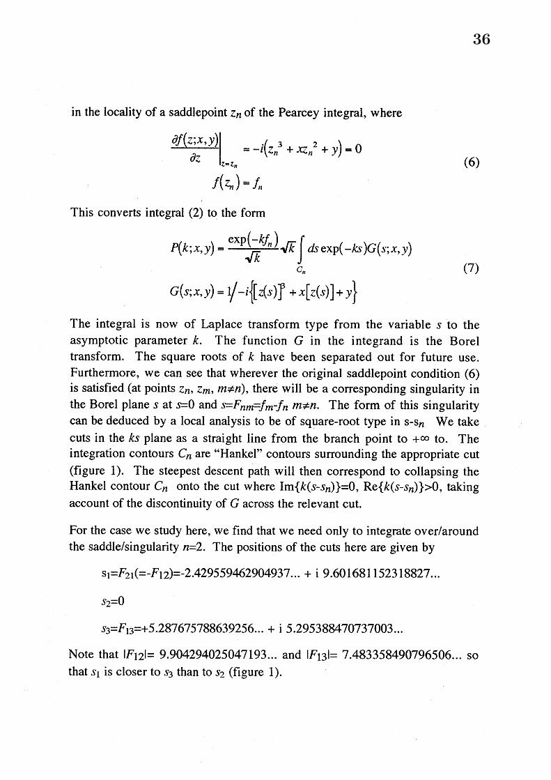
in the locality of a saddlepoint $z_{n}$ of the Pearcey integral, where

$\frac{\partial f(z^{\chi y})}{\theta_{\sim}7}.,,|_{z\approx \mathrm{z}_{n}}=-i(Z_{n}^{3}+xzn+y)20=$

(6)

$f(z_{n})=f_{n}$

This converts integral (2) to the form

$P(k;x_{\mathcal{Y}},)= \frac{\exp(-kf_{n})}{\sqrt{k}}\sqrt{k}\int_{Cn}\phi\exp(-kS)G(s;x,y)$

(7)

$G(s;x,y)=1/-i\{[z(s)\mathrm{J}+x[Z(_{S)]}+\mathcal{Y}\}$

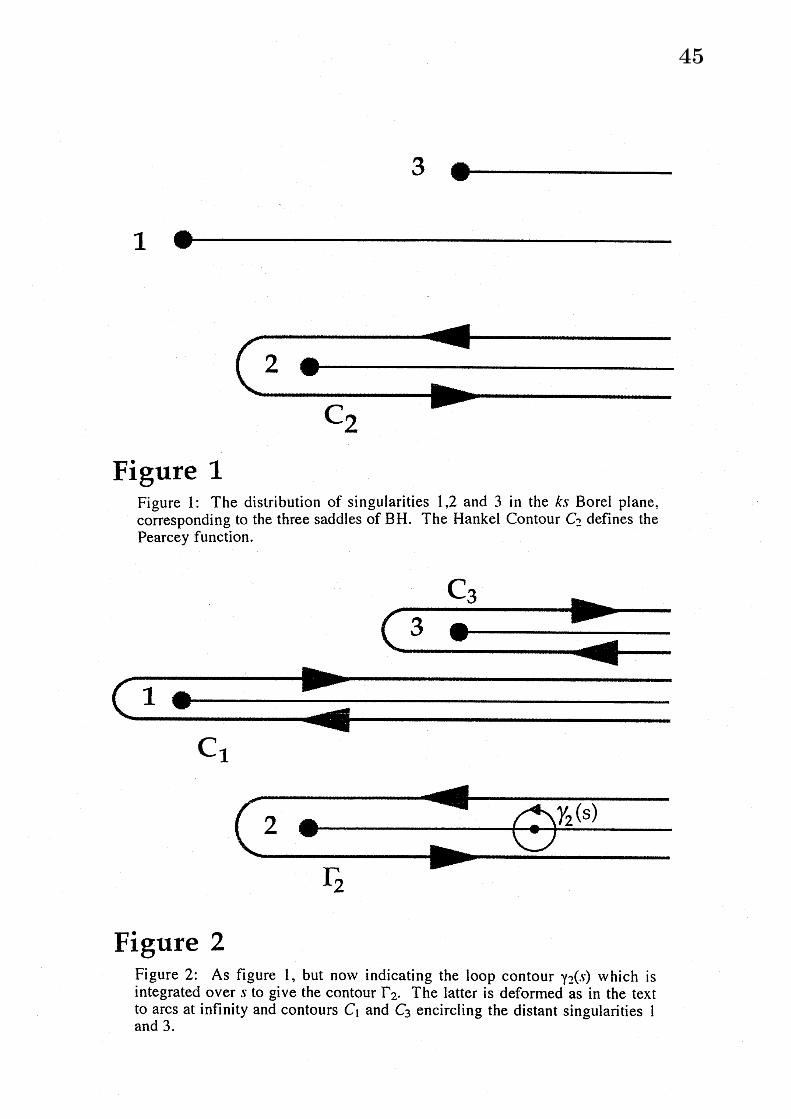
The integral is now of Laplace transform type from the variable $s$ to theasymptotic parameter $k$ . The function $G$ in the integrand is the Boreltransform. The square roots of $k$ have been separated out for future use.Furthermore, we can see that wherever the original saddlepoint condition (6)is satisfied (at points $z_{n},$ $zm,$ $m\neq n$), there will be a corresponding singularity inthe Borel plane $s$ at $s=0$ and $S=F_{nm}=fm^{fm\neq}-nn$ . The form of this singularitycan be deduced by a local analysis to be of square-root type in $\mathrm{s}- \mathrm{s}_{n}$ We takecuts in the $ks$ plane as a straight line from the branch point $\mathrm{t}\mathrm{o}+\infty$ to. Theintegration contours $C_{n}$ are “Hankel” contours surrounding the appropriate cut(figure 1). The steepest descent path will then correspond to collapsing theHankel contour $C_{n}$ onto the cut where ${\rm Im}\{k(s- s_{n})\}=0,$ ${\rm Re}\{k(s-sn)\}>0$ , takingaccount of the discontinuity of $G$ across the relevant cut.

For the case we study here, we find that we need only to integrate $\mathrm{o}\mathrm{v}\mathrm{e}\mathrm{r}/\mathrm{a}\mathrm{f}\mathrm{o}\mathrm{u}\mathrm{n}\mathrm{d}$

the $\mathrm{s}\mathrm{a}\mathrm{d}\mathrm{d}\mathrm{l}\mathrm{e}/\mathrm{s}\mathrm{i}\mathrm{n}\mathrm{g}\mathrm{u}\mathrm{l}\mathrm{a}\mathrm{r}\mathrm{i}\mathrm{t}\mathrm{y}n=2$ . The positions of the cuts here are given by

$\mathrm{S}_{1^{=F}21}(=- F_{1}2)=- 2.429559462904937\ldots+\mathrm{i}$ 9.601681152318827...

$s_{2}=0$

$s_{3}=F_{1}3^{=}+5.287675788639256\ldots+\mathrm{i}$ 5.295388470737003...

Note that I $F_{12}1=$ 9.904294025047193... and $1F_{13}|=7.483358490796506\ldots$ sothat $s_{1}$ is closer to $s_{3}$ than to $s_{?,\sim}$ (figure 1).

36

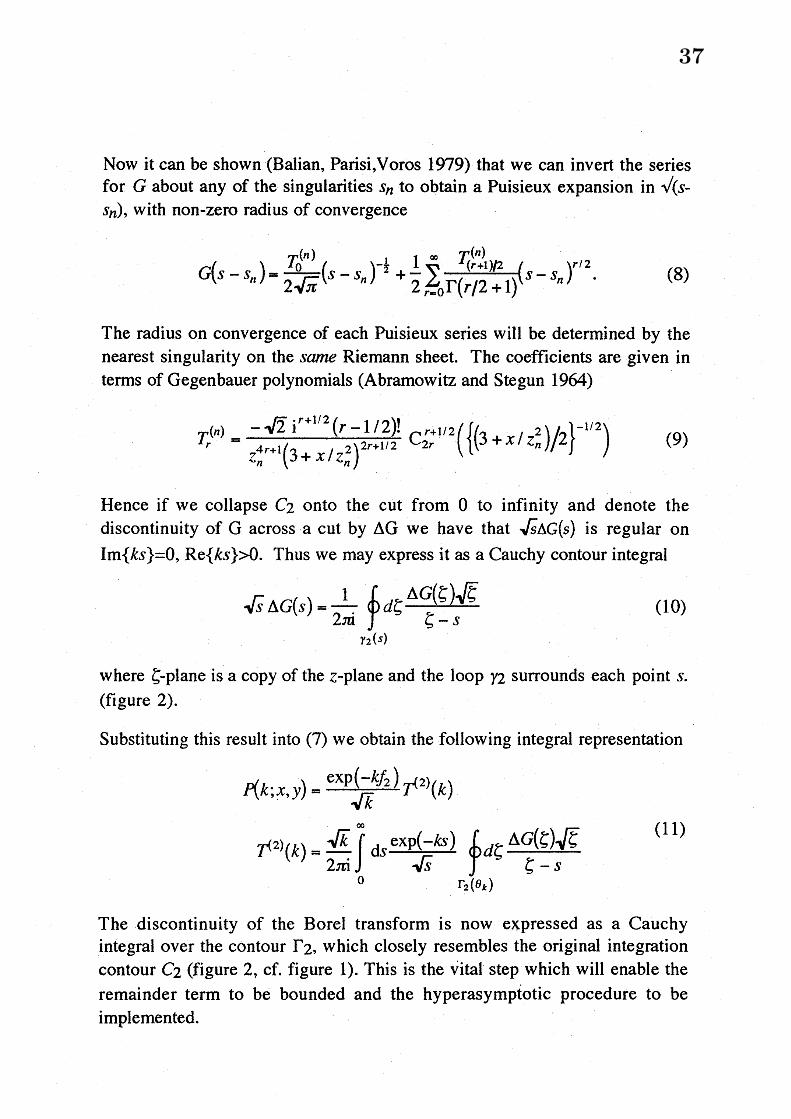
Now it can be shown (Balian, Parisi,Voros 1979) that we can invert the seriesfor $G$ about any of the singularities $s_{n}$ to obtain a Puisieux expansion in $\sqrt(S-$

$s_{n})$ , with non-zero radius of convergence

$G(s-s)n=^{\frac{T_{0}^{(n)}}{2\sqrt{\pi}}(_{S}}-Sn)^{-\mathrm{z}}1+ \frac{1}{2}\sum r\mapsto 0\infty\frac{T_{(\Gamma+}^{()}n1)l2}{\Gamma(_{\Gamma/2}+1)}(S-S_{n})^{\gamma}\mathit{1}2$. (8)

The radius on convergence of each Puisieux series will be determined by thenearest singularity on the same Riemann sheet. The coefficients are given interms of Gegenbauer polynomials (Abramowitz and Stegun 1964)

$T_{\gamma}^{(n}= \frac{-\sqrt{2}\mathrm{i}^{r+1/2}(r-1/2)!}{Z_{n}^{4r+1}(3+X/z)n22r+1’ 2})\mathrm{C}2_{\Gamma(\{)/\}^{1})}^{+1/}\Gamma 2(3+\chi/\mathrm{Z}_{n}^{2}2-/2$$(9\rangle$

Hence if we collapse $C_{2}$ onto the cut from $0$ to infinity and denote thediscontinuity of $\mathrm{G}$ across a cut by $\Delta \mathrm{G}$ we have that $\sqrt{s}\Delta G(S)$ is regular on${\rm Im}\{k_{S}\}=0,$ ${\rm Re}\{ks\}>0$ . Thus we may express it as a Cauchy contour integral

$\sqrt{s}\Delta G(S)=\frac{1}{2J\dot{\mathrm{u}}}\gamma\oint_{2(s)}d\zeta\frac{\Delta G(\zeta)\sqrt{\zeta}}{\zeta-s}$(10)

where $\zeta$-plane is a copy of the $z$-plane and the loop $\gamma_{2}$ surrounds each point $s$.(figure 2).

Substituting this result into (7) we obtain the following integral representation

flk; $X,y$) $= \frac{\exp(-kf_{2})}{\sqrt{k}}\tau^{(2}()k)$

$\tau^{(2)}(k)=\frac{\sqrt{k}}{2\pi \mathrm{i}}\int_{0}\mathrm{d}\infty S^{\frac{\exp(-ks)}{\sqrt{s}}\oint_{)}\frac{\Delta G(\zeta)\sqrt{\zeta}}{\zeta-s}}\Gamma_{2}\mathrm{t}\theta kd\zeta$

(11)

The discontinuity of the Borel transform is now expressed as a Cauchyintegral over the contour $\Gamma_{2}$, which closely resembles the original integrationcontour $C_{2}$ (figure 2, cf. figure 1). This is the vital step which will enable theremainder term to be bounded and the $\mathrm{h}\mathrm{y}\mathrm{P}^{\mathrm{e}}\mathrm{r}\mathrm{a}\mathrm{S}\mathrm{y}\mathrm{m}\mathrm{P}\grave{\mathrm{t}}\mathrm{o}\mathrm{t}\mathrm{i}\mathrm{c}$ procedure to beimplemented.

37

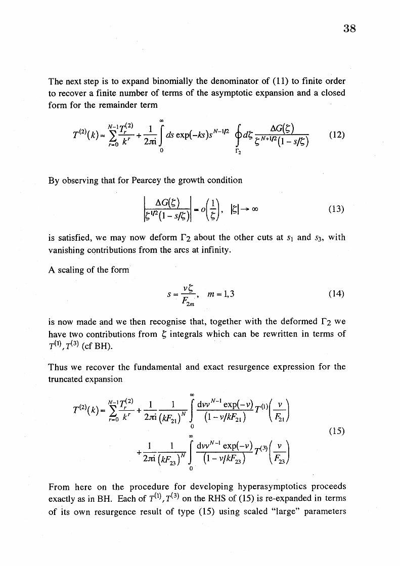
The next step is to expand binomially the denominator of (11) to finite orderto recover a finite number of terms of the asymptotic expansion and a closedform for the remainder term

$\tau^{(2)}(k)=\sum^{-1}N\gamma-0\frac{T_{r}^{(2)}}{k^{r}}+\frac{1}{2\pi \mathrm{i}}\int_{0}^{\infty}\phi e\mathrm{x}\mathrm{p}(-h)_{S^{N-1}}p\oint_{\mathrm{r}_{\sim}},d\zeta\frac{\Delta G(\zeta)}{\zeta^{N+1p}(1-s/\zeta)}$ (12)

By observing that for Pearcey the growth condition

$|\zeta|arrow\infty$ (13)

is satisfied, we may now deform $\Gamma_{2}$ about the other cuts at $s_{1}$ and $s_{3}$ , withvanishing contributions from the arcs at infinity.

A scaling of the form

$s= \frac{v\zeta}{F_{2m}}$ , $m=1,3$ (14)

is now made and we then recognise that, together with the deformed $\Gamma_{\wedge}’$’ wehave two contributions from $\zeta$ integrals $\mathrm{w}.\mathrm{h}$ich can be rewritten in terms of$\tau^{(1)},T^{\mathrm{t}3})$ (cf $\mathrm{B}\mathrm{H}$).

Thus we recover the fundamental and exact resurgence expression for thetruncated expansion

$T^{(2)}(k)= \sum_{=r0}^{N1}-\frac{\tau_{r}^{\mathrm{t}2})}{k^{r}}+\frac{1}{2\pi \mathrm{i}}\frac{1}{(kF_{21})^{N}}\int_{0}^{\infty}\frac{\mathrm{d}\mathcal{V}\mathcal{V}^{N- 1}\exp(-\mathcal{V})}{(1-v/kF_{2})1}\tau(1)(\frac{v}{F_{21}}1$

(15)

$+ \frac{\mathrm{I}}{2\pi \mathrm{i}}\frac{1}{(kF_{\mathrm{Z}3})^{N}}\int^{\infty}\frac{\mathrm{d}_{\mathcal{V}\mathcal{V}^{N-1}}\exp(_{-}\mathcal{V})}{(1-v/kF_{2})3}\tau^{(}03)(\frac{v}{F_{23}}1$

From here on the procedure for developing hyperasymptotics proceedsexactly as in $\mathrm{B}\mathrm{H}$ . Each of $\tau^{(1)},T^{(3}$ ) on the RHS of (15) is $\mathrm{r}e$-expanded in terms

of its own resurgence result of type (15) using scaled “large” parameters

38

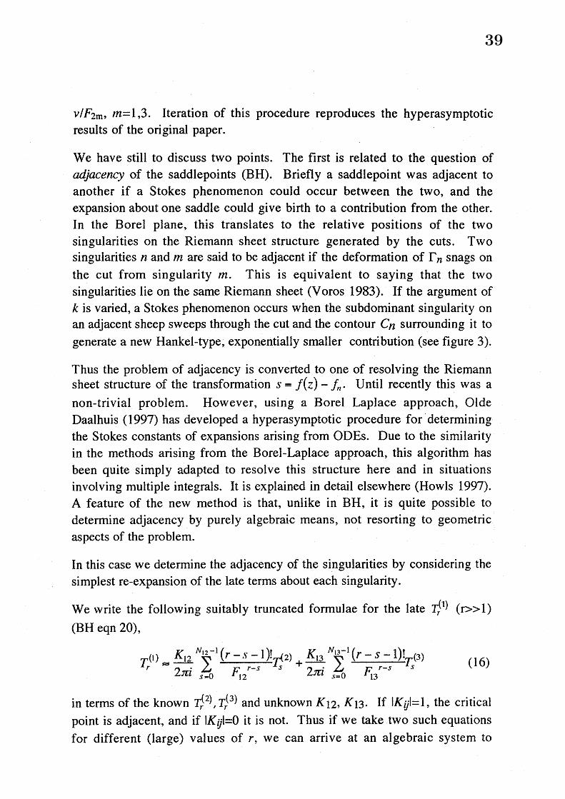
$v/F_{2\mathrm{m}},$ $m=1,3$ . Iteration of this procedure reproduces the hyperasymptotic$\mathrm{r}e$sults of the original paper.

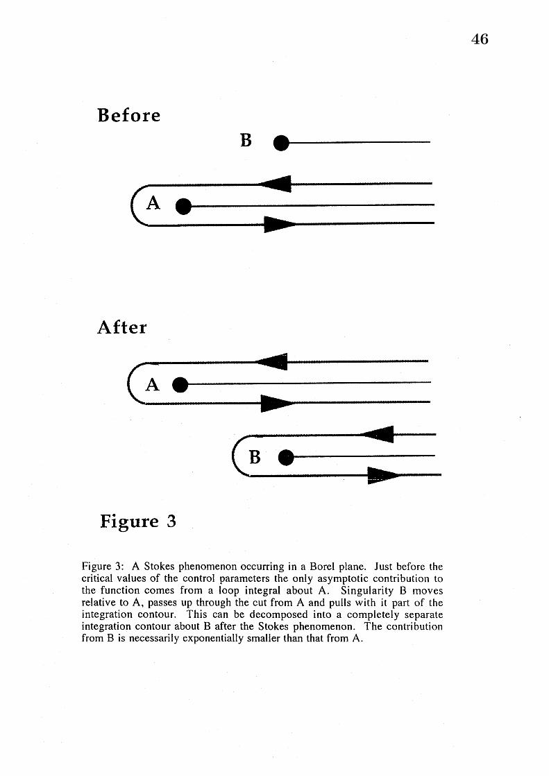
We have still to discuss two points. The first is related to the question ofadjacency of the saddlepoints $(\mathrm{B}\mathrm{H})$ . Briefly a saddlepoint was adjacent toanother if a Stokes phenomenon could occur between the two, and theexpansion about one saddle could give birth to a contribution from the other.In the Borel plane, this translates to the relative positions of the twosingularities on the Riemann sheet structure generated by the cuts. Twosingularities $n$ and $m$ are said to be adjacent if the deformation of $\Gamma_{n}$ snags onthe cut from singularity $m$ . This is equivalent to saying that the twosingularities lie on the same Riemann sheet (Voros 1983). If the argument of$k$ is varied, a Stokes phenomenon occurs when the subdominant singularity onan adjacent sheep sweeps through the cut and the contour $c_{n}$ surrounding it togenerate a new Hankel-type, exponentially smaller contribution (see figure 3).

Thus the problem of adjacency is converted to one of resolving the Riemannsheet structure of the transformation $s=f(\sim 7)-fn$ . Until recently this was anon-trivial problem. However, using a Borel Laplace approach, OldeDaalhuis (1997) has developed a hyperasymptotic procedure for determiningthe Stokes constants of expansions arising from ODEs. Due to the similarityin the methods arising from the Borel-Laplace approach, this algorithm hasbeen quite simply adapted to resolve this structure here and in situationsinvolving multiple integrals. It is explained in detail elsewhere (Howls 1997).

A feature of the new method is that, unlike in $\mathrm{B}\mathrm{H}$ , it is quite possible todetermine adjacency by purely algebraic means, not resorting to geometricaspects of the problem.

In this cas$e$ we determine the adjacency of th$e$ singularities by considering thesimplest $\mathrm{r}\mathrm{e}$-expansion of the late terms about each singularity.

We write the following suitably truncated formulae for the late $T_{r}(1)(\mathrm{r}>>1)$

(BH eqn 20),

$\tau_{\Gamma}^{(1)}\approx^{\frac{K_{12}}{2\pi i}\sum_{=}^{1}\frac{(r-s-1)!}{F_{12}r-S}}N2^{-}1S0T_{S}+\frac{K_{13}}{2\pi i}(2)\sum_{S\Rightarrow 0}^{N_{13^{-1}}}\frac{(r-s-1)!}{F_{13}r-S}\tau^{(3)}s$ (16)

in terms of the known $T_{r}^{(2)},\tau_{r}(3)$ and unknown $K_{12},$ $K_{13}$ . If $1K_{lj}\mathfrak{l}=1$ , the criticalpoint is adjac$e\mathrm{n}\mathrm{t}$ , and if $\mathrm{I}K_{\iota j}|=0$ it is not. Thus if we take two such equationsfor different (large) values of $r$ , we can arrive at an algebraic system to

39

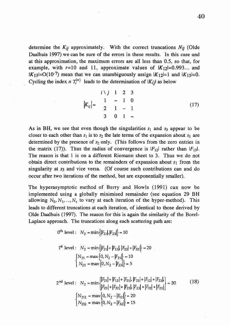
determine the $K_{\iota j}$ approximately. With the correct truncations $N_{\iota j}$ (Olde

Daalhuis 1997) we can be sure of the errors in these results. In this case andat this approximation, the maximum errors are all less than 0.5, so that, forexample, with $r=10$ and 11, approximate values of $\mathrm{I}K_{12}|=0.993\ldots$ and$\mathrm{I}K_{13}|=\mathrm{O}(10^{-7_{)}}$ mean that we can unambiguously assign $1K_{12}|=1$ and $|K_{13^{1=}0}$ .Cycling the index. $nT_{r}^{(n)}|\mathrm{l}\mathrm{e}\mathrm{a}\mathrm{d}\mathrm{s}$ to the determination of $1K_{ij}\mathrm{I}$ as below

$i\backslash j$ 1 2 31 1 $0$

$|K_{ij}|=$ (17)2 1 13 $0$ 1 -

As in $\mathrm{B}\mathrm{H}$ , we see that even though the singularities $s_{1}$ and $s_{3}$ appear to becloser to each other than $s_{1}$ is to $s_{2}$ the late terms of the expansion about $s_{1}$ aredetermined by the presence of $s_{2}$ only. (This follows from the $\mathrm{z}e$ro entries inthe matrix (17)$)$ . Thus the radius of convergence is $\mathrm{I}F_{12}1$ rather than I $F_{13}1$ .The reason is that 1 is on a different Riemann sheet to 3. Thus we do notobtain direct contributions to the remainders of expansion about $s_{1}$ from thesingularity at $s_{3}$ and vice versa. (Of course such contributions can and dooccur after two iterations of the method, but are exponentially smaller).

The hyperasymptotic method of Berry and Howls (1991) can now beimplemented using a globally minimised remainder (see equation 29 BHallowing $N_{0},$ $N_{1},$ $\ldots,N_{s}$ to vary at each iteration of the hyper-method). Thisleads to different truncations at each iteration, of identical to those derived byOlde Daalhuis (1997). The reason for this is again the similarity of the Borel-Laplace approach. The truncations along each scattering path are:

$0^{\mathrm{t}\mathrm{h}}$ level : $N_{2}=\mathrm{m}\dot{\mathrm{m}}\{|\mathrm{r}_{21}\ovalbox{\tt\small REJECT}|\mathrm{p}_{23}|\}=10$

1st level: $N_{2}= \min\{|F21|+|F_{12}$ } $|F_{23}|+|F_{32}|\}=20$

$\{$

$N_{21}= \max\{0,$ $N_{2^{-}}|F_{21}|\}=10$

$N_{23}= \max\{0,N_{2}-|F_{23}|\}=5$

$2^{\mathrm{n}\mathrm{d}}$ level: $N_{2}= \min=30$ (18)

$\{_{N_{\mathfrak{B}}=}^{N_{212}=}2\mathrm{t}\max_{\max \mathrm{o}_{J}N}0,N_{2^{-}}2^{-|}|FF_{3}122\#_{=1}=205$

40

These values of the truncations should be contrasted with equation (44) of $\mathrm{B}\mathrm{H}$ .Note that the $\mathrm{o}\mathrm{v}e$ rall numerical accuracy is much greater with the bettertruncatio.ns, even after the 2nd hyperasymptotic stage. In BH we used threeiterations to achieve an accuracy of $\mathrm{O}(10^{- 1}2)$ but here we reach $\mathrm{O}(10^{- 1}6)$ afterthe second iteration. Note however that with the new truncations we haveused more than twice the number of terms. The hyperterminants have beencalculated according to $\mathrm{t}\mathrm{h}’ \mathrm{e}$ algorithm of Olde Daalhuis (1997a).

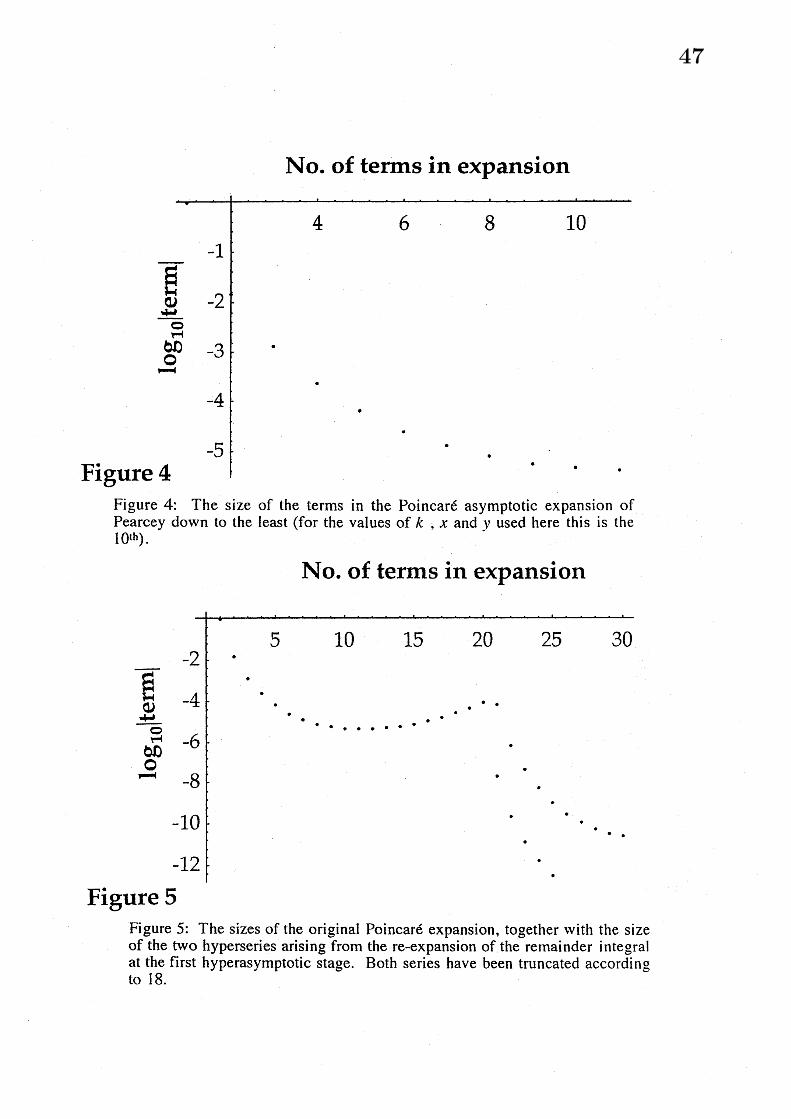
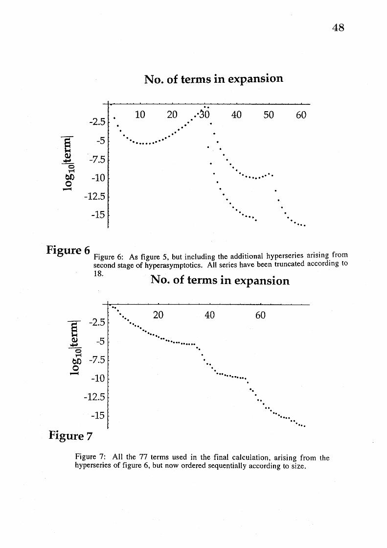
Figures 4, 5 and 6 illustrate the hyperasymptotics stages recalculated here.Figure 7 shows the decay of the terms by modulus.

Generalisations

The calculations performed here have brought the results of BH up to date.They have also illustrated the new general approach to hyperasymptotics usingthe Borel-Laplace technique. This technique appears to be quite general.Similar $\mathrm{r}e$sults are obtained by Olde Daalhuis (1997) for higher order rankone equations. An application along these lines to eigenvalue asymptotics hasalso been made (Alvarez, Howls, Silverstone 1997), giving rise to new formsof the hyperterminants. Since the Pearcey integral satisfies a partialdifferential equation (Connor and Curtis 1984) we tentatively suggest that acareful analysis of certain classes of PDE’s in the appropriate complex planemight also generate a hyperasymptotic procedure. Other areas of applicationinclude nonlinear differential equations, difference equations and multipleinte.grals (Howls 1997). It is hoped to use the Borel-Laplace approach to studythe coalescence of singularities in greater detail (thereby extending the workof Berry and Howls 1993, $1994\mathrm{a}$).

Acknowledgements

The author would like to express his thanks to The Royal Society, The NewtonInstitute, JSPS, RIMS and to Professors Kawai and Takei for their generoushospitality whilst attending this conference.

41

References

Abramowitz, M. and Stegun, I.A. 1964, Handbook ofmathematicalfimctions(National Bureau of Standards, Washington).

Alvarez, G., Howls C.J., Silverstone H. 1997, In preparation.

Aoki T., Kawai T., Takei Y. 1994, in M\’ethodes r\’esurgentes, Analysealg\’ebraique des perturbations singulieres, ed. L.Boutet de Monvel (Hermann)

Balian, R., Parisi, G. and Voros, A. 1979, Phys. Rev. Lett. 41, 141-144.

Berk, H.L., Nevins, W.M., and Roberts, $\mathrm{K}.\mathrm{V}$ . 1982, J. Maths. Phys. 23,. 988-1002.

Berry, $\mathrm{M}.\mathrm{V}$ . 1989, Proc. $Roy$. Soc. Lond, A422, 7-21.

Berry, $\mathrm{M}.\mathrm{V}$ . $1990\mathrm{a}$ , Proc. $Roy$ . Soc. Lond, A427, 265-280.

Berry, $\mathrm{M}.\mathrm{V}$ . $\mathrm{I}990\mathrm{b}$ , Proc. $Roy$ . Soc. Lond, A429, 61-72.

Berry, $\mathrm{M}.\mathrm{V}$ . $1991\mathrm{a}$ , Proc. $Roy$ . Soc. Lond, A434, 465-472.

Berry, $\mathrm{M}.\mathrm{V}$ . $1991\mathrm{b}$ , Proc. $Roy$. Soc. Lond, A435, 437-444.

Berry, $\mathrm{M}.\mathrm{V}$ . and Howls, $\mathrm{C}.\mathrm{J}$ . 1990, Proc. $Roy$ . Soc. Lond., A430, 653-668.

Berry, $\mathrm{M}.\mathrm{V}$ . and Howls, $\mathrm{C}.\mathrm{J}$ . 1991, Proc. $Roy$ . Soc. Lond., A434, 657-675(Reference BH of the text).

Berry, $\mathrm{M}.\mathrm{V}$ . and Howls, $\mathrm{C}.\mathrm{J}$ . 1993, Proc. $Roy$ . Soc. Lond., A443, 107-126

Berry, $\mathrm{M}.\mathrm{V}$ . and Howls, $\mathrm{C}.\mathrm{J}$ . $1994\mathrm{a}$ , Proc. $Roy$ . Soc. Lond., A444, 201-216

Berry, $\mathrm{M}.\mathrm{V}$ . and Howls, $\mathrm{C}.\mathrm{J}$ . $1994\mathrm{b}$ , Proc. $Roy$. Soc. Lond., A447, 527-555

Boyd, $\mathrm{W}.\mathrm{G}$.C. 1990, Proc. $Roy$. Soc. Lond., A429, 227-246.

Boyd, $\mathrm{W}.\mathrm{G}$ .C. 1993, Proc. $Roy$ . Soc. Lond., A440, 493-518.

Chapman, S. J. 1996, Proc. $Roy$ . Soc. Lond. $\mathrm{A}$ , in press

Connor $\mathrm{J}.\mathrm{N}$ .L. and Curtis $\mathrm{P}.\mathrm{R}$ . 1984, J. Maths. Phys. 25, 2895-2902

42

Copson, E.T 1965, Asymptotic expansions (Cambridge University Press).

De Bruijn, $\mathrm{N}.\mathrm{J}$ . 1958, Asymptotic methods in analysis (North-Holland,Amsterdam).

Dingle, $\mathrm{R}.\mathrm{B}$ . 1973, Asymptotic expansions: their derivation andinterpretation (Academic Press: New York and London).

\’Ecalle, J. 1981, Les fonctions r\’esurgentes (3 volumes) Publ. Math.Universit\’e de Paris-Sud.

\’Ecalle, J. 1984, Cinq applications des fonctions r\’esurgentes, Preprint$84\mathrm{T}62$ , Orsay.

Howls, C. J., 1993, Proc. $Roy$ . Soc. Lond., A439, 373-396.

Howls, C. J., 1997, preprint, Brunel University, $\mathrm{U}\mathrm{K}$ .

Hardy, G. H. 1949, Divergent Series, (Clarendon Press Oxford)

Jones, $\mathrm{D}.\mathrm{S}$ . 1990 in Proc. Int. Symp.Asymp. &Comp. Anal. (ed. R. Wong),pp241-264. (New York: Marcel Dekker)

$\mathrm{M}\mathrm{c}\mathrm{L}\mathrm{e}\mathrm{o}\mathrm{d},$ $\mathrm{J}.\mathrm{B}$ . 1992, Proc. $Roy$ . Soc. Lond., A437, 343-354.

Olde Daalhuis, A.B 1992, IMA J. Appl. Math. 49, 203-216

Olde Daalhuis, A.B 1995, Methods Appl. Anal. 2, 198-211

Olde Daalhuis, A.B 1997, preprint, University of Edinburgh, $\mathrm{U}\mathrm{K}$ .

Olde Daalhuis (1997a), Hyperterminants ,preprint,Univ. of Edinburgh, UK

Olde Daalhuis, $\mathrm{A}.\mathrm{B}$ . and Olver, $\mathrm{F}.\mathrm{W}$.J. 1994, Proc. $Roy$. Soc. Lond. A445,39-56.

Olde Daalhuis, $\mathrm{A}.\mathrm{B}$ . and Olver, $\mathrm{F}.\mathrm{W}$ .J. 1995, Methods Appl. Anal. 2, 173-197.

Olver, $\mathrm{F}.\mathrm{W}$.J. 1990, in Proc. Int. Symp.Asymp. &Comp. Anal. (ed. R.Wong), pp329-355. (New York: Marcel Dekker).

Olver, $\mathrm{F}.\mathrm{W}$.J. $1991\mathrm{a}$ , SIAM J. Math. Anal. 22, 1460-1474.

43

Olver, $\mathrm{F}.\mathrm{W}$ .J. $1991\mathrm{b}$ , SIAM J. Math. Anal. 22, 1475-1489.

Paris R.B., $1992\mathrm{a}$ J. Comp.Appl. Math. 41, 117-133.

Paris R.B., $1992\mathrm{b}$ , Proc. $Roy$. Soc. Lond., A436, 165-186.

Pearcey, T. 1946 Phil. $\mathrm{M}\mathrm{a}\mathrm{g}$.$37$’ 311-317.

Stokes, $\mathrm{G}.\mathrm{G}$ . 1847, Trans. Camb. Phil. Soc. 9, 379$A07$ , reprinted inMathematical and Physical papers by the late Sir George GabrielStokes (Cambridge University Press 1904) $\mathrm{v}\mathrm{o}\mathrm{l}\mathrm{I}\mathrm{I}$ , 329-357.

Stokes, $\mathrm{G}.\mathrm{G}$ . 1864, Trans.Camb.Phil.Soc. 10, 106-128, reprinted inMathematical and Physical papers by the late Sir George Gabriel Stokes(Cambridge University Press 1904) vol.IV, 77-109.

Uchiyama K. 1994, in M\’ethodes r\’esurgentes, Analyse alg\’ebraique desperturbations singulieres, ed. L.Boutet de Monvel (Hermann)

Voros, A. 1983 Ann. Inst. Henri Poincar\’e 39, 211-338

44

3

1

Figure 1Figure 1: The distribution of singularities 1,2 and 3 in the $k.\backslash \cdot$ Borel plane.corresponding to the three saddles of $\mathrm{B}\mathrm{H}$ . The Hankel Contour $C_{-}$, defines thePearcey function.

Figure 2Figure 2: As figure 1, but now indicating the loop contour $\mathrm{Y}_{-}’’(.\mathrm{S})$ which isintegrated over $s$ to give the contour $\Gamma_{2}$ . The latter is deformed as in the textto arcs at infinity and contours $C_{1}$ and $C_{3}$ encircling the distant singularities 1and 3.

45

Before$\mathrm{B}$

After

Figure 3

Figure 3: A Stokes phenomenon occurring in a Borel plane. Just before thecritical values of the control parameters the only asymptotic contribution tothe function comes from a loop integral about A. Singularity $\mathrm{B}$ movesrelative to $\mathrm{A}$ , passes up through the cut from A and pulls with it part of theintegration contour. This can be decomposed into a completely separateintegration contour about $\mathrm{B}$ after the Stokes phenomenon. The contributionfrom $\mathrm{B}$ is necessarily exponentially smaller than that from A.

46

No. of terms in expansion

Figure 4: The size of the terms in the Poincar\’e asymptotic expansion ofPearcey down to the least (for the values of $k$ , $x$ and $v$ used here this is the$10^{\iota \mathrm{h}})$ .

No. of terms in expansion

Figure 5: The sizes of the original Poincar\’e expansion, together with the sizeof the two hyperseries arising from the $\mathrm{r}\mathrm{e}$-expansion of the remainder integralat the first hyperasymptotic stage. Both series have been truncated accordingto 18.

47

No. of terms in expansion

$\underline{\not\in\omega}$

$\underline{\mathrm{b}\mathrm{O}}\frac{\mathrm{o}}{\mathrm{D}}$

Figure 6Figure 6: As figure 5, but including the additional hyperseries arising fromsecond stage of hyperasymptotics. All series have been truncated according to18. No. of terms in expansion

Figure 7: All the 77 terms used in the final calculation, $\mathrm{a}\mathrm{r}\mathrm{i}\sin\sigma\circ$ from thehyperseries of figure 6, but now ordered sequentially according to size.

48