Uses and abuses of EIDORS: An extensible software … and abuses of EIDORS: An extensible software...
21
Uses and abuses of EIDORS: An extensible software base for EIT Andy Adler 1 , William R. B. Lionheart 2 1 School of Information Technology and Engineering, University of Ottawa, Canada 2 School of Mathematics, University of Manchester, U.K. E-mail: [email protected], [email protected] Abstract. EIDORS is an open source software suite for image reconstruction in electrical impedance tomography and diffuse optical tomography, designed to facilitate collaboration, testing and new research in these fields. This paper describes recent work to redesign the software structure in order to simplify its use and provide a uniform interface, permitting easier modification and customization. We describe the key features of this software, followed by examples of its use. One general issue with inverse problem software is the difficulty of correctly implementing algorithms, and the consequent ease with which subtle numerical bugs can be inadvertently introduced. EIDORS helps with this issue, by allowing sharing and reuse of well documented and debugged software. On the other hand, since EIDORS is designed to facilitate use by non-specialists, its use may inadvertently result in such numerical errors. In order to address this issue, we develop a list of ways in which such errors with inverse problems (which we refer to as “cheats”) may occur. Our hope is that such an overview may assist authors of software to avoid such implementation issues. Keywords : Electrical Impedance Tomography, Open Source, Inverse Problems 1. Introduction EIDORS (Electrical Impedance and Diffuse Optical tomography Reconstruction Software) is a software suite for image reconstruction in electrical impedance tomography (EIT) and diffuse optical tomography (DOT). Its goal is to provide a freely distributable and modifiable software for image reconstruction of electrical or diffuse optical data. Such software facilitates research and development in these fields by providing a reference implementation against which new developments can be compared, and by providing a functioning software base from which new ideas may be built and tested. Making the source code available also facilitates scrutiny of algorithms and their implementation by other researchers. The original EIDORS (version 1) software [17] is based on software from the thesis of Vaukhonen [16]. It implemented a MATLAB package for two-dimensional mesh generation, solving of the forward problem and reconstruction and display of the images. In order to provide capability to solve 3D reconstruction models, a new project, EIDORS3D (version 2), was begun [11], based on
-
Upload
hoanghuong -
Category
Documents
-
view
215 -
download
1
Transcript of Uses and abuses of EIDORS: An extensible software … and abuses of EIDORS: An extensible software...
Uses and abuses of EIDORS: An extensible software
base for EIT
Andy Adler1, William R. B. Lionheart2
1 School of Information Technology and Engineering, University of Ottawa, Canada2 School of Mathematics, University of Manchester, U.K.
E-mail: [email protected], [email protected]
Abstract.EIDORS is an open source software suite for image reconstruction in electrical
impedance tomography and diffuse optical tomography, designed to facilitatecollaboration, testing and new research in these fields. This paper describes recentwork to redesign the software structure in order to simplify its use and provide auniform interface, permitting easier modification and customization. We describe thekey features of this software, followed by examples of its use. One general issue withinverse problem software is the difficulty of correctly implementing algorithms, and theconsequent ease with which subtle numerical bugs can be inadvertently introduced.EIDORS helps with this issue, by allowing sharing and reuse of well documented anddebugged software. On the other hand, since EIDORS is designed to facilitate use bynon-specialists, its use may inadvertently result in such numerical errors. In order toaddress this issue, we develop a list of ways in which such errors with inverse problems(which we refer to as “cheats”) may occur. Our hope is that such an overview mayassist authors of software to avoid such implementation issues.
Keywords : Electrical Impedance Tomography, Open Source, Inverse Problems
1. Introduction
EIDORS (Electrical Impedance and Diffuse Optical tomography Reconstruction
Software) is a software suite for image reconstruction in electrical impedance
tomography (EIT) and diffuse optical tomography (DOT). Its goal is to provide a
freely distributable and modifiable software for image reconstruction of electrical or
diffuse optical data. Such software facilitates research and development in these fields by
providing a reference implementation against which new developments can be compared,
and by providing a functioning software base from which new ideas may be built and
tested. Making the source code available also facilitates scrutiny of algorithms and their
implementation by other researchers. The original EIDORS (version 1) software [17] is
based on software from the thesis of Vaukhonen [16]. It implemented a MATLAB
package for two-dimensional mesh generation, solving of the forward problem and
reconstruction and display of the images. In order to provide capability to solve 3D
reconstruction models, a new project, EIDORS3D (version 2), was begun [11], based on
Uses and abuses of EIDORS: An extensible software base for EIT 2
the software developed for the thesis of Polydorides [12] The EIDORS software packages
shared the same numerical and algorithmic foundations, but shared very little software
code. Each software package modelled the medium under investigation using a simplex
based finite element representation, and images were reconstructed using regularized
inverse techniques.
In the three years since the publication of EIDORS3D, several patterns of use
have been noted. Researchers typically download the software, run the provided
demonstration examples, and make modifications in the demonstration examples and
the software internals to meet their needs. Because of the lack of a modular software
structure of EIDORS3D, changes tended to be made into the code itself. This
resulted in duplicated code which could not easily be refactored in order to be
contributed back to EIDORS. Additionally, recent work has begun to move away
from basic reconstruction algorithms, focussing on such issues as mesh generation,
electrode modelling, visualization and electrode error detection. Such research would
be facilitated by using modular components which could be “plugged” into a selection
of reconstruction algorithms.
To address these issues, the EIDORS software has been completely restructured
with the goal of providing an extensible software base designed to support community
use, modification and contribution. These modifications have been released as EIDORS
version 3 (currently at release 3.1), which incorporates the following features:
• Multiple algorithm support: EIDORS V.3 has been redesigned to allow flexibility of
using multiple algorithms (or parts of algorithms). This version provides access to
the algorithms of [1], [3], [11], [14] and [17]. We feel that this capability is becoming
more important with a trend toward meta-algorithms in EIT, such as algorithms
for detection of electrode errors [2].
• Generalized model formats: One limitation of previous versions of the EIDORS
software is that they were designed around specific electrode configurations and
stimulation and measurements patterns. While it was possible to use the software
for more general configurations, this was a fairly daunting task. In order to support
the wide variety of EIT measurements and algorithms, EIDORS now provides a
general EIT model format (iethe fwd model structure). Additionally, several utility
functions are provided to create common electrode and stimulation configurations.
This format specifies the electrode positions, contact impedances, and stimulation
and measurement patterns, and all supported algorithms are able to reconstruct
images based on data provided in these formats.
• Interface software for common EIT systems: functions are provided (in the interface
directory) to load from a variety of EIT hardware storage formats into the EIT
data format. Currently, EIDORS will detect when data do not match the specified
protocol in the fwd model, but will not (yet) automatically convert the data. At this
point it has only been possible for the developers to offer support for EIT hardware
that they have access to. We hope that EIDORS will attract contributions from
Uses and abuses of EIDORS: An extensible software base for EIT 3
software developers who have access to other hardware systems.
• Usage examples: It is observed that researchers typically base new software on
demonstration examples. To facilitate this, several simple and more complex usage
examples are provided for image reconstruction in two and three dimensions using
various image reconstruction algorithms and combinations of algorithms.
• Test suite: Software is intrinsically difficult to test. While little work has been
done specifically on testing numerical software for inverse problems, we believe
that such tests are even more difficult. EIDORS has begun to implement a series
of regression test scripts (in the tests directory) to allow automatic testing of
code modifications. For example the function calc jacobian test.m validates a
function to calculate the Jacobian against an approximation of the Jacobian using
the perturbation method.
• Open-source license: EIDORS is licensed under the GNU General Public License [9].
Users are free to use, modify, and distribute their modifications. All modifications
must include the source code, or instructions on how to obtain it. EIDORS may
be used in a commercial product, as long as the source code for EIDORS and all
modifications to it are made available. In addition, by making EIDORS available
in this way, we would like to encourage other authors to publish their scientific
software, in order to make results more easily verifiable and repeatable.
• Sourceforge hosting: In order to allow collaborative development, EI-
DORS is hosted by sourceforge.net available at http://eidors.org or
http://eidors3d.sf.net. Software is available for download as packaged released
versions (version 3.1 was released on 24 Jan 2006, and contains the features de-
scribed in this paper), or the latest developments may be downloaded from the
Concurrent Versions System (CVS) [4]. Sourceforge hosting allows for collabora-
tive development for group members, while permitting read-only access to everyone.
In order to become a member of the developer group, new contributors should con-
tact the authors. One concern with a distributed software project is the possibility
of conflict due to disparate authors working on the same module. Version control
software such as CVS is widely understood to facilitate collaborative development,
and manage software version conflicts [4].
• Language independence: (Octave and Matlab) EIDORS was originally written for
Matlab. However, the eventual goal is to support multiple mathematical software
packages. Some progress has been achieved, and EIDORS version 3 works with
Octave [8], although some advanced graphics functions still function only with
Matlab. The current version of EIDORS works with Octave (version ≥ 2.9.4) and
Matlab (version ≥ 6.0). Support for Octave was motivated by two goals: first,
octave provides a free software platform which can encourage the development of
embedded and commercial applications of EIT which are currently limited by the
cost of Matlab, and secondly, Octave provides an open source platform to match
the open source nature of EIDORS.
Uses and abuses of EIDORS: An extensible software base for EIT 4
• Pluggable code base: In order to facilitate user modifications, EIDORS has been
designed to provide some of the benefits of object-oriented (OO) software [10]:
abstraction, encapsulation, polymophism and inheritance. We have decided not to
use the OO framework provided by Matlab, because in our experience it is somewhat
cumbersome, and may be intimidating to many mathematicians and engineers who
do not regularly write OO software. Another issue is the unfortunate reputation
of the Matlab language for undergoing dramatic modifications to new language
features in the first few versions. For these reason, EIDORS has been designed
using a “pluggable” software approach. This design uses function pointers to allow
adding new modules and controlling which parts of functions are executed. EIDORS
is thus able to offer the OO features of packaging and polymophism, while not
encapsulation or inheritance. A detailed description of this capability is provided
in the next section. While EIDORS does not yet provide algorithms for DOT, this
aspect of the software architecture allows integration of such algorithms with the
advanced inverse solvers provided.
• Automatic matrix caching: In order to increase performance of image reconstruction
software, it is important to save and reuse values of computationally expensive
variables, such as the Jacobian and image priors. Such caching complicates the
software implementation, and potentially leads to errors. In order to simplify
design, EIDORS offers the ability to automatically detect when a calculation
requests a value previously calculated, and will automatically retrieve that previous
value. EIDORS extracts caching to a separate module eidors obj, in a way that
will generally happen transparently for the programmer. This capability helps
software based on EIDORS to be more clear and easier to decompose into functional
modules.
• Enhanced Finite Element Modelling and Graphical output: Image reconstruction,
especially in 3D, requires functions to show high quality graphical representations
of the images. EIDORS provides several functions for image presentation using
the Matlab graphics features, as well as functions to display images using
the VTK visualization program [13], after exporting the data to a vtk file.
show fem.m displays a three dimensional model of the finite element mesh and
conductivity changes, while show slices.m allows generation of images of arbitrary
two dimensional slices through a volume. Examples of these functions are
shown in Figs. 5 and 6. All EIDORS graphics functions now use a single
colour mapping function calc colours.m, which allows global modification of
all image colouring using a global variable eidors colours. For modelling, the
create tank mesh ng.m function is provided to generate a finite element mesh of a
cylindrical tank with circular of rectangular electrodes using the netgen [15] mesh
generator.
We hope that by providing a structure for community collaboration in EIT algorithms,
we can produce robust, reliable and fairly portable software which draws on our collective
Uses and abuses of EIDORS: An extensible software base for EIT 5
expertise and facilitates innovations in the field.
2. Software Architecture
This section describes the structure of EIDORS objects and their relationship to the
underlying finite element models and numerical functions.
2.1. Object Structure
EIDORS software consists of four primary objects: data, image, fwd model, inv model.
Each object is represented by a structure. All objects have the properties of a name and
type. The name is arbitrary; it is displayed by the graphics functions, and could also be
useful to distinguish objects in a user specified function. The type is used to identify
the object type (ie data, image etc.).
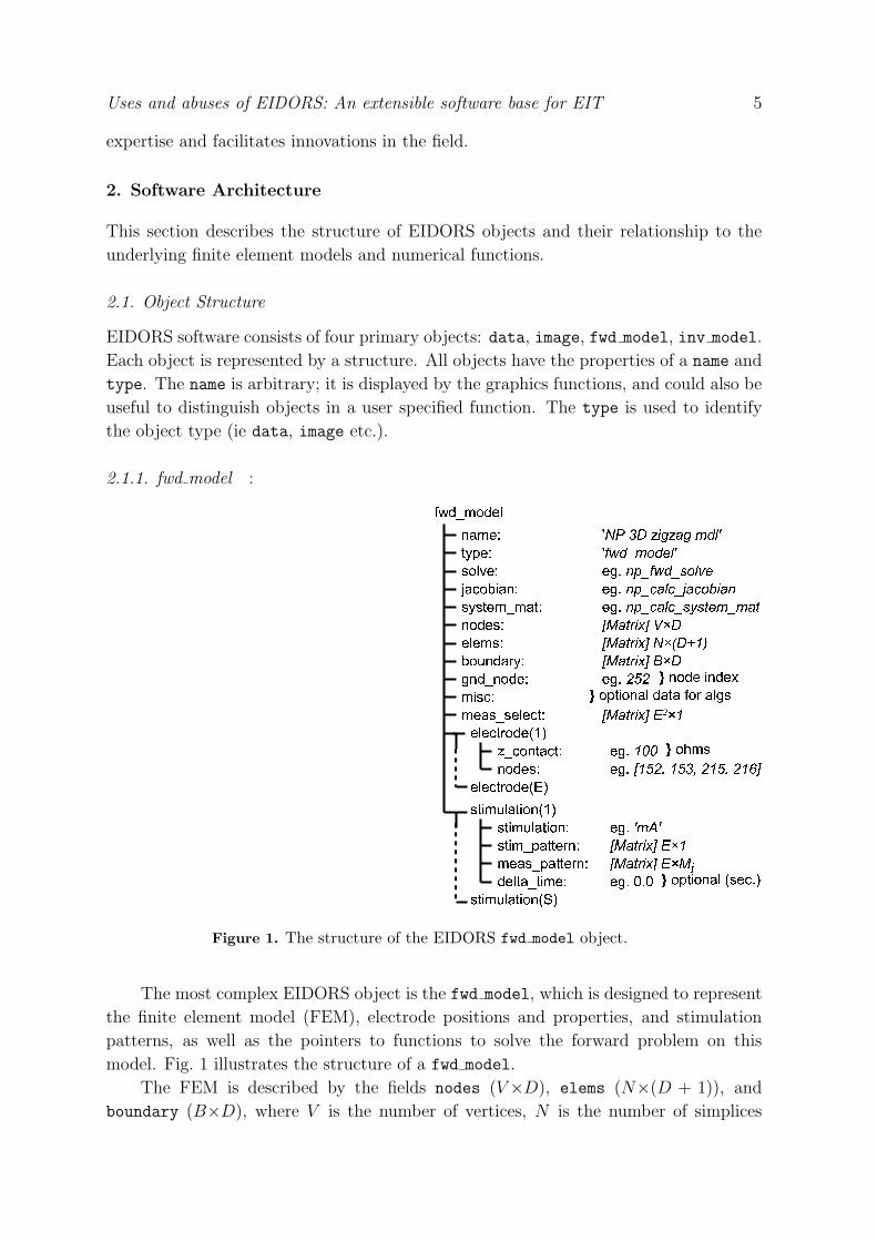
2.1.1. fwd model :
Figure 1. The structure of the EIDORS fwd model object.
The most complex EIDORS object is the fwd model, which is designed to represent
the finite element model (FEM), electrode positions and properties, and stimulation
patterns, as well as the pointers to functions to solve the forward problem on this
model. Fig. 1 illustrates the structure of a fwd model.
The FEM is described by the fields nodes (V×D), elems (N×(D + 1)), and
boundary (B×D), where V is the number of vertices, N is the number of simplices
Uses and abuses of EIDORS: An extensible software base for EIT 6
(and also the number of unknown conductivities to be solved by the inverse solution),
B the number of simplices with a face on the boundary, and D the model dimension
(D = 2 for 2D and D = 3 for 3D). The gnd node is the vertex number attached to
ground.
The electrodes are defined by a vector (E × 1) of electrode fields. Each of E
electrode objects has fields z contact (scalar) and nodes (vector) which represent the
(possibly complex) contact impedance and vertices to which that electrode is connected.
A point electrode would have a single element nodes field with z contact = 0 while
an electrode with a complete electrode model would have multiple vertices specified in
nodes and z contact ≥ 0. Note that EIDORS does not require the electrode model to
be the same for all electrodes in a fwd model.
Using these electrodes, a sequence of S stimulation patterns are applied and
measurements performed in order to generate a frame of data. Stimulation patterns
are defined by a vector (S × 1) of stimulation fields. Each stimulation object
has fields stimulation, stim pattern, and meas pattern. The stimulation is
the quantity stimulated into the electrodes. Typically, EIT systems inject current
(represented by “mA”), but the quantity could be voltage (or luminous intensity in
an optical tomography system). Currently, EIDORS only accepts current stimulations.
stim pattern is a vector (E × 1) of the stimulation quantity applied to each electrode
during that stimulation pattern. Each stimulation object also has an optional
delta time field representing the time increment between measurements at this
stimulation and the beginning of the measurement frame. Such data may be used
to perform Kalman filtering, for example. meas pattern is a (sparse) matrix (E×Mi)
representing the Mi measurement patterns for stimulation i. Each column of this matrix
represents the amplification of the signal at each electrode for a single measurement
pattern. For example if measurement k = 2 is the difference signal between electrodes
4 and 5, then meas patternj,k is 1 for j = 4, −1 for j = 5 and zero for other values
of j when k = 2. EIDORS does not require that the number of measurement patterns
be equal for each stimulation pattern. The total number of measurements per frame is
M = ΣSi=0Mi
For many EIT systems, an adjacent stimulation pattern is used with no
measurement taken at current stimulation electrodes, giving M = E × (E − 3). For
a 16 electrode system, this gives 208 measurements (or, considering reciprocity, 104
independent measurements). One practical consideration is that many EIT systems
store data as a matrix of size (E2×F ) where F is the number of data frames. In this
case E2 = 256 of which 3×E = 48 measurements in each frame yield zero. In order to
allow easy use of EIDORS with such systems, the optional field meas select (E2 × 1)
is defined for the fwd model. This field contains a 1 in each position corresponding to
a used measurement pattern in the frame (thus meas select will have M ones).
EIDORS provides several utility functions to define the fields of the fwd model
for common patterns, such as the mk circ tank.m, mk stim patterns.m and
mk common model.m functions. These functions allow easy definition of circular and
Uses and abuses of EIDORS: An extensible software base for EIT 7
cylindrical FEM models with rings of electrodes and adjacent stimulation protocols.
The fwd model contains three function pointers to allow solution of the forward
problem, solve, jacobian and system mat. Each field contains the function name
(as a string) or a function pointer to calculate these quantities. In each case, these
quantities are solved using the utility functions fwd solve(), calc jacobian() and
calc system mat(). For example, given a fwd model object fmdl, we may calculate
the system matrix, Smat, using:
Smat = calc_system_mat( fmdl );
This code will call the appropriate function and also manage the caching of the
computed result. In this case, if a system matrix has previously been computed for a
fwd model object with the same values as fmdl, then the previous result will be returned,
without the computation function being called.
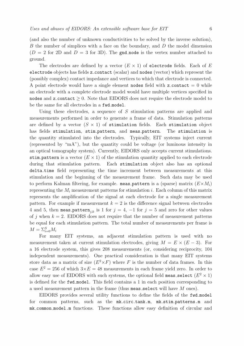
2.1.2. data An EIDORS data object represents a frame of measurement or simulated
data. The structure of the data objects is shown in Fig. 2. The required fields are the
actual frame data, meas, and the acquisition time, time, in seconds after the epoch. In
a particular application time may be defined with respect to another start point, such
as the start of the experiment, or may be set to 0 or −1 for unknown times or simulated
data.
Figure 2. The structure of the EIDORS data object.
The meas field is a M × 1 matrix where M is the number of measurements in each
data frame (the sum of number of measurements for each stimulation pattern). The
data in meas is ordered such that the measurements for stimulation(1) are first.
Data may be loaded into EIDORS using the eidors readdata() function, which
provides an interface to the storage formats used by some EIT equipment manufacturers.
The data object may also contain two options fields, configuration and
fwd model. Specification of fwd model allows EIDORS to validate that the data are
being interpreted correctly, and being reconstructed using the correct model. The
configuration is a user specified string with a similar function; software may assign a
value to this field in order to distinguish data objects.
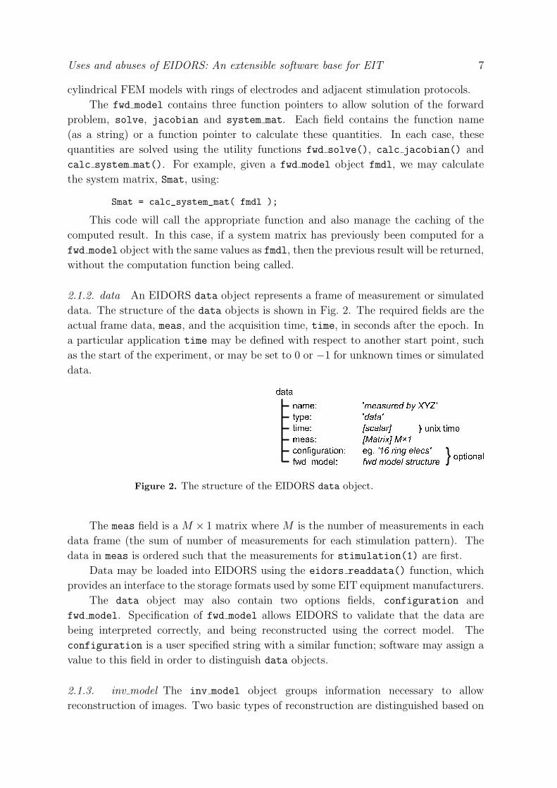
2.1.3. inv model The inv model object groups information necessary to allow
reconstruction of images. Two basic types of reconstruction are distinguished based on
Uses and abuses of EIDORS: An extensible software base for EIT 8
Figure 3. The structure of the EIDORS inv model object.
the reconst type field, “difference” (which calculates an image based on the difference
between two data objects) and “static” (which calculates an image based on a single
data object.
The pointer to the solver function is stored as a string or function
pointer in the solve field. The provided functions are based on regularized
image reconstruction algorithms, and require an image prior and a choice of
hyperparameter. The latter is specified in the hyperparameter field. For
simple cases, a scalar value is provided in the value field. However, for more
complex cases, a hyperparameter selection strategy is specified as a function in
the func field. One example is the noise figure strategy of [1]. This strategy
may be specified by setting hyperparameter.func=’aa calc noise figure’ and
hyperparameter.noise figure=Value.
Image priors are commonly used in two ways, using either a regularization term of
‖λRx‖ or ‖λx‖R, where x is the vector of image element values. In the most common
case, a quadratic norm is used, and these regularization terms may be expressed as
λ2xtRx or λ2xtRtRx, respectively. One implementation concern is to make it clear
to the user which type of image prior is required. EIDORS addresses this by defining
two different functions to calculate image priors, R prior and RtR prior. A user may
provide a value for either or both. When the algorithm specified in the solve field is
called, it will request either an R prior or RtR prior. If the RtR prior is required, but
the R prior is specified, then it will be calculated from RtR. Similarly, EIDORS will
attempt to calculate R from the Cholesky factorization of the RtR prior, if required.
Parameters to an image prior function are specified in a field, using the name of the
image prior function, added to the inv model object.
2.1.4. image The EIDORS image object expresses the reconstructed or simulated
conductivity values. The field elem data (N × 1) is the value of each of the image
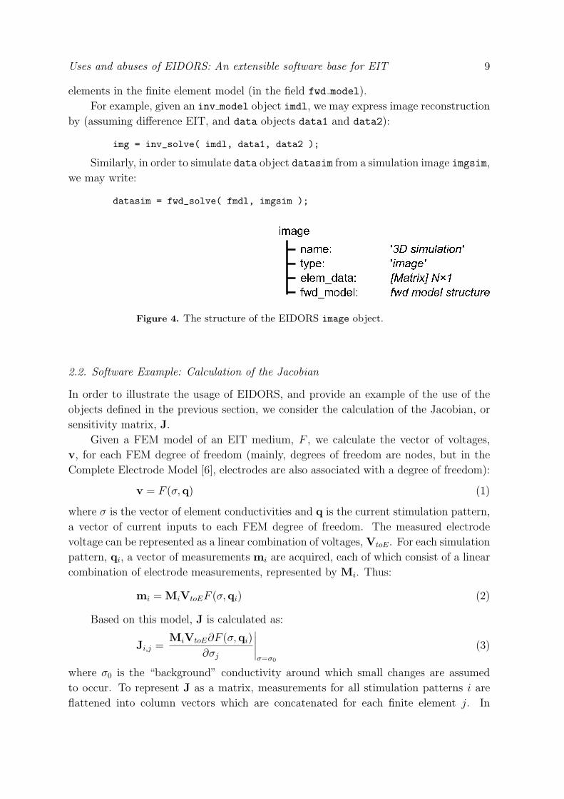
Uses and abuses of EIDORS: An extensible software base for EIT 9
elements in the finite element model (in the field fwd model).
For example, given an inv model object imdl, we may express image reconstruction
by (assuming difference EIT, and data objects data1 and data2):
img = inv_solve( imdl, data1, data2 );
Similarly, in order to simulate data object datasim from a simulation image imgsim,
we may write:
datasim = fwd_solve( fmdl, imgsim );
Figure 4. The structure of the EIDORS image object.
2.2. Software Example: Calculation of the Jacobian
In order to illustrate the usage of EIDORS, and provide an example of the use of the
objects defined in the previous section, we consider the calculation of the Jacobian, or
sensitivity matrix, J.
Given a FEM model of an EIT medium, F , we calculate the vector of voltages,
v, for each FEM degree of freedom (mainly, degrees of freedom are nodes, but in the
Complete Electrode Model [6], electrodes are also associated with a degree of freedom):
v = F (σ,q) (1)
where σ is the vector of element conductivities and q is the current stimulation pattern,
a vector of current inputs to each FEM degree of freedom. The measured electrode
voltage can be represented as a linear combination of voltages, VtoE. For each simulation
pattern, qi, a vector of measurements mi are acquired, each of which consist of a linear
combination of electrode measurements, represented by Mi. Thus:
mi = MiVtoEF (σ,qi) (2)
Based on this model, J is calculated as:
Ji,j =MiVtoE∂F (σ,qi)
∂σj
∣∣∣∣∣σ=σ0
(3)
where σ0 is the “background” conductivity around which small changes are assumed
to occur. To represent J as a matrix, measurements for all stimulation patterns i are
flattened into column vectors which are concatenated for each finite element j. In
Uses and abuses of EIDORS: An extensible software base for EIT 10
EIDORS, the Jacobian is calculated using the function calc jacobian, which takes as
parameters the FEM model (type fwd model) and the image of σ0 (type image).
Objects may be created using the eidors obj() function, which can fill in default
attributes, and keeps track of cached properties. For example, given a fwd model,
fem, and a homogeneous background image of conductivity one, img bkgnd, may be
computed by:
img_bkgnd = eidors_obj(’image’, ’homog bkgnd’);img_bkgnd.elem_data = ones( length(fem.elems) ,1);img_bkgnd.fwd_model = fem;
In this expression, the type field is assigned to ’image’ and then name is assigned
(arbitrarily) to ’homog bkgnd’.
In order to calculate the Jacobian, we call
J= calc_jacobian( fem, img_bkgnd )
which, first, tests to see whether J has been previously calculated for fem and
img bkgnd. If so, the cached value is returned; otherwise, it loads and calls the function
in fem.jacobian, which may be np calc jacobian, which calls the function from the
software of [11]; the returned value is then stored in the cache and returned to the calling
function.
3. Usage Examples
In this section two examples of the usage of EIDORS software functions are provided.
The first illustrates how a change in the electrode configuration and stimulation pattern
can be done with a modification of the fwd model. The second illustrates how to modify
the image reconstruction behaviour of an existing algorithm to add new features.
3.1. Modification of electrode configuration
In this section we wish to explore 3D EIT reconstructions using a sixteen electrode EIT
system. This is a practical problem in many applications where a sixteen electrode EIT
hardware system is available, and the goal is to choose where to put those electrodes to
image a specific physiological process.
In our tests, we use a “zigzag” electrode placement using 16 electrodes, in which
odd and even numbered electrodes are vertically separated onto two different planes (as
illustrated in fig. 6). To illustrate the construction of this model, we begin with the
demonstration finite element configuration given in EIDORS3D [11], which uses two
vertically separated rings of 16 electrodes. applicable to this case.
In order to simulate data, a FEM model object mdl 3d and a conductivity image
need to be created. EIDORS provides a utility function mk common model to provide
many of useful 2D and 3D models. This function may be used as follows to construct
the FEM and use it to simulate voltage patterns.
Uses and abuses of EIDORS: An extensible software base for EIT 11
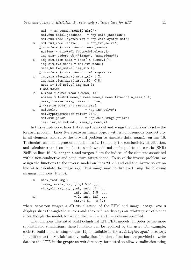
mdl = mk_common_model(’n3r2’);mdl.fwd_model.jacobian = ’np_calc_jacobian’;mdl.fwd_model.system_mat = ’np_calc_system_mat’;
04 mdl.fwd_model.solve = ’np_fwd_solve’;% simulate forward data - homogeneous
n_elems = size(mdl.fwd_model.elems,1);img_sim= eidors_obj(’image’, ’name:demo’);
08 img_sim.elem_data = ones( n_elems,1 );img_sim.fwd_model = mdl.fwd_model;meas_h= fwd_solve( img_sim );% simulate forward data - inhomogeneous
12 img_sim.elem_data(target_A)= 1.2;img_sim.elem_data(target_B)= 0.8;meas_i= fwd_solve( img_sim );% add noise
16 n_meas = size( meas_h.meas, 1);noise= 0.1*std( meas_h.meas-meas_i.meas )*randn( n_meas,1 );meas_i.meas= meas_i.meas + noise;% inverse model and reconstruct
20 mdl.solve = ’np_inv_solve’;mdl.hyperparameter.value= 1e-2;mdl.RtR_prior = ’np_calc_image_prior’;img= inv_solve( mdl, meas_h, meas_i);
In this sample code, lines 1–4 set up the model and assign the functions to solve the
forward problem. Lines 6–9 create an image object with a homogeneous conductivity
in all elements, and solve the forward problem to simulate data, meas h, on line 10.
To simulate an inhomogeneous model, lines 12–13 modify the conductivity distribution,
and calculate meas i on line 14, to which we add noise of signal to noise ratio (SNR)
20dB on lines 16–18. target A and target B are the indices of the elements associated
with a non-conductive and conductive target shape. To solve the inverse problem, we
assign the functions to the inverse model on lines 20–23, and call the inverse solver on
line 24 to calculate the image img. This image may be displayed using the following
imaging functions (Fig. 5):
24 show_fem( img )image_levels(img, [.5,1.5,2.5]);show_slices(img, [inf, inf, .5; ...
inf, inf, 2.5; ...28 -.2, inf, inf; ...
inf,-1.5, 2 ]);
where show fem images a 3D visualization of the FEM and image, image levels
displays slices through the z−axis and show slices displays an arbitrary set of planar
slices though the model, for which the x−, y− and z − axes are specified.
The functions illustrated build cylindrical EIT FEM models. In order to use more
sophisticated simulations, these functions can be replaced by the user. For example,
code to build models using netgen [15] is available in the meshing/netgen/ directory.
In addition to the Matlab based visualization functions, functions are provided to write
data to the VTK in the graphics vtk directory, formatted to allow visualization using
Uses and abuses of EIDORS: An extensible software base for EIT 12
−0.2 0 0.2−0.20
0.20
0.2
0.4
0.6
0.8
1
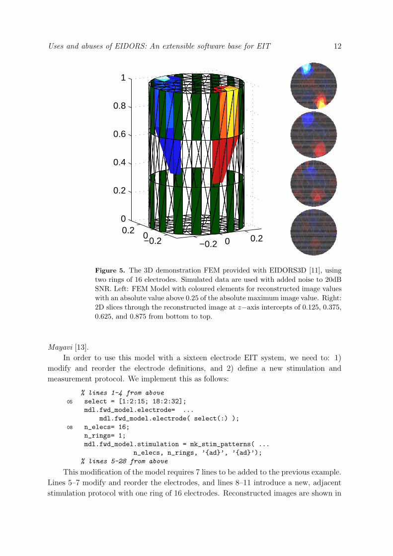
Figure 5. The 3D demonstration FEM provided with EIDORS3D [11], usingtwo rings of 16 electrodes. Simulated data are used with added noise to 20dBSNR. Left: FEM Model with coloured elements for reconstructed image valueswith an absolute value above 0.25 of the absolute maximum image value. Right:2D slices through the reconstructed image at z−axis intercepts of 0.125, 0.375,0.625, and 0.875 from bottom to top.
Mayavi [13].
In order to use this model with a sixteen electrode EIT system, we need to: 1)
modify and reorder the electrode definitions, and 2) define a new stimulation and
measurement protocol. We implement this as follows:
% lines 1-4 from above
05 select = [1:2:15; 18:2:32];mdl.fwd_model.electrode= ...
mdl.fwd_model.electrode( select(:) );08 n_elecs= 16;
n_rings= 1;mdl.fwd_model.stimulation = mk_stim_patterns( ...
n_elecs, n_rings, ’{ad}’, ’{ad}’);% lines 5-28 from above
This modification of the model requires 7 lines to be added to the previous example.
Lines 5–7 modify and reorder the electrodes, and lines 8–11 introduce a new, adjacent
stimulation protocol with one ring of 16 electrodes. Reconstructed images are shown in
Uses and abuses of EIDORS: An extensible software base for EIT 13
−0.2 0 0.2−0.20
0.20
0.2
0.4
0.6
0.8
1
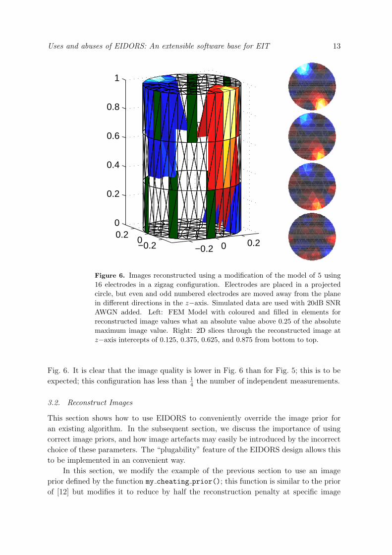
Figure 6. Images reconstructed using a modification of the model of 5 using16 electrodes in a zigzag configuration. Electrodes are placed in a projectedcircle, but even and odd numbered electrodes are moved away from the planein different directions in the z−axis. Simulated data are used with 20dB SNRAWGN added. Left: FEM Model with coloured and filled in elements forreconstructed image values what an absolute value above 0.25 of the absolutemaximum image value. Right: 2D slices through the reconstructed image atz−axis intercepts of 0.125, 0.375, 0.625, and 0.875 from bottom to top.
Fig. 6. It is clear that the image quality is lower in Fig. 6 than for Fig. 5; this is to be
expected; this configuration has less than 14
the number of independent measurements.
3.2. Reconstruct Images
This section shows how to use EIDORS to conveniently override the image prior for
an existing algorithm. In the subsequent section, we discuss the importance of using
correct image priors, and how image artefacts may easily be introduced by the incorrect
choice of these parameters. The “plugability” feature of the EIDORS design allows this
to be implemented in an convenient way.
In this section, we modify the example of the previous section to use an image
prior defined by the function my cheating prior(); this function is similar to the prior
of [12] but modifies it to reduce by half the reconstruction penalty at specific image
Uses and abuses of EIDORS: An extensible software base for EIT 14
elements chosen by the user. To do this, we replace line 22 from the previous example.
% lines 1-21 from above
mdl.RtR_prior.func = ’my_cheating_prior’;mdl.my_cheating_prior.target = [target_A];
% lines 23-28 from above
We define the function my cheating prior in a separate file:
function Reg = my_cheating_prior( inv_model );inv_model.RtR_prior.func = ’np_calc_image_prior’;Reg= calc_image_prior( inv_model );
04 % modify Reg matrix
posn = inv_model.my_cheating_prior.target;posn = posn + (posn-1)*size(Reg,1);Reg(posn) = Reg(posn) * 0.5;
In lines 2–3, the previous prior function is calculated from np calc image prior().
Subsequently, on lines 5–7, the position of target elements is calculated and the penalty
term multiplied by 0.5. Line 6 calculates a column major index into the matrix Reg of
the diagonal element indicated by posn. As expected, images reconstructed with this
prior show sharper images than that of 6. The implications of this type of “cheating”
are explored in detail in the following section.
4. Cheating with EIT
One general issue with inverse problem software is the difficulty of correctly
implementing algorithms, and the consequent ease with which subtle numerical bugs
can be inadvertently introduced. EIDORS helps with this issue, by allowing sharing and
reuse of well documented and debugged software. On the other hand, since EIDORS is
designed to facilitate use by non-specialists, it may inadvertently encourage numerical
errors. In order to address this issue, we develop in this section a list of ways in which
such errors, or “cheats” may occur. Our hope is that such a list will assist authors of
software to avoid such implemention issues.
4.1. Sample Problem: The “happy” transform
In this section, we describe some simple implementation errors that may occur with
common, linear regularization algorithms. As the solution strategy becomes more
complex, such as for non-linear and iterative imaging algorithms, there are more complex
interactions between different parts of the algorithms, leading to more possibilities for
“cheating”.
To motivate the problem, assume that EIT measurement data have been acquired
from a 2D simulated phantom which resembles a sad face. Being of an optimistic outlook,
we wish that the reconstructed images represent a happy face instead. Fig. 7 illustrates
what we will refer to as the “happy transform”. We choose this example because it is
important to distinguish two types of reconstruction artefacts. Most artefacts result in
adding noise to images. While such noise is inconvenient, it does not cause a strong
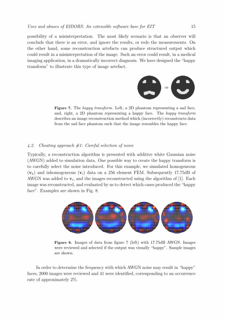
Uses and abuses of EIDORS: An extensible software base for EIT 15
possibility of a misinterpretation. The most likely scenario is that an observer will
conclude that there is an error, and ignore the results, or redo the measurements. On
the other hand, some reconstruction artefacts can produce structured output which
could result in a misinterpretation of the image. Such an error could result, in a medical
imaging application, in a dramatically incorrect diagnosis. We have designed the “happy
transform” to illustrate this type of image artefact.
⇒
Figure 7. The happy transform. Left, a 2D phantom representing a sad face,and, right, a 2D phantom representing a happy face. The happy transformdescribes an image reconstruction method which (incorrectly) reconstructs datafrom the sad face phantom such that the image resembles the happy face.
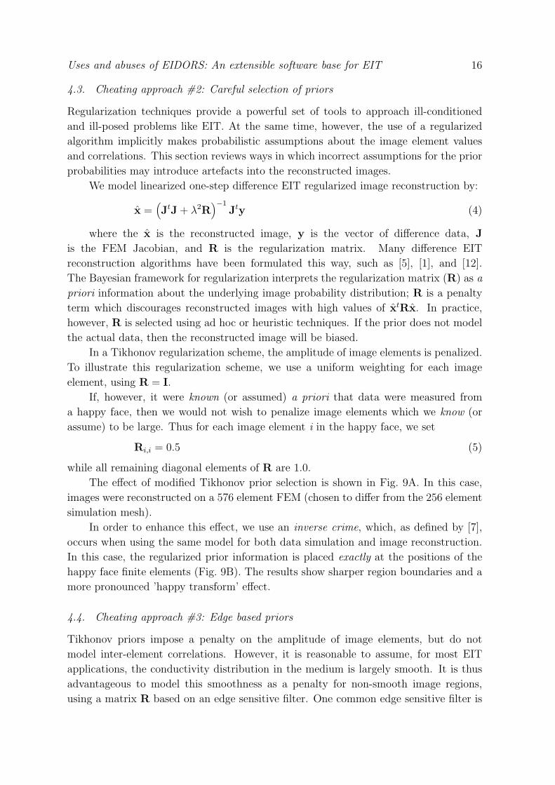
4.2. Cheating approach #1: Careful selection of noise
Typically, a reconstruction algorithm is presented with additive white Gaussian noise
(AWGN) added to simulation data. One possible way to create the happy transform is
to carefully select the noise introduced. For this example, we simulated homogeneous
(vh) and inhomogeneous (vi) data on a 256 element FEM. Subsequently 17.75dB of
AWGN was added to vi, and the images reconstructed using the algorithm of [1]. Each
image was reconstructed, and evaluated by us to detect which cases produced the “happy
face”. Examples are shown in Fig. 8.
Figure 8. Images of data from figure 7 (left) with 17.75dB AWGN. Imageswere reviewed and selected if the output was visually “happy”. Sample imagesare shown.
In order to determine the frequency with which AWGN noise may result in “happy”
faces, 2000 images were reviewed and 41 were identified, corresponding to an occurrence
rate of approximately 2%.
Uses and abuses of EIDORS: An extensible software base for EIT 16
4.3. Cheating approach #2: Careful selection of priors
Regularization techniques provide a powerful set of tools to approach ill-conditioned
and ill-posed problems like EIT. At the same time, however, the use of a regularized
algorithm implicitly makes probabilistic assumptions about the image element values
and correlations. This section reviews ways in which incorrect assumptions for the prior
probabilities may introduce artefacts into the reconstructed images.
We model linearized one-step difference EIT regularized image reconstruction by:
x =(JtJ + λ2R
)−1Jty (4)
where the x is the reconstructed image, y is the vector of difference data, J
is the FEM Jacobian, and R is the regularization matrix. Many difference EIT
reconstruction algorithms have been formulated this way, such as [5], [1], and [12].
The Bayesian framework for regularization interprets the regularization matrix (R) as a
priori information about the underlying image probability distribution; R is a penalty
term which discourages reconstructed images with high values of xtRx. In practice,
however, R is selected using ad hoc or heuristic techniques. If the prior does not model
the actual data, then the reconstructed image will be biased.
In a Tikhonov regularization scheme, the amplitude of image elements is penalized.
To illustrate this regularization scheme, we use a uniform weighting for each image
element, using R = I.
If, however, it were known (or assumed) a priori that data were measured from
a happy face, then we would not wish to penalize image elements which we know (or
assume) to be large. Thus for each image element i in the happy face, we set
Ri,i = 0.5 (5)
while all remaining diagonal elements of R are 1.0.
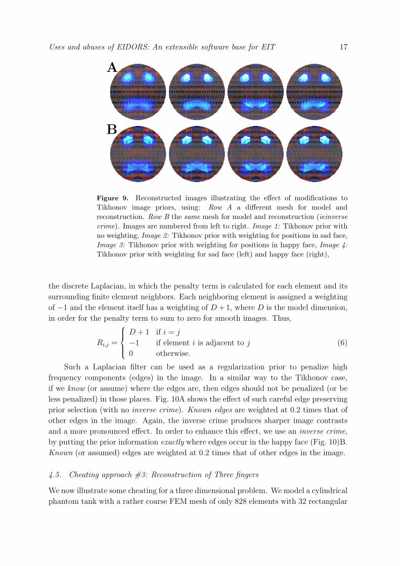
The effect of modified Tikhonov prior selection is shown in Fig. 9A. In this case,
images were reconstructed on a 576 element FEM (chosen to differ from the 256 element
simulation mesh).
In order to enhance this effect, we use an inverse crime, which, as defined by [7],
occurs when using the same model for both data simulation and image reconstruction.
In this case, the regularized prior information is placed exactly at the positions of the
happy face finite elements (Fig. 9B). The results show sharper region boundaries and a
more pronounced ’happy transform’ effect.
4.4. Cheating approach #3: Edge based priors
Tikhonov priors impose a penalty on the amplitude of image elements, but do not
model inter-element correlations. However, it is reasonable to assume, for most EIT
applications, the conductivity distribution in the medium is largely smooth. It is thus
advantageous to model this smoothness as a penalty for non-smooth image regions,
using a matrix R based on an edge sensitive filter. One common edge sensitive filter is
Uses and abuses of EIDORS: An extensible software base for EIT 17
A
B
Figure 9. Reconstructed images illustrating the effect of modifications toTikhonov image priors, using: Row A a different mesh for model andreconstruction. Row B the same mesh for model and reconstruction (ieinversecrime). Images are numbered from left to right. Image 1: Tikhonov prior withno weighting, Image 2: Tikhonov prior with weighting for positions in sad face,Image 3: Tikhonov prior with weighting for positions in happy face, Image 4:Tikhonov prior with weighting for sad face (left) and happy face (right),
the discrete Laplacian, in which the penalty term is calculated for each element and its
surrounding finite element neighbors. Each neighboring element is assigned a weighting
of −1 and the element itself has a weighting of D + 1, where D is the model dimension,
in order for the penalty term to sum to zero for smooth images. Thus,
Ri,j =
D + 1 if i = j
−1 if element i is adjacent to j
0 otherwise.
(6)
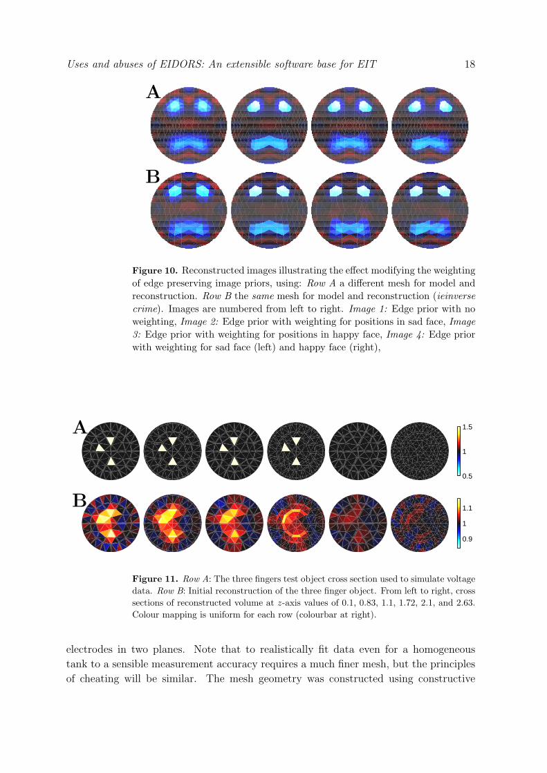
Such a Laplacian filter can be used as a regularization prior to penalize high
frequency components (edges) in the image. In a similar way to the Tikhonov case,
if we know (or assume) where the edges are, then edges should not be penalized (or be
less penalized) in those places. Fig. 10A shows the effect of such careful edge preserving
prior selection (with no inverse crime). Known edges are weighted at 0.2 times that of
other edges in the image. Again, the inverse crime produces sharper image contrasts
and a more pronounced effect. In order to enhance this effect, we use an inverse crime,
by putting the prior information exactly where edges occur in the happy face (Fig. 10)B.
Known (or assumed) edges are weighted at 0.2 times that of other edges in the image.
4.5. Cheating approach #3: Reconstruction of Three fingers
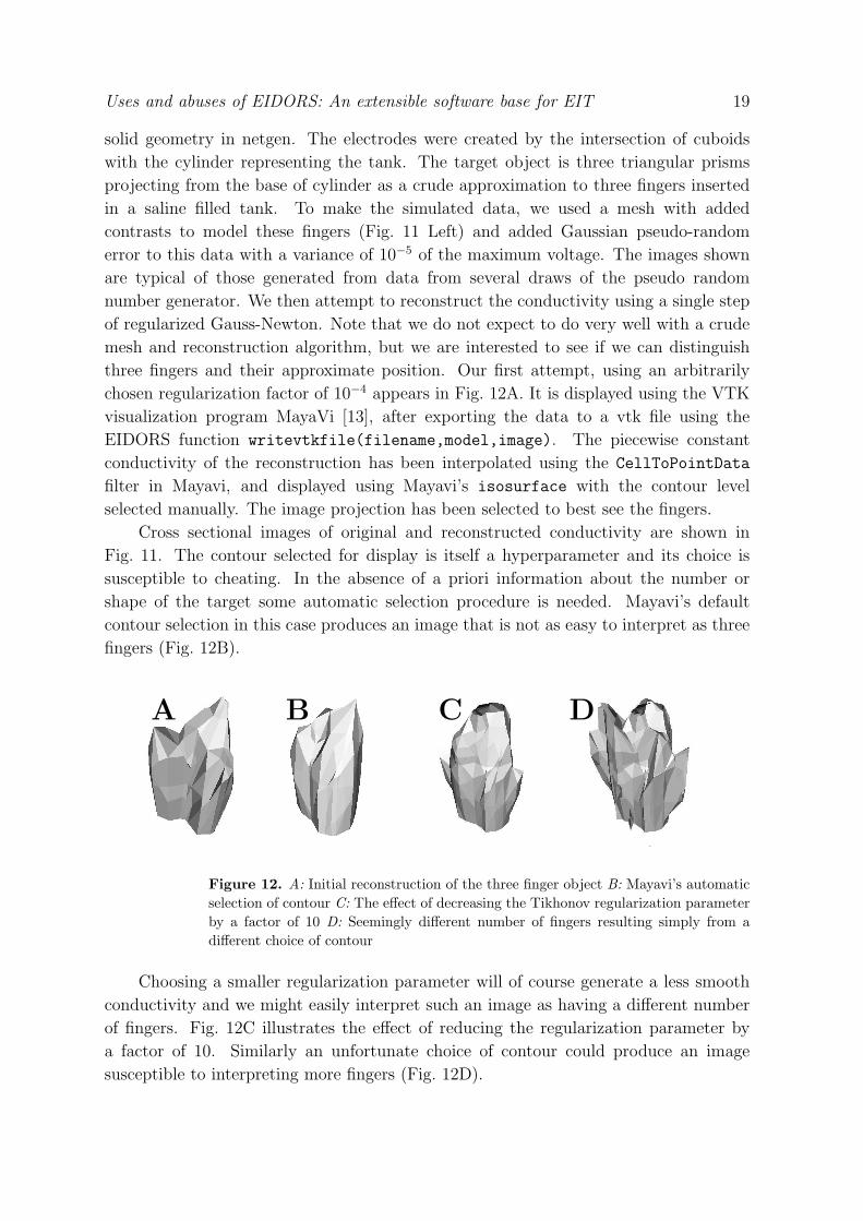
We now illustrate some cheating for a three dimensional problem. We model a cylindrical
phantom tank with a rather coarse FEM mesh of only 828 elements with 32 rectangular
Uses and abuses of EIDORS: An extensible software base for EIT 18
A
B
Figure 10. Reconstructed images illustrating the effect modifying the weightingof edge preserving image priors, using: Row A a different mesh for model andreconstruction. Row B the same mesh for model and reconstruction (ieinversecrime). Images are numbered from left to right. Image 1: Edge prior with noweighting, Image 2: Edge prior with weighting for positions in sad face, Image3: Edge prior with weighting for positions in happy face, Image 4: Edge priorwith weighting for sad face (left) and happy face (right),
0.5
1
1.5
0.9
1
1.1
A
B
Figure 11. Row A: The three fingers test object cross section used to simulate voltagedata. Row B: Initial reconstruction of the three finger object. From left to right, crosssections of reconstructed volume at z-axis values of 0.1, 0.83, 1.1, 1.72, 2.1, and 2.63.Colour mapping is uniform for each row (colourbar at right).
electrodes in two planes. Note that to realistically fit data even for a homogeneous
tank to a sensible measurement accuracy requires a much finer mesh, but the principles
of cheating will be similar. The mesh geometry was constructed using constructive
Uses and abuses of EIDORS: An extensible software base for EIT 19
solid geometry in netgen. The electrodes were created by the intersection of cuboids
with the cylinder representing the tank. The target object is three triangular prisms
projecting from the base of cylinder as a crude approximation to three fingers inserted
in a saline filled tank. To make the simulated data, we used a mesh with added
contrasts to model these fingers (Fig. 11 Left) and added Gaussian pseudo-random
error to this data with a variance of 10−5 of the maximum voltage. The images shown
are typical of those generated from data from several draws of the pseudo random
number generator. We then attempt to reconstruct the conductivity using a single step
of regularized Gauss-Newton. Note that we do not expect to do very well with a crude
mesh and reconstruction algorithm, but we are interested to see if we can distinguish
three fingers and their approximate position. Our first attempt, using an arbitrarily
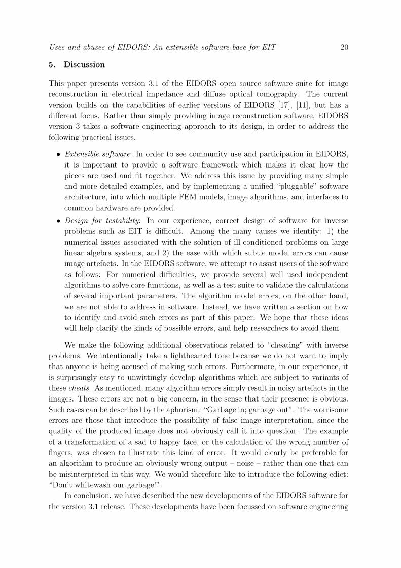
chosen regularization factor of 10−4 appears in Fig. 12A. It is displayed using the VTK
visualization program MayaVi [13], after exporting the data to a vtk file using the
EIDORS function writevtkfile(filename,model,image). The piecewise constant
conductivity of the reconstruction has been interpolated using the CellToPointData
filter in Mayavi, and displayed using Mayavi’s isosurface with the contour level
selected manually. The image projection has been selected to best see the fingers.
Cross sectional images of original and reconstructed conductivity are shown in
Fig. 11. The contour selected for display is itself a hyperparameter and its choice is
susceptible to cheating. In the absence of a priori information about the number or
shape of the target some automatic selection procedure is needed. Mayavi’s default
contour selection in this case produces an image that is not as easy to interpret as three
fingers (Fig. 12B).
A B C D
Figure 12. A: Initial reconstruction of the three finger object B: Mayavi’s automaticselection of contour C: The effect of decreasing the Tikhonov regularization parameterby a factor of 10 D: Seemingly different number of fingers resulting simply from adifferent choice of contour
Choosing a smaller regularization parameter will of course generate a less smooth
conductivity and we might easily interpret such an image as having a different number
of fingers. Fig. 12C illustrates the effect of reducing the regularization parameter by
a factor of 10. Similarly an unfortunate choice of contour could produce an image
susceptible to interpreting more fingers (Fig. 12D).
Uses and abuses of EIDORS: An extensible software base for EIT 20
5. Discussion
This paper presents version 3.1 of the EIDORS open source software suite for image
reconstruction in electrical impedance and diffuse optical tomography. The current
version builds on the capabilities of earlier versions of EIDORS [17], [11], but has a
different focus. Rather than simply providing image reconstruction software, EIDORS
version 3 takes a software engineering approach to its design, in order to address the
following practical issues.
• Extensible software: In order to see community use and participation in EIDORS,
it is important to provide a software framework which makes it clear how the
pieces are used and fit together. We address this issue by providing many simple
and more detailed examples, and by implementing a unified “pluggable” software
architecture, into which multiple FEM models, image algorithms, and interfaces to
common hardware are provided.
• Design for testability: In our experience, correct design of software for inverse
problems such as EIT is difficult. Among the many causes we identify: 1) the
numerical issues associated with the solution of ill-conditioned problems on large
linear algebra systems, and 2) the ease with which subtle model errors can cause
image artefacts. In the EIDORS software, we attempt to assist users of the software
as follows: For numerical difficulties, we provide several well used independent
algorithms to solve core functions, as well as a test suite to validate the calculations
of several important parameters. The algorithm model errors, on the other hand,
we are not able to address in software. Instead, we have written a section on how
to identify and avoid such errors as part of this paper. We hope that these ideas
will help clarify the kinds of possible errors, and help researchers to avoid them.
We make the following additional observations related to “cheating” with inverse
problems. We intentionally take a lighthearted tone because we do not want to imply
that anyone is being accused of making such errors. Furthermore, in our experience, it
is surprisingly easy to unwittingly develop algorithms which are subject to variants of
these cheats. As mentioned, many algorithm errors simply result in noisy artefacts in the
images. These errors are not a big concern, in the sense that their presence is obvious.
Such cases can be described by the aphorism: “Garbage in; garbage out”. The worrisome
errors are those that introduce the possibility of false image interpretation, since the
quality of the produced image does not obviously call it into question. The example
of a transformation of a sad to happy face, or the calculation of the wrong number of
fingers, was chosen to illustrate this kind of error. It would clearly be preferable for
an algorithm to produce an obviously wrong output – noise – rather than one that can
be misinterpreted in this way. We would therefore like to introduce the following edict:
“Don’t whitewash our garbage!”.
In conclusion, we have described the new developments of the EIDORS software for
the version 3.1 release. These developments have been focussed on software engineering
Uses and abuses of EIDORS: An extensible software base for EIT 21
improvements that will facilitate collaborative use, modification and enhancement of the
software by the EIT community. Open source software like EIDORS could potentially
be a dramatical help to research and development in medical imaging fields like EIT. We
are hopeful that EIDORS will assist in the development and testing of new approaches
and ideas, and will ease the use of advanced algorithms in experimental, industrial and
clinical applications of these technologies.
References
[1] Adler A and Guardo R 1996 Electrical impedance tomography: regularised imaging and contrastdetection IEEE Trans. Med. Imaging 15 170–9
[2] Asfaw Y and Adler A 2005 Automatic detection of detached and erroneous electrodes in electricalimpedance tomography Physiol. Meas., 26 S175–S183
[3] Borsic A 2002 Regularisation Methods for Imaging from Electrical Measurements PhD thesis,Oxford Brookes University, U.K.,
[4] Cederqvist P 2002 Version Management with CVS, Network Theory Ltd, Bristol, UK[5] Cheney M Isaacson D Newell J C Simske C and Goble J C 1990 NOSER: An algorithm for solving
the inverse conductivity problem Int. J. Imaging Systems & Technol. 2 66–75[6] Cheng K-S Isaacson D Newell J C and Gisser D G 1989 Electrode models for electric current
computed tomography IEEE Trans Biomed Eng 36 918–924[7] Colton D and Kress R 1992 Inverse Acoustic and Electromagnetic Scattering Theory Springer,
Berlin.[8] Eaton J W 2002 Gnu Octave Manual Network Theory Ltd, Bristol, UK[9] Free Software Foundation 1991 GNU General Public Licence Boston MA USA
http://www.gnu.org/copyleft/gpl.html
[10] Gamma E Helm R Johnson R and Vlissides J 1995 Design Patterns: Elements of Reusable Object-Oriented Software Addison-Wesley, Boston, MA, USA
[11] Polydorides N and Lionheart W R B 2002 A Matlab toolkit for three-dimensional electricalimpedance tomography: a contribution to the Electrical Impedance and Diffuse OpticalReconstruction Software project, Meas. Sci. Technol. 13 1871–1883
[12] Polydorides N 2002 Image reconstruction algorithms for soft-field tomography Ph.D. Thesis,University of Manchester Institute of Science and Technology, U.K.
[13] Ramachandran P 2003 Scientific data visualization with MayaVi Conf. SciPy: Python for ScientificComputing Pasadena, CA, USA http://mayavi.sf.net/
[14] Soleimani M Gomez-Laberge C and Adler A 2005 Imaging of conductivity changes and electrodemovement in EIT Physiol. Meas., submitted
[15] Schoberl J 1997 NETGEN - An advancing front 2D/3D-mesh generator based on abstract rules.Comput. Visual. Sci 1 41–52 http://www.hpfem.jku.at/netgen/
[16] Vauhkonen M 1997 Electrical impedance tomography and prior information PhD thesis, Universityof Kuopio, Finland
[17] Vauhkonen M, Lionheart W R B, Heikkinen L M, Vauhkonen P J and Kaipio J P, 2000 A MATLABpackage for the EIDORS project to reconstruct two-dimensional EIT images Physiol. Meas. 22107–111