Inferring the Ancestral Origin of Sockeye Salmon,

Oncorhynchus nerka, in The Lake Washington

Basin: A Statistical Method in

Theory and Application

by

Eric C. Anderson

A thesis submitted in partial fulfillment

of the requirements for the degree of

Master of Science

University of Washington

1998

Approved by

(Chairperson of Supervisory Committee)

Program Authorized

to O!er Degree

Date

In presenting this thesis in partial fulfillment of the requirements for a Master’s de-

gree at the University of Washington, I agree that the Library shall make its copies

freely available for inspection. I further agree that extensive copying of this thesis is

allowable only for scholarly purposes, consistent with “fair use” as prescribed in the

U.S. Copyright Law. Any other reproduction for any purposes or by any means shall

not be allowed without my permission.

Signature

Date

University of Washington

Abstract

Inferring the Ancestral Origin of Sockeye Salmon,

Oncorhynchus nerka, in The Lake Washington

Basin: A Statistical Method in

Theory and Application

by Eric C. Anderson

Chairperson of Supervisory Committee: Associate Professor Thomas Sibley

School of Fisheries

It was once held that any native populations of anadromous sockeye salmon in the

Lake Washington Basin were extirpated by the changes in the lake following the

completion of the Lake Washington Ship Canal in the early 1900’s, and were replaced

by sockeye planted from Baker or Cultus lakes in the 1930’s and 1940’s. The authors

of two surveys of neutral genetic markers in Lake Washington sockeye populations,

however, suggest that the sockeye spawning in Bear Creek and its tributaries are of

native origin. I argue that one cannot prove that the fish in Bear Creek are of native

origin, but it may be possible to statistically exclude the possibility that sockeye in

Bear Creek derive exclusively from Baker Lake or Cultus Lake. I present a likelihood

ratio test of the hypothesis that Bear Creek fish could have derived exclusively from

Baker (or Cultus) Lake against the alternative hypothesis that at least some of the

ancestry of the Bear Creek population must be from a source other than Baker (or

Cultus) lake. The test is based on a probability model which includes uncertainty in

the data due both to sampling error and to the error due to random genetic drift.

Several di!erent formulations and approximations are used to compute the likeli-

hood ratio as appropriate for four di!erent loci on which data are available.

The method requires independent knowledge of the historical e!ective sizes of the

populations in Bear Creek, Cultus Lake, and Baker Lake. I perform simulations based

on very good historical data suggesting that a lower bound on e!ective size for the

Baker Lake population is about 250 individuals and for the Cultus Lake population

is about 800. Early run-size data for Bear Creek are not available, so I perform

simulations based on a reasonable scenario that show how the Bear Creek population

might have grown from the early 1940’s so as to have an e!ective size of 100. If these

numbers for e!ective size are accurate, it is unlikely that the sockeye inhabiting Bear

Creek could have descended exclusively from fish introduced from either Baker Lake

or Cultus Lake. Unfortunately, this result depends highly on the assumed run sizes

in Bear Creek in years with little or no data.

TABLE OF CONTENTS

List of Figures iv

List of Tables vi

Chapter 1: Introduction 1

1.1 Overview and Objectives of the Thesis . . . . . . . . . . . . . . . . . 1

1.2 General Introduction to Lake Washington . . . . . . . . . . . . . . . 2

1.3 History of O. nerka in the Lake Washington Basin . . . . . . . . . . . 4

1.4 Recent Genetic Work in Lake Washington . . . . . . . . . . . . . . . 7

Chapter 2: The Statistical Framework for Hypothesis Testing 12

2.1 Testable Hypotheses . . . . . . . . . . . . . . . . . . . . . . . . . . . 12

2.2 The Probability Model . . . . . . . . . . . . . . . . . . . . . . . . . . 14

2.3 The Likelihood-Ratio Test . . . . . . . . . . . . . . . . . . . . . . . . 18

2.4 Genetic Drift and E!ective Population Number . . . . . . . . . . . . 20

2.5 t-Step Transition Probabilities in the Wright-Fisher Model . . . . . . 23

2.5.1 Drift as a Markov Process . . . . . . . . . . . . . . . . . . . . 24

2.5.2 Di!usion Approximations to Genetic Drift . . . . . . . . . . . 27

2.5.3 Brownian Motion and Stereographic Projection . . . . . . . . 27

2.5.4 Other Approximations to Drift Probabilities . . . . . . . . . . 34

2.6 Assessing the Approximations . . . . . . . . . . . . . . . . . . . . . . 35

2.7 Adding the Sampling Step . . . . . . . . . . . . . . . . . . . . . . . . 42

2.7.1 Sample mass methods . . . . . . . . . . . . . . . . . . . . . . 42

2.7.2 Sample Density Methods . . . . . . . . . . . . . . . . . . . . . 44

2.8 Sampling with Recessive or “Null” Alleles . . . . . . . . . . . . . . . 46

2.8.1 A Sample Density Method for Null Alleles . . . . . . . . . . . 47

2.9 The Distribution of the Test Statistic . . . . . . . . . . . . . . . . . . 49

2.10 Review of Assumptions . . . . . . . . . . . . . . . . . . . . . . . . . . 54

Chapter 3: The Statistical Method in Practice 56

3.1 Data for Baker and Cultus Lakes and Bear Creek . . . . . . . . . . . 56

3.2 Determining E!ective Sizes of the Populations . . . . . . . . . . . . . 58

3.2.1 Baker Lake Simulations . . . . . . . . . . . . . . . . . . . . . 60

3.2.2 Simulations for Cultus Lake . . . . . . . . . . . . . . . . . . . 63

3.2.3 Simulations for Bear Creek . . . . . . . . . . . . . . . . . . . . 66

3.2.4 On the shapes of the distributions . . . . . . . . . . . . . . . . 70

3.3 Computing Likelihood Ratios for HA . . . . . . . . . . . . . . . . . . 70

3.4 Computing Likelihood Ratios for HC . . . . . . . . . . . . . . . . . . 73

3.5 Testing the Cedar River . . . . . . . . . . . . . . . . . . . . . . . . . 74

3.6 Results of the Likelihood Ratio Tests . . . . . . . . . . . . . . . . . . 77

3.6.1 Result for HA . . . . . . . . . . . . . . . . . . . . . . . . . . . 77

3.6.2 Result for HC . . . . . . . . . . . . . . . . . . . . . . . . . . . 78

3.6.3 Result for HR: Making sure this test doesn’t reject everything 80

3.7 Discussion . . . . . . . . . . . . . . . . . . . . . . . . . . . . . . . . . 82

3.7.1 The test and other applications . . . . . . . . . . . . . . . . . 82

3.7.2 Interpretation of p-values . . . . . . . . . . . . . . . . . . . . . 85

3.7.3 Conclusions on Bear Creek . . . . . . . . . . . . . . . . . . . . 88

3.7.4 Future work on Bear Creek . . . . . . . . . . . . . . . . . . . 90

Bibliography 94

ii

Appendix A: Determining the E!ective Sizes 103

A.1 Population Sizes and Age Composition of Cultus Lake Sockeye . . . . 103

A.2 Determining E!ective Size of the Cedar River Population . . . . . . . 103

Appendix B: Routines for Computing the Likelihood Ratio 106

B.1 Diallelic Codominant Loci . . . . . . . . . . . . . . . . . . . . . . . . 106

B.2 Triallelic Codominant Locus . . . . . . . . . . . . . . . . . . . . . . . 107

B.3 Diallelic Locus With Recessive—PGM–1* . . . . . . . . . . . . . . . 109

B.4 Diallelic Locus With Recessive—LDH–A1* . . . . . . . . . . . . . . . 110

iii

LIST OF FIGURES

1.1 Lake Washington drainage basin map . . . . . . . . . . . . . . . . . . 3

1.2 Lake Washington sockeye population sizes . . . . . . . . . . . . . . . 7

1.3 Genetic distances between Lake Washington sockeye populations . . . 9

2.1 Diagram of the probability model . . . . . . . . . . . . . . . . . . . . 16

2.2 The unit circle . . . . . . . . . . . . . . . . . . . . . . . . . . . . . . . 30

2.3 The unit sphere . . . . . . . . . . . . . . . . . . . . . . . . . . . . . . 31

2.4 Projecting a circle into a line . . . . . . . . . . . . . . . . . . . . . . . 33

2.5 Probability distribution after drift from p = .5 . . . . . . . . . . . . . 36

2.6 Probability distribution after drift from p = .2 . . . . . . . . . . . . . 37

2.7 Approximations to the exact probability . . . . . . . . . . . . . . . . 38

2.8 Fixation probabilities . . . . . . . . . . . . . . . . . . . . . . . . . . . 40

2.9 Approximations to the exact probability shifted by ! . . . . . . . . . 40

2.10 Horizontal deviations of the approximations . . . . . . . . . . . . . . 41

2.11 Simulated values of the test statistic I . . . . . . . . . . . . . . . . . . 51

2.12 Simulated values of the test statistic II . . . . . . . . . . . . . . . . . 52

2.13 Cumulative proportion of simulated test statistics . . . . . . . . . . . 53

3.1 Population with overlapping year classes and fluctuating size . . . . . 59

3.2 Baker Lake sockeye run size 1930–1996 . . . . . . . . . . . . . . . . . 61

3.3 E!ective size of the Baker Lake Population . . . . . . . . . . . . . . . 64

3.4 Cultus Lake Escapement 1942–1993 . . . . . . . . . . . . . . . . . . . 65

3.5 Imaginary population sizes for Bear Creek . . . . . . . . . . . . . . . 67

iv

3.6 Overlapping vs Wright-Fisher Populations: transition probabilities . . 71

v

LIST OF TABLES

1.1 Transplants of sockeye salmon to Lake Washington . . . . . . . . . . 6

2.1 Number of allele frequency states . . . . . . . . . . . . . . . . . . . . 26

3.1 Data from Hendry et al. (1996) . . . . . . . . . . . . . . . . . . . . 57

3.2 Early Bear Creek run sizes—an example scenario . . . . . . . . . . . 69

3.3 Data from Hendry et al. (1996) for the Cedar River . . . . . . . . . 76

3.4 " for HA at di!erent e!ective sizes . . . . . . . . . . . . . . . . . . . 79

3.5 " for HC at di!erent e!ective sizes . . . . . . . . . . . . . . . . . . . 80

3.6 " for HR at di!erent e!ective sizes . . . . . . . . . . . . . . . . . . . 81

A.1 Escapement of Cultus Lake Sockeye . . . . . . . . . . . . . . . . . . . 103

A.2 Cedar River Escapements used in the Simulations . . . . . . . . . . . 105

vi

ACKNOWLEDGMENTS

I wish to express my sincere gratitude to the members of my Supervisory com-

mittee, Dr. Chris Foote, Dr. Paul Bentzen, and chair, Dr. Thomas Sibley. This thesis

developed out of a nagging concern I had regarding the proper statistical treatment

of some molecular genetic data I had planned to collect. As it turned out, devising

an appropriate statistical method was a substantial problem in and of itself, and I

especially thank Dr. Sibley for recognizing which areas of research most excited me,

and allowing me to pursue them despite the fact that they are somewhat outside of

his areas of research. I am also grateful for the support, kindness, and insight of Dr.

Fred Utter.

Dr. Joseph Felsenstein of the Department of Genetics generously o!ered me two

quarters of tutorial study in population genetics. Without this I may never have

gotten started on this path I so thoroughly enjoy. He also introduced me to the

method of maximum likelihood, and, perhaps more importantly, he introduced me

to Dr. Elizabeth Thompson in the Department of Statistics. She has helped me a

great deal with this thesis and was an excellent and supportive instructor of Statistics

512 and 513; the content of those courses figures heavily in the pages that follow. I

am extremely fortunate to be currently undertaking my dissertation in the QERM

program under her guidance.

Andrew Hendry, whose work inspired this thesis has been kind about providing

data and information. He has also been consistently supportive of my work, has

provided hours of insightful discussion, and contributed a great deal of help in the

preparation of this thesis.

vii

I also thank members of the Washington Department of Fish and Wildlife: Gary

Sprague for the Baker Lake population size data, Bob Pfei!er for various ideas and

discussion, and Ron Egan for Lake Washington escapement data. Mike LaPointe at

the Pacific Salmon Commission provided population data from Cultus Lake. Indi-

viduals at the National Marine Fisheries Service were also extremely helpful: Robin

Waples answered many questions and Rick Gustafson shared much hard won infor-

mation regarding the history of sockeye salmon in Washington.

The Mathematical Biology Group at the Department of Zoology provided (always)

lively comments on this work throughout its development. Similarly I appreciate the

insightful comments of the students in Dr. Thompson’s “Computational Population

Genetics” lab-group meetings.

I began my graduate work at the School of Fisheries with Dr. Robert Naiman. My

research interests strayed from his, but I thank him for being supportive throughout

in seeing that I received the most of what I wanted from my time at the UW.

Outside of the academic world, I owe much to the extended “Sunnyside House”

crew—my support gang of friends. They know who they are. And finally, special

thanks to two men from whom I’ve learned a lot about both mathematics and moun-

tains. Recently Dr. Karel Zikan, a friend, housemate, and mathematician whose

generous assessments of my mathematical abilities encouraged me to delve back into

quantitative realms. And John Rosendahl, a friend and mentor from my teen years—I

still have vivid memories from my junior year in high school, of riding in his old VW

van to various rock-climbing destinations discussing Taylor Series or Markov chains,

etc. I think of him whenever I do mathematical things.

I acknowledge the generous financial support of the School of Fisheries’ H. Mason

Keeler Endowment for Excellence fellowship and the National Science Foundation’s

Mathematical Biology Training Grant.

viii

Chapter 1

INTRODUCTION

This thesis investigates, using allele-frequency data in an hypothesis-testing frame-

work, the origin of sockeye salmon, Oncorhynchus nerka, in the Lake Washington

basin. Specifically, I test whether the sockeye population in the Bear Creek drainage

descended, at least in part, from fish other than those introduced from Baker and Cul-

tus Lakes in the 1930’s and 1940’s. Previous authors have inferred that one (Hendry

et al. 1996) or several (Seeb and Wishard 1977) Lake Washington sockeye popu-

lations are of “native” origin, but they have not assessed the probability that their

conclusions are incorrect (Type I error probability) because there is no straightfoward

or “standard” statistical test for doing so. The ability to assign a level of confidence

to one’s inferences regarding the origin of these sockeye populations, and especially of

the Bear Creek population, is desirable in light of recent controversies over hatchery

supplementation in the Cedar River and the designation of Evolutionarily Significant

Units (ESU’s) by the National Marine Fisheries Service (NMFS). Indeed, NMFS

recently declared the sockeye of Bear Creek and its tributaries a “provisional” ESU

(Gustafson et al. 1997).

1.1 Overview and Objectives of the Thesis

There are three chapters of this thesis. This chapter provides an overview, introduces

the physical setting of Lake Washington, reviews the history of sockeye salmon in the

basin and presents the conclusions of previous genetic work. In Chapter 2, I discuss

2

which hypotheses about the origin of Bear Creek sockeye are testable. Then I derive

an expression for the likelihood of allele frequencies, t generations ago in a population,

given sample allele frequencies from that population in the current generation. I use

this likelihood in a likelihood-ratio framework for testing hypotheses about ancestral

origins. The remainder of the chapter describes ways of calculating or approximating

various quantities needed to compute the likelihood, and investigates the distribution

of the likelihood ratio test statistic.

In Chapter 3, I apply the statistical test to data from nuclear gene loci, using the

data from Hendry et al. (1996). The main question concerns the origin of the Bear

Creek population, but I also test whether the data available are consistent with an

exclusively Baker Lake origin of the sockeye in the Cedar River. Since the sockeye in

the Cedar river are almost certainly of Baker Lake origin (based on river and stocking

history), testing the origin of the fish from there provides a check on the validity of

the statistical method.

1.2 General Introduction to Lake Washington

Figure 1.1 shows a sketch of the Lake Washington basin with the names and ap-

proximate locations of the tributaries and other features discussed in the text. The

lake has endured considerable anthropogenic disturbance. Most notably, in the late

1800’s, canal builders constructed a channel connecting Lake Washington to Lake

Union. Later, this channel was widened into what is now the Lake Washington Ship

Canal. In 1916, the U.S Army Corps of Engineers began operating the H. M. Chit-

tenden Locks, which connect the Ship Canal to Puget Sound. This caused the mean

water level of Lake Washington to drop 2.7 meters and dried out the lake’s natu-

ral outlet, the Black River, which previously flowed south to the Duwamish River.

Water now exits the Lake Washington basin exclusively through the ship canal. Ad-

ditionally, the Cedar River, formerly a tributary of the Duwamish, was diverted into

3

Lake Washington to compensate for losses of water due to operation of the locks

(Ajwani 1956; Chrzatowski 1983). Urban development in the basin has increased

substantially over the last fifty years. Eutrophication due to sewage inputs and the

subsequent amelioration of the eutrophic condition following diversion of the sewage

in the 1960’s significantly altered the biological and chemical conditions in the lake

(Edmondson 1991, 1994).

Figure 1.1: Map of the Lake Washington basin showing relevant tributaries.

4

1.3 History of O. nerka in the Lake Washington Basin

The recorded history of sockeye salmon in Lake Washington is incomplete. Prior to

the construction of the Lake Washington ship canal, it is likely the lake was inhabited

by indigenous kokanee which have persisted to the present day (Pfeifer 1992). It

has also been suggested that small numbers of anadromous sockeye inhabited the

drainage at that time (Evermann and Goldsborough 1907). These anadromous

fish, however, were generally believed to have become extinct with the completion of

the ship canal and the drying of the Black River—several reports from the 1920’s and

1930’s indicate that the Skagit River was the only river of Puget Sound supporting

a sockeye run (Cobb 1927; Rounsefell and Kelez 1938), and a very limited (two

days in the first week of September, 1930) survey of Lake Washington tributaries

found no sockeye (State of Washington Department of Fisheries and Game 1932a).

Little else is known regarding the fate, or existence, of Lake Washington’s sockeye

populations before the 1930’s.

Starting in 1917, O. nerka from various sources outside of Lake Washington were

introduced to tributaries in the Lake Washington drainage (Table 1.1). Fisheries

agencies planted kokanee from Lake Whatcom, Lake Stevens, and other unknown

sources (Pfeifer 1992). They planted sockeye from Cultus Lake between 1944 and

1954; from Baker Lake between 1937 and 1945; and from an unknown source pre-

sumably in the Lower Fraser drainage in 1917 (see review in Hendry et al. 1996).

After the initial plantings throughout the basin, adult sockeye returning to Issaquah

Creek between 1945 and 1963 were spawned at the Issaquah State Fish Hatchery to

enhance the newly established populations in the Cedar River and Issaquah Creek

(Kolb 1971). In tributaries to the Sammamish River, 576,000 Baker Lake sockeye

fry were released to Bear Creek in 1937 and 24,000 Cultus Lake sockeye fingerlings

were released to North Creek in 1944.

In 1940, when the fish from the 1937 plantings were four years old, an estimated

5

9,099 sockeye salmon returned to Issaquah Creek and 400 to the Cedar River. The

State Department of Game also caught two sockeye in a fish rack on Bear Creek, but

it is unknown how much fishing e!ort they expended (Royal and Seymour 1940).

There is thus some evidence that sockeye inhabited Bear Creek in the early 1940’s

and that they could have descended from the 1937 Baker Lake plants. Very little is

known, however, of the size of the population in Bear Creek.

Small populations of kokanee presently live in various tributaries in the drainage,

though their numbers have declined rapidly in some creeks in the last 10 or 20 years

[e.g., Bear Creek (Doug Weber, Bear Creek Fish Surveyor, 18000 Bear Creek

Road, Woodinville, WA 98072, pers. comm.) and Issaquah Creek (Ostergaard

1995)]. It is unknown which of these populations include kokanee of native origin

and which are predominantly transplants, but Pfeifer (1992), comparing spawning

times and looking at population abundance trends, has concluded that the early run of

Issaquah Creek kokanee is the only kokanee population which can be confidently called

“native.” All the other historical, indigenous populations have likely been either

well-mixed with or replaced by transplants from Lake Whatcom (Bob Pfeifer,

Washington Department of Fish and Wildlife (WDF&W), Mill Creek O#ce, 16018

Mill Creek Blvd, Mill Creek, WA 98012, pers. comm.)

Currently, anadromous sockeye spawn at several sites in the Lake Washington

drainage, including the Cedar River, Issaquah Creek, Bear and Cottage creeks, and

at beach spawning sites in Lake Washington itself. Run sizes in these populations have

fluctuated considerably over the last fifteen years (Figure 1.2). The origin of these

sockeye populations has been in question, as fish from at least two di!erent sources

(Baker Lake or Cultus Lake) may have contributed to most of them, and Bear and

Cottage creeks may have had sockeye of indigenous origin which contributed to the

present-day populations (Hendry et al. 1996).

6

Table 1.1: Transplants of sockeye salmon into the Lake Washington drainage basin

(taken from Hendry 1995). Transplants from Baker Lake were taken from the U.S.

Bureau of Fisheries Hatchery on Grandy Creek (Royal and Seymour 1940). Trans-

plants from Cultus Lake (on the Chilliwack River, a tributary of the Fraser) probably

originated from beach spawning populations in the lake (Woodey 1966).

Year Receiving Waters Number (1,000’s) Age Planted From

1917a,d Lk. Washington 20 fry Unknown

1937a,b,c Bear Creek 576 fry Baker Lake

1937a,b,c Cedar River 656 fry Baker Lake

1937a,b,c Issaquah Creek 1, 257 fry Baker Lake

1942b Lk. Washington 41 fingerling Baker Lake

1943a,b Cedar River 227 fingerling Baker Lake

1943a,b Issaquah Creek 254 fingerling Baker Lake

1944b Cedar River 54 yearling Baker Lake

1944a,b Issaquah Creek 42 yearling Baker Lake

1944a,b North Creek 24 fingerling Cultus Lake

1945b Cedar River 32 yearling Baker Lake

1950b Issaquah Creek 6 fingerling Cultus Lake

1954b Issaquah Creek 54 yearling Cultus Lake

Sources:aWoodey (1966)bKolb (1971)cRoyal and Seymour (1940)dState of Washington Department of Fisheries and Game (1919b)

7

1982 1984 1986 1988 1990 1992 19940

5

10

15

20

25

30

35

40

0

50

100

150

200

250

300

350

400O

ther

Pop

ulat

ion

Run

Size

s (1

,000

's)

Ceda

r Rive

r Run

Size

(1,0

00's)

Return Year

Issaquah Creek

Beach Spawners

Bear Creek

Cedar River

Figure 1.2: Estimates of run sizes of Lake Washington sockeye populations, 1982 to

1995. Cedar River run size given on right vertical axis. All other population sizes

given on left vertical axis: Bear Creek System, Issaquah Creek, and Beach Spawners.

(Source: WDF&W).

1.4 Recent Genetic Work in Lake Washington

Seeb and Wishard (1977) and Hendry et al. (1996) surveyed electrophoretically

detectable allozymes from Lake Washington sockeye populations and from Baker and

Cultus lakes. Both studies suggest that while many of the sockeye in the lake seem to

have descended from Baker Lake plants, one or several of the populations may have

descended, in part, from sockeye of indigenous origin that somehow persisted after

the completion of the Ship Canal.

In 1976 and 1977, Seeb and Wishard (1977) obtained sockeye tissue samples

8

from Bear Creek, Lake Sammamish, Cedar River, Lake Washington beach spawners,

Baker Lake, and Cultus Lake. They obtained kokanee samples from Bear Creek,

Issaquah Creek, Cedar River, and Whatcom Lake. They surveyed 16 loci and found

that six had a sample frequency q of the variant allele greater than or equal to .05 in at

least one of the populations. The other 10 loci were monomorphic among the sockeye

populations. Hendry et al. (1996) surveyed 22 loci in fish from the same sockeye

populations surveyed by Seeb and Wishard (1977), except that they took spawning

sockeye from Issaquah Creek (rather than presmolts from Lake Sammamish), and,

due to low returns of kokanee, they obtained data from only 13 kokanee, all of them

early spawners from Issaquah Creek. Seven loci were polymorphic (four with q > 0.05

and three with 0 < q < 0.05) in all of the populations sampled. The other 15 loci

were monomorphic.

Both of the studies agree that Baker and Cedar sockeye are genetically simi-

lar, and infer that the Cedar River sockeye are primarily descended from the Baker

River plants. Seeb and Wishard (1977) further conclude that the Bear Creek sock-

eye, Lake Washington beach-spawning sockeye, and the fish from Lake Sammamish

appear to be “primarily remnant native stocks” because they were all “genetically

distinguishable” from Cultus Lake, Baker Lake, and Cedar River sockeye.

Hendry et al. (1996), by contrast, did not find marked gene frequency di!er-

ences between Lake Washington beach spawners, and Issaquah Creek, Cedar River,

and Baker Lake sockeye. Like Seeb and Wishard (1977), though, they found Bear

and Cottage Creek sockeye to be genetically distant from the rest of the sockeye

populations, though more closely related to the Issaquah Creek kokanee (Figure 1.3).

Hendry et al. (1996) report that allele frequency di!erences were statistically signif-

icant between all possible pairs of populations except for Cedar River/Lake Washing-

ton beach sockeye and Bear/Cottage creek sockeye, and they suggest that the sock-

eye populations they surveyed from the Lake Washington basin, except those from

Bear and Cottage Creeks, descended primarily from Baker Lake sockeye, whereas

9

(a) Seeb and Wishard (1977) (b) Hendry et al. (1996)

Figure 1.3: UPGMA dendrograms (a) from Seeb and Wishard (1977) using ge-

netic similarity and showing only the stocks from Lake Washington, and (b) from

Hendry et al. (1996) showing Nei’s (1978) unbiased genetic distance between Lake

Washington stocks and the putative donor stocks

Bear/Cottage sockeye and Issaquah kokanee descended from a common ancestor,

indigenous to the Lake Washington basin.

In 1996, the WDF&W reported the results from a similar, though more compre-

hensive, electrophoretic analysis performed by NMFS on Hendry’s samples as well

as on additional collections of sockeye from Baker Lake, the Cedar River and Bear

Creek (Shaklee et al. 1996). Their findings support the conclusions of Hendry

et al. (1996), however the data from these new surveys have not yet been published,

so for the analyses in Chapter 3 of this thesis I will use the data from Hendry et al.

(1996).

An interesting finding in Hendry et al. (1996) is that Bear and Cottage Creek

sockeye have a ! .25 population frequency of the *500 allele at the LDH–A1* lo-

10

cus. This allele is also found at very high frequency in the Issaquah Creek kokanee

population, but had not been reported in a previous electrophoretic survey of 80

O. nerka populations throughout Canada (Wood et al. 1994). Since 1994 the allele

has only been detected in kokanee populations in Oregon and Idaho and anadromous

sockeye populations from Lake Washington and from the Kamchatka Peninsula, Rus-

sia. (Paul Aebersold, NMFS Northwest Fisheries Science Center, 2725 Montlake

Blvd. E., Seattle, WA 98112, pers. comm.). The allele has never been been reported in

Baker or Cultus Lake, which would seem to argue strongly for a Lake Washington ori-

gin of the sockeye in Bear Creek. Unfortunately *500 is not expressed codominantly

on electrophoresis gels: LDH–A1* and LDH–A2* must be assayed together on the

same gel, and *500 has a mobility identical to that of the common allele of LDH–A2*

making *500 reliably detectable only in homozygous phenotypes (see Utter et al.

1987). Because of this it is very di#cult to detect in populations where it exists

at low frequency. For example, if the *500 allele were present in the Baker Lake

population at a frequency of q = .10, then, only one in 100 fish would be expected

to be homozygous for *500. And so the allele could be present in the population,

but with reasonable probability might not be detected in Hendry et al.’s sample of

size n = 120 fish from Baker Lake. We will pay particular attention in Chapter 2

to the statistical issues raised by such alleles that are detectable only as homozygous

phenotypes (referred to hereafter as “recessive” or null alleles).

Dendrograms (Figure 1.3) based on genetic distance provide a convenient graph-

ical display summarizing many data and depicting some measure of “degree of re-

latedness” between populations. Additionally, a number of researchers have used

genetic distance measures to infer the origin of introduced populations or species

(Hattemer and Ziehe 1996; Morrison and Scott 1996; Roehner et al. 1996;

Kriegler et al. 1995; Mendel et al. 1994; Kambhampati et al. 1991). However,

distance or similarity measures, as such, do not lend themselves to statistically test-

ing hypotheses about the origin of the salmon populations in question. Neither, of

11

course, do “significant genetic di!erences” between two stocks prove that the two

stocks arose from separate populations in the past. Significant statistical di!erences

in allele frequencies between two populations indicate only that it is improbable that

the two samples were taken from the same population at the time of sampling. Such a

test accounts only for the random variation involved in drawing one’s samples and not

for the random variation due to genetic drift. Considering the e!ects of genetic drift

within a hypothesis-testing framework will allow stronger inferences about the ances-

tral origins of Bear Creek sockeye and may be a useful approach in related questions

regarding the origin of other recently established plant or animal populations.

In the remainder of this thesis, I develop a statistical test that treats both the

random variation due to sampling and that due to genetic drift, and I employ this

technique with the data of Hendry et al. (1996) for sockeye salmon in the Lake

Washington basin.

Chapter 2

THE STATISTICAL FRAMEWORK FOR HYPOTHESIS

TESTING

The first ingredient of a hypothesis test is necessarily a testable hypothesis; the

first section of this chapter explicitly states the sorts of hypotheses that are testable

with allele-frequency data, and discusses how to interpret di!erent results. The next

section describes a model for the probability of observing our genetic samples given

certain unknown parameters. This probability model defines a likelihood function

which I use in a likelihood ratio test (Section 2.3). In the rest of this chapter I describe

and assess methods for computing the likelihood function, explore the distribution

of the likelihood ratio test statistic by computer simulation, and describe ways of

dealing with recessive alleles.

In this chapter, I consider testing only whether a population (e.g., Bear Creek)

of sockeye in Lake Washington has descended solely from a single donor population

(either Baker or Cultus Lake, but not both) or from some other unknown, single

population (an unknown planted stock or an ancestral population native to the Lake

Washington basin). Eventually one may wish to entertain the hypothesis that the

sockeye in Bear Creek could have descended from a mixture of fish from Cultus and

Baker lakes, however I do not treat that scenario in this thesis.

2.1 Testable Hypotheses

People curious about the origin of sockeye salmon in Lake Washington might want to

answer the question, “Did the sockeye in Bear Creek descend from a remnant native

13

population.” This question could, in fact, be posed as a hypothesis; for example, “Hy-

pothesis One: Bear Creek sockeye descended from fish native to the Lake Washington

basin.” Unfortunately, armed with this hypothesis we cannot scientifically investigate

the original question. First, it is crucial to understand that we are not trying to prove

hypotheses, but rather to reject or falsify them. Consequently we must accept that

formulating “Hypothesis One” as above will never allow anyone to prove that, “Yes,

these fish are native.” Second and more importantly, with the sorts of genetic data

available, it is not even possible to reject “Hypothesis One.” Doing so would require

that we had estimates of native sockeye allele frequencies and that those frequencies

were substantially di!erent from the gene frequencies in the Bear Creek population.

Since no populations of unequivocal native descent exist in Lake Washington, this is

not an option. One must choose their hypotheses carefully so they are both testable

(falsifiable) and potentially informative with the types of data available.

Our genetic data are allele frequencies from samples at di!erent loci taken during

the early to mid-1990’s from the sockeye in Baker and Cultus Lakes, and in the

tributaries of Lake Washington; with these data we may test the two hypotheses:

1. HA: Bear Creek sockeye could have descended entirely from fish stocked from

Baker Lake into Bear Creek in 1937.

2. HC : Bear Creek sockeye could have descended entirely from fish stocked from

Cultus Lake into North Creek in 1944 or into Issaquah Creek in the 1950’s.1

We may test each hypothesis against its respective “general alternative hypothesis”

which we will call HG.

1 Note, that this hypothesis requires that fingerlings planted into North Creek survived to adult-

hood, and, at some point they or their o!spring colonized the nearby Bear Creek system; or, even

more improbably, that Cultus fish introduced into Issaquah Creek in 1950 and 1954 eventually

colonized Bear Creek.

14

At first glance, the hypotheses HA and HC may not appeal to someone trying to

make inferences about the origin of Bear Creek sockeye. In particular, nothing in

these hypotheses directly asks, “Are these fish native to the watershed?” Nonetheless

these hypotheses do shed some light on that question: if one is certain that Baker and

Cultus Lakes were the only possible sources for sockeye planted into Lake Washington,

then rejecting the hypothesis that Bear Creek fish came exclusively from Baker Lake

or Cultus Lake (or some mixture of both) would tell you that some proportion of

their ancestry may very well be native. Additionally, for some purposes, like defining

related groups of sockeye populations in the lower 48 states of the U.S., the hypotheses

address the important question of whether the Bear Creek population’s ancestry is

significantly di!erent from the other populations introduced to the Lake Washington

basin. This may be important because native, non-introduced populations typically

enjoy higher status in conservation decisions (Waples 1995).

Finally one must recognize that failure to reject HA or HC does not constitute

proof that the fish in Bear Creek do not have any native ancestry. The fish in Bear

Creek may well be “natives” but still have allele frequencies similar to those in Baker

or Cultus lakes. Thus, only rejecting HA or HC allows us to make positive statements

about the origin of Bear Creek sockeye. With the data available we have only the

possibility of concluding that Bear Creek sockeye did not come from Baker or Cultus

Lakes. We cannot rigorously conclude that the fish in Bear Creek are surely not

native.

2.2 The Probability Model

This model provides a way to compute the probability of drawing the genetic sample

allele counts at di!erent loci in two di!erent populations given some stocking history

and initial population gene frequencies at the time of stocking. It assumes that the

stock of unknown origin (Bear Creek in our specific example, though we will refer to it

15

generally as Population B) derives either from a single known stock (like Baker Lake

in this instance, referred to generally as Population A) or from some single unknown

stock.

The scenario is as follows: at a known time " = 0 in the past, spawners of

Population A returned to their natal stream. The following spring, people transferred

some of the o!spring of those spawners to Creek B where Population B resides in the

present. At " = 0, no one knew if there were fish already living in Creek B, and no

one had any genetic information about the fish in Population A; these things are still

unknown in the present time. Nonetheless we can say that at " = 0, Population A

had the (unknown) allele frequencies, vector pA = (pA1, . . . , pAk) where pAi is the

frequency of the ith allele, at a locus of interest. (The current discussion deals with a

single, k-allelic, codominant locus. Extending the analysis to multiple, independently-

segregating loci is a relatively easy matter.) Likewise, the fish in Creek B, if there

were any at " = 0, had the unknown allele frequencies pB. As time progresses toward

the present (" = t), however, the allele frequencies in the two populations change by

genetic drift from their initial values pA and pB. The rate of drift depends inversely

on the e!ective sizes of the populations (Fisher 1930)—a quantity that we must

assume to be known from records of the number of returning spawners. We assume

that natural selection does not act directly on the genetic loci that we examine and

that there is no mutation. By time " = t the allele frequencies in the populations

have drifted to qA and qB respectively and we sample nA and nB diploid individuals

(2nA and 2nB gene copies) from Populations A and B. These samples yield counts xA

and xB of di!erent types of alleles (i.e., if you find k alleles then xA = (xA1, . . . , xAk)

with!k

1 xAi = 2nA). The process described above is illustrated in Figure 2.1.

The probability model for the above scenario expresses the probability of xA

and xB given some value for the allele frequencies pA and pB at the time of stock

introduction. We derive the model by first thinking only of Population A and the

probability of xA given pA, which we write Pr(xA|pA). We can consider drawing a

16

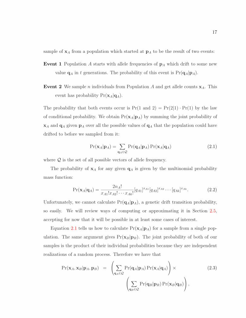
Figure 2.1: Diagmrammatic sketch of the scenario giving rise to the likelihood model.

pA1, . . . , pAk and pB1, . . . , pBk are the allele frequencies in the ancestral populations.

In t generations they drift to qA1, . . . , qAk and qB1, . . . , qBk, respectively. xA1, . . . , xAk

are the counts of alleles of di!erent kinds from a sample taken from Population A.

xA1, . . . , xAk are the same from Population B. NA and NB are the e!ective sizes of

the populations which we must assume to be known from historical population size

data. nA and nB are the respective number of individuals in each sample. The central

question in this study is represented by the large question mark—we do not know if

Populations A and B were one in the same t generations ago, or not.

17

sample of xA from a population which started at pA to be the result of two events:

Event 1 Population A starts with allele frequencies of pA which drift to some new

value qA in t generations. The probability of this event is Pr(qA|pA).

Event 2 We sample n individuals from Population A and get allele counts xA. This

event has probability Pr(xA|qA).

The probability that both events occur is Pr(1 and 2) = Pr(2|1) · Pr(1) by the law

of conditional probability. We obtain Pr(xA|pA) by summing the joint probability of

xA and qA given pA over all the possible values of qA that the population could have

drifted to before we sampled from it:

Pr(xA|pA) ="

qA!QPr(qA|pA) Pr(xA|qA) (2.1)

where Q is the set of all possible vectors of allele frequency.

The probability of xA for any given qA is given by the multinomial probability

mass function:

Pr(xA|qA) =2nA!

xA1!xA2! · · ·xAk![qA1]

xA1 [qA2]xA2 · · · [qAk]

xAk . (2.2)

Unfortunately, we cannot calculate Pr(qA|pA), a genetic drift transition probability,

so easily. We will review ways of computing or approximating it in Section 2.5,

accepting for now that it will be possible in at least some cases of interest.

Equation 2.1 tells us how to calculate Pr(xA|pA) for a sample from a single pop-

ulation. The same argument gives Pr(xB|pB). The joint probability of both of our

samples is the product of their individual probabilities because they are independent

realizations of a random process. Therefore we have that

Pr(xA,xB|pA,pB) =

#

$"

qA!QPr(qA|pA) Pr(xA|qA)

%

&" (2.3)

#

$"

qB!QPr(qB|pB) Pr(xB|qB)

%

& ,

18

giving us our full probability equation. Of course, we don’t know what pA and pB are,

though we do know xA and xB. So we consider our probability function as a function

of the parameters with the data treated as fixed, and this gives us the likelihood of

pA and pB given xA and xB (Edwards 1992).

2.3 The Likelihood-Ratio Test

With the likelihood L(pA,pB|xA,xB) = Pr(xA,xB|pA,pB) we can use an asymptotic

likelihood-ratio test for HA (the hypothesis that Population B descended exclusively

from fish planted from Population A) against the general alternative, HG, that some

proportion of the ancestry of B must not be from A. The likelihood ratio test statistic

is2:

" = 2 log

#

'$sup

pA,pB!PG

L(pA,pB|xA,xB)

suppA,pB!PA

L(pA,pB|xA,xB)

%

(& (2.4)

where PG is the set of values pA and pB may take under the general alternative

hypothesis HG, and PA is the set of values that pA and pB are constrained to under

the more restrictive null hypothesis HA. Under the general alternative hypothesis

pA and pB may take whatever values they want to so long as they still represent

frequencies of alleles (i.e., their components are between 0 and 1 and sum to 1).

Under the null hypothesis, however, both Population A and Population B originated

from the same population at time " = 0 and so pA and pB must be the same under

HA (i.e., PA = {pA,pB : pA = pB}).

Since PA is a subset of PG, the numerator in Equation 2.4 will never exceed the

denominator, and hence " will always be greater than or equal to zero. In fact,

when xA = xB, " will be zero. However, " increases as xA and xB become more

di!erent and we will reject HA when " is su#ciently large3. Theory on the asymptotic

2 For those unfamiliar with it “suppA,pB!PG” essentially means “the maximum over values of pA

and pB in the set PG”3 It may be helpful to note that this test statistic is a sort of fancily-dressed G-statistic (Sokal

19

distribution of log-likelihood ratios tells us how large " should be for us to reject HA

with a Type I error level of # (Kendall and Stuart 1979). If the null hypothesis

is true (pA = pB) and if the sizes of Population A and Population B, and the sizes,

nA and nB, of our samples increase toward infinity, the random variable " converges

in distribution to a chi-square random variable with $ degrees of freedom, %2! , where

$ is the di!erence in the number of free parameters under HG and HA. For a locus

with k alleles, there are 2(k#1) free parameters under HG, and k#1 free parameters

under HA, so in this case $ = k # 1.

In Lake Washington, of course, neither the sockeye populations nor our samples are

infinite. However, for reasonably large population and sample sizes a %2! distribution

closely approximates the distribution of " when HA is true. (I investigate this through

computer simulation in Section 2.9.) Therefore, if HA is true the probability that we

observe a " greater than some value, say d is Pr(%2! > d). If that probability is small,

then either 1) HA is true and a very rare event (observing such a large test statistic)

occurred; or 2) HA is not true so " does not have a %2! distribution, and our observed

test statistic is not so out of the ordinary. This, then, gives our test: reject HA if we

observe a " = d such that Pr(%2! > d) $ #.

Extending the test to multiple, independently segregating loci is straightforward.

For L such loci, indexed by j, the test statistic TL is the sum of the test statistics for

each locus

TL =L"

j=1

"j. (2.5)

TL is also chi-square distributed, but with degrees of freedom equal to the sum of the

degrees of freedom for each "j.

* * * * *

I have, to this point, presented the statistical method in skeletal form. The logic

and Rohlf 1981; Zar 1984). In fact, if there were no drift term in the likelihood function, this

would boil down to the well-known G-test for multinomial proportions.

20

behind the test should be clear from the above discussion, even though it remains to

fill in some details regarding the computation or approximation of transition proba-

bilities, and routines for maximizing the likelihood function. In the next six sections

I address these details, starting with some background on genetic drift and e!ective

population number.

2.4 Genetic Drift and E!ective Population Number

In order to compute the transition probability Pr(qA|pA) we must adequately model

genetic drift, a random evolutionary force acting upon allele frequencies. Genetic

drift occurs in populations of finite size because, as a result of random chance, some

parents have more o!spring than others, thus increasing the frequency of their genes

in the following generation. Fisher (1930) and Wright (1931) first described ge-

netic drift mathematically, using an idealized model of a randomly-mating population

subsequently known as a “Wright-Fisher” model.

The Wright-Fisher model is a population of constant size and discrete generations

(all individuals reproduce at the same age and die after reproduction) with each

individual having an equal probability of mating with any other individual or itself.

This mating scheme can be visualized for a population of N diploid individuals as

follows: 1) individuals produce gametes according to their genotype (so, for example,

half the gametes of a heterozygous Aa individual would be a’s and the other half

A’s), 2) at the time of mating, each individual contributes an infinite but equal

number of gametes to a “gamete pool,” 3) an individual of the next generation is

“assembled” by combining two gametes chosen at random from the gamete pool; N

such individuals are assembled. Note that as this process continues over generations,

alleles may be lost from the population. For example, if in one generation only 3

individuals carry copies of the a allele and none of these three produce o!spring, the

frequency of a in the next generation will be zero and we say that the population

21

has become “fixed” for the alternate allele, A. After the a allele is lost, its frequency

remains at zero, until it is reintroduced to the population via migration or mutation,

two processes we disregard for now.

Such a random mating scheme lacks realism for some organisms, but its simplicity

allows a number of important results. In order to understand these, it is necessary to

think of allele frequencies in future generations as random variables, and perhaps the

easiest way to do this is to think not of the e!ect of drift in a single population, but

rather in an infinite number of initially identical “replicate” populations, any one of

which may be an observed or realized population. For the case of two alleles, say A

at frequency p0 and a at frequency 1# p0, we see that X1, the number of A alleles in

the next generation, is a binomially distributed random variable: X1 % Bin(2N, p0)

(i.e., many of the replicate populations will have 2Npo alleles in the next generation,

but the others will have more or fewer than that, following a binomial distribution).

It follows that the expectation of the frequency of A in our replicate populations after

one generation of random mating is E(X12N ) = p0 and the variance of the frequency of

A across the replicate populations after one generation is Var(X12N ) = p0(1"p0)

2N . After

t generations of drift in a Wright-Fisher population, the expectation and variance of

the allele frequency Xt2N are:

E( Xt2N ) = p0 (2.6)

Var( Xt2N ) = p0(1# p0)

)

1#*1# 1

2N

+t,

(2.7)

The expectation is always the initial value p0, but the variance increases with each

generation until, as t & ' it reaches its limiting value of p0(1 # p0). (This limit

corresponds to the time when each replicate population has become fixed for either

the A or the a allele.) Notice that each generation the variance increases by 1/2N

of the distance left to its limiting value. In other words, a gene in a Wright-Fisher

population has a characteristic rate by which the variance of its frequency (considered

as a random variable—as a realization of possible allele frequencies in an infinite

22

number of replicate populations) increases, and that rate depends on the size of the

population. This provides an important way to relate the behavior of the allele

frequencies in natural populations to those of the idealized Wright-Fisher model,

using the e!ective population size (also called the e!ective population number).

Consider any natural or ideal population that violates the Wright-Fisher model

(but still with no selection or mutation). It may have two sexes, fluctuating popula-

tion size, overlapping generations, etc. (Felsenstein 1995). Though it may be much

more di#cult to calculate, the variance of the frequency of a gene in these popula-

tions will change through time at some rate. The variance e!ective size, Ne, of this

population is the size of a Wright-Fisher population that would show the same in-

crease in variance of allele frequency in the same amount of time. Many authors have

derived expressions for variance e!ective numbers in populations departing from the

Wright-Fisher model. For example, Crow and Denniston (1988) present formulae

for populations with two sexes versus a single sex and self-fertilization permitted ver-

sus excluded. In general, the derivations for variance e!ective numbers in di!erent

types of populations are more di#cult than they are for the more familiar inbreeding

e!ective number which is the size of a Wright-Fisher population that would give the

same rate of increase of probability of identity-by-descent of two gene copies taken

at random from the population. In many circumstances the variance e!ective size

equals the inbreeding e!ective size of a population. However, sometimes the two dif-

fer. Hereafter, “e!ective size” will be taken to be the variance e!ective size, as this

is the quantity that is most intimately associated with t-step transition probabilities

in the Wright-Fisher model.

In dealing with natural populations, though one could draw from a great many

formulae to obtain the e!ective number for di!erent scenarios, in actual practice

it is very di#cult to account for all of the ways that a natural population departs

from a Wright-Fisher model. Accordingly, since the early 1970’s, researchers have

empirically estimated the variance e!ective size of natural populations. They do this

23

by drawing genetic samples from a population at successive time points and using

the information in those samples to estimate the increase in allele frequency variance

over time.4 This increase in variance, then, converts into an e!ective population

number. Krimbas and Tsakas (1971) first employed this method to estimate the

e!ective size of olive fruit fly populations. Several authors have suggested statistical

refinements for estimating Ne empirically (Pamilo and Varvio-Aho 1980; Nei and

Tajima 1981; Pollak 1983), and more recently Waples (1989) presented a general

method that reconciles some of the di!erences between earlier techniques. Jorde

and Ryman (1995) proposed a method specifically for populations with overlapping

generations. Salmon researchers commonly use the methods of Waples (1989) to

estimate the e!ective number of spawners in salmon populations. Later, I will discuss

how to combine empirical estimates of e!ective number of spawners over many years

to estimate Ne for the Bear Creek Problem (Section 3.2).

One of the great advantages of converting the actual size of a population to its

e!ective size is that almost all of the theory on the behavior of genes and allele

frequencies has been formulated in reference to the Wright-Fisher model. Using the

e!ective size allows one to access many useful results. For the present problem, using

the e!ective size will allow us to compute genetic drift transition probabilities using

formulae that have been developed for the Wright-Fisher model.

2.5 t-Step Transition Probabilities in the Wright-Fisher Model

Genetic drift may cause allele frequencies to change each generation. The probability

that an allele frequency takes a particular value in the next generation depends only

on the population’s size and on the allele frequency in the current generation. In other

words, given the current allele frequency, the frequency in the next generation does

4 Such a technique is called a temporal method. Another approach sometime used with salmon

populations is the disequilibrium method (Bartley et al. 1992).

24

not depend on the frequencies in any of the previous generations. This property makes

genetic drift in a Wright-Fisher model a Markov stochastic process. In particular it

is a discrete time (the generations are discrete), finite (there are a finite number of

values the allele frequency may take) Markov chain (see Karlin and Taylor 1975).

As such, one can compute t generation transition probabilities exactly, but, in some

cases this requires very many computations. Some authors have developed di!usion

approximations to the process which are, unfortunately, di#cult to use in their most

accurate forms. However, under restricted conditions, simpler approximations are

valid and useful for statistical inference. I treat each of these topics in the subsections

below, outlining a sort of transition probability “toolkit” to have at our disposal for

Chapter 3.

2.5.1 Drift as a Markov Process

Given a Wright-Fisher population with N diploid individuals and two alleles A and

a at a locus, there are 2N + 1 allele frequency states that the population may be in:

it may have no copies of the A allele, 1 copy, 2 copies, and so forth up to 2N copies.

Since the number of A alleles in the next generation is binomially distributed, the

probability that a population with i copies of the A allele in the current generation

has j copies in the next generation is

Pi,j =

-2N !

j!(2N # j)!

. *i

2N

+j *1# i

2N

+2N"j

. (2.8)

We can arrange these probabilities into a one-step transition probability matrix, P(1):

P(1) = ||Pi,j|| =

#

''''''''$

P0,0 P0,1 · · · P0,2N

P1,0 P1,1 · · · P1,2N

......

. . ....

P2N,0 P2N,1 · · · P2N,2N

%

((((((((&

. (2.9)

This matrix is essentially just a table where the entry in the ith row and the jth

column is the probability of drifting from i to j copies of the A gene in one generation.

25

However, with P(1) we can easily obtain P(t), the t-generation transition probability

matrix, as the matrix product of P(1) with itself t times:5

P(t) = P(1)P(1)P(1) · · ·P(1)/ 01 2

t times

. (2.10)

In fact, the matrix P(t) would give us the values we need for Pr(qA|pA) and Pr(qB|pB)

in Equation 2.3 so long as there were only two alleles at the locus in question in Pop-

ulations A and B. If Populations A and B were Wright-Fisher populations these

transition probabilities would be exact and would properly reflect the way that prob-

ability mass accumulates at the boundaries due to allele fixation in the populations.

Even if A and B are not Wright-Fisher populations (as salmon populations certainly

are not), using the e!ective size to determine the Pi,j and the number of rows and

columns in P(1) should yield a reasonably accurate P(t) by (2.10). For modestly-

sized Wright-Fisher populations (say N < 250) with only two alleles, multiplying

the matrices is manageable. However, with more alleles the number of computations

required becomes prohibitively large.

If there are more than two alleles at a locus (i.e., if the vectors pA and pB

have three or more components), drift in a Wright-Fisher population is still a Markov

process but the number of states (combinations of allele frequencies) increases rapidly.

As before, computing the one-step transtition probability is easy; it is a multinomial

probability. Thus if there are k alleles A1, A2, . . . , Ak, and in the current generation

there are b1 alleles of type A1, b2 of type A2 and so forth, then the probability that

there are c1 type A1 alleles, c2 type A2 alleles and so forth in the next generation is:

Pr(c1, . . . , ck|b1, . . . , bk) =2N !

c1!c2! · · · ck!

-b1

2N

.c1 -b2

2N

.c2

· · ·-

bk

2N

.ck

. (2.11)

5 The reader may recognize that this says that p(t), a row vector of transition probabilities, may

be obtained by p(t) = p(0)P(t) (where p(0) is the vector of the starting state) and hence may

wonder why one doesn’t just find all the eigenvalues and left eigenvectors of P and compute p(t)

by such a spectral resolution approach. Unfortunately no one has discovered expressions for all

but two of the left eigenvectors of P (Felsenstein 1995).

26

Table 2.1: Number of allele frequency states for a diploid population of size N individ-

uals with 3,4,5, or 6 alleles. The number of states was obtained by direct evaluation

of the sum in (2.12) via a short, recursive, computer program.

k, the number of alleles

N 3 4 5 6

25 1,326 23,426 316,251 3,478,761

75 11,476 585,276 22,533,126 698,526,906

150 45,451 4,590,551 348,881,876 21,281,794,436

These one-step transition probabilities may also be arranged into a matrix, but there

are very many states to consider. For example, with three alleles and 2N = 200 a

population may have no A1 alleles, no A2 alleles, and 200 A2 alleles—a state that

can be denoted (0,0,200). Of course it could also be in state (1,2,197) or (1,3,196) or

(24,26,150). In fact there are 20,301 possible states, which is the number of ordered

triplets of whole numbers whose sum is 200. In general, for a population of N diploid

individuals and k alleles the number of states equals the number of ordered k-tuples

whose sum is 2N . This is the number of terms in the multinomial expansion of

(a1 + a2 + · · · + ak)2N and can be found as the sum:

2N"

i1=0

#

$2N"i1"

i2=0

#

$2N"i1"i2"

i3=0

· · ·2N"""

ik!1=0

1

%

&

%

& , (2.12)

where & = i1 + i2 + · · ·+ ik"2. I have computed the number of states for several values

of k and N (Table 2.1). Even for modest values of k and N the size of the matrix is

too large to realistically compute the t-step transition probability matrix by Equa-

tion 2.10. For example, with N = 75 and k = 4, just the memory required to store

all the entries in P(1) as 32-bit floating points would require over 1,370 gigabytes of

computer memory. There is little hope of obtaining the exact transition probabilities

from (2.10) for all but the smallest cases; instead we must use approximations.

27

2.5.2 Di!usion Approximations to Genetic Drift

Kimura (1955a, 1955b, 1956) derived approximations to genetic drift transition prob-

abilities by considering the allele frequencies as continuous random variables rather

than as discrete ones existing only in multiples of 1/2N . Other authors have re-

fined these approximations (Littler and Fackerell 1975; Griffiths 1979), but

their results are di#cult to implement. I have encountered no cases of statistical

inference using the complete density expressions from the above papers. However,

Cavalli-Sforza and Edwards (1967) noted from Kimura (1955a) that to a first

approximation, the transition probability density for multiple alleles is multinomial

in shape. This led to a useful approximation for drift in a multiallelic locus of allele

frequencies under stereographic projection.

2.5.3 Brownian Motion and Stereographic Projection

Edwards (1971) showed that drift can be approximated by Brownian motion in a

curved space which may be projected into a Euclidean space, giving very nice prop-

erties. This approach forms the basis of the well known Cavalli-Sforza and Edwards

“Arc” genetic distance, and allowed Thompson (1973) to compute likelihoods in-

volving drift transition probabilities.

The essence of this approximation lies in recognizing the geometrical interpre-

tation of the arc-sine square-root transformation on multinomial proportions, and

using the geometry to find a projection of the transformed allele frequencies into

a Euclidean space where multinomially distributed random variables are “uncorre-

lated.” It is impossible to visualize the geometric interpretation for the case of more

than three alleles, because it involves more than three dimensions. Nonetheless the

main points of the result can be visualized and drawn for two or three alleles as done

below. Here, I sketch some of the reasoning behind this remarkable result which was

proved by Thompson (1972).

28

Normal approximation and angular transformation. Start with a single locus

having k alleles in the frequencies p = (p1, . . . , pk). The numbers of each type of

allele (c1, . . . , ck), after one generation are multinomially distributed. For reasonably

large N and small t, however, Edwards (1971) and Cavalli-Sforza and Edwards

(1967) quoting a result in Kimura (1955a) indicate that after t generations the

allele frequencies (i.e., the ci/2N , which we will denote qi) are still approximately

multinomially distributed, but with variance after t generations given by Var(qi) !

(1# e"t/2N)pi(1# pi). The first order Taylor approximation of e"t/2N is 1# t/2N , so

to further approximation,

Var(qi) !tpi(1# pi)

2N=

pi(1# pi)

2N/t. (2.13)

Notice that this is exactly the variance of a proportion arising from 2N/t multinomial

trials6 with cell probabilities (p1, . . . , pk). Thus, the qi are approximately distributed

as the random variable X2N/t where X % Multinomial(2N/t,p).

By the Central Limit Theorem the allele frequencies after t generations converge

in distribution as 2N/t & ' to a multivariate normal random variable in k # 1

dimensions:

32N/t

*(q1, . . . , qk"1)# (p1, . . . , pk"1)

+D#& MVN(0,V) (2.14)

where 0 is the zero vector (0, . . . , 0) and V is the variance-covariance matrix having

diagonal elements Vii = pi(1 # pi) and o!-diagonal elements Vij = #pipj for i (= j.

And so, (q1, . . . , qk"1) is approximately multivariate normal:

(q1, . . . , qk"1) % MVN*(p1, . . . , pk"1),

t

2NV

+. (2.15)

We now have a normal approximation to the joint distribution of the qi, but the

variance of each qi is a function of its mean [by the pi(1 # pi) term in the Vii.] So,

6 We assume here that 2N/t is an integer—an innocuous assumption as we will soon be taking the

limit as 2N/t&' and losing the discrete character of the multinomial distribution altogether.

29

apply the angular transformation, obtaining the new random variables 'i = sin"1)qi

for i = 1, . . . , k# 1. Under this transformation, our vector of initial allele frequencies

(p1, . . . , pk"1) becomes " = ((1, . . . , (k"1) where (i = sin"1)pi, and by the Delta-

method we obtain:

('1, . . . , 'k"1) % MVN(",V#) (2.16)

with the elements of V# given by the standard formulas:

V #ii = ()'i/)qi)

2 t

2NVii =

*1

2)

pi)

1# pi

+2-

tpi(1# pi)

2N

.

= t/8N (2.17)

V #ij = Cov('i, 'j) =

)'i

)qi

)'j

)qjVij = # t

8Ntan 'i tan 'j, for i (= j (2.18)

Notice that the variances of the 'i are the same no matter “where they start from”

(i.e., they are not functions of the initial allele frequencies, "), and the correlation

between 'i and 'j is # tan 'i tan 'j.

The geometric interpretation of these 'i is important. Consider first the case of k =

2 alleles so that the subscripts may be dropped and we have q % N(p, tp(1# p)/2N)

which implies ' % N((, t/8N). We may represent these quantities on the portion of

the unit circle in the first quadrant of the Cartesian plane. Starting from the origin,

if you go up the y-axis)

p units and then to the right)

1# p you hit the unit circle

at a point that is ( units of arc-length (radians) along the unit circle from the x-axis

(Figure 2.2). Likewise, the point on the unit circle corresponding to a height of)

q

is ' radians along the circle. The distance along the circle between these points (call

them P and Q) is the arc-length ' # (. Since ' is normally distributed around (,

the density function of ' depends on the square of the arc-length between P and Q.

That is:

f('; () = (2*t/8N)"1/2 exp

4#(' # ()2

2t/8N

5

. (2.19)

It follows that the log of the density function equals

log f('; () = #1

2log(*t/4N)# (' # ()2

t/4N, (2.20)

30

Figure 2.2: A section of the unit circle. The horizontal and vertical axes give the

square root of the frequencies of the two alleles at a diallelic locus, where p is the

initial frequency of one of the alleles which drifts to a frequency of q. ' and ( are

arc lengths along the perimeter of the unit circle. ( is the mean about which ' is

normally distributed with variance independent of '. The deviation due to drift is

the change in arc length, ' # (.

and so the di!erence in log-density at the mean (Point P ) and at any other point Q is

#('#()2/(t/4N). And it should also be apparent that the di!erence in log-likelihood

between the maximum likelihood (̂ and any other estimate of (, say (̃, is equal to

#((̂# (̃)2/(t/4N).

With k = 3 alleles, we can represent a population’s allele frequencies as points on

the surface of a unit sphere (Figure 2.3), and with k > 3 we can plot the allele fre-

quencies on the surface of a k-dimensional hypersphere. Edwards (1971, p. 875) uses

the fact that the correlation between any 'i and 'j is # tan 'i tan 'j to demonstrate

that the level-curves of log density around a mean point P are k # 1-dimensional

hyperspheres in the curved space centered on P . (The same is true for level curves of

log-likelihood around the point of maximum likelihood.) Thus, the log of the density

between any point Q on the surface of the hypersphere and the mean point P is a

31

function of the great-circle distance between Q and P . Finally, since the di!erence

in the log of the joint density of ('1, '2, . . . , 'k"1) between the point ((1, (2, . . . , (k"1)

and the point (l # (1, (2, . . . , (k"1), which is l radians away, is easily seen to be

#l2/(t/4N) it follows that the change in log-density from the mean P to any point

Q, is, in fact, proportional to the square of the great-circle distance from P to Q.

Stererographic projection. The above shows that a population’s initial allele fre-

quencies may be represented as a point on the surface of a hypersphere. Genetic

drift is then a force that makes the population jiggle away from those initial values.

Its jiggles are equally likely in any direction on the surface of the hypersphere, and

the distance that it travels from its starting point is normally distributed. This is

like the di!usion of very small particles outward from their source in a still medium;

hence the name “Brownian motion approximation.” However, the process takes place

in a curved space, and it is desirable to be able to represent the points P and Q

Figure 2.3: Geometric interpretation of the angular transformation for three alleles.

The axes give the square roots of the allele frequencies for each of the three alleles.

32

in a Euclidean space. The solution is the same that cartographers have used for

centuries—project the curved space into a “flat” one. Ideally one could find a pro-

jection such that shapes were preserved (orthomorphy) and the arc length from P

to Q in the curved space was the same as the distance between the corresponding

points P $ and Q$ in the projected space. That is not possible, but the stereographic

projection is orthomorphic and lengths are only slightly distorted. Because of the

orthomorphy, things that are hyperspheres (i.e., the level curves of equal log-density

or log-likelihood) in the curved space will be hyperspheres in the new, Euclidean

space. And because the size of things is not too greatly distorted, the di!erence in

log-density (or likelihood) between P and Q in the curved space will be approximately

equal to the Euclidean distance between P $ and Q$, because

(great circle distance from P to Q)2

t/4N! (Euclidean distance from P $ to Q$)2

t/4N.

The plane of projection is a hyperplane of k # 1 dimensions which exists in k

dimensions (see Figure 2.4 for k = 2). Any point on the plane may thus be specified

by k Cartesian coordinates.7 The ith Cartesian coordinate of the point Q$ is given in

the appendix8 of Edwards (1971) as

q$i =2

6)qi +

31/k

7

1 +!k

1

3qi/k

# 1)k, (2.21)

and the ith Cartesian coordinate of the point P $ is

p$i =2

6)pi +

31/k

7

1 +!k

1

3pi/k

# 1)k. (2.22)

7 Thompson (1973) actually redefines a new set of k#1 axes that span the hyperplane of projection,

and defines the coordinates of the projected points on that set of axes. For our current purposes

the result is similar.8 The formula also appears on page 877 in the text of Edwards (1971) but contains a typographical

error.

33

Figure 2.4: Stereographic projection for a diallelic locus (an heuristic diagram, not

drawn to scale). The points P and Q are projected into P $ and Q$ on the “plane” of

projection (a line when k = 2) which is tangent to the circle at its intersection with

the line x1 = x2. The axes show the allele frequency coordinates, q$1, q$2, p

$1, p

$2, under

stereographic projection given by (2.21) and (2.22).

Finally since the Euclidean distance between P $ and Q$ is given by

6(q$1 # p$1)

2 + (q$2 # p$2)2 + · · · + (q$k # p$k)

27 1

2 ,

the log-density at Q, which is the log-density that a population starting with al-

lele frequencies p = (p1, . . . , qk) drifts to have allele frequencies q = (q1, . . . , qk) is

approximately

# k

2log(2*t/8N)#

!ki=1(q

$i # p$i)

2

t/4N, (2.23)

which is exactly the joint log-density we would expect to get for (q$i, . . . , q$k) if each

component q$i were independently a N(p$i, t/8N) random variable. So, to compute

a drift transition density for q starting from p, we need only transform (q1, . . . , qk)

to (q$1, . . . , q$k) and (p1, . . . , pk) to (p$1, . . . , p

$k) by Equations 2.21 and 2.22, and then

treat each q$i as if it were distributed normally with mean p$i and variance t/8N ,

independently of the other q$i. (Of course, the q$i are not independent; it is easy to

34

show that they must sum to)

k. However, in the present application, this does not

matter. We are just using the q$i to compute the log of the transition density from p

to q).

2.5.4 Other Approximations to Drift Probabilities

Thompson (1973) used the approximation just described to analytically obtain a

maximum likelihood solution to the proportion of Norse ancestry in the people of

Iceland. With the recent availability of computers, however, analytical solutions

are no longer so crucial. Numerical integration and maximization routines available

with many computer packages allow us to deal with such things as the covariance

between allele frequencies at a locus. Two such approaches that use computation

in place of analytical ingenuity are immediately apparent from the previous section.

The first method uses the normal approximation in Equation 2.15 to the density of

(q1, . . . , qk"1). This we will call the “Normal” method. The second method (call it

the “Angular” method) involves doing almost the same thing as the first, but uses

the angularly transformed variables (the 'i’s) and the relation in (2.16).

Another possibility for approximating likelihoods would be to use Monte Carlo

simulation (Diggle and Gratton 1984), and if one were to do this it would be

best to simulate collecting genetic samples [the Pr(xA|qA) term] in addition to the

genetic drift. This would involve simulating many replicates of genetic drift and

sample collection in two populations starting from allele frequencies pA and pB and

then using the proportion of outcomes with allele counts xA and xB to estimate the

likelihood L(pA,pA|xA,xB). But, since we ultimately shall wish to maximize this

likelihood over di!erent values of pA and pB, we would have to repeat the Monte

Carlo simulations starting from a number of di!erent pA’s and pB’s and compare the

Monte Carlo estimate of the likelihood from each of these separate simulations. Doing

so requires another Monte Carlo simulation for each di!erent set of starting allele

frequencies, and so would be called a “many samples” approach to maximizing the

35

likelihood (Geyer 1996). Such a technique would require a great deal of computation

for loci with many alleles because 1) there are so many possible final allele frequency

states (Table 2.1) that a good estimate of the probability would require very many

Monte Carlo replicates within any one sample, and 2) there are also very many initial

allele frequency states to consider maximizing the likelihood over, so one may have

to try many initial frequencies. It may be possible to make the second problem more

manageable by Markov Chain Monte Carlo. I do not pursue such an approach here.

2.6 Assessing the Approximations

In the last section we learned of four methods for computing transition probabilities

in a Wright-Fisher model—one exact method that is infeasible for complex cases,

and three related, approximate methods that rely on the asymptotic relationships

between transition probabilities, the multinomial distribution, and the normal distri-

bution. These approximations will be best for large population sizes and short time

spans (small t/2N), however we may want to apply these approximations to small

populations as well. This section explores how the approximations break down for

small populations. I compare the Normal and the Angular approximations9 to the

exact probabilities in small, computable cases (diallelic loci in small Wright-Fisher

populations). The results warn us of situations where the approximations are inap-

propriate.

Figure 2.5 shows the distributions of allele frequency for an allele starting at a

frequency of 0.5 and drifting for four and fourteen generations. (I have chosen four-

teen generations for these simulations because that is roughly the number of sockeye

salmon generations that passed between the introduction of Baker Lake sockeye to

Lake Washington and Hendry et al. (1996)’s genetic sampling.) These transition

9 I do not also compare the approximation from stereographic projection, because for a diallelic

locus it is quite close to the Angular method, di!ering only by the distortion due to the projection.

36

0 0.1 0.2 0.3 0.4 0.5 0.6 0.7 0.8 0.9 10

0.01

0.02

0.03

0.04

Prob

abilit

y

Ending Frequency

(a) 4 Generations

0 0.1 0.2 0.3 0.4 0.5 0.6 0.7 0.8 0.9 10

0.01

0.02

0.03

Prob

abilit

y

Ending Frequency

(b) 14 Generations

Figure 2.5: Probability distribution of allele frequency (initially 0.5) in a Wright-

Fisher population of size N = 50 after 4 and 14 generations, computed by Equa-

tion 2.10

probabilities look very much like binomial distributions with variance increasing over

time [just as Cavalli-Sforza and Edwards (1967) say they should for small t/2N ].

Accordingly, we expect that any of the approximations would work well here.

However, when we change the starting conditions we get a very di!erent result.

Figure 2.6 shows the distributions for another population of size N = 50 with a

starting allele frequency of 0.2. The distribution in Figure 2.6(b) no longer looks

37

0 0.1 0.2 0.3 0.4 0.5 0.6 0.7 0.8 0.9 10

0.01

0.02

0.03

0.04

0.05

0.06

Prob

abilit

y

Ending Frequency

Initial Frequency

(a) 4 Generations

0 0.1 0.2 0.3 0.4 0.5 0.6 0.7 0.8 0.9 10

0.01

0.02

0.03

0.04

0.05

0.06

Prob

abilit

y

Ending Frequency

Initial Frequency

(b) 14 Generations

Figure 2.6: Probability distribution of allele frequency in a Wright-Fisher population

of size N = 50 after 4 and 14 generations, having started from a frequency of 0.2. In

(b) note all the probability mass piled up at zero.

binomial. Most notably, after fourteen generations the probability that the frequency

is zero (i.e., that the allele has been lost from the population) is much higher than the

probability that only one copy of the allele remains, and the peak of the distribution

is not at the starting value of the allele frequency (it is shifted over by the length of

the dashed line). Both of these features present trouble for the approximations, as

we can see if we plot the approximations on the same axes as the exact probabilities

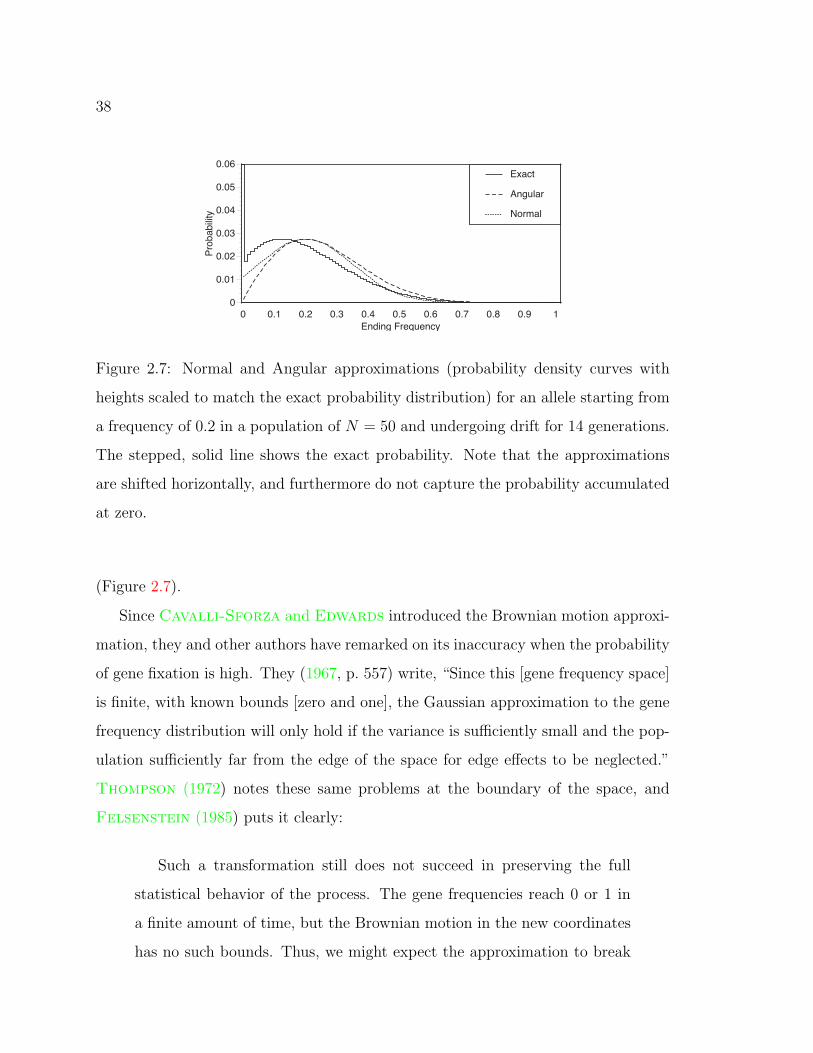
38

0 0.1 0.2 0.3 0.4 0.5 0.6 0.7 0.8 0.9 10

0.01

0.02

0.03

0.04

0.05

0.06

Prob

abilit

y

Ending Frequency

Exact

Angular

Normal

Figure 2.7: Normal and Angular approximations (probability density curves with

heights scaled to match the exact probability distribution) for an allele starting from

a frequency of 0.2 in a population of N = 50 and undergoing drift for 14 generations.

The stepped, solid line shows the exact probability. Note that the approximations

are shifted horizontally, and furthermore do not capture the probability accumulated

at zero.

(Figure 2.7).

Since Cavalli-Sforza and Edwards introduced the Brownian motion approxi-

mation, they and other authors have remarked on its inaccuracy when the probability

of gene fixation is high. They (1967, p. 557) write, “Since this [gene frequency space]

is finite, with known bounds [zero and one], the Gaussian approximation to the gene

frequency distribution will only hold if the variance is su#ciently small and the pop-

ulation su#ciently far from the edge of the space for edge e!ects to be neglected.”

Thompson (1972) notes these same problems at the boundary of the space, and

Felsenstein (1985) puts it clearly:

Such a transformation still does not succeed in preserving the full

statistical behavior of the process. The gene frequencies reach 0 or 1 in

a finite amount of time, but the Brownian motion in the new coordinates

has no such bounds. Thus, we might expect the approximation to break

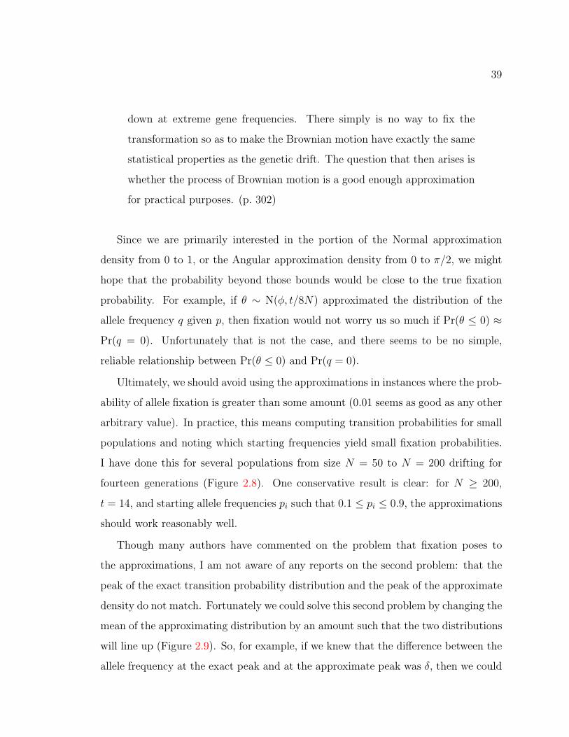
39

down at extreme gene frequencies. There simply is no way to fix the

transformation so as to make the Brownian motion have exactly the same

statistical properties as the genetic drift. The question that then arises is

whether the process of Brownian motion is a good enough approximation

for practical purposes. (p. 302)

Since we are primarily interested in the portion of the Normal approximation

density from 0 to 1, or the Angular approximation density from 0 to */2, we might

hope that the probability beyond those bounds would be close to the true fixation

probability. For example, if ' % N((, t/8N) approximated the distribution of the

allele frequency q given p, then fixation would not worry us so much if Pr(' $ 0) !

Pr(q = 0). Unfortunately that is not the case, and there seems to be no simple,

reliable relationship between Pr(' $ 0) and Pr(q = 0).

Ultimately, we should avoid using the approximations in instances where the prob-

ability of allele fixation is greater than some amount (0.01 seems as good as any other

arbitrary value). In practice, this means computing transition probabilities for small

populations and noting which starting frequencies yield small fixation probabilities.

I have done this for several populations from size N = 50 to N = 200 drifting for

fourteen generations (Figure 2.8). One conservative result is clear: for N * 200,

t = 14, and starting allele frequencies pi such that 0.1 $ pi $ 0.9, the approximations

should work reasonably well.

Though many authors have commented on the problem that fixation poses to

the approximations, I am not aware of any reports on the second problem: that the

peak of the exact transition probability distribution and the peak of the approximate

density do not match. Fortunately we could solve this second problem by changing the

mean of the approximating distribution by an amount such that the two distributions

will line up (Figure 2.9). So, for example, if we knew that the di!erence between the

allele frequency at the exact peak and at the approximate peak was !, then we could

40

00.1

0.20.3

0.40.5

0.60.7

0.80.9

1

0 0.05 0.1 0.15 0.2 0.25 0.3 0.35 0.4

Prob

abilit

y of

Fixa

tion

at Z

ero

Initial Gene Frequency

N = 50

N = 75

N = 100

N = 150

N = 200

Figure 2.8: Probability that allele frequency drifts to zero in 14 generations for five

di!erent population sizes and various initial frequencies.

0 0.1 0.2 0.3 0.4 0.5 0.6 0.7 0.8 0.9 10

0.01

0.02

0.03

0.04

0.05

0.06

Prob

abilit

y

Ending Frequency

Exact

Ang. Trans.

Normal

Figure 2.9: Normal and Angular approximations shifted so that the peaks match the

peak of exact probability for an allele starting from a frequency of 0.2 in a population

of N = 50 undergoing drift for 14 generations.

41

-0.1-0.08

-0.06-0.04

-0.020

0.020.04

0.060.08

0.1

0 0.1 0.2 0.3 0.4 0.5 0.6 0.7 0.8 0.9 1

Diffe

renc

e (d

elta

)

Initial Gene Frequency

10075 50

200150

Figure 2.10: Values of !, the horizontal distance between the peak of the exact tran-

sition probability distribution and peaks of the Angular and Normal approximation

densities for t = 14 generations. Numbers next to the lines indicate population sizes

N ; the x-axis is the starting allele frequency.

define ' % N(sin"1)p + !, t/8N) so that the peak was in the right place. Of course, to

do this we must know what ! is, and, currently, that means computing the transition

probabilities exactly and seeing how far the peak of the distribution is from its mean.

(By that time one may just wish to use those exact probabilities, for a diallelic locus,

at least.) I have calculated ! after fourteen generations for several population sizes,

up to N = 200, from all the possible starting allele frequencies (Figure 2.10). From

the graph it is apparent that ! may be quite large for small N , but for N * 200 with

a starting frequency between 0.1 and 0.9, ! will not be greater than about 0.02 in

magnitude. Furthermore we will see in Section 2.9 that the !-shift seems to have very

little e!ect on the value of the test statistic, ".

On a final note, Figure 2.9 shows that the Angular approximation is closer to

42

the exact probability than is the simple Normal approximation. This seems to be

the case for most starting frequencies between zero and one. (Though the Normal

approximation appears better for an initial allele frequency of 0.5, the di!erence is

not so great). I prefer the Angular approximation for this reason.

2.7 Adding the Sampling Step

The last two sections showed ways to compute t-generation transition probabilities.

We need those techniques to calculate the Pr(qA|pA) and Pr(qB|pB) terms in the joint

likelihood equation (2.3 on Page 17). But now, we must use those transition proba-

bilities (or the approximations) to obtain the probability of a sample of genes from

the population. There are two ways to go about this. The first follows Equation 2.1,

in spirit, and returns a discrete probability for the sample. I call this a sample mass

method. The second method returns a probability density for the sample. Such a

sample density method requires less computation, but may be inappropriate in some

circumstances.

2.7.1 Sample mass methods

With exact transition probabilities. It is not di#cult to add the sampling step to

transition probabilities computed exactly by Equation 2.10. Since it is only feasible

to use (2.10) for diallelic loci, we will only use this method to find Pr(x|p), where x,

the number of alleles of a particular type in a sample of n individuals, and p, the gene

frequency t generations ago, are scalars (not vectors as they are for multi-allelic loci).

Having computed P(t), our t-step transition probability matrix (see Section 2.5.1),

we can express the sum in (2.1) compactly in matrix notation. Define a 2N + 1-

dimensional column vector c(1) of binomial probabilities corresponding to Pr(x|q)

(remember, x is a known quantity, here) for di!erent values of q such that the ith

43

component of c(1) is Pr(x|q = i"12N ):

c(1) =*Pr(x| 0

2N ), Pr(x| 12N ), Pr(x| 2

2N ), . . . , Pr(x|2N2N )

+T

, (2.24)

where the superscript T means matrix or vector transpose. Then, compute

c(t) = P(t)c(1). (2.25)

The column vector c(t) then has 2N+1 components, and its ith component is Pr(x|p =

i"12N ). Hence the maximum likelihood is just the value of the largest component of c(t).

Given our two samples, A and B, we may find c(t)A and c(t)

B, having ith components

ctAi and ct

Bi respectively (the superscript t denotes “at time t”, not “to the tth power.”).

We can also define a joint likelihood column vector c(t)J with components ct

Ji = ctAic

tBi.

The likelihood ratio of (2.4) for a single locus is then

" = 2 log

#

$max

ictAi " max

ictBi

maxi

ctJi

%

& . (2.26)

When the sizes of Populations A and B are equal and small, this is a very fast

method once P(t) has been computed. When the populations are not of the same

size, however, some sort of interpolation of likelihoods becomes necessary and the

method loses much of its simplicity.

With the Normal approximation. Even if we use a continuous approximation

to the transition probability like our Normal approximation, we can still obtain a

discrete probability for our sample by integrating over the approximate density for

q. If we substitute the appropriate expressions into (2.1), drop the A subscripts (for

notational hygiene), and recognize that the discrete sum in (2.1) becomes an integral

over the continuous variable q, we get

Pr(x|p) =8 1

0· · ·

8 1

0f

*(q1, . . . , qk"1);p,

t

2NV

+· 2n!

x1! · · ·xk!

-k9

i=1

qxii

.

dq1 · · · dqk"1

(2.27)

44

where f is the joint density function for the multivariate normal distribution. The

second half of the integrand is the multinomial probability of the sample, and qk =

1#!k"11 qi. The above integral is analytically intractable, and with large k may be

di#cult to evaluate numerically.

With the Angular approximation. An expression similar to (2.27) may be derived

from the joint distribution of the 'i for the case of k alleles. For the special case of a

diallelic locus the sample mass approximation is

Pr(x|() =8 #/2

0f('; () · 2n!

x!(2n# x)!(sin2 ')x(cos2 ')2n"xd'. (2.28)

Here, ( = sin"1)p is our parameter, f is the univariate normal density of ' given

( and the second half of the integrand is a binomial probability (see that p = sin2 '

and 1# p = cos2 ').

Computing Pr(x|p) by a sample mass method with the approximation in the

stereographically projected space is di#cult and of limited utility, and we will not

consider it here.

2.7.2 Sample Density Methods

Rather than compute a discrete probability for our sample, we could compute a

density for it. This requires approximating the multinomial sampling of our genetic

samples with a normal distribution. In this way, drawing our samples is like one more

generation of drift. In other words, if x = (x1, . . . , xk) are the allele counts at a locus

in a sample of n diploid individuals from a population that had allele frequencies p

at some “starting” time in the past, then the sample allele frequency of each allele,

xi/2n, i = 1, . . . , k, has mean pi with an error due to drift and an error due to

sampling:

xi/2n = pi + +di + +si. (2.29)

Here, +d is the deviation due to genetic drift, and +s is the deviation due to sampling.

45

Such a scheme works well with the stereographically projected space (Thompson

1973). If instead of dealing directly with the xi/2n we use their coordinates in the

projected space [i.e., substitute xi/2n for qi in (2.21) to get (xi/2n)$ ], then the log-

density of these transformed sample allele frequencies is, analogously to (2.23),

# k

2log(2*(t/8N + 1/8n))#

!ki=1[(xi/2n)$ # p$i]

2

t/4N + 1/4n. (2.30)

This works because the angular transformation makes the variance of each (xi/2n)$

independent of its mean and the stereographic projection takes care of the correlations

between alleles.

We could also use the Normal approximation (2.15) and Angular approximation

(2.16) to yield a sample density method. However, doing so in the case of multiple

alleles is much clumsier than using the stereographically projected space, because

there are conditional variances to get straight with the Normal approximation (i.e.,

the variance added in the sampling step depends on how far the allele frequencies have

drifted from p) and covariances to worry about with the Angular approximation.10

Fortunately, for a diallelic locus, we may find the density for an angularly transformed

sample frequency, sin"13

x/2n; it is approximately N((, t/8N + 1/8n). This should

be slightly more accurate than using (2.30) as it does not include the distortion

of the stereographic projection. Such a sample density method using the Angular

10 Long (1991) uses an iteratively reweighted least squares method to estimate admixture propor-

tions in human populations. He considers the sample allele frequency to depend on a drift error

term and a sampling error term (i.e., xi/2n = pi + !di + !si), but he does not state exactly how

these errors are distributed. Given the close correspondence between iteratively reweighted least

squares and the EM algorithm with a normal model, Long seems to be implicitly adopting a

multivariate normal approximation to allele frequency drift. However, he assumes that the !d and

!s are independent. (In practice, so long as the sample size is large, this is a fair assumption. See

the footnote on Page 49.)

46

approximation gives the test statistic, after a good deal of simplification, of

" =

6sin"1

3xA/2nA # sin"1

3xB/2nB

72

,21 + ,2

2

(2.31)

where ,2i = t/8Ni + 1/8ni.

2.8 Sampling with Recessive or “Null” Alleles

Up to this point we have assumed that all alleles are codominant; that they are

detectable in both heterozygous or homozygous form. When this is the case, then a

sample of n diploid, Wright-Fisher individuals is equivalent to a sample of 2n gene

copies from a population. Sometimes, however, recessive alleles at a locus are not

observable in all phenotypes and we are forced to estimate the frequency of such an

allele by the proportion of certain classes of phenotypes that we can observe in the

sample. Such a situation occurs, for example, with the LDH–A1* locus in some Lake

Washington sockeye populations. At that locus, heterozygotes of the common (*100)

allele and the *500 allele [called *NULL in Hendry (1995)] are indistinguishable from

*100 homozygotes. Nonetheless *500 homozygotes are detectable and the sample

proportion of such homozygotes contains information about the frequency of the

allele in the population.

For loci with recessive alleles we must adjust the probability function for our

samples. In general, the recessive nature of an allele does not a!ect the rate at

which it drifts in a Wright-Fisher population. Therefore, only the sampling step is

a!ected by lack of codominance, and so we need only redefine the probability of our

samples given q, the present-day population allele frequency of the recessive allele.

The following treats only diallelic loci with one dominant and one recessive allele.

This treatment will su#ce for the data of Hendry et al. (1996).

First, rather than observing allele counts x, we now observe only the number y

of recessive homozygotes in our sample. Assuming Hardy-Weinberg equilibrium, the

47

probability of drawing a recessive homozygote is q2. Thus the probability of drawing

y such recessive homozygotes in our sample of n individuals is:

Pr(y|q) =n!

y!(n# y)!

6q2

7y 61# q2

7n"y. (2.32)

We can immediately use this in our sample mass methods. If using the exact transition

probabilities from (2.10) then we may compute the likelihood ratio exactly as in (2.26)

except that we must now define c(1) in (2.25) to be a 2N+1 dimensional column vector

with the ith component given by Pr(y|q)—a binomial probability from the distribution

Bin(n, ( i"12N )2).

Adjusting the sample mass method under the Angular or Normal approximations

is similar. All that changes is the term in the integrand corresponding to the sampling

step. The Angular approximation sample mass method gives:

Pr(y|() =8 #/2

0f('; () ·

-n!

y!(n# y)!

.

(sin4 ')y(1# sin4 ')n"yd'. (2.33)

(Compare to Equation 2.28 on Page 44.)

2.8.1 A Sample Density Method for Null Alleles

Thompson (1973) notes the problem that recessive alleles pose to the Brownian

motion approximation under stereographic projection. She writes,

In fact this [likelihood model] applies only in the case where there

are su#cient antisera for all genotypes to be identifiable and the sample

gene frequencies known, but it remains a good approximation in all cases

provided the gene frequencies used are the maximum likelihood estimates

from phenotype data. (p. 72)

Indeed, the approximation is quite good for those cases where the frequency of the

recessive allele is not very low. However, when the recesssive allele is at a low fre-

quency, the approximation deteriorates mildly. I derive a more accurate Normal

48

approximation to the sample density for a diallelic locus with one recessive allele, by

noting that the asymptotic distribution of the maximum likelihood estimator (mle),

q̂, of q given y recessive homozygotes gives the asymptotic distribution of the sample

statistic3

y/n given q. We then can argue that the marginal distribution of3

y/n

(i.e., its distribution given p) will be approximately normal with a variance that can

be computed from its conditional variance and its conditional expectation given q.

Suppose that q is the frequency of allele A in a population at time t, and let

each individual in our sample represent an independent random variable Wi, i =

1, . . . , n. W = 1 if the individual is a recessive homozygote, and W = 0 otherwise.

Assuming Hardy-Weinberg equilibrium, the probability of drawing a homozygous,

AA individual is q2. Hence the probability of W = (W1, . . . , Wn) given q is

fW(w; q) =6q2

7!Wi

61# q2

7n"!

Wi(2.34)

Writing!

Wi as y gives the log of the probability of the n-sample as

log fW(w; q) = 2y log q + (n# y) log(1# q2). (2.35)

It is clear that the maximum likelihood estimate :q2 = y/n. Hence, by the invariance

of maximum likelihood estimators to transformation, q̂ =3

:q2 =3

y/n, and asymp-

totically, q̂ will be normally distributed with mean q and variance 1/In(q) where In(q)

is the Fisher Information for q in an n-sample and may be obtained from

In(q) = #E

-)2

)q2log fW(w; q)

.

=4n

1# q2. (2.36)

Immediately we have that3

y/n is distributed N (q, (1# q2)/4n), asymptotically.11

And so, letting v =3

y/n for notational ease, E(v|q) = q and Var(v|q) = (1#q2)/4n.

11 In fact, I realize now that this is more easily derived by the Delta-method: y/nD#& N(q2, q2(1#

q2)/n) implies by the Delta-method that;

y/nD#& N(q, (q2(1#q2)/n)"(1/4q2)) giving

;y/n

D#&

N(q, (1# q2)/4n).

49

That gives us v|q but we’d like the marginal distribution of v which we can write

“v|p” to emphasize that this is the distribution of v given p. We have already seen that

given p, q % N(p, tp(1 # p)/2N), approximately. So, as before, if we let +d = q # p

and +s = (v|q) # q, then both +s and +d are normally distributed. It follows that

v = p + +d + +s, being the sum of normals, is also normally distributed. We can

find the variance of v from the conditional variance, Var(v|q), and the conditional

expectation, E(v|q). By the customary relation,

Var(v|p) = E*Var(v|q)

++ Var

*E(v|q)

+, (2.37)

we find that,

Var(v|p) =*1# 1

4n

+tp(1# p)

2N+

1# p2

4n. (2.38)

And if our sample size is large,12 then 1# 1/4n ! 1 and we have that

v =3

y/n % N

-

p,tp(1# p)

2N+

1# p2

4n

.

, (2.39)

which gives us our sample density for a diallelic locus with one recessive allele. Note

that there are no transformations that do not involve N and n which will stabilize

the variance in this distribution. Therefore it is not possible to continue from here to

the angular transformation and stereographic projection. However, with computers

and numerical maximization routines this is a manageable approximation for testing

HA and HC .

2.9 The Distribution of the Test Statistic

As noted much earlier in this chapter (Page 18), the distribution of the test statistic

" is asymptotically that of a chi-square random variable. Of course, our populations

and samples are not infinite, so I have performed a series of simulations to determine

12 This is essentially the argument that validates the assumption by Long (1991) that !d and !s

are independent (see my footnote on Page 45).

50

how well the chi-square distribution fits the empirical distribution of ". I simulated

drift in two Wright-Fisher populations, A and B, each of size NA = NB = 100, and

each starting with the same allele frequency in a diallelic locus (.40, .25, .10, or .05,

depending on the simulation). After simulating drift in each population for fourteen

generations, I drew samples of size nA = nB = 50 from each population and then com-

puted the test-statistic " by both Equation 2.26 (Figure 2.11) and by Equation 2.31

(Figure 2.12). An e!ective size of 100 is relatively small as are samples of size 50.

I chose these values to explore scenarios in which the asymptotic distribution of the

test statistic might not be a good approximation. The approximation will improve

if N and n are larger. I performed 50,000 replicates for each of the four starting

frequencies.

Under this simulation scheme, both populations start with the same allele fre-

quency, and so the null hypothesis for our test statistic (pA = pB) holds. Thus the

distribution over the 50,000 replicates of the observed "’s should be approximately

chi-square with one degree of freedom. Since the asymptotic distribution of likeli-

hood ratios is closely related to the asymptotic distribution of maximum likelihood

estimates (Kendall and Stuart 1979, p. 247), we expect that the chi-square ap-

proximation will fail in those same instances where the Normal Approximation to

transition probabilities fails. In fact, this is what we observe. At low starting fre-

quencies, (.05 and .10) where we expect the probability of allele fixation to be high

and the distribution of allele frequencies after genetic drift to be non-normal, the

empirical distribution of " strays considerably from that of a %21 random variable.

However, for starting frequencies of .25 and .40 (from which the probability of allele

fixation in 14 generations for a population of N = 100 is negligible—see Figure 2.8)

the observed distribution of " computed both by the exact method and by the Angu-

lar approximation sample density method is extremely close to that of a %21 random

variable (Figures 2.11 and 2.12).

And, in fact, Figures 2.11(d) and 2.12(d) are somewhat unfair to our test statistic.

51

0 1 2 3 4 5 60

0.05

0.1

0.25

Prop

ortio

n / P

roba

bility

Test Statistic / Chi-square Value

SimulationChi-square

(a) Starting Frequency .40

0 1 2 3 4 5 60

0.05

0.1

0.25

Prop

ortio

n / P

roba

bility

Test Statistic / Chi-square Value

SimulationChi-square

(b) Starting Frequency .25

0 1 2 3 4 5 60

0.05

0.1

0.25

0.3

Prop

ortio

n / P

roba

bility

Test Statistic / Chi-square Value

SimulationChi-square

(c) Starting Frequency .10

0 1 2 3 4 5 60

0.05

0.1

0.250.3

Prop

ortio

n / P

roba

bility

Test Statistic / Chi-square Value

SimulationChi-square

(d) Starting Frequency .05

Figure 2.11: Simulated test statistic (") values compared to the chi-square distri-

bution with one degree of freedom. " was computed by the exact method (2.26).

Columns are a histogram of simulated "’s over 50,000 replicates. Figures a–d are re-

sults for di!erent starting frequencies. (See text for further explanation of simulation

methods.) Note that the test statistic is very closely chi-square distributed except

when the starting frequency is such that the probability of allele fixation is high (see

Figure 2.8).

52

0 1 2 3 4 5 60

0.05

0.1

0.25

Prop

ortio

n / P

roba

bility

Test Statistic / Chi-square Value

SimulationChi-square

(a) Starting Frequency .40

0 1 2 3 4 5 60

0.05

0.1

0.25

Prop

ortio

n / P

roba

bility

Test Statistic / Chi-square Value

SimulationChi-square

(b) Starting Frequency .25

0 1 2 3 4 5 60

0.05

0.1

0.25

Prop

ortio

n / P

roba

bility

Test Statistic / Chi-square Value

SimulationChi-square

(c) Starting Frequency .10

0 1 2 3 4 5 60

0.05

0.1

0.250.3

Prop

ortio

n / P

roba

bility

Test Statistic / Chi-square Value

SimulationChi-square

(d) Starting Frequency .05

Figure 2.12: Simulated test statistic (") values compared to the chi-square distribu-

tion with one degree of freedom. " was computed by the sample density method of

(2.31). Columns are a histogram of simulated "’s over 50,000 replicates. Figures a–d

are results for di!erent starting frequencies. (See text for further explanation of sim-

ulation methods.) Note that even with the sample density method the test statistic

is very closely chi-square distributed except when the starting frequency is such that

the probability of allele fixation is high (see Figure 2.8).

53

0

0.2

0.4

0.6

0.8

1

0 1 2 3 4 5 6

Cum

ulat

ive P

ropo

rtion

Test Statistic / Chi-square Value

Chi-squarecdfExactMethodDensityMethod

Figure 2.13: Cumulative proportion of test statistics (computed either by the exact

method of Equation 2.26 or by the Angular approximation sample density method of

Equation 2.31) versus the cumulative distribution function for a %21 random variable.

50,000 replicates with a starting frequency of .05.

Due to the discrete nature of the drift process, there are only certain values that

the test statistic may take. Accordingly there are big spikes and empty columns in

the graph. Comparing the observed cumulative proportion of " to the cumulative

distribution function of a %21 gives a better sense of the how well the approximation fits

(Figure 2.13). This clearly shows that the distribution of the test statistic is skewed

toward larger values (to the right) relative to the chi-square distribution. Perhaps

even more remarkable, though, is the fact that the distribution of " computed by

the sample density method using the Angular transformation, is much closer to the

chi-square distribution than the distribution of " computed exactly. This certainly

argues for the routine use of the sample density method and Angular or stereographic

projection approximation for loci with codominant alleles.

A final observation is that the horizontal distance (!—see Page 39) between the

peak of the Angular and Normal approximations and the peak of the exact transition

probability does not seem to a!ect the distribution of " when the starting frequency

54

is either .4 or .25, even though for N = 100, t = 14 and a starting frequency of .25, !

is as large as .03 (see Figure 2.10). Thus it appears that we need worry little about

! in most cases; so long as the probability of allele fixation is not high, it seems to

have little e!ect on the distribution of ".

2.10 Review of Assumptions

The proposed statistical technique makes a number of assumptions. It is important

to clarify these assumptions in the context of the biology of the situation and to

address how robust the method is to violations of them.

To start with, we have made the “standard” genetics assumptions: the markers we

use 1) are not subject to mutation, 2) are not subject to selective pressure, and 3) are

independently segregating. The first is a reasonable assumption for allozyme markers

on the time scales we are interested in, as the mutation rate of allozyme markers is

low (Nei 1987). The second assumption is also reasonable; the allozyme loci typically

used in salmon population genetic studies appear to be selectively neutral (Utter

et al. 1987). Finally, since sockeye salmon possess a large number (56 to 58) of

chromosomes (Allendorf and Thorgaard 1984) we are unlikely to violate the

assumption of independent segregation between loci.

Next, we have made several assumptions regarding the populations involved.

First, each of Populations A and B is assumed to be panmictic (well-mixed dur-

ing reproduction) among their NA and NB members (i.e., there is not population

subdivision). In practice this assumption is closely linked to how one converts his-

torical spawner counts into an e!ective population size. We also assume that A and

B are reproductively isolated from one another. That is, since the time of possible

introduction of individuals of A into the locale of Population B, there has been no

migration between the two populations (or other populations). In the case of Bear

Creek, it is unlikely that fish from either Baker Lake or Cultus Lake have strayed

55

to the Bear Creek system in recent years because sockeye home to their natal lake

system with great fidelity (Wood et al. 1994). It may not be so unlikely that descen-

dants of Baker Lake fish in the Cedar River or Issaquah Creek have strayed into Bear

Creek, as straying between tributaries within natal lake systems seems to occur at a

higher rate than straying between lake systems (McCart 1970; Wood et al. 1994).

However, any such straying, if it resulted in successful gene flow, would only make the

hypothesis test more conservative; migration would only reduce the allele frequency

di!erences between populations, thus decreasing the test statistic and reducing the

probability of rejecting the null hypothesis.

We also assume that our samples are representative of the population. This as-

sumption is related to the panmixia assumption above.

Finally, the heaviest assumptions that we require are those regarding the e!ective

sizes of Populations A and B as inputs to the likelihood model. We assume that

historical population size data are available and that such data may be reliably con-

verted into e!ective sizes. Furthermore, once in the model, we treat those e!ective

sizes as known without error, when, in fact, they are estimates themselves which

carry some uncertainty. In practice, one would hope to be able to use a reliable lower

bound on N in the model (since the test is more conservative for smaller N). For

Baker and Cultus Lakes, where comprehensive population data are available, this

is possible. Unfortunately, for the possibly introduced population (B in the model;

Bear Creek in the particular example) the very nature of the problem is such that

it is unlikely that there will be good population size data for the period soon after

introduction of individuals from A. This is certainly the case for Bear Creek, where

reliable population estimates exist only after 1981. Nonetheless it is possible to make

reasonable guesses at the historical e!ective size in Bear Creek given some scenarios

of its population history. I discuss this in the next chapter.

Chapter 3

THE STATISTICAL METHOD IN PRACTICE

The previous chapter described several ways to compute the likelihood ratio statis-

tic for the hypotheses that the sockeye in Bear Creek descended exclusively from fish

planted from Baker Lake (HA), or exclusively from Cultus Lake (HC). In this chap-

ter, we test HA and HC using the previously-collected data of Hendry et al. (1996).

The first section introduces the genetic data and tells how we combine them into a

form that we can readily use. Next we must use computer simulations to determine

the historical e!ective size of the salmon populations in Baker Lake, Cultus Lake, and

Bear Creek from records of spawner return number. Finally we conduct the tests,

and discuss the results.

3.1 Data for Baker and Cultus Lakes and Bear Creek

In 1992 and 1993, Andrew Hendry collected tissues from anadromous sockeye in seven

populations and performed gel electrophoresis on those samples. His data, at the four

loci which contained an alternate allele at a sample frequency q * .05 in at least one

of the populations, for Bear and Cottage creeks and Baker and Cultus lakes appear in

Table 3.1. The sample frequencies for all four loci in the populations sampled did not

di!er significantly between the two years (Hendry 1995, p. 26). So, for the present

analyses, we will consider the two samples from two years to be one large sample from

a single year as shown in the “pooled data” of Table 3.1. I have also pooled the data

from Bear and Cottage creeks together, treating the fish that spawn in those creeks

as part of a single, panmictic “Bear Creek System” population. This is reasonable

57

Table 3.1: Sample allele frequencies from Hendry et al. (1996) at four loci in Baker

and Cultus Lakes, and Bear and Cottage Creeks. n is the sample size in number of

diploid individuals for each locus. The frequency of the alternate (*100) allele at each

locus is not listed, but is 1 minus the sum of the frequencies of the other alleles at

the locus. POOLED DATA are the allele frequency estimates after pooling the data

between years and combining Bear and Cottage Creeks into a single “Bear Creek

System” population. COUNT DATA are the actual counts, x, of codominant alleles

out of 2n gene copies, or the counts, y, of recessive homozygote phenotypes out of n

individuals in the pooled samples.

ALAT* PGM–1* PGM–2* LDH–A1*

Popln. Year n *91 *95 n *NULL n *136 n *500

Baker 1992 40 0.563 0.075 39 0.320 56 0.170 56 0.000

1993 43 0.512 0.047 40 0.387 64 0.117 64 0.000

Cultus 1992 40 0.050 0.000 40 0.962 40 0.175 64 0.000

Bear 1992 40 0.225 0.150 40 0.671 63 0.127 40 0.224

1993 43 0.279 0.163 40 0.592 52 0.154 12 0.408

Cottage 1992 40 0.375 0.113 40 0.632 52 0.144 40 0.158

1993 40 0.213 0.088 40 0.689 40 0.138 38 0.281

+ POOLED DATA +

Baker 92,93 83 0.537 0.060 79 0.356 120 0.142 120 0.000

Cultus 1992 40 0.050 0.000 40 0.962 40 0.175 64 0.000

Bear-Cot 92,93 163 0.273 0.129 160 0.647 207 0.140 130 0.248

+ COUNT DATA +

Popln. Year 2n *91 *95 n *NULL 2n *136 n *500

Baker 92,93 166 88 10 79 20 240 34 120 0

Cultus 1992 80 4 0 40 37 80 14 64 0

Bear-Cot 92,93 326 89 42 160 67 414 58 130 8

58

as Bear and Cottage creeks are adjacent tributaries, and the gene frequencies in the

two populations are not significantly di!erent.

Underlying the sample estimates of allele frequency are the counts, x, of codomi-

nant alleles for PGM–2* and ALAT* or counts y of recessive homozygotes for the loci

with recessive alleles (PGM–1* and LDH–A1*). These counts appear in the table as

well.

3.2 Determining E!ective Sizes of the Populations

We defined the statistical method of Chapter 2 in reference to a Wright-Fisher pop-

ulation of size N . To apply the method to a real population we must determine

its variance e!ective size, Ne, from historical census data, and use that in place of

N in all the equations. Sockeye salmon populations depart from the Wright-Fisher

model at two di!erent levels. At the first level are those di!erences that occur in

a single year of reproduction: salmon on spawning grounds are not random-mating,

random-surviving individuals. For example, larger females generally produce more

eggs, and, presumably, then produce more o!spring (Burgner 1991). Additionally,

some pairs of parents will have more o!spring than others which return to reproduce

in future years, due to factors other than random chance (Waples 1990). Conse-

quently the e!ective number of spawners, Ns, in a particular year is less than the

number of individuals Ni counted on the spawning grounds. Researchers using the

temporal method and the disequilibrium method estimate that Ns is between 0.2Ni

and 0.7Ni for six chinook salmon, O. tshawytschwa, populations in the Snake River

basin (Waples et al. 1993). The lower end of those estimates (i.e., Ns/Ni ! 0.2 to

0.33) are probably more reliable (Robin Waples, National Marine Fisheries Service,

Northwest Fisheries Science Center, pers. comm.). Equivalent numbers for sockeye

salmon are, not available, but we assume that they are close to those for chinook.

At the second level of departure from the Wright-Fisher model, sockeye salmon

59

populations have overlapping year classes, so that the fish on the spawning grounds

in any one year represent only a part of the whole population, and the run sizes di!er

each year (Figure 3.1). There is currently no analytical framework to find the variance

e!ective size of a population with both fluctuating year-class size and overlapping year

classes or generations (Joe Felsenstein, University of Washington, Department of

Genetics, pers. comm.). However, given data on salmon run-sizes and age composition

of a salmon population over some time period, one can simulate the process of drift,

estimate the increase in allele frequency variance from the results and use that to

estimate the e!ective size of the population. Such simulations are similar to those in

Waples (1990) except that the present ones incorporate fluctuating population size.

Given the situation in Figure 3.1, it would be easy to simulate the progression of

the population through time, if at every year along the way we knew how many of

the spawners were three, four, or five years old. Though such information is seldom

available, we can usually make an educated guess about the proportion of individuals

in each year class that will reproduce at age three, four, or five. These proportions

are the quantities #3, #4, and #5 in Figure 3.1. The #’s and several assumptions

Figure 3.1: A population with overlapping year classes and fluctuating population

size. At time t there are Nt e!ective spawners made up of $5 individuals from time

t#5, $4 from t#4, and $3 from t#3. The o!spring of the spawners at time t mature

at three di!erent ages; a proportion #3 mature at three years, #4 at four years, and

#5 at five.

60

about survival rates of fish from di!erent year classes allow some simulation results.

3.2.1 Baker Lake Simulations

For Baker Lake, I have performed simulations based on a survival scheme in which,

if there are Nt e!ective spawners at year t, then $i, the number of e!ective spawners

that were born i years before, is given by Nt$iNt!i

!̄ where $̄ =!5

i=3 #iNt"i. This

is equivalent to assuming that each fish which is “destined” to either die before

reproducing or to reproduce in year t, experiences the same probability of survival

to reproduction, and that probability is just what is needed for Nt e!ective spawners

to return at year t. This scheme tends to minimize the e!ects of the occasional very

small run size, because, though reproduction of the fish in that year will result in a

high degree of drift, their o!spring will not contribute greatly to future generations

because there are very few of them (i.e., Nt"i in the Nt"i#i term will be small).

These simulations also assume that three-, four- and five-year-olds have the same

reproductive potential. This is perhaps incorrect: older females generally have higher

fecundity (Burgner 1991), and larger (older) males typically assume more dominant

positions in mating hierarchies (Hanson and Smith 1967), (though note that Foote

et al. (1997) report that the spawning success (based on electrophoretic analysis of

o!spring) of three-year old jacks was not significantly di!erent than that of large

males). Nonetheless, to the accuracy of the other assumptions in these simulations,

age-specific reproductive success di!erences will have little e!ect, especially when #3

and #5 are small compared to #4. Without other information regarding survival rates,

this is a reasonable scheme as it accounts for the fact that, on average, the number

of o!spring produced decreases as the number of parents does.

The Washington Department of Fish and Wildlife has an excellent record of sock-

eye run sizes in Baker Lake from the late 1800’s to the present. The run sizes from

1932 to 1993 are of interest to us (Figure 3.2) as these are the population sizes which

a!ect the amount of allele frequency drift in the population starting from 1937 (the

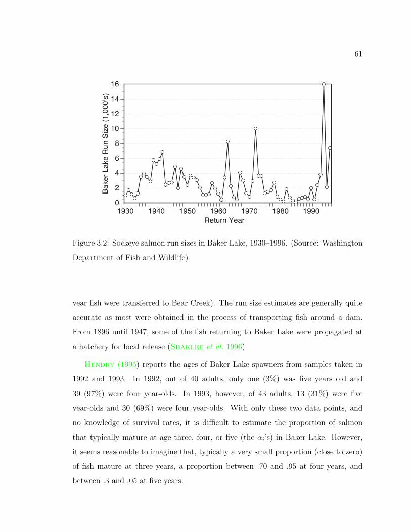
61

1930 1940 1950 1960 1970 1980 19900

2

4

6

8

10

12

14

16

Bake

r Lak

e Ru

n Si

ze (1

,000

's)

Return Year

Figure 3.2: Sockeye salmon run sizes in Baker Lake, 1930–1996. (Source: Washington

Department of Fish and Wildlife)

year fish were transferred to Bear Creek). The run size estimates are generally quite

accurate as most were obtained in the process of transporting fish around a dam.

From 1896 until 1947, some of the fish returning to Baker Lake were propagated at

a hatchery for local release (Shaklee et al. 1996)

Hendry (1995) reports the ages of Baker Lake spawners from samples taken in

1992 and 1993. In 1992, out of 40 adults, only one (3%) was five years old and

39 (97%) were four year-olds. In 1993, however, of 43 adults, 13 (31%) were five

year-olds and 30 (69%) were four year-olds. With only these two data points, and

no knowledge of survival rates, it is di#cult to estimate the proportion of salmon

that typically mature at age three, four, or five (the #i’s) in Baker Lake. However,

it seems reasonable to imagine that, typically a very small proportion (close to zero)

of fish mature at three years, a proportion between .70 and .95 at four years, and

between .3 and .05 at five years.

62

I simulated genetic drift in a model Baker Lake population with a number of

di!erent maturity schedules from “greatly overlapping” (#3 = 13 , #4 = 1

3 , #5 = 13),

to “barely overlapping” (#3 = 0, #4 = .95, #5 = .05). Each such maturity schedule

gives its own “average generation length”—between 3.8 years and 4.3 years for the

maturity schedules I simulated from. For each maturity schedule I initialized the

allele frequency in the spawners of years 1932 to 1936 to the same value (.1, .2, . . . , .9,

over di!erent simulations), then, starting at year 1937 I drew 2Ns new gene copies by

the scheme described above, to produce the spawners in that year. This was repeated

for 1938, ‘39, ‘40, and so on until obtaining an allele frequency at year 1993. This

whole process was repeated 20,000 times for each starting frequency, and the variance

of simulated allele frequencies in 1993 computed.1 This variance then translates (by

solving for N in Equation 2.7) into an e!ective size defined to be the size of a Wright-

Fisher population with a generation length equal to the average generation length for

the maturity schedule being simulated that would give the same increase in variance

of gene frequency in 56 years.

I used two di!erent values for Ns/Ni, the number of e!ective spawners per fish

counted in the run-size data. In one simulation I took Ns to be 0.16 of the number

of spawners counted by WDF&W, and in a second simulation I chose Ns/Ni = 0.32.

I chose the low value of 0.16 because some of the fish counted at the dam trap on

Baker Lake fail to reach the spawning grounds. The simulations using .16 should

be fairly conservative (i.e., they ought not result in an overestimate of the e!ective

population size) and the simulations that use 0.32 should provide a good “middle-

ground” estimate of the e!ective size.

The results of the simulations are shown for Ns/Ni = 0.16 [Figure 3.3(a)], and

1 In retrospect, I could have taken the simulated gene frequencies from both 1992 and 1993 (the

years that Hendry et al. collected samples from Baker Lake) and used both to estimate the

variance of the drift component of error in the samples. Note that using 1993 is conservative; it

will generally result in a low Ne because of the low returns in 1989, 1985, and 1981.

63

Ns/Ni = .32 [Figure 3.3(b)]. As one would expect, those maturity schedules with

more overlap yield higher e!ective sizes (the separate year classes are closer to being

one, larger, well-mixed population). A maturity schedule between 0/.8/.2 and 0/.9/.1

is probably close to that of Baker Lake sockeye. Thus our “low” estimate of Baker

Lake’s historical e!ective size over the time period of interest is about 250 individuals

drifting for 14 generations. A non-conservative estimate is about 600 individuals.

(An additional item we learn from these simulations is that the result is not

sensitive to the initial allele frequency. This is to be expected since the p(1# p) term

is included in the expression for variance (2.7). For future simulations, though, we

may simulate from only a few initial allele frequencies, knowing that our results are

still general.)

3.2.2 Simulations for Cultus Lake

The historical census records for Cultus Lake are also very good. The escapement

estimates for the years 1942–1993 are shown in Figure 3.4. From the return years

1953 to the present, estimates of the age composition of the returning fish are also

available. Of all returning fish over that time period, 2% were estimated to be three

year-olds, 95% four year-olds, and 3% five year-olds.

Since fish planted into North Creek in 1944 would have been the o!spring of fish

returning to Cultus Lake in 1943, ideally we could find age and escapement data for

the years 1938 to the present. However such data are not available, so I filled in the

holes as follows: 1) from 1938 to 1941 I took the escapement to be the harmonic mean

of the escapement for the years 1943 to 1953, with age composition being .02/.95/.03;

2) for 1942 to 1945 the escapement data are available but I had to assume an age

composition of .02/.95/.03 in each return year; 3) though age data are not available

for the years 1946–1952, I used the scheme described for Baker Lake to determine

the number of three-, four- and five year-olds in each of those return years (again,

assuming an age composition of .02/.95/.03. For the years 1952 to 1992, escapement

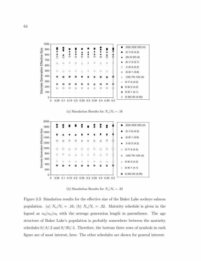
64

0

100

200

300

400

500

600

700

800

900

1000

0 0.05 0.1 0.15 0.2 0.25 0.3 0.35 0.4 0.45 0.5

Disc

rete

Gen

erat

ion

Effe

ctive

Size

.333/.333/.333 (4)

.3/.1/.6 (4.3)

.25/.5/.25 (4)

.6/.1/.3 (3.7)

.1/.6/.3 (4.2)

.3/.6/.1 (3.8)

.125/.75/.125 (4)

0/.7/.3 (4.3)

0/.8/.2 (4.2)

0/.9/.1 (4.1)

0/.95/.05 (4.05)

(a) Simulation Results for Ns/Ni = .16

0

200

400

600

800

1000

1200

1400

1600

1800

2000

0 0.05 0.1 0.15 0.2 0.25 0.3 0.35 0.4 0.45 0.5

Disc

rete

Gen

erat

ion

Effe

ctive

Size

.333/.333/.333 (4)

.3/.1/.6 (4.3)

.3/.6/.1 (3.8)

.1/.6/.3 (4.2)

0/.7/.3 (4.3)

.125/.75/.125 (4)

0/.8/.2 (4.2)

0/.9/.1 (4.1)

0/.95/.05 (4.05)

(b) Simulation Results for Ns/Ni = .32

Figure 3.3: Simulation results for the e!ective size of the Baker Lake sockeye salmon

population. (a) Ns/Ni = .16, (b) Ns/Ni = .32. Maturity schedule is given in the

legend as #3/#4/#5 with the average generation length in parentheses. The age

structure of Baker Lake’s population is probably somewhere between the maturity

schedules 0/.8/.2 and 0/.95/.5. Therefore, the bottom three rows of symbols in each

figure are of most interest, here. The other schedules are shown for general interest.

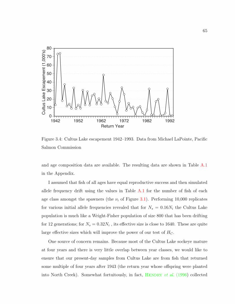
65

1942 1952 1962 1972 1982 19920

10

20

30

40

50

60

70

80Cu

ltus

Lake

Esc

apem

ent (

1,00

0's)

Return Year

Figure 3.4: Cultus Lake escapement 1942–1993. Data from Michael LaPointe, Pacific

Salmon Commission

and age composition data are available. The resulting data are shown in Table A.1

in the Appendix.

I assumed that fish of all ages have equal reproductive success and then simulated

allele frequency drift using the values in Table A.1 for the number of fish of each

age class amongst the spawners (the $i of Figure 3.1). Performing 10,000 replicates

for various initial allele frequencies revealed that for Ns = 0.16Ni the Cultus Lake

population is much like a Wright-Fisher population of size 800 that has been drifting

for 12 generations; for Ns = 0.32Ni , its e!ective size is close to 1640. These are quite

large e!ective sizes which will improve the power of our test of HC .

One source of concern remains. Because most of the Cultus Lake sockeye mature

at four years and there is very little overlap between year classes, we would like to

ensure that our present-day samples from Cultus Lake are from fish that returned

some multiple of four years after 1943 (the return year whose o!spring were planted

into North Creek). Somewhat fortuitously, in fact, Hendry et al. (1996) collected

66

juveniles in 1992 that were o!spring of the return year 1991, which is on the proper

four year cycle (1943, 1947,. . . , 1987, 1991).

3.2.3 Simulations for Bear Creek

It is much more di#cult to determine the e!ective size of the Bear Creek population

since 1937 because there is little census data. WDF&W has records for Bear Creek

only since 1982, so it may be impossible to get a good estimate of Bear Creek’s

historical e!ective size. I have, however, considered a biologically plausible scenario

under which Bear Creek’s e!ective size would be about 100. Ultimately one has to

decide if that seems reasonable or not given only scarce historical data. Nonetheless,

I shall carry out the tests for a Bear Creek Ne of 100 as this is as small as possible

without risking breakdown of the asymptotic approximations upon which many of

the expressions for " in Chapter 2 are based.

For Bear Creek, I performed simulations following the scheme used for Baker Lake,

assuming Ns = .25Ni. I used a single maturity schedule (#3 = .125, #4 = .75, and

#5 = .125) which is close to the average age composition of Bear Creek sockeye that

Hendry and Quinn (1997) report from two years of data. To obtain run sizes for

1932–1981, I imagined that the Bear Creek population was of size 25 individuals in

1932 and then grew by the equation

Nyear = 25 + 17, 161*

year# 1932

1982# 1932

+6

. (3.1)

Such a 6th degree polynomial relationship gives a population growth curve that starts

slowly, and then “rushes up” to meet the population size of 17,186 in 1982 (the open

triangles in Figure 3.5). This is a growth pattern that coincides temporally with

the increase of sockeye in Lake Washington in the late 1960’s (Edmondson 1991).

In other words, it assumes that the Bear Creek population was very small until

only recently. Simulating over 10,000 replicates with the values from (3.1) yields an

historical e!ective size of 116.

67

1932 1942 1952 1962 1972 1982 19920

5

10

15

20

25

30

Bear

Cre

ek R

un S

ize (1

,000

's)

Return Year

Known Data

Polynomial (Deterministic)

Polynomial (Stochastic)

Figure 3.5: Yearly run sizes for Bear Creek for the purposes of genetic drift simula-

tions. Filled circles are WDF&W estimates. Polynomial (Deterministic) are values

obtained from Equation 3.1 and Polynomial (Stochastic) are one set of realized values

from Equation 3.2. Notice how this assumes that the Bear Creek population was very

small for many years, and the rapid growth of the population starting in the 1960’s,

mirrors the remarkable growth of other Lake Washington populations at the same

time (Kolb 1971; Edmondson 1991).

68

Salmon run sizes, however, seldom follow a smooth curve through time like the

one determined by (3.1). Accordingly, I repeated the simulations several times for

run sizes determined each year by

Nstoch =

<=>

=?

y if y > 0

12 if y $ 0(3.2)

where y is the realized value of a normal random variable with mean equal to Nyear

as determined by (3.1) and variance equal to (Nyear/2.5)2 (i.e., coe#cient of variation

equal to 40%). The open diamonds in Figure 3.5 show one realization of run sizes.

Over several simulations using run sizes generated by the random model of (3.2) the

e!ective size was around 105. This says that even if there were some early years when

very few (say 10 or 12) fish returned to Bear Creek, the e!ective size could still be

close to 100 because the population has grown to be quite sizeable today.

Additional complexity Unfortunately there is a further complication. The histor-

ical e!ective size just given for Bear Creek assumed that the number of spawners in

each of the the years from 1932 to the present was a realization from Equation 3.2.

This might be reasonable if the Bear Creek population were already established be-

fore the introductions from Baker Lake. However if HA is true, then the Bear Creek

population would have started with only a single year class. In e!ect, under HA, the

adults “returning” to Bear Creek in 1936 were Baker Lake adults spawned at the

Birdsview Hatchery whose fry were released into Lake Washington. Since almost 2.5

million fry raised from these adults were released to various Lake Washington locales

(see Table 1.1) there was clearly a great number of adults contributing to fry released

to Bear Creek—likely at least 800 females, assuming the average female had 2,900

eggs, as suggested by Royal and Seymour (1940). Considering that the number of

males spawned may not have been as great, we might make a conservative estimate

that there were 100 “e!ective” Baker Lake adults in 1936 that contributed fry to

Bear Creek. Subsequently, there should have been zero fish returning in 1937 and

69

Table 3.2: An example of Bear Creek run-size history under HA that gives an histor-ical e!ective size of about 100 under simulations as described on Page 66. The first15 years follow a distinct pattern of strong and weak returns as might be expecteddue to the initial stocking from Baker Lake taking place in only one year. For 1950to 1981 the runs sizes are a realization of Equation 3.2, and from 1982 to 1993 theyare estimates from WDF&W data.1937 0 1952 156 1967 2,568 1982 17,8711938 0 1953 140 1968 2,153 1983 20,7201939 6 1954 231 1969 2,023 1984 21,3351940 50 1955 163 1970 1,595 1985 20,1601941 10 1956 155 1971 6,497 1986 22,9821942 0 1957 534 1972 4,618 1987 18,8441943 8 1958 263 1973 7,830 1988 8,7791944 60 1959 580 1974 3,887 1989 1,7951945 30 1960 94 1975 9,707 1990 10,1151946 10 1961 254 1976 9,535 1991 7,6911947 16 1962 664 1977 19,372 1992 27,5331948 80 1963 1,558 1978 10,428 1993 9,8481949 66 1964 1,781 1979 14,7971950 27 1965 2,811 1980 13,8681951 65 1966 2,576 1981 15,231

1938, very few, if any, in 1939, some four year-olds in 1940 and a few five year-olds in

1941, and then again, not many more fish until 1944 and 1945. Under this scenario,

there are fewer fish overall and so the e!ective size will be smaller. In particular, for

the historical e!ective size of the Bear Creek population to be as large as 100, then

there must have been more than 25 fish returning in 1940. A scenario which gives an

e!ective size of about 100 is that of starting with 100 “e!ective spawners” in 1936,

and then having the returns listed in Table 3.2.

A number of simulations verified that the run sizes which would most influence

the e!ective size of the population over the last fifty-six years under this model of

population growth, are precisely the earliest ones (for example 1940 and 1944) about

which little is known. There is one relevant report, though: Royal and Seymour

(1940) write that no fish were observed in the creek in September of 1940, but in

70

October, two were counted over a rack installed by the State Game Deptartment.

Unfortunately there is no indication of how much e!ort went into the surveys or

whether the rack was positioned so as to intercept every fish entering Bear Creek and

its tributaries. We are left wondering if as many as 50 fish might have entered the

Bear Creek system in 1940 without being caught in the rack.

3.2.4 On the shapes of the distributions

In the above three subsections, I’ve defined historical e!ective sizes in terms of the

increase in allele frequency variance over time. However, it remains to be shown

whether a gene drifting in a population with overlapping year classes will have the

same t-generation probability distribution as a gene drifting in an appropriately-sized

Wright Fisher population without overlapping generations. When the probability

of allele fixation is small (and such cases are the ones we limit ourselves to) the

two distributions appear to be very similar. Figure 3.6(a) shows a Monte Carlo

approximation to the allele frequency distribution for a Bear Creek population with

run sizes as in Table 3.2. These simulations revealed a final allele frequency variance

comparable to that of a Wright-Fisher population of 103 individuals drifting for 14

generations. A Monte Carlo approximation to the distribution of allele frequency

in such a Wright-Fisher population after 14 generations appears in Figure 3.6(b).

Evidently the Wright-Fisher model of the appropriate size is a suitable approximation.

3.3 Computing Likelihood Ratios for HA

Under HA, the hypothesis that the Bear Creek population descended exclusively from

fish planted from Baker Lake, we can compute a " for each of the four loci separately

and then add them all together for our final test statistic which will have a chi-square

distribution on four (or five, see below) degrees of freedom. We thus get to choose the

71

0 0.1 0.2 0.3 0.4 0.5 0.6 0.7 0.8 0.9 10

0.01

0.02

0.03

0.04

Prop

ortio

n of

50,

000

Repl

icate

s

Ending Frequency

(a) Overlapping Year Classes

0 0.1 0.2 0.3 0.4 0.5 0.6 0.7 0.8 0.9 10

0.01

0.02

0.03

0.04

Prop

ortio

n of

50,

000

Repl

icate

s

Ending Frequency

(b) Wright Fisher Population

Figure 3.6: Simulation results showing that an appropriately-sized Wright-Fisher

population is a good approximation for a population with overlapping year classes.

(a) The result of 50,000 replicates of drift in a model Bear Creek population with

overlapping year classes and run sizes as given in Table 3.2. (b) Simulation results

for an appropriately sized Wright-Fisher population drifting for 14 generations. Each

simulation used .3 as the initial allele frequency. The two distributions are clearly

very similar.

72

best method from Chapter 2 for each locus. (“Best” here means a su#ciently accurate

method that requires the least computation.) In computing the test statistics for HA,

the time t was taken as 14 generations (i.e., [1993#1936]÷4 years average generation

length is about 14).

Computing " for PGM–2* is the easiest of the four. Its two alleles are codom-

inant, and the *136 allele appears in the samples from Baker and from Bear at

frequencies of .142 and .140 respectively. The maximum likelihood estimate of the

starting frequency p of *136 under all hypotheses is then going to be no less than

.140. Returning to Figure 2.8 on Page 40, we see that for populations of N * 100,

the probability of an allele starting at .14 drifting to fixation in 14 generations is very

small. Hence, the normal approximation to drift transition probabilities will hold,

and we can very quickly obtain " from Equation 2.31. Appendix B.1 shows an input

file to Mathematica that will compute this quantity.

Dealing with ALAT* is more complicated. Since there are three codominant

alleles at the locus, we must use the density in the stereographically projected space

(Equation 2.30 gives the log of that density) to compute the density for our sample

and hence to find ". However, the frequency of the *95 allele in the sample from Baker

Lake is .06. The maximum likelihood estimate (using the normal approximations that

we do here) of the original frequency of *95 in Baker Lake is thus .06. Consulting

Figure 2.8 again, we see that such a starting frequency will result in fixation > 6%

of the time in a population of size N $ 200. Consequently, when computing " for

instances when we take the e!ective size of Baker Lake to be less than Ne ! 300, we

must lump the *95 allele with *91 or *100 and treat the two as one, computing " as

for PGM–2*. (The same is true if we take Bear Creek to have an e!ective size less

than ! 250.) This lumping throws away information, and one must be wary because

lumping *95 with *91 will result in a smaller " than will lumping *95 with *100.

I have chosen to always lump in the conservative direction, such that it will yield a

smaller ". Appendix B.2 shows some input to Mathematica that will compute " for

73

a triallelic locus using the coordinates in the stereographically projected space.

For PGM–1*, which includes the recessive *NULL allele, we use the sample den-

sity for recessive alleles developed in Section 2.8.1. (See Appendix B.3 for some

Mathematica input.)

Finally, dealing with the LDH–A1* locus is the most di#cult, because it involves

a recessive allele that was not detected in any samples from Baker Lake. Under the

hypothesis of separate origin, the maximum likelihood estimate of the frequency of the

recessive *500 in 1936 in Baker Lake is zero, and the probability of the sample given

p = 0 is clearly 1. This is a probability mass, and so we need a sample mass method

to compute ". (I tried various sample density methods, including the sample density

for recessive alleles, and they did not perform well.) The Angular approximation

sample mass method for recessive alleles (Equation 2.33) works well. The frequency

of the *500 is high enough in Bear Creek that the maximum likelihood estimate

of its frequency in 1936 under the hypothesis of common origin (HA) is generally

higher than .1 (at least while assuming Bear Creek e!ective population sizes that

are not very, very small) and the probability of fixation in 14 generations for an

allele starting at frequency greater than .1 for a population of N > 100 is reasonably

low. So, likelihoods for LDH–A1* computed using (2.33) should be quite accurate.

Computing " by this method requires much more computer time than for the other

methods. Appendix B.4 shows a Mathematica input for computing this likelihood

ratio.

3.4 Computing Likelihood Ratios for HC

For HC , similarly, we must choose how to compute " for the di!erent loci. We

can compute " for PGM–2* and LDH–A1* in the same way we did for HA. For

PGM–1* as well, we can use the sample density for recessive alleles developed in

Section 2.8.1, but only because the e!ective size of Cultus Lake has been so large

74

that the probability that an allele at frequency .962 (the maximum likelihood estimate

of the initial frequency of *Null under the alternative hypothesis) drifts to fixation

(frequency 1.0) is small. Finally, since the *95 allele does not appear in the sample

from Cultus Lake, we must treat ALAT* as a diallelic locus, lumping *95 with *100

to be conservative. And here, even though the mle of the initial frequency of *91 in

Cultus Lake under the alternative hypothesis is .05, the large e!ective size ensures

that the Angular method approximation will work well.

For testing HC , t is 12 generations, since the introduction from Cultus Lake

occurred eight years after the introduction from Baker Lake.

3.5 Testing the Cedar River

In order to assess how well the statistical method performs in a case where the null

hypothesis is known to be true, we may try to reject the hypothesis that the sockeye

in the Cedar River descended from the Baker Lake introductions (call that HR).

Since the Cedar River contained no lake-rearing habitat for juvenile sockeye before

it was diverted into Lake Washington, and because the only transplants made to the

Cedar were from Baker Lake (outside of any survivors of the Cultus transplants to

Issaquah Creek that might have later been transferred to the Cedar River when some

sockeye o!spring from the Issaquah Hatchery were planted into the Cedar River), the

Cedar River population is almost certainly from Baker Lake. Thus, we should fail to

reject HR for all reasonable e!ective sizes of the Cedar population. Carrying out this

test, I assumed that the Cedar population’s history up to 1993 could be adequately

represented by a Wright-Fisher population of size NR drifting for 14 generations, even

though some plantings from Baker Lake occurred as late as 1944. This is allowable

since t and N always occur together as t/N , in the transition densitities, so any

dicrepancy in t can is made up for by exploring di!erent values of N .

It is di#cult to determine an e!ective size for the Cedar River population. The

75

population was not consistently surveyed until 1967, shortly after it began growing

rapidly. In the ten years before 1993, the run size was never below 76,000 individuals

(Figure 1.2). However, in 1962, the run size estimate was as low as 2,100, and in 1961

it was 9,900 (Kolb 1971). In fact, Kolb (1971) states that the returns of sockeye to

Lake Washington “fluctuated at low levels after 1940 and general interest diminished

until. . . the early 1960’s”(p. 3). It is therefore unlikely that the run sizes to the Cedar

River were larger than a few thousands of fish each year before the mid-1960’s. In

Appendix A.2 I describe how I combined run size data from di!erent sources and

performed simulations to determine the approximate e!ective size of the Cedar River

population. These simulations suggest that if the annual escapement in the Cedar

River was 500 between 1940 and 1960, then its historical e!ective size would be about

1150 individuals. Likewise, if the run sizes were about 2,000 for each year between

1940 and 1960, the e!ective size would be 4,100. Even if there were as many as 5,000

fish every year between 1940 and 1960, the e!ective size of the Cedar River would

only be about 9,000.

Hendry et al. (1996)’s data for the Cedar river is shown in Table 3.3. To compute

" with these values, and the large e!ective sizes that we will be assuming, we can use

the normal-based approximations for three loci: for PGM–2*, the standard Angular

method; for ALAT*, the density for three alleles in the stereographically projected

space (so long as Baker’s e!ective size is taken to be greater than 300); and for

PGM–1*, the sample density method for null alleles. Using the data from LDH–A1*

is more di#cult. Since the observed frequency in the Cedar sample is so low, the mle

of the frequency of the *500 allele in Baker Lake under the null hypothesis would be

very small, and it would not be possible to accurately obtain a probability mass for

the sample due to the high probability of fixation. However, we may assume that for

LDH–A1* the e!ective sizes in Baker Lake and the Cedar River have been infinite, so

that the frequency of *500 does not change due to genetic drift, and the di!erences in

observed frequencies arise only from sampling. Such an assumption gives a larger "

76

Table 3.3: Sample allele frequencies from Hendry et al. (1996) at four loci in the

Cedar River. n is the sample size in number of diploid individuals for each locus.

The frequency of the alternate (*100) allele at each locus is not listed, but is 1 minus

the sum of the frequencies of the other alleles at the locus. POOLED DATA are the

allele frequency estimates after pooling the data between years. COUNT DATA are

the actual counts, x, of codominant alleles out of 2n gene copies, or the counts, y, of

recessive homozygote phenotypes out of n individuals in the pooled samples.

ALAT* PGM–1* PGM–2* LDH–A1*

Popln. Year n *91 *95 n *NULL n *136 n *500

Cedar 1992 76 0.382 0.072 40 0.447 134 0.086 135 0.086

1993 115 0.361 0.074 40 0.354 115 0.096 117 0.000

+ POOLED DATA +

Cedar 92,93 191 0.369 0.073 80 0.403 249 0.090 252 0.063

+ COUNT DATA +

Popln. Year 2n *91 *95 n *NULL 2n *136 n *500

Cedar 92,93 382 141 28 80 13 498 45 252 1

77

which is acceptable since the burden, in this case, is to demonstrate that the test does

not reject HR. Since the di!erences in the samples for LDH–A1* are only zero *500

homozygotes out of 120 individuals (Baker) against one homozygous individual out

of 252 (Cedar), there really is very little di!erence between them. Nonetheless, given

some initial frequency p of *500, the probability of finding y homozygotes in a sample

of size n can be obtained quickly by the poisson approximation to the binomial, i.e.,

if X % Bin(n, p) with pn ! 1 then X is distributed approximately Poisson(np).

Thus, denoting the sample sizes for LDH–A1* from Baker and Cedar to be nA

and nR, respectively, the joint probability of getting yA and yR recessive homozygotes,

given initial allele frequencies of pA and pR respectively is-

e"nApA(nApA)yA

yA!

. -e"nRpR(nRpR)yR

yR!

.

. (3.3)

Since yA = 0 and yR = 1, this reduces to nRpR exp{#(nApA + nRpR)}. When pA and

pR are not constrained to equal one another, this quantity is maximized when pA = 0

and pR = 1/nR, and it takes the value e"1. This is the numerator of our likelihood

ratio. When pA = pR = p (as under the null hypothesis) the likelihood can be

maximized by setting the first derivative w.r.t. p to zero. This gives the denominator

of the likelihood ratio: e"1nR/(nA + nR). And so, for testing HR we approximate "

for LDH–A1* as

"LDH"A1 = 2 log*

nA + nR

nR

+= 2 log

*120 + 252

252

+= 0.779. (3.4)

3.6 Results of the Likelihood Ratio Tests

3.6.1 Result for HA

The likelihood ratio test described above shows that it is unlikely that the sockeye in

Bear Creek could have descended exclusively from the Baker Lake plantings. Table 3.4

shows values of "j for each locus, and gives an overall (sum over loci) " with a

corresponding p-value for Bear Creek e!ective sizes of 75, 100, and 150, and several

78

Baker Lake e!ective sizes from 250 to 600 (which are our conservative and “middle

ground” estimates, respectively, from the historical population data). From the table

we see that if the e!ective size of Baker Lake were 250, and that of Bear Creek, 100,

then our probability of Type I error in rejecting HA would still be as low as .07.

(There are some caveats in interpreting these p-values explained in the Discussion.)

As can be seen from the di!erences in p-values for NB = 75, 100, and 150, the

result is sensitive to the value one is willing to accept for the e!ective size of the

Bear Creek population. I have included the results for NB = 75 to demonstrate this

sensitivity even though the result is likely to be somewhat inaccurate in this case

because of the non-negligible probability of allele fixation for alleles starting from a

frequency of about .15 (i.e., *96 at PGM–2* and *500 at LDH–A1* under the null

hypothesis).

An important feature of these results is that the overall test statistic does not rely

exclusively on a large contribution from LDH–A1*. The genetic di!erences between

Baker Lake and Bear Creek at PGM–1* also contribute substantially to our ability

to reject HA.

3.6.2 Result for HC

Table 3.5 gives values for the "j and p-values for the test of whether the Bear Creek

population could have descended exclusively from the plants from Cultus Lake. The

results are for Bear Creek e!ective sizes of 75, 100, and 150, and for one value of

e!ective size for Cultus Lake, 800, our conservative, low estimate of its historical

e!ective size for the last twelve generations. With such low p-values, it is even more

clear in this case that we may reject HC with very low probability of being incorrect

in doing so. This accords well with historical knowledge, as there is no record that

Cultus sockeye were ever planted directly into the Bear Creek system, but only to

other nearby tributaries of the Sammamish River or Lake Sammamish.

79

Table 3.4: Values of " at each locus for testing HA, assuming di!erent e!ective sizes

for Baker Lake and Bear Creek. NA is the e!ective size used for Baker Lake and NB

is for Bear Creek. In each of the next four columns are the test statistics computed

for the indicated loci computed as described in Section 3.3.!

"j gives the sum of the

individual test statistics as per Equation 2.5. The degrees of freedom for comparing

the test statistic to a %2 random variable are in the df column. For the e!ective sizes

considered, the degrees of freedom is 4 (one for each locus) because the three alleles

of ALAT* were lumped into two. The p-value is Pr(%24 *

!"j).

NA NB ALAT* PGM–1* PGM–2* LDH–A1*!

"j df p-value

250 75 1.103 2.737 0.000 3.589 7.430 4 0.114849

250 100 1.344 3.268 0.000 4.049 8.661 4 0.070159

250 150 1.718 4.082 0.000 4.678 10.478 4 0.033096

300 75 1.144 2.826 0.000 3.607 7.578 4 0.108325

300 100 1.405 3.398 0.000 4.091 8.894 4 0.063804

300 150 1.819 4.291 0.000 4.760 10.870 4 0.028066

400 75 1.200 2.947 0.000 3.628 7.775 4 0.100182

400 100 1.490 3.578 0.000 4.143 9.211 4 0.056039

400 150 1.964 4.586 0.000 4.868 11.418 4 0.022250

500 75 1.236 3.026 0.000 3.638 7.900 4 0.095326

500 100 1.546 3.697 0.000 4.173 9.416 4 0.051500

500 150 2.063 4.785 0.000 4.935 11.783 4 0.019041

600 75 1.261 3.081 0.000 3.643 7.986 4 0.092109

600 100 1.585 3.782 0.000 4.192 9.560 4 0.048534

600 150 2.134 4.928 0.000 4.981 12.044 4 0.017029

80

Table 3.5: Values of " at each locus for testing HC , assuming di!erent e!ective sizes

for Cultus Lake and Bear Creek. NC is the e!ective size used for Cultus Lake and NB

is for Bear Creek. In each of the next four columns are the test statistics computed

for the indicated loci computed as described in Section 3.4.!

"j gives the sum of the

individual test statistics as per Equation 2.5. The degrees of freedom for comparing

the test statistic to a %2 random variable are in the df column. For the e!ective sizes

considered, the degrees of freedom is 4 (one for each locus) because the three alleles

of ALAT* were lumped into two. The p-value is Pr(%24 *

!"j).

NC NB ALAT* PGM–1* PGM–2* LDH–A1*!

"j df p-value

800 75 5.933 9.120 0.090 3.032 18.174 4 0.001141

800 100 7.362 10.292 0.112 3.412 21.178 4 0.000292

800 150 9.696 11.899 0.147 3.932 25.675 4 0.000037

3.6.3 Result for HR: Making sure this test doesn’t reject everything

We test HR, the hypothesis that the Cedar River sockeye came exclusively from Baker

Lake, as a sort of “test of our hypothesis test.” It provides a general check on the test,

and, more importantly, gives us some information about the values used for e!ective

sizes of the populations involved. I have conducted the test for five values of Baker

Lake e!ective size from 250 to 600, and for values of the Cedar population’s historical

e!ective size of 1,200, 5,000, and 10,000. The results appear in Table 3.6, where it is

clear that we would not be able to reject HR “at the .05 level” even if we assumed

that the e!ective size of Baker Lake has been as high as 600 and of the Cedar River

as high as 10,000 since the 1930’s.

One di#culty with the above analysis, however, is that it may be preferable to ex-

clude LDH-A1* from the analysis, because variation at that locus between the Cedar

River and Baker Lake is so di#cult to detect. Such a change, however, alters the

results very little. Note that if we drop LDH-A1* from the analysis and compare the

81

Table 3.6: Values of " at each locus for testing HR, assuming di!erent e!ective sizes

for Baker Lake and the Cedar River. NA is the e!ective size used for Baker Lake

and NR is for the Cedar River population. In each of the next four columns are the

test statistics computed for the indicated loci computed as described in Section 3.5.

The value in the LDH–A1* column is the likelihood ratio for that locus assuming

infinite Cedar and Baker population sizes (explained in Section 3.5).!

"j gives the

sum of the individual test statistics as per Equation 2.5. The degrees of freedom for

comparing the test statistic to a %2 random variable are in the df column. For the

e!ective sizes considered, the degrees of freedom is five—two for ALAT* and one for

the each of the other loci because the three alleles of ALAT* need not be lumped

into two. The p-value is Pr(%24 *

!"j).

NA NR ALAT* PGM–1* PGM–2* LDH–A1*!

"j df p-value

250 1,200 2.987 0.190 0.649 0.779 4.605 5 0.46591

250 5,000 3.281 0.210 0.730 0.779 5.000 5 0.41593

250 10,000 3.399 0.213 0.745 0.779 5.136 5 0.39953

300 1,200 3.420 0.202 0.735 0.779 5.136 5 0.39953

300 5,000 3.714 0.225 0.840 0.779 5.558 5 0.35166

300 10,000 3.832 0.229 0.860 0.779 5.699 5 0.33658

400 1,200 4.202 0.221 0.880 0.779 6.082 5 0.29833

400 5,000 4.496 0.249 1.036 0.779 6.559 5 0.25553

400 10,000 4.614 0.254 1.065 0.779 6.712 5 0.24293

500 1,200 4.890 0.235 0.998 0.779 6.902 5 0.22803

500 5,000 5.183 0.267 1.204 0.779 7.433 5 0.19035

500 10,000 5.302 0.273 1.244 0.779 7.598 5 0.17985

600 1,200 5.500 0.245 1.097 0.779 7.621 5 0.17841

600 1,500 5.542 0.254 1.154 0.779 7.729 5 0.17182

600 5,000 5.793 0.281 1.349 0.779 8.203 5 0.14539

600 10,000 5.911 0.288 1.400 0.779 8.379 5 0.13656

82

resulting!

"j to a chi-square distribution on four degrees of freedom (four because

we lose one degree of freedom when we eliminate the LDH–A1* locus) the result is

very similar. In fact, the resulting p-values are never more than .036 less than those

reported in Table 3.6. Thus, the lowest p-value, that for NA = 600 and NR = 10, 000

is .10738.

Such a p-value of .10738 does appear disturbingly low, however, and this probably

indicates that an estimate of 600 for Baker Lake’s e!ective size is too high, and that

our lower bound estimate of 250 is much closer to the true value of Baker Lake’s

e!ective size than the non-conservative estimate derived earlier to be 600. Assuming

NA = 250 and NR = 10,000 yields a p-value of .39.

3.7 Discussion

This final section recaps several features of the likelihood-ratio test and discusses

its applicability to other instances of inference on the ancestral origin of introduced

populations. It then describes issues in the interpretation of the p-values from the

test and o!ers several conclusions about the Bear Creek sockeye and the information

available in genetic data for inferring their ancestral origin. Finally, I o!er some

suggestions for future work, both statistical and empirical, on the origin of Bear

Creek sockeye.

3.7.1 The test and other applications

The test presented here is a generalized likelihood ratio test—a commonly employed

method of testing hypotheses. The main di#culty in conducting the test is computing

the likelihoods. The methods I used to do so were similar to those used in admixture

analyses by Thompson (1973) and Long (1991). They both (either explicitly or

implicitly) expressed their likelihood as a probability density for their samples.

One of the conspicuous features of the Bear Creek problem was the moderate

83

frequency of the *500 allele of LDH–A1* in Bear Creek, and its absence in samples

from Baker and Cultus lakes. This required a novel treatment because of the break-

down of the asymptotic approximations with allele frequencies equal to or near zero.

It was necessary to compute probability masses for the samples under HA and HC

and the general alternative hypotheses corresponding to each. Numerically integrat-

ing the binomial sampling probabilities weighted by the appropriate drift transition

probabilities (as in Equation 2.33) worked well for this. However, it was quite for-

tunate that conditions were such that the method worked. Had there been just one

homozygous *500 individual in the sample from Baker Lake then (2.33) would not

have properly computed the probability mass for that sample under the hypothesis of

separate origin. (Since there were, in actuality, no *500 homozygotes in the sample it

was easy to compute its probability mass given the most likely initial gene frequency;

it was simply unity.) A truly general method would require a di!erent approach to

approximating probability masses for samples—one which is still accurate when the

probability of allele fixation is non-negligible.

The test requires much information to bound its assumptions regarding historical

e!ective population size. Additionally, since it seeks to say something about the ori-

gin of a population by rejecting putative donor populations, the test demands good

information about which populations may be donors. It is thus not clear that this

test is widely applicable to other problems of inferring the origin of recently estab-

lished populations. I have identified six recent studies which used genetic analyses

to infer the origin of introduced organisms. Hattemer and Ziehe (1996) describe

an approach that is similar to the approach taken here, in that they attempted to

exclude the possibility that a stand of oddly-shaped beech trees, Fagus sylvatica L.,

originated from any of 22 stands of trees in the Rheinland-Pfalz region of Germany.

They did not take a strict hypothesis-testing approach, but they do acknowledge that

any inferences they could make were complicated by genetic drift. Unlike the Bear

Creek problem, though, they had to contend with the fact that some of their enzyme

84

markers are well known to experience selective pressures in di!erent environments.

For that reason, the test I have proposed would not be suitable for their problem.

Kambhampati et al. (1991) studied allozyme frequencies in 57 populations of

the Asian-native mosquito Aedes albopictus from four di!erent continents. They

used both genetic distance analysis and a discriminant analysis to conclude that A.

albopictus populations in the U.S. and Brazil probably originated from Japan. They

note that fixation of some alleles in the Brazilian population suggests a “founder

e!ect” but do not address how that might a!ect the confidence in their conclusions

about the origin of the Brazilian mosquito populations. Roehner et al. (1996)

studied the distribution of allele frequencies in polychaete populations, concluding

that recently established populations in Europe’s North and Baltic Seas originated

from the eastern seaboard of the U.S. They based their conclusions on Nei’s genetic

distance measure (Nei 1978), and they proposed that genetic drift was likely not an

important factor because the population transfers typically involve large numbers of

individuals carried in the ballast water of ocean-going ships. Morrison and Scott

(1996) studied the origin of an exotic weed in Australia by allozyme electrophoresis

of samples from 54 populations worldwide. Applying the likelihood ratio test of

Chapter 2 to the situations studied in any of these three papers would be di#cult.

E!ective sizes are known even less accurately than they are in Lake Washington, and

the issue of multiple comparisons would be problematic because there is not a small

set of possible donor populations.

Mendel et al. (1994) used randomly-amplified, polymorphic DNA (RAPD) mark-

ers to determine the origin of a scale insect pest in Israel. RAPD’s do not lend them-

selves to analyses which assume Mendelian inheritance. Finally, Kriegler et al.

(1995) used allozyme frequencies to classify 38 Tennessee populations of brook trout,

Salvelinus fontinalis, as being either of hatchery origin, wild origin, or both. They

based their classifications on a system devised by McCracken et al. (1993) which

relies on the fixation of alternate alleles at some loci between hatchery and wild fish. If

85

researchers wanted to test hypotheses about the origin of particular brook trout pop-

ulations, the hypothesis test I have presented, since it relies on approximations that

are typically inaccurate in the face of allele fixation, would probably have di#culty

handling all of the data of Kriegler et al. (1995).

3.7.2 Interpretation of p-values

The hypothesis test here requires a number of assumptions, many of which were

mentioned in Section 2.10. The heaviest requirement is the assumption that the

historical e!ective sizes of the populations in the test are known without error. If

there is some probability that the estimates of Ne used are incorrect, then, of course,

the p-value will not accurately reflect the probability of Type I error. I have tried

to manage this by choosing Ne’s for the populations in question that are probably

lower than the true Ne’s. It is reasonable to think that this has been accomplished

for the Baker and Cultus Lake populations by choosing low values of Nb/Ni (Page 62)

and ages at maturity that o!ered little overlap between years, and by using the good

run-size data for the two populations.

I cannot say the same for my estimates of Ne for Bear Creek. I provided an

example of the sorts of run sizes in the early 1940’s to the early 1980’s that would

lead to genetic drift comparable to that in a population of Ne = 100 for 14 generations,

but accurate run-size data for Bear Creek in the years before 1982 do not exist. It is

important to realize that the results of the tests presented here are highly dependent

on the e!ective sizes chosen, and, conspicuously, since Bear Creek’s population size

has likely been smaller than the others’, it is Bear Creek’s size to which the tests are

most sensitive. In a sense, it seems that framing the origin of Bear Creek sockeye

in a hypothesis-testing framework has replaced “global ignorance,” an inability to

statistically assess the origin of the Bear Creek fish because we didn’t know how to

do so, with “local ignorance,” i.e., we know what to do but one piece of the puzzle

is missing entirely—knowledge of Bear Creek’s historical run sizes. Yet, by casting

86

the problem in a statistical framework, we have learned a good deal about what

knowledge is required to assess inferences in this sort of problem.

Two other important considerations in interpreting our p-values are the related is-

sues of ascertainment and multiple comparisons. The multiple-testing problem arises

because we have performed three separate tests (one for each of HA, HC , and HR),

and thus the p-value for any one of the tests reflects not only the Type I error proba-

bility for that test, but also the fact that we have “given ourselves three chances” to

obtain a p-value below any given level.

The ascertainment problem2 arises because the population in Bear Creek was

singled out from the surveys of Hendry et al. (1996) and Seeb and Wishard (1977)

as having allele frequencies di!erent from those in the three other sockeye populations

in Lake Washington and the two putative donor stocks. The problem here may be

seen by a simple analogy. Suppose that you wished to test whether a coin was fair

(had equal probability of coming up heads or tails) so you flipped it 10,000 times in

sets of ten. At the end of that, suppose you noticed that in one of the sets of ten flips

the coin came up heads every time. If you based your test on this one set of ten heads

without considering that it was only one set of 1,000, you could overwhelmingly reject

the hypothesis that the coin was fair, but doing so would obviously be incorrect. The

situation in testing HA and HC with Bear Creek is similar, yet more intricate since

we know a priori that some of the populations (e.g., Cedar River) very likely had no

spawning sockeye before the plantings from Baker Lake.

One way to treat both the multiple-testing and ascertainment problems would

be to use a Bonferroni correction. That is, in order to reject any hypothesis at a

prescribed #-level we would require the p-value to be # divided by the number of

comparisions we’ve made (which would be three for the various hypothesis tests,

plus two more for looking at the allele frequencies in Issaquah Creek and the beach

2 I thank Warwick Daw in the Department of Statistics for first pointing this out to me.

87

spawning population, as well). Doing this, however, would make the test excessively

conservative, as the Bonferroni correction is a conservative tool. Since the test is

already based on conservative assumptions of no migration between Lake Washington

stocks (Section 2.10), lower bound estimates of Ne for Baker and Cultus Lakes, and

lumping alleles in the conservative direction (Page 72), it might be desirable to simply

allow those conservative assumptions to be, in e!ect, a correction for the multiple

testing and the ascertainment of the Bear Creek sample (Elizabeth Thompson

University of Washington, Department of Statistics, pers. comm.).

The final act in interpreting a p-value may be using it to help make a decision. One

decision that awaits making is whether the Bear Creek population will be changed

from Provisional ESU status to ESU status, thus allowing its listing, if necessary,

under the Endangered Species Act (ESA), or to non-ESU status, in which case it

could not be listed under the ESA (Gustafson et al. 1997). In light of this, I o!er

two important considerations.

First, the notion of declaring some statistical test “significant” only if it gives a

p-value below some previously-determined value (for instance, .05), has fallen into

disfavor among many statisticians and fisheries managers (Pat Sullivan, Interna-

tional Pacific Halibut Commission, P.O. Box 95009, Seattle, WA 98145). For this

reason, I have provided the actual p-values from the hypothesis test under di!erent

assumptions about e!ective size. It would be unwise to disregard a p-value of, say,

.07 or .08, for rejecting HA, simply because it is greater than the “traditional” .05

level.

Second, any decision-making process which uses statistical significance levels must

also consider the Type II error rate of the test; that is, the probability of failure to

reject the null hypothesis when it is false. Typically the Type II error rate of a test

is explored by considering the power of the test (one minus the Type II error rate)

to reject the null hypothesis when it is false to some specified degree. The issue of

statistical power is particularly important in those cases when the p-values from a test

88

are not very low. The Bear Creek situation is one such example, and the assumption

of low e!ective size reduces the statistical power.

I have not undertaken a formal power analysis, but a simple analogy makes clear

how low the power in this test is. Imagine that you are trying to carry out some

sort of contingency-table test for genetic di!erences between two salmon populations,

i.e., you are conducting a simple G-test, say, to determine if two populations have

significantly di!erent allele frequencies at the time of sampling. Then, the sample

sizes which would give you statistical power comparable to the test I have presented

with NB = 100 and NA = 250 would be about n = 7 fish for the sample from one

population and n = 18 for the other sample.3 Very few people would give much

weight to a “non-significant” result from samples of size n = 7 and n = 18. And,

likewise, failure to reject HA while assuming small e!ective sizes would constitute

extremely weak grounds for believing that the sockeye in Bear Creek descended from

the Baker Lake transplants.

3.7.3 Conclusions on Bear Creek

If we accept that Bear Creek’s historical e!ective size was 100, and if we agree to

our conservative estimate of a Baker Lake e!ective size of 250 individuals, then we

may conclude from the data of Hendry et al. (1996) that Bear Creek sockeye could

not be exclusively derived from the Baker Lake plantings at the p = .07 level. This

demonstrates that the observed allele frequencies in Bear Creek are very di!erent

from those in Baker Lake. For comparison, using the same e!ective size (250) for

Baker Lake and assuming an extremely generous Cedar River historical e!ective size

of 10,000, we would not reject the hypothesis that the Cedar population derived

exclusively from Baker Lake (p = .39).

3 These values may be approximately derived by finding the binomial sample size n such that if

X % Bin(2n, p) and if sin"1;

X/(2n) D#& N(sin"1)p, 1/(8n)), then 1/(8n) will be equal to the

variance of " (see Page 29) which is at least t/(8NB) (or t/(8NA)).

89

We can be even more confident in rejecting the hypothesis that Bear Creek’s

population descended entirely from Cultus Lake. If we assume an e!ective size of 75

from Bear Creek and use our conservative estimate of 800 for Cultus’ e!ective size,

we reject HC with p = .001. This p-value may be slightly high due to the possibility

of allele fixation (see, for example, Figure 2.13), but the di!erence will be slight, and

our conclusion the same: there is substantial evidence against an exclusive Cultus

Lake origin.

We must consider these results in light of Royal and Seymour (1940)’s obser-

vation that the State Dept. of Game captured only two fish in Bear Creek in 1940

(the year the most adults should have been returning from the 1937 releases of Baker

Lake fry to Bear Creek). If the Game Dept. was really set up to intercept most of the

fish entering Bear Creek, then probably fewer than 50 fish returned in 1940 and the

historical e!ective size of Bear Creek’s population would likely be less than 100 due

to this extreme founder e!ect. As the statistical test shows, we cannot say as much

from the data of Hendry et al. (1996) if this is the case.

The goal of my analysis has not only been to test HA and HC , but also to assess

how much information regarding those hypotheses may be found in present-day allele-

frequency data. In this regard, the analysis has been successful. I have presented

a method which makes explicit what must be known if one wishes to statistically

characterize the strengths of their conclusions regarding the origin of Bear Creek

sockeye. The result that the power of Hendry et al. (1996)’s data to reject HA

depends heavily on unknown run sizes, though disapointing, is not unexpected. The

awareness that founder e!ects are bound to a!ect inferences such as these is not at

all new, however, the likelihood ratio test provides a way to judge the magnitude of

such e!ects.

90

3.7.4 Future work on Bear Creek

Further statistical analysis. The above method, relying as it does on the Brownian

motion approximation to genetic drift transition probabilities, has been taken up to

its limit. In order to extend the statistical analysis so it may accurately handle smaller

assumed e!ective sizes and the inclusion of data from other datasets, and so as to

address the question of whether the sockeye of Bear Creek may have arisen from a

mixture of Baker and Cultus Lake transplants, it will be necessary to adopt a very

di!erent approach—one which dispenses with the Brownian motion approximation,

and instead determines probabilities or test statistics and their distributions entirely

by computer simulation.

The first application for such a method should be to use the additional informa-

tion available in other allele-frequency datasets. For example, including the data of

Seeb and Wishard (1977) from Bear Creek, Baker Lake, and Cultus Lake would

be valuable. Though the sample sizes of Seeb and Wishard (1977) are not as large

as those of Hendry et al. (1996), they collected their data from Baker Lake at a

time when considerably less genetic drift had occurred in the population since the

1930’s, so their data are potentially quite informative. From a statistical standpoint,

an interesting challenge in using both datasets comes from the fact that the data

of Hendry et al. (1996) is not independent of the observations made by Seeb and

Wishard, because they are connected in time to one another via a stochastic pro-

cess. Thus, deriving the joint probability for the two sets of data would require some

care.

There have also been other, more recent, collections of fish from Baker Lake

(Winans et al. 1996; Shaklee et al. 1996) which ought to be included in the anal-

ysis. Including them in the current analysis is di#cult because the increased data at

LDH–A1* in Baker Lake makes the maximum likelihood estimate of the frequency of

the *500 allele under the null hypothesis, HA, low enough that the normal approxi-

91

mation is no longer accurate. Preliminary work suggests that including such data will

only strengthen the case against HA or HC . When a good computational method for

hypothesis testing is developed and used with these other datasets I expect to observe

lower p-values than obtained here, and to be able to reject HA, even while assuming

that the historical e!ective size of the Bear Creek population is considerably less than

100 individuals.

A computational approach would also lend itself more readily to testing whether

Bear Creek sockeye may have descended from a mixture of Baker Lake and Cultus

Lake transplants. I have not addressed such a “mixture hypothesis” in this thesis,

though I have elsewhere investigated a possible method for testing it. As is apparent

from Table 3.1, the allele frequencies of the *91 allele at ALAT* and the *NULL

allele at PGM–1* in Bear Creek are intermediate to the frequencies in Baker and

Cultus Lake. Accordingly (and this is also borne out in practice) contributions to

the likelihood ratio statistic for testing the mixture hypothesis come primarily from

LDH–A1*. Since no LDH–A1* *500 homozygotes have been reported from any

samples from Baker and Cultus lakes, one possibly fruitful, and relatively simple

first step would be to estimate, by Monte Carlo simulation, the joint probability of

finding no *500 homozygotes in the samples from Baker and Cultus lakes, and the

observed number (or more) of *500 homozygotes in the samples from Bear Creek,

given some initial frequencies of the *500 allele in Baker and Cultus lakes at the time

of the introductions. If this joint probability were very low for all di!erent initial

frequencies of the allele in Baker and Cultus lakes, this could be taken as evidence

against the mixture hypothesis. Some adjustment for the fact that LDH–A1* was

only one of several loci assayed would probably be appropriate.

Further empirical work Especially given the importance of the LDH–A1* *500

allele, as I discussed above, some recent developments indicate that more empiri-

cal work could be helpful. In particular, some parties have proposed that sockeye

92

from other sources have been introduced into Lake Washington. In October of 1997,

Andrew Hendry received an email message which read:

. . . also, I KNOW, that Kamchatka Sockeye WERE possibly planted

to Lake Washington in the late 60’s. I raised them from eggs shipped

here, and I know that the person who was supposed to have destroyed

them (200,000), later claimed that he didn’t (he is now deceased). JM

This assertion is made particularly interesting by the fact that Kamchatka is a region

where the *500 allele at LDH–A1* has been detected in anadromous sockeye popula-

tions (Paul Aebersold, NMFS Northwest Fisheries Science Center, pers. comm.).

Furthermore, the allele frequencies at PGM–1*, PGM–2*, and ALAT* of sockeye in

the Kamchatka River are quite close to those in Bear Creek (Varnavskaya et al.

1994). I believe this issue warrants further study, especially since the possibility of a

Kamchatka origin could be elegantly and simply tested with molecular markers.

Knowing little more than that some fish from somewhere in Kamchatka may

have been released into Lake Washington, hypothesis testing on the basis of allozyme

frequencies is an inappropriate tool for exploring this hypothesis. Varnavskaya

et al. (1994) list the allele frequencies of many sockeye populations in Kamchatka,

and some of them are very likely to have allele frequencies close to those in Bear

Creek. As mentioned above, the test I have proposed requires that one have a clear

idea of which populations may have been donors. It is not intended for surveying

many populations and finding one that has allele frequencies similar to those in Bear

Creek.

Instead, mitochondrial DNA should be useful in testing the Kamchatka hypoth-

esis. Bickham et al. (1995) surveyed sequences from the cytochrome b region of

mitochondrial DNA from sockeye salmon in North America and Asia. They found

that sockeye in the Fraser River, postglacially recolonized by fish from the “Columbia”

glacial refuge (Taylor et al. 1996), have a high (40%) frequency of an “AC” hap-

93

lotype that does not occur in populations from Kamchatka. The Fraser populations

do not possess the “GC” haplotype which occurrs in the Kamchatka populations at

a frequency of 50%. Since Baker Lake (and Lake Washington) were both ancestrally

recolonized by fish from the Columbia refuge, any stocks of native or Baker Lake

origin in Lake Washington should have a high frequency of “AC” and a low (or zero)

frequency of the “GC” haplotype. If a high frequency of “GC” were found in Bear

Creek, but in no other populations of sockeye in Washington and the Fraser River,

then that would provide good evidence that the sockeye in Bear Creek may have

come from Kamchatka. Such information, as well as other data collected in the fu-

ture on Lake Washington sockeye, should continue to clarify the issue of ancestry of

the sockeye in Bear Creek.

BIBLIOGRAPHY

Ajwani, S., 1956 A review of the Lake Washington watershed, historical, biolog-

ical and limnological. Master’s thesis, University of Washington. 3

Allendorf, F. W. and G. H. Thorgaard, 1984 Tetraploidy and the evolution

of salmonid fishes. In B. J. Turner (Ed.), Evolutionary Genetics of Fishes, pp.

1–53. New York: Plenum Press. 54

Bartley, D., M. Bagley, G. Gall, and B. Bentley, 1992 Use of linkage

disequilibrium data to estimate the e!ective size of hatchery and natural fish

populations. Conservation Biology 6: 365–375. 23

Bickham, J. W., C. C. Wood, and J. C. Patton, 1995 Biogeographic im-

plications of cytochrome b sequences and allozymes in sockeye salmon (On-

corhynchus nerka). J. Heredity 86: 140–144.

Burgner, R. L., 1991 Life history of sockeye salmon (Oncorhynchus nerka).

In C. Groot and L. Margolis (Eds.), Pacific Salmon Life Histories, pp. 1–117.

Vancouver: UBC Press. 58, 60

Cavalli-Sforza, L. L. and A. W. F. Edwards, 1967 Phylogenetic analysis:

models and estimation procedures. Evolution 21: 550–570. 38

Chrzatowski, M., 1983 Historical changes to Lake Washington and route of

the Lake Washington Ship Canal, King County, Washington. Accompaniment

to Water Resources Investigation Open-File Report 81–1182, United States

Geological Survey. 3

Cobb, J. N., 1927 Preliminary report of fishway work. Transactions of the Amer-

95

ican Fisheries Society 57: 181–201. 4

Crow, J. F. and C. Denniston, 1988 Inbreeding and variance e!ective numbers.

Evolution 42: 482–495.

Diggle, P. J. and R. J. Gratton, 1984 Monte Carlo methods of inference for

implicit statistical models (with discussion). Journal of the Royal Statistical

Society, Series B 46: 193–227. 34

Edmondson, W. T., 1991 The Uses of Ecology: Lake Washington and Beyond.

Seattle: University of Washington Press. 3, 66, 67

Edmondson, W. T., 1994 Sixty years of Lake Washington: A curriculum vitae.

Lake And Reservoir Management 10: 75–84.

Edwards, A. W. F., 1971 Distances between populations on the basis of gene

frequencies. Biometrics 27: 873–81.

Edwards, A. W. F., 1992 Likelihood. Baltimore: The Johns Hopkins University

Press. 18

Evermann, B. W. and E. L. Goldsborough, 1907 The fishes of Alaska.

Bulletin of the U.S. Fisheries Commision 26: 219–360. 4

Felsenstein, J., 1985 Phylogenies from gene frequencies: a statistical problem.

Systematic Zoology 34: 300–311.

Felsenstein, J., 1995 Theoretical Evolutionary Genetics. Seattle: ASUW Pub-

lications. 22, 25

Fisher, R. A., 1930 The Genetical Theory of Natural Selection. Oxford: Claren-

don Press. 15

Foote, C., G. S. Brown, and C. C. Wood, 1997 Spawning success of males

using alternative mating tactics in sockeye salmon, Oncorhynchus nerka. Cana-

dian Journal of Fisheries and Aquatic Sciences 54: 1785–1795.

96

Geyer, C. J., 1996 Estimation and optimization of functions. In W. R. Gilks,

S. Richardson, and D. J. Spiegelhalter (Eds.), Markov Chain Monte Carlo in

Practice, pp. 241–258. New York: Chapman and Hall. 35

Griffiths, R. C., 1979 A transition density expansion for a multi-allele di!usion

model. Advances in Applied Probability 11: 310–325. 27

Gustafson, R. G., T. C. Wainwright, G. A. Winans, F. W. Waknitz,

L. T. Parker, and R. S. Waples, 1997 Status review of sockeye salmon from

Washington and Oregon. U.S. Dept. Commer., NOAA Tech. Memo. NMFS–

NWFSC–33, 282 p. 1, 87

Hanson, A. J. and H. D. Smith, 1967 Mate selection in a population of sock-

eye salmon (Oncorhynchus nerka). Journal of the Fisheries Research Board of

Canada 24: 1955–1977. 60

Hattemer, H. H. and M. Ziehe, 1996 An attempt to infer on the origin of a

beech (Fagus sylvatica L.) stand in Rheinland-Pfalz (Germany). Silvae Genet-

ica 45: 276–283. 10

Hendry, A., 1995 Sockeye salmon (Oncorhynchus nerka) in Lake Washington:

an investigation of ancestral origins, population di!erentiation and local adap-

tation. Master’s thesis, University of Washington. 6, 56

Hendry, A. P. and T. P. Quinn, 1997 Variation in adult life history and

morphology among Lake Washington sockeye salmon (Oncorhynchus nerka)

populations in relation to habitat features and ancestral a#nities. Canadian

Journal of Fisheries and Aquatic Sciences 54: 75–84.

Hendry, A. P., T. P. Quinn, and F. M. Utter, 1996 Genetic evidence

for the persistence and divergence of native and introduced sockeye salmon

(Oncorhynchus nerka) within Lake Washington. Canadian Journal of Fisheries

and Aquatic Sciences 53: 823–832. 1, 4, 5, 10, 62

97

Jorde, P. E. and N. Ryman, 1995 Temporal allele frequency change and estima-

tion of e!ective size in populations with overlapping generations. Genetics 139:

1077–1090.

Kambhampati, S., W. C. I. Black, and K. S. Rai, 1991 Geographic origin

of the USA and Brazilian Aedes albopictus inferred from allozyme analysis.

Heredity 67: 85–94. 10

Karlin, S. A. and H. M. Taylor, 1975 A First Course in Stochastic Processes,

2nd Ed. New York: Academic Press. 24

Kendall, M. and A. Stuart, 1979 The Advanced Theory of Statistics, Vol. 2.

New York: Macmillan. 19, 50

Kimura, M., 1955a Random genetic drift in multi-allelic locus. Evolution 9:

419–435.

Kimura, M., 1955b Solution of a process of random genetic drift with a continuous

model. Proceedings of the National Academy of Sciences, USA 41: 144–150.

Kimura, M., 1956 Random genetic drift in a tri-allelic locus: exact solution with

a continuous model. Biometrics 12: 57–66.

Kolb, R., 1971 A review of Lake Washington sockeye (Oncorhynchus nerka) age

and racial characteristics as determined by scale pattern analysis. Supplemen-

tal progess report marine fisheries investigations, Washington Department of

Fisheries. 4, 67, 75

Kriegler, F. J., G. F. McCracken, J. W. Habera, and R. J. Strange,

1995 Genetic characterization of Tennessee brook trout populations and asso-

ciated management implications. North American Journal Of Fisheries Man-

agement 15: 804–813. 10

Krimbas, C. B. and S. Tsakas, 1971 The genetics of Dacus oleae. V. Changes

98

of esterase polymorphism in a natural population following insecticide control—

selection or drift? Evolution 25: 454–460.

Littler, R. A. and E. D. Fackerell, 1975 Transition densities for neutral

allele di!usion models. Biometrics 31: 117–123. 27

Long, J. C., 1991 The genetic structure of admixed populations. Genetics 127:

417–428. 45

McCart, P., 1970 A polymorphic population of Oncorhynchus nerka at Babine

Lake, B.C. involving anadromous (sockeye) and non-anadromous (kokanee)

forms. Ph. D. thesis, University of British Columbia, Vancouver. 55

McCracken, G. F., P. C. R, and S. Z. Guffey, 1993 Genetic di!erenti-

ation and hybridzation between hatchery stock and native brook trout in the

Great Smoky Mountains National Park. Transactions of the American Fisheries

Society 122: 533–542.

Mendel, Z., D. Nestel, and R. Gafny, 1994 Examination of the origin of the

Israeli population of Matsucoccus josephi (Homoptera: Matsucoccidae) using

random amplified polymorphic DNA-polymerase chain reaction method. Annals

Of The Entomological Society Of America 87: 165–169. 10

Morrison, S. M. and J. K. Scott, 1996 Variation of populations of Tribu-

lus terrestris (Zygophyllaceae): 3. Isozyme analysis. Australian Journal Of

Botany 44: 201–212. 10

Nei, 1978 Estimation of average heterozygosity and genetic distance from a small

number of individuals. Genetics 89: 583–590. 9, 84

Nei, M., 1987 Genetic distance and molecular phylogeny. In N. Ryman and F. M.

Utter (Eds.), Population Genetics and Fishery Management, pp. 21–46. Seattle:

University of Washington Press. 54

99

Nei, M. and F. Tajima, 1981 Genetic drift and estimation of e!ective population

size. Genetics 98: 625–640. 23

Ostergaard, E., 1995 Status report: Abundance of spawning kokanee in the

Sammamish River basin. Addendum to 1994 status report. Technical report,

King County Surface Water Management. 5

Pamilo, P. and S. Varvio-Aho, 1980 Letter to the editor of the estimation of

population size from allele frequency changes. Genetics 95: 1055–1058. 23

Pfeifer, B., 1992 Fisheries Investigations of Lakes Washington and Sammam-

ish—1980–1990. Part V. Wild cutthroat and kokanee in Lakes Washington and

Sammamish. Technical report, Washington Department of Fisheries. Unpubl.

Draft. 4

Pollak, E., 1983 A new method for estimating the e!ective population size from

allele frequency changes. Genetics 104: 531–548. 23

Roehner, M., R. Bastrop, and K. Juerss, 1996 Colonization of Europe by

two American genetic types or species of the genus Marenzelleria (Polychaeta:

Spionidae). An electrophoretic analysis of allozymes. Marine Biology 127: 277–

287. 10

Rounsefell, G. A. and G. B. Kelez, 1938 The salmon and salmon fisheries of

Swiftsure Bank, Puget Sound, and the Fraser River. Bulletin of the U.S. Bureau

of Fisheries 49: 693–823. 4

Royal, L. A. and A. Seymour, 1940 Building new salmon runs. Progressive

Fish Culturist 52: 1–7. 5, 6

Seeb, J. and L. Wishard, 1977 The use of biochemical genetics in the man-

agement of Pacific salmon stocks: genetic marking and mixed fishery analysis.

Final Report Service Contract 792, Washington Department of Fisheries. 1, 90

100

Shaklee, J. B., J. Ames, and L. LaVoy, 1996 Genetic diversity units and

major ancestral lineages for sockeye salmon in Washington. Technical Report

RAD 95–02, Washington Department of Fish and Wildlife. 9, 61, 90

Sokal, R. R. and F. J. Rohlf, 1981 Biometry, 2nd ed. New York: W. H.

Freeman and Company. 19

State of Washington Department of Fisheries and Game, 1919b Fifth and sixth

annual reports of the state game warden to the to the Governor of the State of

Washington March 1, 1917 to February 28, 1917. Wash. Dept. of Fish. Game,

Olympia, WA.

State of Washington Department of Fisheries and Game, 1932a Fortieth and forty-

first annual reports of State Department of Fisheries and Game, Division of

Fisheries, for the period from April 1, 1929, to March 31, 1931. Wash. Dept. of

Fish. Game, Olympia, WA. 4

State of Washington Department of Fisheries and Puget Sound Treaty Indian

Tribes Northwest Indian Fisheries Commission, 1992 Puget Sound sockeye

salmon forecasts and management recommendations. Olympia, WA. 103

Taylor, E. B., C. J. Foote, and C. C. Wood, 1996 Molecular genetic evidence

for parallel life-history evolution within a Pacific salmon (sockeye salmon and

kokanee, Oncorhynchus nerka). Evolution 50: 401–416. 92

Thompson, E. A., 1972 The likelihood for multinomial proportions under stere-

ographic projection. Biometrics 28: 618–620.

Thompson, E. A., 1973 The Icelandic mixture problem. Annals of Human Ge-

netics, London 37: 69–80. 45

Utter, F. M., P. Aebersold, and G. Winans, 1987 Interpreting genetic

variation detected by electrophoresis. In N. Ryman and F. M. Utter (Eds.),

101

Population Genetics and Fishery Management, pp. 21–46. Seattle: University

of Washington Press. 10, 54

Varnavskaya, N. V., C. C. Wood, and R. J. Everett, 1994 Genetic vari-

ation in sockeye salmon (Oncorhynchus nerka) populations of Asia and North

America. Canadian Journal of Fisheries and Aquatic Sciences 51(Suppl. 1):

132–146. 92

Waples, R. S., 1989 A generalized approach for esimating e!ective population

size from temporal changes in allele frequency. Genetics 121: 379–391.

Waples, R. S., 1990 Conservation genetics of Pacific salmon: III. Estimating

e!ective population size. Journal of Heredity 81: 277–289. 58

Waples, R. S., 1995 Evolutionarily Significant Units and the conservation of

biological diversity under the Endangered Species Act. In J. L. Nielsen (Ed.),

Evolution and the Aquatic Ecosystem: defining unique units in population con-

servation, pp. 8–27. Bethesda, MD: American Fisheries Society Symposium 17.

14

Waples, R. S., O. W. Johnson, P. B. Aebersold, C. K. Shiflett, D. M.

VanDoornik, D. J. Teel, and A. E. Cook, 1993 A genetic monitoring and

evaluation program for supplemented populations of salmon and steelhead in

the Snake River basin. Annual report of research, Coastal Zone and Estuarine

Studies Division, Northwest Fisheries Science Center, National Marine Fisheries

Service, NOAA. 58

Winans, G. A., P. B. Aebersold, and R. S. Waples, 1996 Allozyme variabil-

ity of Oncorhynchus nerka in the Pacific Northwest, with special consideration

to populations of Redfish Lake, Idaho. Transactions of the American Fisheries

Society 125: 645–663. 90

Wood, C. C., B. E. Riddell, D. T. Rutherford, and R. E. Withler,

102

1994 Biochemical genetic survey of sockeye salmon (Oncorhynchus nerka) in

Canada. Canadian Journal of Fisheries and Aquatic Sciences 51(Suppl. 1):

114–131. 10, 55, 55

Woodey, J. C., 1966 Sockeye spawning grounds and adult returns in the Lake

Washington watershed, 1965. Master’s thesis, University of Washington. 6

Wright, S., 1931 Evolution in Mendelian populations. Genetics 16: 97–159.

Zar, J. H., 1984 Biostatistical Analysis, 2nd ed. Englewood Cli!s, NJ: Prentice

Hall. 19

Appendix A

DETERMINING THE EFFECTIVE SIZES

A.1 Population Sizes and Age Composition of Cultus Lake Sockeye

A.2 Determining E!ective Size of the Cedar River Population

To compute an e!ective size for the Cedar River population I gathered population

size estimates from various sources. Escapement estimates for 1961–1969 come from

Kolb (1971). For 1970 to 1991 there are sockeye counts from the H. M. Chittenden

Locks (State of Washington Department of Fisheries and Puget Sound Treaty Indian

Tribes Northwest Indian Fisheries Commission 1992) For the years 1982 to 1993,

Ron Egan of the Washington Department of Fish and Wildlife provided me with

Cedar River escapement data. The Cedar escapement is lower than the counts at

the Locks because of prespawning mortality and the fact that the fish ascending the

ladders at the locks are a mixture of fish from all the di!erent populations in Lake

Washington, not just the Cedar River. For the period 1982–1991, on average, the

Cedar escapement was 78 percent of the counts at the Locks. Therefore, I obtained

rough escapement estimates for 1970–1981 by multiplying the counts at the Locks by

Table does not appear here because it is a longtable and apparently

not compatible with the current hyperref implentation in Textures.

If you really want to see this table you can obtain my thesis from

the University of Washington

Table A.1: The table that does not appear here

104

0.78.

The run-size data for 1970–1991 do include estimates of age composition. These

age class counts are for a mixture of all the Lake Washington populations, so they

are not entirely representative of the Cedar River population. (In particular there

are probably relatively more three year-olds among the mixed group of returning fish

than in the Cedar River.) Nonetheless, they are a good approximation. The average

proportion of di!erent-aged fish in Lake Washington from 1970 to 1991 was 12% three

year-olds, 85% four year-olds, and 3% five year-olds. For the years 1970–1991 I took

the number of fish of each age class in the Cedar River to be .78 of the number of

fish counted at the locks in that age class. For 1932–1969 I took the proportion of

three year olds to be .12 of the total escapement; the proportion of four year-olds to

be .85; and the proportion of five year-olds to be .03. For 1992 and 1993, I used the

age compositions of Cedar River samples reported by Hendry and Quinn (1997).

We don’t know how large the Cedar River population was before 1960. Kolb

(1971) says it was small. I performed four di!erent simulations, each time assuming

that the escapement was of constant size Nu in each year before 1960. Such a scheme

leads to the population numbers shown in Table A.2 which I used in the simulations.

I ran simulations for four di!erent values of Nu: 500, 1,000, 2,000, and 5,000.

105

Table A.2: Cedar River escapements used in the simulations to determine e!ectivesize.

Return Year 3 yr-olds 4 yr-olds 5 yr-olds Total1932 .12Nu .85Nu .03Nu Nu

......

......

...1960 .12Nu .85Nu .03Nu Nu

1961 1,188 8,415 396 9,9001962 252 1,785 84 2,1001963 4,236 30,005 1,412 35,3001964 8,220 58,225 2,740 68,5001965 5,760 40,800 1,920 48,0001966 5,448 38,590 1,816 45,4001967 2,273 16,099 758 18,9401968 19,200 136,000 6,400 160,0001969 14,880 105,400 4,960 124,0001970 32,794 133,708 8,507 105,7341971 15,862 676,793 25,430 433,8421972 26,613 340,997 18,840 233,4801973 24,689 557,989 4,651 354,8431974 29,958 178,461 9,415 131,6081975 17,969 157,831 9,448 111,9211976 18,738 188,551 24,142 139,8231977 4,185 729,986 20,604 456,0091978 5,052 392,719 3,084 242,1831979 6,043 256,663 32,980 178,6431980 27,796 609,726 2,378 386,6051981 57,314 89,495 6,680 92,7331982 2,839 244,048 6,772 253,6581983 64,867 125,919 2,551 193,3381984 55,600 279,945 1,415 336,9601985 49,044 168,928 5,773 223,7451986 37,914 176,411 2,808 217,1331987 60,076 114,360 3,405 177,8411988 32,867 325,556 576 359,0001989 103,489 57,935 576 162,0001990 23,540 51,452 1,008 76,0001991 14,165 61,544 1,291 77,0001992 0 94,000 6,000 100,0001993 760 47,120 28,120 76,000

Appendix B

ROUTINES FOR COMPUTING THE LIKELIHOOD

RATIO

Following are a series of sample inputs to Mathematica that I used to compute "

in various cases.

B.1 Diallelic Codominant Loci

I used the following input file to compute " for diallelic codominant loci such as

PGM–2* and for ALAT* when I had lumped the*91 allele together with one of the

other alleles, making it appear to be a diallelic locus.

(* This Mathematica input defines a function that computesthe likelihood ratio test statistic for a simple dialleliclocus with codominant alleles. It includes the data for‘‘b’’ = Bear Creek and ‘‘a’’ = Baker Lake at the PGM-2 locus.FUNCTION NAME:

‘‘LambdaEasy’’VARIABLES/INPUTS:

t ->time of drift in generationsna ->effective size of population Anb ->effective size of population Bsa -> size of sample from population A (# of individuals)sb -> size of sample from population B (# of individuals)xa -> allele count in sample Axb ->allele count in sample B

DATA VALUES FOR PGM--2: *) (t = 14;sb = 207;xb = 58;sa = 120;xa = 34;

(* FUNCTION DEFINITION *)

107

LambdaEasy[t_,na_,nb_,sa_,sb_,xa_,xb_] := N[( ArcSin[Sqrt[xa/(2sa)]] - ArcSin[Sqrt[xb/(2sb)]] ) ^2 /( t/(8na) + 1/(8sa) + t/(8nb) + 1/(8sb) ) ];

(* LOOP TO PRINT VALUES FOR DIFFERENT VALUES OF na AND nb *)size = {50,75,100,150,200,250,300,400,500,600,700,800,900,1000};For[i=1,i<=14,i++, na = size[[i]];

For[j=1,j<=14,j++, nb = size[[j]];PutAppend[{na, nb, LambdaEasy[t,na,nb,sa,sb,xa,xb]}, "pgm2out" ] ]

])

B.2 Triallelic Codominant Locus

For ALAT* with all three of its alleles, the functions defined in the following input

file compute " using the stereographic projection:

(* This Mathematica input defines a function that computesthe likelihood ratio test statistic for a trialleliclocus with codominant alleles, using the density from thestereographically projected space. (Actually it uses thelog-density the whole way through. It includes the data for‘‘b’’ = Bear Creek and ‘‘a’’ = Baker Lake at the ALAT locus.I’ve opted to use the sample gene frequencies rather than thecount data because the counts don’t appear anyhwere in the ex-pressions for this thing.FUNCTION NAME:‘‘LambdaFunct’’VARIABLES/INPUTS:

t ->time of drift in generationsna ->effective size of population Anb ->effective size of population Bsa -> size of sample from population A (# of individuals)sb -> size of sample from population B (# of individuals)freqa1 -> frequency of first allele in sample Afreqa2 -> frequency of second allele in sample Afreqa3 -> frequency of third allele in sample Afreqb1 -> frequency of first allele in sample Bfreqb2 -> frequency of second allele in sample Bfreqb3 -> frequency of third allele in sample B

DATA VALUES FOR ALAT: *) (t = 14;sa = 83;

108

sb = 163;freqa1 = .403;freqa2 = .537;freqa3 = .06;freqb1 = .598;freqb2 = .273;freqb3 = .129;

(* FUNCTION TO COMPUTE THE SUM IN THE TRANSFORMATION *)SumFre[f1_,f2_,f3_] := Sqrt[f1/3] + Sqrt[f2/3] + Sqrt[f3/3];

(* FUNCTION TO TRANSFORM VARIABLES INTO STER PROJ SPACERETURNS THEM IN A LIST *)ProjectFreq1[f1_,f2_,f3_] :=

N[( (2(Sqrt[f1] + Sqrt[1/3]) /(1 + SumFre[f1,f2,f3]) ) ) - Sqrt[1/3] ];

ProjectFreq2[f1_,f2_,f3_] :=N[( (2(Sqrt[f2] + Sqrt[1/3]) /(1 + SumFre[f1,f2,f3]) ) ) - Sqrt[1/3] ];

ProjectFreq3[f1_,f2_,f3_] :=N[( (2(Sqrt[f3] + Sqrt[1/3]) /(1 + SumFre[f1,f2,f3]) ) ) - Sqrt[1/3] ];

(* ASSIGN THE TRANSFORMED VALUES TO THE VARIABLES wa1,wa2, etc. *)wa1 = ProjectFreq1[freqa1,freqa2,freqa3];wa2 = ProjectFreq2[freqa1,freqa2,freqa3];wa3 = ProjectFreq3[freqa1,freqa2,freqa3];wb1 = ProjectFreq1[freqb1,freqb2,freqb3];wb2 = ProjectFreq2[freqb1,freqb2,freqb3];wb3 = ProjectFreq3[freqb1,freqb2,freqb3];

(* COMPUTE VARIANCES *)TheVar[n_,s_,t_] := N[ ( (t/(4n)) + (1/(4s)) ) ] ;vara = TheVar[na,sa,t];varb = TheVar[nb,sb,t];

(* MLE’S OF JOINT DISTRIBUTION ARE WEIGHTED AVERAGES *)p1 = ( varb * wa1 + vara * wb1 ) / (vara + varb);p2 = ( varb * wa2 + vara * wb2 ) / (vara + varb);p3 = ( varb * wa3 + vara * wb3 ) / (vara + varb);

(* COMPUTE LAMBDA *)LambdaFunct[wa1_,wa2_,wa3_,wb1_,wb2_,wb3_,p1_,p2_,p3_] := 2 * (

( ( (wa1 - p1)^2 + (wa2 - p2)^2 + (wa3 - p3)^2 ) /( (t/(4na)) + (1/(4sa)) ) ) + ( ( (wb1 - p1)^2 +(wb2 - p2)^2 + (wb3 - p3)^2 ) / ( (t/(4nb)) + (1/(4sb)) ) ) )

)(* COMPUTE FOR VARIOUS EFFECTIVE SIZES *)(size = {50,75,100,150,200,250,300,400,500,600,700,800,900,1000};

109

For[i=1,i<=14,i++, na = size[[i]];For[j=1,j<=14,j++, nb = size[[j]];PutAppend[{na, nb, LambdaFunct[wa1,wa2,wa3,wb1,wb2,wb3,p1,p2,p3]},"alat.sterout" ] ]

])

B.3 Diallelic Locus With Recessive—PGM–1*

For a locus such as PGM–1* which has a recessive allele that is detected in ample

numbers in both samples we may use the sample density method of Section 2.8.1.

(* This Mathematica input computesthe likelihood ratio test statistic for a dialleliclocus with one recessive allele that appears in bothof the samples (like the PGM-1 locus for Baker Lakeand Bear Creek). It uses the sample density methodfor null alleles, and this file includes the data for‘‘b’’ = Bear Creek and ‘‘a’’ = Baker Lake at the PGM-1 locusVARIABLES/INPUTS

t ->time of drift in generationsna ->effective size of population Anb ->effective size of population Bsa -> size of sample from population A (# of individuals)sb -> size of sample from population B (# of individuals)ya -> # of recessive homozygotes in sample Ayb -># of recessive homozygotes in sample Bp -> used by FindMinimum. It ends up being the

mle of the ancestral frequency under thehypothesis of common origin *)

(t = 14;sb = 160;yb = 68;sa = 79;ya = 10;numera = FindMinimum[-1 *

( 2*Pi*(t*p(1-p)/(2na) + (1-p^2)/(4sa) ) )^(-.5) *Exp[ (-(p - Sqrt[ya/sa])^2) /(2*(t*p(1-p)/(2na) + (1-p^2)/(4sa) ) ) ],{p, {.3,.305}} ];

numerb = FindMinimum[-1 *

110

( 2*Pi*(t*p(1-p)/(2nb) + (1-p^2)/(4sb) ) )^(-.5) *Exp[ (-(p - Sqrt[yb/sb])^2) /(2*(t*p(1-p)/(2nb) + (1-p^2)/(4sb) ) ) ],{p, {.6,.605}} ];

denom = FindMinimum[-1 *( 2*Pi*(t*p(1-p)/(2na) + (1-p^2)/(4sa) ) )^(-.5) *

Exp[ (-(p - Sqrt[ya/sa])^2) /(2*(t*p(1-p)/(2na) + (1-p^2)/(4sa) ) ) ] *

( 2*Pi*(t*p(1-p)/(2nb) + (1-p^2)/(4sb) ) )^(-.5) *Exp[ (-(p - Sqrt[yb/sb])^2) /(2*(t*p(1-p)/(2nb) + (1-p^2)/(4sb) ) ) ],

{p, {.5,.505}} ];loglr = 2*Log[ (numera[[1]] * numerb[[1]]) / (-1*denom[[1]])];PutAppend[{na,nb,loglr,denom[[2]]},"pgm1xtra"])

B.4 Diallelic Locus With Recessive—LDH–A1*

LDH–A1*, since it includes a recessive allele that was not detected in the samples

from Baker Lake or Cultus Lake requires special treatment. The following input

will compute " by the sample mass method for recessive alleles using the Angular

approximation.

(* This Mathematica input computesthe likelihood ratio test statistic for a dialleliclocus with one recessive allele that does not appear in oneof the samples (like the LDH-A1 locus). It includes the data for‘‘b’’ = Bear Creek and ‘‘a’’ = Baker Lake for the LDH-A1 locus.Note that the variables na and nb must be assigned values beforethis is run.VARIABLES/INPUTS

t ->time of drift in generationsna ->effective size of population Anb ->effective size of population Bsa -> size of sample from population A (# of individuals)sb -> size of sample from population B (# of individuals)sahomo -> # of recessive homozygotes in sample Asbhomo -># of recessive homozygotes in sample Bldhnullt -> used by FindMinimum. It ends up being the

mle of the ancestral frequency under the

111

hypothesis of common origin *)(t = 14;sb = 130;sbhomo = 8;sa = 120;sahomo = 0;ldha = 1 (* THE MAX OF THE LIKELIHOOD FUNCTION IS 1 *) ;ldhb = NIntegrate[ ( 2*Pi*(t/(8nb)) )^(-.5) *

Exp[-((x-ArcSin[Sqrt[ Sqrt[sbhomo/sb] ]])^2)/(t/(4nb))] *Binomial[sb,sbhomo] *((Sin[x])^(4*sbhomo)) *(1- ( (Sin[x])^4 ) )^(sb-sbhomo),{x, 0 ,Pi/2},WorkingPrecision->5 ] ;

ldht = FindMinimum[ -1*NIntegrate[ ( 2*Pi*(t/(8na)) )^(-.5) *

Exp[-((x-ArcSin[Sqrt[ldhnullt]])^2)/(t/(4na))] *Binomial[sa,sahomo] *((Sin[x])^(4*sahomo)) *(1- ( (Sin[x])^4 ) )^(sa-sahomo),{x, 0 ,Pi/2},WorkingPrecision->5 ] *

NIntegrate[ ( 2*Pi*(t/(8nb)) )^(-.5) *Exp[-((x-ArcSin[Sqrt[ldhnullt]])^2)/(t/(4nb))] *Binomial[sb,sbhomo] *((Sin[x])^(4*sbhomo)) *(1- ( (Sin[x])^4 ) )^(sb-sbhomo),{x, 0 ,Pi/2},WorkingPrecision->5 ] ,

{ldhnullt, {.1,.11}} ];ldhloglr = 2*Log[(ldha*ldhb)/(-1*ldht[[1]])];PutAppend[{na,nb,ldhloglr,ldht[[2]]}, "ldhnofunout" ])