0

NASA Contractor Report 201730

User’s Manual for FEMOM3DSVersion 1.0

C. J. ReddyHampton University, Hampton, Virginia

M. D. DeshpandeViGYAN,Inc., Hampton, Virginia

NASA Cooperative Agreement NCC1-231

August 1997

National Aeronautics andSpace AdministrationLangley Research CenterHampton, Virginia 23681-0001

1

CONTENTS

1. Introduction 2

2. Installation of the code 2

3. Operation of the code 4

4. Sample runs 8

5. Test Cases 16

6. Concluding Remarks 19

Acknowledgments 19

Appendix 1 Theory for FEMOM3DS 20

Appendix 2 Listing of the distribution disk 27

Appendix 3 Sample *.SES file of COSMOS/M 29

Appendix 4 Generic input file format for PRE_FEMOM3DS 31

References 33

2

1. INTRODUCTION

FEMOM3DS is a computer code written in FORTRAN 77 to compute

electromagnetic(EM) scattering characteristics of a three dimensional object with complex

materials (figure 1) using combined Finite Element Method (FEM)/Method of Moments

(MoM) technique[1]. This code uses the tetrahedral elements, with vector edge basis

functions for FEM in the volume of the cavity and the triangular elements with the basis

functions similar to that described in [2], for MoM at the outer boundary. By virtue of FEM,

this code can handle any arbitrarily shaped three-dimensional cavities filled with

inhomogeneous lossy materials. The basic theory implemented in the code is given in

Appendix 1.

The User’s Manual is written to make the user acquainted with the operation of the

code. The user is assumed to be familiar with the FORTRAN 77 language and the operating

environment of the computers on which the code is intended to run. The organization of the

manual is as follows. Section 1 is the introduction. Section 2 explains the installation

requirements. The operation of the code is given in detail in Section 3. Two example runs, the

first EM scattering characteristics of a dielectric sphere and the second EM scattering

characteristics form an inlet cavity are demonstrated in Section 4. Some test cases are

presented in Section 5 to show the flexibility of the code. The test cases were run by the

authors to validate the code. Users are encouraged to try these cases to get themselves

acquainted with the code.

2. INSTALLATION OF THE CODE

The distribution disk of FEMOM3DS is floppy disk formatted for IBM

compatible PCs. It contains a file namedfemom3ds.tar.gz . This file has to be transferred

to any UNIX machine viaftp using binary mode. On the UNIX machine, use the following

commands to get all the files.

gunzip femom3ds.tar.gz

tar -xvf femom3ds.tar

This creates a directoryFEMOM3DS-1.0, which in turn contains the

3.5''

3

So

Sb

n

Dielectric Scattererwith PEC bodies

Fictitious outer boundary

Figure 1 Illustration of the scattering body with surface, Sbenclosed by a fictitious outer surface So , which is usedto terminate the FEM compuatational domain.

εr1

µr1

εr2 εr3µr2

µr3

X

Z

Y

θ

φ

4

subdirectories, FEMOM3DS (source files for the main code),PRE_FEMOM3DS (source files

for preprocessing code),Example1 and Example2. As the code is written in

FORTRAN 77, with no particular computer in mind, the source code in these directories

should compile on any computer architecture without any problem. The code was

successfully complied on a CONVEX machine, and the compilation can be done by using a

makefile file for the different machines such as SUN, SGI etc. The complete listing of the

directories in the distribution disk is given in Appendix 2.

3.0 OPERATION OF THE CODE

The computation of EM scattering characteristics from a specific geometry with

FEMOM3DS is a multi-stage process as illustrated in figure 2. The geometry of the problem

has to be constructed with the help of any commercial Computer Aided Design (CAD)

package. In our case, we used COSMOS/M[3] as our geometry modeler and meshing tool.

Once the object geometry is modelled, PEC surfaces are to be identified for implementing

proper boundary conditions. As FEMOM3DS uses edge based basis functions, the nodal

information supplied by most of the meshing routines cannot be readily used. Hence, a

preprocessor PRE_FEMOM3DS is written to convert the nodal based data into edge based

data and then is given as input to FEMOM3DS. For the convenience of the users, who use

different CAD/meshing packages other than COSMOS/M, PRE_FEMOM3DS accepts the

nodal based data in a generic format also. The procedures involved for using COSMOS/M

input data file or generic input data file are explained below.

5

With the help of COSMOS/M, the geometry is constructed and meshed with

tetrahedral elements. The user is assumed to be familiar with COSMOS/M package and its

features. Once the mesh is generated, one needs to identify the following to impose proper

boundary conditions:

(a) tetrahedral elements with different material parameters1,

(b) elements on PEC surfaces

(c) elements on the outer boundary (for the purpose of calculating the electric current)

This is done using the available features in COSMOS/M. Sample *.SES files of

COSMOS/M which illustrate these features are given in Appendix 3. Finally the *.MOD file

is generated with the required mesh information. PRE_FEMOM3DS accepts the *.MOD file

as input and generates the required edge based data.

For users, who can do geometry modelling and meshing of the model with any other

CAD package, the nodal based information is required to be placed in a fileproblem .PIN ,

1. COSMOS/M has a feature by which it can group tetrahedral elements with different material proper-ties into different groups. For a generic file input, the user has to specify the material property index foreach tetrahedral element to indicate its material property group(see Appendix 4).

Geometry COSMOS/M

*.MOD file

Preprocessor PRE_FEMOM3DS

FEMOM3DSOutput

Generic Mesh datafrom any CAD/Meshing Program

Figure 2 Flow chart showing the various steps involved in using FEMOM3DS

*.PIN file

6

whereproblem is the name of the problem under consideration. The format required for

*.PIN file is given in Appendix 4. Note that all the dimensions of the geometry are assumed

to be in centimeters.

The PRE_FEMOM3DS code gives the following prompts:

pre_femom3ds

Give the problem name:

The problem name is the user defined name for the particular problem under consideration.

COSMOS file (1) or GENERIC (2) file?

If you are using *.MOD file from COSMOS/M, give 1 or using the generic input data file

explained above, give 2.

PRE_FEMOM3DS generates the following files with required edge based information.

(a)problem _nodal.dat - Node coordinates and the node numbers for each element

(b)problem _edges.dat - Information on edges, such as nodes connecting each edge, etc.

(c) problem _surfed.dat - Information on number of edges on each surface

(d) problem .POUT - General information on the mesh.

The files (a) to (c) are used as input for FEMOM3DS. Users need not interact or modify the

above files.

After PRE_FEMOM3DS is run, all but one input data file required for

FEMOM3DS are ready. FEMOM3DS expects to findproblem .MAT file which contains the

material constants information required for the volume elements. The format of the

problem .MAT is as given below:

, Maximum number of material groups

Complex relative permittivity, complex relative permeability respectively

for material groups

.

.

In the PRE_FEMOM3DS, all the terahedral elements are given the material group index. The

material parameters given inproblem .MAT are read into FEMOM3DS and the proper

material parameters are assigned to each tetrahedral element according to its material property

Ng

εr1 µr1,

εr2 µr2, 1 2 3 ...... Ng, , , ,

εrNgµrNg

,

7

index. Once theproblem .MAT is ready, FEMOM3DS code can be run. The FEMOM3DS

code gives the following prompts:

femom3ds

Give the problem name :

This name should be the same as given for PRE_FEMOM3DS

Frequency (GHZ) :

This is the frequency of operation. If the dimensions of the problem are in wavelengths,

frequency should be specified as 30 GHz as FEMOM3DS assumes that all dimensions are in

centimeters.

Monostatic or Bistatic ?

Give 1 for Monostatic, 2 for Bistatic

This is to specify whether to calculate monostatic electromagnetic scattering or bistatic

electromagnetic scattering. In the case of monostatic scattering the observation point is in the

same direction as that of the incident wave, whereas in the biscattering case, the direction of

the incident wave is fixed and the EM scattering is observed at different directions. Hence one

has to specify the direction of the incident wave for bistatic scattering.

For Bistatic scattering

Incident angles, theatai(degs), phii(degs)

and give the direction of the incident plane wave.

Give 0 for H-polarizationGive 90 for E-polarization

This is to specify the polarization of the incident plane wave.

Plane of incidence-Give 1 for fixed phi and phi(degs) 2 for fixed theta and theta(degs)

This specifies the angle of incidence for the incident wave. Backscatter calculations can be

done at a constant -plane or at a constant -plane by choosing either 1 or 2 and giving the

value of or at the plane of interest respectively.

θi φi

φ θ

φ θ

8

Give angle of incidence-start,end,increment (degs) :

This specifies range of angles for which backscatter calculations are to be performed. For a

constant -plane, these are values of and for constant -plane these are values of .

FEMOM3DS generates the fileproblem .OUT, which contains information on

CPU times for matrix generation, matrix fill, the parameters for electromagnetic scattering

data. FEMOM3DS also generates another fileproblem_ bicgd .DAT which contains

information on convergence history of diagonally preconditioned biconjugate gradient

algorithm used to solve the matrix equations.

4.0 SAMPLE RUNS

Two example runs are illustrated in this section. They are selected to illustrate

some of the features of FEMOM3DS.

Example 1 : Bistatic Scattering from a dielectric sphere

φ θ θ φ

Figure 3 Dielectric sphere of radius 0.16cm withεr 4.0 µr, 1.0= =

X

Z

Y

θ

φ

9

A dielectric sphere of radius 0.16cm, with and . Bistatic

scattering is calculated with the plane wave incident from the direction and

.

First the PRE_FEMOM3DS

cjr@magellan:{37} pre_femom3ds Give the problem name :sp COSMOS file(1) or GENERIC(2) file ? :1 Opening file :sp.MOD Nodes= 52 No of elements= 135

Read the following data Nodes= 52 Elements= 135 Elements on surface 1= 88 Max number of material groups= 1

Forming the edges !!! Be patient !!!

Number of edges= 230 Order of the FEM matrix- nptrx= 230

**************************************************

Number of nodes= 52 Number of elements= 135 Number of total edges= 230 Number of elements on Surface 1= 88 Number of edges on surface 0(pec)= 0 Number of edges on surface 1= 132 Max number of maetrial groups= 1

**************************************************STOP:

Thesp.MAT file for this problem is given below:

1

(4.0,0.0) (1.0,0.0)

εr 4.0= µr 1.0=

θ 180o

=

φ 0o

=

10

And then FEMOM3DS :

Give the problem name :sp Fequency (GHZ) :30.0 Monostatic or Bistatic ? Give 1 for Monostatic, 2 for Bistatic2 Incidence angles, theatai(degs),phii(degs)180.0 0.0 Give 0 for H-polarization Give 90 for E-polarization0.0

Plane of incidence/obsr(Mono) - Obser(Bi)- Give 1 for fixed phi and phi(deg) 2 for fixed theta and theta(degs)1 0 Give angle of incidence/obsr(Mono)- obsr(Bi): start, end, increment0 180 10 Reading the input !! Finished reading the data Order of the FEM matrix-net= 230 Total matrix order=net1=net+nsptrx1= 362

Order of the MoM matrix, nsptrx1= 132 *************************************** * * * * * FEMoM3DS(Version 1.0) * Problem : sp * * * * ***************************************

BiSTATIC RADAR CROSS SECTION

Frequency (GHz) = 30.00000 Order of the FEM-MoM matrix= 362 Order of the MoM matrix = 132

Incident Angles Thetai(degs)= 180.0000 Phii(degs) = 0.

11

H-Polarization Sweep through theta : phi = 0 Start(degs)= 0 Stop(degs) = 180 Increment(degs)= 10 Number of non zeros in amat(zmatrices)= 2924 Time to fill FEM matrix= 0.1569319 Zmatrixeh Time to fill zmatrixeh= 6.2719822E-02 Non zeros after zmateh= 3584 zmatrixej Time to fill zmatrixej= 22.97427 Non-zeros after zmatej= 21008 zmatrixem Time to fill zmatrixem= 30.85342 Time to fill zmatrices (secs)= 53.89322 Total no of non zeros after adding zmatrices= 38432 CONVERGENCE ACHIEVED in 282 iterations Residual Norm= 5.5933034E-04 Solution time(secs)= 33.03685

Ang(deg) SigHH(dB) SigHE(dB)

0 -9.876550 -58.94287 10 -10.01219 -59.61543 20 -10.43050 -60.21722 30 -11.14991 -60.79119 40 -12.20645 -61.43825 50 -13.66489 -62.27667 60 -15.64468 -63.39064 70 -18.38787 -64.75037 80 -22.48750 -66.08037 90 -30.15921 -66.86278 100 -37.94263 -66.89146 110 -26.00531 -66.64410 120 -21.50988 -66.69263 130 -18.91976 -67.33405 140 -17.24439 -68.63268 150 -16.12831 -70.31013 160 -15.40722 -71.30753 170 -14.99740 -70.54909 180 -14.85810 -68.86301

*-------------------------------------------------*

12

The complete session of this run on a CONVEX C-220 along with all the files is

kept in the directory/FEMOM3DS-1.0/Example1.

Example 2: Monostatic Scattering from a rectangular inlet cavity

The geometry of the rectangular inlet cavity is shown in figure 3. The cavity is

open on one end and is closed at the bottom. Monostatic scattering is calculated.

First the PRE_FEMOM3DS

Give the problem name :inlet COSMOS file(1) or GENERIC(2) file ? :1 Opening file :inlet.MOD Nodes= 101 No of elements= 283

0.2λ

0.3λ0.3λ

X

Z

Y

θ

φ

Figure 4 Rectangular inlet cavity

13

Read the following data Nodes= 101 Elements= 283 Elements on surface 1= 160 Max number of material groups= 1

Forming the edges !!! Be patient !!!

Number of edges= 463 Order of the FEM matrix- nptrx= 263

**************************************************

Number of nodes= 101 Number of elements= 283 Number of total edges= 463 Number of elements on Surface 1= 160 Number of edges on surface 0(pec)= 200 Number of edges on surface 1= 240 Max number of maetrial groups= 1

**************************************************STOP:

The inlet.MAT file for this problem is given below:

1

(1.0,0.0) (1.0,0.0)

And then FEMOM3DS :

Give the problem name :inlet Fequency (GHZ) :30.0 Monostatic or Bistatic ? Give 1 for Monostatic, 2 for Bistatic1

Give 0 for H-polarization Give 90 for E-polarization0

Plane of incidence/obsr(Mono) - Obser(Bi)- Give 1 for fixed phi and phi(deg)

14

2 for fixed theta and theta(degs)1 0 Give angle of incidence/obsr(Mono)- obsr(Bi): start, end, increment0 180 10

Reading the input !! Finished reading the data Order of the FEM matrix-net= 263 Total matrix order=net1=net+nsptrx1= 503

Order of the MoM matrix, nsptrx1= 240

*************************************** * * * * * FEMoM3DS(Version 1.0) * Problem : inlet * * * * ***************************************

MONOSTATIC RADAR CROSS SECTION

Frequency (GHz) = 30.00000 Order of the FEM-MoM matrix= 503 Order of the MoM matrix = 240 H-Polarization Sweep through theta : phi = 0 Start(degs)= 0 Stop(degs) = 180 Increment(degs)= 10 Number of non zeros in amat(zmatrices)= 3179 Time to fill FEM matrix= 0.2643120 Zmatrixeh Time to fill zmatrixeh= 7.8801036E-02 Non zeros after zmateh= 3379 zmatrixej Time to fill zmatrixej= 79.19982 Non-zeros after zmatej= 60979 zmatrixem Time to fill zmatrixem= 48.21815 Time to fill zmatrices (secs)= 127.4995 Total no of non zeros after adding zmatrices= 70579

15

Ang(deg) SigHH(dB) SigHE(dB) Time(secs)

0 -0.3081026 -55.40033 67.74269 10 -0.4520388 -52.60987 60.19102 20 -0.9098186 -49.97753 57.31442 30 -1.734988 -47.91700 54.19781 40 -2.999914 -46.49533 55.80737 50 -4.769355 -45.82520 53.95328 60 -7.047320 -45.95884 54.81299 70 -9.630483 -46.89593 63.12811 80 -11.76193 -48.70896 58.05768 90 -12.20721 -51.62140 55.32001 100 -10.86643 -55.89311 66.16351 110 -8.766810 -59.68416 57.74194 120 -6.633481 -57.03788 68.58752 130 -4.791438 -53.42066 56.93665 140 -3.356782 -50.92786 59.78656 150 -2.333028 -49.05974 54.35376 160 -1.669239 -47.60739 57.40320 170 -1.302017 -46.63602 63.49841 180 -1.183381 -46.32928 55.77466

*-------------------------------------------------*

The complete session of this run on a CONVEX C-220 along with all the files is

kept in the directory ./FEMOM3DS-1.0/Example2.

16

5.0 TEST CASES

Test Case 1:Bistatic RCS of a dielectric sphere ; (ka=1,εr=4.0, θin=180o,

φin=0o)

0 30 60 90 120 150 180-60

-50

-40

-30

-20

-10

0

0 30 60 90 120 150 180-60

-50

-40

-30

-20

-10

0

0 30 60 90 120 150 180-60

-50

-40

-30

-20

-10

0

------------

θ (degrees)@ φ=0 degs

▲ ▲ ▲ CARLOS-3D[4]

FEMOM3D

EθEφ

X

Z

Y

θ

φ

Incident wave

σ

λ2----- (dB)

17

Test Case 2:Monostatic RCS of a dielectric ogive ; (Freq=6.0GHz,εr=2.0)

X

Z

Y

θ

φ

1cm1cm 1cm

1cm

0 10 20 30 40 50 60 70 80 90-50

-40

-30

-20

-10

0 10 20 30 40 50 60 70 80 90-50

-40

-30

-20

-10

θ (degrees)@

σ/λ2

(dB

)

φ=0 degs

------------

▲ ▲ ▲ CARLOS-3D[4]

FEMOM3D

EθEφ

18

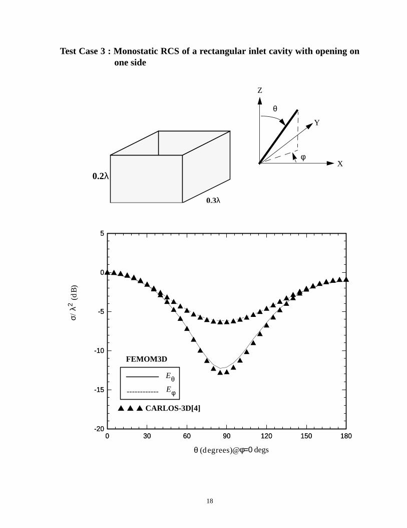
Test Case 3 : Monostatic RCS of a rectangular inlet cavity with opening onone side

0.2λ

0.3λ0.3λ

X

Z

Y

θ

φ

0 30 60 90 120 150 180-20

-15

-10

-5

0

5

0 30 60 90 120 150 180-20

-15

-10

-5

0

5

σ/λ2

(dB

)

------------

▲ ▲ ▲ CARLOS-3D[4]

FEMOM3D

EθEφ

θ (degrees)@ φ=0 degs

19

6.0 CONCLUDING REMARKS

The usage of FEMOM3DS code is demonstrated so that the user can get acquainted

with the details of using the code with minimum possible effort. As no software can be bug

free, FEMOM3DS is expected to have hidden bugs which can only be detected by the

repeated use of the code for a variety of geometries. Any comments or bug reports should be

sent to the authors. As the reported bugs are fixed and more features added to the code, future

versions will be released. Information on future versions of the code can be obtained from

Electromagnetics Research Branch (MS 490)Flight Electronics and Technology DivisionNASA-Langley Research CenterHAMPTON VA 23681

ACKNOWLEDGEMENTS

The authors would like to thank Mr. Fred B. Beck and Dr. C.R. Cockrell of NASA

Langley Research Center for the useful discussions and constant support during the

development of this code.

20

Appendix 1

Theory for FEMOM3DS

This appendix is intended to give a brief description of the theory behind the code.

The geometry of the structure to be analyzed is shown in figure 1. represents the outer

surface of the 3D object, represents the area of the fictitious outer boundary to be used for

terminating the FEM computational domain. The electric field inside the compuational

domain satisfies the vector wave equation[5]

(1)

where and are the relative permittivity and relative permeability of the medium. The

time dependency of is assumed through out this report. To facilitate the suitable

solution of the partial differential equation in (1) via FEM, multiply equation (1) with a vector

testing function and integrate over the volume of the computational domain. By applying

suitable vector identities, equation(1) can be written in its weak form as,

(2)

Applying the divergence theorem to the right hand side of equation(2), the volume integral is

written as the surface integral over the surface terminating the FEM computational

domain.

(3)

where is the unit outward normal to the surface .

To discretize the above volume and surface integrals, the FEM computational domain

is subdivided into small volume tetrahedral elements. The electric field is expressed in terms

of vector edge basis functions[2] which enforce the divergenceless condition of the electric

field implicitly

(4)

Sb

So

1µr----- E∇×

ko2εrE–∇× 0=

εr µr

jωt( )exp

T

1µr----- T∇×( ) 1

µr----- E∇×

dv•V∫∫∫ ko

2– εr T Edv•

V∫∫∫ T

1µr----- E∇××

dv∇•V∫∫∫=

So

1µr----- T∇×( ) E∇×( ) dv•

V∫∫∫ ko

2– εr T Edv•

V∫∫∫ T n

1µr----- E∇××

• sdSo

∫∫–=

n So

E eiW ii 1=

6

∑=

21

where ’s are the unknown coefficients associated with each edge of the tetrahedral element

and ’s are the basis functions and are given in detail in [6]. The testing function is taken

to be the same set of basis functions as given in equation (4), i.e.,

j=1,2,3,4,5,6 (5)

The discretization of the FEM computational volume automatically results in

discretization of surface in triangular elements. The evaluation of the surface integrals

over the outer boundary is evaluated either by using Method of Moments(MoM) or Absorbing

Boundary Conditions (ABCs).

Evaluation of surface integral over So - MoM formulation :

At the fictitious outer boundary the electric field is subjected to the condition that the

fields are continuous across the boundary, i.e.,

(6)

where denotes the outer side of and denotes the inner side of . The electric field

is the field quantity being evaluated in the computational volume through FEM. The

electric field ouside is evaluated explicitly using the following equation[5, eq.3-83]:

(7)

where

= Magnetic Vector Potential = (8)

ei

W i T

T W j=

So

Eat So

+ Eat So

-=

So+

So So-

So

Eat So

-

So

Eat So

+ F∇×– jωµoA–1

jωµo------------∇∇ A• Einc+ +=

A1

4π------

J jko r r o––( )exp

r r o–----------------------------------------------- sd

So

∫∫

22

= Electric Vector Potential = (9)

and

= Incident Electric Field=

where

(10)and

(11)

(12)

(13)

(14)

(15)

(16)

and are assumed to be equivalent electric and magnetic currents respectively at the outer

surface . and indicate the direction of the incident field. The terms with the magnetic

vector potential contribute to the electric field outside V due to the equivalent electric current

radiating into free space. Similarly the term with electric vector potential contribute to the

electric field outside V due to the equivalent magnetic current radiating into free space(figure

5).

Substituting equation (7) into equation (6) and multiplying by a testing function

on both sides and integrate over the surface , results in:

(17)

After some mathematical manipulations[7, pp.42], [8, pp.135], and substituting equations (8)

and (9) in the above equation, it can be rewritten as:

F1

4π------

M jko r r o––( )exp

r r o–-------------------------------------------------- sd

So

∫∫

Einc Ei j kxx kyy kzz+ +( )[ ]exp

Ei xExi yEyi zEzi+ +=

Exi θi φi αcoscoscos φi αsinsin–=

Eyi θi φi αcossincos φicos αsin+=

Ezi θi αcossin–=

kx k θi φicossin=

ky k θi φisinsin=

kz k θicos=

J M

So θi φi

n T×

So

n T×( ) E• sdSo

∫∫ n T×( ) F∇×( )• sdSo

∫∫– jωµo n T×( ) A• sdSo

∫∫–=

+1

jωεo----------- n T×( ) ∇ A•∇( )• sd

So

∫∫ n T×( ) Einc• sdSo

∫∫+

23

Figure 5 Equivalent current representation of the outer surfaceSo

J

M

SoFictitious outer boundary

n

24

(18)

where indicates that the singular point has been removed and

(19)

Equation (18) is written in a matrix form by choosing the proper basis functions for and

and accordingly using the testing function . Within each surface triangle, the surface

currents can be expressed as

(20)

(21)

and the testing function as

j=1,2,3 (22)

In equation (20), represents the same unknown coefficient as in equation (4) and in

equation(21) represents the unknown coefficient for the surface electric current densisty. In

equations (20) and (21), it is interesting to note that, the vector edge basis functions ,

which are initially used for electric field are used to represent the surface current densities in

the form of . The expansion functions are used to build tangential continuity into

the field representation. In contrast, the cross product of with these functions results in

another set of basis functions which guarantee normal continuity with zero curl and nonzero

divergence and hence are ideally suited for representing surface current densities[2]. During

12--- n T×( ) E• sd

So

∫∫ 14π------ n T×( ) M ∇'G× s'd

So

∫∫ • sd

So

∫∫+

+jωµo

4π------------ n T×( ) JG s'd

So

∫∫ • sd

So

∫∫ 1jωεo 4π( )------------------------- n T×( )∇•{ } J∇•( ) G s'd

So

∫∫{ } sdSo

∫∫+

= n T×( ) Einc• sdSo

∫∫

∫∫

Gjko r r o––( )exp

r r o–--------------------------------------------=

M J

n T×

M E n× ei n W i×( )i 1=

3

∑–= =

J I i n W i×( )i 1=

3

∑=

n T× n W j×=

ei

I i

W i

n W i× W i

n

25

the current investigation, it has been observed that the roof top basis functions for triangular

pathes used by Rao[7] and the basis functions used here proved to be numerically identical to

each other confirming the above point of view.

Equations (20-22) are substituted in equation (18) and integrated over all the triangular

patch elements on surface to obtain the following matrix equation:

(23)where

(24)

(25)

and

(26)

The singularities in evaluating the integrals in equation (25) are handled analytically by using

the closed form expressions given in[9].

Using Maxwell’s equation , the surface integral on the right hand

side of the equation (3) can be written as

(27)

By equivalence principle, it can be noted that on the surface . Substituting this

into equation (27), equation (3) can be rewritten as:

(28)

Substituting equations (4),(5) and (14) in the above equation and integrating over all the

tetrahedral elements to evaluate the volume integrals on the left hand side and integrating over

all the surface triangular elements to evaluate the surface integral on the right hand side, it can

So

M1e{ } M2

I{ }+ b1{ }=

M112--- n T×( ) E• sd

So

∫∫ 14π------ n T×( ) M ∇'G× s'd

So

∫∫ • sd

So

∫∫+=

M2

jωµo

4π------------ n T×( ) JG s'd

So

∫∫ • sd

So

∫∫ 1jωεo 4π( )------------------------- n T×( )∇•{ } J∇•( ) G s'd

So

∫∫

sdSo

∫∫+=

b1{ } n T×( ) Einc• sdSo

∫∫=

E∇× jωµoµrH–=

T n1µr----- E∇××

• sdSo

∫∫– T n H×( )• sdSo

∫∫=

J n H×= So

1µr----- T∇×( ) E∇×( ) dv•

V∫∫∫ ko

2– εr T Edv•

V∫∫∫ T J• sd

So

∫∫=

26

be written in a matrix form as

(29)

where

(30)

(31)

and {0} is the null vector. The evaluation of the volume integrals over a tetrahedral element is

given in detail in [6].

Equations (23) and (29) are combined to form a system matrix equation:

(32)

In the above system matrix and are sparse matrices and and are dense matrices

and also the total matrix is complex and non-symmetric in nature. This matrix equation is

solved using a diagonally preconditioned biconjugate gradient algorithm, where it is

necessary to store only the non zero entries of the matrix.

The solution of equation (32), enables the computation of the electric field in

the computational volume and the equivalent magentic and electric current densities on the

surface terminating the computational domain. Using the equivalent electric and magnetic

current densities on the surface terminating the computational domain, the scattered electric

far field is computed as [5]

+ (33)

where are the spherical coordinates of the observation point. The radar cross section

is given by

(34)

F1e{ } F2

I{ }+ 0{ }=

F11µr----- T∇×( ) E∇×( ) dv•

V∫∫∫ ko

2– εr T Edv•

V∫∫∫=

F2T J• sd

So

∫∫=

F1 F2

M1 M2

e

I

0

b1

=

F1 F2 M1 M2

Efscat r( )r ∞→

jkoηo

jkor–( )exp

4πr----------------------------- θθ φφ+( ) J• x′ y′,( ) jko θ x′ φcos ′y φsin+( ) z′ θcos+( )sin( )exp xd ′ y′d∫∫–=

j ko

jkor–( )exp

4πr----------------------------- θ– φ φθ+( ) M• x′ y′,( ) jko θ x′ φcos ′y φsin+( ) z′ θcos+( )sin( )exp xd ′ y′d∫∫

r θ φ, ,( )

σ 4πr2

r ∞→lim

Efscat r( ) 2

Einc r( ) 2-----------------------------=

27

Appendix 2

Listing of the Distribution Disk

/FEMOM3DS-1.0

total 32drwxr-xr-x 2 cjr 512 Jul 29 14:52 Example1/drwxr-xr-x 2 cjr 512 Jul 29 14:51 Example2/drwxr-xr-x 2 cjr 1024 Jul 29 14:52 FEMOM3DS/drwxr-xr-x 2 cjr 1024 Jul 29 14:51 PRE_FEMOM3DS/

/FEMOM3DS-1.0/PRE_FEMOM3DS

total 528-rw-r--r-- 1 cjr 6712 Jul 29 14:46 cosmos2fem.f-rw-r--r-- 1 cjr 5358 Jul 28 14:30 edge.f-rw-r--r-- 1 cjr 624 Jun 10 15:47 makefile-rw-r--r-- 1 cjr 1651 Jul 28 14:27 meshin.f-rw-r--r-- 1 cjr 1715 Jun 10 14:41 param0-rw-r--r-- 1 cjr 800 Nov 15 1994 pmax.f-rwxr-xr-x 1 cjr 472284 Jul 28 14:30 pre_femom3ds*-rw-r--r-- 1 cjr 7719 Jun 10 16:25 pre_femom3ds.f-rw-r--r-- 1 cjr 2798 Jun 10 15:46 surfel.f

/FEMOM3DS-1.0/FEMOM3DS

total 752-rw-r--r-- 1 cjr 5151 Jul 23 14:39 analy.f-rw-r--r-- 1 cjr 4583 Jul 23 14:39 basis.f-rw-r--r-- 1 cjr 4220 Jul 28 15:53 bicgdns.f-rw-r--r-- 1 cjr 2186 Jul 23 14:42 elembd.f-rw-r--r-- 1 cjr 3616 Jul 23 14:43 elmatr.f-rw-r--r-- 1 cjr 3026 Jul 23 14:44 excit.f-rwxr-xr-x 1 cjr 529008 Jul 28 15:53 femom3ds*-rw-r--r-- 1 cjr 17609 Jul 28 15:25 femom3ds.f-rw-r--r-- 1 cjr 3028 Jul 23 14:44 fourierxy.f-rw-r--r-- 1 cjr 801 Jul 23 15:33 makefile-rw-r--r-- 1 cjr 1738 Jul 28 14:38 param-rw-r--r-- 1 cjr 1269 Jul 23 14:47 pleq.f-rw-r--r-- 1 cjr 5321 Jul 23 14:48 quadpts.f-rw-r--r-- 1 cjr 3410 Jul 23 14:48 scatter.f-rw-r--r-- 1 cjr 307 Nov 17 1994 second.f-rw-r--r-- 1 cjr 1826 Jul 23 14:48 triangeh.f

28

-rw-r--r-- 1 cjr 3137 Jul 23 14:49 triangej.f-rw-r--r-- 1 cjr 3321 Jul 23 14:49 triangej0.f-rw-r--r-- 1 cjr 2681 Jul 23 14:50 triangej01.f-rw-r--r-- 1 cjr 3494 Jul 23 14:51 triangem.f-rw-r--r-- 1 cjr 2082 Jul 23 14:51 triangem0.f-rw-r--r-- 1 cjr 1572 Jul 23 14:51 unorm.f-rw-r--r-- 1 cjr 856 Jul 23 14:53 vcross.f-rw-r--r-- 1 cjr 768 Jul 23 14:53 vdot.f-rw-r--r-- 1 cjr 5028 Jul 23 14:54 zmatrixeh.f-rw-r--r-- 1 cjr 8817 Jul 23 15:46 zmatrixej.f-rw-r--r-- 1 cjr 7591 Jul 23 15:46 zmatrixem.f

/FEMOM3DS-1.0/Example1

total 192-rw-r--r-- 1 cjr 40 Jul 24 09:34 input-rw-r--r-- 1 cjr 22 Jul 23 15:05 sp.MAT-rw-r--r-- 1 cjr 10590 Jul 29 11:01 sp.MOD-rw-r--r-- 1 cjr 2051 Jul 29 11:04 sp.OUT-rw-r--r-- 1 cjr 19698 Jul 29 11:02 sp.PIN-rw-r--r-- 1 cjr 561 Jul 29 11:02 sp.POUT-rw-r--r-- 1 cjr 472 Jul 29 11:01 sp.SES-rw-r--r-- 1 cjr 80 Jul 29 11:04 sp_bicgd.DAT-rw-r--r-- 1 cjr 41054 Jul 29 11:02 sp_edges.DAT-rw-r--r-- 1 cjr 10873 Jul 29 11:02 sp_nodal.DAT-rw-r--r-- 1 cjr 38262 Jul 29 11:02 sp_surfed.DAT

/FEMOM3DS-1.0/Example2

total 264-rw-r--r-- 1 cjr 22 Jul 24 09:08 inlet.MAT-rw-r--r-- 1 cjr 20748 Jul 28 14:32 inlet.MOD-rw-r--r-- 1 cjr 2229 Jul 28 16:59 inlet.OUT-rw-r--r-- 1 cjr 38377 Jul 29 08:20 inlet.PIN-rw-r--r-- 1 cjr 561 Jul 29 08:20 inlet.POUT-rw-r--r-- 1 cjr 551 Jul 28 14:33 inlet.SES-rw-r--r-- 1 cjr 1520 Jul 28 16:59 inlet_bicgd.DAT-rw-r--r-- 1 cjr 74008 Jul 29 08:20 inlet_edges.DAT-rw-r--r-- 1 cjr 22352 Jul 29 08:20 inlet_nodal.DAT-rw-r--r-- 1 cjr 49110 Jul 29 08:20 inlet_surfed.DAT-rw-r--r-- 1 cjr 28 Jul 28 14:34 input

29

Appendix 3

Sample *.SES files of COSMOS/M

The geometry modelling and meshing can be accomplished by using COSMOS/M.

A variety of commands are available to define geometries. The constructed geometry is

meshed and the mesh data can be written to a file with theModinput command. Dielectric

materials are identified by using material property command before meshing the

corresponding part of the dielectric material. These are used as indices to tetrahedral elements,

which will correspond to an entry in theproblem .MAT file. Specification of the surfaces

which are perfectly conducting, surfaces forming the radiating aperture and the input plane is

accomplished by enforcing pressure boundary conditions on respective surfaces. Before the

pressure condition is specified, a load condition has to be defined to indicate what type of

surface is being specified. Load conditions of 1, 2, and 3 corresponds to perfectly conducting

surface, surface with equivalent electric current and surface with equivalent magnetic current,

respectively.

The *.SES files for the sample runs presented in section 4 are given below.

Example 1:

C*C* COSMOS/M Geostar V1.75C* Problem : sp Date : 7-29-97 Time : 8:32:50C*PT 1 0.000000 0.000000 0.000000PT 2 0.000000 0.000000 0.16PT 3 0.16 0.000000 0.000000CRCIRLE 1 1 2 3 0.160 90 1CRCIRLE 2 1 2 4 0.160 90 1SFSWEEP 1 2 1 X 360.000000 4PH 1 SF 1 0.1 0.001000 1SCALE 0.000000PART 1 1 1CLS 1PARTPLOT 1 1 1MA_PART 1 1 1 1 0 4ACTSET LC 1ACTSET LC 2

30

PSF 1 2 8 1 2 2 4ACTSET LC 3PSF 1 3 8 1 3 3 4

Example 2:

C*C* COSMOS/M Geostar V1.75C* Problem : inlet Date : 7-24-97 Time : 9:39: 5C*SF4CORD 1 -0.15 -0.15 -0.1 0.15 -0.15 -0.1 0.15 0.15 -0.1 -0.150.15 &-0.1PLANE Z 0 1VIEW 0 0 1 0SCALE 0VLEXTR 1 1 1 Z 0.2PLANE Z 0 1VIEW 1 1 1 0SCALE 0PH 1 SF 1 0.08 0.0001 1PART 1 1 1MA_PART 1 1 1 1 0 4NMERGE 1 101 1 0.0001 0 0 0NCOMPRESS 1 101CLS 1CLS 1CLS 1ACTSET LC 1PSF 1 1 1 1 1 1 4PSF 3 1 6 1 1 1 4ACTSET LC 2PSF 1 2 6 1 2 2 4ACTSET LC 3PSF 2 3 2 1 3 3 4

31

Appendix 4

Generic Input file format for PRE_FEMOM3DS

The following is the format of the generic input file (problem .PIN ) to be supplied to

PRE_FEMOM3DS with required nodal data.

Nn

Ne

Np

Na1

Na2

Ng

x1 y1 z1, ,

x2 y2 z2, ,

xNpyNp

zNp, ,

n11 n21 n31 n41, , , mg 1( )

n12 n22 n32 n42, , , mg 2( )

n1Nen2Ne

n3Nen4Ne

, , , mg Ne( )

.

.

.

.

.

● Nn: Number of nodes

● Ne : Number of trahedral elements

● Number of triangular elements onNa1 :

● Number of triangular elements on

● Maximum number of material groupsNg :

Na2 :

surfaces

surface with equivalent electric current

surface with equivalent magnetic current

● Number of triangular elemets on PECNp :

Coordinates of the nodes 1,2,3...,Nn

Node numbers connecting each tetrahedralelement1 2 3 .....,Ne, , , , and material groupindex number for each element

,

,

,

32

Ne1 n11 n21 n31, ,

Ne2 n12 n22 n32, ,

NeNpn1Np

n2Npn3Np

, ,

Ne1 n11 n21 n31, ,

Ne2 n12 n22 n32, ,

NeNa1

n1Na1n2Na1

n3Na1, ,

Ne1

Ne2 n12 n22 n32, ,

n11 n21 n31, ,

NeNa2n1Na2

n2Na2n3Na2

, ,

Global number of the terahedral element with atriangular face on PEC surface

Ne1 Ne2 ........ NeNp, , ,( )

and three nodes connecting the triangular element

Global number of the terahedral element with atriangular face on the electric current surface

Ne1 Ne2 ........ NeNa1, , ,( )

and three nodes connecting the triangular element

Global number of the terahedral element with atriangular face on the magnetic current surface

Ne1 Ne2 ........ NeNa2, , ,( )

and three nodes connecting the triangular element

,

,

,

,

,

.

.

.

.

.

.

.

,

,

,

,

.

.

.

.

.

33

REFERENCES

[1] X.Yuan, “Three dimensional electromagnetic scattering from inhomogeneous objects by

the hybrid moment and finite element method,” IEEE Trans. Mocrowave Theory and

Techniques, Vol.MTT-38, pp.1053-1058, August 1990.

[2] J.M.Jin,The Finite Element Method in Electromagnetics, John Wiley & Sons, Inc., New

York, 1993.

[3] COSMOS/M User Guide,Version 1.75, Structural Research and Analysis Corporation,

Santa Monica CA, 1996

[4] J.M.Putnam, L.N.Medgyesi-Mitchang and M.B.Gedera, “CARLOS-3D; Three

dimensional method of moments code,”McDonnell Douglas Aerospace Report, Vol. 1

& 2, 1992.

[5] R.F.Harrington,Time Harmonic Electromagnetic Fields, McGraw Hill Inc, 1961.

[6] C.J.Reddy, M.D.Deshpande, C.R.Cockrell and F.B.Beck, “Finite element method for

eigenvalue problems in electromagnetics,”NASA Technical Paper-3485,December

1994.

[7] S.M.Rao, “Electromagnetic scattering and radiation of arbitrarily shaped surfaces by

triangular patch modelling,” Ph.D. Thesis, The University of Mississippi, August 1980.

[8] R.E.Collins, Field theory of guided waves, Second Edition, IEEE Press, New York,

1991.

[9] D.R.Wilton, S.M.Rao, D.H.Shaubert, O.M. Al-Bunduck and C.M.Butler, “Potential

integrals for uniform and linear source distributions on polygonal and polyhedral

domains,”IEEE Trans. on Antennas and Propagation, Vol.AP-32, pp.276-281, March

1984.

Form ApprovedOMB No. 0704-0188

Public reporting burden for this collection of information is estimated to average 1 hour per response, including the time for reviewing instructions, searching existing data sources, gathering and maintaining the data needed, and completing and reviewing the collection of information. Send comments regarding this burden estimate or any other aspect of this collection of information, including suggestions for reducing this burden, to Washington Headquarters Services, Directorate for Information Operations and Reports, 1215 Jefferson Davis Highway, Suite 1204, Arlington, VA 22202-4302, and to the Office of Management and Budget, Paperwork Reduction Project (0704-0188), Washington, DC 20503.

1. AGENCY USE ONLY (Leave blank) 2. REPORT DATE 3. REPORT TYPE AND DATES COVERED

4. TITLE AND SUBTITLE

6. AUTHOR(S)

5. FUNDING NUMBERS

7. PERFORMING ORGANIZATION NAME(S) AND ADDRESS(ES) 8. PERFORMING ORGANIZATION REPORT NUMBER

9. SPONSORING / MONITORING AGENCY NAME(S) AND ADDRESS(ES) 10. SPONSORING / MONITORING AGENCY REPORT NUMBER

11. SUPPLEMENTARY NOTES

12a. DISTRIBUTION / AVAILABILITY STATEMENT 12b. DISTRIBUTION CODE

13. ABSTRACT (Maximum 200 words)

14. SUBJECT TERMS 15. NUMBER OF PAGES

16. PRICE CODE

17. SECURITY CLASSIFICATION OF REPORT

18. SECURITY CLASSIFICATION OF THIS PAGE

19. SECURITY CLASSIFICATION OF ABSTRACT

20. LIMITATION OF ABSTRACT

NSN 7540-01-280-5500Prescribed by ANSI Std. Z39-18298-102

Standard Form 298 (Rev. 2-89)

REPORT DOCUMENTATION PAGE

August 1997 Contractor Report

User's Manual for FEMOM3D3, Version 1.0 NCC1-231

WU 522-33-11

C. J. ReddyM. D. Deshpande

Hampton UniversityHampton, VA 23368

National Aeronautics and Space AdministrationLangley Research CenterHampton, VA 23681-0001

NASA CR-201730

Langley Technical Monitor: Fred B. Beck

Unclassified - UnlimitedSubject Category 32

FEMOM3DS is a computer code written in FORTRAN 77 to compute electromagnetic(EM) scattering characteristics of a three dimensional object with complex materials using combined Finite Element Method(FEM)/Method of Moments (MoM) technique. This code uses the tetrahedral elements, with vector edge basis functions for FEM in the volume of the cavity and the triangular elements with the basis functions similar tothat described for MoM at the outer boundary. By virtue of FEM, this code can handle any arbitrarily shaped three-dimensional cavities filled with inhomogeneous lossy materials. The User's Manual is writtento make the user acquainted with the operation of the code. The user is assumed to be familiar with the FORTRAN 77 language and the operating environment of the computers on which the code is intended to run.

Electromagnetic scattering, cavities, Finite Element Method, Method of Moments, Hybrid Methods

35

A03

Unclassified Unclassified