User's Manual for FEMOM3DR - NASA w/g or I \ Cir w/g) / \ / J Fictitious outer boundary So Figure 1...

$: User's Manual for FEMOM3DR - NASA w/g or I \ Cir w/g) / \ / J Fictitious outer boundary So Figure 1 Illustration of cavity-backed radiating aperture in a 3D PEC body. The cavity is$
NASA / CR- 1998-208709

User's Manual for FEMOM3DR

Version 1.0

C. J. Reddy

Hampton University, Hampton, Virginia

National Aeronautics andSpace Administration

Langley Research CenterHampton, Virginia 23681-2199

Prepared for Langley Research Centerunder Cooperative Agreement NCC 1-231

September 1998

https://ntrs.nasa.gov/search.jsp?R=19980237194 2018-09-01T00:59:47+00:00Z

Available from the following:

NASA Center for AeroSpace Information (CASI)7121 Standard Drive

Hanover, MD 21076-1320

(301) 621-0390

National Technical Information Service (NTIS)

5285 Port Royal Road

Springfield, VA 22161-2171

(703) 487-4650

CONTENTS

.

2.

3.

4.

5.

Introduction

Installation of the code

Operation of the code

Sample runs

Concluding Remarks

Acknowledgements

Appendix 1

Appendix 2

Appendix 3

Appendix 4

References

Theory for FEMOM3DR

Listing of the distribution disk

Sample *.SES file of COSMOS/M

Generic input file format for PRE_FEMOM3DR

2

2

4

8

24

24

25

32

35

41

43

1. INTRODUCTION

FEMOM3DR is a computer code written in FORTRAN 77 to compute

electromagnetic(EM) radiation characteristics of antennas on a three dimensional object with

complex materials (fig. 1) using combined Finite Element Method (FEM)/Method of

Moments (MoM) technique[l]. This code uses the tetrahedral elements, with vector edge

basis functions for FEM in the volume of the cavity and the triangular elements with the basis

functions similar to that described in [2], for MoM at the outer boundary. By virtue of FEM,

this code can handle any arbitrarily shaped three-dimensional bodies filled with

inhomogeneous lossy materials. The basic theory implemented in the code is given in

Appendix 1.

The User's Manual is written to make the user acquainted with the operation of the

code. The user is assumed to be familiar with the FORTRAN 77 language and the operating

environment of the computers on which the code is intended to run. The organization of the

manual is as follows. Section 1 is the introduction. Section 2 explains the installation

requirements. The operation of the code is given in detail in Section 3. Three example runs,

the first EM radiation characteristics of an open coaxial line in a 3D PEC body, the second

radiation characteristics of an open rectangular waveguide in a 3D PEC body, and the third

EM radiation characteristics of an open circular waveguide in a three dimensional cavity are

demonstrated in Section 4. Users are encouraged to try these cases to get themselves

acquainted with the code.

2. INSTALLATION OF THE CODE

The distribution disk of FEMOM3DR is 3.5" floppy disk formatted for IBM

compatible PCs. It contains a file named feraom3dr, tar. gz. This file has to be transferred

to any UNIX machine via ftp using binary mode. On the UNIX machine, use the following

commands to get all the files.

gunzip femom3dr.tar.gz

tar -xvf femom3dr.tar

This creates a directory FEMOM3DR-I.0, which in turn contains the

2

Z

3D PEC Body

Aperture

/ I % \! \/ \

I 3D C/avity

I "r,r" \

I ,-, I

Input Plane Sin p I

\ (Coax line or I

Rect w/g or I

\ Cir w/g) /\ /

J

Fictitious outer boundary S o

Figure 1 Illustration of cavity-backed radiating aperture in a 3D PEC body.The cavity is fed by a coaxial line or a rectangular waveguide or

a circular waveguide at the input plane Sin p. The fictitious outer surfaceS O is used to terminate the FEM computational domain.

• :<.,>/<i_;i¸•;•'_._•.•i: !., ':/ <_ /

subdirectories, FEMOM3 DR (source files for the main code), PRE_FEMOM3 DR (source files

for preprocessing code), Examplel, Example2 and Example3 As the codeis written

in FORTRAN 77, with no particular computer in mind, the source code in these directories

should compile on any computer architecture without any problem. The code was successfully

complied on a SGI machine, and the compilation can be done by using a makefile file for

the different machines such as SUN, DEC or CONVEX etc. The complete listing of the

directories in the distribution disk is given in Appendix 2.

3. OPERATION OF THE CODE

The computation of EM radiation characteristics from a specific geometry with

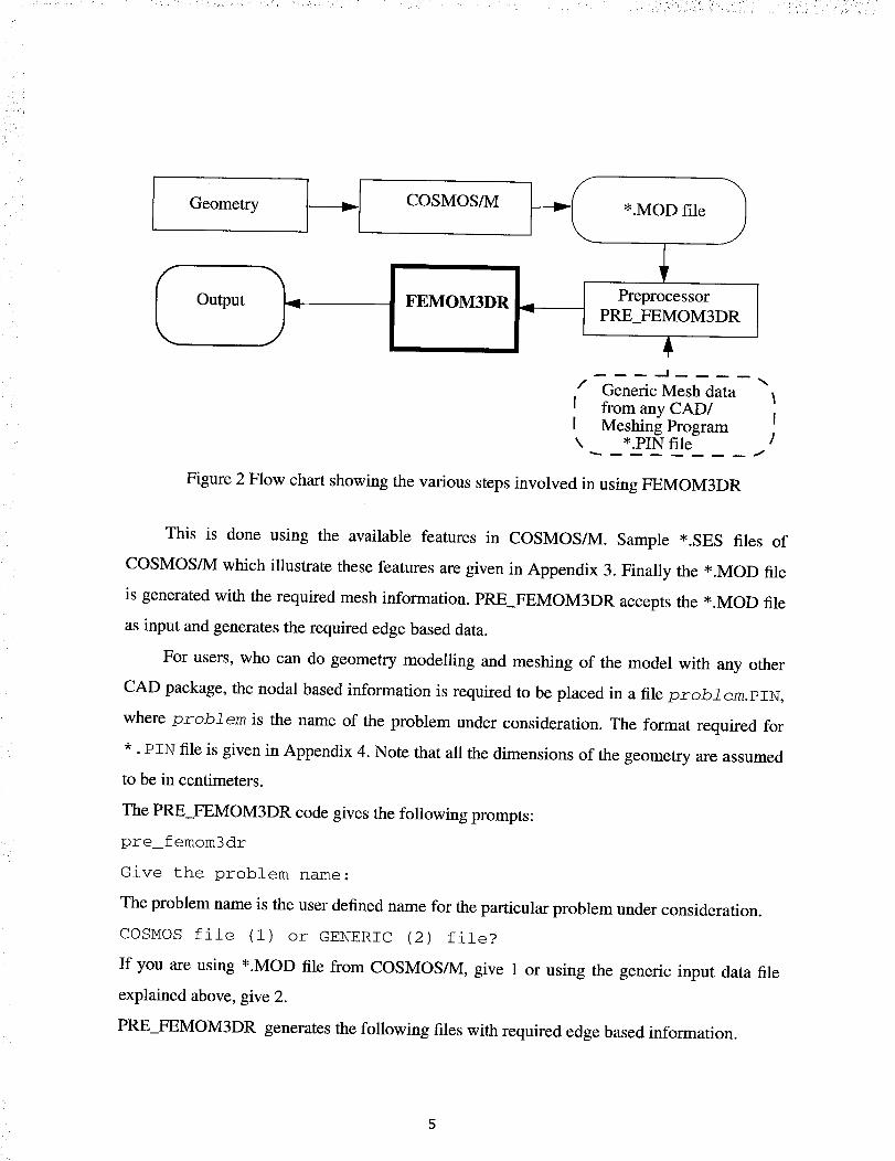
FEMOM3DR is a multi-stage process as illustrated in figure 2. The geometry of the problem

has to be constructed with the help of any commercial Computer Aided Design (CAD)

package. In our case, we used COSMOS/M[3] as our geometry modeler and meshing tool. As

FEMOM3DR uses edge based basis functions, the nodal information supplied by most of the

meshing routines cannot be readily used. Hence, a preprocessor PRE_FEMOM3DR is written

to convert the nodal based data into edge based data and then is given as input to

FEMOM3DR. For the convenience of the users, who use different CAD/meshing packages

other than COSMOS/M, PRE_FEMOM3DR accepts the nodal based data in a generic format

also. The procedures involved for using COSMOS/M input data file or generic input data file

are explained below.

With the help of COSMOS/M, the geometry is constructed and meshed with

tetrahedral elements. The user is assumed to be familiar with COSMOS/M package and its

features. Once the mesh is generated, one needs to identify the following to impose proper

boundary conditions:

(a) tetrahedral elements with different material parameters 1,

(b) elements on PEC surfaces

(c) elements on the outer boundary

(d) elements on the input plane

1. COSMOS/M has a feature by which it can group tetrahedral elements with different material proper-ties into different groups. For a generic file input, the user has to specify the material property index foreach tetrahedral element to indicate its material property group(see Appendix 4).

Oeome COSMOS ;< OD leot t). i repro esorPRE_FEMOM3DR

/ Generic Mesh data

I from any CAD/

I Meshing Program\ *.PIN file

Figure 2 Flow chart showing the various steps involved in using FEMOM3DR

)

I

/J

This is done using the available features in COSMOS/M. Sample *.SES files of

COSMOS/M which illustrate these features are given in Appendix 3. Finally the *.MOD file

is generated with the required mesh information. PRE_FEMOM3DR accepts the *.MOD file

as input and generates the required edge based data.

For users, who can do geometry modelling and meshing of the model with any other

CAD package, the nodal based information is required to be placed in a file prob2 era.PIN,

where prob2 em is the name of the problem under consideration. The format required for

*. PIN file is given in Appendix 4. Note that all the dimensions of the geometry are assumed

to be in centimeters.

The PRE_FEMOM3DR code gives the following prompts:

pre_femom3 dr

Give the problem name:

The problem name is the user defined name for the particular problem under consideration.

COSMOS file (i) or GENERIC (2) file?

If you are using *.MOD file from COSMOS/M, give 1 or using the generic input data file

explained above, give 2.

PRE_FEMOM3DR generates the following files with required edge based information.

(a) probl em_nodal. DAT - Node coordinates and the node numbers for each element

(b)prob2 era_edges. DAT - Information on edges, such as nodes connecting each edge, etc.

(c) prob2 em_s u r fed. DAT - Information on edges on outer surfaces.

(d) p r o b 1 era_ s u r f e 1. DAT - Information on edges on input surface.

(e) probl era.POUT - General information on the mesh.

The files (a) to (d) are used as input for FEMOM3DR. Users need not interact or modify the

above files.

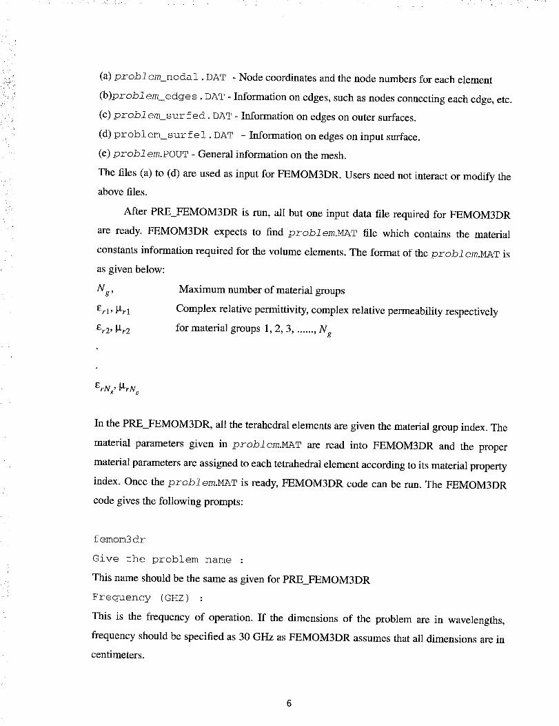
After PRE_FEMOM3DR is run, all but one input data file required for FEMOM3DR

are ready. FEMOM3DR expects to find problem.MAT file which contains the material

constants information required for the volume elements. The format of the probl em.NAT is

as given below:

Ng,

Erl, _l, rl

Er2, _l, r2

Maximum number of material groups

Complex relative permittivity, complex relative permeability respectively

for material groups 1, 2, 3, ...... , Ng

ErNg, _'LrNg

In the PRE_FEMOM3DR, all the terahedral elements are given the material group index. The

material parameters given in prob2era.NAT are read into FEMOM3DR and the proper

material parameters are assigned to each tetrahedral element according to its material property

index. Once the prob2 era.NAT is ready, FEMOM3DR code can be run. The FEMOM3DR

code gives the following prompts:

f emom3 dr

Give the problem name :

This name should be the same as given for PRE_FEMOM3DR

Frequency (GHZ) :

This is the frequency of operation. If the dimensions of the problem are in wavelengths,

frequency should be specified as 30 GHz as FEMOM3DR assumes that all dimensions are in

centimeters.

Give the type of feed line :

coax(l), rect wg(2), cir wg(3)

This is to specify the type of feed line to be used. User should give 1 if coaxial feed is used, or

2 if rectangular waveguide is used as feed, or 3 if circular waveguide is used as feed. Depending

on the feed line to be used, FEMOM3DR gives different prompts to input the feed lineparameters.

For coax(l)

Coaxial feed line

Give Inner rad, rl(cm), Outer rad, r2(cm) :

Specify the inner radius and outer radius of the coaxial line.

Dielectric const for the coaxial line, erl

Specify the dielectric constant used for the coaxial line.

Forrectwg(2)

Rectangular waveguide feed

Give waveguide dimensions :

Speci_ the waveguide dimensions,

dimension b(cm)

For cir wg(3)

Circular waveguide feed

Give the radius of circular waveguide aa(cm) :

a(cm) , b(cm)

broad wall dimension a(cm), narrow wall

Specify the radius of the circular waveguide in cms.

For computing radiation pattern, give Theta(degs) -

start angle, stop angle and increment

Specify the start and stop angles of O in degrees. Radiation patterns will be computed in both= 0 ° and ¢ = 90 ° planes.

FEMOM3DR generates the file problem.OUT, which contains information on

CPU times for matrix generation, matrix fill, the input characteristics and the radiation pattern

data. FEMOM3DR also generates another file problem bicgd.DAT which contains

information on convergence history of diagonally preconditioned biconjugate gradient

algorithm used to solve the matrix equations.

4. SAMPLE RUNS

Three example runs are illustrated in this section. They are selected to illustrate

some of the features of FEMOM3DR.

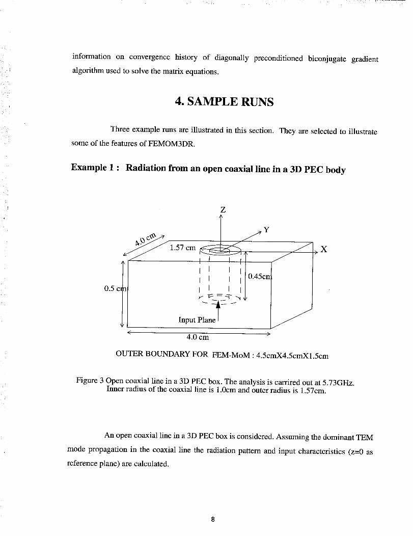
Example 1 : Radiation from an open coaxial line in a 3D PEC body

0.5 c:

Z

Y

1.57 cm

I I

i i i il

Input P_an_ _ _

< 4.0 cm >

X

OUTER BOUNDARY FOR FEM-MoM • 4.5cmX4.5cmX1.5cm

?

• i

Figure 3 Open coaxial line in a 3D PEC box. The analysis is carrired out at 5.73GHz.Inner radius of the coaxial line is 1.0cm and outer radius is 1.57cm.

An open coaxial line in a 3D PEC box is considered. Assuming the dominant TEM

mode propagation in the coaxial line the radiation pattern and input characteristics (z=0 as

reference plane) are calculated.

8

First the PRE_FEMOM3DR

cjr@caph:{53} pre_femom3dr


coax

COSMOS file(l) or GENERIC(2) file ? :

1

Opening file :coax.MOD

Read the following data

Nodes= 403

Elements= 1201

Elements on surface i=

Elements on surface 2=

Max number of material groups=

468

44

1

Forming the edges !!! Be patient !]

Order of the FEM matrix- nptrx= 1554

Number of nodes= 403

Number of elements= 1201

Number of total edges= 2001

Number of elements on Surface i=

Number of elements on Surface 2=

Number of edges on surface 0(pec)=

Number of edges on surface i=

Number of edges on surface 2=


468

44

447

702

84

1

Order of FEH matrix= 1554

Order of MoM matrix(electric cuurent)=

Unknown for the magnetic current=

Number of unknowns on Input plane=

702

48

702

Order of Hybrid FEM/MoM matrix= 2256

The coax. MAT file for this problem is given below:

i

(1.o,o.o) (1.o,o.o)

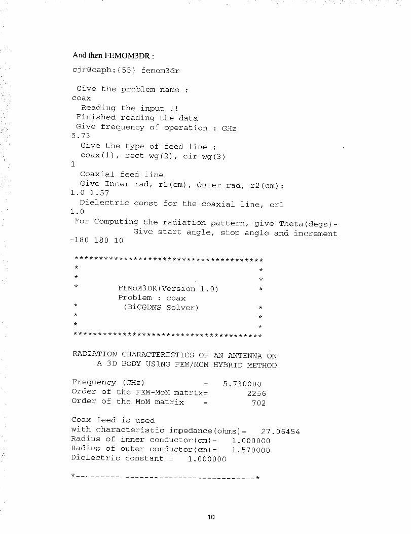
And then FEMOM3DR •

cjr@caph:{55} femom3dr


COaX

Reading the input !!

Finished reading the data

Give frequency of operation : GHz

5.73


coax(l), rect wg(2), cir wg(3

Coaxial feed line

Give Inner tad, rl(cm) , Outer rad, r2 (cm) :

1.0 1.57

Dielectric const for the coaxlal line, erl1.0

For Computing the radiation pattern, give Theta(degs)-

Give start angle, stop angle and increment-180 180 i0

* FEMoM3DR(Version 1.0) *

Problem : coax

(BiCGDNS Solver)

RADIATION CHARACTERISTICS OF AN ANTENNA ON

A 3D BODY USING FEM/MOM HYBRID METHOD

Frequency (GHz)

Order of the FEM-MoM matrix=

Order of the MoM matrix

5.730000

2256

702

Coax feed is used

with characteristic impedance(ohms)= 27.06454

Radius of inner conductor(cm)= 1.000000

Radius of outer conductor(cm)= 1.570000

Dielectric constant = 1.000000

10

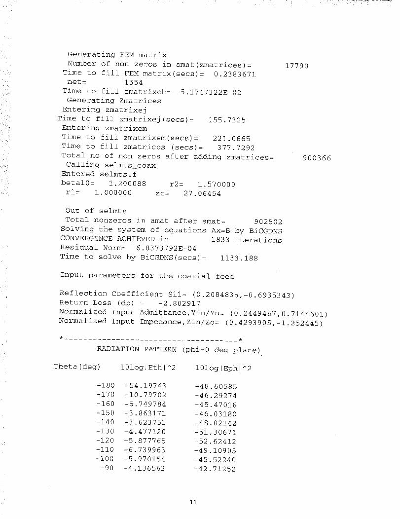
Generating FEM matrixNumber of non zeros in amat(zmatrices)=

Time to fill FEM matrix(secs)= 0.2383671net= 1554

Time to fill zmatrixeh= 5.1747322E-02Generating Zmatrices

Entering zmatrixejTime to fill zmatrixej(secs)= 155.7325

Entering zmatrixemTime to fill zmatrixem(secs)= 221.0665Time to fill zmatrices (secs)= 377.7292Total no of non zeros after adding zmatrices=

Calling selmts_coaxEntered selmts.fbetal0= 1.200088 r2= 1.570000

rl: 1.000000 zc= 27.06454

17790

900366

Out of selmtsTotal nonzeros in amat after smat= 902502

Solving the system of equations Ax:B by BiCGDNSCONVERGENCEACHIEVED in 1833 iterationsResidual Norm= 6.8373792E-04Time to solve by BiCGDNS(secs = 1133.188

Input parameters for the coaxial feed

Reflection Coefficient SII= (0.2084835,-0.6935343)Return Loss (db) = -2.802917Normalized Input Admittance,Yin/Yo= (0.2449467,0.7144601)Normalized Input Impedance,Zin/Zo= (0.4293905,-1.252445)

RADIATION PATTERN (phi=0 deg plane)

Theta(deg) 101ogJEthl^2 101ogJEphJ^2

-180-170-160-150-140-130-120-ii0-i00

-90

-54.19743-10.79702-5 749784-3 863171-3 623751-4 477120-5 877765-6 739963-5 970154-4 136563

-48 60585-46 29274-45 47018-46 03180-48 02142-51 30671-52 62412-49 10905-45 52240-42 71252

11

L; i ¸ .... i_i

-8O-70-60-50-40-30-20-i0

0i020304O5O6O708O9O

i00ii0120130140150160170180

-2.249640-0.6981635

0.40495070.97263730.8663030

-0.1586271-2.607281-8.010056-36.21795-7.811026-2.518029

-0.10835660.89743820.99437530.4234217

-0.6786989-2.226301-4.108023-5.937835-6.708505-5.847709-4.445064-3.588042-3.822448-5.698858-10.70996-54.19810

-40.37156-38.32143-36.53478-35 07118-34 02491-33 50406-33 62665-34 52869-36 36510-39 21128-42 22832-42 46354-40 67097-39 39063-38 98084-39 25732-40 00126-41 00850-42 10268-43 18414-44 28653-45 59224-47 41969-50 17274-53 34728-52 22258-48 60595

RADIATION PATTERN

Theta (deg) 101oglEthl^2

-180-170-160-150-140-130-120-ii0-i00

-90-80

-48.60547-10.82473-5 750631-3 852743-3 605450-4 451667-5 845438-6 704795-5 939765-4 112114-2 229023

(phi:90 deg plane

101ogiEphf^2

-54.19707-48 70198-46 34335-46 03323-47 45369-49 95887-50 09461-46 91512-43 87301-41.47113-39.44118

12

0I

00 _ _ _ 0 _ _ _ _ _ _ _ _ _ _ _ 0 _ _ _ _ _ _ _ _

O000011111bO 0011111111111I I I I

00000000000000000000000000

_ _ _ _ _ _ _ _ _ _ _ _ _ _ _ _ 0 _ _ _ _ _ _ _ _Illllfl dHHHHH_HH

".X

¢:

©

©

q:u©

• ,_,-,t

0

©

r._

0

_ m_ N

o M

Example 2 : Radiation from an open rectangular waveguide in a 3D PECbody

I

I0.25)_

Z

Y

J II

I I

I I

I II

.Jf

I

I I

I jr I

< > •

0.7)_

Input Plane

0.9_,

> X

OUTER BOUNDARY FOR FEM-MoM • 1.0)_X0.6)_X0.5)_

Figure 4 Open Rectangular waveguide in a 3D PEC box

An open rectangular waveguide in a 3D PEC box is considered. Assuming the

dominant TEl0 mode propagation in the waveguide the radiation pattern and input

characteristics (z=0 as reference plane) are calculated.

F_st the PRE_FEMOM3DR

c3r0eaph:{ll} pre_femom3dr


rwg

COSMOS file(l) or GENERIC(2)1

Opening file :rwg.MOD


Nodes: 565

file ? :

14

Elements: 1743

Elements on surface I= 560

Elements on surface 2= 56


Forming the edges !!! Be patient ,





Number of elements on Surface I= 560

Number of elements on Surface 2= 56

Number of edges on surface 0(pec)= 677

Number of edges on surface i= 840

Number of edges on surface 2: 95

Max number of material groups= 1

Order of FEM matrix= 2159


Unknown for the magnetic current:


84O

73

84O


cjr@caph: {12 }

The rwg. MAT file for this problem is given below:

1

(I.0,0.0) (i.0,0.0)

And _enFEMOM3DR:

cjr@caph:{18} femom3dr


rwg

Reading the input !!

Finished reading the data

Give frequency of operation : GHz

30.0


15

• •:_i_£IC_I:';_¸ _

coax(l), rect wg(2 , cir wg(3)2

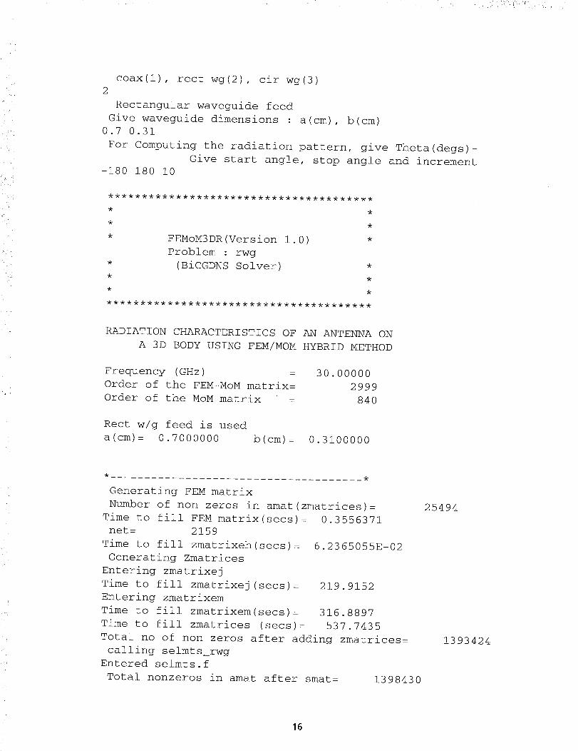
Rectangular waveguide feedGive waveguide dimensions : a(cm), b(cm)

0.7 0.31

For Computing the radiation pattern, give Theta(degs)-Give start angle, stop angle and increment

-180 180 I0

* FEMoM3DR(Version 1.0) *Problem : rwg

* (BiCGDNS Solver) *

RADIATION CHARACTERISTICSOF AN ANTENNAONA 3D BODY USING FEM/MOHHYBRID METHOD

Frequency (GHz)Order of the FEH-HoM matrix=Order of the MoM matrix

30.000002999

84O

Rect w/g feed is useda(cm)= 0.7000000 b(cm)= 0.3100000

Generating FEM matrixNumber of non zeros in amat(zmatrices)=

Time to fill FEM matrix(secs)= 0.3556371net= 2159

Time to fill zmatrixeh(secs)= 6.2365055E-02Generating Zmatrices

Entering zmatrixejTime to fill zmatrixej(secs)= 219.9152Entering zmatrixemTime to fill zmatrixem(secs)= 316.8897Time to fill zmatrices (secs)= 537.7435Total no of non zeros after adding zmatrices=

calling selmts rwgEntered selmts.f

Total nonzeros in amat after smat= 1398430

25494

1393424

16

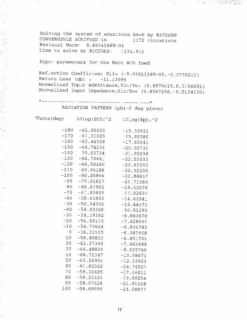
Solving the system of equations Ax=BCONVERGENCEACHIEVED in 1172Residual Norm= 8.4834168E-04Time to solve by BiCGDNS= 1134.912

by BiCGDNSiterations

Input parameters for the Rect W/G feed

Reflection CoeffReturn Loss (db)Normalized InputNormalized Input

icient SII= (-9.9301338E-05,-0.2776211= -11.13095Aclmittance,Yin/Yo= (0.8570415,0.5156051Impedance,Zin/Zo= (0.8567256,-0.5154150


Theta(deg) 101ogJEthJ^2 101ogfEphi^2

-180-170-160-150-140-130-120-ii0-i00

-90-80-70-60-50-40-30-20-i0

0i0203O4O5O607O8O90

i00

-61-61-63-68-70-66-66-69-80-75-66-61-58-56-54-54-54-54-56-58-62-66-68-65-61-59-58-58-58

.92020

.31005

.44328.7423403734704415946086186208560161767963936056189334359925061939209115736443151589853373084882071347269546234233685214310722869095

-15.32931-15.91580-17.62041-20.02731-21.95038-22 52033-22 63553-22 92205-22 88857-21 71360-19 52076-17 02657-14 62941-12 44571-i0 51392-8 882670-7 628004-6 834783-6 567938-6 851701-7 662488-8 935760-10.58671-12.53923-14.74527-17.16811-19.69254-21.91248-23.08877

17

oeol0ooo

IIIJJlll

_O_O_O__O__O_O

IIIIIIII

OOOOOOOO

HHHHHHHH

(]]

rdH

P4

O'1(1)

O

OhII

-,-'1

v

2;p4r-q

,<;

omE_

m

Cxl<

,n4J

or--IO

t_(].]

"d

rd4J¢

_ _ _ _ O _ _ O _ _ _ _ _ _ _ _ _ _ _ O _ O _ _ _ _ O _ H _ _

............ 9 H I b H b _ b H b _ H 9 ......

H H H _ _ H H H H H H H ¢ ¢ _ b b _ 9 9 b b _ _ ¢ H H H H H HIIIIIIIIIIIIIIIIIIIIIIIIiiiiiii

O O O O O O O O O O O O O O O O O O O O O O O O O O O O O O O

H H H H H H H H H I i I J I J i _ H _IIII IIII

CO

. i ":. : " _: : , ,: _. ,

130 -19.29325 -63

140 -23.87317 -61

150 -22.24701 -60

160 -18.23417 -60

170 -16.01494 -60

180 -15.32931 -61

71844

69011

44720

01572

42999

92015

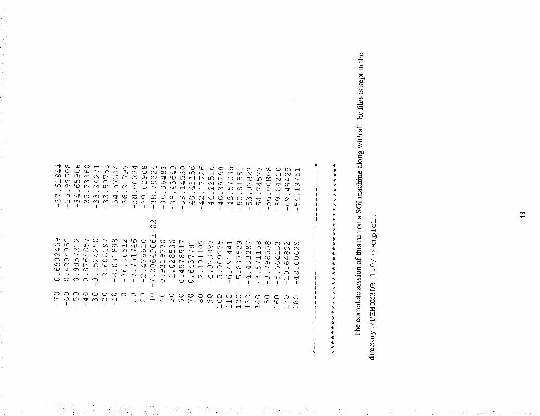
ThecompletesessionofthisrunonaSGI machinealong with all thefilesiskept

in thedirecto_ ./FEMOM3DR-I.0/Example2.

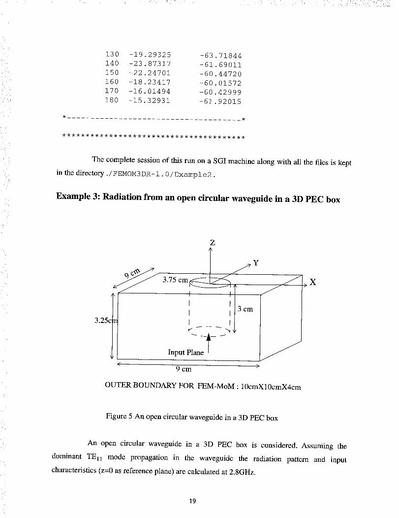
Example 3: Radiation from an open circular waveguide in a 3D PEC box

z

3.75 cm__ Y

3.251I I

I Ir_ -._

Input Plane

9 cm

OUTER BOUNDARY FOR FEM-MoM • 10cmX10cmX4cm

_>X

Figure 5 An open circular waveguide in a 3D PEC box

An open circular waveguide in a 3D PEC box is considered. Assuming the

dominant TEll mode propagation in the waveguide the radiation pattem and input

characteristics (z=0 as reference plane) are calculated at 2.8GHz.

19

Nrst_ePRE_FEMOM3DR

cjr@caph:{60} pre_femom3dr


cwg

COSMOS file(l) or GENERIC(2) file ? :

1

Opening file :cwg.MOD


Nodes= 601

Elements= 1915

Elements on surface i= 564

Elements on surface 2= 64


Forming the edges !!1 Be patient !!1





Number of elements on Surface i=

Number of elements on Surface 2=

Number of edges on surface 0(pec)=

Number of edges on surface i=

Number of edges on surface 2=


564

64

739

846

106

1

Order of FEM matrix= 2332


Unknown for the magnetic current=


846

86

846


**************************************************

The cwg. MAT fi]e_r _is problem isgiven below:

1

(i.0,0.0) (I.0,0.0)

20

cjr@caph:{65} femom3drGive the problem name :

cwgReading the input !!

Finished reading the dataGive frequency of operation : GHz

2.8Give the type of feed line :coax(l), rect wg(2), cir wg(3)

3Circular waveguide feed

Give the radius of circular waveguide aa(cm) :3.75

For Computing the radiation pattern, give Theta(degs

-180 180 I0

q

Give start angle, stop angle and increment

* FEMoM3DR(Version 1.0) *

Problem : cwg

* (BiCGDNS Solver) *

RADIATION CHARACTERISTICS OF AN ANTENNA ON

A 3D BODY USING FEM/MOM HYBRID METHOD

Frequency (GHz)

Order of the FEM-MoM matrix=

Order of the MoM matrix

2.800000

3178

846

Circular w/g feed is used

Radius of the w/g(cm): 3.750000

Generating FEM matrix

Number of non zeros in amat(zmatrices)=

Time to fill FEM matrix(secs)= 0.3919129

net= 2332

Time to fill zmatrixeh= 6.6025734E-02

Generating Zmatrices

Entering zmatrixej

27988

21

CONVERGENCEACHIEVED in 2245 iterationsResidual Norm= 8.8973634E-04Time to solve by BiCGDNS(secs)= 2174.860

Input parameters for the cir waveguide feed

Reflection Coefficient Sll= (-0.1300059,3.4798384E-02Return Loss (db) = -17.42023Normalized Input Admittance,Yin/Yo= (1.295194,-9.1804117E-02)Normalized Input Impedance,Zin/Zo= (0.7682255,5.4452278E-02)


Theta (deg) 101ogJEthi^2 101ogJEphJ^2

-180-170-160-150-140-130-120-ii0-i00

-90-80-70-60-50-40-30-20-i0

0i02O304O5O607O8090

i00ii0

-22.75692-24.54149-30.61100-27.98133-21 97158-19 15922-17 95044-17 54107-17 34824-16 88481-15 86516-14 29549-12 37232-i0 33036-8.376839-6.681361-5.375779-4.553909-4.271783-4.548341-5.365640-6.668044-8.360756-i0 30902-12 33875-14 23919-15 77886-16 77509-17 23692-17 45133

-63-60-59-58-58-59-60-61-60-58-55-53-50-48-46-45-44-44-44-44-45-47-49-51-53-55-58-61-64-64

35085635592280973494889885245042453

.0203233348213415640400042699316914799461649327148325065295658536988722321770632202592162884918311651165611861879224

22

t

Theta (deg)

120 -17

130 -19

140 -22

150 -28

160 -30

170 -24

180 -22

89702 -62

15180 -61

02265 -61

06933 -63

24335 -66

41655 -67

75692 -63

96498

55912

53593

19190

42630

00469

35098

RADIATION PATTERN

101ogJEthJ^2

-180

-170

-160

-150

-140

-130

-120

-ii0

-i00

-90

-80

-70

-60

-50

-40

-30

-20

-i0

0

i0

2O

3O

4O

50

60

7O

80

90

i00

ii0

120

-63.35092

-61.79300

-62.38220

-65.55884

-64.24979

-58.26767

-54 45654

-52 24393

-51 02455

-50 39310

-50 00290

-49 51344

-48 66899

-47 46519

-46 14532

-45 00156

-44 24279

-43 98824

-44 29570

-45 18002

-46 61389

-48 51177

-50 69865

-52 88061

-54 68048

-55 80803

-56 25292

-56 26787

-56 18223

-56 26547

-56 69032

(phi=90 deg plane)

101og[EphJ^2

-22 75693

-23 50035

-25 78485

-29 34372

-32 63723

-33 54564

-31 86797

-27 87085

-23 65279

-20 07571

-17 06390

-14 43425

-12 06949

-9.930590

-8.040731

-6.461413

-5.266761

-4.522365

-4.271783

-4.530254

-5.283057

-6.487364

-8.078716

-9.984387

-12.14472

-14.53915

-17.21146

-20.28884

-23.97681

-28.39919

-32.71435

r

23

• : _5 i ¸¸¸ -=_

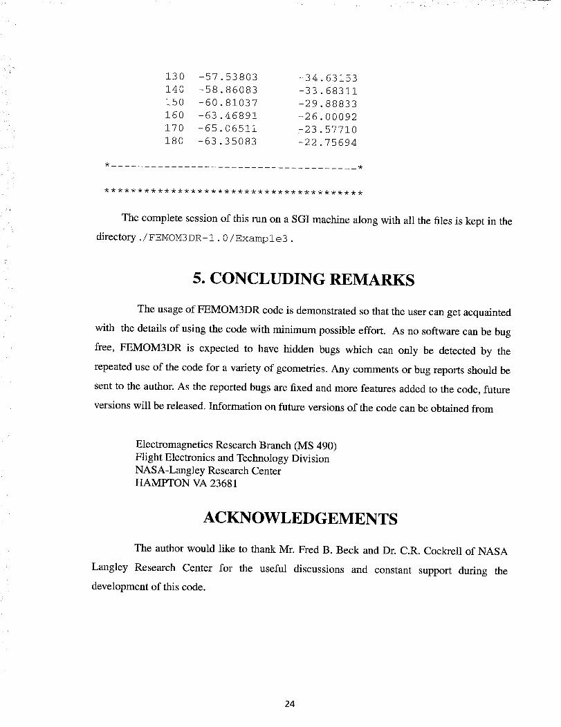
130 -57.53803 -34

140 -58.86083 -33

150 -60.81037 -29

160 -63.46891 -26

170 -65.06511 723

180 -63.35083 -22

63153

68311

88833

00092

57710

75694

The complete session of this run on a SGI machine along with all the files is kept in the

directory./FENOM3 DR- 1.0 /Exampl e3.

5. CONCLUDING REMARKS

The usage of FEMOM3DR code is demonstrated so that the user can get acquainted

with the details of using the code with minimum possible effort. As no software can be bug

free, FEMOM3DR is expected to have hidden bugs which can only be detected by the

repeated use of the code for a variety of geometries. Any comments or bug reports should be

sent to the author. As the reported bugs are fixed and more features added to the code, future

versions will be released. Information on future versions of the code can be obtained from

Electromagnetics Research Branch (MS 490)

Flight Electronics and Technology Division

NASA-Langley Research CenterHAMPTON VA 23681

ACKNOWLEDGEMENTS

The author would like to thank Mr. Fred B. Beck and Dr. C.R. Cockrell of NASA

Langley Research Center for the useful discussions and constant support during the

development of this code.

24

; _.! L

Appendix I

Theory for FEMOM3DR

This appendix is intended to give a brief description of the theory behind the code.

The geometry of the structure to be analyzed is shown in figure 1. S O represents the area of

the fictitious outer boundary to be used for terminating the FEM computational domain and

Sin p represents the area of the input plane. The electric field inside the compuational domain

satisfies the vector wave equation[4]

V× V×E -ko%E = 0 (1)

where er and [tr are the relative permittivity and relative permeability of the medium. The

time dependency of exp(j0)t) is assumed through out this report. To facilitate the suitable

solution of the partial differential equation in (1) via FEM, multiply equation (1) with a vector

testing function T and integrate over the volume of the computational domain. By applying

suitable vector identities, equation(I) can be written in its weak form as,

sssV V V

Applying the divergence theorem to the fight hand side of equation(2), the volume integral is

written as sum of the surface integral over the surface S o terminating the FEM computational

domain and the surface integral over Sin p at the input plane.

sssL<vx,,.<, =V V S o

--S S Tll//'_iX_rVXE+)ds (3)

Sinp

where h o is the unit outward normal to the surface S O and h i is the unit outward normal to the

surface Sin p .

To discretize the above volume and surface integrals, the FEM computational domain

is subdivided into small volume tetrahedral elements. The electric field is expressed in terms

25

of vector edge basis functions[2] which enforce the divergenceless condition of the electric

field implicitly

6

E = _._ eiW i (4)

i=1

where e i's are the unknown coefficients associated with each edge of the tetrahedral element

and W i's are the basis functions and are given in detail in [5]. The testing function T is taken

to be the same set of basis functions as given in equation (4), i.e.,

T = Wj j:1,2,3,4,5,6 (5)

The discretization of the FEM computational volume automatically results in

discretization of surfaces S O and Sin p in triangular elements. The evaluation of the surface

integral over the outer boundary is carried out either by using Method of Moments(MoM) and

the evaluation of the surface integral over the input plane is carried out using mode matching

method.

Evaluation of surface integral over S o - MoM formulation:

At the fictitious outer boundary the electric field is subjected to the condition that the

fields are continuous across the boundary, i.e.,

E at SO+= Elat S O (6)

+

where S O denotes the outer side of S O and S O denotes the inner side of S O. The electric field

E at s O is the field quantity being evaluated in the computational volume through FEM. The

electric field ouside S O is evaluated explicitly using the following equation[4, eq.3-83]:

where

E at So+ = -- VxF - jCogoA + J°_go"1 VV • A (7)

and

1 ffJexp(-jko[r-rol)dsA = Magnetic Vector Potential = 4-_.1 ..I _ _o]

So I I

26

(8)

:_<" i .... i_

1 ffMexp(-jko[r-r o )dsF = ElectricVectorPotential= _-_jj ]Ir_ roj[

So

(9)

J and M are assumed to be equivalent electric and magnetic currents respectively at the outer

surface S O . The equivalent currents radiating in free space are used in the equation (7) to

compute the electric field outside V (figure 6).

Substituting equation (7) into equation (6) and multiplying by a testing function

h o × T on both sides and integrate over the surface So, results in:

So S O SO

-L-f f(h+ jO)eoja_ o × T) * (VV * A)ds (10)

5'0

After some mathematical manipulations [6, pp.42], [7, pp.135], and substituting equations (8)

and (9) in the above equation, it can be rewritten as:

J°)lXoff (h°+ 47_ JJ

So

x,,,.Os,G<,s?sSo

+j_e](4rt)lS_{V*(ho xT)}{S_(V*J)Gds'}ds_ O (11)

where # indicates that the singular point has been removed and

G = exp(-jkolr - ro[)

r - ro[ (12)

Equation (11) is written in a matrix form by choosing the proper basis functions for M and J

and accordingly using the testing function h o × T. Within each surface triangle, the surface

currents can be expressed as

27

/

/

/

/

I

I

\\

f

\

I

no

t j

\\

Fictitious outer boundary S O

M

I

\

\

JJ

\\

/

\

|

II

II

Figure 6 Equivalent current representation of the outer surface S O

28

.... : _ :-i ¸::7 ' '!>:i_: ¸

M = E×h °

3

= -- 2 ei(no X Wi)

i=1

(13)

and the testing function as

J

3

_._ Ii(h o x Wi)

i=1

(14)

h o x T = h o x Wj j=1,2,3 (15)

In equation (13), e i represents the same unknown coefficient as in equation (4) and in

equation(14) I i represents the unknown coefficient for the surface electric current densisty. In

equations (13) and (14), it is interesting to note that, the vector edge basis functions Wi,

which are initially used for electric field are used to represent the surface current densities in

the form of h o x W i . The expansion functions W i are used to build tangential continuity

into the field representation. In contrast, the cross product of h o with these functions results

in another set of basis functions which guarantee normal continuity with zero curl and

nonzero divergence and hence are ideally suited for representing surface current densities[2].

During the current investigation, it has been observed that the roof top basis functions for

triangular patches used by Rao[6] and the basis functions used here proved to be numerically

identical to each other confirming the above point of view.

Equations (13-14) are substituted in equation (1 1) and integrated over all the triangular

patch elements on surface S O to obtain the following matrix equation:

whereIMll{e} + IM21{/} = {0} (16)

E ,J: S'"°x + S'"°x'<" x ) S,o

[M21 - 4re jj

So S o

(17)

+ j_¢_'(4=)S_ {V'(h°xT)}tS_ (V'J)Gds'}ds (18)

29

and {0} is the null vector.The singularitiesin evaluatingthe integralsin equation(18) are

handledanalyticallyby usingtheclosedform expressionsgivenin [8].

UsingMaxwell's equationVxE = -jO3gogrH , the surface integral on the right hand

side of the equation (3) can be written as

SoX_rVXE_s-f f T°(niXLVxE_ds : ffT'(hoXI-I)ds

Si.. \ _1,r J So

-t-f f T.(hixI-Iinp)ds (19)

Sinp

where l-Iinp is the magnetic field over the input plane obtained from matching the modal

expansion of waveguide fields with the unknowns fields at the input plane[9]. By equivalence

principle, it can be noted that J = h o x H on the surface S O. Substituting this into equation

(19), equation (3) can be rewritten as:

_r = ° °Iff (VxT)° fffT °Edv ffT Jds+ffT (hixI-Iinp)d S (20)(V×E)dv-G2

V V S O Si,,p

Substituting equations (4), (5) and I-Iinp in the above equation and integrating over all the

tetrahedral elements to evaluate the volume integrals on the left hand side and integrating over

all the surface triangular elements to evaluate the surface integrals on the right hand side, it

can be written in a matrix form as

[Fll{e}+ IF21{I} = {b 1} (21)

where [F1] includes the volume integration and the surface integration over the input place

due to mode matching,

IF:] : f f T. Jds (22)

So

and {b 1} is the excitation vector due to the dominant mode incident in the waveguide. The

evaluation of the volume integrals over a tetrahedral element is given in detail in [5].

Equations (21) and (15) are combined to form a system matrix equation:

(23)

30

_,__i_

,i,i_!ii I

In the above system matrix F 1 and F 2 are sparse matrices and M 1 and M 2 are dense matrices

and also the total matrix is complex and non-symmetric in nature. This matrix equation is

solved using a diagonally preconditioned biconjugate gradient algorithm, where it is

necessary to store only the non zero entries of the matrix.

The solution of equation (23), enables the computation of the electric field in the

computational volume and the equivalent magentic and electric current densities on the

surface terminating the computational domain. Using the equivalent electric and magnetic

current densities on the surface terminating the computational domain, the radiated electric far

field is computed as [4]

eX or)ff ^^E frad(r) r-_ _ = -Jk ° rl° ( 00 + (p_ )

• J(x', y')exp(jkosin(O(x'cos( _ + 'y sinq_) + z'cosO))dx'dy"

exp (-Jkor) ,, ....

+ Jk° 4ltr JJ(-0d_ + q_0)

• M(x', y')exp(jkosin(O(x'cos _ + 'y sind_) + z'cosO))dx'dy" (24)

where (r, 0, q_) are the spherical coordinates of the observation point. The solution of

equation (23) will also enables the calculation of electric field at the input plane, which can be

used to calculte the reflection coefficient F at the input plane [9]. The input admittance is then

calculated as

_ (l-F)Yin ( 1 + F) Yo (25)

where Yo is the characteristic admittance of the feed transmission line.

31

Appendix 2

Listing of the Distribution Disk

/FEMOM3DR-1.0

total i0

drwxr-xr-x 2 cjr 1024 Jul





2 09:47 Examplel/

2 09:48 Example2/

2 09:49 Example3/

2 09:50 FEMOM3DR/

2 09:51 PRE_FEMOM3DR/

/FEHOM3DR-I.0/PRE_FEHOM3DR

total 63

-rw-r--r--

-rw-r--r--

-rw-r--r--

-rw-r--r--

-rw-r--r--

-rw-r--r--

-rw-r--r--

-rw-r--r--

-rw-r--r--

1 cjr 202 Jul

1 cjr 6741 Oct 31

1 cjr 5295 Oct 31

1 cjr 307 Oct 31

1 cjr 1076 Oct 31

1 cjr 1723 Oct 31

1 cjr 1289 Oct 31

1 cjr

1 cjr

/FEMOM3DR-I.0/FEMOM3DR

total 380

-rw-r--r-- 1 cjr

-rw-r--r-- 1 cjr

-rw-r--r-- 1 cjr

-rw-r--r-- 1 cj r

-rw-r--r-- 1 cjr

-rw-r--r-- 1 cjr

-rw-r--r-- 1 cjr

-rw-r--r-- 1 cj r

-rw-r--r-- 1 cjr

-rw-r--r-- 1 cjr

-rw-r--r-- 1 cjr

-rw-r--r-- 1 cjr

-rw-r--r-- 1 cj r

-rw-r--r-- 1 cj r

2 09:52 README

1997 cosmos2fem.f

1997 edge.f

1997 makefile

1997 meshin.f

1997 param0

1997 pmax.f

9090 Hay 20 14:02 pre_femom3dr.f

3854 Oct 31 1997 surfel.f

472 Jul

4825 Oct 30

4195 Oct 30

885 Oct 30

984 Oct 30

i010 Oct 30

2 09.:51 README

1997 analy.f

1997 basis.f

1997 bessj.f

1997 bessj0.f

1997 bessjl.f

3921 Jun ii 09:40 bicgdns.f

2027 Oct 30 1997 elembd.f

4090 May 14 16:03 elmatr.f

21317 Jul 1 10:14 femom3dr.f

1887 Oct 30 1997 fourier_rwg.f

2640 Oct 30 1997 fourierxy.f

658 Jun 5 14:37 makefile

4405 Jul 1 09:59 param

32

-rw-r--r-- 1 cjr-rw-r--r-- 1 cjr-rw-r--r-- 1 cj r-rw-r--r-- 1 cj r-rw-r--r-- 1 cjr-rw-r--r-- 1 cjr-rw-r--r-- 1 cjr-rw-r--r-- 1 cjr-rw-r--r-- 1 cjr-rw-r--r-- 1 cjr-rw-r--r-- 1 cjr-rw-r--r-- 1 cjr-rw-r--r-- 1 cjr-rw-r--r-- 1 cjr-rw-r--r-- 1 cjr-rw-r--r-- 1 cjr-rw-r--r-- 1 cjr-rw-r--r-- 1 cjr-rw-r--r-- 1 cjr-rw-r--r-- 1 cjr-rw-r--r-- 1 cjr-rw-r--r-- 1 cjr-rw-r--r-- 1 cjr-rw-r--r-- 1 cjr-rw-r--r-- 1 cjr-rw-r--r-- 1 cjr

/FEHOM3DR-l.0/Examplel

total 1684

-rw-r--r--

-rw-r--r--

-rw-r--r--

-rw-r--r--

-rw-r--r--

-rw-r--r--

-rw-r--r--

-rw-r--r--

-rw-r--r--

-rw-r--r--

-rw-r--r--

-rw-r--r--

1 c-r

1 c-r

1 c-r

1 cDr

1 c3r

1 c3r

1 c3r

i c3r

1 c-r

1 c-'r

1 c-r

1 c-r

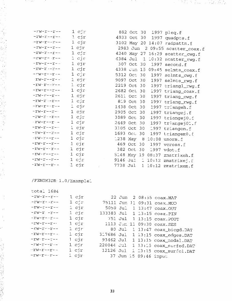
882 Oct 30 1997 pleq.f

4933 Oct 30 1997 quadpts.f

3102 May 20 14:07 radpattn.f

2983 Jun 2 09:55 scatter_coax.f

4240 May 27 16:29 scatter_cwg.f

4384 Jul 1 10:32 scatter rwq.f

307 Oct 30 1997 second.f

4338 Jun 15 09:45 selmts_coax.f

5312 Oct 30

9097 Oct 30

2219 Oct 30

2682 Oct 30

2611 Oct 30

819 Oct 30

1438 Oct 30

2905 Oct 30

3089 Oct 30

2449 Oct 30

3105 Oct 30

1693 Oct 30

1997 selmts_cwg.f

1997 selmts_rwg.f

1997 triangl_rwg.f

1997 triang_coax.f

1997 trlang_cwg.f

1997 trlang_rwg.f

1997 triangeh.f

1997 trlangej.f

1997 trlangej0.f

1997 triangej01.f

1997 triangem.f

1997 trlangem0.f

1238 May 8 10:08 unorm.f

469 Oct 30 1997 vcross.f

382 Oct 30 1997 vdot.f

5148 Hay 19 08:37 zmatrixeh.f

9146 Jul 1 10:12 zmatrixej.f

7738 Jul 1 10:12 zmatrixem.f

22 Jun 2 08:55 coax.MAT

75111 Jun ii 09:31 coax.MOD

5050 Jul 1 13:47 coax. OUT

133383 Jul 1 13:15 coax. PIN

751 Jul 1 13:15 coax. POUT

1113 Jun ii 09:30 coax. SES

80 Jul

317686 Jul

93462 Jul

220044 Jul

12126 Jul

1 13:47 coax_bicgd. DAT

1 13:15 coax_edges.DAT

1 13:15 coax_nodal.DAT

1 13:15 coax_surfed. DAT

1 13:15 coax_surfel.DAT

37 Jun 15 09:46 input

33

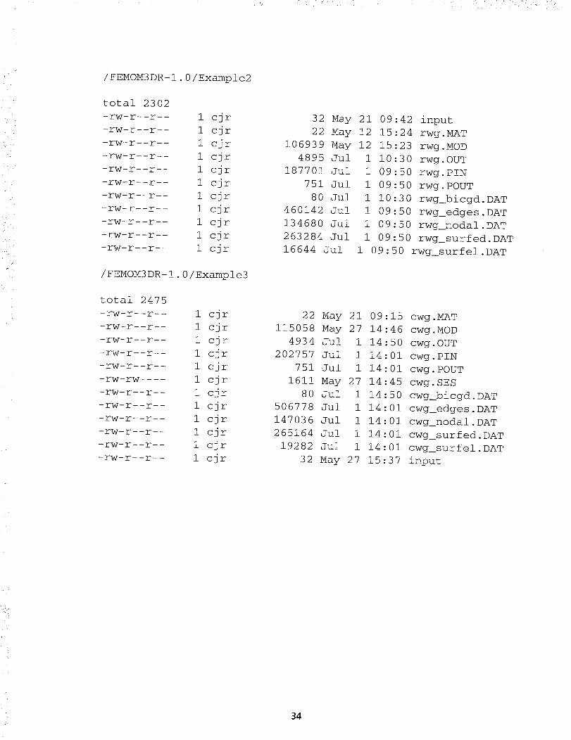
/FEMOM3DR-I.0/Example2

total 2302

-rw-r--r-- 1 c3r

-rw-r--r-- 1 cjr

-rw-r--r-- 1 cjr

-rw-r--r-- 1 cjr

-rw-r--r-- 1 cjr

-rw-r--r-- 1 cjr

-rw-r--r-- 1 cjr

-rw-r--r-- 1 cj r

-rw-r--r-- 1 cjr

-rw-r--r-- 1 cjr

-rw-r--r-- 1 cjr

/FEMOM3DR-I.0/Example3

total 2475

-rw-r--r-- 1

-rw-r--r-- 1

-rw-r--r-- 1

-rw-r--r-- 1

-rw-r--r-- 1

-rw-rw .... 1

-rw-r--r-- 1

-rw-r--r-- 1

-rw-r--r-- 1

-rw-r--r-- 1

-rw-r--r-- 1

-rw-r--r-- 1

c3r

c3r

c3r

c3r

c3r

c-r

C-r

C-r

c-r

c3r

cjr

cjr

32 Hay 21 09:42 input

22 Hay 12 15:24 rwg.HAT

106939 Hay 12 15:23 rwg.HOD

4895 Jul 1 10:30 rwg. OUT

187701 Jul 1 09:50 rwg. PIN

751 Jul 1 09:50 rwg. POUT

80 Jul 1 10:30 rwg_bicgd. DAT

460142 Jul 1 09:50 rwg_edges.DAT

134680 Jul 1 09:50 rwg_nodal.DAT

263284 Jul 1 09:50 rwg_surfed. DAT

16644 Jul 1 09:50 rwg_surfel.DAT

22 May 21 09:15 cwg.HAT

115058 May 27 14:46 cwg.MOD

4934 Jul 1 14:50 cwg. OUT

202757 Jul 1 14:01 cwg. PIN

751 Jul 1 14:01 cwg. POUT

1611 May 27 14:45 cwg. SES

80 Jul 1 14:50 cwg_bicgd. DAT

506778 Jul 1 14:01 cwg_edges.DAT

147036 Jul 1 14:01 cwg_nodal.DAT

265164 Jul 1 14:01 cwg_surfed. DAT

19282 Jul 1 14:01 cwg_surfel.DAT

32 Hay 27 15:37 input

34

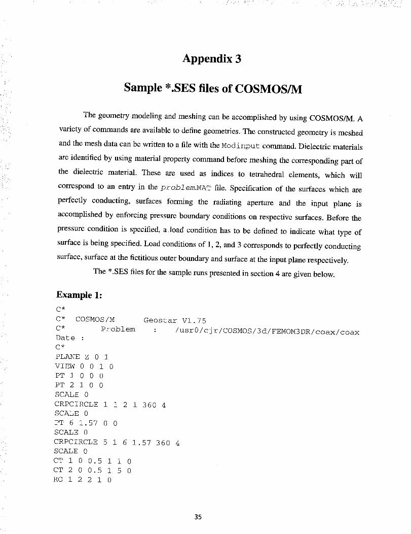
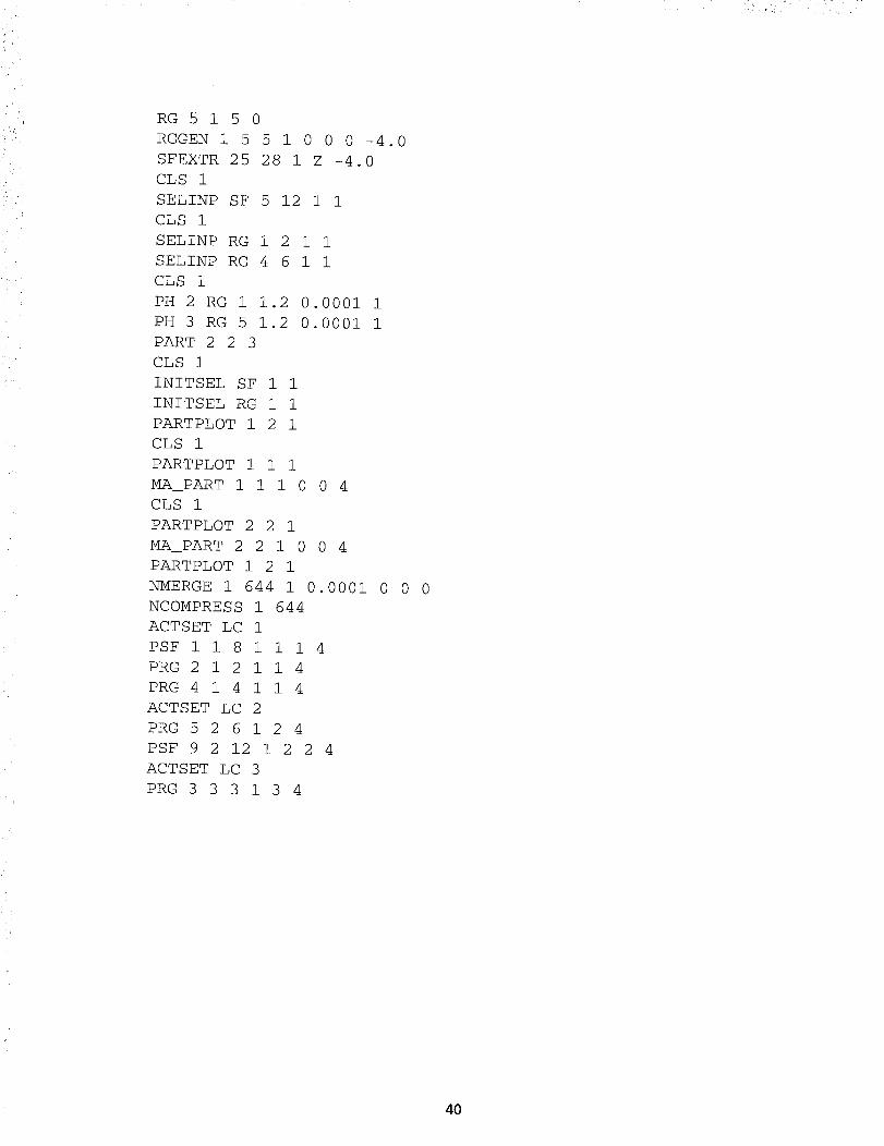
Appendix 3

Sample *.SES files of COSMOS/M

The geometry modeling and meshing can be accomplished by using COSMOS/M. A

variety of commands are available to define geometries. The constructed geometry is meshed

and the mesh data can be written to a file with the Modinput command. Dielectric materials

are identified by using material property command before meshing the corresponding part of

the dielectric material. These are used as indices to tetrahedral elements, which will

correspond to an entry in the probl em._T file. Specification of the surfaces which are

perfectly conducting, surfaces forming the radiating aperture and the input plane is

accomplished by enforcing pressure boundary conditions on respective surfaces. Before the

pressure condition is specified, a load condition has to be defined to indicate what type of

surface is being specified. Load conditions of 1, 2, and 3 corresponds to perfectly conducting

surface, surface at the fictitious outer boundary and surface at the input plane respectively.

The *.SES files for the sample runs presented in section 4 are given below.

Example 1:

C*

C* COSMOS/M

C* Problem

Date :

C*

PLANE Z 0 1

VIEW 0 0 1 0

PTI000

PT2100

SCALE 0

CRPCIRCLE 1 1 2 1 360 4

SCALE 0

PT 6 1.57 0 0

SCALE 0

CRPCIRCLE 5 1 6 1.57 360 4

SCALE 0

CT 1 0 0.5 1 1 0

CT 2 0 0.5 1 5 0

RGI2210

Geostar VI.75

: /usrO/cjr/COSMOS/3d/FEMOM3DR/coax/coax

35

1.0t_

J'_ i

iI

i

CLS 1

ACTSET LC 3

PRG 1 3 1 1 3 4

Example 2:

C*

C*

C*

7

C*

COSMOS/M Geostar VI.75

Problem : /usrO/cjr/COSMOS/3d/FEMOM3DR/rwg Date :

C* FILE rwg.in 1 1 1 1

SF4CORD 1 -0.35 -0.155 0 0.35 -0.155 0 0.35 0.155 0 -0.35 0.1550

SCALE 0

SFEXTR 1 4 1 Z -0.25

SCALE 0

CLS 1

SF4CR 6 5 12 8 ii 0

PH 1 SF 1 0.i 0.001 1

PT 9 -0.45 -0.25 0

PT i0 0.45 -0.25 0

PT ii 0.45 0.25 0

PT 12 -0.45 0.25 0

SCALE 0

CRLINE 13 9 i0

CRLINE 14 i0 ii

CRLINE 15 ii 12

CRLINE 16 12 9

CT 1 0 0.I 4 1 2 3 4 0

CT 2 0 0.i 4 13 14 15 16 b

RG 1 2 2 1 0

SFEXTR 13 16 1 Z -0.3

CLS 1

SF4CR ii 17 20 22 24 0

SF4CORD 12 -0.5 -0.3 0.i 0.5 -0.3 0.i 0.5 0.3 0.i -0.5 0.3 0.iSCALE 0

SFEXTR 25 28 1 Z -0.5

CLS 1

SF4CR 17 29 36 32 35 0

CLS 1

PHPLOT 1 1 1

SELINP SF 1 1 1 1

SELINP SF 7 ii 1 1

SELINP RG 1 1 1 1

CLS 1

37

PH 2 SF 7 0.i 0.001 i

CLS i

UNSELINP SF i i i i

UNSELINP SF 7 ii i i

UNSELINP RG 1 1 1 1

SELINP SF 12 17 1 1

PH 3 SF 12 0.i 0.001 1

PART 1 1 1

PART 2 2 3

CLS 1

PARTPLOT 2 2 1

PARTPLOT 1 2 1

MPROP 1 PERMIT 1

MA_PART 1 1 1 0 0 4

MA_PART 2 2 1 0 0 4

N-MERGE 1 605 1 0.0001 0 0 0

NCOMPRESS 1 605

CLS 1

INITSEL,SF,I,I

INITSEL,RG, I,I

CLS 1

ACTSET LC 1

PSF 2 1 5 1 1 1 4

PSF 7 1 ii 1 1 1 4

PRGIIIII4

ACTSET LC 2

PSF 12 2 17 1 2 2 4

ACTSET LC 3

PSF 6 3 6 1 3 3 4

Example 3:C*

C* COSMOS/M

C* Problem : cwg

C*

C* FILE cwg.in 1 1 1 1

PLANE Z 0 1

VIEW 0 0 1 0

PT 1 0 0 0

PT 2 3.75 0 0

CRPCIRCLE 1 1 2 3.75 360 4

SCALE 0

CT 1 0 1.2 1 1 0

RG 1 1 1 0

PT 6 -4.5 -4.5 0

PT 7 4.5 -4.5 0

Geostar VI.75

Date : 5-27-98 Time : 15: 3:49

38

/<i_ i!_ _ _, _ _ _ _ _ " L< I _ _

PT 8 4.5 4.5 0

PT 9 -4.5 4.5 0

SCALE 0

CRLINE 5 6 7

CRLINE 6 7 8

CRLINE 7 8 9

CRLINE 8 9 6

CT 2 0 1.2 1 5 0

RG22210

SFEXTR 1 4 1 Z -3.0

VIEW 1 1 1 0

RGGEN 1 1 1 1 0 0 0 -3.0

PT 14 -4.5 -4.5 -3.25

PT 15 4.5 -4.5 -3.25

PT 16 4.5 4.5 -3.25

PT 17 -4.5 4.5 -3.25

CLS 1

CLS 1

SCALE 0

SCALE 0

CRLINE 17 14 15

CRLINE 18 15 16

CRLINE 19 16 17

CRLINE 20 17 14

CT 4 0 1.2 1 20 0

RG 4 1 4 0

SFEXTR 5 8 1 Z -3.25

CLS 1

SELINP SF 1 4 1 1

SELINP RG 1 1 1 1

SELINP RG 3 3 1 1

CLS 1

PH 1 SF 1 1.2 0.0001 1

PART 1 1 1

INITSEL SF 1 1

INITSEL RG 1 1

PT 18 -5 -5 0.5

PT 19 5 -5 0.5

SCALE 0

PT20550.5

PT 21 -5 5 0.5

CRLINE 25 18 19

CRLINE 26 19 20

CRLINE 27 20 21

CRLINE 28 21 18

CT 5 0 1.2 1 28 0

39

k

RG 5 1 5 0

RGGEN 1 5 5 1 0 0 0 -4.0

SFEXTR 25 28 1 Z -4.0

CLS 1

SELINP SF 5 12 1 1

CLS 1

SELINP RG 1 2 1 1

SELINP RG 4 6 1 1

CLS 1

PH 2 RG 1 1.2 0.0001 1

PH 3 RG 5 1.2 0.0001 1

PART 2 2 3

CLS 1

INITSEL SF 1 1

INITSEL RG 1 1

PARTPLOT 1 2 1

CLS 1

PARTPLOT 1 1 1

MA_PART 1 1 1 0 0 4

CLS 1

PARTPLOT 2 2 1

MA_PART 2 2 1 0 0 4

PARTPLOT 1 2 1

NMERGE 1 644 1 0.0001 0 0 0

NCOMPRESS 1 644

ACTSET LC 1

PSF 1 1 8 1 1 1 4

PRG 2 1 2 1 1 4

PRG 4 1 4 1 1 4

ACTSET LC 2

PRG 5 2 6 1 2 4

PSF 9 2 12 1 2 2 4

ACTSET LC 3

PRG 3 3 3 1 3 4

4O

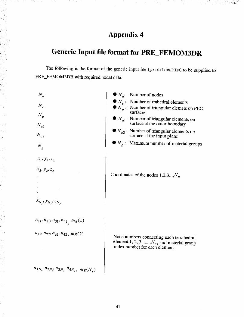
Appendix 4

Generic Input file format for PRE_FEMOM3DR

The following is the format of the generic input file (problem.PIN) to be supplied to

PRE_FEMOM3DR with required nodal data.

N n

N e

Np

Nal

Na2

N.

O Nn:ON e :

ONp:

• Nal :

• Nae :

ONe:

Number of nodes

Number of trahedral elements

Number of triangular elemets on PECsurfaces

Number of triangular elements onsurface at the outer boundary

Number of triangular elements onsurface at the input plane

Maximum number of material groups

Xl, Yl, Zl

x2, Y2, Z2

XNp' YNp' ZNp

Coordinates of the nodes 1,2,3 .... N n

nll, n21, n31, n41 mg(1)

hi2, n22, n32, n42, mg(2)

nlNe, n2N e, n3Ne, n4N_, mg(Ne)

Node numbers connecting each tetrahedral

element 1, 2, 3, ..... ,Ne, and material groupindex number for each element

41

Nel ,nll, n21, n31

Ne2 , n12, n22, n32

NeNp, nlNp, n2Np, n3Np

Nel, nll, n21, n31

Ne2, n12, n22, n32

NeN.l'nlNal' n2N_l, n3Nal

Global number of the terahedral element with atriangular face on PEC surface

( Nel' Ne2, ........ , NeNp )

and three nodes connecting the triangular element

Global number of the terahedral element with a

triangular face on the outer boudary surface

(Nel, Ne2, ........ , NeNal )


Nel , nil, n21, n31

Ne2, n12, n22, n32

NeNa2,nlNa2' n2N,,2, n3Na2

Global number of the terahedral element with a

triangular face on input plane surface

(Nel, Ne2, • ....... , NeN.2 )


42

REFERENCES

[1] X.Yuan, "Three dimensional electromagnetic scattering from inhomogeneous objects by

the hybrid moment and finite element method," IEEE Trans. Mocrowave Theory and

Techniques, Vol.MTT-38, pp. 1053-1058, August 1990.

[2] J.M.Jin, The Finite Element Method in Electromagnetics, John Wiley & Sons, Inc., New

York, 1993.

[3] COSMOS/M User Guide, Version 1.75, Structural Research and Analysis Corporation,

Santa Monica CA, 1996

[4] R.EHarrington, Time Harmonic Electromagnetic Fields, McGraw Hill Inc, 1961.

[5] C.J.Reddy, M.D.Deshpande, C.R.Cockrell and EB.Beck, "Finite element method for

eigenvalue problems in electromagnetics," NASA Technical Paper-3485, December

1994.

[6] S.M.Rao, "Electromagnetic scattering and radiation of arbitrarily shaped surfaces by

triangular patch modelling," Ph.D. Thesis, The University of Mississippi, August 1980.

[7] R.E.Collins, Field theory of guided waves, Second Edition, IEEE Press, New York,

1991.

[8] D.R.Wilton, S.M.Rao, D.H.Shaubert, O.M. A1-Bunduck and C.M.Butler, "Potential

integrals for uniform and linear source distributions on polygonal and polyhedral

domains," IEEE Trans. on Antennas and Propagation, Vol.AP-32, pp.276-281, March

1984.

[9] C.J.Reddy, M.D.Deshpande, C.R.Cockrell and EB.Beck, "Analysis of three-

dimensional-cavity-backed aperture antennas using a combined finite element method/

method of moments/geometrical theory of diffraction technique," NASA Technical

Paper 3548, November 1995.

43

REPORT DOCUMENTATION PAGE Form ApprovedOMB No. 07704-0188

Public reporting burden for this collection of information is estimated to average 1 hour per response, including the time for reviewing instructions, searching existing data source_

gathering and maintaining the data needed, and completing and reviewing the collection of information. Send comments regarding this burden estimate or any other aspect of thi

collection of information, including suggest ons for reducing this burden, to Washington Headquarters Services, Directorate for Information Operations and Reports, 1215 Jefferso

Davis Highway, Suite 1204, Arlington, VA 22202-4302 and to the Office of Management and Budget Paperwork Reduction Project (0704-0188), Washington, DC 20503.

1. AGENCY USE ONLY (Leave blank) 2. REPORT DATE 3. REPORT TYPE AND DATES COVERED

September 1998 Contractor Report

_4. TITLE AND SUBTITLE 5. FUNDING NUMBERSUser's Manual for FEMOM3DRVersion 1.0

6. AUTHOR(S)

C. J. Reddy

7. PERFORMINGORGANIZATIONNAME(S)ANDADDRESS(ES)

Hampton UniversityHampton, Virginia 23668

9. SPONSORING/MONITORING AGENCY NAME(S) AND ADDRESS(ES)

National Aeronautics and Space AdministrationNASA Langley Research CenterHampton, VA 23681-2199

11. SUPPLEMENTARY NOTES

NCC 1-231

522-11-41-02

8. PERFORMING ORGANIZATIONREPORT NUMBER

10. SPONSORING/MONITORINGAGENCY REPORT NUMBER

NASA/CR- 1998-208709

Langley Technical Monitor: Fred B. Beck

12a. DISTRIBUTION/AVAILABILITY STATEMENT

Unclassified-Unlimited

Subject Category _ _2_ Distribution: NonstandardAvailability: NASA CASI (301) 621-0390

13. ABSTRACT (Maximum 200 words)

12b. DISTRIBUTION CODE

FEMoM3DR is a computer code written in FORTRAN 77 to compute radiation characteristics of antennas on 3D

body using combined Finite Element Method (FEM)/Method of Moments (MoM) technique. The code is written to

handle different feeding structures like coaxial line, rectangular waveguide, and circular waveguide. This code uses

the tetrahedrai elements, with vector edge basis functions for FEM and triangular elements with roof-top basisfunctions for MoM. By virtue of FEM, this code can handle any arbitrary shaped three dimensional bodies with

inhomogeneous lossy materials; and due to MoM the computational domain can be terminated in any arbitraryshape. The User's Manual is written to make the user acquainted with the operation of the code. The user is

assumed to be familiar with the FORTRAN 77 language and the operating environment of the computers on whichthe code is intended to run.

14. SUBJECTTERMS

FEM, MoM, Hybrid Method, Cavity-Backed Aperture Antennas, Input Admittance,Radiation pattern

17. SECURITY CLASSIFICATIONDF REPORT

Unclassified

NSN 7540-01-280-5500

18. SECURITY CLASSIFICATIONOF THIS PAGE

Unclassified

19. SECURITY CLASSIFICATIONOF ABSTRACT

Unclassified

15. NUMBER OF PAGES

4816. PRICE CODE

A03

20. LIMITATIONOF ABSTRACT

Standard Form 298 (Rev. 2-89)Prescribed by ANSI Std. Z39-18

298-102

44

User's Manual for FEMOM3DR - NASA w/g or I \ Cir w/g) / \ / J Fictitious outer boundary So Figure 1...

Documents

Transcript of User's Manual for FEMOM3DR - NASA w/g or I \ Cir w/g) / \ / J Fictitious outer boundary So Figure 1...