User's guide to the MM5 adjoint modeling system.

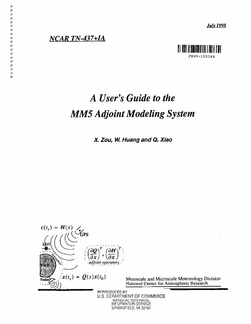
Julv 1998

NCAR TN-437+IA

PB99-155244111

A User's Guide to the

MM5 Adjoint Modeling System

X. Zou, W. Huang and Q. Xiao

E(tr) = H(x) /,I( *l'GPS

*. adjoin operators -

Q(x)x(to) Mesoscale and Microscale Meteorology DivisionNational Center for Atmospheric Research

.... ~~~~~~~~~~~~ n , ~

RFPRODUCED BYU.S. DEPARTMENT OF COMMERCE

NATIONAL TECHNICALINFORMATION SERVICESPRINGFIELD, VA 22161

p

p

p

p

p

p

p

p

p

p

p

p

p

p

p

p

p

p

p

IIl

- -, 11

=

- I),

NCAR TECHNICAL NOTES

The Technical Note series provides an outlet for a variety of NCARManuscripts that contribute in specialized ways to the body of scientificknowledge but that are not suitable for journal, monograph, or bookpublication. Reports in this series are issued by the NCAR scientificdivisions. Designation symbols for the series include:

EDD-Engineering, Design, or Development ReportsEquipment descriptions, test results, instrumentation,and operating and maintenance manuals.

IA-Instructional AidsInstruction manuals, bibliographies, film supplements,and other research or instructional aids.

PPR-Program Progress ReportsField program reports, interim and working reports,survey reports, and plans for experiments.

PROC-ProceedingsDocumentation or symposia, colloquia, conferences,workshops, and lectures. (Distribution may be limited toattendees.)

STR-Scientific and Technical ReportsData compilations, theoretical and numericalinvestigations, and experimental results.

The National Center for Atmospheric Research (NCAR) isoperated by the nonprofit University Corporation forAtmospheric Research (UCAR) under the sponsorship of theNational Science Foundation. Any opinions, findings,conclusions, or recommendations expressed in this publicationare those of the authors(s) and do not necessarily reflect theviews of the National Science Foundation.

CONTENTS_ _~~~~~~~~~~~~~~~~~~~~~~~~~~~~~~~~~~~~~~~~~~~~~~~~~~~~~~~~~~~~~~~~~~~~~~~~~~~~~~

CONTENTS

1 INTRODUCTION

1.1 Horizontal Grid Specification 1-51.2 Vertical coordinate 1-51.3 Time integration 1-51.4 Lateral boundary condition 1-5

2 Getting Started

2.1 File Naming Conventions 32.2 Code Testing 82.3 Adjoint Modeling System Source Code 10

3 MM5 Forecast

3.1 Purpose 3-33.2 Forecast Job deck 3-33.3 The Main forecast program: mm5fcst.F 3-7

4 Sensitivity Experiment

4.1 Purpose 4-34.2 The main routine of the sensitivity calculation: sens.F 4-44.3 A more general adjoint sensitivity study 4-94.4 The job deck of the sensitivity calculation: sens.deck 4-11

5 4D-VAR

5.1 Purpose 5-35.2 Physics Options in MM5's 4D-VAR System 5-45.3 Procedures to run a 4D-VAR experiment 5-55.4 Some Common Errors Associated with 4D-VAR Failure 5-95.5 A Twin 4D-VAR Experiment: 5-105.6 4D-VAR Job Deck 5-125.7 The main 4D-VAR program: mindry.F 5-185.8 The MM5 forward model subroutine incorporated with the calculation of

(cost function) and (forcing terms): mm5dry.F 5-265.9 The MM5 adjoint model subroutine incorporated with the forcing terms

(calculated in mm5dry.F): adjdry.F 5-31

6 Conclusion

6.1 Numerical efficiency 6-36.2 Observation operators 6-4

MM5 Adjoint Tutorial

I L I ,,

i

CONTENTS

6.3 Adjoint physics 6-46.4 Background information 6-5

7 References

MM5 Adjoint Tutorial

PREFACE_ * - B | ...~~~~~~~~~~~~~~~~~~~~~~~~~~~~~~~~~~~~~~~~~~~~~~~~~~~~,

Acknowledgments

This user's guide is our first attempt to compile our adjoint code into written documenta-tion, and it was not completely ready in time for our first MM5 Adjoint Model Tutorial which washeld during July 24-25, 1997. This version is completed at the time of the second MM5 AdjointTutorial being held July 28-31, 1998.

We would like to take this opportunity to thank the reviewers (Juanzhen Sun and F. Van-denberghe) for their suggestions, which have added to the document's readability as well as tech-nical accuracy, and for their willingness to complete their reviews within the minimum time theywere allowed. We would also like to specifically thank Ingrid Moore who did all the editorialwork for us.

MM5 adjin Tutoria iiiMM5 adjoint Tutorial iii

1: INTRODUCTION

INTRODUCTION- .rn . . a ak a S as A - -as - f - l a 3 e W n

Horizontal Grid Specification 1-5

Vertical coordinate 1-5

Time integration 1-5

Lateral boundary condition 1-5

MM5~c Adjin Tutoria I-1-1MM5 Adjoint Tutorial

1: iNTRODUCInON-- ._.

1-2 MM AdoiaTuora1-2 MM5 Adjoint Tutorial

1: INTRODUCTIONi i. i i i i i i i

INTRODUCTION

urNM W w a am w v am N Ia a a a a a a m W aW V a aM W at a %

During three and one-half year period from 1994 to 1997 when the first author stayed atNCAR, an adjoint mesoscale model suitable for analyzing and predicting mesometeorologicalflows was developed by the Mesoscale Prediction Group (MPG) within the Mesoscale andMicroscale Meteorology (MMM) Division of the National Center for Atmospheric Research(NCAR). It is based on the fifth-generation Penn State/NCAR Mesoscale Model (MM5, Grell etal., 1993, Dudhia, 1993). MM5 is the latest in a series that developed from a mesoscale modeldescribed by Anthes and Warner (1978) with the addition of a multiple-nest capability, nonhydro-static dynamics, and more physics options.

The MM5 modeling system is maintained by the MesoUser manager at NCAR. Wz hope thatin the near future we will have a MesoUser manager for the MM5 adjoint modeling system, whowill serve a similar role as the MesoUser manager of the MM5 modeling system, i. e., 1) main-taining a working set of programs and the accompanying set of C-shell scripts; 2) addressing andnotifying users of uncovered problems; 3) testing bug fixes to the standard package prior to gen-eral release; and 4) providing user services. Right now these duties are shared by the members inthe data assimilation subgroup within the MPG.

The current version of the MM5 adjoint modeling system and its prototype 4-dimensionaldata assimilation procedure were built on an original MM5 modeling system and executed beforethe forward model integration and after all the pre-processings of the data were done. Figure 1.1shows the general flow of the set of programs required for a typical data assimilation and the sub-sequent forecast run. The rectangular boxes in the right column of the figure represent the pro-grams that are run before an actual forward model prediction is made, and from top to bottom theyrepresent the order in which the job decks are typically run. These are the same as in the MM5modeling system. The middle part of the figure represents all of the non-conventional data, the"4D-VAR" experiments, or the sensitivity study. The forward model integration following eitherthe INTERP or adjoint experiments is basically the same as in the original MM5 modeling systemwith minor changes. The last step of post-processing is the same as that in the MM5 modelingsystem. As we can see from this flow chart, we don't have a complete 4D-VAR system, whichshall replace all the pre-processing programs in a consistent manner.

This document focuses primarily on explaining the use of the individual programs whichemploy the MM5 adjoint model. We will explain the job deck, parameter setting, and the techni-cal aspects of the code of the main programs. We will not attempt to explain the technical aspectsof other subroutines, which can be used as a black box for users anyway. There is a chapter foreach program of the adjoint system. Each of the chapters reviews the user input required for thesuccessful run and provides hints gleaned from experience. Examples with required input data are

M M I5I I TutoriI a 1-3

1-3MMS Adjoint Tutorial

1: INTRODUCTION

MSM5 `4-,2 or Adioint Sensitivity Eaeriment

Aioint cafulation M9Ž P•E-P-fOCTSSOR

Various AdditionalObservations-

Fig. 1.1 Program flow for incorporating MM5 adjoint calculations: center rectanglesdenote individual components of the modeling and assimilation system. Shaded rec-tangles represent added programs to the MM5 modeling system with the use of theMM5 adjoint model.

1-4 MM5I Ad jon Tutorial . - -- __1-4 MM5 Adjoint Tutorial

: INTRODUCTION

provided and the expected results are displayed.

The remainder of this chapter addresses some of the fundamental aspects of the MM5 model-ing system, which will potentially affect the construction and the use of the MM5 adjoint model indifferent ways. These are the vertical and horizontal grids, the time integration scheme, and thehandling of the lateral boundary conditions. Following this is chapter 2, which introduces the userto the code structure particular to the MM5 adjoint modeling system. Chapter 3 briefly describesMM5 forward model run. Chapters 4 and 5 describe the sample jobs of two sensitivity experi-ments and a "4D-VAR" twin experiment, respectively. Both of them are available to the user. Con-clusions and future planning are presented in Chapter 6.

1.1 Horizontal Grid Specification

The MM5 adjoint modeling system does not have a nesting feature. The horizontal domain isthe Arakawa B-Grid, where the horizontal wind components (u, and v) are defined on the "dot"points and the temperature, moisture, vertical velocity and pressure perturbation fields (T, qv qr,qc, w, and p') on the "cross" points. The dimension of the model grids must be set up to allow thegrid to begin and end on a dot point, which means that the total number of the grid points in bothI and J directions are odd numbers. As in the MM5, model domain is a rectangular array of gridpoints, with J-direction (x-direction) moving from the left edge to the right edge and I-direct (y-direction) from the lower edge to the upper edge.

1.2 Vertical coordinate

The model uses a, a terrain-following norlized pressure coordinate defined as(P- Ptopl/ Psfc-Ptop (1.1)

Ptop Psfcwhere is the user defined model lid (which normally is greater than 50 mb) and is thesurface pressure. The model computations are performed on the half a layers, where the values ofu,v,Tqv,qc,qr,w,and p' are taken to be representative of the respective variables through the depthof the a layer.

1.3 Time integration

The nonhydrostatic equations of MM5 are fully compressible and they permit sound waves.These are fast waves and require a short time step for numerical stability. A time-splitting schemeis applied to split these fast moving waves from the rest of the solution. Terms related to the soundwaves are separated from the slow terms, which are kept constant during the sub-steps, and a shorttime step is used to make the model more efficient. A semi-implicit scheme is used for the fastterms and a leapfrog scheme is used for the slow terms.

1.4 Lateral boundary condition

The lateral boundary conditions are brought to the model through a nudging process, except~L~ ~~YYI VYI~~J VV~VI~VLI LY VVY~~ Ir UY ~rVYV UV~~~~ · Ylf~r·

MM5 Ad oi.. --Tu- [.5

NMM Ad~joint Tutorial 1-5

1: INTRODUCTION_ i !l

for the vertical velocity and the horizontal wind at the outflow boundaries. The vertical velocitycan vary freely except for the outmost rows and columns to satisfy a zero gradient condition. Thewind values at the outflow boundaries are obtained by extrapolation from the interior points.

1-6 MM Adon Tutorial-

MM5 Adjoint Tutorial1-6

2: GETTING STARTED

GETTING STARTED3 ^ -AB n S sS t- tr i S& Va w a KS S is uS t 3 R SS us ax

File Naming Conventions 2-1

Code Testing 2-6

Adjoint Modeling System Source Code 2-7

XMAL'. A;^d;nt Trt.nri- 2-1Iflats iLUllSIIlt I Utl U l

1: GETTING STARTEDn - , _,

-2 MM5 Adon Tutorial - -MM5 Adjoint Tutorial2-2

2: GETTING STARTED

Getting Started

; a aX a ew a" * m * = m = O Wa r a a mm m Wa a

This section is for new users of the MM5 adjoint model. It is assumed that the user is familiarwith the MM5 modeling system and with the UNICOS environment.

Section 2.1 of this chapter describes the files that are currently available in the supported programdirectories. A brief overview of the standard naming convention of these files is given. Section 2.2describe a supported test capability to check the correctness of the TLM and adjoint model. Thelast portion of the chapter, section 2.3, describes how users can access the Fortran source code forthe MM5 adjoint model system.

2.1 File Naming Conventions

All of the adjoint-related calculations are controlled by job decks. The individual user-levelmodeling system programs are FORTRAN source codes that are maintained by MAKE (a Craysource code control system). MAKE allows users to save tremendous compiling time for anymodification made to the code.

The job decks and files for each component of the package are located in separate subdirecto-ries on paiute. Following is a list of the main subdirectories containing all the MM5 adjoint mod-eling system files.

* fdvar

-fdvar/Tutorial_97/adjm-fdvar/Tutorial_97/fwdm-fdvar/Tutorial_97/include-fdvar,Tutorial_97/mainfcst-fdvar/Tutorial_97/main_minimization-fdvar/Tutorial_97/main_sensitivity-fdvarfTutorial_97/main_test-fdvar/Tutorial_97/mfwm-fdvar/Tutorial_97/minm-fdvar/Tutorial_97/tglm-fdvar/Tutorial97/tstm-fdvar/Tutorial_97/utlm

To run a standard model forecast, sensitivity experiment, or data assimilation experiment,

MM5 Ajin Tutoria 2-3I- -- --2-3MM5 Adjoint Tutorial

2: GETINNG STARTED_ . _ _ __ -,- --,,__.r

users are required to make a few lines of changes in the include subdirectory and either main fcst(model forecast), or main sensitivity (adjoint sensitivity calculation), or mainminimization (4D-VAR experiment) subdirectory, respectively. Users do not need to touch the rest of the subdirecto-ries, i.e., adjm, bdym, fwdm, mfwdm, minm, tglm, utlm, and maintest. In this section, we willbriefly describe these directories which users do not need to modify. The subdirectory main testwill be explained in this section. The three main subdirectories mainfcst, main sensitivity andmainminimization will be explained in more detail in the following chapters 3-5.

The subdirectoryfwdm contains all the subroutines of the MM5 model which are listed as fol-lows:

o fwdm

-fdvar/Tutorial_97/fwdm/addall.F-fdvar/Tutorial_97/fwdm/addrx c.F-fdvar/Tutoial_97/fwdm/bdy_store.F-fdvar/Tutorial_97/fwdm/bdy_update.F-fdvar/Tutorial_97/fwdm/bdyin.F-fdvar/Tutorial_97/fwdm/bdyuv.F-fdvar/Tutorial_97/fwdm/bdyval.F-fdvar/Tutorial_97/fwdm/blkpblFl-fdvar/Tutorial_97/fwdm/cadjmx.F-fdvar/Tutorial_97/fwdm/cup.F-fdvar/Tutorial_97/fwdm/cuparal .F-fdvar/Tutorial_97/fwdm/cupara2.F-fdvar/Tutorial_97/fwdm/dots.F-fdvar/Tutorial_97/fwdm/equate.F-fdvar/Tutorial_97/fwdmexmoiss.F-fdvar/Tutorial_97/fwdm/gauss.F-fdvar/Tutorial_97/fwdm/hadv.F-fdvar/Tutorial_97/rwdm/hirpbl.F-fdvar/Tutorial_97/fwdm/init.F~fdvar/Tutorial_97/fwdm/lwrad.F-fdvar/Tutorial_97/fwdm/mapsmp.F-fdvar/Tutorial_97/fwdm/maximi.F-fdvar/Tutorial_97/fwdm/minimi.F-fdvar/Tutorial_97/fwdm/minit.F-fdvar/Tutorial_97/fwdm/minitO.F-fdvar/Tutorial_97/fwdmnmrdinit.F-fdvar/Tutorial_97/fwdmlnlmod.F-fdvar/Tutorial_97/fwdm/nudge.F-fdvar/Tutorial_97/fwdm/outprt.F-fdvar/Tutorial_97/fwdm/output.F-fdvar/Tutorial_97/fwdm/outsav.F-fdvar/Tutorial97/fwdmlouttap.F-fdvar/Tutorial_97/fwdm/p 1p2.F-fdvar/Tutorial_97/fwdm/param.F-fdvar/Tutorial_97/fwdm/pwater.F-fdvar/Tutorial_97/fwdm/conadv.F

2-4 MM Adon TutorialMM5 Adjoint Tutorial2-4

2: GETTING STARTED-~~~

-fdvar/Tutorial_97/fwdm/conmas.F-fdvar/Tutorial_97/fwdm/convad.F-fdvar/Tutorial_97/fwdm/decpu.F-fdvar/Tutorial_97/fwdm/deltatim.F-fdvar/Tutorial_97/fwdm/diffu.F-fdvar/Tutorial_97/fwdm/diffut.F-fdvar/Tutorial_97/fwdm/rdinit.F

fdvar/Tutorial_97/fwdm/set_assign.F-fdvar/Tutorial_97/fwdm/sfcrad.F-fdvar/Tutorial_97/fwdm/skipf.F-fdvar/Tutorial_97/fwdm/siab.F-fdvar/Tutorial_97/fwdm/solarl .F-fdvar/Tutorial_97/fwdmlsolve3.F-fdvar/Tutorial_97/fwdm/sound.F-fdvar/Tutoria_97/fwdm'swrad.F-fdvar.Tutorial_97/fwdm/tmass.F-fdvar/Tutorial_97/fwdm/ua2ueb.F-fdvar/Tutorial_97/fwdm/vadv.F-fdvar/Tutorial_97/fwdmlvtran.F-fdvarlTutorial_97/fwdmlwbc.F-fdvar/Tutorial_97/fwdm/xa2xb.F

We can see that most of the subroutines are copied from the MM5 modeling system except the

subroutines ua2ueb.F, xa2xb.F, bdy_update.F and wbc.F. All of these are needed from the fact thatfor a model to be used in an optimization procedure, only the independent input variables shouldbe viewed as the control variables of the model. (see Zou et al., 1997). The subroutine ua2ueb.Fputs the initial condition (IC) near the lateral boundary to its corresponding boundary values;xa2xb.F gives the UA, VA, ... values to UB, VB, ... ; bdy_update.F calculates values of the lateralboundary conditions (LBC) for UEB, UWB, ..., etc at the next LBC time from its previous valuesof UEB, UWB, ..., and their boundary tendencies; and wbc.F calculates the vertical velocity atboth the bottom and top of the model from other variables, and is part of the calculation originallydone in the pre-process stage in the MM5 modeling system.

The subdirectory tglm includes all the linearized subroutines corresponding to each of thenonlinear subroutines in the subdirectory fwdm. The linearized files have a standard naming con-vention. The first letter of the subroutine is always "L", followed by the same name as in the MM5forward model (those files in the subdirectory fwdm).

tglm

-fdvar/Tutorial97/tglm/lbdyval.F-fdvar/Tutorial_97/tglm/lblkpbl.F-fdvar/Tutorial_97/tglm/lcadjmx.F

fdvar/Tutorial_97/tglm/lconvad.F-fdvar/Tutorial_97/tglm/ldecpu.F-fdvar/Tutorial97/tglm/ldiffu.F-fdvar/Tutorial_97/tglm/ldiffut.F-fdvar/Tutorial 97/tglm/lgauss.F-fdvar/Tutorial_97/tglm/lhadv.F

MM5 Adjoint Tutorial 2-5

2: GETTING STARTED

-fdvar/Tutorial97/tglm/lsfcrad.F-fdvar/Tutorial_97/tglm/lslab.F-fdvar/Tutorial_97/tglm/lsolve3.F-fdvar/Tutorial_97/tglm/lsound.F-fdvar/Tutorial_97/tglmllvadv.F

The total number of files in tglm is much less than that in fvdm, since the same subroutines,which are linear, will be used in the TLM. To make this happen, we have kept the same variablenotation for perturbation fields in TLM as in the nonlinear model, and the basic state variables areappended by a number "9".

All the adjoint subroutines are kept in the subdirectory adjm. For each subroutine in MM5,there is an adjoint subroutine with the first letter being "A" followed by the same name as in theMM5. For instance, the adjoint subroutine ahadv.F is simply the transpose of the linearized sub-routine lhadv.F of hadv.F, realized at the coding level. The adjoint variables have the same namingconvention in the code as their corresponding variables in the MM5 or their perturbation variablesin the TLM. Following is a list of the subdirectory adjm:

adjm

-fdvar/Tutorial_97/adjm/abdyupdate.F-fdvar/Tutorial_97/adjm/abdyuv.F-fdvar/Tutorial_97/adjm/abdyval.F-fdvar/Tutorial_97/adjm/ablkpbl.F-fdvar/Tutorial_97/adjm/acadjmx.F-fdvar/Tutorial_97/adjm/aconvad.F-fdvar/Tutoria!l97/adjm/adecpu.F-fdvar/Tutorial_97/adjm/adiffu.F-fdvar/Tutorial_97/adjm/adiffut.F-fdvar/Tutorial_97/adjm/aequate.F-fdvar/Tutorial_97/adjmiagauss.F-fdvar/Tutorial_97/adjm/ahadv.F-fdvar/Tutorial_97/adjm/anudge.F-fdvar/Tutorial_97/adjm/apwater.F-fdvar/Tutorial_97/adjmnasfcrad.F-fdvar/Tutorial_97/adjm/aslab.F-fdvar/Tutorial_97/adjm/asolarl .F-fdvar/Tutorial_97/adjm/asolve3.F-fdvar/Tutorial_97/adjm/asound.F-fdvar/Tutorial_97/adjm/avadv.F-fdvar/Tutorial_97/adjm/awbc.F

Both TLM and the adjoint model are linear models, which are all linearized around the non-linear model solution. The basic principles we adapted in MM5 TLM and adjoint model develop-ment for calculating the nonlinear coefficients are as follows:

The model predictions at every time step, consisting of wind, temperature, specific humidity,cloudwater, rainwater, and pressure perturbation, were saved and used as the only input basic stateinformation. The nonlinear coefficients in the TLM and adjoint model are all recalculated from

2- MM Adjin Tutorial

MM5M Adjoint Tutorial2-6

2: GETtING STARTED,I _., , , _ ..

them.

Also, for every subroutine, we assume that the input variables and their basic state values areavailable and consist of all the input data for that subroutine. This way each of the subroutinesbecomes a relatively independent piece of code in developing and checking its tangent linear andadjoint code and linking them together. Since all the basic state variables are appended by "9",there is a need to generate another set of subroutines for the basic state calculation in the TLM andadjoint model if these subroutines in the nonlinear model produced some values which were usedin the future calculation of the nonlinear coefficients in the TLM and adjoint model. These sub-routines are assembled in the subdirectories mfwm, which is listed as follows:

c mfwm

-fdvar/Tutorial_97/mfwm/mbdyuv.F-fdvar/Tutorial_97/mfwm/mbdyval.F-fdvar/Tutorial_97/mfwm/mblkpbl.F-fdvar/Tutorial_97/mfwm/mconadv.F-fdvar/Tutorial_97/mfwm/mconmas.F-fdvar/Tutorial_97/mfwm/mconvad.F-fdvar/Tutorial_97/mfwm/mdecpu.F-fdvar/Tutorial_97/mfwm/msfcrad.F-fdvarlTutorial_97/mfwm/mslab.F-fdvar/Tutorial_97/mfwm/msound.F

Notice that all the subroutines in mfwm subdirectory start with a letter "M", followed by thesame subroutine name in the MM5. For instance, subroutine mblkpblF is the same as blkpbl.F inthe subdirectory fwdm except that the input and output variables of blkpbl.F are appended with"9" in mblkpb.F. The local variables in mblkpbl.F are still the same as in blkpbl.F

Having all the codes for the MMS, its TLM and its adjoint model, we now move to the codefor the minimization procedure. The subdirectory minm contains all the subroutines for the lim-ited-memory quasi-Newton method (Zou et al., 1993). Following is a list of them:

* minm

-fdvar/Tutorial_97/minm/ddot.F-fdvar/Tutorial 97/minm/lmcheck.F-fdvar/Tutorial_97/minm/lmdir.F-fdvar/Tutorial_97/minm/lmprint.F-fdvar/Tutorial_97/minm/lmstep.F-fdvar/Tutorial_97/minnVval 5ad.F-fdvar/Tutorial_97/mninm/val 5bd.F-fdvar/Tutorial 97/minrrval 5cd.F-fdvar/Tutorial 97/minnmvdO5ad.F-fdvar/Tutorial_97/minm/vd05bd.F-fdvar/Tutorial_97/minm/verigr.F

In the minimization code, one dimensional arrays are used for the contral variable, gradient,

MM5 Adjoint Tutorial 2-7MM15 Adjoint Tutorial 2-7

2: GETTING STARTED,.. _ ,, _ _

and so on, it is necessary to convert the multi-dimensional variables in the model into one dimen-tional variable. The subroutines for data transfer from multi-variables and multi-dimensions toone dimensional array and back, along the weighting and scaling, the direct access of data, theinteractive mass storage usage and so on, are included in the subdirectory utlm.

* ulm

-fdvar/Tutorial_97/utlmladd_variabie.F-fdvar/Tutorial_97/utlmnaget.F-fdvarTutorial_97/utlm/agetO.F-fdvarJTutorial_97/utlm/aput.F-fdvar/Tutorial_97/utlm/aputO.F-fdvar/Tutorial_97/utlm/aremovenegative.F

fdvar/Tutorial_97/utlm/astart.F-fdvar/Tutorial_97/utlm/averg.F-fdvar/Tutorial_97/utlm/bas_appro.F-fdvar/Tutorial_97/utlm/bas_approw.F-fdvar/Tutorial_97/utlm/diff_variable.F-fdvar/Tutorial_97/utimlmaxdiff.F-fdvar/Tutorial_97/utlm/maxdiffb.F-fdvar/Tutorial_97/utlm/oned.F-fdvar/Tutorial_97/utlm/plp2.F-fdvar/Tutorial_97/utlm/pmwgt.F-fdvar/Tutorial_97/utlm/rcvr_rst.F-fdvar/Tutorial_97/utnlmremovenegative.F-fdvar/Tutorial_97/utlm/save_rst.F-fdvar/Tutorial_97/utlm/scaling.F-fdvar/Tutorial_97/utlm/scalingb.F-fdvar/Tutorial_97/utlm/trans_bas.F-fdvar/Tutorial_97/utlm/transf.F-fdvar/Tutorial_97/utlm/transfb.F-fdvar/Tutorial_97/utlm/transfbgrad.F-fdvar/Tutorial_97/utlrr/transhir.F-fdvar/Tutorial_97/utlm/weight.F-fdvar/Tutorial_97/utlm/write_mss.F-fdvar/Tutorial_97/utlm/zero_variable.F

All the code listed above does not need to be modified for different case studies and differentadjoint applications.

2.2 Code Testing

The correctness of the MM5 TLM and adjoint model can be tested by a Taylor formula and analgebraic expression, respectively (see (3.15) in Zou et al. 1997). We provided this testing code inthe subdirectory main_adjointtest.

The job deck tgl.deck will carry out a TLM test. For an arbitrarily selected predicted variable,the value of its perturbation prediction obtained by TLM should approach the NLM predicted val-

2- MM5 Adon TutorialMM5 Adjoint Tutorial2-8

2: GET1TNG STARTED

ues linearly as the order of magnitude f the initial perturbation ecreases. This will show a list ofresults in the output file as follows:

Tr(a) +q(a)

0. 172015E 10.6802895E+10.1146562E+20.1000003E+10.1000002E+10.1000001E+l0.IOOOOO1E+10. l0001OE+10.1000002E+l0.9999699E+00.9999190E+00.1001545E+l0.1053077E+10.8635745E+1

0.1295176E+10.5621636E+10.1018204E+20.1000012E+10.1000004E+i0.1000003E+10.1000003E+10.1000003E+10.1000002E+l0.9999728E+00.9999589E+00.1000918E+10.1021803E+10.6896338E+1

0.1845927E+10.3591716E+20.8753406E+20.9999943E+00.9999994E+00.9999997E+00.9999997E+00.9999993E+00.9999973E+00.9999809E+00.9998853E+00.1004275E+10.1207661E+10.2222289E+2

0.5209394E+10.1351556E+30.8990221E+30.9999410E+00.9999952E+00.1000OOOE+l0.1000000E+l0. 100000E+l0.9999975E+00.1000045E+10.9996812E+O0.1002713E+10.1111543E+10.6861195E+1

The above results were obtained by running the standard case for a 3-h prediction of zonal windcomponent, meridional wind component, temperature and specific humidity. The standard case isthe same case chosen for the MM5 tutorial since 1997. It is set up to make a 24-h forecast for thetime period 0000 UTC 13 to 0000 UTC 14 March 1993 at a very coarse resolution (120 km) witha grid size of 26 x 31 x 10. The values of a varies from 103 to 10-16. h is taken as the vector ofthe initial condition. Physical options include the grid-resolvable precipitation, the Kuo cumulusprecipitation, the bulk PBL and surface flux. All the test and experimental results in this userguide are obtained using the same version of the MM5 forward model, the corresponding tangentlinear model and adjoint model.

The job deck adj.deck will run the adjoint test. A correct adjoint code means that the two num-bers (Wright and Wleft represent the values of the right- and left-hand-side of the algebraic for-mula (3.16) in Zou et al. (1997)) are the same with 13 digit accuracy on a 64-bit machine.Exception when less digits could be obtained even with an actually correct code may occur, whichwas discussed in Zou et al. (1997). An example of the correctness check of the adjoint model isshown below:

Wright = 0.13519434210906E+17Wleft = 0.13519434210906E+17

which was obtained by running the standard case for a 3-h time integration. It includes the 3-hprediction of all the model fields. Since no normalization was done, such a test may be misleadingfor the fact that some of the quantities (say T or p') may be several orders of magnitude biggerthan others (say u, v) and a correct test may just mean that the largest term is correct. A more stricttest is to test different variables separately. For example, we can test only the wind fields (u, v)and we obtain:

Wright = 0.53709592507228E+13Wleft = 0.53709592507228E+13

MM Adon Tuora 2-9


2: GETTING STARTEDwS,

_ __

or we can make a test to the pressure perturbation (p'):

Wright - 0.13512767057137E+17Wleft = 0.13512767057137E+17

We observe that if there is a bug in the adjoint model which affects the wind fields and results inonly a 10 digit accuracy, it won't be reflected in a test which includes all the model fields.

Users are advised to make their own TLM and adjoint tests for their new cases before makinga productive sensitivity or data assimilation experiment. For the latter, a gradient check is alsonecessary, which will be discussed in Chapter 5.

2.3 Adjoint Modeling System Source Code

The standard version of the MM5 adjoint modeling system can be copied from the NCAR craypaiute or read from the mass storage file. They are listed as

paiute: -fdvar/Tutorial_97/MM5_ADJ.tar.gzor

mass storage: /FDVAR/TUTORIALMM5_ADJ.tar.gz

Users just need to execute two commands: gunzip MM5_ADJ.tar.gz and tar -xvf MMS_ADJ.tarto get the standard source code after the files are copied to their local machine.

Remark:

A detailed description of the Make utility and the job deck syntax is given in Chapters 2 and 3 ofthe "PSU/NCAR Mesoscale Modeling System Tutorial Class Notes.".

2-1 MiM Adjin TutorialMM5 Adjoint Tutorial2-10

3: MM5FCST

MM5FCSTI mua aml - t a o ag a a a a . NM I m ~ a mA _ .

Purpose 3-3

Example of mm5fcst.F 3-4

MM5 Adjin Tuora 3-I II


3: MM5FCSTI il

3-2 MM Adjin Tutorial_ _3-2 MM5 Adjoint Tutorial

3: Forecast

MM5 Forecast

it O am Mt a a= Am - - an =a a= aI " Am = NM 4= =X a m a

3.1 PurposeThis chapter describes how to do a straight-forward model integration. Users have a choice to

use the standard MM5 modeling system to run the forecast or to use the code consistent with theMM5 adjoint model. If it's the latter case, users can carry out the forward MM5 model forecast inthe subdirectory mainfcst, which contains only two files:

main fcst

-fdvar/Tutorial_97/mainfcst/fcst.deck-fdvar/Tutorial_97/mainfcst/mm5fcst.F

3.2 Forecast Job deck

The job deck fcstdeck is a C-shell script and executes a forward model run using codes(mmSfcst.F) consistent with the MM5 adjoint model. It is set up to make a 24-h forecast startingeither from the standard MM5 input initial condition or the "optimal" initial condition obtainedby a minimization procedure. The user may define shell variables that are expanded for use as filenames, directories, or titles for output files. Users with syntax questions for C-shell constructs arereferred to the man pages for "csh".

The job deck is structured similarly to the job decks in the MM5 modeling system, i.e., onecan choose different physics options, set the IC and LBC, and output the forecasts at the desiredtime interval. There are only two parameters in the job deck which may need further explanation:parameter IFWDRUN and LRGPRE. The parameter IFWDRUN=O means to make a forecastfrom the standard MM5 IC file, and IFWDRUN=l means that one wants to make a forecast froman optimal IC (output from a 4D-VAR nrn) which is formatted as

OPEN (UNIT=91 FORM='UNFORMATTED',STATUS='UNKNOWN')READ (91) UAVA,TA,QVA,PPA,WA,QCA,QRACLOSE(91)

FDVA Tuora 3-3 ~ -~- r _ ' -- ---- ' - -3-3FDVAR Tutorial

3: Forecast

The parameter LRG_PRE controls whether or not to include the large-scale precipitation pro-cess. We added this parameter in case one wants to examine the moisture "on-off' problem. In thefollowing we enclose the job deckfcst.deck.

* fcst.deck

# QSUB -r FCST # request name# QSUB -q reg # job queue class prem econ#QSUB -eo ## QSUB -o fcst.out # stdout and stderr together# QSUB -IM 8Mw # maximum memory# QSUB -IT 5000 # time limit# QSUB # no more qsub commands#ja

#set echo

# * ****** *****+ ***** ***t***** ******************tt

# ******* 4dvar batch C shell *****# *****t**$*******************************$***

# set Data_Dir = /Models/zou/TUTORIALIFDVAR/dataset Work_Dir /Models/zou/tmp-fcstset CurtDir= 'pwd'cd $Work_Dir

#set Recompiled - Yes # recompile the codeset Recompiled = No

## type of 4dvar job#set IFWDRUN = # 0 -> From analysis, 1 -> From Optimal IC

## local namelist values#cat >! mmlif << EOF&FDPARAMIFWDRUN = $IFWDRUN, ; 0-> From analysis, 1 -> From Optial IC

LRG_PRE = , ; 0,1 large-scale precipitation

&OPARAM ; <-- MOD2

; YOU CAN REMOVE THE UNWANTED DATA FROM THE FOLLOWING LISTING; AND USE THE DEFAULT VALUES DEFINED IN SUBROUTINE 'PARAM'.

IFREST = F, ;RESTARTIXTIMR =720,

LEVIDN = 0,; level of nest for each domainNUMNC 1, ; ID of mother domain for each nestIFSAVE = F, ; SAVE DATA FOR RESTART

SAVFRQ 180., ; ... in minutes.IFTAPE = 1, ; OUTPUT FOR GRIN backend

TAPFRQ =60., ; ... in minutes.IFPRT = 1, ; do not change

-4. FDA Tutorial3-4 FDVAR Tutorial

3: Forecast

PRTFRQ = 180., ; Print output frequency in minutesMASCHK = 30, ; MASS CONSERVATION CHECK (minutes)

&LPARAMiactiv 1,0,0,0,0,0,0,O,O,O,; in case of restart: was this domain active?

;************ start physics options ***************

IFRAD - 0, ;RADIATION COOLING OF ATMOSPHERE - 0, 1, 2RADFRQ =30., :RADIATION FREQUENCY IN MINUTESICUSTB = 1, ;STABILITY CHECK FOR CUMULUS PARAM. - 0(no stab. check), 1IEXICE 0, ;ICE-PHYSICS IN EXPLICIT SCHEME - 0, 1IFDRY = 0, ;FAKE-DRY RUN - 0, 1IMVDIF = 0, ;MOIST VERTICAL DIFFUSION IN CLOUDS - 0, 1IBMOIST =0, ;BOUNDARY AND INITIAL WATER/ICE SPECIFIED -.0, 1ICOR3D - 1, ;3D CORIOLIS FORCE- 0,IFUPR = 0, ;UPPER RADIATIVE BOUNDARY CONDITION - 0, 1

IBOUDY 3,2, 2, 2, 2, 2, 2, 2, 2,2, ;BOUNDARY CONDITIONS - 0, 1, 2, 3, 4

IBLTYP = 1,2,2,2 2,2,2, 2, 2, 2,;PBL TYPE- 0, 1, 2IDRY - 0, 0,0, 0, ,0,0,0,0, O, ,;MOIST OR DRY CASE - 0, 1IMOIST= , 1,, 1, 1, 1, 1, 1, 1, ;NON-EXPLICIT, EXPLICIT, - 1, 2ICUPA =2, 1, 1, 1, 1, 1, 1, 1, 1,;NONE,KUO,GRELL,AS - 1,2,3,4ISFFLX= , , 1,, 1, 1, 1, 1, 1, ;SURFACE FLUXES - 0,ITGFLG 1, 1, 1, 1, 1, 1, 1, 1, 1,;SURFACE TEMPERATURE- 1, 3ISFPAR = 11, 1, 1, ,1, 1, 1, , 1;SURFACE CHARACTERISTICS - 0, 1ICLOUD = 1, 1, 1,1,, 1, 1, 1, 1,;CLOUD EFFECTS ON RADIATION - 0, 1ICDCON = 0, 0, 0, 0, 0, 0, 0, 0, 0,, ;CONSTANT DRAG COEFFICIENTS - 0, 1

IFSNOW = 0, , 0, 0, 0, 0, 0, 0,, 0,;SNOW COVER EFFECTS - 0, 1IMOIAV = 0, 0, 0, 0, 0, 0, 0, 0, ,;VARIABLE MOISTURE AVAILABILITY - 0, 1IVMIXM 1, 1, 1, 1,1, 11,, 1, 1, ;VERTICAL MIXING OF MOMENTUM - 0, 1HYDPRE= 1.,1.,i.,1.,1.,1.,1 .,1.,1.,.,;HYDRO EFFECTS OF LIQ WATER - 0., 1.IEVAP = 1, 1, 1,1, 1,1,11,1, 1, ;EVAP OF CLOUD/RAINWATER - <0, 0, >0ISHALLO= 0, ,0 00, 0, 0, 0, ;SHALLOW CONVECTION - 0, 1

;************* end physics options **************

;************* start nesting options **************

nestix = 26, , 46, 46, 4 46, 4 6, 46, 46,; domain size Inestjx=31, 61, 61, 61, 61, 61, 61, 61, 61, 61,; domain sizeJnesti = 1, 1, 1, 1, 1, 1, 1, 1, 1, 1,;startlocationInestj = 1, , 1, 1, 1, 1, 1, 1, 1, 1 ,; startlocationJxstnes = 0., 0., 0 ., 0, 0., 0. 0., ., 0., 0.,; domain initiationxennes 1 440.,720.,720.,720.,720.,720.,720 .,720.720.20.,; domain completionioverw= 0, 0, 0, 0, 0,, 00, 0, 0, ; overwritedomain

-************ end nesting options ****************

&PPARAMTIMAX = 1440., ; IN MINUTES. 720=12h, 1440=24h, 2160=36h, 2880=48hZZLND = 0.1, ; ROUGHNESS LENGTH OVER LAIND IN METERS

FDVAR u oi a -_3-5FDVAR Tutorial

3: Forecast

ZZWTR - 0.0001,; ROUGHNESS LENGTH OVER WATER IN METERSALBLND 0.15, ; ALBEDOTHINLD 5 0.04, ; SURFACE THERMAL INERTIALXMAVA = 0.3, ; MOISTURE AVAILABILITY OVER LAND AS A DECIMAL

~; FRACTION OF ONECONF 1.0, ; NON-CONVECTIVE PRECIPITATION SATURATIONTISTEP = 360., ; COARSE DOMAIN DT IN MODEL, USE 3*DXifeed 3, ; OLD FEEDBACK, NO/LIGHT SMOOTHING IN FEEDBK - 1,2,3iabsor = 0, ; SPONGE ON UPPER BOUNDARY - 0,1

&FPARAM

EOF

I 1 111 5 11 to OF1 1pi tl o I*I 11 11 if A l 11d 1S 111f 1s E f] s l 1 11 at A l a t 11 11 J i t I I 11 11 llt I1t Si go Ed l I i t la 1 E1 1E E11 1 L I f I t 1 S1 I it Ji s ut 1 t iu i

Eld o t lIi a s i t I s t i J N l is. 1,1L 111 t 11 Itl Si Is 11 11 u f111 1,i 11111 111 f i f J

1,,1,,1, ,IIiiun,;,iiu;1isI END USER MODIFICATION IHJ a t Hf.lsIt t i I l ii iifis t i sgI sRs o t f it nit ON ilS 1f iE Ia / 111 h f21 I la is Iifii ii tt isi I 11 oo II l l i f11711If1 11115 Ed 1toSi 1Si Ititof Itla s it It is if PI At of is of of is II IN so if OF 11 91 of la 11 11 if 91 is 1 is It II Is 51 1s1 Ils 1s11 Iisis ifto1IIgo5solIs # to1 5 it5 is r o1f r It ofr so1 so 1

## initializations, no user modification required#set LETTERS =(A B CDEFGHIJKLMNOPQR STU V WX YZ)set FDvarUser = -mesouser/MM5V /MM5#if ( $Recompiled = Yes ) then

#makemswrite -t 1000 mm5fcst.exe $OutMM/mm5fcst.exels -

elsemsread mm5fcst.exe $OutMM/mm5fcst.exechmod +x mm5fcst.exe

endif## set up fortran input files for the forecast#nn fort.*In -s mmlif fort.7In -s $DataDir/bdyout fort.9In -s $DataDir/guess_input_kl4dvar.o fort. 11

# In -s $DataDir/guess_input_d4dvar fort. 11In -s $Data_Dir/DirObs_k!4dvar fort.20#execute:

## run FDVAR

date In -s $Curt_Dir/mm5fcst.exe.timex nice mm5fcst.exe >&! $Curt_Dir/mm5fcst.print.out

#

3-6 FDA Tutorial ,_FDVAR Tutorial3-6

3: Forecast_ _ __ _ __. __ ~~~~~~~~~~~______ __~~~~�. ~__~_ . .

3.3 The Main forecast program: mm5fcst.F

About mm5fcst.F, we mention two points: (1) the variable MAXSTP isthe total time-steps forthe entire forecast duration calculated from the value of TIMAX, whose value was set in the jobdeck; and the call to subroutine REMOVE_NEGATIVE, which is needed if the optimal IC isobtained without a specific constraint that the moisture variables qv should always be positive. Inthe following we enclose the main routine mm5fcst.F:

PROGRAM MMSFCSTcccccccccccccccccccCCCCCCCCCCCcccccccccc CCCCcc ccccccccccccccCCC Forward forecast from MM5 analysis or "optimal" ICCcccccccccccccccccccccccccccccccccc ccccccccccccccccccccccccccCCCCCCCCC# include <parame.incl># include <parmin.incl># include <param2.incl># include <param3.incl># include <addr0.incl># include <various.incl># include <point2d.incl># include <dusolvel.incl># include <variousn.incl># include <point3d.incl># include <pointbc.incl># include <nonhyd.incl># include <nonhydb.incl># include <bcontrol.incl># include <minim.incl># include <obsdata.inci>C

DIMENSION AUA(MIX, MJX, MKX),AVA(MIX, MIX, MKX),- ATA(MIX, MJX, MKX),AQVA(MIX, MJX, MKX),- AWA(MIXNH,MJXNH,KXP1NH),APPA(MIXNH,MJXNH,MKXNH),- ATGA(MIX,MJX), ARAINC(MIX,MJX), ARAINNC(MIX,MJX)

DIMENSION AQCA(MIXM, MJXM ,MKXM), AQRA(MIXM ,MJXM ,MKXM ),- AQIA(MIXIC,MJXIC,MKXIC)AQNIA(MIXIC,MJXIC,MKXIC)

C

COMMON /IEXCMN/ IEXEC(MAXNES)DIMENSION IERR(2)COMMON /LRG_PRECIPITATION/LRG_PRELRG_PRE=lREAD (7,FDPARAM)PRINT FDPARAM

CC- INITIALIZE TO ZEROC

DO 1 N=1,MAXNESDO 1 I=1,IHUGE

ALLARR(I,N)=0.

Fl/A Tuora 3-7_ ___ _.FDVAR Tutorial 3-7

3: Forecast_

----

1 CONTINUEDO 2 N=1,MAXNESDO 2 I=1 ,MIXDO 2 J=1,MJX

XNUU(U,N)=0.XMUU(IJ,N)-0.XNUT(I,J,N)=O.XMUT(IJ,N)=O.

2 CONTINUECC-- FIRST THINGS FIRST: PRESET ADDRESS OF ALL VARIABLESC-- FOR ALL NESTS.C

NSTTOT=1CALL ADDALL

CC-- NITIALIZE NUMBER OF ACTIVE NESTS AND TOTAL POSSIBLEC-- NESTS TO ZEROC

DO 4 N= 1,NLNESDO 4 NN=1 ,MAXNES

NUMLV(N,NN)=O4 CONTINUE

CC- FILL COARSE DOMAIN VARIABLES WITH DOMAIN (1)C

CALL ADDRXIC(iAXALL(1,1))CC--SET UP PARAMETERS:C

DO 5 NN=1,MAXNESIEXEC(NN)=1LEVIDN(NN)=ONUMNC(NN)=0

5 CONTINUEIF(MAXNES.EQ. 1 )THEN

PRINT *,'**I ******* ***** ONE DOMAIN ONLY! ! ***********'

ELSEPRINTr *

I '******************* MULTI LEVEL RUN!!! **********'PRINT *,

1 '**«************* ;,MAXNES,' DOMAINS TOTAL *******'

ENDIFCC-- READ IN PARAMETERS AND NAMELISTSC

CALL PARAM(IEXEC)C READ IN SUBSTRAT TEMPERATURE:C

READ(9) TMNCALL SKIPF (9,1,IERR)

CC READ IN THE BOUNDARY CONDITIONS:

3-8 FDARTuora

FDVAR Tutorial3-8

3: Forecast,, ~ ~ ~ ~ ~ ~ ~ ~ ~ ~ ~ ~ ~ ~ i

CCALL BDYIN(9,TBDYBE ,BDYTIM ,ILJL,IBMOIST)

CC obtained values of UEBC,UEBCT.......CC---- READ IN THE COARSE GRID INITIAL CONDITIONSC

CALL MRDINIT(11 ,ILJL,0)CC obtained values of UA,VA,.....WAC

CALL MINITO(IEXEC,ILJL)CC obtained values of 2-D fieldsC

IF (IFWDRUN .EQ. 1) THENOPEN (UNIT=91,FORM='UNFORMAlTED',STATUS='UNKNOWN')READ (91) UA,VA,TA,QVA,PPA,WA,QCA,QRACLOSE(91)CALL REMOVE_NEGATIVE(QVA,QCA,QRA,QIA,QNIA,IEXMS,IICE,

~- MIX,MJX,MKX,MIXM,MJXM,MKXM,MIXIC,MJXIC,M C,~- IQINDX,IQCIRINQIDXIQIINDX ,IQNIINDX)

ENDIFC

NBAS = NINT(TIMAX*60JDT )+lDTIN=DTMAXSTP-NBAS-1print*,'DT,TLMAXIAXSTP=',DT,TIMAXMAXSTP

CCPUTIN=SECOND()CALL NLMODCPUTOUT=SECOND()print*,'NLMOD CPU TIME=', CPUTOUT-CPUTIN

C88888 STOP 88888

END

FDA Tuora 3-9-I -3-9FDVAR Tutorial

3: Forecast-~~~~- -

3-10 EDVA Tutorial -FDVAR Tutorial3-10

4: SENSITIVITY

SENSITIVITYa Wu a Mas a o a = s a W mm Wa NBW smmU aMNg Aa n W

Purpose 4-3

Example of sens.F 4-4

MM5__ Adjin Tuoral4-MM5 Adjoint Tutorial 4-1

4: SENSITIVITY

MM Adjin Tutria 4 -2 -I II


4: SENSITIVITYS ~ ~ ~ ~ ~ ~ ~ , , _ _

Sensitivity Experiment

- N a s WM s a ... NS E s sa-w n - M saM n aBW M aM Me affi a N

4.1 Purpose

This chapter describes how to run an adjoint sensitivity experiment. The example we provide herecalculates the sensitivity of the 12-h forecast of the temperature in the black box in figure 4.1. Theresponse function can thus be expressed as

R(xo) = T(il,, k) k = 10,t = 12h (4.1)

wherel = land i I = 19.

Given x 0 , the sensitivity of R with respect to xO can be obtained by running the forward MM5for 12 h, which provides the basic state trajectory for the following-up adjoint model integration,i.e., running the adjoint model backward with the "initial" condition at the time t=12 h as

adi(= 12 h) = aR (4.2)axt = 12h

where x represents all the adjoint model variables at the time t=12 h. From (4.1) we obtain that

a{dj k = 10, i = 11, i = 19T (t= 12h) o { hrw i = 1(4.3)

(p otherwise

The value of Xa i(t=0) obtained by sucn an adjoint model backward integration at time t=O isthe sensitivity field. It was saved as

OPEN(UNT=91 ,FILE='GRAD.D ,FORM='UNFORMATTED',- STATUS='UNKNOWN')

WRITE(91) UAA,VAWA,TA,QVA,PPA

AA;r int Tttnrial 4-3J UJVIIlt AUtUlJUa

4: SENSITIVITY

CLOSE (91)

in the main routine.

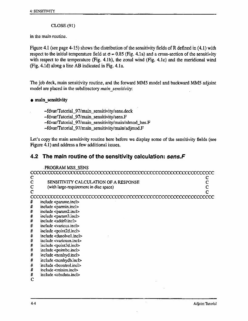
Figure 4.1 (see page 4-15) shows the distribution of the sensitivity fields of R defined in (4.1) withrespect to the initial temperature field at a = 0.85 (Fig. 4.la) and a cross-section of the sensitivitywith respect to the temperature (Fig. 4.1b), the zonal wind (Fig. 4.1c) and the meridional wind(Fig. 4. d) along a line AB indicated in Fig. 4. a.

The job deck, main sensitivity routine, and the forward MM5 model and backward MM5 adjointmodel are placed in the subdirectory main_sensitivity:

mainsensitivity

-fdvar/Tutorial_97/main_sensitivity/sens.deck-fdvar/Tutorial_97/main_sensitivity/sens.F-fdvar/Tutorial_97/main_sensitivity/main/nlmod_bas.F-fdvar/Tutorial_97/main_sensitivity/main/adjmod.F

Let's copy the main sensitivity routine here before we display some of the sensitivity fields (seeFigure 4.1) and address a few additional issues.

4.2 The main routine of the sensitivity calculation: sens.F

PROGRAM MSSSENSCCCCCCCCCCCCCCCCCCCCCCCCCCCCCCCCCCCCCCCCCCCCCCCCCCCCCCCCCCCCCCC CC SENSITIVITY CALCULATION OF A RESPONSE CC (with large-requirement in disc space) CC CCCCCCCCCCCCCCCCCCCCCCCCCCCCCCCCCCCCCCCCCCCCCCCcCCCCCCCCCCCCCCCC# include <parame.incl># include <parmin.incl># include <param2.incl># include <param3.incl># include <addr0.incl># include <various.incl># include <point2d.incl># include <dusolvel.incl># include <variousn.incl># include <point3d.incl># include <pointbc.incl># include <nonhyd.incl># include <nonhydb.incl># include <bcontrol.incl># include <minim.incl># include <obsdata.incl>C

-4 Adjin Tutoria4-4 Adjoint Tutorial

4: SENSITIVTY~~~~~~~~~~~~~~~~~~~~~~~~~~~~~~i 1

DIMENSION AUA(MIX, MJX, MKX),AVA(MIX, MJX, MKX),- ATA(MIX, MJX, MKX),AQVA(MIX, MJX, MKX),- AWA(MIXNH,MJXNH,KXP 1N H),APP.A(MIXMJXNH,MKXNH),- ATGA(MIX,MJX), ARAINC(MIX,MJX), ARAINNC(MIX,MJX)

DIMENSION AQCA(MIXM, MJXM ,MKXM), AQRA(MIXM ,MJXM ,MKXM),- AQIA(MXIMC,MJC,MKXIC),AQNIA(MIXIC,MJXIC,MKC)

C

CCOMMON /IEXCMN/ IEXEC(MAXNES)COMMON /LRG_PRECIPITATION/LRG_PREDIMENSION IERR(2)INTEGER TRIMLEN, MSSPATH_LEN

CCAAAAAAAAAAAAAAAAAAAA

CICOEFFNT=1NCEP_WEIGHT-0LRG_PRE=1

CMSSPATH = 'TMPDIR005FEBTOSAVE YOUR RUNTINME FLES/'MSSPATHLEN = TRIMLEN(MSSPATH)

CIF(MSSPATH(LEN_MSSPAT:LEN_MSSPATH) .NE. '/') THEN

LEN_MSSPATH LEN_MSSPAT ESSTH + 1MSSPATH(LEN_MSSPATH:LEN_MSSPATH) = ''

ENDIFCCv,^

CREAD (7,EDPARAM)PRINT FDPARAM

CC--- NITIALIZE TO ZEROC

DO I N=I,MAXNESDO 1 I=IIHUGE

ALLARR(I,N)-0.1 CONTINUE

DO 2 N=1,MAXNESDO 2 I=I,MIXDO 2 J=lMJX

XNUU(I,J,N)=O.XMUU(IJ,N)=O.XNUT(IJ,N)=O.XMUT(IJ,N)=O.

2 CONTINUECC- FIRST THINGS FIRST: PRESET ADDRESS OF ALL VARIABLESC--- FOR ALL NESTS.C

NSTTOT=lCALL ADDALL

C

Adon Tuora 4- 5-

I - - I- -I

Adjoint Tutorial 4-5

4: SENSIIVITY

C--- INITIALIZE NUMBER OF ACTIVE NESTS AND TOTAL POSSIBLEC--- NESTS TO ZEROC

DO 4 N=1,NLNESDO 4 NN=1,MAXNES

NUMLV(N,NN)-04 CONTINUE


CALL ADDRX1C(IAXALL(1,1))CC- -SET UP PARAMETERS:C

DO 5 NN=1,MAXNESIEXEC(NN)=ILEVIDN(NN)=-NUMNC(NN)=0

5 CONTINUEC

3F(MAXNES.EQ.1)THENPRINT*,

1 '****************** ONE DOMAIN ONLY!!! ***********'ELSE

PRINT ******************* MULTI LEVEL RUN!!! *******'PRINT *,'************** ',MAXNES,' DOMAINS TOTAL*******'

ENDIFCC-- READ IN PARAMETERS AND NAMELISTSC

CALL PARAM(IEXEC)CC READ IN SUBSTRATE TEMPERATURE:C

READ(9) TMNCALL SKIPF (9,1 ,ERR)

CC READ IN THE BOUNDARY CONDITIONS:C

CALL BDYIN(9,TBDYBE ,BDYTIM ,ILJLIBMOIST)CC obtained values of UEBC,UEBCT ......CC---- READ IN THE COARSE GRID INITIAL CONDITIONSC

CALL MRDINIT( 1, IL, JL, 0)C obtained values of UA,VA,......WAC

CALL MINIT0(IEXEC,L,JL)CC obtained values of 2-D fields (not variabC

NBAS = NINT(TIMAX*60JDT)+lDTIN=DT

4-6, Adjin Tutorial I4-6 Adjoint Tutorial

4: SENSITIVITY

MAXSTP=NBAS-1print*,'DT,TIMAX,MAXSTP=',DT,TIMAX,MAXSTP

CC --- Setup save Basic state Frequency.C

DO 2222 IT=1,NBASIBSTEP(IT)=IT-1

2222 CONTINUEC

IBASA=29IBASB-30CALL ASTART(IBASA, NDIMS)CALL ASTART(IBASB, NDIMS)IF (IBLTYP(1).EQ.2) THEN

IBAShir=32CALL ASTART(IBAShir,NDIMhir)

ENDIFC#ifdef MSS_OPTIONCC.....In case there isn't big enough disk space for storing all the BASIC STATE,C user can use Mass Storage System (MSS) to save the BASIC STATECC.....Suppose your disk quota limit is 6 Gigbytes,C and you can use up to 4 Gigbytes to store the BASIC STATE.C then the maximum file size for BASIC STATE A or B is 2 Gigbytes.C Set MAXIMUMFILE_SIZE -2000000000CC MAXIMUM_FILE_SIZE = 2500000000C#ifdef TEST_MSS

MAXIMUMFILE_SIZE = 5000000#else

MAXIMUMFILE_SIZE = 2000000000#endifCC The BASIC STATE file at one-time-level is NDIMS words which can be calculated asC

NDIMS_IN_BYTES = 8 * NDIMSCC The maximum total time-steps for the given disk space is:C

MAXTSTEP - MAXIMUMFILE_SIZE / NDIMSINBYTESPRINT *,'BASIC MAX_TSTEP =',MAX_TSTEP

fendifCC call nonlinear model to create the basic state for tangent&adjoint modC

print*,' MIXX,MJ KX,MIX ,NHMJX,MKXH,KXP 1 NH=',- MIXNMJXMKX, ,MJKXXN,MKNH H, XNH,KXP 1NH

print,' MIXM,MJXM,MKXM,MDXIC,MJXIC,MKXIC=',- MIXM,MJXM,MKXM, IC,MIXIC,XMKXC

print*,'NSPGD=',NSPGDprint*,'cal NLMOD'

Adon Tuora 4-7"s - oIr i-I - I

Adjoim Tutorial 4-7

4: SENSITIVITY

c

c sensitivity at optimal ICc

CC----If the user wants to calculate the sensitivity with respect to the "Optimal" 1C,C----read in the "Optimal" IC here.Cc OPEN (UNIT=91 ,FLE='OPTIMAL.IC',c I FORM='UNFORMATTED',STATUS-'UNKNOWN')c READ (91) UA,VA,TA,QVA,PPA,WA,QCA,QRAc CLOSE(91)C

c CALL REMOVE_NEGATIVE(QVA,QCA,QRA,QIA,QNIA,IEXMS,IICE,c - MIX,M KX,MIXM,MJXM,MKXM,MIXIC,MJXIC,MKXIC,c IQINDXJQCINDX,IQRINDX,IQIINDX,IQNIINDX)CcC

CPUTIN=SECOND(CALL MSS_NTLMOD(MAX_TSTEP,MSS_SAVED_NUMBER,MSSPATH)CPUTOUT=SECOND()print*,'NLMOD CPU TIME= CPCUTOUT-CPUTIN

c user modificationec ----Forcing for starting the adjoint model integrationc

CALL ZERO_VARIABLE(UA, VA, TA, QVA,PPA, WA,- MLX,MJX,MKX,

~- QCA, QRA,MIXM, MJXM, MKXM, LEXMS,~- QIA,QNLMIXIC,MJXIC,MKXIC,IHCE,- ITGFLG(1),TGA)

TA(111,110)=1.0

c user modification endsprint*,'call ADJMOD'CPUTIN=SECOND(CALL MSSADJMOD(MAX_TSTEPMSS_SAVED_NUMBER,MSSPATH)CPUTOUT=SECOND()print*,'ADJMOD CPU TIME=', CPUTOUT-CPUTIN

COPEN(UNIT=91 ,FILE='GRAD.D',FORM='UNFORMATTED',

- STATUS='UNKNOWN')WRITE(91) UA,VA,WA,TA,QVA,PPA,QCA,QRACLOSE (91)

C88888 STOP 88888

END

4.3 A more general adjoint sensitivity study

Adjoint sensitivity studies differ in the definition of the response function R. A more generaldefinition of R can be written as

4-8 A djoin T utorial4-8 Adjoint Tutorial

4: SENSITIVITY--- I -- -- --~~~~~~~~~~~~~~~~~~~~~~~~~~~~~~~~~~~~~~~~~~~~~~~~~~~~~~~~~~~~~~.

R(xo) = G(H(x(tr))) (4.4)

where H(x(tr)) is a nonlinear function of the model forecast at time t, which is usually called as aforward model operator, and G is a scalar function of H(x(tr)).

In order to calculate the sensitivity of the response function defined in (4.4), users are requiredto first linearize the subroutine representing the operator H with respect to the model forecast

x(tr):

H(x(t)) (4-5)

Then, users need to write an adjoint subroutine realizing the transpose of the above-linearized-

subroutine:

(4.6)(axtr H(x(tr)) (4.6)

The value of the gradient of R defined in (4.4) can then be calculated as the result of a series of

operators:

VxR = T a ((H (x(tr)) G(H(X(tr)))) (4.7)0 __ax(t__ aH(X(tr))

.. r' (adjoint o , (forcing ter) ,

Twhere Pr is the MM5 adjoint model integrated from time t = t to t=0.

To run a sensitivity experiment different from the standard example set in the code, users arerequired to modify the part which is bold faced in Section 4.2, i. e., substituting

(( (tr) ( )) x(t G(H(x(tr))) (4.8)xadJ(t = ^tr) - X(ll^^Wtr

with (4.2).

If the response function contains more than one-time-level forecast aspects, i. e.

R(xo) = G 1(H (x(t ))) + G 2 (H 2 ((t)) (4.9)

where tl < t2 . The gradient of the response function becomes the summation of two terms:

V R -Vx R + VxR 2 (4.10)

where

V 0R PT( aH ()H G (H (x (t (4.11)

Adjoint~- Tuora 49-4-9Adjoint Tutorial

4: SENSITIVITY_ - l_

T a at)V 2 - ((x(Pt))) (4.12)Vx0 2 = Pt2 (a 2 (X(t2 I) a G 2(H 2(x(t2)) (4.12)

Users can either run two sensitivity jobs and add the two gradient afterward, or run one sensi-tivity job and obtain the total gradient. For the former, one job runs between the timet o and tland the other between the time t o and t 2 , with the forcing terms in (4.11) and (4.12) being imple-mented in each of the main programs sens.F. For the latter, due to the linearity of the adjointmodel, users can obtain the total gradient by integration of the forward MM5 and backwardadjoint model only once in the time window to and t2 with the forcing at time t 2 in (4.12) beingadded in the main program sens.F and the forcing at time tl in (4.11) being added to the adjointvariables at time t 1 in the adjoint model; i. e., users now have to edit the file:

-fdvar/Tutorial_97/main_sensitivity/main/adjmod.F.

Therefore, for an adjoint sensitivity calculation, users are required to integrate both the MM5forward and the MM5 adjoint model in time only once. The computational cost in the adjoint sen-sitivity calculation is thus much less than a 4D-VAR experiment in which both the MM5 and itsadjoint model need to be integrated many times (equal or greater than the number of the itera-tions). One may ran a much larger job (bigger domain or higher resolution) than that for a 4D-VAR experiment. When this is the case, however, the disk space may become a restriction due tothe need to save the basic state at every time-step. To solve this problem, an in-job use of massstorage capability is implemented in the standard MM5 adjoint modeling system.

Suppose that the disk quota in a user's working directory is 6 Gigbytes, and out of it he canuse up to 4 Gigbytes for storing the basic state. The user should set the parameter

MAXIMUNM - FILE - SIZE = 2 x 10 9

since we have to save the basic state at both time levels: t and t-l, MAXIMLUMiFILE SIZE was notset to 4 x 109. The program will calculate the maximum total time steps (MAX_TSTEP) to save thebasic state simultaneously for the given disk space. In the forward model run, when these maxi-mum total time steps are reached, we write all the basic state to the mass storage, clean the direc-tory, and accumulate the following basic state until reaching the time steps 2xMAX_TSTEP, and soon. When the adjoint model is integrated backward in time, the basic state saved in the mass stor-age will be read block by block, the newest will be read first and the oldest will be read last.This procedure can be implemented to another facility instead of mass storage.

The job deck sens.deck to run sensitivity experiment is listed below:

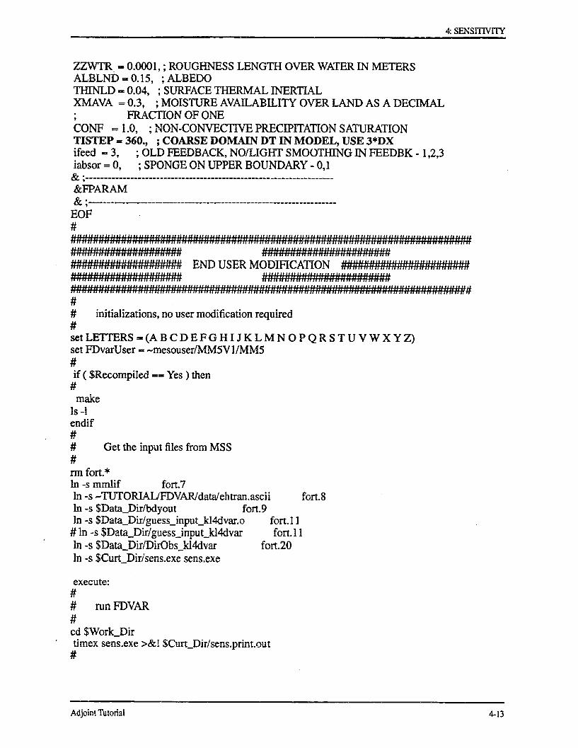
4.4 The job deck of the sensitivity calculation: sens.deck

# QSUB -r SENS # request name# QSUB -q reg #job queue clasr prem econ

QSUB -eo #

4-10 Adjoint Tutorial

4: SENSITIVITY

# QSUB -o sens.out# QSUB -1M 8Mw# QSUB -IT 5000# QSUB

#ja#

# stdout and stderr together# maximum memory

# time limit# no more qsub commands

set echo## ******* 4dvar batch C shell *******

v*v**:(*s**** *******.******

set Data_Dir = -TUTORIAL/dataset Work_Dir = -tmp-sset Curt_Dir = 'pwd'

# set Recompiled = Yesset Recompiled = No

# recompile the code

# type of 4dvar job

set ReStart = False # True -- restart minimization run## .# local namelist values#cat >! $WorkDir/mmlif << EOF&FDPARAMIFVERIGR 0LRG_PRE = 1, ; 0,1 large-scale precipitation

&OPARAM ; <-- MOD'2

YOU CAN REMOVE THE UNWANTED DATA FROM THE FOLLOWING LISTINGAND USE THE DEFAULT VJALUES DEFINED IN SUBROUTINE 'PARAM'.

IFRST = F, ;RESTEARTIXTIMR =720,

LEVIDN = 0,; level of nest for each domainNUMNC = 1, ID of mother domain for each nestIFSAVE = F, ; SAVE DATA FOR RESTART

SAVFRQ =180., ; ... in minutes.IFTAPE = , ; OUTPUT FOR GRIN backend

TAPFRQ 60., ; ... in minutes.IFPRT 1, ; do not change

PRTFRQ = 180., ; Print output frequency in minutesMASCHK = 30, ; MASS CONSERVATION CHECK (minutes)

&LPARAMiactiv= 1,0,0,0,0,0,0,0,0,0, ; in case of restart: was this domain active?

Adjoi1t T r 4-I!

I-------------------------- ------------------------------------------

9

I.

Adjoint Tutorial 4-1!

4: SENSITIVITY

;************* start physics options ****************

IFRAD =0, ;RADIATION COOLING OF ATMOSPHERE - 0, 1, 2RADFRQ 30., :RADIATION FREQUENCY IN MINUTESICUSTB =1, ;STABILITY CHECK FOR CUMULUS PARAM. - 0(no stab. check), 1IEXICE = 0, ;ICE-PHYSICS IN EXPLICIT SCHEME - 0,1IFDRY = 0 ;FAKE-DRY RUN - 0, 1IMVDIF -0, ;MOIST VERTICAL DIFFUSION IN CLOUDS - 0, 1IBMOIST =0, ;BOUNDARY AND INITIAL WATER/ICE SPECIFIED - 0, 1ICOR3D =1, ;3D CORIOLIS FORCE -0, 1IFUPR =0, ;UPPER RADIATIVE BOUNDARY CONDITION - 0, 1

IBOUDY = 3, 2,22,2,2,2,2,2,2, ;BOUNDARY CONDITIONS - 0, 1,2,3,4IBLTYP = 1, 22, 2, 2, 2, 2, 2, 2, 2, ;PBL TYPE - 0, 1, 2IDRY = 0, 0, 0, 0, 0,0, 0, 0, 0,0 ;MOIST OR DRY CASE - 0, 1IMOIST = 1, 1, 1, 1, 1, 1, 1, 1, 1, ;NON-EXPLICIT, EXPLICIT,- 1, 2ICUPA = 2, 1 1, 1, 1, 1, 1, 1, 1, ;NONE,KUO,GRELL,AS - 1,2,3,4ISFFLX = 1,1, 1, 1, 1,, ,1, 1, 1, ;SURFACE FLUXES - 0, 1ITGFLG = 1, 1,, 1, 1, 1, 1, 1, 11,, ;SURFACE TEMPERATURE - 1, 3ISFPAR = 1,1,1,1, 1, 1,1,1, 1, ;SURFACE CHARACTERISTICS - 0, 1ICLOUD = i1; 1,1, 1, 1, 1 1, ,1, ;CLOUD EFFECTS ON RADIATION - 0,1ICDCON - 0, , 0 0,0, 0, 0,0, 0, 0, ;CONSTANT DRAG COEFFICIENTS - 0, 1IFSNOW = 0, 0, 0, 0, 0, 0, 0, 0, 0, ,SNOW COVER EFFECTS - 0, 1IMOIAV 0 0, O, o0,0., 00,0, O,;VARIABLE MOISTURE AVAILABILITY - 0, 1IVMI = 1, 1, 1, 1, 1,1,1,1, 1,;VERTICAL MiXING OF MOMENTUM - 0, 1HYDPRE = 1.,1.,1.,1.,1,1.,1.,1,I,i1.,.;HYDRO EFFECTS OF LIQ WATER- 0., 1.LEVAP = 1, 1, 1,11,, i, , 1,1,,1 ;EVAP OF CLOUD/RAINWATER - <0, 0, >0ISHALLO= 0, 0, 0 , 0 , 0,0, 0,0,0,0;SHALLOW CONVECTION - 0, 1

;***I********* end physics options ****************

;* ************ start nesting options ****************

nestix = 26, 46, 46, 46, 46, 46, 46, 46, 46, 46,; domain size Inestjx = 31, 6, 1, 61, 61, 61, 61, 61, 61, 61,; domain size Jnesti = 1, , 1, 1, 1, 1, 1 1, 1, ,; start location!nestj = 1, , , 1, 1 , 1, 1, I, 1, 1 ,;startlocationJxstnes = 0., 00., 0., O 0., ) 0., 0., 0., 0 ., ; domain initiationxennes =720.,720.,720.,720.,720.,720.,720. ,720.,720.,; domain completionioverw = 0, 0, , 0, 0, 0, 0, 0, 0, 0, ; overwrite domain

;************* end nesting options ******************

&PPARAMTIMAX = 720., ; IN MINUTES. 720=12h, 1440=24h, 2160=36h, 2880=48hZZLND = 0.1, ; ROUGHNESS LENGTH OVER LAND IN METERS

4-12 Adjoint Tutorial ._,.I - I __ -Adjoint Tutorial4-12

4: SENSITIVITY

ZZWTR 0.0001,; ROUGHNESS LENGTH OVER WAIER IN METERSALBLND 0.15, ;ALBEDOTHINLD = 0.04, ; SURFACE THERMAL INERTIALXMAVA = 0.3, ; MOISTURE AVAILABILITY OVER LAND AS A DECIMAL

; FRACTION OF ONECONF =1.0, ; NON-CONVECTIVE PRECIPITATION SATURATIONTISTEP = 360., ; COARSE DOMAIN DT IN MODEL, USE 3*DXifeed - 3, ; OLD FEEDBACK, NO/LIGHT SMOOTHING IN FEEDBK - 1,2,3iabsor = 0, ; SPONGE ON UPPER BOUNDARY - 0,1

&FPARAM

E---- ----------------EOF

iL l1 ifi frI is 11frif15f5 l 1 1 in #I f f f I of AI o11111 l Jlis io f S tso isi of f is to i t oI J 1 iJ 1ul I J[ / * 1 a Jr 11 I TT I J Ia I T I / r ]IAa I I I_ la

2P:2:/:N/.JtJZ::.../:../:..2: END USER MODIFICATION ./f/ /f...;...t ... f15111119111515 1555 55 1115 15 11551555 9515 55 11 1115 551111 1511 5S1 51# 1155 511 11i1 N 01115 5155

.. m u r r m , . r r f ...............,.., .f n. .f.... .,,, ;I ; ift%, l55ll If f! If If I Jl! l 5 fi 1 1 1 51 11 If ii i u is i1] ] t J l 55 I5 1515 !! ] ~ l fl !! ] ff 55 51 15 5! 51 55 51 55 51 55 5 111 5 5 55 !l

I i If l lr Jr II II IfI I Iit 4 IH Wr I ~ ~/ ~IA I Aa Jr J i a11 I I '1 I I I I a I II I! I I I a a I I I i I I I ~ II [I I 1 I I I aaI II I! a a if a If a Ia I I I1- I I IaaIaJ I I II Idr J -l l fAIII

## initializations, no user modification required#setLETTERS-(ABCDEFGHIJKLMNOPQRSTUVWXYZ)set FDvarUser - ~mesouser/MM5Vl/MM5#if ( $Recompiled =- Yes ) then

#make

ls -Iendif## Get the input files from MSS#rm fort.*In -s mmlif fort.7In -s ~TUTORIAUFDVAR/data/ehtran.ascii fort.8In -s $Data_Dir/bdyout fort.9In -s $Data_Dir/guess_input_kI4dvar.o fort. 11

# In -s $Data_Dir/guess_input_kl4dvar fort. 11In -s $DataDir/DirObs_kl4dvar fort.20In -s $Curt_Dir/sens.exe sens.exe

execute:

# run FDVAR#cd $Work_Dirtimex sens.exe >&! $Curt_Dir/sens.print.out

#

Adon Tuora 4-13 - I -IAdjoint Tutorial 4-13

4: SENSITIVITY ~~~~~~i i l l , --- -

The places where users may want to modify are indicated by bold face lines. They are related towhere to read in the input files, the choice of physics options, and the setting of the dimension andtime step, as well as the place to save the output files.

4-1 Adjn Tuora

4-14 Adjoint Tutorial

4: SENSITIVITY- -- - - ---~~~~~~~~~~~~~~~~~~~~~~~~~~~~~~~~~~~~~~~~~~~~~~~~~~~~~~~~~~~~~~~~,

Figure 4.1: (a) The sensitivity of R defined in (4.1) with respect to the initial temperature fieldfield at o = 0.25, 0.55, 0.85 and 0.95.

Adjoin Tutorial 4-154-15Adjoint Tutorial

4: SENSITVITYI_~ I _n _ --- - - -_

4-1 Adon Tutorial - -IAdjoint Tutorial4-16

5: 4D-VAR1 111 , I __~~~~~~~~~~~~~~~~~~~~~~~~~~~~~~~~~~~~~~~~~~~~~~~~~~~~~~~~~~~~I

4D-VARA 1a 3W9t mm m a S- m W me 8 S W e gm Ba W S mm m ot a = ma t

Purpose 5-3

Physics Options in MM5's 4D-VAR System 5-4

Cumulus Parameterizations 5-4PBL Schemes 5-4Explicit Moisture Schemes 5-4Radiation Schemes 5-4

Procedures to run a 4D-VAR experiment 5-5

A few key parameters to be altered for different assimilation experiments: 5-5Input and output files: 5-6Namelists for user-specified options 5-7Script Variables 5-8

Some Common Errors Associated with 4D-VAR Failure 5-9

ATwin 4D-VARExperiment: 5-10

4D-VAR Job Deck 5-1.2

The main 4D-VAR program: mindry.F 5-18

The MM5 forward model subroutine incorporated with the calculation of (cost function)and (forcing terms): mm5dry.F 5-27

The MM5 adjoint model subroutine incorporated with the forcing terms (calculated inmm5dry.F): adjdry.F 5-33

MM5 Adjoint Tutorial $1- -5-1MM5 Adjoint Tutorial

2: FDVARi lj i ..

5-2_c MM Adon Tutorial _5-2 MM5 Adjoint Tutorial

5: 4D-VAR

4D-VAR

W a ont am afml mFm WmB FI S ms tAnWmss a

5.1 Purpose

The 4D-VAR programs seek the "optimal" IC for a user-pre-defined cost function, which mea-sures the misfit of the model prediction to the given observations in the least-square sense. For dif-ferent data-assimilation objectives, the cost function to be minimized will be different. Therefore,unlike using MM5 modeling system where users can run the job without knowing many of thedetails of the model code, the user needs to modify some of the codes in the MM5 4D-VAR sys-tem to find the solution of their own data assimilation problem, due to the difference in observa-tions to be assimilated, the definition and use of weighting and scaling, and possible the penaltyconstraints users may wish to add. In this section, we will describe the 4D-VAR system in detailwith the hope that users can not only run the standard 4DVAR experiment, but also run their own4DVAR experiment with ease.

The job deck, main program, and a few subroutines which may need user interactions for carryingout 4D-VAR experiment are placed in the subdirectory main minimization:

-fdvar/Tutorial_97/main_minimization/fdvar.deck-fdvar/Tutorial_97/main_minimization/mindry.F-fdvar/Tutorial_97/main_minimization/mairnmm5dry.F-fdvar/Tutorial_97/main_minimization/main/adjdry.F-fdvar/Tutorial_97/main_minimization/main/objfun.F-fdvar/Tutorial_97/main_minimization/main/gradcl.F

The subroutine mindry.F is the main driver to carry out the minimization procedure (see Fig. 1 inZou et al., 1997), mm5dry.F and adjdry.F are the MM5 and MM5 adjoint model incorporatedwith the calculation of the cost function and proper forcing terms for the gradient calculation ofthe cost function (see Fig. 2 in Zou et al., 1997), the subroutine objfun.F calls the forward modelmm5dry.F from the minimization routines in which the control variables is a one-dimensionalarray, and gradcl.F calls the adjdry.F to get the scaled gradient value during the minimization process. Before we move on to explain how to run a 4D-VAR experiment, we first mention the phys-ics options available in the MM5 adjoint model system:

MM5 Adon Tuora 5-3,II _ ,_MM5 Adjoint Tutorial 5-3

5: 4D-VAR

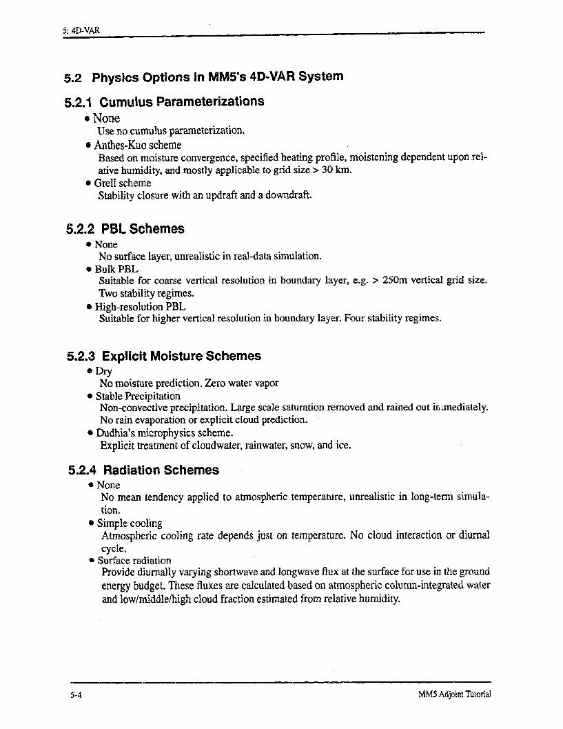
5.2 Physics Options in MM5's 4D-VAR System

5.2.1 Cumulus Parameterizationse None

Use no cumulus parameterization.* Anthes-Kuo scheme

Based on moisture convergence, specified heating profile, moistening dependent upon rel-ative humidity, and mostly applicable to grid size > 30 km.

* Grell schemeStability closure with an updraft and a downdraft.

5.2.2 PBL Schemes* None

No surface layer, unrealistic in real-data simulation.Bulk PBLSuitable for coarse vertical resolution in boundary layer, e.g. > 250m vertical grid size.Two stability regimes.

* High-resolution PBLSuitable for higher vertical resolution in boundary layer. Four stability regimes.

5.2.3 Explicit Moisture Schemes*Dry

No moisture prediction. Zero water vapor* Stable Precipitation

Non-convective precipitation. Large scale saturation removed and rained out inimmediately.No rain evaporation or explicit cloud prediction.

* Dudhia's microphysics scheme.Explicit treatment of cloudwater, rainwater, snow, and ice.

5.2.4 Radiation Schemes* None

No mean tendency applied to atmospheric temperature, unrealistic in long-term simula-tion.

* Simple coolingAtmospheric cooling rate depends just on temperature. No cloud interaction or diurnalcycle.

e Surface radiationProvide diurnally varying shortwave and longwave flux at the surface for use in the groundenergy budget. These fluxes are calculated based on atmospheric column-integrated waterand low/middle/high cloud fraction estimated from relative humidity.

-4 MM5i . -A djoin -- Tut oria

M.M5 Adjoint Tutorial5-4

5: 4D-VARI ---- I ---~~~~~~~~~~~~~~~~~~~~~

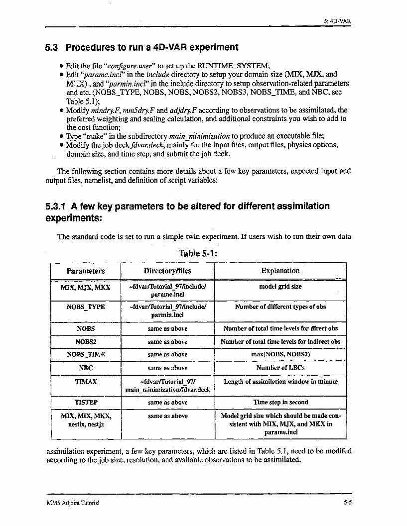
5.3 Procedures to run a 4D-VAR experiment

* Edit the file "configure.user" to set up the RUNTIME_SYSTEM;E Edit "parame.incr' in the include directory to setup your domain size (MIX, MJX, andMI-X) , and "parmin.incrl in the include directory to setup observation-related parametersand etc. (NOBSTYPE, NOBS, NOBS, NOBS2, NOBS3, NOBSTIME, and NBC, seeTable 5.1);

* Modify mindry.F, rnm5dry.F and adjdry.F according to observations to be assimilated, thepreferred weighting and scaling calculation, and additional constraints you wish to add tothe cost function;

* Type "make" in the subdirectory mainminimization to produce an executable file;* Modify the job deckfdvardeck, mainly for the input files, output files, physics options,

domain size, and time step, and submit the job deck.

The following section contains more details about a few key parameters, expected input andoutput files, namelist, and definition of script variables:

5.3.1 A few key parameters to be altered for different assimilationexperiments:

The standard code is set to run a simple twin experiment. If users wish to run their own data

Table 5-1:

Parameters Directory/files Explanation

MIX, MX, MKX -fdvar/Intorial 97fnclude/ model grid sizeparameJncl

NOBS TYPE -fdvar/atorial 97include/ Number of different types of obsparmin.incl

NOBS same as above Number of total time levels for direct obs

NOBS2 same as above Number of total time levels for indirect obs

NOBS Tlla same as above l max(NOBS, NOBS2)

NBC same es above Number of LBCs

TIMAX -fdvar/utorial 7/ Length of assimilation window in minutemainrminimizationffdvardeck

TiSTEP same as above Time step in second

MIX, MIX, MKX, same as above Model grid size which should be made con-nestix, nestjx sistent with MIX, MJX, and MKX in

parame.incli ~ .. . - -

assimilation experiment, a few key parameters, which are listed in Table 5.1, need to be modifedaccording to the job size, resolution, and available observations to be assimilated.

MM5-- AdjointI- Tutorial 5-5

5-5M-M,5 Adjoint Tutorial

5: 4D-VAR

5.3.2 Input and output files:

Input files:

1) Standard MM5 initial file and boundary file:

* InBdy = MM5.BC (standard MM5 LBC input file)* InMM = MM5.IC (standard MM5 IC file)

2) Observations

* Direct and/or indirect observations

3) Restart files for a restart minimization

* Restart.file: fort.50 (minimization information), ISOL ("optimal" initial perturba-tion), ICDIR (search direction), ICGRAD (current gradient), IOGRAD (previous gradient)

Output files:

1) ICs at every iteration: ITER.tar

2) Values of the gradient at every iteration: GRAD.tar

3) A print file print.tar containing fdvar.print.out mmlif fdvar.deck acct

4) Restart file: fort.50 (minimization information), ISOL ("optimal" initial perturbation),ICDIR (search direction), ICGRAD (current gradient), IOGRAD (previous gradient)

In-job files:

Weighting, scaling, initial guess, basic states, forcing terms, current and previous gradi-ents, and search direction.

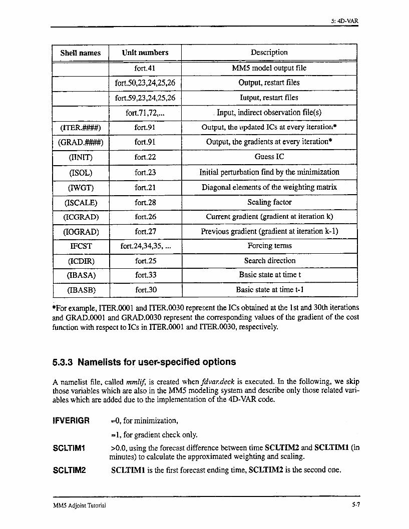
In 4D-VAR, different input and output data are written to separate files, and most files areaccessed by specified Fortran unit numbers, which are assigned as follows:

Table 5.2 Shell names, Fortran unit numbers, MSS names and their usages:

5 -6 M M A d j o i nt_ T u t o r i a l , _,_ _ , ,

Shell names Unit numbers Description

mmlif fort.7 Input, namelist file

ehtran fort.8 Input, emissivity file

InBdy fort.9 Input, boundary files created by program INTERP

InMM fort. 1 Input, initial files created by program INTERP

DirObs fort.20 Input, direct observations

5-6 MM5 Adjoint Tutorial

5: 4DVARI -.

Shell names Unit numbers Description

fort.41 MM5 model output file

fort.50,23,24,25,26 Output, restart files

fort.59,23,24,25,26 lutput, restart files

fort.71,72,... Input, indirect observation file(s)

(ITER.###) fort.91 Output, the updated ICs at every iteration*

(GRAD.####) fort.91 Output, the gradients at every iteration*

(INIT) fort.22 Guess IC

(ISOL) fort.23 Initial perturbation find by the minimization

(IWGT) fort.21 Diagonal elements of the weighting matrix

(ISCALE) fort.28 Scaling factor

(ICGRAD) fort.26 Current gradient (gradient at iteration k)

(IOGRAD) fort.27 Pevious gradient (gradient at iteration k-1)

IFCST fort.24,34,35,... Forcing terms

(ICDIR) fort.25 Search direction

(IBASA) fort.33 Basic state at time t

(IBASB) fort.30 Basic state at time t-1

*For example, ITER.0001 and ITER.0030 represent the ICs obtained at the 1st and 30th iterationsand GRAD.0001 and GRAD.0030 represent the corresponding values of the gradient of the costfunction with respect to ICs in ITER.0001 and ITER.0030, respectively.

5.3.3 Namelists for user-specified options

A namelist file, called mmlif, is created when fdvar.deck is executed. In the following, we skipthose variables which are also in the MM5 modeling system and describe only those related vari-ables which are added due to the implementation of the 4D-VAR code.

IFVERIGR

SCLTIM1

SCLTIM2

=0, for minimization,

= 1, for gradient check only.

>0.0, using the forecast difference between time SCLTIM2 and SCLTIM1 (inminutes) to calculate the approximated weighting and scaling.

SCLTIM1 is the first forecast ending time, SCLTIM2 is the second one.

MM Adjin Tuora 5.7 I ----- -

MMt5 Adjoint. Tutorial 5-7

5: 4D-VAR- _

IRESTART -TRUE, if it is a restart run,

-FALSE, if it starts from zeroth iteration.

MSSPATH =MSS path to save the restart files.

OBSTIME >0, Direct observation is to be assimilated, put the time in minutes

<0, No direct observation

OBSTIME1 same as OBSTIME except for the first indirect observation.

OBSTIME2 same as OBSTIME except for the second indirect observation.

ITREND =Maximum iteration number.

MSSINTV -Iteration interval to save the minimization restart files.

NOT_UU =TRUE, Zero out u weighting, i.e. not assimilate direct observation u,

=FALSE, assimilate u.

NOT_VV -TRUE, Zero out v weighting, i.e. do not assimilate direct observation v,

-FALSE, assimilate v.

NOTT -TRUE, Zero out T weighting, i.e. do not assimilate direct observation T,

=FALSE, assimilate T.

NOT_QQ =TRUE, Zero out qv weighting, i.e. do not assimilate direct observation qv,

=FALSE, assimilate qv.

NOT_PP =TRUE, Zero out p' weighting, i.e. do not assimilate direct observation p',

=FALSE, assimilate p'.

NOT_WW =TRUE, Zero out w weighting, i.e., do not assimilate direct observation w,

=FALSE, assimilate w.

NCEP_WEIGHT =0, using the difference between two direct observations to calculate approxi-mated weighting and scaling,

=1, using NCEP's statistic error to calculate weighting and scaling.

ICOEFFNT -1, user specifies values of the weighting for indirect observations,

=0, model calculates the weighting factors for indirect observations which bal-ance each term in the cost function

LRGPRE -1, include the large-scale precipitation,

=0, exclude the large-scale precipitation

5.3.4 Script Variables

In this subsection, we briefly describe the script variables used in thefdvar.deck.

5l M A i Ttra

MM5 Adjoint 'I torial5-8

5: 4D-VAR

NCPUS number of processors (set NCPUS=1, 4D-VAR codes are not multitasked).

ExpName experiment name used in setting MSS pathname.

InName input MSS pathname.

InRst MSS name(s) of model restart files.

RetPd mass store retention period (days).

recompiled =yes, recompile the FDVAR code;

=no, expect an existing executable.

CaseName MSS pathname for this run.

OutMM MSS name for output

RESTART =FALSE: start model run at zero iteration.

=TRUE: restart model run.

InBdy MSS name of boundary file.

InMM MSS name(s) of model input files.

DirObs MSS name(s) of direct observation file.

5.4 Some Common Errors Associated with 4D-VAR Failure

When a 4D-VAR job is completed, always check for at least the following:

The "STOP 99999" print statement indicates that 4D-VAR WAS completed successfully.

When running a Cray job, check to make sure that the mswrite commands were all completed by

the shell, and do a msls to check that all the files were written to the pathnames you expected.

Check the top of "fdvar.print.out" file to see if the physics options are correctly specified.

If a 4D-VAR job has failed, check these too.

"Read past end-of-file": This is usually followed by a fortran unit number. Check this unit numberwith Table 5.2 to find out which file the read error is related in the 4D-VAR problem. Check all the

msread statements in the print out to make sure that the file was read properly from the mass stor-age. Also check to make sure that the file size is non-zero. Double-check experiment names and

MSS pathnames.

"CPU limit exceeded": Increase the amount of time requested in the QSUB statements when run-ning the job on a Cray.

"Not enough space": Increase the amount of memory requested in the QSUB statements when

1 . . . . .I -.


5: 4D-VAR- I I I I I I I I --- · L _

running on a Cray.

"'Unrecognized namelist variable"': This usually means there are typoes in the namelist.

Unmatched physics option: for instance, the following should appear in the output:STOP SEE ERRORS IN PRINT-OUT

Uncompiled options:STOP SEE ERRORS IN PRINT-OUT

If one browses through one's output, one may find things like:ERROR: IFRAD=2, OPTION NOT COMPILED

which tells the user the option you choose has not been compiled.

When restarting a job, do not re-compile the code. If you do, do not change anything in the config-ure.user file.

If the job stopped and there was a long list of "CFL>1 ...", it can mean that the time step (TISTEPin namelist) is too big or there are other hidden bugs.

5.5 A Twin 4D-VAR Experiment:

In order to make a "cheap" (computationally) and "clean" (knowing the answer) test of the MM54D-VAR system, we designed a standard twin 4D-VAR experiment in which "observations" aregenerated by the assimilation model itself. Most of the components in the 4D-VAR experimentcould be well tested in such an identical-twin-experiments 4D-VAR framework. The advantage ofconducting the twin experiments is that the true solution is known exactly, and the minimum valueof J is zero. It thus allows users to test the accuracy of the code, to examine the performance andcapability of the minimization procedure, to assess the speed of convergence and to estimate thecomputational expenses of such an assimilation.

The 4D-VAR identical twin experiment is initialized at 0000 UTC 13 March 1993. The initialcondition was based on the NCEP global analysis, following an objective analyses of rawinsondeand surface observations, which were also carried out for the other time levels between 0000 UTC13 March to 0000 UTC 14 March 1993 at 12-h interval. The 12-h LBCs were obtained by linearinterpolation of the analyses. These IC and LBCs were done at 120-km resolution, with a grid sizeof 26x31. There are 10 evenly-spaced Y levels in the vertical on both horizontal grids.

The cost function is defined as

3.bs obs. (5.1)

J = E (X(tr)-X(tr) ) W(X(tr)-x(tr) .r=O

obswhere x (tr) , r=0,1,2, and 3 is the MM5 analysis at t = to (0000 UTC 13 March 1993, thetrue IC), and the 1-h, 2-h and 3-h model prediction starting from the "true" IC .

Before a minimization procedure is carried out, a gradient check is suggested to make sure that

.1 M M __ A T tr


5: 4D-VAR

the values of the cost function and the gradient of the cost function with respect to the IC is cor-rectly calculated. Results of such a check for the above twin experiment are shown in Table 5.3 asfollows (see (3.17) in Zou et al. 1997).

Table 5-2:

10-4 0. 1229677822E+01

10-5 0.1062315239E+01

-6 0.1000022605E+0110

1-7 0.1000003295E+01

-8 0.1000000662E+01

-109 0.1000000025E+01

-10 0. 1000013606E+0110

-11 0.1000161181E+01

10-12 0.1001126464E+01

l-13 |0.1011717534E+01

in which the first column shows the values of a which controls the magnitude of the initial pertur-bations, the second and the third columns show the values of 4y(a) with and without includingthe large-scale precipitation, respectively.

The minimization starts from a guess IC which is the analysis at t = to . We find that the valuesof both the cost function and the norm of the gradient with respect to the IC decreased 5 and 3orders of magnitude respectively (Fig. 5.1) in 20 iterations. In order to examine how the differ-ence fields between the updated IC and the true IC and their subsequent forecasts are modified inthe process of minimization, we also plotted the errors in the 300-mb wind fields (Fig. 5.2) andtemperature fields at 0=0.95 (Fig. 5.3) at the 0th, 2nd, and 5th iteration, respectively. We foundthat most errors are corrected during the first few iterations.

5.6 4D-VAR Job Deck

# QSUB -r FDVAR # request name

5-11MM5 Adjoint Tutorial

g -- I -- I

5: 4D-VAR__. i! i

# QSUB -q reg# QSUB -eo# QSUB -o fdvar.out# QSUB -IM 8Mw# QSUB -IT 5000# QSUB#Ja

#set echo

# *88*****

# job queue class prem reg econ## stdout and stderr together# maximum memory# time limit

# no more qsub commands

cd $TMPDIR#batchname fdvarbatch.out

## how many CRAY CPUs to use to run the model, set to 1 if not multitasking#setenv NCPUS 1

set ExpName = TUTORIALset InName = /FDVAR/TUTORIALset InRst = $ExpName/RESTARTset RetPd = 999##set Recompiled - Yesset Recompiled = No

set CaseName = TEST

# recompile the code

# MSS directory for output file#set OutMM = ${ExpName}/${CaseName}## type of 4dvar job#set RESTART = False # True -- restart minimization run

# Give the MSS file names of input data##.. Lateral boundary input file:set InBdy = ${InName}/MM5.BC

#.. Standard MM5 input file:set InMM = ${InName}/MM5.IC

5-12,,,~~~~~~~~~~~~~~~~~~~~~~~~~~~~~~~~~~ i A T

4dvar~ batch C shell

5-12 MM5S Adjoint Tutorial

5: 4D-VAR_- I K. -- --I

#.. Direct observed analysis data file (direct access file):set DirObs = ${InName})DIRECT_OBS

if( $RESTART = True ) then# . Get the files for restart:

msread fort.59 ${ExpName)/RESTART/Restart.filemsread fort.23 ${ExpName)/RESTART/ISOLmsread fort.25 ${ExpName)/RESTART/ICDIRmsread fort.26 ${ExpName}/RESTART/ICGRADmsread fort27 ${ExpName}/RESTART/IOGRAD

endif## local namelist values#cat >! mmlif << EOF&FDPARAM

IFVERIGR = 0, ; 1 -> GRADIENT CHECK ONLY, 0 -> MINIMIZATION

; if SCLTIM2 > 0.0, using forecasts at SCLTIM 1 and SCLTIM2 to calculate; the weighting and scaling:SCLTIM1 = 0.0, ; in minutesSCLTIM2 = 0.0, ; in minutes

RESTART = .$RESTART., ; .T. -> restart runMSSPATH - '${InRst}', ;MSS path directory for restart files9

; The model time in minute when the observations are available; 1 2 3 4 5 6 7 8 9 10 11 12 13

OBSTIME = 0.0, 60.,120.,180.,-9.9,-9.9,-9.9,-9.9,-9.9,-9.9,-9999,-9.9,OBSTIME2 = -9.9,-9.9,-9.9,-9.9,-9.9,-9 .9,-9.9,-99 9.9,OBSTIME3 = -9.9,-9.9,-9.9,-9.9,-9.9,-9.9,-99-9.9,-9.9,-9.999,-9.9,-9.9,

ITREND = 5, ; ending iterationsMSS INTV= 5, ; interval

; Set .T. to select the variables which are not assimilated:NOT UU = .F.,NOTW = .F.,NOTTT = F.,NOTQQ = F.,

NOT PP =.,NOT WW = F.,NOT TG = .T,NCEP WEIGHT = 0, ; 0 maximum obs diff, 1 NCEP weightICOEFFNT = 1, ; 1 user-specified weighting for indirect obs, 0 balance weight

MM Adjin Tuora 5-13- --5-13MM5 Adjoint Tutorial

5: 4D-VARill-_ __

LRGPRE = 1, ; 0,1 large-scale precipitation

&OPARAM ; <-- MOD2

; YOU CAN REMOVE THE UNWANTED DATA FROM THE FOLLOWING LISTING; AND USE THE DEFAULT VALUES DEFINED IN SUBROUTINE 'PARAM'.

IFREST F, ;RESTARTIXTIMR =720,

LEVIDN 0, ; level of nest for each domainNUMNC 1,; ID of mother domain for each nestIFSAVE = F, ; SAVE DATA FOR RESTART

SAVFRQ 180, ; ... in minutes.IFTAPE - 1, ; OUTPUT FOR GRIN backend

TAPFRQ 60., ; ... in minutes.IFPRT = 1, ; do not changePRTFRQ - 180., ; Print output frequency in minutesMASCHK = 30, ; MASS CONSERVATION CHECK (minutes)

&LPARAMiactiv=l,0,000,0,0,0,0,0,,,; in case of restart: was this domain active?

;************* start physics options ***************

IFRAD - 0, RADIATION COOLING OF ATMOSPHERE - 0, 1, 2RADFRQ -30., :RADIATION FREQUENCY IN MINWTESICUSTB - 1, ;STABILITY CHECK FOR CUMUIUS PARAM. - 0(no stab. check), 1IEXICE =0, ;ICE-PHYSICS IN EXPLICIT SCHE - 0, 1IFDRY = 0, ;FAKE-DRY RUN - 0, IIMVDIF =0, ;MOIST VERTICAL DIFFUSION IN CLOUDS- 0, 1IBMOIST -0, ;BOUNDARY AND INITIAL WATER/ICE SPECIFIED- 0, 1ICOR3D =1, ;3D COPIOLIS FORCE -0, 1IFUPR = 0, ;UPPER RADIATIVE BOUNDARY CONDITION - 0, 1

IBOUDY = 3, 2, 2, 2, . 2,2, 2, 2, 2;BOUNDARY CONDIONS - 0, 1, 2, 3, 4IBLTYP= 1, 2,2, 2,2,2,2,2, 2, ,;PBL TYPE- 0, 1,2IDRY =0, 0,0, 0, 0,0,0, 0,0, 0, ;MOIST OR DRY CASE - 0, 1IMOIST= 1 1, 1, , 1, 1, 1, , 1, 1, ;NON-EXPLICIT, EXPLICIT, - 1, 2ICUPA = 2, 1, 1, 1, , 1, ,1 , 1,, ;NONE,KUO,GRELL,AS - 12,3,4ISFFLX= 1,1, 1, 1, 1, 1, 1,1, ; 1 SURFACE FLUXES - 0, 1ITGFLG = 1, 11,1, ,1,, 1, 1, 1, 1,;SURFACE TEMPERATURE - 1, 3ISFPAR = 1, 1, 1, I, 1, 1, 1, 1, i, ;SURFACE CHARACTERISTICS - 0, 1ICLOUD = 1, 1, 1, , 1, 1, ,1, 1, , ;CLOUD EFFECTS ON RADIATION -0, IICDCON = 0,0, 0, 0, 0, 0, ,0 0, 0, 0;CONSTANT DRAG COEFFICIENTS - 0. 1IFSNOW =0 00, 0, 0, 0, 0, 0.0,0, ;SNOW COVER EFFECTS - 0, 1IMOIAV = 0, 0, 0, 0, 0, 0, 0,0, ,0 ;VARIABLE MOISTURE AVAILABILITY - 0, 1

5 -4 M M Adj in Tutorialg - - I - ,5-14 MM5 Adjoint Tujtorial:

5: 4D-VAR

IVMIXM = 1, 1, 1, 1,1, 1, ,1 1, 1,1, ;VERTICAL MIXING OF MOMENTUM - 0, 1HYDPRE= 1.,1., 1., 1., 1., 1., 1., 1., 1.,;HYDRO EFFECTS OF LIQ WATER - 0., 1.IEVAP =1 1, ,1, 1, 1, 1, 1,1, 1, ;EVAP OF CLOUD/RAINWATER - <0, 0, >0ISHALLO= ,0, 0, 0, 0, 0,,0 0, 0, 0,;SHALLOW CONVECTION - 0, 1

9;************* end physics options ******************

************* start nesting options ****************

nestix = 26, 46, 46, 46, 46, 46, 46, 46, 46, 46,; domain size Inestjx=31, 61, 61, 61, 61, 61, 61, 61, 61, 61,; domain size Jnesti = 1, 1, 1, 1, 1, 1, 1, 1, , 1, ;start location Inestj = 1, 1, 1, 1, 1, 1, 1, 1, 1, 1,;startlocationJxstnes = 0., 0., 0., 0., 0., 0., 0., 0., 0., 0.,; domain initiationxennes =1440.,720.,720.,720.,720.,720.,720.,720.,720.,720.,; domain completionioverw = 0, 0, 0, 0, 0, 0, 0, 0, 0, 0,; overwrite domain

;.************* end nesting options ******************

&PPARAMTIMAX = 180., ; IN MINUTES. 720=12h, 1440=24h, 2160=36h, 2880=48hZZLND = 0.1, ; ROUGHNESS LENGTH OVER LAND IN METERSZZWTR = 0.0001,; ROUGHNESS LENGTH OVER WATER IN METERSALBLND = 0.15, ; ALBEDOTIIINLD = 0.04, ; SURFACE THERMAL INERTIALXMAVA = 0.3, ; MOISTURE AVAILABILITY OVER LAND AS A DECIMAL

FRACTION OF ONECONF =1.0, ; NON-CONVECTIVE PRECIPITATION SATURATIONTISTEP = 360, ; COARSE DOMAIN DT IN MODEL, USE 3*DXifeed =- 3, ; OLD FEEDBACK, NO/LIGHT SMOOTHING IN FEEDBK - 1,2,3iabsor = 0, ; SPONGE ON UPPER BOUNDARY - 0,1

&FPARAM

EOF

1A AI SAAaAA i A is as , 1A to if of ,I S as off to is of di asl 111 Ai AA is Al 1 as is is 1, 1 9 S. . of as ON so as of it at Ai of rr f A 11Is 1 1Is ilt. It it 1so111tl RZ s1 !

.. K..........H5............. END USER MODIFICATION #####I###i,' ##.####111f15 1 o i II i o 11I1 l! 11 1 51 11 Is II It 1fI s 1 11 if 1 1[ i5J! IttoI t of I s J It It if it If 11 If 1 1 5I I s 11 I f so i s i fi I5 . If 1 It II S1 5 i if to if I 5 5 Ito

# initializations, no user modification requited

setLETTERS=(ABCDEFGHIJKLMNOPQRSTUVWXYZ)set FDvarUser = ~mesouser/MM5V1/MM5

MM Adon Tuora 5-15, - --- ,- -5-15MM5 Adjoint Tutorial

5: 4D-VAR

#if ( $Recompiled -= Yes ) thenmake

mswrite -t 1000 fdvar.exe $OutMM/fdvar.exels -I

elsemsread fdvar.exe $OutMMlfdvar.exechmod +x fdvar.exe

endif## Get the input files from MSS#if( ! -e InBdy ) msread InBdy $InBdyif( ! -e riMM ) msread InMM $TnMMif( ! -e DirObs ) msread DirObs $DirObs

## set up fortran input files for 4DVAR#rm fort.*In -s mmlif fort.7In -s ${FDvarUser}/ehtran fort.8In -s InBdy fort.9In -s InMM fort. 11In -s DirObs fort.20

#ln -s InDirPW fort.71#ln -s InDirRN fort.77#execute:

## run FDVAR#datefdvar.exe >&! fdvar.print.out

ja -st >! acctcat acct >> fdvar.print.outcat fdvar.print.out#tar -cvf GRAD.tar GRAD.*

mswrite -t 900 GRAD.tar $OutMM/GRAD.tar#

tar -cvf ITER.tar ITER.* LAST.*mswrite -t 900 ITER.tar $OutMM/ITER.tar

tar -cvf print.tar fdvar.print.out mmlif fdvar.deck acctmswrite -t 900 print.tar $OutMM/print.tar

5 - 1 M M A d o n T u t r i a5-16 MM5 Adjoint Tutorial

5: 4D-VAR

rm GRAD.tar ITER.tar print.tar

MM Adjin Tutria 5-175-17MM5 Adjoint Tutorial

5: 4D-VAR

5.7 The main 4D-VAR program: mindry.F

PROGRAM MINDRYSAVE

CcccccccccccccccCCCCCCCCCCC CCCCCCCCCCCCCCCCCCCCCCCCCCCCC CCCCCCCCCCCCCCCC CC L-BFGS minimization with a nonhydrostatic version of mm5 CC CCCCCCCCCCCCCCCCCCCCCCCCCCCCCCCCCCCCCCCCCCCCCCCCCCCCCCCccccccccccccccc# include <parame.incl># include <pannin.incl># include <param2.inc!># include <param3.incl># include <addrO.incl># include <various.incl># include <dusolve l.incl># include <variousn.incl># include <point3d.incl># include <point2d.incl># include <pointbcincl># include <nonhyd.incl># include <nonhydb.incl># include bcontrol.incl># include <minim.inci>C

DIMENSION AUA (MIX,MJX,MKX),AVA (MIX,MJX,MKX),ATA(MIXMX,MKX ),AQVA(MIXMJX,MKX),APPA(MIX,MJX,MKX),AWA(MIXMJX,KXP NH),AQCA(MIXM ,MJXM ,MKXM ),AQRA (MXM ,MJXM ,MKXM ),AQIA(MIX!CMJXCMKXIC),AQNIA(MIXIC,MJXIC,MKXIC),ATGA(MIX,MJX)

DIMENSION IFCST(NOBSTYPE)COMMON /LRG-PRECIPITATION/L G_PRE

CCOMMON /SCRTCH/XSBB(NDIMSEB),XSS(NDIMS),

- ZZZ(NSCRTCH-NDIMSBB-NDIMS)CC L-BFGS

LOGICAL FINISHC MM5

INTEGER IEXEC(MNAXNES)INTEGER TRIMLEN, LEN_MSSPATH

C OUTPUT FILENAMECHARACTER FILENAIVIE*9

# include <obsdata.incl>CC^ASAAAAAAAAAAAhAAA AAF^AAAAAAAAA AAAAAAAAAAAA AAAA

CICOEFFNT-INCEPWEIGHTO0LRG_PREsIMSSPATH - 'TMPDIRECTORYTOSAVEYOURRUNTIME _FE/'READ (7,FDPARAM)PRINT FDPARAM

CLENMSSPAAH TRIMLEN(MSSPATH)IF(MSSPATH(LENMSSPATHI:LENMSSPATH) .NE. '/') TEN

LEN MSSPATH - LEN_MSSPATH + 1MSSPATH(LEN_MSSPATHT:EN_MSSPATH) - '

ENDIFCC-- INITIALZE TO ZEROC

DO I N=I,MAXNES

5-1 MM Adjin Tutorial ~ --NMM5 Adjoint Tutorial5-18

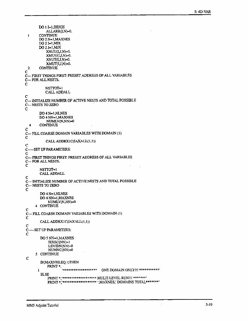
5: 4D-VAR

DOI I,IHUGEALLARR(I,N)-O.

1 CONTINUEDO2 N- 1,MAXNESDO 2 I-1,MIXDO 2 J-1,MX

XNUU(IJ,N)=0.XMfJU(I,J,N)c0.XNUT,JN)-0.XMUT(IJN)-O.

2 CONTINUECC--- FIRST THINGS FIRST: PRESET ADDRESS OF ALL VARIABLESC--- FOR ALL NESTS.C

NSTIOT 1CALL ADDALL

CC--- INITALIZE NUMBER OF ACTIVE NESTS AND TOTAL POSSIBLEC-- NES TO ZEROC

DO 4 N-INLNESDO 4 NN-1,MAXNES

NUMLV(N,NN)-04 CONTINUE

CC--- FILL COARSE DOMAIN VARIABLES WITH DOMAIN (1)C

CALL ADDRX C(IAXALL1,I ))CC-SET UP PARAMETERS:CC- FIRST THINGS FIRST: PRESET ADDRESS OF ALL VARIABLESC-- FOR ALL NESTS.C

NSTTOT-1CALL ADDALL

CC--- INITIALIZE NUMBER OF ACTIVE NESTS AND TOTAL POSSIBLEC-- NESTS TO ZEROC

DO 4 N-1,NLNESDO 4 NN-1,MAXNES

NUMLV(N4NN)0O4 CONTINUE


CALL ADDRX C(IAXALL( I1))CC---SET UP PARA-METERS:C

DO 5 NN-1,MAXNESrIXEC(NN)=iLEVIDN(NN)O0NUMNC(NN)-O

5 CONTINUEC

IF(MAXNES.EQ. 1)TIENPRINT*,

1 '************* ONE DOMAIN ONLY!!! ***********'ELSE

PRINT $ '***-******e**** MULTI LEVEL RUN!!! ******'

PRINT *'***** *AXNES*,**' DOMAAIN*S ! TOTAL*******'

MM Adon Tuoia 5-19,

- -~~C L5-19MM5 Adjoint Tutorial

5: 4D-VAR

ENDIFCC--- READ IN PARAMETERS AND NAMELISTSC

CALL PARAM(IEXEC)CC READ IN SUBSTRATE TEMPERATURE:C

READ(9) TMNCALL SKIFF (9, IERR)

CC READ IN THE BOUNDARY CONDITIONS:C

CALL BDYIN(9,TBDYBE,BDYTIM,ILJL,IBMOIST)CC obtained values of UEBC,UEBCT......CC-- READ IN THE COARSE GRID INITIAL CONDITIONSC

CALL MRDINIT(I 1, IL, JL, 0)C A A A A

C I I I -- 1 READ HEADER ON DATA SETC I ----.--- I SIZE OF THIS DOMAINC ---------... - UNIT OF INITIAL CONDITION FILECC obtained values of UA,VA......WAC

CALL MINO(IEXEC,ILJL)CC obtained values of 2-D fields (not variabC

NBAS - NINT(TMAX*60ODT)+lDTIN-DTEXTIME 0.DTINC -0.

c Total time steps in assimilation wind TIMAX (in minute)NBAS - NINTTIMAX*60DT)+ IPRINT *,' - THE NUMBER OF BASIC STATES NBAS -'NBAS,' -MAXSTP-NBAS-1

c sequential data filesCC----Define observation file(s) unit.CC---IOBS(l)for direct observationC---IOBS(2)......for other indirect observations.C

IOBS(1)20CC----Define weighting unit.C

IWGT-21CC----Define guessfield's unit.C

IINIT-22CC----Define perturbation solution's unit.C

ISOL-23C

5-2 MM5 Adon Ttra


5: 4D-VAR

C----Define units for gradients and search Direction.C

ICDIR-25ICGRAD-26IOGRAD-27

CC----Define scaling unit.C

ISCALE-28c direct access data filesCC----Define units for basic state file(s).C

IBASB=30IBASA- 33

CC--- Define unitsfor theforcing terms.C

IFCST( 1)24NDIM2D>MIX*MJXCALL ASTART(IBASB, NDIMS)CALL ASTART(IBASA, NDIMS)CALL ASTART(IFCST(1), NDIMSS)CALL ASTART(IFCST(2),NDIMSr)CALL ASTART(IFCST(3)NDIM2D)

LENGTH_OF_SOUNDIMIX*MJX*(7*MKX+1 )CALL ASTART(91, LENGTH_OFSOUND)

c Basic state update frequencyDO IT-I,NBAS

IBSTEP(rIT)IT-ENDDO

c Time levels of obs.c direct OBS

DO 2221 IT-I,NOBSITSTEP(1,IT) - NINT(OBSTIME(IT)*60yJDUIN)

2221 CONTINUE

Cc-- Calculate weighting and scaling from either two given analyses or two forecastsc

CALL TRANSF( 1,XSBB,NDIMSBB, UA, VA, TA, QVAPPA, WA,MIX,MJX,MKX,

-QCA, QRA,MIXM, MJXM, MKXM, IEXMS,- QIA,QNIA,MIXICJXI CX KXIC,IICE)

cCALL APUT(IINIT, I,NDIMSBB,XSBB)

CIF (SCLTIM2.L.E.O.) THEN

C.. use 2 time-level all-variable direct observations (IOBS(1)) toc calculate dhe scaling factorCC----Get Direct Obsevation(s).C

print*,'NOBS-',NOBS,' 'INDIMOBSS-',NDIMOBSSCALL AGET(IOBS(!), 1,NDIMOBSS,XSBB)CALL AGET(IOBS( 1 ),(NOBS- 1)*NDIMOBSS+ ,)NDIMOBSSXSS)

CELSE

C .. use the SCLTIM2 minutes model forecasts to calculate the weighting and scale

MM5- Adon Tuoia 5-21--- r -


5: 4D-VAR

LENGTHI- NINT((SCLTIM I*60.)/DT)LENGTH2- NINT((SCLTIM2*60.YDT)IF (LENGTH.IEQ.0) THEN

CALL AGET(IINIT, ,NDIMSBB,XSBB)ELSE

CALL NLMOD(LENGTHI,DTIN)CALL TRANSF( I,XSBB ,NDIMSBB, UA, VA, TA, QVAPPA, WA,

- MIX,MJX,MKX,QCA, QRA,MDCM, MJXM, MKXM, IEXMS,

- QIA,QNIA,MIXICMJXICIMKXIC,IICE)ENDIF

LENGTH2- NINT((SCLTIM2*60.)/DT)CALL NLMOD(LENGTH2,D)TN)CALL TRANSF( 1,XSS ,NDIMSS, UA, VA, TA, QVA,PPA, WA,

- MIX,JX,MKX,QCA, QRA,MIXM, MJXM, MKXM, IEXMS,

- QIA,QNIA,MIXIC,MJXIC,MKXIC,ICE)ENDIF

CC (1) scaling factorc Maximum difference (Max(abs(u I-u2)))

CALL MAXDIFF(XSBB,NDIMSBB,XSS,NDLMS,- UMAX,VMAX,TMAX,QVMAXPPMAX,WMAX,- M,MJX,MKX,- QCMAX, QRMAX,MIXM, MJXM, MKXM, IEXMS,- QIMAX,QNIMAX,MXIC,MJXIC,MKXIC,IICE)

CPRINT 902

902 FORMAT(/2X,'SCALE OF THE VARIABLES:'/-'K'' SIGMA',' UMAX ', VMAX

- ' TMAX ',' QMAX ' PPMAX- £ WMAX '' QCMAX , QRMAX ',

- QIMAX ,' QNIMAX ')DO K-,MKXPRINT 903,K,A(K),UMAX(K),VMAX(K),TMAX(K),QVMAX(K),PPMAX(K)

- WMAX(K),QCMAX(K),QRMAX(K),QIMAX(K),QNIMAX(K)903 FORMAT(I3,F8.3,10E14.5)

END DOC . Square of *MAX and placed in XSBB:

CALL SCALING(XSBB,NDIMSBB,UMAX,VMAX,TMAX,QVMAX,PPMAX,WMAX,- QCMAX,QRMAX,QIMAX,QNIMAX,MIX,MJX,MKX,IEXMS,IICE)

CDO 913 L1,NDIMSBB

XSBB(L)-SQRT(XSBB(L))V2.0913 CONTINUE

CALL APUT(ISCALE, 1 ,NDIMSBB,XSBB)

DO 912 L 1,NDIMSBBXSBB(L) - 2.0*XSBB(L)IF (L.LENDIMSS) XSS(L)= XSBB(L)

912 CONTINUEIF (NCEP_WEIGHTEQ. 1) THEN

CC .(b) Get the OBS at the first time period and transferC to UA, VA, TAQ, QA,PPA,..:

CALL AGET(INrr, ,NDIMSBBXSBB)CALL TRANSF(- XSBB,NDIMSBB, UA, VA, TA, QVAPPA, WA,

- MIXMJX,MKX,- QCA, QRAMIXM, MJXM MKXM, IEXMS,- QIA,QNIAMMMICJXC IC,M.KXIC,ICE)

CALL TRANSF,XSS(),NDIMSS,AUA, AVA,TA, AQVA, APA, AWA,CALL TRANSF(- ,XSS(1)NDIMISS ,A1A, AVA, ATA,. AQVA APPA, AWA,

5-2 MMS AjonTuria

5-22 ,MM5 Adjoint Tutorial

5: 4D-VAR,, I _,~~~~~~~~~~~~~~~~~~~~~~~~~~~~_ II I __ I~~~~~~~~~~~~~~~~~~~~~~~~~~~~~~Il Il--

- MiX,MJX,MKX,AQCA, AQRA,MIXM, MJXM, MKXM, IEXMS,

- AQIA,AQNIA,MIXIC,MJXIC,MKXIC,IICE)C .. Calculate the weighting for wind, temperature and moisture:

CALL WEIGHT(MIX,MJX,MKXPSA,ATOP,PPA,TA,QVA,AUA,AVA,ATA,AQVA)CC .. (c) transfer to XSS and calculate the weightings - l.0/(MAX2:C

CALL TRANSF( 1,XSS(l),NDIMSS ,AUA, AVA, ATA, AQVA, APPA, AWA,- MIX,MX,MKX,

AQCA, AQRAMIXM, MJXM, MKXM, IEXMS,- AQIA,AQNIA,MIXIC,MXIC,MXKXIC,CE)

CENDIF

cDO 922 L-1,NDIMSS

XSS(L) 1.0/(XSS(L)*XSS(L))922 CONTINUE

CCALL TRANSF(-1,XSS(1),NDIMSS ,AUA, AVA, ATA, AQVA, APPA, AWA,

- MIX,MJX,MKX,- AQCA, AQRA,MIXM, MJXM, MKXM, IEXMS,- AQIA,AQNIAMIXC,MJXIC,MKXIC,ICE)

CCC----Take away some of direct observations by zeroing corresponding weighting.Cc .. (d) zero-out some weighting coef.

DO 500 J-1,MJXDO 500 I-I,MIX

DO 500 K-l,MKXIF (KLE.4) THEN

AQVA(IJ,K)-0.ENDIF

CIF (NOT_UU) AUA (IJ,K)- 0.IF (NOTWV) AVA (IJ,K) - 0.IF (NOTIT) ATA (IJ,K) 0.IF (NOTQQ) AQVA(IJ,K) -0.IF (NOT.PP) APPA(IJK) 0.IF(KJNE .OR. NOTWW) AWA(IJ,K) - 0.

500 CONTINUE

DO K-1,MKXI-MDCDO J--I,MJX-1

AWA (I,,K) - 0.ATA (J,K) - 0.AQVA(IJ,K) -0.APPA(I,J,K) - 0.

ENDDOJ-MJXDO I-IMIX

AWA (IJ,K) - 0.ATA (IJK) - 0.AQVA,(IJ,K) - 0.APPA(IJC,) -0.

ENDDOENDDO

cCALL TRANSF( I,XSS(),NDIMSS ,AUA, AVA, ATA, AQVA, APPA, AWA,

-MDCIXJXMKX,- AQCA, AQRA,MIXM, MJXM, MKXM, IEXMS,- AQIAAQNIA,MIXIC,MJXICMKXIC,HCE)

MM5 Adon Tutoril 5-23 _- _ __~ ___MM5 Adjoint Tutorial 5-23

5: 4D-VAR II

C .. store in unit IWGT:DO 1391 I-1,NOBSCALL APUT(IWGT,(I- 1)*NDIMSS+1 ,NDIMSS,XSS)

1391 CONTINUECc .. (e) PRINT WEIGHTINGS: .......................................

CALL PRNWGT(MIX,MJX,MKX, AUA, AVA, ATA, AQVA, APPA, AWA, ATGA)CC-------- -. --- --------- -

IF (.NOT.RESTART) THENC

DO 11 -IlNDIMSBBXSBB(L)-O.

11 CONTINUECALL APUT(ISOL, I ,NDIMSBBXSBB)

CIF (IFVERIGR.EQ. I) TEN

C gradient verificationCALL VERIGR(IINIT, SOL,IFCSTISCALE,

I ICGRAD,IOGRAD)STOP 'Gradient check finished'

ENDIFCALL OBJFUN(VAL,INIT,ISOL,IFCST)CALL GRADCL(IFCST,ISCALE,ICGRAD,IOGRAD,)

CCALL AGET(ICGRAD, I,NDIMSBB,XSBB)

CCALL TRANSF(- 1,XSBBNDIMSBB,AUA,AVA,ATAAQVA,APPA,AWA,

- MX,MJXMKX,- AQCA, AQRAMIXM, MJXM, MKXM, IEXMS,

AQIAAQNIAMIXIC,MJXIC,MKXIC,ICE)C

OPEN(UNITn-9 1 ,IE-' GRAD.OO'',FORM -UNFORMAJED',- STATUS-'UNKNOWN')

WRITE(9 1) AUA,AVA,ATA,AQVA,APPA,AWA,AQCA, AQRACLOSE (91)

CC----CPP options if your want to save your data to NCAR's MSS.C#ifdef MSS_OPTION

MSSNAME - MSSPATH( :LENMSSPATH)//'GRAD.0000'PRINT *,'MSSNAME,',MSSNAMECALL WRITE_MSS('GRAD.000',MSSNAME)

#erdifENDIF

CIFLAG =0NFUN -1IPOINT=0FINISH-FALSE.

CC .. the number of iterations for minimization:

ITERMX - ITRENDITRBEG -1IF (RESTART) THEN

CICOEFFNT - ICALL RCVRRST(ITRBEG,lTROUTl TROUT2,

I STPVAL,EPSO,IFLAGJFUN,FLNISH,IPOINT, 59)C

ENDIFCALL LMPRLNT(ONFUN,VAL,ISOL,ICGRAD, 1 .,INISH)

C

-2 Mi5 doit uora


5: 4D-VAR-~~~~~~~~~~~~~~~~~~~~~~~~~~~~~, ·-

CC----Start iterative procedure of minimization.C

DO 888 ITERITRBEG,rERMXprint*,'iteration ',ITERCALL LMDIR(ICDIR,STP,ICGRAD,IOGRAD,ITER,IPOINT,IFLAG)F(IFLAG LT. 0) C-OTO 150

CALL LMSTEP(ITER,ISOLVAL,ICDIRSWTPCICGRADGR FCST,I ISCALE, INITIYPFLAG,NNFUN,IPOIN

IF(IFLAG .IT. 0) GOTO 150NFUN-NFUN+NNFUNCALL LMCHECK(ICGRAD,ISOL,EPSO,FINISH)CALL LMPRINT(ITER,NFUN,VAL,ISOLICGRAD,ST,FINISH)IF(FINISH) GOTO 150

CC .. the number of iterations for the first time RESULTS saving:

CC---CPP options if your want to save your data to NCAR's MSS.C#ifdef MSSOPTION

IF ((MOD(ITER,MSS_INTV).EQ.O).OR.- (ITER.EQ. ).OR.(ITER.EQ.ITERMX)) THEN

CALL SAVERST(HTER,STP,VAL,EPSO,FLAG,NFUN,FINISHPOINT,- 50,ISOL,ICDIR,ICGRADOGRAD,MSSPATH)ENDIF

#endifC

CALL AGET(ISOL, NDIMSBB,XSBB)CALL AGET(ISCALE, 1,NDIMSBB,XSS)DO 11340 L 1,NDIMSBB

XSBB(L)-XSBB(L)*XSS(L)11340 CONTINUE

CALL AGET(IINIT, I,NDIMSBBXSS)DO 11320 L-,NDIMSBB

XSBB(L)-XSBB(L)+XSS(L)11320 CONTINUE

CCALL TRANSF(- 1 XSBBNDIMSBB,AUA,AVAATA,AQVA,APPA,AWA,

- MIX,MJXMKX,- AQCA, AQRA,MIXM, MJXM, MKXM, IEXMS,

AQIA,AQNIA,MXIC,MJXIC,MKXIC,IICE)

CC----Output the minimization file.C

WRITE(FITNAME(1 :9),'(AS,4.4)') 'ITER.',TEROPEN (UNIT91 ,FILE-FITNAME,

1 FORM'FRMUNFORMA', TDSTATUS-'UNKNOWN')WRITE(91) AUA,AVA,ATA,AQVA,APPA,AWACLOSE(91)

c save gradientC

CALL AGET(ICGRAD, IINDIMSBB,XSBB)CALL TRANSF(- XSBBNDIMSBB,AUA,AVA,ATAAQVA,APPAAWA,

MIX,MJX,MKX,- AQCA, AQRA,MIXM, MJXM, MKXM, IEXMS,- AQIAAQNIA,MIXIC,MJXIC,MKXIC,IICE)

CC----Output the gradientfile.C

WRITE(FITNAMFE( :9),'(A5,I4.4)) 'GRAD.,TER

MM Adjin Tuora 5-25-- -5-25MM5 Adjoint Tutorial

5: 4D-VAR_ _A _

OPEN (UNrIT=9 ,ILE=M TNAME,1 FORM-'UNFORMATED',STATUS='UNKNOWN')

WRITE(9 I) AUA,AVA,ATA,AQVA,APPA,AWACLOSE (91)

888 CONTINUE150 CONTINUE

ILAST-TERIF(ITER.T.ITERMX) LAST-1TERMXCALL AGET(ISOL, 1,NDIMSBB,XSBB)CALL AGET(ISCALE, ,NDIMSBB,XSS)DO 1344L-1,NDIMSBB

XSBB(L)-XSBB(L)*XSS(L)1344 CONTINUE

CALL AGET(INIT, 1,NDIMSBBXSS)DO 1322 L-1,DIMSBB

XSBB(L)XSBB(L)+XSS(L)1322 CONTINUE

CAL TRANSF(- XSBB,NDIMSBB,AUA,AVA,ATA,AQVA,APPA,AWA,- M,MJXMKX,- AQCA, AQRA,MIXM, MJXM, MKXM, IEXMS,

AQIAAQNIA,MIXIC,MJXIC,MKXICIICE)

C- --Output the last minimization file.C

WRrE(FITNAME(1:9) (A,I4.4)'4) 'LAST.'LASTOPEN (UNIT-91 ,FILE-FITNAME,

I FORM-'UNFORMATTED',STATUS-'UNKNOWN')WRTE(91) AUA,AVAATA,AQVA,APPAAWACLOSE(91)

C99000 CONTINUE

STOPEND

5.8 The MM5 forward model subroutine incorporated with the calcula-

tion of J(xo) (cost function) and a () (forcing terms): mm5dry.F

CSUBROUTINE MM5DRY(TVALOUT)

CCCCCCccCCCCCCCCCCCCcCCCCCCCCCCCCCCCCCCCCCCCCCCccccccccccccccccccccccccC TVAL - value of the cost functionC IOUT(i) - unit to write out the forcing term corresponding IOBS(i)CCC input: initial conditions: UA,VA,TA,QVAPPA,WAC boundary conditions: FSBCFNBC,FWBCFEBC,FSBTC,FNBTC,FWBTCFEBTC F represents U,V,T,QPP,WC output forecasted model state: UAVAA,AQVAPAWACCCCCCCCCCCCccC CCCCCCCCCCCCCCCCCCCCCCCCCCCCCCCcccccCCCCCCCCCCCCCC# include <parame.incl># include <parmin.incl># include <pararm2ncl># include <parar3.incl># include bcontroincl># include <dusolvel.incl># include <addr0.incl># include <variousincl>

-2 MM Adon TtraMM5 Adjoint Tutorial5-26

5: 4D-VARI -- _ u

# include <minim.incl># include <point3d.incl># include <point2d.incl># include <nonhyd.incl># include <pointbc.incl># include <nonhydb.incl>CC*****$******************$********************************************

CDIMENSION AUA(MIX,MJX,MKX),AVA(MIX,MJX,MKX,ATA(MX,MJXMKX),- AQCA(MIXM, MJXM,MKXM ), AQRA(MIXM, MJXM, MKXM),

AAQIA(MIXIC,MXIC,MKXIC),AQNIA(MIXIC,MJXIC,MKXIC),- ATGA(MIX ,MJX ),

AQVA(MX,MJX,MKX),APPA(MIX,MJX,MKX),AWA(MIX,MJX,KXP NH)COMMON /SCRTCHIXSB(NDIMSB)XS(NDIMS),

I ZZZ(NSCRTCH-NDIMSB-NDIMS)DIMENSION SATBRTI(MJX)DIMENSION VAL(NOBSTYPE),IOU T((NOBS_TYPE)

CINTEGER IEXEC(MAXNES)CHARACTER FILENAME*9

CC initializeC

DO I-I,NOBSTYPEVAL(I)0.nDNT(I)l-

ENDDODT-DTINIBCNT-1

CC Initialize the time of boundary condition:C

NB- 1BDYTIM - 0.0

C Initialize the counter KTAU and XTIME:C

KTAU -0XTIME - 0.0

CC .. RAINC, RAINNC must be initialized (especially for rainfall assimilation

DO 872 J- I,MJXDO 872 I-I,MIX

RAINC(IJ)0.RAINNC(I)O).

872 CONTINUEC

DO 5 NN-1,MAXNESIEXEC(NN) !

5 CONTINUECC-- INTIALIZE FROM ZEROC

CALL MINIT(l)IF (ITGFLG(l) .NE. 1) GO TO 630CALL SOLAR (XTLME, 1)

630 CONTINUECC-Re-initialize output time:Cc SAVTLMSSAVFRQ -0.000001c TAPTIM-TAPFRQ -0.000001c PRITIM-PRTFRQ -0.000001

DCTIM=(144 0.0.-GMT*60.)-000001

MM Adjin Tutorial 5-25-27MM5 Adjoint Tutorial

5: 4D-VAR_~ _

Cc input: UA,VA

CALL WBCC output WA at top and bottomCc input: UA,...

CALL UA2UEBC output: UEB,...

WRITE (FILENAME,'(A6,I3.3)') 'LBCT_.'NBCALL BDY_STORE(-I,FILENAME,NB,

I UtWBT, UEBT, USBT, UNBT,2 VWBT, VEBT, VSBT, VNBT,3 TWBT, TEBT, TSBT, TNBT,4 WWBT, WEBT, WSBT, WNBT,5 QWBT, QEBT, QSBT, QNBT,6 PPWBT, PPEBT, PPSBT, PPNBT,7 QCWBT, QCEBT, QCSBT, QCNBT,8 QRWBT, QREBT, QRSBT, QPNBT,9 QIWBT, QIEBT, QISBT, QINBT,& QNIWBT,QNIEBT,QNISBT,QNINBT,

MIX, MX, MKX,MIXNH, MJXNH, MKXNH,KXP INH, NSPGD,2 MIXM, MJXMMKXM,MIXIC, MJXC, MKXIC, NSPGX,3 IEXMS,IICE)

cWRITE (FILENAME,'(A6,I3.3)') 'LBC_.',NBCALL BDY_STORE( I,FILENAME,NB,

1 UWB, UEB, USB, UNB,2 VWB, VEB, VSB, VNB,3 TWB, TEB, TSB, TNB,4 WWB, WEB, WSB, WNTB,5 QWB, QEB, QSB, QNB,6 PPWB,PPEB, PPSB, PPNB,7 QCWCEB, QC QCSB, QCNB,8 QRWB, QREB, QRSB, QRNB,9 QIWB, QIEB, QISB, QINB,& QNIWB,QNIEB,QNISB,QNINB,I MIX, MJX, MKX,MXNH, MJXNH, MKXNHKXPINH NSPGD,2 MIXM, MIXMMKXM,MIXIC, MIXICC, MKXIC, NSPGX,3 IEXMS,IICE)

mMBDY(NB)-0BDYTIM-TIMBDY(NB)BDYBE -0.0NMBDY - NB

cCALL REMOVE_NEGATIVE(QVA,QCAQRA,QIAQNIAEXMS,ICE,~- MIX,MJX,MKX,MIXMMJXMMNKXM,MIXICMXIC,MKXIC,- IQINDX,IQCINDX,IQRINDX,IQIIDX,IQNINDX)

CALL XA2XB(IJL)CCC----The cost function andforcing term related to the direct observation at the initial time.CC

JDT-0IF (ITSTEP(1JDCNT(f))EQ.0) THENprint*'MM5DRY, OBS at JDT=0'CALL TRANSF( lXSNDIMSS, UA, VA, TA, QVAPPA, WA,- fMIXJXMKX,

- QCA, QRAMXM, MJXM, MKXM, IEXMS,- QIA,QNIAiMXICMJXICC,MKXICICE)

CALL AGET(IOBS(1),1,NDIMOBSS.XSB(l))

DO 90 I=INDLMSSXSB(I)=XS(-XSB(I)

5-2M5AjitTtra5-28 MM5 Adjoint Tutorial

5: 4D-VAR-- -A.- _ I-

90 CONTINUEC

CALL AGET(WGT,1NDIMSSXS(l))DO 91 I-1,NDIMSS

VAL(1l)VAL(1)-XSB()X*X SB)*XS()XSB(I)2.0*XSB()*XS()

91 CONTINUECALL APUT0(IOUT(1),,NDIMSS,XSB)IDCNT(l)=IDCNT(1)+print *, 'at JDT=',JDT,' VAL()=',VAL(1)ENDIF

CC--- TIME INTEGRATION FOLLOWSC

DO 10 DT-1,MAXSTPCC-READ IN BOUNDARY CONDITIONS FOR COARSE DOMAIN (1):C

IF (XTIME .GE. BDYTIM) THENc calculate UWB(NB+1) from UWB(NB) and UWBT(NB)C

CALL BDY_UPDATE(NB)NB - NB+IITIMBDY(NB)tJDTTBDYBE - TIMBDY(NB-1)BDYTIM-TIMBDY(NB)

cWRITE (FLENAME,'(A63.3)') 'LBC_.'NBCALL BDY_STORE( 1,FILENAME,NB,

1 UWB, UEB, USB, UNB,2 VWB, VEP, VSB, VNB,3 TWB, TEB, TSB, TNB,4 WWB, WEB, WSB, V/NB,5 QWB, QEB, QSB, QNB,6 PPWB, PPEB, PPSB, PPNB,7 QCWB, QCEB, QCSB, QCNB,8 QRWB, QREB, QRSB, QRNB,9 QIWB, QIEB, QISB, QINB,& QNIWB,QNIEB,QNISB,QNINB,1 MIX, MX, MKXXNH, MJXNH, MKXNH,KXPINH, NSPGD,2 MIXM, MJXM,MKXM,MIXIC, MJXIC, MKXIC, NSPGX,3 IEXMS,IICE)

cWRITE (FILENAME,'(A6,13.3)') 'LBCT_.'NBCALL BDY_STORE(-1 ,FILENAME,NB,

I UWBT,UEBT, USBT, UNBT,2 VWBT, VEBT, VSBT, VNBT,3 TWBT, TEBT, TSBT, TNBT,4 WWBT, WEBT, WSBT, WNBT,5 QWBT, QEBT, QSBT, QNBT,6 PPWBT, PPEBT, PPSBT, PPNBT,7 QCWBT, QCEBT, QCSBT, QCNBT,8 QRWBT, QREBT, QRSBT, QRNBT,9 QIWBT, QIEBT, QISBT, QINBT,& QNIWBT,QNIEBT,QNISBT,QNINBT,1 MIX, MJX, MKX,MIH, MJXNH, MKXT IH,KXPiNH, NSPGD;2 MIXM, MJXM,MKXM,MIXIC, hMXIC, MKXIC, NSPGX,3 IEXMS,IICE)

CNMBDY - NB

PRINT *'NB-,S',B, BDYTIM',BDYTIM,' XTIME-'XTSMEENDIF

C write out the basic state at initial timeC


� IC- I I C- I

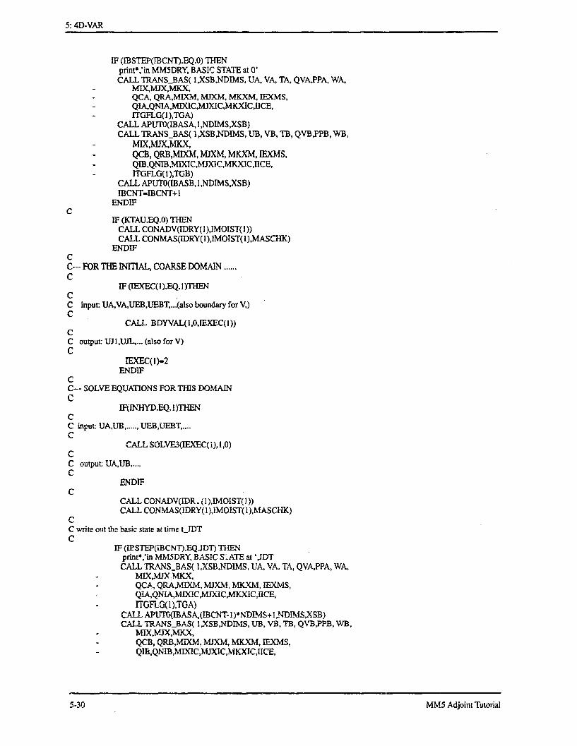
5: 4D-VAR

IF (IBSTEP(IBCNT).EQ.0) THENprint*,'in MMSDRY, BASIC STATE at O'CALL TRANS_BAS( 1,XSBNDIMS, UA, VA, TA, QVA,PPA, WA,

MIXMJXMKX,QCA, QRA,MIXM, MJXM, MKXM, IEXMS,QQNIAAMIIC,MJXIC,MKXIC,ICE,ITGFLG(1),TGA)

CALL APUTO(IBASA, 1,NDIMSXSB)CALL TRANS_BAS( I ,XSBNDIMS, UB, VB, TB, QVBPPB, WB,

M- ,MJXMKX,QCB, QRB.MXM, MJXM, MKXM, EXMS,QIB,QNIB,MIX IC,MJXC,MKXIC,nCE,ITGLG(1),TGB)

CALL APUTO(IBASB, 1 NDIMSXSB)IBCNT-IBCNT+l

ENDIFC

IF (KTAUEQ.0) THENCALL CONADV(IDRY( ),IMOIST(1))CALL CONMAS(IDRY(1),IMOIST( ),MASCHK)

ENDIFCC--- FOR THE INIIAL, COARSE DOMAIN ......C

IF (IEXEC(1).EQ. I)THENCC input: UA,VA,UEB,UEBT,...(also boundary for V,)C

CALL BDYVAL( 0,IOEXEC(1))CC output UJ1,UJL,... (also for V)C

EXEC(1)-2ENDIF

CC-- SOLVE EQUATIONS FOR THIS DOMAINC

IFQtNHYD.EQ. !)THENCC input: UAUB, ... , UEB,UEBT,....C

CALL SOLVE3(fEXEC( 1), 1,0)CC output: UAJB,...C

ENDIFC

CALL CONADV(IDR .(I),IMOIST( ))CALL CONMAS(IDRY(1),IMOIST( ),MASCHK)

CC write out the basic state at time t JDTC

IF (ISTEP(iBCNT).EQJDT) THENprint*'in MM5DRY, BASIC S'ATE at ',JDTCALL TRANS_BAS( 1XSB,NDIMS, UA, VA. TA, QVA,PPA, WA,

MIXMJrX MKEX,QCA, QRA,VMIXM, MJXM, MKXM, IEXMS,QIAQNIAMIXICM C,_MKXIC,IICE,

- ITGFLG(),TGA)CALL APUTCBMASABCNT- l)*NDIMS+l ,NDIMSXSB)CALL TRANSBAS( 1,XSBNDMSl , UB, VB, TB, QVBPPB, WB,

- MIX,MX,MKX,- QCB, QRB,.MXM, MJXM MKXM,, IEXMS,- QIB,QNIB ICJMXIC-NICiKXICJICE,

5-3 MM5 Adon Tuora


5: 4D-VARC . .

- TGFLG(l),TGB)CALL APUT(IBASB,(IBCNT- )*NDIMS+ 1,NDIMS,XSB)IBCNT-IBCNT+1

ENDIFCC write out the forcing term and calculate the cost functionC

IF (ITSTEP(1,DCNT(1)).EQJDT) THENprint,'MMSDRY,OBS at JDT=',JDTCALL TRANSF( 1,XSNDIMSS, UA, VA, TA, QVA,PPA WA,

M- IXX ,MX X,QCA, QRAMIXM, MJXM, MXM, IEXMS,QIA,QNIAMlC MJXICMICMC ,IICE)

CALL AGET(IOBS(1),(IDCNT(1)-1)*NDIMOBSS+1,NDIMOBSSXSB(1))C

DO 80 I=1,NDIMSSXSB)=XSI)-XSB()

80 CONTINUEC

CALL AGET(IWGT,(IDCNT(l)-I)*NDSSDIMSS+,NDSSXS())00 81 I=1,NDIMSS

VAL(1)=VAL(1)+X XSB(W)*XS*XS(I)XSB(1)=2.0*XSB(I)*XS(I)

81 CONTINUECALL APUTO(IOUT(1),(TDCNT(1)-1))*NDIMSS+1NDIMSS,XSB(l))IDCNT(l)=IDCNT(l)+lprint *, 'at JDT'JDT,' VAL(1)=',VAL(1)

ENDIFC

10 CONTINUEC

PRINT *,NMBDY,' PERIODS BDY USED IN MMSDRY'print 55555,(VAL(I),I1 ,NOBSYPE)

55555 format(1x,'VAL-', 12(E14.5,5x))TVAL-O.DO N-,NOBS_TYPETVAL-TVAL+VALN)ENDDORETURNEND

5.9 The MM5 adjoint model subroutine incorporated with the forcing

terms a (calculated in mm5dry.F): adjdry.Fax(t)

SUBROUTINE ADJDRY(IOUT)cccccccccccccc CCCCCCCCCCCCCCCCCCCCCCCCCCCCCCCCCCCCCCCCCCCCCCCCCCCCCCCCC!!!! THIS IS TH TANGENT LINEAR MODEL OF THE ADIABATIC VERSION of MMl5C moisture variable QV, diffusion, bulk PBL includedCC output initial conditions: UA,VATA,QVA,PPA,WAC boundary conditions: FSBCFNBC,FWBCFEBC,FSBTC,FNBTC,FWBTC,FEBTC F represents U,V,T,Q,PP,WC input forecasted model state: UA,VATA,QVAPPAWACcCCCcccccccc CCCCCCCCCCCCCCCCCCCCCCCCCCCCCCCCCCCCCccc CCCCCCCCC# include <parame.incl>


5: 4D-VAR

# include <parmin.incl># include <param2.incl># include <param3.incl># include <bcontrol.incl># include <dusolvel.incl># include <addrO.incl># include <various.incl># include <point3d.inc># include <pointbc.inci># include <nonhydbincl># include <nonhyd.incl># include <minim.incl># include <point2d.incl># include <varia.incl># include <nlsol9.incl># include <addr29.incl># include <uprad.incl>C

CDIMENSION AUA(MIX,MJX,MKX),AVA(MIX,MJX,MKX),ATA(MIX,MJX,MKX),- AQCA(MIXM, MJXM,MKXM ), AQRA(MIXM, MJXM, MKXM),- AQIA(MIXIC,MJXIC,MKXIC),AQNIA(MXIC,MJXICMKXIC),- ATGA(MIX ,MX ),

- AQVA(MIXMJX,MKX)APPA(MIX,MJXMKX)AWA(MIXMXKXP INNH)COMMON /SCRTCH/XSB(NDIMSBB)BXS(NDIMS),

2 ZZZ(NSCRTCHI-NDMSBB-NDMS)c DIMENSION IDCNT(NOBSTYPE),IOUT(NOBSTYPE)

DIMENSION IOUT(NOBS_TYPE)C

INTEGER EXEC(MAXNES)CHARACTER FILENAME*9

CC initializeCc duo to Kuo scheme

DO 873 J-I,MJXDO 873 I-I,MIX

RA!NC(IJ)-O.RAINNC(IJ)-0.

873 CONTINUEc

DO J-6,6DO 1-6,6

TMASK(IJ)-0.ENDDOENDDO

cIDCNT(I)-NOBSIBCNT-NBAS-IBASESAVE-IBCNTGVALO.NB=NMBDYIEXEC(I)-2

CC zero "initial" condition for the adjoint model integrationC This part is not in the adjoint model checking, it should be hereC if we want to calculate the gradientc

CALL ZEROVARIABLE(UA, VA, TA, QVAPPA, WA,- MIX,MJX,MKX,-QCA, QRA,MIXM, MJXM, MKXM, IXMS,- QIA,QNIAMXIC,MJXIC,MKXIC,HCE,-ITGFLG(l),TGA)

5-3 MM Adjin TutorI~ial


5: 4D-VARI . .... . _r _ __

CALL ZEROBDYc

CALL ZERO_VARIABLE(UB, VB, TB, QVB,PPB, WB,-MIX,MJX,MKX,

- QCB, QRB,MIXM, MJXM, MKXM. IEXMS,- QIB,QNB,MIXIC,MXIJXMKXIC, CE,

- ITGFLG(1),TGB)CC zero-out UJL,....C

DO 6000 K-1,MKXDO 6000 -1,MIX

UJ11 (I,K)-0.UJL (I,K)O.UJ2 (IK)0.UJLX(I,K)-0.

CVJI (I,K5=0.VJL (I,K)-O.VJ2 (IK)0.VJLX(I,K)-0.

6000 CONTINUEC

DO 7000 K-1,MKXDO 7000 J-1,MJX

ulI (tK)-0.UL (J,K)-0.UI2 (J,K)-0.UILX(J,K)=0.

CVII (JKC0.VIL (JK)-0.V2 (J,K)O0.VILX(J,K)-0.

7000 CONTINUEc

CALL MINIT(- !)C

L2D-MIX*MJXL3D1MIX*MJX*MKXL3DNHr MIXNH*MJXNH*MKXNHL3DNHP-MIXNH*MJXNH*KXP NH

print*,' MIMB DY-',ITIMBDYC

WRITE (FILENAME(I:9),'(A6,3.3)') 'LBC'NBprint *,' GET BDY FROM ',FIENAMECALL BDY_STORE(- I LENAMENB,

I UWB9, UEB9, USB9, UNB9,2 VWB9, VEB9, VSB9, VNB9,3 TWB9, TEB9, TSB9, TNB9,4 WWB9, WEB9, WSB9, WNB9,5 QWB9, QEB9, QSB9, QNB9,6 PPWB9, PPEB9 B9, 9PPNB9,7 QCWB9. QCEB9, QCES9, QCNB9,8 , REB9, QRSB9, QRNB9,9 QIWB9, QIEB9, QISB9, QINB9,& QNIWB9,QNIEB9,QNISB9,QNINB9,1 MIX, MJX, MKX,MIXNH, MJXNH, MKXNH,.KXP1NH, NSPGD,2 MIXM, MJXM,MKXM,MIIC MJXIC, MKXIC, NSPGX,3 EXMS,IICE)

WRITE (FILENAME(1:9),'(A6,13.3)') 'LBCT_.'NB

MM Adjin Tuoia 5-33I · I. L I~-L II


5: 4D-VAR

print *,' GET BDY tendency FROM ',FILENAIMECALL BDYSTORE(- 1,FHENAMENB,

1 UWBT9, UEBT9, USBT9, UNBT9,2 VWBT9, VEBT9, VSBT9, VNBT9,3 TWBT9,TEBT9, TSBT9, TNBT9,4 WWBT9, WEBT9, WSBT9, WNBT9,5 QWBT9, QEBT9, QSBT9, QNBT9,6 PPWBT9, PPEBT9, PPSBT9, PPNBT9,7QCWBT9,QCEBT9, QCSBT9, QCNBT9,8 QRWBT9, QREBT9, QRSBT9, QRNBT9,9 QIWBT9, QIEBT9, QISBT9, QINBT9,& QNIWBT9,QNIEBT9,QNISBT9,QNINBT9,1 MIX, MIX, MKX,MIXNH, MJXNH, MKXNH,KXPIN, NSPGD,2 MIXM, MJXM,MKXM,MXIC, MJXIC, MKXIC, NSPGX,3 IEXMS,HCE)

cprint*,'in ADJMOD, MAXSTP=',MAXSTPDO 0 JDT-MAXSTP, 1,-I

CIF (IBSTEP(IBCNT).EQJDT-I) TEN

print*,' get IBASA, IBCNT-',IBASA, IBCNTCALL AGETOIBASA,(IBCN I)*NDIMS+INDIMS,XS)CALL TRANS 3AS(- I XSNDIMS, UA9, VA9, TA9, QVA9,PPA9, WA9,

-MIX,MJXKX.- QCA9, QRL9,MIXM, MJXM, MKXM, IEXMS,- QIA9,QNIA9,MIXIC,MJXIC,MKXIC,ICE,

r- rGFLG(!),TGA9)print*,' get IBASB, IBCNT-',BASB, IBCNTCALL AGETO(IBASB,(fBCNT- 1)*NDIMS+ ,NDIMSXS)CALL TRANS_BAS(-I,XS,NDIMS, UB9, VB9, TB9, QVB9,PPB9, WB9,

- MIXMJX.MKX,- QCB9, QRB9,MIXM, MJXM, MKXM, IEXMS,- QIB9,QNIB9,MIXIC,MJXIC,MKXIC,IICE,

-ITGFLG(I),TGB9)IBCNT-IBCNT-1IBASE SAVE-IBCNT

ENDIFCCAA_ AAA___AAAAAAAAAAA AAAAAA AAAAAAA

C forcing term due to direct obs M "AAAAA^^

"A ^ "-

CIF (ITSTEP(l,IDCNT(l)).EQJDT) THEN

print*,'ADJMM,Forcing at JDT='JDTCALL AGETOIIOUT(),(IDCNT(l)-l)*NDIMSS+lI,NDIMSSXSB(l))CALL TRANSF(-1,SBNDIMSBBAUAAVAATA,AQVA,APPAAWA,

- MIXMJXIX,- AQCA, AQRAMIXM, MJXM, MKXM, IEXMS,

- QAIAQNIAMIXIC,MJXICMKXICCE)C

DO 4000 J=1MJXDO 4000 K=,MKXDo 4000 I=1MX

UA (IJK-AUA (IJK)+UA (IJ)VA (IJK)AVA (IJ)+VA (K)

4000 CONTINUEDO J=1MX-1DO K=1,MKXDO I=1,MIX-1

TA (UJK ATA (IJt)+TA lJK)QVA(UI )=AQVA(JK)+QVA(, K)

ENDDOENDDOENDDO


5: 4D-VAR_~~ ~ ~ ~ ~ ~ ~~~~~~~~~~~~~~~~~~~~~~~~~~ . I I I _ _

IF (IEXMS.EQ.1) TEENDO J=1,MJX-IDO =1,MKXDO I=1,MlX-1

QCA(IJK)=AQCA(,JK)+QCAaJ,QRA(IJK)AQRA(fJK)+QRA(IJK)

ENDDOENDDOENDDO

IF (IICEEQ.1) THENDO J=,MJX-1DO K=1,MKXDO I=1,MX-

QIA(IJ,KJ= AQIA(I,J)+ QIA(IK)QNi(I,,)=AQNIA(IJ)+QNIA(IJK)

ENDDOENDDO

ENDIFENDIF

CDO 50 J=1,MJXNH-1DO 5000 KIMKXNHDO 5000 I=1,MXNTH-

PPA(IJK)=APPA(,K)+PPA(JK)5000 CONTINUE

DO 6002 J-=,MJXNH-DO 6002 K=2,KPINH-1DO 6002 i-,MIXNH-1

WA(IJK)=AWA(IJ,)+WA(IJ^)6002 CONTINUE

IDCNT(1)sIDCNT(1)-1print*'ADJMM,Forcing at JDT='JDT,' end.'

END IFCt- AJ AAAAAAAAAAAAAAAAAAAAAAAAAAAAAAAAAAAAAAAAAAAAAAAAAA

c added due to more than one boundary conditionc

IF (NB.EQ. 1) THENTBDYBE - 0.0

ELSETBDYBE - TIMBDY(NB-1)

ENDIFBDYTIM TIMBDY(NB)

c adding endsC

IF (JDT.EQ.1) THENC input: UA9,VA9,UEB9,....

EXEC(I)-1SXTIME-XTIMEXTIMhEO.CALL MBDYVAL(1,0,IEXEC(1))IBXEC(l)-2XTIME-SXTIME

C output: UJ19......C

ELSEC The last part in SOLVE3CC HSCR 1 in VARIA, PSA in POINT2D, ILJL in VARIOUSCc print*, ,LJKLILXJLX,ILJL,KL,XIXJLX

CALL DOTS(PSA,HSCR I,ILJL,MIX,MJX)C

MM5I, Adjin Tuora 5-35C·--_


5: 4D-VAR

DO 820 K=1,KLDO 800 I-1,L

UJ19(I,K)=UA9(I, 1 ,K)HSCR1 (1, 1)VJ19(I,K)-VA9(I 1,K)/HSCR1(,l )UJL9(I,K)-UA9(IJL,K)HSCR (IJL)VJL9(,K)-VA9(IJLKyHSCRI(IJL)UJ29(I,K)-UA9(I,2,K)/HSCR (I,2)VJ29(I,K)-VA9(1,2,K)/HSCR1(I,2)UJLX9(I,K)=UA9(I,JLX,KHSC 1 (IJLX)VJLX9Ct,K)-VA9(IjLX,Ky)HSCRIJ 1JX)

800 CONTINUEDO 810J-IJL

Ul19(J,K)=UA9( ,J,K)HSCR 1(1 J)VI19(JK)VA9( 1 J,K)/HSCR I (1J)UIL9(J,K)-UA9(ILJ,KHSCR (IL,J)VIL9(J,K)-VA9(ILJ,K)HSCR 1 LJ)UI29(J,K)-UA9(2J,K)/HSCR1(2J)V129(J,K)-VA9(2,J,K)HSCR 1(2J)UILX9(J,K)-UA9(ILXj,KHSCR 1 (ILXJ)VILX9(J,K)-VA9ILXJ,KYHSCR 1 (1 XJ)

810 CONTINUE820 CONTINUE

CC output UJ19.....

ENDIFCC

IF (INHYD.EQ.)THENC

CALL ASOLVE3(IEXEC(I), ,0)C

ENDIFC

IF (JDTEQ. 1) THENprint*'CALL ABDYVAL'IEXEC(1)-ICALL AGETO(IBASA, 1DIMS,XS)CALL TRANS_BAS(- IXS,NDIMS, UA9, VA9, TA9, QVA9JPPA9, WA9,

M- X,MJX,MKX,QCA9, QRA9,MIXM, MJXM, MKXM, IEXMS,QIA9,QNIA9,MIXCJXXIC,MKXIC,HCE,ITGFLG(l),TGA9)

CALL ABDYVAL(1,0JEXEC(1))ENDIF

CIF(NB.GT.0) THENIF (JDTEQ.IIMBDY(NB)) TEN

print*,'save gradient of J with respect to LBC at NB-',NBWRITE (FILENAME(I:9),'(A6,3.3)') 'GLBC_',NBCALL BDY_STORE( IJILENAME,NB,

I UWBT, UEBT, USBT, UNBT,2 VWBT, VEBT, VSBT, VNBT,3 TWBT, TEBT, TSBT, TNBT,4 WWBT, WEBT, WSBT, WNBT,5 QWBT, QEBT, QSBT, QNBT,6 PPWBT, PPEBT, PPSBT, PPNBT,7 QCWBT, QCEBT, QCSBT, QCNBT,8 QRWBT, QREBT, QRSBT, QRNBT,9 QIWBT, QIEBT, QISBT, QINBT,& QNIWBT,QNIEBT,QNISBTQNINBT,I MIX, MJX, MKX,MIXNH, MJXNH, MKXNH,KXPINH, NSPGD,2 MIXM, MJXM,MKXM,MIXIC, MJXIC, MKXIC, NSPGX,3 IEXMS,IICE)

c

5-3 MM Adoii Tutorial -.-MM5 Adjoint Tutorial5-36

5: 4D-VAR

CALL ABDY_UPDATE(NB)CALL ZEROBDY

CNB-NB-1IF (NB.GT.0) THEN

print *,'get BDY9 from LBC.',NBWRITE (FILENAME(I:9),'(A6,I3.3)') 'LBC.',NBCALL BDY_STORE(- FILENAMENB,

1 UWB9, UEB9, USB9, UNB9,2 VWB9, VEB9, VSB9, VNB9,3 TWB9, TEB9, TSB9, TNB9,4 WWB9, WEB9, WSB9, WNB9,5 QWB9, QEB9, QSB9, QNB9,6 PPWB9, PPEB9, PPSB9, PPNB9,7 QCWB9, QCEB9, QCSB9, QCNB9,8 QRWB9, QREB9, QRSB9, QRNB9,9 QIWB9, QIEB9, QISB9, QINB9,& QNIWB9,QNIEB9,QNISB9,QNINB9,1 MIX, MJX, MKX,MIXNH, MJXNH, MKXNH,KXP INH, NSPGD,2 MIXM, MJXM,MKXMMIXIC, MJXIC, MKXIC, NSPGX,3 IEXMS,IICE)

CWRITE (FILENAME(1:9),'(A6,13.3)') 'LBCT_,NBCALL BDY_STORE(-1 ,FILENAMENB,

1 UWBT9, UEBT9, USBT9, UNBT9,2 VWBT9, VEBT9, VSBT9, VNBT9,3 TWBT9, TEBT9, TSBT9, TNBT9,4 WWBT9, WEBT9, WSBT9, WNBT9,5 QWBT9, QEBT9, QSBT9, QNBT9,6 PPWBT9, PPEBT9, PPSBT9, PPNBT9,7 QCWBT9, QCEBT9, QCSBT9, QCNBT9,8 QRWBT9, QREBT9, QRSBT9, QRNBT9,9 QIWBT9, QIEBT9, QISBT9, QINBT9,& QNIWBT9,QNIEBT9,QNISBT9,QNINBT9,I MIX, MJX, MKX,MIXNH, MJXNH, MKXNH,KXPINH, NSPGD,2 MIXM, MJXM,MKXMMIXIC, MJXIC, MKXIC, NSPGX,3 IEXMS,CE)

cENDIF

CENDIFENDIF

CC

10 CONTINUECc

CALL AXA2XB(ILJL)CALL AREMOVE NEGATIVE(QVA,QCA,QRA,QIA,QNIA,IEXMS,IiCE,

- MIX,MJX,MKX,MIXM,MJXMMKXM,MIXIC,MJXIC,MKXIC,- ~IQINDX,IQCINDX,IQRINDX,IQIINDX,IQNIINDX)

CALL AUA2UEBCALL AWBC

Cprint'*save gradient of J with respect to LBC at NB=',NBWRIE (FILENAME(1:9),'(A6,I3.3)') 'GLBC_.',NBCALL BDY_STORE( ,FILENAM,NB,

1 LUWBT, UEBT, USBT, UNBT,2 VWBT, VEBT, VSBT, VNBT,3 TWBT, TEBT, TSBT, TNBT,4 WWBT, WEBT, WSBT, WNBT,5 QWBT, QEBT, QSBT, QNBT,6 PPWBT, PPEBT, PPSBT, PPNBT,7 QCWBT, QCEBT, QCSBT, QCNBT,8 QRWBT, QREBT, QRSBT, QRNBT,

MMS Adjoint Tutorial 5-35-37MM5 Adjoint Tutorial

5: 4D-VARr

9 QIWBT, QIEBT, QISBT, QINBT,& QNIWBT,QNIEBTQNISBTQNINBT,1 MIX, MJX, MKX,MIXNH, MJXNH, MKXNHKXP1NH, NSPGD,2 MIXM, MJXMMKXM,MIXIC, MJXIC, MKXIC, NSPGX,3 IEXMS,IICE)

CC forcing term at the initial timet MeA,,.AAAAAAAAA",.^C

IF ((ITSTEP(1IDCNT(l)).EQ.O)AND.(IDNT(T).GT.O)) THENprint*,'MMSADJ, Forcing at JDT=O'

CALL AGETOIOUT(l(IDCNT(l)-l)*NDIMSlDIMSASB(l))CALL TRANSF(.-,SB,NDIMSBBAUAAVAATA,4QVAAPPAWA,

MIEXJXdKXtAQCA, AQRAXM, MJXM MKXM, IEXMS,AQIAAQNIA,MIXICMJXIC,MKXIC,HCE)

DO J=1,MJXDO K=1,MKXDO I=INMIX

UA (IJK)=AUA (I,J,K)+UA (IJ,)VA (IJ,)=AVA (I,JK+VA (IJK)

ENDDOENDDOENDDODO J-1,MJXI-DO K=l,MKXDO I=1,MIX-1

TA (IJK)ATA (IJK)+TA (JK)QVA(I,J,)=AQVA(IlK)+ QVA(IJK)

ENDDOENDDOENDDO

IF (IEXMS.EQ.1) THENDO J=,MJX-1DO K=1,MKXDO I=,MIX-1

QCA(JJIOAQCA(IJK)QCAqJK)QRA(IJ,K)=AQRA(IJ,)+QRA(IJK)

ENDDOENDDOENDDO

IF (IICE.EQ.1) THENDO J=1,MJX-1DO K=IMKXDO I=l,MIX-1

QIA(IJK)= AQIA(IJ^)+ QIA(I,,K)QNIA(IJ,)=AQNIA(I,)+QNIA(IJX

ENDDOENDDOENDDO

ENDIFENDIF

CDO J= I.MJXNH-1DO K=1JKXNHDO I=1,MIXNH-1

PPA(IJ,)=APPA(IJX+PPAI,J,K)ENDDOENDDOENDDODO J=,MJUXNH-1DO K=2KXP1NH-1DO I=IIXNH-1

WA(IJ)=AWA(IK)+WA(IJK)


5: 4D-VAR

ENDDOENDDOENDDO

CEND IF

cC AAAAAAAAAAAAAAAAAAAAAAAAAAAAAA hAAAA AAAAAAAAAAA

CC check to see whether the norm of gradient is too smallC

CALL TRANSF( 1,XSB,NDIMSBB,UA,VA,TA,QVA,PPA,WA,- MIX,MJXMKX,- QCA, QRA,MIXM, MJXM, MKXM, IEXMS,- QIA,QNA,MIXIC,MJXIC,MKXICCE)

DO 5 I-1,NDIMSBBGVAL=GVAL+XSXSBI)*XSB

5 CONTNUEPRINT *,'GRADIENT - ',GVALIF(GVAL.LT. I.F-10) THEN

PRINT *,'GRADIENT REDUCED BELOW 1.E-10'STOP

END IF

RETURNEND

MM5I Adon Tutorial 5-395-39MM5 Adjoint Tutorial

5: 4D-VAR, ._,

I UlJ

c 1000000C

c

e4-CO0

0 5000

Iterations.·0400

3004.C

12c 2000E

100

O0 5 10 15

Iterations20 25 30

Figure 5.1 Variation of the values of the cost function (upper panel) and the normof the gradient with respect to the ICs (lower panel) with the number of iterations.


4 CrLt

I


5: 4D-VAR

i=-e 3 " .I:- ; s _s s= ;;

0000 UTC 13 March

~M Is Km -t I arm:tIS W:

, M i. I o ' l I tV y I _ I. I ffI,

0300 UTC 13 March

* 2 r l 2 . r t ~ I i t Z t 'D I 3 t I = :-

0600 UTC 13 March

Mi I = tLL.z: tin : att I =' I,= -it w z tI: I st =:

1200 UTC 13 March

Figure 5.2: Errors in the wind fields at a = 0.65 at the Oth (left column) andand 15th(right column) iteration from 0000 UTC 13 March to 1200 UTC13 March 1993. Contour interval is 0.5 m/s.

M M 5~ ~ ~ ~~ ~~ ~~~ ~ ~ ~~ ~ ~ ~ ~ ~ ~ ~ ~ A j i n, T o i a

5 -4 1

.01 Of liwl All. A u.9 95

I r*\ ··CI · · 4~J~' C~~v ~Ti, ~ e up

r~LU~r-· C~·~·5 e~~~L~ I ~ ~ ~ MD

r II*I I 1· ~ ~ P~ L~ L ~ an

r · ~U-Y _L· · ·~ (I) MT mg v

ti k ' , t '1 .b u- *. . * I U . - vo _ w

.ff Iv , . I1-;~~~~~~~~~~~;

11I

rer-�r I.�rl��iY�t·P-�LUI

;II I I rt · · ·)I CL-_P��I�9��? r·rt

I1·slss. I·)c�r;r'�i�ZP·- ·G ·aii�··ci···�

�-r�rrr

· · · · · r1(\��9��9Bt �rr*CI

+I

ry IIi � r�e , �·�� 3·

; ·,·�c�S��`--l�t..C;rO

�I

L L�'�r r\� y* · ·

r · �1· · r It · · ·1· I FI ��L�U t�C·l I I�llll'\r

s i' f r r r I I· r·; 1.9·�1�U�Y��btfllr� ��

rl�Ytlil�rlr�·�Y �+·(�--�c�·�rSH·''· I··�//�U�

1PITt t ·/5 1�1 /L �t I �L�· ,· · Cu;l r II� r � I N J-· \ · �/ Ai� 1 i t � -· ·) ·

r�AI-L I �� · · · �C

· � � ��, r r ��C'r · rl .'tl�t · · ·

slt· · �J· -I· · 11�C1�11�-��·3·\··

r···l�···· ·I· ·d·. I · I� r L · I -· I,�· L · · ·�- C

F-M I I."w == : = :=_

S II

14 a_ r · u~ r·· ~ · Lr

- - - m '- -· -I$- -6=-

IM

-.1 .1

aIa*

*I

so1

mU

as

as

Ia.

5-41MM5 Adjoint Tu~torial

460

ON

am

am

ml

::::;

\II

Jl\��c�r·L,,,-*7--G·J. I·l�-aa�rGr···\·�lr� -*·4 �'' 4t � ��CLJ I KI

r 1 PYI \·

· L4Lt�t�t�t�t�t�t�t�t�t�t�t�t�t�t�t�t�t�

.,,,,��, �·�1·�1�.. r)\*\

/r��yiLl�pe�;RL�irrrr�-(LI

·L · IrF -C ·. r I r w�� .P-Y r r r 41 ' 'mr � -I- · ·r L �LE f � �� 1 ·\· .. 1

/�cr

0000 UTC 13 March

0300 UTC 13 March

0600 UTC 13 March

1200 UTC 13 March

Figure 5.3: Same as Figure 5.2 except for the temperature field at a = 0.85. Contourinterval is l.0 K.

5-42 MM Ador Tuora

5: 4D-VAR

a 4_ ii . . _w ._ W

> _ U _


5: 4D-VAR

MM Adon Thoil54 5-43.MM5 Adjoint Ttorial

5: 4D-VAR_ _ _I

5-4 MM djithora


6: CONCLUSION-~~~~~~~~~~~~~~~~~~~~~~~~~~~~~~~~~~~~~~~~~~~~~~~~~~~~~~~~~~~~~~~~~~~~~~m

CONCLUSION- = - m m m a :aa as a a -i ~

Numerical efficiency 6-3

Observation operators 6-4

Adjoint physics 6-4

Background information 6-5

MM5~ Adon Tuoia -


6: CONCLUSION

MM5~ Adjin Tuora 62


6: CONCLUSION

Conclusion

,1 -~ .1111 111111 RI 1111 1I ll 1 11ll 1111 1111 Y ll

The MM5 tangent linear and adjoint models can be used for a wide range of applications (seeZou et al. 1997 for a review of the most important ones). Users can make use of these tools andand adapt them to the kind of research they are interesting in. However, it is important to realizethat, although the MM5 adjoint modeling system is a highly powerful research tool, we do nothave a complete MMS5 4-dimensional variational data assimilation system (MM5 4D-VAR sys-tem). Additional work is needed to build a complete and robust data assimilation system. Severalproblems still need to be solved before we can make the MM5 4D-VAR system a communitymesoscale data assimilation system. These issues are numerical, physical and statistical. Follow-ing are the most important ones (that we plan to work on) in the up-coming years.

6.1 Numerical efficiency

With the present version of the code, the costs of the MM5 tangent linear and adjoint modelintegrations are about 2.7 and 6.9 times that of the MM5 forward model integration, respectively.The large CPU requirement in the MM5 adjoint model is caused by the J-slide structure in theMM5 model in solve3.F and the principle we used in the tangent linear and adjoint model devel-opment. We use minimum disk space and internal memory for saving the basic state information,which causes many repeated basic state calculations. Since at least one forward MM5 and onebackward MM5 adjoint model integration is needed for every iteration in a minimization proce-dure, this may represent too high a computational requirement for many users who wish to use thesystem. It is clear that the numerical efficiency of the adjoint code that is presently released needsto be improved.There are several ways to improve the efficiency of the adjoint code: (i) change thedynamical structure of the MM5 model; (ii) multi-task and vectorize the MM5 adjoint model; (iii)improve the efficiency of the minimization procedure, and (v) adapt an incremental approach.

The computational cost of integrating the MM5 adjoint model can largely be reduced with theuse of a code optimizer. A preliminary result of parallelizing the MM5 adjoint code reduced theCPU time of the adjoint model integration by half. Another way to reduce the computational costof 4D-VAR is to improve the efficiency of the minimization procedure. This can be realized by theuse of preconditioning matrices. At each iteration these matrices are applied to the gradient so thatthe new descent direction is more efficient than the original descent direction before transforma-tion.This allows the minimization procedure to reach the minimum of the cost function with lessiteration than a minimization without preconditioning. The best preconditioner is the inverse ofthe Hessian matrix, which is, however, not accessible and can certainly not be fully inversed dueto its large dimension for a primitive equation model like MM5. Preconditioning matrices, there-

MM5 n r _

MIM5 Adjoint Tutorial 6-3

6: CONCLUSION

fore, must be estimated according to the problem that has to be solved.

The efficiency improvement that will result from vectorization, multitasking and precondi-tioning will not, however, be enough to allow any kind of high resolution experiments such ascloud-scale Doppler radar data assimilation. For that type of research, the assimilation algorithmshould be modified and some approximations would inevitably be necessary. One very interestingapproach is the so-called incremental approach. In this approach the nonlinear model is only usedto define the basic-state trajectory while the tangent linear model is used in conjunction with theadjoint in the minimization loop. Both the tangent linear and adjoint models are used either with alow resolution or with degraded physics, requiring much less CPU time than models with full res-olution and physics. This gain in computational cost is amplified by the iterative nature of theminimization process, which only uses the low-cost degraded tangent linearand adjoint models. Some operational centers have estimated that one order of magnitude reduc-tion of the computational cost can be expected by using such an approach when combined with agood preconditioner. From a technical point of view, the incremental approach can be easilyimplemented. It suffices to replace the nonlinear model with its tangent linear approximation inthe minimization routines.

6.2 Observation operators

In the standard code which is being released at the first MM5 adjoint tutorial, only directobservations (model variables) are assimilated into the MM5 model. However many indirectobservations (diagnostic quantities which are nonlinear functions of model variables) such as sat-ellite radiances, surface rainfall amount, precipitable water, and radar reflectivity data are, or willbe, available on a routine basis for mesoscale studies. In order to make use of these sources ofobservational information, various observational operators need to be developed along with theiradjoint counterparts. This means that for each kind of data, a numerical operator that representsthese observations from the MM5 model variables must be developed and its tangent linear andadjoint operators coded. The MM5 Adjoint Modeling System Group is currently working on theassimilation of five different kinds of indirect observations:

1) GPS/MET radio occultations,2) GPS precipitable water profiles,3) Doppler radar observations,4) Surface rainfall observations, and5) Satellite radiances

It is hoped that this research will lead to the development of a series of observation operators andenable us to incorporate more observations into the MM5 model. This new software, and thatdeveloped by outside users, will be added to the present version of the MM5 adjoint modelingsystem as soon as it becomes available and well-tested.

6.3 Adjoint physics

The current version (released in the summer of 1998) of the MM5 adjoint modeling systemincludes model dynamics, horizontal and vertical diffusions, a bulk PBL process, dry-convectiveadjustment, grid-resolvable precipitation, the Kuo cumulus parameterization, surface friction, a

6-4 ~1~~~ MM5-9--~~~~~~ AdjI TI toial

64 MMt5 Adjoint lb~torial

p

P 6: CONCLUSIONp i _ -- _, --- _,-

p

P time-splitting scheme, and surface fluxes.p

p The tangent linear and adjoint operators of the following physical processes have already beenp developed, tested, and used for a few case studies: the adjoints of the Grell cumulus parameteriza-

tion; a microphysics scheme (Dudhia's scheme), and a high-resolution PBL scheme (the Blacka-dar scheme). These physical processes need further testing before they can be released for moregeneral use.

6.4 Background information

The current MMS adjoint modeling system does not have the necessary error statistics. Werealize that the background field and its error covariance matrix is crucial information to ensuresuccessful data assimilation, especially when sufficient observations are not available.The back-ground term in the cost function for mesoscale data assimilation needs to be developed, and itsimportance needs to be assessed. With the desire to apply the MM5 adjoint modeling system overa wide range of horizontal grid sizes and scales and over a wide range of geographical locations,as with the MMS model, the development of a proper background term for the MM5 assimilation4D-VAR system is a highly challenging task. This background term is also the basis for buildinga 3D-VAR system which may be preferably used in operational or real-time data assimilationexperiments due to its low computational cost. The 3D-VAR system may replace some of the pre-processing in the MM5 modeling system. Such an effort is now being undertaken by MPG/MMM/NCAR.

The development of the MM5 4D-VAR system was a tremendous effort of many person-years.Most of the development effort was supported by external fundings. The MM5 4D-VAR systemas it stands now is a highly useful research tool for data assimilation research, sensitivity analysis,and dynamic studies. However, much work remains to be done in making the MM5 4D-VAR sys-tem a more complete data assimilation system, and in making it a versatile tool for mesoscaleresearch and semi-operational application. With this initial release of the MM5 4D-VAR systemto the community, we are encouraging user input and modification to begin at once. Future devel-opment and improvement of the system will depend heavily, not only on the personnel at NCAR,but also on the user community in keeping the MM5 4D-VAR system at the cutting edge ofmesoscale data assimilation area.

M I T 6-5

MM5 Aadjoint Tutorial 6-5

6: CONCLUSION......-

6-6 MMS Adjin Tutorial6-6 MM5 Adjoint Tutorial

References

References

Anthes, R. A. and T. T. Warner, 1978: Development of hydrodynamic models suitable for air pol-lution and other mesometeorological studies. Mon. Wea. Rev., 106, 1045-1078.

Dudhia, J., 1993: A nonhydrostatic version of the Penn State-NCAR mesoscale model: Validationtests and simulation of an Atlantic cyclone and cold front. Mon. Wea. Rev., 121, 1493-1513.

Grell, G. A., J. Dudhia and D. R. Stauffer, 1993: A description of the fifth-generation Penn State/NCAR mesoscale model (MM5). NCAR Technical Note, NCAR/TN-398+STR, 117 pp.

Zou, X., and Y.-H. Kuo, 1996: Rainfall assimilation through an optimal control of initial andboundary conditions in a limited-area mesoscale model. Mon. Wea. Rev., 124, 2859-2882.

Zou, X., Navon, I. M., Berger, M., Phua, Paul K. H., Schlick, T., and Le Dimet, F X. 1993.Numerical experience with limited-memory quasi-Newton andtruncated Newton methods.SIAM J. on Optimization, 3, 582-608.

Zou, X., R Vandenberghe, M. Pondeca and Y.-H. Kuo, 1997: Introduction to adjoint techniquesand the MM5 adjoint modeling system. NCAR Technical Note, NCAR/TN-435+STR, 117PP.

MMS Tuora R-lR-1MM5 Tutorial

User's guide to the MM5 adjoint modeling system.

Documents

Transcript of User's guide to the MM5 adjoint modeling system.