User’s guide to Bayesian Cultural Consensus Toolboxzoravecz/bayes/data/Articles/Users guide...

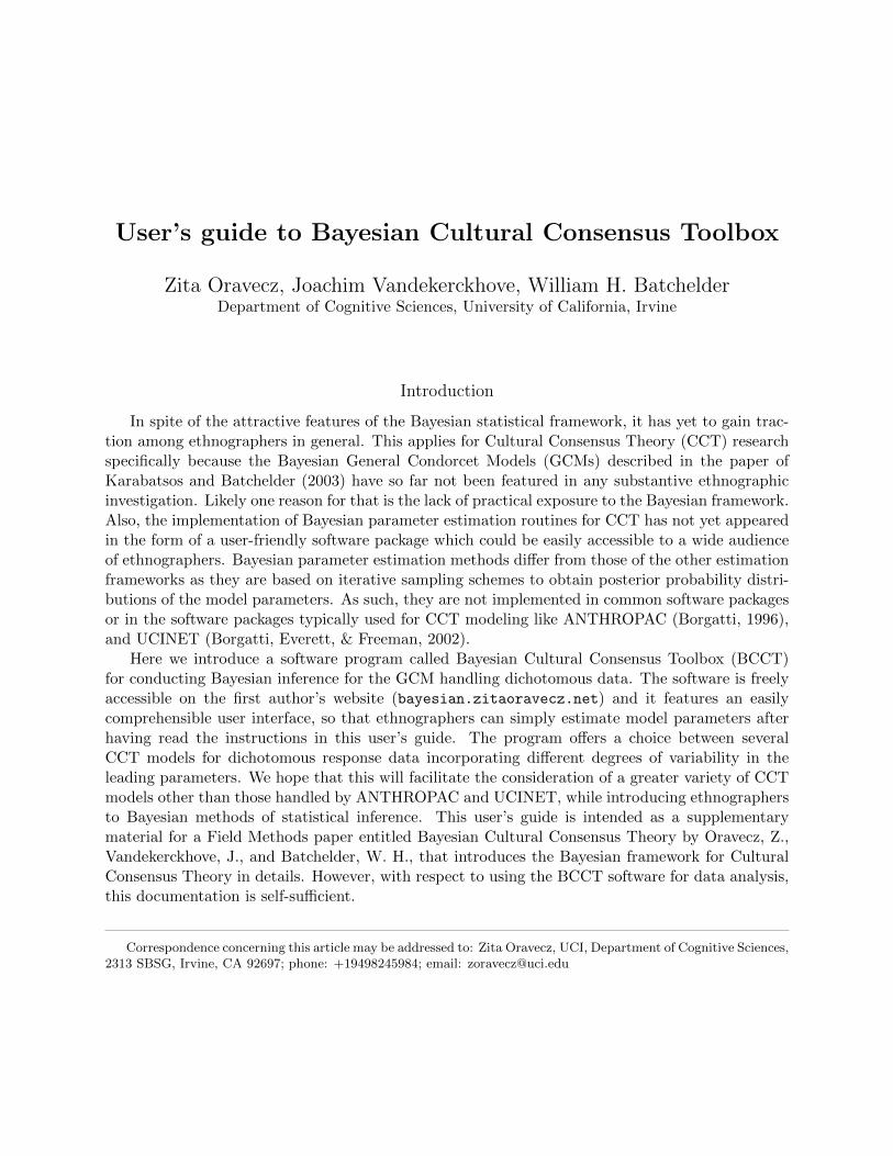
User’s guide to Bayesian Cultural Consensus Toolbox

Zita Oravecz, Joachim Vandekerckhove, William H. BatchelderDepartment of Cognitive Sciences, University of California, Irvine

Introduction

In spite of the attractive features of the Bayesian statistical framework, it has yet to gain trac-tion among ethnographers in general. This applies for Cultural Consensus Theory (CCT) researchspecifically because the Bayesian General Condorcet Models (GCMs) described in the paper ofKarabatsos and Batchelder (2003) have so far not been featured in any substantive ethnographicinvestigation. Likely one reason for that is the lack of practical exposure to the Bayesian framework.Also, the implementation of Bayesian parameter estimation routines for CCT has not yet appearedin the form of a user-friendly software package which could be easily accessible to a wide audienceof ethnographers. Bayesian parameter estimation methods differ from those of the other estimationframeworks as they are based on iterative sampling schemes to obtain posterior probability distri-butions of the model parameters. As such, they are not implemented in common software packagesor in the software packages typically used for CCT modeling like ANTHROPAC (Borgatti, 1996),and UCINET (Borgatti, Everett, & Freeman, 2002).

Here we introduce a software program called Bayesian Cultural Consensus Toolbox (BCCT)for conducting Bayesian inference for the GCM handling dichotomous data. The software is freelyaccessible on the first author’s website (bayesian.zitaoravecz.net) and it features an easilycomprehensible user interface, so that ethnographers can simply estimate model parameters afterhaving read the instructions in this user’s guide. The program offers a choice between severalCCT models for dichotomous response data incorporating different degrees of variability in theleading parameters. We hope that this will facilitate the consideration of a greater variety of CCTmodels other than those handled by ANTHROPAC and UCINET, while introducing ethnographersto Bayesian methods of statistical inference. This user’s guide is intended as a supplementarymaterial for a Field Methods paper entitled Bayesian Cultural Consensus Theory by Oravecz, Z.,Vandekerckhove, J., and Batchelder, W. H., that introduces the Bayesian framework for CulturalConsensus Theory in details. However, with respect to using the BCCT software for data analysis,this documentation is self-sufficient.

Correspondence concerning this article may be addressed to: Zita Oravecz, UCI, Department of Cognitive Sciences,2313 SBSG, Irvine, CA 92697; phone: +19498245984; email: [email protected]

BAYESIAN CULTURAL CONSENSUS THEORY 2

Introducing the Bayesian Cultural Consensus Toolbox through anexample dataset

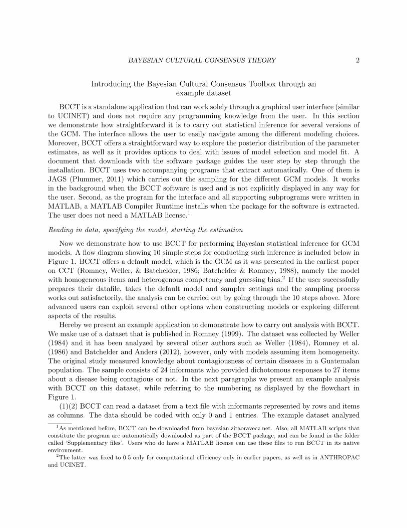
BCCT is a standalone application that can work solely through a graphical user interface (similarto UCINET) and does not require any programming knowledge from the user. In this sectionwe demonstrate how straightforward it is to carry out statistical inference for several versions ofthe GCM. The interface allows the user to easily navigate among the different modeling choices.Moreover, BCCT offers a straightforward way to explore the posterior distribution of the parameterestimates, as well as it provides options to deal with issues of model selection and model fit. Adocument that downloads with the software package guides the user step by step through theinstallation. BCCT uses two accompanying programs that extract automatically. One of them isJAGS (Plummer, 2011) which carries out the sampling for the different GCM models. It worksin the background when the BCCT software is used and is not explicitly displayed in any way forthe user. Second, as the program for the interface and all supporting subprograms were written inMATLAB, a MATLAB Compiler Runtime installs when the package for the software is extracted.The user does not need a MATLAB license.1

Reading in data, specifying the model, starting the estimation

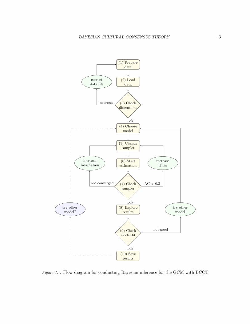
Now we demonstrate how to use BCCT for performing Bayesian statistical inference for GCMmodels. A flow diagram showing 10 simple steps for conducting such inference is included below inFigure 1. BCCT offers a default model, which is the GCM as it was presented in the earliest paperon CCT (Romney, Weller, & Batchelder, 1986; Batchelder & Romney, 1988), namely the modelwith homogeneous items and heterogenous competency and guessing bias.2 If the user successfullyprepares their datafile, takes the default model and sampler settings and the sampling processworks out satisfactorily, the analysis can be carried out by going through the 10 steps above. Moreadvanced users can exploit several other options when constructing models or exploring differentaspects of the results.

Hereby we present an example application to demonstrate how to carry out analysis with BCCT.We make use of a dataset that is published in Romney (1999). The dataset was collected by Weller(1984) and it has been analyzed by several other authors such as Weller (1984), Romney et al.(1986) and Batchelder and Anders (2012), however, only with models assuming item homogeneity.The original study measured knowledge about contagiousness of certain diseases in a Guatemalanpopulation. The sample consists of 24 informants who provided dichotomous responses to 27 itemsabout a disease being contagious or not. In the next paragraphs we present an example analysiswith BCCT on this dataset, while referring to the numbering as displayed by the flowchart inFigure 1.

(1)(2) BCCT can read a dataset from a text file with informants represented by rows and itemsas columns. The data should be coded with only 0 and 1 entries. The example dataset analyzed

1As mentioned before, BCCT can be downloaded from bayesian.zitaoravecz.net. Also, all MATLAB scripts thatconstitute the program are automatically downloaded as part of the BCCT package, and can be found in the foldercalled ‘Supplementary files’. Users who do have a MATLAB license can use these files to run BCCT in its nativeenvironment.

2The latter was fixed to 0.5 only for computational efficiency only in earlier papers, as well as in ANTHROPACand UCINET.


(1) Preparedata

(2) Loaddata

(3) Checkdimensions

correctdata file

(4) Choosemodel

(5) Changesampler

(6) Startestimation

(7) Checksampler

increaseAdaptation

increaseThin

(8) Exploreresults

try othermodel

(9) Checkmodel fit

(10) Saveresults

try othermodel?

ok

incorrect

ok

not converged AC > 0.3

not good

ok

Figure 1. : Flow diagram for conducting Bayesian inference for the GCM with BCCT


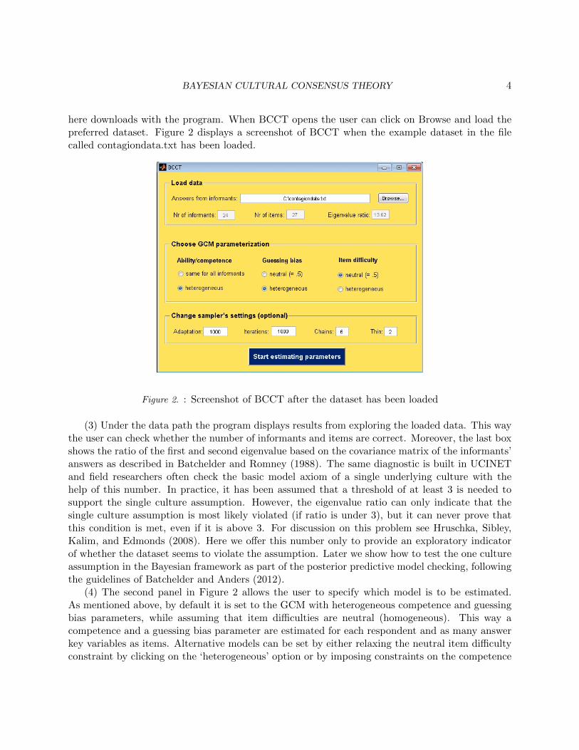
here downloads with the program. When BCCT opens the user can click on Browse and load thepreferred dataset. Figure 2 displays a screenshot of BCCT when the example dataset in the filecalled contagiondata.txt has been loaded.

Figure 2. : Screenshot of BCCT after the dataset has been loaded

(3) Under the data path the program displays results from exploring the loaded data. This waythe user can check whether the number of informants and items are correct. Moreover, the last boxshows the ratio of the first and second eigenvalue based on the covariance matrix of the informants’answers as described in Batchelder and Romney (1988). The same diagnostic is built in UCINETand field researchers often check the basic model axiom of a single underlying culture with thehelp of this number. In practice, it has been assumed that a threshold of at least 3 is needed tosupport the single culture assumption. However, the eigenvalue ratio can only indicate that thesingle culture assumption is most likely violated (if ratio is under 3), but it can never prove thatthis condition is met, even if it is above 3. For discussion on this problem see Hruschka, Sibley,Kalim, and Edmonds (2008). Here we offer this number only to provide an exploratory indicatorof whether the dataset seems to violate the assumption. Later we show how to test the one cultureassumption in the Bayesian framework as part of the posterior predictive model checking, followingthe guidelines of Batchelder and Anders (2012).

(4) The second panel in Figure 2 allows the user to specify which model is to be estimated.As mentioned above, by default it is set to the GCM with heterogeneous competence and guessingbias parameters, while assuming that item difficulties are neutral (homogeneous). This way acompetence and a guessing bias parameter are estimated for each respondent and as many answerkey variables as items. Alternative models can be set by either relaxing the neutral item difficultyconstraint by clicking on the ‘heterogeneous’ option or by imposing constraints on the competence


(same for all informants) and/or the guessing bias (neutral, i.e., fixed to 0.5) parameters. Forexample, if we change BCCT’s default model option by fixing the guessing bias to 0.5, we fit thesame GCM as UCINET and ANTHROPAC would fit but in the Bayesian statistical inferenceframework.

(5) The bottom panel Figure 2 contains the parameter settings for the sampler program thatdraws samples from the posterior distributions of the model parameters. The standard strategyis to use modern computational tools, called Markov chain Monte Carlo (MCMC) methods, todevelop a sampler that can generate many random values from the posterior distribution, and usethe sampled values to approximate the posterior distribution. Any MCMC sampler is designedto sample values of the parameters in proportion to how probable they are from the posteriordistribution. An extensive literature exists (see e.g., Robert & Casella, 2004; Gamerman & Lopes,2006) regarding simulation procedures to draw samples from any kind of distribution. Also, thereare available software packages that automate many of the steps required to run such a samplingprocedure. BCCT relies on one of these, namely JAGS. JAGS has built in heuristics to decideabout the most efficient MCMC algorithms to use for the specified models and most of the timeit is an amalgam of Metropolis-Hastings, Gibbs and slice sampling algorithms (Robert & Casella,2004).

The user has to decide only four options displayed in the bottom panel, however, most oftenthe already pre-filled values can work out satisfactorily, so the user can just leave those unmodifiedand click directly on the Start estimating parameters button. The reason for the options in thisrow is related to the standards for assuring the adequacy of the MCMC sampler which is discussedlater in the Exploring the results section. In the very first box, called Adaptation, we allocatea certain number of samples to be drawn but then discarded (not used to estimate the posteriordistribution), so they will not count towards our final posterior samples. The reason for thisadaptation period (most often called “Burn-in”) is twofold. First of all, the first sampled valuesof each sample chain are highly determined by their random starting values, and therefore do notrepresent the posterior distribution accurately. Second, during some initial period of sampling wewant the sampler program selected by JAGS to adapt its algorithms to find the most efficient one.For most CCT models the sampler needs around the first 1000 iterations to be discarded in orderto avoid the effects of the initial setting and allow JAGS to select an efficient sampler.

In the second box, called Iterations, the number of final (useable) posterior samples for eachchain is specified. It should be sufficiently large so that the sampler can explore the whole area of theconditional posterior densities of the parameters. Also, as mentioned above, this density explorationshould be restarted with different initial values to further ensure the sufficient exploration of theentire parameter space, and in the box called Chains we define how many times the explorations arerestarted. Our final posterior sample size is the product of these two. As a rule of thumb, 6 chainswith a minimum of 1000 useable samples each should be sufficient in most cases. Finally, the verylast box concerns the autocorrelation in the chains. Posterior inference should be based on chainsthat have little or no autocorrelation, so that we can be sure that each area of the posterior densityis equally likely to be represented in our final posterior sample. The way the Thin box controls theautocorrelation is the following: it keeps only every kth sample and discards the others, this waydecreasing correlation between the new neighboring samples. So if we put 1 in that box, that meansthat we do not thin and we keep every sample after the adaptation period. If we put 2 (default


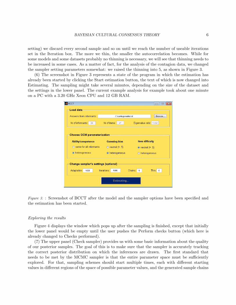
setting) we discard every second sample and so on until we reach the number of useable iterationsset in the Iteration box. The more we thin, the smaller the autocorrelation becomes. While forsome models and some datasets probably no thinning is necessary, we will see that thinning needs tobe increased in some cases. As a matter of fact, for the analysis of the contagion data, we changedthe sampler setting parameters somewhat: we raised the thinning into 5, as shown in Figure 3.

(6) The screenshot in Figure 3 represents a state of the program in which the estimation hasalready been started by clicking the Start estimation button, the text of which is now changed intoEstimating. The sampling might take several minutes, depending on the size of the dataset andthe settings in the lower panel. The current example analysis for example took about one minuteon a PC with a 3.20 GHz Xeon CPU and 12 GB RAM.

Figure 3. : Screenshot of BCCT after the model and the sampler options have been specified andthe estimation has been started.

Exploring the results

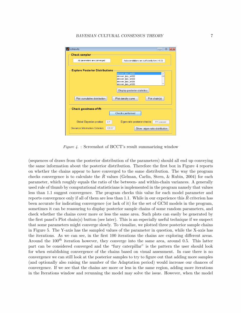
Figure 4 displays the window which pops up after the sampling is finished, except that initiallythe lower panel would be empty until the user pushes the Perform checks button (which here isalready changed to Checks performed).

(7) The upper panel (Check sampler) provides us with some basic information about the qualityof our posterior samples. The goal of this is to make sure that the sampler is accurately trackingthe correct posterior distribution on which the inferences are drawn. The first standard thatneeds to be met by the MCMC sampler is that the entire parameter space must be sufficientlyexplored. For that, sampling schemes should start multiple times, each with different startingvalues in different regions of the space of possible parameter values, and the generated sample chains


Figure 4. : Screenshot of BCCT’s result summarizing window

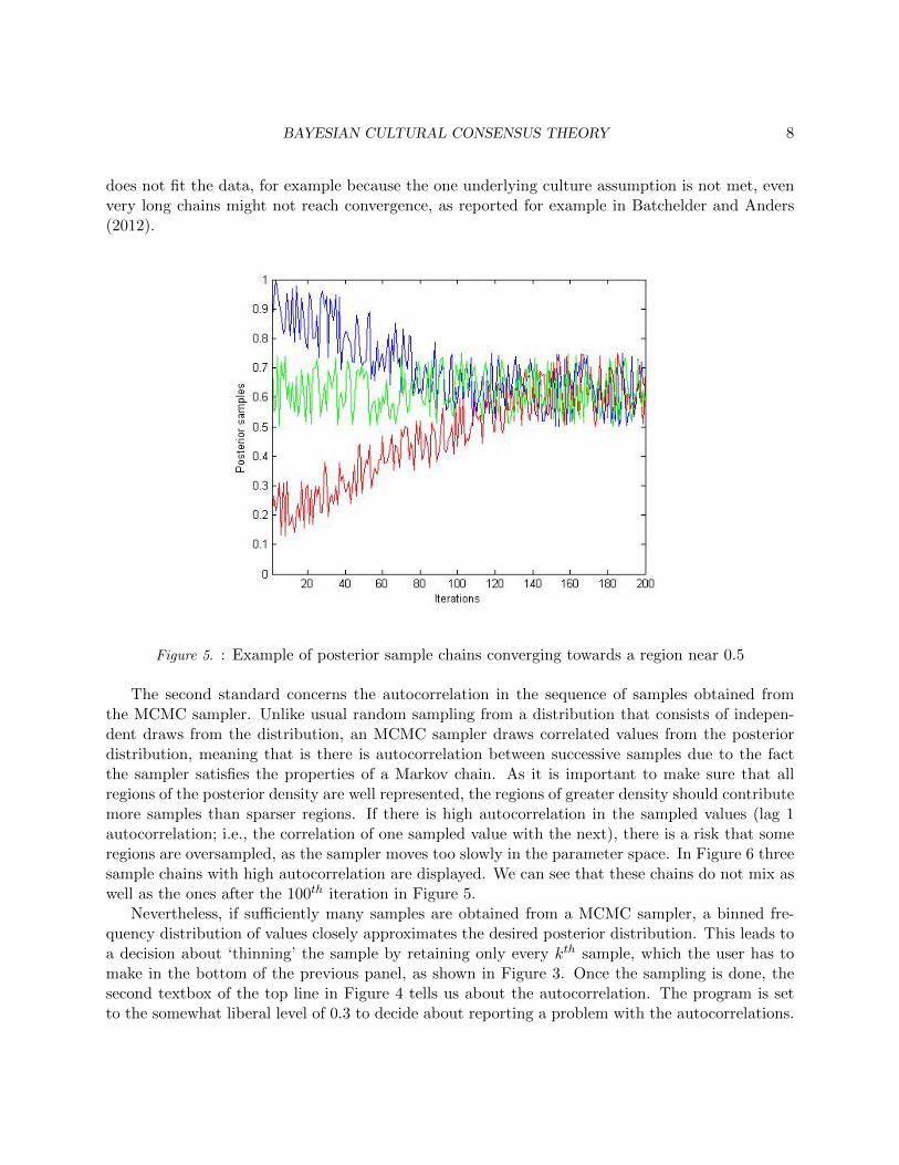
(sequences of draws from the posterior distribution of the parameters) should all end up conveyingthe same information about the posterior distribution. Therefore the first box in Figure 4 reportson whether the chains appear to have converged to the same distribution. The way the programchecks convergence is to calculate the R̂ values (Gelman, Carlin, Stern, & Rubin, 2004) for eachparameter, which roughly equals the ratio of the between- and within-chain variances. A generallyused rule of thumb by computational statisticians is implemented in the program namely that valuesless than 1.1 suggest convergence. The program checks this value for each model parameter andreports convergence only if all of them are less than 1.1. While in our experience this R̂ criterion hasbeen accurate for indicating convergence (or lack of it) for the set of GCM models in the program,sometimes it can be reassuring to display posterior sample chains of some random parameters, andcheck whether the chains cover more or less the same area. Such plots can easily be generated bythe first panel’s Plot chain(s) button (see later). This is an especially useful technique if we suspectthat some parameters might converge slowly. To visualize, we plotted three posterior sample chainsin Figure 5. The Y-axis has the sampled values of the parameter in question, while the X-axis hasthe iterations. As we can see, in the first 100 iterations the chains are exploring different areas.Around the 100th iteration however, they converge into the same area, around 0.5. This latterpart can be considered converged and the “fury caterpillar” is the pattern the user should lookfor when establishing convergence of the chains based on visual assessment. In case there is noconvergence we can still look at the posterior samples to try to figure out that adding more samples(and optionally also raising the number of the Adaptation period) would increase our chances ofconvergence. If we see that the chains are more or less in the same region, adding more iterationsin the Iterations window and rerunning the model may solve the issue. However, when the model


does not fit the data, for example because the one underlying culture assumption is not met, evenvery long chains might not reach convergence, as reported for example in Batchelder and Anders(2012).

Figure 5. : Example of posterior sample chains converging towards a region near 0.5

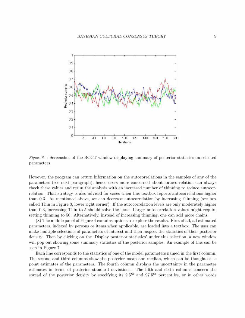
The second standard concerns the autocorrelation in the sequence of samples obtained fromthe MCMC sampler. Unlike usual random sampling from a distribution that consists of indepen-dent draws from the distribution, an MCMC sampler draws correlated values from the posteriordistribution, meaning that is there is autocorrelation between successive samples due to the factthe sampler satisfies the properties of a Markov chain. As it is important to make sure that allregions of the posterior density are well represented, the regions of greater density should contributemore samples than sparser regions. If there is high autocorrelation in the sampled values (lag 1autocorrelation; i.e., the correlation of one sampled value with the next), there is a risk that someregions are oversampled, as the sampler moves too slowly in the parameter space. In Figure 6 threesample chains with high autocorrelation are displayed. We can see that these chains do not mix aswell as the ones after the 100th iteration in Figure 5.

Nevertheless, if sufficiently many samples are obtained from a MCMC sampler, a binned fre-quency distribution of values closely approximates the desired posterior distribution. This leads toa decision about ‘thinning’ the sample by retaining only every kth sample, which the user has tomake in the bottom of the previous panel, as shown in Figure 3. Once the sampling is done, thesecond textbox of the top line in Figure 4 tells us about the autocorrelation. The program is setto the somewhat liberal level of 0.3 to decide about reporting a problem with the autocorrelations.


Figure 6. : Screenshot of the BCCT window displaying summary of posterior statistics on selectedparameters

However, the program can return information on the autocorrelations in the samples of any of theparameters (see next paragraph), hence users more concerned about autocorrelation can alwayscheck these values and rerun the analysis with an increased number of thinning to reduce autocor-relation. That strategy is also advised for cases when this textbox reports autocorrelations higherthan 0.3. As mentioned above, we can decrease autocorrelation by increasing thinning (see boxcalled Thin in Figure 3, lower right corner). If the autocorrelation levels are only moderately higherthan 0.3, increasing Thin to 5 should solve the issue. Larger autocorrelation values might requiresetting thinning to 50. Alternatively, instead of increasing thinning, one can add more chains.

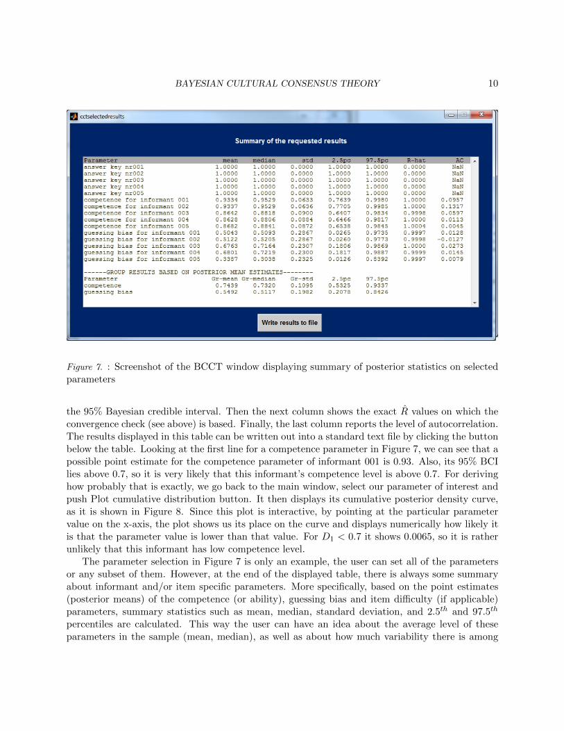
(8) The middle panel of Figure 4 contains options to explore the results. First of all, all estimatedparameters, indexed by persons or items when applicable, are loaded into a textbox. The user canmake multiple selections of parameters of interest and then inspect the statistics of their posteriordensity. Then by clicking on the ‘Display posterior statistics’ under this selection, a new windowwill pop out showing some summary statistics of the posterior samples. An example of this can beseen in Figure 7.

Each line corresponds to the statistics of one of the model parameters named in the first column.The second and third columns show the posterior mean and median, which can be thought of aspoint estimates of the parameters. The fourth column displays the uncertainty in the parameterestimates in terms of posterior standard deviations. The fifth and sixth columns concern thespread of the posterior density by specifying its 2.5th and 97.5th percentiles, or in other words


Figure 7. : Screenshot of the BCCT window displaying summary of posterior statistics on selectedparameters

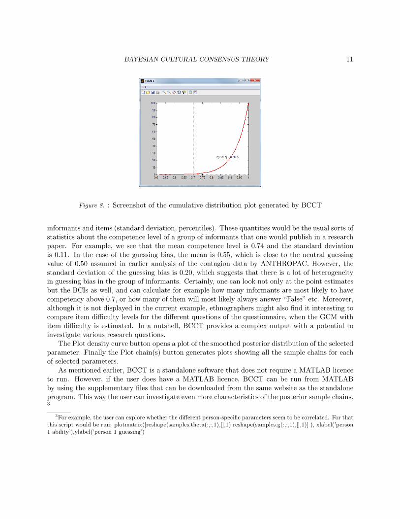
the 95% Bayesian credible interval. Then the next column shows the exact R̂ values on which theconvergence check (see above) is based. Finally, the last column reports the level of autocorrelation.The results displayed in this table can be written out into a standard text file by clicking the buttonbelow the table. Looking at the first line for a competence parameter in Figure 7, we can see that apossible point estimate for the competence parameter of informant 001 is 0.93. Also, its 95% BCIlies above 0.7, so it is very likely that this informant’s competence level is above 0.7. For derivinghow probably that is exactly, we go back to the main window, select our parameter of interest andpush Plot cumulative distribution button. It then displays its cumulative posterior density curve,as it is shown in Figure 8. Since this plot is interactive, by pointing at the particular parametervalue on the x-axis, the plot shows us its place on the curve and displays numerically how likely itis that the parameter value is lower than that value. For D1 < 0.7 it shows 0.0065, so it is ratherunlikely that this informant has low competence level.

The parameter selection in Figure 7 is only an example, the user can set all of the parametersor any subset of them. However, at the end of the displayed table, there is always some summaryabout informant and/or item specific parameters. More specifically, based on the point estimates(posterior means) of the competence (or ability), guessing bias and item difficulty (if applicable)parameters, summary statistics such as mean, median, standard deviation, and 2.5th and 97.5th

percentiles are calculated. This way the user can have an idea about the average level of theseparameters in the sample (mean, median), as well as about how much variability there is among


Figure 8. : Screenshot of the cumulative distribution plot generated by BCCT

informants and items (standard deviation, percentiles). These quantities would be the usual sorts ofstatistics about the competence level of a group of informants that one would publish in a researchpaper. For example, we see that the mean competence level is 0.74 and the standard deviationis 0.11. In the case of the guessing bias, the mean is 0.55, which is close to the neutral guessingvalue of 0.50 assumed in earlier analysis of the contagion data by ANTHROPAC. However, thestandard deviation of the guessing bias is 0.20, which suggests that there is a lot of heterogeneityin guessing bias in the group of informants. Certainly, one can look not only at the point estimatesbut the BCIs as well, and can calculate for example how many informants are most likely to havecompetency above 0.7, or how many of them will most likely always answer “False” etc. Moreover,although it is not displayed in the current example, ethnographers might also find it interesting tocompare item difficulty levels for the different questions of the questionnaire, when the GCM withitem difficulty is estimated. In a nutshell, BCCT provides a complex output with a potential toinvestigate various research questions.

The Plot density curve button opens a plot of the smoothed posterior distribution of the selectedparameter. Finally the Plot chain(s) button generates plots showing all the sample chains for eachof selected parameters.

As mentioned earlier, BCCT is a standalone software that does not require a MATLAB licenceto run. However, if the user does have a MATLAB licence, BCCT can be run from MATLABby using the supplementary files that can be downloaded from the same website as the standaloneprogram. This way the user can investigate even more characteristics of the posterior sample chains.3

3For example, the user can explore whether the different person-specific parameters seem to be correlated. For thatthis script would be run: plotmatrix([reshape(samples.theta(:,:,1),[],1) reshape(samples.g(:,:,1),[],1)] ), xlabel(’person1 ability’),ylabel(’person 1 guessing’)


Checking model fit

The Perform check button of the lower panel (already pushed in Figure 4) carries out severalgoodness-of-fit tests. As the tests may take a few minutes, this option is not executed automatically,but only at the user’s request. The lower panel of Figure 4 shows the results of these checks forthe example dataset.

Bayesian p-value. The posterior p-value reported in that box represents a global fit statisticof the current CCT model to the data. Calculation of this value is based on Bernoulli deviancefunctions (Karabatsos & Batchelder, 2003) of the raw data and replicated datasets based on theposterior distributions of the model parameters (set by a maximum 1000 samples in BCCT). Asthis statistic summarizes how likely it is that the current data, or data that are more extreme,would occur under the assumption that the model is correct, low p-values (under 0.05) indicate apoor fit.

Posterior predictive check of the one underlying culture assumption. The usual rule of thumbused by ethnographers (Weller, 2007) for supporting the single culture assumption is that this ratioof the first and the second eigenvalues is above 3. This rule is actually problematic, as the ratiois very dependent on the overall level of competence on the group of informants. The posteriorpredictive check option for the single culture assumption in the BCCT software improves upon theclassical eigenvalue test based on the recent work of Batchelder and Anders (2012). With BCCT wecan investigate the posterior predictive distribution of the ratio of the first to second eigenvalues ofseveral simulated datasets based on the posterior samples of model parameters. Then we can checkwhether the data eigenvalue ratio is within the 95% posterior predictive distribution of the modelbased eigenvalue ratios. If not, BCCT returns an error message saying: ‘PPC failed’, otherwise itreturns ‘PPC passed’. By pushing the button under the statistic we can see the smoothed posteriorpredictive distribution of these eigenvalues with the data’s eigenvalue ratio represented by a straightline, and this plot enables the user to exactly where the data eigenvalue ratio is with respect to thedistribution of simulated values.

Model selection with Deviance Information Criterion. An experienced user might analyze thesame dataset with several different GCM models which all pass the single culture posterior pre-dictive assumption as well as the Bayesian p-value indicates a reasonable model fit. Then the re-searcher is faced with the question of which model should they base their final conclusions. Whilethe Bayesian p-value and the eigen-ratio test provide goodness-of-fit tests in the absolute sense (themodel either fits or does not), with the Deviance Information Criterion (DIC; Spiegelhalter, Best,Carlin, & van der Linde, 2002) one can evaluate the relative goodness of fit of different models.DIC takes into account two important features of the model: the complexity (based on the numberof parameters) and the fit (measured by a deviance statistic). Naturally, more complex modelsfit better, therefore DIC penalizes based on the effective number of parameters in the model toarrive to a fair measure of fit. The model with the lowest DIC is supposed to be the best fittingone. For further discussion of DIC in the context of CCT modeling please consult Karabatsos andBatchelder (2003).


Model selection in general. Besides DIC, one can also consider more substantive argumentswhen it comes to model selection. Let us consider first the case of whether or not one shouldintroduce heterogeneity in the competence parameter. Cultural Consensus Theory was generallybased on the assumption that different people have different level of cultural knowledge. There-fore we recommend always keeping this parameter heterogenous. In theory however, such a modelconstraint might be useful when dealing with a group of cultural experts, or informants that areotherwise very homogeneous in their competence. Also it was this homogenous competence con-straint that allowed Batchelder and Romney (1988, Table 5) to construct conservative power tablesof the minimum number of informants needed to achieve pre-specified levels of confidence in theaccuracy of the estimated answer key.4

In CCT applications the guessing bias parameter has been fixed to a neutral level of g = 0.50for all respondents in order to be able to fit the data in ANTHROPAC or UCINET. While this maybe a good approximation, in signal detection studies (Macmillan & Creelman, 2005) the guessingbias found in data fits is not at a neutral level. For example, one can imagine situations wheresizable differences in guessing bias are to be expected (e.g., individual differences in how a personresponds when they do not know something or aspects of the wording of the particular items), inwhich case the assumption of homogeneity in this parameter might be untenable.

Finally, researchers might have constructed a survey with items of varying difficulty, in whichcase it is appropriate to allow for item heterogeneity in the model.

Saving results

(10) Finally results on the model parameters can be saved from the Summary of the requestedresults window as shown in Figure 7 by clicking the Write results to file button. This will resultin an excel file with its first sheet the posterior statistics on the selected parameters and with itssecond sheet the group results.

Testing BCCT

Here we provide a simulation study to demonstrate the parameter recovery accuracy of BCCT. Ahundred datasets – 25 informants and 50 items each – were generated based on the all heterogeneousmodel. ‘True’ parameter values were drawn from a uniform distribution between 0.1 and 0.99 forthe ability, guessing bias and item difficulty parameters. The answer key was sampled from aBernoulli distribution with probability 0.5. In the BCCT window the competence, guessing biasand item difficulty were set to “heterogeneous”. We checked convergence and autocorrelation ineach analysis and they met our standards defined above.

To evaluate the parameter recovery in the simulation study, two measures were calculated basedon the posterior samples of each run. First, we checked whether the 95% posterior BCIs of theestimates of abilities, guessing biases and item difficulties contained the simulated ‘true’ parametervalues. We calculated the proportion of times when it was outside of this region over persons (forability and guessing bias) and items (item difficulty) for each run. The first row of Table 1 showsthese percentages averaged over the 100 runs. Second, we calculated average absolute deviation(AAD) between simulated and estimated values. That is to say that that we took a posterior mean

4Right now such power tables can be constructed with BCCT in a timely manner only if BCCT is run from script.


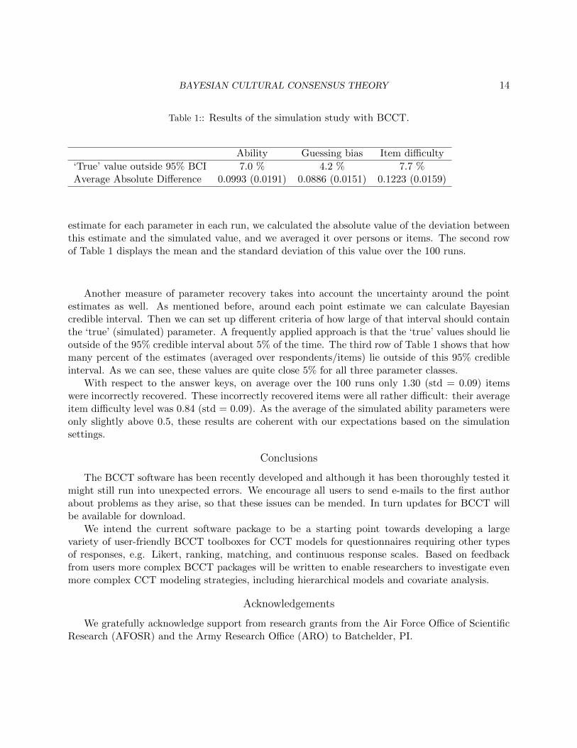
Table 1:: Results of the simulation study with BCCT.

Ability Guessing bias Item difficulty

‘True’ value outside 95% BCI 7.0 % 4.2 % 7.7 %Average Absolute Difference 0.0993 (0.0191) 0.0886 (0.0151) 0.1223 (0.0159)

estimate for each parameter in each run, we calculated the absolute value of the deviation betweenthis estimate and the simulated value, and we averaged it over persons or items. The second rowof Table 1 displays the mean and the standard deviation of this value over the 100 runs.

Another measure of parameter recovery takes into account the uncertainty around the pointestimates as well. As mentioned before, around each point estimate we can calculate Bayesiancredible interval. Then we can set up different criteria of how large of that interval should containthe ‘true’ (simulated) parameter. A frequently applied approach is that the ‘true’ values should lieoutside of the 95% credible interval about 5% of the time. The third row of Table 1 shows that howmany percent of the estimates (averaged over respondents/items) lie outside of this 95% credibleinterval. As we can see, these values are quite close 5% for all three parameter classes.

With respect to the answer keys, on average over the 100 runs only 1.30 (std = 0.09) itemswere incorrectly recovered. These incorrectly recovered items were all rather difficult: their averageitem difficulty level was 0.84 (std = 0.09). As the average of the simulated ability parameters wereonly slightly above 0.5, these results are coherent with our expectations based on the simulationsettings.

Conclusions

The BCCT software has been recently developed and although it has been thoroughly tested itmight still run into unexpected errors. We encourage all users to send e-mails to the first authorabout problems as they arise, so that these issues can be mended. In turn updates for BCCT willbe available for download.

We intend the current software package to be a starting point towards developing a largevariety of user-friendly BCCT toolboxes for CCT models for questionnaires requiring other typesof responses, e.g. Likert, ranking, matching, and continuous response scales. Based on feedbackfrom users more complex BCCT packages will be written to enable researchers to investigate evenmore complex CCT modeling strategies, including hierarchical models and covariate analysis.

Acknowledgements

We gratefully acknowledge support from research grants from the Air Force Office of ScientificResearch (AFOSR) and the Army Research Office (ARO) to Batchelder, PI.


References

Batchelder, W. H., & Anders, R. (2012). Cultural consensus theory: Comparing different concepts of culturaltruth. Journal of Mathematical Psychology . (in press)

Batchelder, W. H., & Romney, A. K. (1988). Test theory without an answer key. Psychometrika, 53 , 71-92.Borgatti, S. P. (1996). Anthropac 4.0. Natick, MA: Analytic Technologies.Borgatti, S. P., Everett, M. G., & Freeman, L. C. (2002). UCINET for Windows: Software for social network

analysis. Harvard, MA: Analytic Technologies.Gamerman, D., & Lopes, H. F. (2006). Markov chain Monte Carlo: Stochastic simulation for Bayesian

inference (2nd ed.). Boca Raton, FL: Chapman & Hall/CRC.Gelman, A., Carlin, J., Stern, H., & Rubin, D. (2004). Bayesian data analysis. New York: Chapman &

Hall.Hruschka, D. J., Sibley, L. M., Kalim, N., & Edmonds, J. K. (2008). When there is more than one answer key:

Cultural theories of postpartum hemorrhage in Matlab, Bangladesh. Field Methods, 20(4), 315–327.Karabatsos, G., & Batchelder, W. H. (2003). Markov chain estimation methods for test theory without an

answer key. Psychometrika, 68 , 373-389.Macmillan, N. A., & Creelman, C. D. (2005). Detection theory: A users guide (second ed.). Mahwah, N.J.:

Erlbaum.Plummer, M. (2011). Rjags: Bayesian graphic models using MCMC. (R package version 2.2.0-3

(http://CRAN.R-project.org/package=rjags))Robert, C. P., & Casella, G. (2004). Monte Carlo statistical methods. New York: Springer.Romney, A. K. (1999). Cultural consensus as a statistical model. Current Anthropology , 40 , 103-115.Romney, A. K., Weller, S. C., & Batchelder, W. H. (1986). Culture as Consensus: A theory of culture and

informant accuracy. American Anthropologist , 88 , 313-338.Spiegelhalter, D. J., Best, N. G., Carlin, B. P., & van der Linde, A. (2002). Bayesian measures of model

complexity and fit (with discussion). Journal of the Royal Statistical Society, Series B , 6 , 583–640.Weller, S. C. (1984). Cross-cultural concept of illness: Variation and validation. American Anthropologist ,

86 , 341-351.Weller, S. C. (2007). Cultural consensus theory: Applications and frequently asked questions. Field Methods,

19 , 339-368.

User’s guide to Bayesian Cultural Consensus Toolboxzoravecz/bayes/data/Articles/Users guide...

Documents

Transcript of User’s guide to Bayesian Cultural Consensus Toolboxzoravecz/bayes/data/Articles/Users guide...