
USER’S GUIDE FOR WATER9 SOFTWARE · USER’S GUIDE FOR WATER9 SOFTWARE Version 2.0.0 ... WATER9...
189
USER’S GUIDE FOR WATER9 SOFTWARE Version 2.0.0 August 16, 2001 Note that the updated version of this manual is available in a compiled help format that is available from WATER9. Office of Air Quality Planning and Standards U. S. Environmental Protection Agency Research Triangle Park, NC
Transcript of USER’S GUIDE FOR WATER9 SOFTWARE · USER’S GUIDE FOR WATER9 SOFTWARE Version 2.0.0 ... WATER9...

USER’S GUIDE FOR WATER9 SOFTWARE
Version 2.0.0
August 16, 2001
Note that the updated version of this manual is available in a compiled help format that is available from WATER9.
Office of Air Quality Planning and Standards U. S. Environmental Protection Agency
Research Triangle Park, NC

WATER9: Preface
ii
0. PREFACE Overview of WATER9 WATER9 is a Windows based computer program and consists of analytical expressions for estimating air emissions of individual waste constituents in wastewater collection, storage, treatment, and disposal facilities; a data base listing many of the organic compounds; and procedures for obtaining reports of constituent fates, including air emissions and treatment effectiveness. WATER9 is a significant upgrade of features previously obtained in the computer programs WATER8, Chem9, and Chemdat8. WATER9 contains a set of model units that can be used together in a project to provide a model for an entire facility. WATER9 is able to evaluate a full facility that contains multiple wastewater inlet streams, multiple collection systems, and complex treatment configurations. WATER9 provides separate emission estimates for each individual compound that is identified as a constituent of the wastes. The emission estimates are based upon the properties of the compound and its concentration in the wastes. To obtain these emission estimates, the user must identify the compounds of interest and provide their concentrations in the wastes. The identification of compounds can be made by selecting them from the data base that accompanies the program or by entering new information describing the properties of a compound not contained in the data base. WATER9 has the ability to use site-specific compound property information, and the ability to estimate missing compound property values. Estimates of the total air emissions from the wastes are obtained by summing the estimates for the individual compounds. WATER9 is used to estimate air emissions from site specific water treatment plants (including the prediction of biodegradation and sludge sorption of organics) for common wastewater treatment units including the following: drains, sumps, weirs, open drains, j traps, manhole covers, trenches, buried conduits (sewers), junction boxes, pump stations, clarifiers, trickling filters, aerated impoundments, quiescent impoundments, cooling towers, activated sludge units, storage tanks, wastewater separators, and settling ponds. WATER9 provides models for the evaluation of landfill, land treatment, and impoundment disposal facilities. The
WATER9: Preface
iii
collection system components of the modeling are currently based on theoretical models and correlations of data obtained by Enviromega (1993) and the University of Texas at Austin. WATER9 will be updated as additional investigations are available. WATER9 contains a compound property data base that has been updated with an extensive list of compound properties from the Design Institute for Physical Properties (DIPPR) 911 database. The Syracuse Research Corporation's SMILECAS Database is also included. This permits the WATER9 software to obtain compound structural information and CAS numbers for over 100,000 compounds. WATER9 will either accept user input of the compound properties used for the models or to automatically estimate the needed compound properties. WATER9 can adjust the compound properties on a unit basis, including the effects of temperature, multiphase partitioning, and pH.
Overview of this manual This WATER9 User’s Manual is provided in an Adobe Acrobat PDF format. There are several reasons for this that include the file size, the ability to print and read in many different types of computers, and the ability to search this manual using key words (click the binoculars icon). This user’s guide provides detailed information about the equations, calculation procedures, and methods for using WATER9, a graphical based computer program for estimating compound-specific air emissions from wastewater collection and treatment units. This preface contains advice for installing WATER9 and using the computer program. Preface 1: Installation of WATER9 WATER9 is designed to run under the Microsoft Windows graphical interface. WATER9 must be installed through the set-up program provided so that the location of Microsoft system files can be correctly identified in the file registry of Microsoft Windows. When you set-up WATER9, you will update the Windows/System with a set of system files (identified below). Once Windows locates these system files, you can run WATER9 under the following options. The following list indicates several options for using WATER9.

WATER9: Preface
iv
1. Download the WATER9 installation files from the EPA internet site. Save the
files in a temporary directory C:\temp. With the Windows Explorer in that temporary directory, run the WATER9 set-up program by double clicking on the set-up file icon with the mouse. Follow the instructions and install the program under the directory[C:\WATER9], in a directory named WATER9 on another drive, or using the setup defaults as a Program File[C:\Program files\Wastewater treatment models]. If the installation is successful, erase the files in the temporary directory. (You may wish to archive the compressed main installation file.)
2. Prepare a WATER9 removable disk (Zip or other disk) with the WATER9
files. You will run the program from your removable disk and project files may be saved to any folder that permits writing. This option will require that your computer system files are updated with Microsoft distribution files (provided through the download, or available separately). With this option, the WATER9 program may be upgraded by simply copying updated files to your removable disk.
3. Run the program from a WATER9 compact disk (CD). The CD will have
supporting files, manuals, and examples. You will run the program from your CD and files will be saved to your hard drive. With this option you will not be able to change the distribution data base files, which may be an advantage in some cases. You will be able to change the site specific compound property data base files. With this option, the program may be upgraded by simply changing to a different CD. The CD option requires that the Microsoft system files (listed below) are set-up in your Windows\System directory. In some Windows systems, WATER9 may be run directly from the WATER9 CD without the installation of Microsoft system files in the registry.
A WATER9 icon is associated with the WATER9 program and may be used as a shortcut on your Windows desktop, if you wish. Preface 2: Overview of Minimum Procedures (after set-up) For the user who only wishes to run a previously saved case study and estimate air
WATER9: Preface
v
emissions, the following minimum steps would provide an air emission estimate with a printed report. The user may follow the specific steps listed below to generate a sample report that is similar to the example given in Section 22. 1. Mouse click on the WATER9 icon on the Windows desktop to start WATER9.
Alternatively mouse click on start, programs, Wastewater Treatment Models (the default), then WATER9 to start the program. This assumes that the WATER9 program is installed on your computer.
2. Mouse click on Help Notes icon on the WATER9 main menu, then [minimum procedures] to open a help screen.
3. Follow the directions on the help screen. The help screen may be moved to one side by dragging the title bar of the help screen with a mouse.
4. The report that you generated will be visible on screen in a special display window. By pressing the appropriate button on the bottom right of the screen (with a mouse click) you may either (1) print the report on paper, (2) print the report to a computer file, or (3) print the data to a special formatted file that can be imported to Word or Excel (or other programs).
5. The use of WATER9 with a previously saved case study permits the user to generate a very large number of specialized reports for the saved case without the need to specify any additional information about the system. In addition the graphical interface permits the user to obtain detailed information about any of the units on screen by only placing the mouse pointer over the unit on the screen.
You may select another compound and print a report for the selected compound. You may click [Return] on the main menu to end this program. 6. To close the WATER9 session and return to the Windows desktop, mouse click
[Return] on the MAIN menu and then click [OK] to confirm the WATER9 program shut-down. WATER9 may also be minimized to temporarily remove the display (mouse click [_] on the WATER9 title bar).

WATER9: Preface
vi
You may use the minimum procedures to generate a new project from the beginning, or recover and modify the default file [manual.cwd] provided with the program for a new case study. When starting with a new file, you should restart the program and follow the procedures in GETTING STARTED with an initial screen as shown in Figure 1. If you are going to recover and modify the default file, follow the FILE menu procedures.
WATER9: Preface
vii
Help note: If you wish to learn more about using your mouse or the menus, it may be helpful to take a Windows tutorial provided by Microsoft.
Shortcuts for common operations (Hold [Ctrl] key down and press second key.) [Ctrl]C is add a compound to the project. A new selection window will appear. [Ctrl]P is to open a project file that is on disk. [Ctrl]S is to save your project that is already opened and edited to a set of files on your disk. You may use almost any name that you wish. [Ctrl]R is for a standard compound report for its path through each unit. [Ctrl]W is to edit the waste stream properties for all wastes. [Ctrl]E is for editing project compound properties. You select a compound. [Ctrl]L is for selecting a compound from your project list. These shortcuts may be especially useful to new users of WATER9 that find the large number of items in the main menu system to be confusing.

WATER9: Table of Contents
viii
0. PREFACE 2 OVERVIEW OF WATER9 2 OVERVIEW OF THIS MANUAL 3 PREFACE 1: INSTALLATION OF WATER9 3 PREFACE 2: OVERVIEW OF MINIMUM PROCEDURES (AFTER SET-UP) 4
1. INTRODUCTION 1-1
2. GETTING STARTED 2-1 STEP 1. LOAD AN EXISTING FILE 2-1 STEP 2. CALCULATE 2-2 STEP 3. EDIT WASTE STREAMS 2-2 STEP 4. EDIT UNIT PROPERTIES 2-2 STEP 5. RECALCULATE 2-3 STEP 6. VIEW RESULTS 2-3 OTHER CONSIDERATIONS 2-3 DEFAULT VALUES FOR UNIT PARAMETERS 2-4 USING WATER8 FILES 2-5
3. ACCESSING THE MAIN MENU 3-1 FILE 3-1
New Project 3-1 Load Project 3-1 Import Spreadsheet Files 3-1 Import WATER8 file 3-2 Save Project 3-2 Save as NaUTilus input file 3-2 Compress line set 3-2 Clear unit descriptions 3-2 Program file locations 3-2 Specify convergence parameters 3-3 Scan compound data base 3-3 Project information 3-3
VIEW 3-4 Overall summary 3-4 Emission summary II 3-4 Emission summary III 3-4 Emission summary IV 3-4 activated sludge summary 3-5 material balance 3-5 a compound unit summaries 3-5 compound summary at one unit 3-6 Scan list of compounds 3-6 All compound properties option 3-6 All compound data base options 3-7 Blank unit forms 3-8
WATER9: Table of Contents
ix
Print flow sheets 3-8 Save graphics file 3-8 Line waste flows 3-8 Line unit connections 3-9 Oil and solids in lines 3-9 Waste descriptions 3-9 Waste concentrations 3-9 Unit description forms 3-9 Detailed unit calculations 3-9 Compound property report 3-9 Waste loss in collection system 3-10 Flow and ventilation patterns 3-10 Nautilus output files 3-10 Compound fr, fm 3-10
SCREEN DISPLAY 3-11 Inlet and outlet units 3-11 Waste numbers 3-11 Oil and solids (g/s) 3-11 Oil and solids (ppmw) 3-12 Compound (ppmw) 3-12 Compound flow (g/s) 3-12 Fraction air loss 3-12 Ventilation 3-12 Vent parameters 3-13 Vent flows (g/s) 3-13 Vent concentrations 3-13 Mass transfer coef. 3-13 Water flow 3-13 Show emissions image 3-14 Show waste loading 3-14 Show unit numbers 3-14 Small unit icons 3-14
UNITS 3-15 Edit unit defaults 3-15 Edit general defaults 3-15 Global unit value sets 3-15 Global input buttons 3-15 Data quality check 3-15 Unit property edit 3-16 Delete a line 3-16 Add a line 3-16 Copy set of units to a unit 3-16 Reset defaults 3-16 Show default data base 3-17 Edit default data base 3-17 Storage tank vapor pressure 3-17 Process tank 3-17

WATER9: Table of Contents
x
Packed air 3-17 tank dispersion 3-17 Stripper 3-17
WASTE 3-18 Select compound in list 3-18 Edit waste set 3-18 Load new waste set 3-19 Add conventional sewer inlets to waste 3-19 import standard waste print file 3-19 Edit compound properties 3-19 Automatic compound properties 3-19 UNIFAC biorate correlation 3-20 Save list of compounds 3-21 Load new list of compounds 3-21 Add compounds to list 3-21
HELP NOTE PADS 3-21 minimum procedures 3-3 laying pipe 3-3 Exporting NaUTilus files 3-3 New case 3-3 Using screen displays 3-3 Hints and suggestions 3-3 Troubleshooting 3-3 Compound properties 3-3 Calculations 3-4 Examples 3-4 User notes 3-4
4. NEW PROJECT FILES 4-1 INITIAL SETUP 4-1 SELECTING COMPOUNDS 4-1 SELECTING WASTE CHARACTERISTICS 4-1 SELECTING TYPE OF UNITS 4-2 LAYING PIPE 4-2 EDITING THE PROPERTIES OF A UNIT 4-3 GENERAL INFORMATION 4-3 WASTE DISCHARGES 4-4 CALCULATIONS 4-4
5. LAYING PIPE 5-1 HOW DO I DROP THE PIPE INTO PLACE? 5-1 HOW DO I TRANSFER THE FLOW FROM A STREAM TO A UNIT ON A DIFFERENT SCREEN? 5-2 HOW DO I EDIT MY PIPE DEFINITIONS? 5-2 HOW DO I REMOVE A UNIT FROM MY WORKSHEET? 5-3 HOW DO I ADD ANOTHER UNIT TO MY WORKSHEET? 5-3 HOW DO I RECYCLE WASTE FLOWS? 5-3 HOW DO I ADD A VENT LINE TO MY SYSTEM? 5-4

WATER9: Table of Contents
xi
6. SELECTING COMPOUNDS FROM DATA BASE 6-1 SELECTION FORM 6-1 SEARCH UTILITIES 6-1 COMPOUND PROPERTY REVIEW 6-1 SMILES DATA BASE 6-1 TRANSFERRING THE COMPOUND LIST TO YOUR PROJECT 6-2 SAVING THE COMPOUND LIST 6-2 COMPOUND LISTS ASSOCIATED WITH PROJECT FILES 6-2
7. EDITING COMPOUND PROPERTIES 7-1 EDIT FORM 7-1 ACTIVE EDITING HELP 7-1 COMPOUND FRAGMENT EDITING 7-1
8. EDITING WASTE PROPERTIES 8-1 WASTE EDIT FORM 8-1 WASTE CHARACTERISTICS 8-1
Adding new compounds 8-2 Duplicate compounds 8-2 Deleting compounds 8-2
9. IMPORTING WASTEWATER SPREADSHEETS 9-1 STANDARD WASTE PRINT FILE FORMAT 9-1 CREATING A STANDARD WASTE PRINT FILE 9-2 IMPORTING AND VERIFICATION 9-2
10. CONTROL BUTTONS 10-1 DRAW MODE BUTTON 10-1
Toggle: draw mode 10-1 Toggle: lines off 10-1 Toggle: move lines 10-1
CALCULATION BUTTON 10-2 DIVERT FROM UNIT BUTTON 10-2 DIVERT TO WASTE BUTTON 10-2 DIVERT FLOW BUTTON 10-3 CONNECT BUTTON 10-3 SHEET SELECTION BUTTONS 10-4 COMPOUND NAME BOX 10-4 UNIT LIST BUTTON 10-4 STRAIGHTEN BUTTON 10-5
11. IMPORTING WATER8 FILES 11-5 POTENTIAL CONCERNS 11-5 ENHANCEMENTS IN WATER9 11-2 HOW DO I IMPORT WATER8 FILES? 11-2 EDITING YOUR WORK AND VERIFICATION 11-3
WATER9: Table of Contents
xii
12. NAUTILUS COMPATABILITY 12-1
13. UNIT NUMBERS AND DESCRIPTIONS 13-1 UNIT 1. OPEN TRENCH 13-1
sludge dewatering 13-1 UNIT 2. CLOSED TRENCH 13-1 UNIT 3. OPEN HUB 13-1 UNIT 4. COVERED DRAIN 13-1 UNIT 5. MANHOLE COVER 13-1 UNIT 6. RESERVED 13-1 UNIT 7. OPEN SUMP 13-2 UNIT 8. CLOSED SUMP, VENT 13-2 UNIT 9. RESERVED 13-2 UNIT 10. OPENING IN CONDUIT 13-2 UNIT 11. OPEN J DRAIN 13-2 UNIT 12. HEADSPACE SEALED 13-2 UNIT 13. WEIR, WATERFALL 13-3 UNIT 14. HARD PIPED, NO HEADSPACE 13-3 UNIT 15. LIFT OR PUMP STATION 13-3
open sumps with pumping 13-3 UNIT 16. VENT CONDUIT 13-3 UNIT 17. WATER SCRUBBER 13-3 UNIT 18. CONDENSER 13-3 UNIT 19. CONTINUOUS STEAM STRIPPER 13-4 UNIT 20. CONTROL DEVICE 13-4 UNIT 21. BAR SCREEN 13-4 UNIT 22. DAF OR GRIT SEPARATION 13-4 UNIT 23. RESERVED 13-4 UNIT 24. MIX TANK 13-4 UNIT 25. PRIMARY MUNICIPAL CLARIFIER 13-5
rectangular clarifier and double weirs 13-5 UNIT 26. EQUALIZATION 13-5
equalization pond, plug flow 13-5 UNIT 27. TRICKLING FILTER 13-6
cooling tower with biological activity 13-6 UNIT 28. AERATED BIOTREATMENT 13-6 UNIT 29. ACTIVATED SLUDGE BIOTREATMENT 13-7 UNIT 30. DIFFUSED AIR BIOTREATMENT 13-8
UNOX and closed vented system biotreatment 13-8 UNIT 31. COOLING TOWER 13-8 UNIT 32. CIRCULAR CLARIFIER 13-8 UNIT 33. API SEPARATOR OR OIL WATER SEPARATOR 13-9 UNIT 34. STORAGE TANK 13-9
34 A. fixed roof tank model. 13-9 34 B. open roof tank model. 13-10 34 C. constant level fixed roof tank model. 13-10

WATER9: Table of Contents
xiii
34 D. open roof agitated tank. 13-10 34 E. submerged aeration tank. 13-10
UNIT 35. OIL FILM UNIT 13-11 oil press separator 13-11
UNIT 36. LAGOON 13-11 UNIT 37. BIOFILTER 13-11 UNIT 38. RESERVED 13-11 UNIT 39. COVERED SEPARATOR 13-11 UNIT 40. RECTANGULAR COVERED CLARIFIER. 13-11 UNIT 41. RESERVED 13-12 UNIT 42. RESERVED 13-12 UNIT 43. LANDFILL 13-12 UNIT 44. POROUS SOLIDS UNIT 13-12 UNIT 45. LAND TREATMENT 13-12 UNIT 46. SYSTEM EXIT STREAM 13-12 UNIT 47. DIVERT FLOW 13-13 UNIT 48. OIL REMOVAL STREAM 13-13 UNIT 49. SOLIDS REMOVAL STREAM 13-13
14. DEFINITIONS 14-1 DISCUSSION OF COLLECTION SYSTEM ELEMENTS 14-1 DEFINITION OF TERMS 14-1
15. TROUBLESHOOTING PROCEDURES 15-1 PROBLEMS AND SOLUTIONS 15-1
16. UNIFAC CALCULATIONS 16-1 BACKGROUND TO UNIFAC 16-1 ADVANTAGES OF THE UNIFAC METHOD 16-1 LIMITATIONS OF THE UNIFAC METHOD 16-2 THERMODYNAMICS OF PHASE SEPARATION 16-2 THERMODYNAMICS OF PHASE PARTITIONING 16-3 ACTIVITY IN VO TEST METHOD MATERIALS 16-3 REFERENCES 16-4
17. MISSING COMPOUND PROPERTY ESTIMATION 17-1 OVERVIEW OF THE ORDER OF ESTIMATION 17-1 EQUATIONS FOR DETERMINING COMPOUND PROPERTIES 17-2
First-Order Biorate Constant 17-2 Henry’s Law Constant 17-2 Solubility 17-2 Octanol-Water Partition Coefficient 17-2 Diffusion Coefficients 17-4
18. SMILES DATA BASE 18-1
19. ADDING A COMPOUND AND PROPERTIES 19-1
WATER9: Table of Contents
xiv
20. VERIFYING AUTOMATIC PROPERTY ESTIMATION 20-1
21. EXAMPLE OF PRINTING A REPORT 21-1
22. EXAMPLE OF A PRINTED REPORT 22-1
23. SOURCE CODE 23-1
24. COLLECTION SYSTEM EXAMPLE 24-1
25. SAMPLE CALCULATIONS 25-1 STORAGE TANK 25-1 OPEN TRENCH 25-2
Owens Model 25-3 Parkhurst and Pomeroy Model 25-4 Mackay Liquid Mass Transfer Model 25-5
WATER9: Introduction
1-1
1. INTRODUCTION
The Wastewater and Treatment Emissions Routines (or WATER9) consists of the following features: 1. analytical expressions for estimating air emissions of individual waste
constituents in wastewater collection and treatment units, 2. a graphical interface that corresponds to engineering flow diagrams, 3. a data base listing many of the common organic compounds and their
properties, 4. methods to automatically estimate missing compound properties, 5. methods to import site information from spreadsheets, 6. extensive list of options for viewing and printing reports, 7. flexibility in specifying recycle water, sludges, oils, and vents, 8. help note pads for obtaining printouts of emission estimates and
using the program, and 9. overall air emissions from a site (collection and treatment units). In the WATER9 program, separate emission estimates are made for each individual compound identified as a constituent of the waste. The emission estimates are based on the properties of the compound, its concentration in the wastes, and the path of the waste through the collection and treatment system. To obtain emission estimates, the user must identify the compounds of interest and provide their concentrations in the waste. The identification of compounds can be made by selecting them from the data base that accompanies the program or by entering new information describing the properties of a compound not contained in the data base. Estimates of total emissions from a waste are obtained by summing the estimates for the individual compounds. The report “Air Emission Models for Waste and Wastewater”1, especially
1 For further information, see Air Emissions Models for Waste and Wastewater, U.S. Environmental Protection Agency, Office of Air Quality Planning and Standards, Research Triangle Park, NC, November 1994, EPA-453/R-94-080A.

WATER9: Introduction
1-2
Appendices A and C and Chapters 4, 5, and 6, provides detailed information related to compound properties and air emission models. The WATER9 program is based on and provides compound data organized in file structures compatible with the requirements of WATER8, CHEM9, and CHEMDAT8, which is the data base described in that document.
This guide offers details of the equipment and skills needed to run the WATER9 program, instructions on getting started, and a run-through of each procedure in the program. Section 16 offers a technical explanation of the UNIFAC method of estimating compound property values; Section 17 describes how to make automatic property calculations. Section 18 gives an example of a procedure for adding a compound to the data base with supporting UNIFAC parameters; Sections 19 and 20 provides an example of the procedures for using “Check Data.” Sections 21 and 22 contain examples of a procedure for printing a report and an example of a printed report, respectively. Section 23 shows the source code used in the calculations for the units. Moreover Sections 24 and 25 present sample calculations for those wastewater units not included in the report “Air Emission Models...” .

WATER9: Introduction
1-3
The WATER9 program, through a series of HELP screens and messages, allows you to:
1. Have access to over 2000 compounds and their compound-specific data from the master list of chemicals.
2. Identify up to 100 selected compounds from the master list of
chemicals for a specific project. 3. Estimate the value of compound properties that are not available in
the data base. 4. Specify the operating parameters of the wastewater collection system
and treatment facility, together with site-specific compound properties (a project).
5. Predict the compound-specific short-term and long-term air emission
rates from the facility. 6. Print a report of emission estimates. 7. Save and retrieve individual projects in separate computer files. 8. Save site specific compound data that is associated with individual
projects in separate computer files. (especially site specific biorates) 9. Load site specific compound data and waste stream information that
is associated with an individual project (1) into another project (2). This permits evaluation of a waste set in alternative treatment systems.

WATER9: Introduction
1-4
The WATER9 program and supporting data base files are available as a download from the Internet or are available in a set of installation files. The installation files are small enough to be distributed as a set of 1.44M 3.5 inch floppies. WATER9 was designed to run on a Pentium PC with at least 16M RAM. Multimedia and high resolution screens are helpful. A 386 machine with Windows and 4M RAM is probably minimum, but WATER9 will run very slowly on minimum machines. The program can be run from your PC’s hard disk by first installing the program in your computer. A color monitor is required. The program is written for a Microsoft Windows operating system, which provides an interface to printers, and other system supports. To use the optional UNIFAC procedures, you will also need to have a basic understanding of compound structures from organic chemistry. References are provided in Section 16 to assist you in understanding the basis of the calculations with UNIFAC as well as the other procedures contained in the program. To assist you in matching the compound structures with the UNIFAC fragments, a graphical utility was written, and is automatically available when you edit the UNIFAC fragments. A large database of Smiles strings, CAS numbers, and compound names, together with a defragmenting utility will provide some assistance in extracting compound fragment data from additional compounds. There are three computer equipment options for using the WATER9 files: a high-capacity removable disk, a hard disk, or a CD drive. The following files are required to run the program: Windows bootstrap files (Microsoft)
VB6STKIT.DLL COMCAT.DLL MSVCRT40.DLL OLEPRO32.DLL STDOLE2.TLB ASYCFILT.DLL OLEAUT32.DLL msvbvm60.dll
Windows system files (Microsoft) grid32.ocx mfc40.dll anibtn32.ocx comdlg32.ocx gauge32.ocx keysta32.ocx spin32.ocx vb5db.dll msrepl35.dll msrd2x35.dll expsrv.dll vbajet32.dll

WATER9: Introduction
1-5
msjint35.dll msjter35.dll msjet35.dll dao350.dll rdocurs.dll msrdo20.dll mdac_typ.dll WATER9 program files WATER9.exe BIODATA.CH7 CMPPROP.CWP MASTER.CH7 DEFPROP.CWP HONFETOT.CH8 TRANSLAT.7 UNIFAC.CH7 COLLECT.CWP CMPREF.CWP ISCDATA.SET SMILESRIP.TXT MASTERTRI.CH7 AUTO*.* (10 files) SMILECAS.MDB FRAGMENTDATA.CH7 WATER9 project files (each name below has 5 supporting files) chapter 4 BACTLAER3 landfill wastepile a print example crossflow cooling tower example covered separators mixing in biotreatment example DCE spill example treatment plant 2 ISBL example treatment plant activated sludge municipal plant covered units POTW Trickling filter municipal plant front units covered WATER9 compound files (list of compounds) append8 HAP108 TRIset HAP WATER9 help files calc collection compound displays examples hints NaUTilus new pipe report tagg trouble user1 WATER8 WATER8 project files (for conversion to WATER9) BACTLAER cooltower EXHA3 EXHA4 EXHA5 EXHA11 EXHA12 EXHA22
WATER9: Introduction
1-6
DIRWTR9 (can direct the program to save or use files from another directory) README.1ST (information to use the program or program updates) Unit forms and documentation.xls (workbook to prepare spreadsheet information for WATER9 importing) NaUTilus files ISBL.CCC ISBL.EXE ISBL.FIN ISBL.IN ISBL.OUT ISBL.WWA ISBL.WWD ISBL.WWT ISBL.WWW OSBL.EXE OSBL.FIN OSBL.IN OSBL.OUT RUNNAUT.BAT
WATER9: GETTING STARTED
2-1
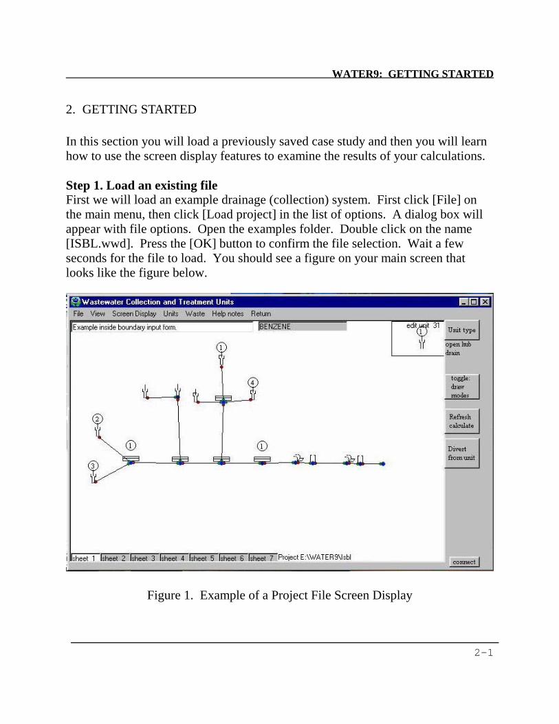
2. GETTING STARTED In this section you will load a previously saved case study and then you will learn how to use the screen display features to examine the results of your calculations. Step 1. Load an existing file First we will load an example drainage (collection) system. First click [File] on the main menu, then click [Load project] in the list of options. A dialog box will appear with file options. Open the examples folder. Double click on the name [ISBL.wwd]. Press the [OK] button to confirm the file selection. Wait a few seconds for the file to load. You should see a figure on your main screen that looks like the figure below.
Figure 1. Example of a Project File Screen Display

WATER9: GETTING STARTED
2-2
Step 2. Calculate Press the [refresh calculate] or [Update] button to calculate the performance of the system. You will note the progress of the iterative calculations by the filling of the progress bar in the center of the screen. You will see seven drains connected by sewer runs, followed by waterfalls and manholes. Step 3. Edit waste streams Note that waste is discharged into hubs that are indicated with circles with enclosed numbers in the circles. Those units are hubs that are receiving waste streams. To examine the hub under the circle containing the number 4, point the mouse arrow to the red dot under the hub on the WATER9 computer screen. An information box will appear under the unit informing you that the unit number is 15 and it discharges into unit 14 (to the left). Move the mouse pointer to the left to confirm the receiving unit number. The flow rate and calculated underflow wastewater depth is also displayed. Let's confirm the flow rate into unit 15. Click [Waste] on the main menu, then click [edit waste set] in the list of options (or use the shortcut [Ctrl]W). Under the column labeled waste 4 (remember the number in the circle?) you will see the flow rate of 0.0001 L/s. If you change the flow rate at this point in the collection system and then recalculate, a different flow rate will appear in the information box under unit 15 at the next time. Click on the button [return from waste edit] now. We are still interested in unit 15. First we will add the unit numbers to the display so that we can easily identify unit 15. Click [Screen Display] on the main menu, then click [show unit numbers] in the list of options. You will see the unit numbers downstream of the unit. Step 4. Edit unit properties We will examine the input properties of unit 15 now. Click on the red dot under the unit. An unit specific control panel will appear. Click on the button [Edit Properties] on the control panel. We will first check on the radius of the 4 inch ID drop pipe. Click on the number 5 in the input box to the right.

WATER9: GETTING STARTED
2-3
We know that it is a two-inch inside radius pipe. Press the conversion factors button at the top of the covered drain property form. A conversion utility will appear at the bottom of the form. Click on [in to cm] in the conversion factor list. Enter the number 2 in the box labeled text2. The number 5.08 appears on the right. Double click on the radius of drop pipe to insert this value. Press [OK] to use the edited values that are presented in this form. Step 5. Recalculate Press the [refresh] button to recalculate the performance of the system. Press the [refresh] button several times to improve the calculations (the number in the box, error, is smaller). Click [Screen Display] on the main menu, then click [show emissions image] in the list of options. You will see a shaded circle over the units that discharge headspace. Since WATER9 depends on successive calculations to account for recycle and countercurrent headspace flows in the collection system network, it is important to provide enough calculations iterations. Either manually press the refresh calculate button until the results converge, or change the number of iterations under [file] [convergence parameters] Step 6. View results In order to view the results of your calculations, now click on [Screen Display] on the main menu. Then click [fraction air loss]. As you point the mouse to individual units, the fraction air loss of those units are displayed in a yellow information box. Other considerations You may define a default set for each project. The set of default values will be automatically saved when each project is saved. To use one of the previously defined default set for a new project, first load the old project that contains the desired default set. Edit and save the project as a new project with the name of the new project. Place the mouse over the unit position. The unit position contains a larger blue dot, a red dot at the exit of the line, one or more green dots from inlet streams, and
WATER9: GETTING STARTED
2-4
a crude sketch of the unit over the unit position. The mouse icon will turn into a <-> symbol at the unit. Click to open the edit unit box. In an edit unit box, you may change the type of unit, change the unit properties, add waste streams to the unit, or in the case of flow diversion units, edit the flow diversion properties. The flow diversion properties are edited from the end of the line (green dot), not the beginning of the line (red dot). Please separate the units enough to avoid confusion. Move the units out of the way if you run into trouble. Sometimes you have multiple units with similar properties, either in series or parallel. You may save time by specifying the properties for a unit, then using the copy function in the edit unit box. Open the edit unit box for the next unit. and paste to transfer the saved properties to the next unit. The flow of wastewater can be transferred from units presented on one screen to those on another screen. When the mouse is moved across the end of a line, the divert flow button at the top of the screen is activated. Press that button. Enter the unit number of the unit that you wish to receive the flow. Then press the [OK] button. Default values for unit parameters Default values are provided for all parameters for each type of unit. Although these default values are believed to be reasonably applicable to many of the units present at wastewater collection and treatment sites, it is recognized that some sites can be characterized by different default values. A method is provided in WATER9 to permit changes to the default values before units are placed on the screen of WATER9. The new units will then have the changed default values that were previously specified. This will save time because the individual units will not have to be updated individually for the changed default values. Examples of updated default values include opening sizes at openings and the slope of the underground conduit. You may define a default set for each project. The set of default values will be automatically saved when each project is saved. To use one of the previously defined default set for a new project, first load the old project that contains the

WATER9: GETTING STARTED
2-5
desired default set. Edit and save the project as a new project with the name of the new project.
Using WATER8 files You can load a WATER8 file, and the program will automatically transfer the compound properties in the *.ccc WATER8 compound file into WATER9. Because WATER9 is very different from WATER8 in program structure, you may not save WATER9 information in a WATER8 format. You may delete the units definitions in WATER9 and retain the compound list for another project.
WATER9: MAIN MENU- FILES
3-1
3. ACCESSING THE MAIN MENU The MAIN menu is always active and available for use, unless calculations are in progress. The mouse may be used to select a menu item by clicking. When a menu item is selected, other menus or input screens may appear to assist you in performing some of the program options. The following sections describe some of the options provided through the main menu. File
New Project Use this option to erase the existing project and start a new project. A more conservative approach would be to shut down the program, thus erasing all WATER9 allocated memory and restarting. Restarting WATER9 would remove any potential conflict with previous projects.
Load Project Use this option to load an existing project that was saved as a set of project files. This option will overwrite any existing WATER9 project in computer memory. It will have no effect on previously saved projects.
Import Spreadsheet Files Use this option to load project information from a spreadsheet format into a WATER9 format. There are three options for importing spreadsheet data: unit data, compound data, and waste stream data. Each of these options has a different format. To obtain information about format requirements, load the Excel workbook “Unit form and documentation.xls”. The instructions are in the sheets of the workbook. Individual sheets are saved as tab separated txt files. WATER9 will automatically load and translate these txt files. The use of this option will require that you place the information in your existing spreadsheets in the special format of the workbook, “Unit form and documentation.xls”.

WATER9: MAIN MENU- FILES
3-2
Import WATER8 file Use this option to add a WATER8 file to your project. The WATER8 units will be added on the first blank screen. This operation will not erase the WATER9 project information. This option is described in more detail in a Section 11.
Save Project Use this option to save the existing project. A series of files will be saved. Different parts of the project are saved in different files. You will only need to identify one file name for Loading and saving because WATER9 automatically uses this file name for each of the other associated files.
Save as NaUTilus input file Use this option to translate your WATER9 project information to the NaUTilus program. This operation will have no effect on the WATER9 project information. This option is described in more detail in a separate Section 12.
Compress line set When WATER9 adds a new unit, the new unit number is greater than the other unit numbers. In the situation when some units have been deleted, some lower numbers may be available. This procedure uses all of the available lower unit numbers by reassigning unit numbers. This procedure can reduce the size of project files.
Clear unit descriptions Use this option to erase all the units in the project. You will retain your waste descriptions. This option is used to start over with the unit descriptions. You will be asked to confirm your intention to erase the units.
Program file locations Use this option to specify the directory for the program files and the project files. You should not normally change these values. If WATER9 has not identified the location of project files, it will automatically scan the drives to search for the WATER9 program location, starting with H:WATER9i, down to H:WATER9, and continuing to C:WATER9.
WATER9: MAIN MENU- FILES
3-3
Specify convergence parameters Warning: these parameters should not be reset unless you understand what you are doing or if there are serious convergence problems. 1. Number of iterations- The method that WATER9 uses to calculate network
performance is to calculate all elements in the network several times. The number of times that this occurs is specified as the number of interactions in the first input line.
2. Specify line vent rates- The default value is 0, or calculate the line vents. If the line vent rates are specified, then the value is set to 1, or, for WATER8 compatibility, the value is automatically set to 2.
3. Iterations in vent convergence- this value, combined with the number of passes determines the total iterations for calculating the line vent rates.
4. Allowable vent error- If the vent calculations produce less than the allowable vent error, additional iterations may be skipped.
5. Acceleration factor- This is an adjustable value used for setting bounds on the internal vent optimization procedures.
6. Change in pressure- This is a second adjustable value used for setting bounds on the internal vent optimization procedures. Smaller values produce more accurate results at the expense of calculation times.
Scan compound data base Use this option to generate a report for each compound in the data base. A typical report could contain the following: 1. compound name 2. Henry’s law for 100 °C 3. estimated Henry’s law for 100 °C 4. UNIFAC code for fragment information This option will not be available if the text in the option is gray.
Project information Use this option to specify descriptive text that will be saved with your project files.

WATER9: MAIN MENU- VIEW
3-4
View
Overall summary This option generates a summary report that may be viewed, printed, or saved as a file. The report contains the following: 1. header information 2. compound name 3. total compound emission rate (g/s) 4. fraction lost as air emissions 5. fraction removed by treatment 6. loading in the waste streams 7. overall compound material balance
Emission summary II This option generates a summary report that may be viewed, printed, or saved as a file. The report contains the following: 1. header information 2. compound name 3. total compound emission rate (g/s) 4. fraction lost as air emissions 5. total compound emission rate (lb/day) 6. loading in the waste stream (ppmw)
Emission summary III This option generates a summary report that may be viewed, printed, or saved as a file. The report contains the following: 1. header information 2. compound name 3. total compound emission rate (Mg/yr) 4. fraction lost in collection system 5. fraction lost in treatment system 6. fraction treated
Emission summary IV This option generates a summary report that may be viewed, printed, or saved as a file. The report contains the following:
WATER9: MAIN MENU- VIEW
3-5
1. header information 2. compound names for each compound in project 3. fraction controlled for each compound 4. fraction lost to the air for each compound 5. fraction remaining after treatment 6. fraction removal by treatment
activated sludge summary This option generates a summary report of biological treatment units only. The report may be viewed, printed, or saved as a file. The report contains the following: 1. header information 2. compound name 3. fraction lost to air 4. fraction remaining in unit effluent 5. fraction removed by biological treatment 6. hydraulic residence time information
material balance This option generates a series of material balances for the individual units and the overall system for the selected compound. The report that may be viewed, printed, or saved as a file. The report contains the following: 1. header information 2. compound sum in, out, and removal for water and headspace for each unit 3. compound sum in, out, and removal for each unit 4. overall compound mass balance 5. headspace vent flow material balance 6. headspace concentrations in each collection unit.
a compound unit summaries This option generates a summary report for the selected compound that may be viewed, printed, or saved as a file. The report contains the following: 1. header information 2. unit name 3. total compound loading at unit (g/s) 4. compound air emissions (g/s)
WATER9: MAIN MENU- VIEW
3-6
5. compound unit exit rate (g/s) 6. compound unit removal rate (g/s)
compound summary at one unit This option generates a summary report for each of the project compound at a selected unit that may be viewed, printed, or saved as a file. You must select a unit before using this option. (Click on the unit you want.)The report contains the following:
1. the name of compound. 2. the concentration in, 3. the fraction air lost in the unit, 4. the fraction removed (biodegraded) in the unit, and 5. the concentration leaving the unit.
Scan list of compounds This option generates a summary report for the fate of an external list of compounds in your project. WATER9 stores list of compounds as files with an extension of [.ccc]. You first have load a project file. Then you choose this option from the main menu. You then select a compound file (that can contain hundreds of compounds). The scan list report may be viewed, printed, or saved as a file. The report contains the following:
1. the CAS number, 2. the name of the compound, 3. the fraction air lost in the entire system, 4. the fraction removed (biodegraded) in the entire system, 5. the fraction sorbed in the entire system, and 6. the fraction exiting in the wastewater from the entire system.
All compound properties option
All compound emissions at selected unit A unit is selected by clicking the mouse on the base of the unit. A report is generated for each compound in the project at that unit.
WATER9: MAIN MENU- VIEW
3-7
All compound loading at selected unit A unit is selected by clicking the mouse on the base of the unit. A report is generated for the inlet concentration of each compound in the project that is present at that unit, both from waste addition at the unit and waste addition upstream of the unit.
All HAP compound list For each compound in the data base that is identified as a hazardous air pollutant, the compound name, CAS number, HL value, and the vapor pressure is listed.
All compound unit summaries For each compound in the project, a list of emissions is generated for each unit.
Selected compound structure For each compound in the project, a list of the number of fragments and the fragment number is generated.
Biorate estimation For each compound in the project, a list is generated of the number of fragments and the fragment number with the biorate factor and the overall estimated biorate.
Short list H, fm, fr A report is generated with Henry’s law values, the fraction measured with EPA Method 25D, and the fraction recovered in a design steam stripper for each of the compounds selected for the project.
All compound data base options
All compound H<.1,fe A report is generated with the fraction measured with EPA Method 25D, the fraction recovered in a design steam stripper, and the estimated air emission loss in a reference wastewater treatment system for each of the compounds in the master data base with a Henry’s law value less than 0.1 atm/mol fraction in water.
All compound HL estimation validation A report is generated with the estimated value of HL compared to the listed value

WATER9: MAIN MENU- VIEW
3-8
of HL in the data base. This report can be used to evaluate the expected accuracy and precision of the HL estimation procedure.
All compound fm, fr, fe A report is generated with the fraction measured with EPA Method 25D, the fraction recovered in a design steam stripper, and the estimated air emission loss in a reference wastewater treatment system for each of the compounds in the master data base.
All compound density, mwt A report is generated with the name of the compound, the density of the liquid pure compound, and the compound molecular weight.
All compound HL, CAS in data base A report is generated with the name of the compound and the Henry’s law value for each of the compounds in the master data base, together with the CAS number.
All compound HL A report is generated with the name of the compound, the presence of a UNIFAC code ("U" if present), and the Henry’s law value in two different units.
Blank unit forms Forms are printed to use as input sheets for unit characteristics.
Print flow sheets This option prints the on-screen images on your printer, together with some line information.
Save graphics file This option saves the on-screen image as a color bitmap image that may be used in reports. Save the image in a file with a descriptive name. The image may be edited with a several graphics editors. This graphics file is helpful when describing your system and may be included in reports generated by a word processor program (not provided).
Line waste flows This report provides a list of the waste flow rate in each line (unit) in the project.

WATER9: MAIN MENU- VIEW
3-9
This information is also available with the [screen display] options.
Line unit connections This report provides a list of each line in the project with the connections to other lines. This report may be inspected to verify that the unit connections are correctly specified.
Oil and solids in lines This report provides a listing of oil and solid concentrations in each line. The information in this report is available for viewing or printing.
Waste descriptions This report provides a listing of oil and solid concentrations in each waste stream, together with the temperature of the waste and the flow rate of the waste stream. The information in this report is available for viewing or printing.
Waste concentrations This report provides a listing of the concentrations of each selected compound in the first five specified wastes. The information for the entire waste set is available in spreadsheet format under [waste][edit waste set].
Unit description forms This report provides a listing of the project inputs for a limited number of units.
Detailed unit calculations This report provides an extensive amount of detail about the calculations for a compound in each unit. It is suggested that the information be viewed only if more than a few units are in your project. Printing to a file will enable you to print a portion of the report with a word processor. Individual unit reports are available with the view button on the unit pop-up menu.
Compound property report This report provides a listing of the compounds and their properties that are used in the calculations. This listing is for 25ºC, the properties are adjusted for the actual temperature for each unit.
WATER9: MAIN MENU- VIEW
3-10
Waste loss in collection system This report provides a listing of the source of air emissions for each unit, as well as the input flow rate (g/s) and the air emission loss (g/s). Update the calculations before viewing this report.
Flow and ventilation patterns This report provides a listing of the headspace flow rate, and vent rate for each unit, along with the unit name, and the type of unit.
Nautilus output files NaUTilus is a compiled computer program that was developed at the University of Texas at Austin. It is a Fortran based text interpreter program that estimates air emissions from collection systems based upon input files provided by the user. WATER9 has the capability to write input files for NaUTilus and then automatically create a NaUTilur report. NaUTilus is described in Section 12 of this document. The NaUTilus report generated by WATER9 provides a method to view the calculations generated with NaUTilus. The information may either be viewed, printed on a printer, or printed to a file. Printing to a file will enable you to print a portion of the report with a word processor.
Compound fr, fm A report is generated with the fraction measured with EPA Method 25D, and the fraction recovered in a design steam stripper for each of the compounds selected for* the project.
WATER9: MAIN MENU- SCREEN DISPLAY
3-11
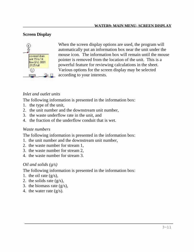
Screen Display When the screen display options are used, the program will automatically put an information box near the unit under the mouse icon. The information box will remain until the mouse pointer is removed from the location of the unit. This is a powerful feature for reviewing calculations in the sheet. Various options for the screen display may be selected according to your interests.
Inlet and outlet units The following information is presented in the information box: 1. the type of the unit, 2. the unit number and the downstream unit number, 3. the waste underflow rate in the unit, and 4. the fraction of the underflow conduit that is wet.
Waste numbers The following information is presented in the information box: 1. the unit number and the downstream unit number, 2. the waste number for stream 1, 3. the waste number for stream 2, 4. the waste number for stream 3.
Oil and solids (g/s) The following information is presented in the information box: 1. the oil rate (g/s), 2. the solids rate (g/s), 3. the biomass rate (g/s), 4. the water rate (g/s).
WATER9: MAIN MENU- SCREEN DISPLAY
3-12
Oil and solids (ppmw) The following information is presented in the information box: 1. the oil rate (ppmw), 2. the solids rate (ppmw), 3. the biomass rate (ppmw), and 4. the water rate (ppmw).
Compound (ppmw) The following information is presented in the information box: 1. the name of the compound, 2. the flow rate into the unit (ppmw), 3. the flow rate into the conduit (ppmw), and 4. the flow rate out of the conduit (ppmw).
Compound flow (g/s) The following information is presented in the information box: 1. the name of the compound, 2. the flow rate into the unit (g/s), 3. the flow rate into the conduit (g/s), and 4. the flow rate out of the conduit (g/s).
Fraction air loss The following information is presented in the information box: 1. the loss of waste over the unit (fe), 2. the loss of waste down the hub (fe), 3. the loss in the unit (fe), and 4. the loss in the line (g/s).
Ventilation The following information is presented in the information box: 1. the flow out of the unit, 2. the pressure at the unit and the downstream unit, and 3. the headspace flow in the underflow conduit.
WATER9: MAIN MENU- SCREEN DISPLAY
3-13
Vent parameters The following information is presented in the information box: 1. the connection of the entrance, 2. the connection of the exit, 3. the opening at the unit, and 4. the connection of the run.
Vent flows (g/s) The following information is presented in the information box: 1. the name of the compound, 2. the vent rate out of the unit (g/s), 3. the vent rate into the conduit (g/s), and 4. the vent rate out of the conduit (g/s).
Vent concentrations The following information is presented in the information box: 5. the name of the compound, 6. the vent rate out of the unit (ppmw), 7. the vent rate into the conduit (ppmw), and 8. the vent rate out of the conduit (ppmw).
Mass transfer coef. The following information about mass transfer coefficients are presented in the information box: 1. trench model, 2. Parkhurst and Pomeroy model, 3. the turbulent model, and 4. the McKay model.
Water flow The following information is presented in the information box: 1. the water flow rate, 2. the water velocity, 3. the waste underflow depth, and 4. the conduit slope.

WATER9: MAIN MENU- SCREEN DISPLAY
3-14
Show emissions image This option shows an emission image over the source of the emissions.
Show waste loading If the selected compound is present in the indicated waste streams, the waste stream inlet is shown as a double circle.
Show unit numbers The unit numbers are displayed downstream of the unit icon.
Small unit icons This option (toggle) changes the size of the unit icons.

WATER9: MAIN MENU- UNITS
3-15
Units
Edit unit defaults This option permits you to change the unit specific default properties. If you have three activated sludge basins you may change the biomass concentration and aeration rate once with this option. Your edited values for that unit will appear whenever you add a similar unit in this project.
Edit general defaults
General default set 1 This option permits you to edit general default values such as wastewater temperature, wind temperature, and wind humidity. The values that you specify in this set will override the general defaults, and permit you to develop a site specific set of general defaults for your project. You may change some of these site specific general default values later as you specify the individual unit specifications.
General default set 2 This option permits you to edit general default values for the molecular weight of the oil and the oil density, along with some of the NaUTilus specifications.
Global unit value sets This option will reset all of the values for any one specified unit type in the project.
Global input buttons This option creates a set of global input buttons that enable several what-if investigations. Pressing a button will set the indicated value throughout all units in the project.
Data quality check This option processes all project inputs to identify those values that you have specified that are outside of expected limits. You will be asked to confirm that your input is correct. This procedure is to assist you in correctly entering project inputs. It is not intended to restrict the ability to use correct inputs.
WATER9: MAIN MENU- UNITS
3-16
Unit property edit This option does the same thing as the [edit properties] button on the pop up unit menu box, except that you may access the edit properties feature directly from the main menu. When you use this feature, you must specify the number of the unit to be edited. If you do not know the line number, use the main menu to display the line numbers. The line numbers will be displayed on each line of the sheet by selecting [Screen display][Show unit numbers].
Delete a line This option does the same thing as the [delete line] button on the pop up unit menu box, except that you may delete the line directly from the main menu. When you use this feature, you must specify the number of the unit to be deleted. If you do not know the line number, use the main menu to display the line numbers.
Add a line This option does the same thing as manually adding a line with the mouse, except that you may use this feature directly from the main menu. When you use this feature, you must specify the number of the type of unit to be added. If you do not know the unit type number, enter a number from 1-10, and then edit the unit type number later. In order to add a line you should specify two unit numbers that are not already connected with a line. A new line will be placed between those two specified lines.
Copy set of units to a unit This option permits the copying of an entire block of line units to downstream of a selected unit. This option will result in two identical sets of interconnected units in the same project. To accomplish the copying, a form will appear on screen that must be completed.
Reset defaults This option changes all default values for each unit type to the original values that may have been changed manually in this project. You will need to edit each unit after selecting this option.

WATER9: MAIN MENU- UNITS
3-17
Show default data base You may view or print the entire data base of default values and input forms.
Edit default data base This will change the WATER9 program and default values. Do not use this feature if you do not know what you are doing. As a safety feature, save the program files (not project files!) so that you may be able to restore them. Other users of WATER9 may not have full compatibility with your files, depending on your changes. Suggested uses of this option include language translations and company specific features. Do not substitute one variable for another, or serious errors will occur in the WATER9 calculations.
Storage tank vapor pressure In a storage tank, the total contribution of the organic materials to the overall vapor pressure can depend on the composition of the materials in the tank. In particular, relatively high concentrations of oxygenates and alcohols can modify the chemical potential of an aqueous concentration. For future implementation.
Process tank For future implementation
Packed air For future implementation
tank dispersion For future implementation
Stripper For future implementation

WATER9: MAIN MENU- WASTE
3-18
Waste
Select compound in list This option will show a list of compounds that you have previously selected for your project. Mouse click the name of the compound that you wish to select. Your selected compound will be used as the basis of all calculations in your project, unless you request a procedure that automatically uses other compounds. Another method to select the compound is to mouse click on the compound name box at the top right of the screen, and then click on the name of the compound in the pop-up list. A shortcut to this method is to use the key combination [Ctrl]L.
Edit waste set This option will display a spreadsheet within WATER9 that you will use to specify your waste stream characteristics. The following items can be specified for each waste stream: 1. name: short descriptive text 2. solids(ppmw) 3. oil (ppmw) 4. dissolved solids (ppmw): not salts, potential biomass food 5. color: descriptive text not currently used 6. temp (C): temperature of waste stream before discharge 7. flow (l/s) 8. code: descriptive text. If "GAS" is entered in the code, a gas flow equaling
the flow specified above will be assumed for the waste input. 9. drop (cm): the distance from the end of the discharge pipe to the hub
opening. The flow of waste is exposed to the air during this drop. Enter zero or do not specify for sealed hubs.
10. radius(cm): one half the width of the discharging pipe stream 11. Compound concentration (ppmw): enter the concentration for each
compound More information about editing the waste set is presented in Section 8. When you have completed your waste editing activities, press the [return from
WATER9: MAIN MENU- WASTE
3-19
waste edit] button.
Load new waste set This feature will permit you to load an existing waste set from a different project into your existing project.
Add conventional sewer inlets to waste This option will process your wastewater data base and automatically add the following wastewater drop characteristics to all wastes which have a “S” in the waste description. This feature was developed to reduce editing time for automatic waste property importing from text files. (see below) Row = 6 temperature = 40 Row = 9 drop = 10 Row = 10 radius = 3
import standard waste print file This option will permit you to automatically import your entire wastewater data base from a data base or from a standard spreadsheet program (Excel, Lotus, Quattro Pro, etc.) The use of this option is described in detail in Section 9.
Edit compound properties This option will open a compound list of all compounds that you have previously indicated that you are using. Select from the list of compounds and an edit form will appear for the compound that you selected. The use of this compound edit form is described in Section 7.
Automatic compound properties This feature will automatically update missing compound properties. After using this feature, you may wish to review the new compound properties with the above procedure. In this procedure, values are estimated for all compound properties that are not present in the data base for selected or tagged compounds. Note: Only one compound at a time can be processed with this procedure, and this procedure will
WATER9: MAIN MENU- WASTE
3-20
continue until all of the tagged compounds have sufficient data to support the emission estimates. You may receive one of several messages during this procedure. Confirm the procedure option if you wish to complete this procedure. See Section 17 for details on making automatic property calculations. These completed compound properties will be used in the calculations, and the values of these compound properties will be included in the printed report. These values are now stored in the computer memory (RAM) and will be erased when the program ends, unless they are saved as part of your project, in a compound file with a special .ccc extension. Because of uncertainties in the biorate constants and the site-specific nature of measured biorate constants as well as the dependency on operating conditions, it is recommended that the biorates be measured or obtained from site-specific measurements. See 40 CFR Appendix C, to part 63.
UNIFAC biorate correlation Mouse clicking on this option is used to select the “Fragment biorate estimation” option. This will permit estimate of missing first-order biorates using a method based upon the UNIFAC fragment definitions for the compound. If you select this option, a check mark will appear to the left of [UNIFAC biorate correlation] on the minu. This option will then be used for automatic biorate estimation ONLY if there is a missing biorate. Manually enter a very small biorate (such as 0.00001) to prevent the estimation of biorate values for specific compounds. If you wish to remove the selection of this option, click on the option again and the check mark will be removed. With the check mark removed, the default OWPC estimation method will be used instead of the UNIFAC biorate correlation. Again, because of uncertainties in available methods to estimate the biorate constants and the site-specific nature of measured biorate constants, it is recommended that the biorates be measured or obtained from site-specific measurements. See 40 CFR Appendix C, to part 63.
WATER9: MAIN MENU- WASTE
3-21
Save list of compounds You may save your list of compounds in a special file format so that those same compounds may be loaded in future projects.
Load new list of compounds You may load a prior list of compounds into your waste data base so that those same compounds may be used in your current project.
Add compounds to list This feature will open a special utility that permits you to select compound from the master data set. The use of this utility is described elsewhere in Section 6. After completing this procedure, the compounds that you have selected are added to your project compound list. You may use the supporting compound property editing utilities to add a compound to the compounds in your project, or to add a new compound to the master list, or to change the properties of the compounds in the master list. Help note pads The help notes are provided to assist in the mechanics of using WATER9. Because this program is very different from WATER8 in program structure, you may wish to read this section carefully even if you are familiar with WATER8. Help notes are provided in sets of notes called a help note pad. You can move the pad on the screen and change the notes on the pad. This help note pad feature was designed to be used at the same time as you use the WATER9 program. At the main menu, press [help], then press [help notes]. A list of help note pads will appear that you may use to select the type of help that you wish. A notice of this manual is located at the end of the list, and this manual may be electronically accessed by using Adobe Acrobat Reader, commonly available for no cost as an Internet download. These help note pads can be called live since they can be edited as you use them and updated for next time by saving the help note pad as a file. The editing utilities are located at the base of the help note. If this is confusing to you, don’t use this feature to change the help notes! The help note pad files may be restored to their original form if you have saved a backup copy of the help note pad files. You may
WATER9: MAIN MENU- HELP NOTES
3-2
not read these help files with Windows Explorer, but some editing capability is provided by Windows Notepad. After you have selected a help note pad, press the [>>Next] and [<< Back] command buttons to change the pages in the help note pad. Move the help note pad out of the way by dragging and dropping the help note pad. See your Windows manual if you need help doing this. You may change the location or the shape of your help note. If you adjust the width of this window, the text width will automatically adjust to fill the help note pad. This help note pad will sometimes drop behind other program items if you make some of the selections on the main menu. Clicking the mouse icon on the help note pad will restore the help note pad to the front.

WATER9: MAIN MENU- HELP NOTES
3-3
minimum procedures Use this when you use WATER9 for the first time. Step by step instructions are provided to load a project, perform calculations, and write a report.
laying pipe Because this program is very different from WATER8 in program structure, these help notes guide you in the creation of flow diagrams on the WATER9 screens.
Exporting NaUTilus files This help note pad is provided to assist in automatically creating NaUTilus input files using WATER9 to specify unit properties.
New case This help note pad is provided to assist in using WATER9 to start your first new project. Step by step instructions are provided for the major operations that are required.
Using screen displays This help note pad provides assistance in using the screen display feature to examine the flow diagram.
Hints and suggestions This help note pad provides optional techniques to make your WATER9 project work easier.
Troubleshooting This help note pad is provided to answer some common questions. It is possible to update this help note by copying a update file over your existing help note file.
Compound properties This help note pad is provided for guidance in changing the compound properties of a compound in your project. Remember that compound properties, especially Henry’s law constant and biorate constant are important and should be experimentally based wherever possible.

WATER9: MAIN MENU- HELP NOTES
3-4
Calculations This help note pad describes manual calculation procedures. If you are investigating your system with what-if questions, you will probably need to use the manual recalculation procedures.
Examples Three help note pads describes example projects that are available for review. These include vent and landfill, collection system, and spill examples. These example projects may be located in the examples folder.
User notes This help note pad is provided as a convenient method to save your own help notes. Use it for your notes that you wish to make available for review or for others during your use of WATER9. Add your information to this help note pad and save the information so that it will be available for future reference. Note: You may save project notes in the screen titles (top left text box) or in the
comments section under [file][project information].
WATER9: NEW PROJECT FILES
4-1
4. NEW PROJECT FILES Initial setup Mouse click [File] on the top menu. Then click [new]. Away from your computer, open the physical folder that contains drawings and data forms that characterize your system. If you cannot characterize your system, read the background documentation and then repeat this step after you have collected the supporting data. WATER9 was not designed to automatically characterize your treatment and collection system.
Selecting compounds Mouse click [Waste] on the top menu. Then click [Add compounds to list]A window will open with a list of compounds on the left. Click the ones of interest and they will appear on the list on the right. You may deselect a compound by clicking it again. You may select up to 100 compounds. Click [transfer and close] when you complete your list. The wastes are located in columns and the compounds are located in rows. Selecting waste characteristics Mouse click [Waste] on the top menu. Then click [edit wastes set]A little spreadsheet will appear with up to 100 waste streams. Each stream contains all the compounds you have selected in the previous step. You may enter your waste characterization data either now or later. Click on the spreadsheet cell that you wish to edit and then type the data entry into the text entry box at the top left of your spreadsheet. When a waste drops from a pipe to a collection unit, there is a potential for air losses from an open waste stream. Specify this drop and pipe diameter in the waste spreadsheet. When a waste drops through a hub down pipe, there is a potential for air losses as the waste flows down the pipe and as the waste flows along the line. Specify these conditions with the unit properties. If a waste is entirely in gaseous form, type GAS in the code row for that waste. If "GAS" is entered in the code, a gas flow equaling the flow specified above will be assumed for the waste input.
WATER9: NEW PROJECT FILES
4-2
Click [Return from waste edit] to close the spreadsheet. Selecting type of units Mouse click [Units] on the top menu. Then click [edit general defaults]. Change the values of the defaults as appropriate for your system. A unit conversion utility is available if needed. First click [conversions], then select the type of conversion from the list that appears below the property form. Type the value on the left and the converted units will appear on the right. Double-click the relevant data cell that you are specifying on the top right side of the form to automatically enter the converted number. Mouse click [Units] on the top menu. Then click [edit unit defaults]From the list of units on the right, select the unit of concern. Continue until you have specified the major defaults. You can edit individual unit characteristics later. When a new unit is selected after this, some of these default values will be used.
Laying pipe Now you are ready to start laying pipe! Pick a sheet from the tabs of sheets at the bottom. Next, press the unit type button and select the type of unit from the list. Place the mouse pointer at the screen location for the start of the unit line. Press the left mouse button and drag along the line position to lay pipe. Remove your finger from the mouse button to drop the pipe into place. You can optionally drop the end of the line on another unit or leave it unconnected. More information about laying pipe is provided in Section 5. You should proceed from the entrances of the collection system to the treatment system exit. Each unit line has a red end and a green end. Water flows to the green, never to the red end. To add another line to the flow diagram, start at the end of an existing line and lay another line, or begin a new set of lines at a clear location on the sheet. You can always delete lines, move lines, and change unit types later. For help in the mechanics of laying pipe or selecting unit types and positioning the units on screen, a separate section is available for [laying pipe]. After the units are placed on screen, each set of unit properties may be edited.
WATER9: NEW PROJECT FILES
4-3
Editing the properties of a unit To edit the properties of a unit, position the mouse over the larger blue circle at the node of the line, or directly under the icon of the unit. The mouse pointer will appear as a double arrow when a unit is found. Click the left mouse button without moving the mouse. A unit edit box will appear after the mouse click. A gray box will appear with the number of the unit on the top of the box. Both you and the computer can identify the units by the unit number, but you may wish to enter a more descriptive name for the unit. In the gray unit box, click the button [Edit properties]. A unit box property editing box will appear. In the top cell in the editing box, type the name of the unit. The name is limited to 18 characters. Enter or change the appropriate variable for the unit at this time. You may use the unit conversion utility as described previously. Text describing the unit will appear at the bottom of the window, over the exit buttons. When you have completed the unit property data entry, press [OK] to accept the edited values and return to the main window. You may print this screen by pressing [Print]. To exit this procedure without accepting changes, press [Cancel]. Edit the properties of each unit for which you have characterization data. You can estimate the unit specifications now and update the values later with more correct values.
General Information Now you may enter general information. Click [File] on the main menu. Click [Project information] at the bottom of the list that appears. A project information form will appear that you may complete. Press [OK] when you finish filling out the form. You may have identified more units than can conveniently be placed on one screen. A title box appears at the top of each sheet and you can name the sheet for your convenience. Edit the text in the title box.
WATER9: NEW PROJECT FILES
4-4
Waste discharges The program calculates waste flow by the specified values and by the waste entry. For the units that accept waste streams, open the gray edit unit box by clicking on the blue circle under the unit icon. Click the waste number for the waste flow into the unit. The unit may accept up to three waste streams. A list of each waste will appear on screen with the numbers and waste names that you have specified. Click the appropriate waste. After the waste is selected the number of the waste will appear on screen, over the unit. Only the last waste number selected for waste stream 1 will appear in the small circle. Complete the waste stream additions for the units. Calculations Select a compound for analysis. Click [Waste] on the main menu, then click [Select compound in list], then click the compound of interest. If you have no compounds in your list, you will be directed to select compounds now. Click the refresh button to calculate the flow rates, concentrations, bioconversion, and other factors. This may take a few minutes. You may observe the progress on the little progress bar in the center of the screen. The current procedure is identified and the progress is shown by the green bar filling the gray progress bar. Mouse click [View] on the main menu. Then click [unit summaries] to observe a summary of the calculations and a material balance. You may view the results, print the results to a printer, or save the results in a file. There are many other options for reviewing the computer output. Experiment. Last step: Click [File] on the main menu. Click [Save project] and follow the directions.

WATER9: LAYING PIPE
5-1
5. LAYING PIPE This section describes the graphical method used to represent wastewater collection and treatment units on the computer screen. The units are connected by lines that are representations of pipes, underground conduits, sewer pipes, or other conduits for the flow of wastewater. Several different screens are available for representing various sections of the total system at a site.
How do I drop the pipe into place? The mouse is used as a brush to draw units on the screen. Holding the mouse button down and dragging the mouse is analogous to dragging the brush across a canvass. The procedure is to place the mouse pointer at the beginning of a unit, press the mouse button down and hold it down, move the mouse pointer to the location for the downstream line exit, and then release the mouse button, dropping the pipe into place. The start of the pipe is the unit and the end of the pipe is the downstream conduit exit. A unit has some type of collection or treatment element and an exit conduit (line) connecting to the next unit. In the case of conventional treatment elements, the connecting conduits are defined as hard piped and sealed. Add a trench or opening in conduit type of line to the exit of the unit to account for transfer losses between treatment units. Always lay the collection system and treatment system pipes so the exit (green dot at end of pipe) is either unspecified or diverted to the unit entrance (red dot on line). You will not be permitted to connect two exits together, unless one of the exits is already connected to a unit entrance. Where would the water go? Multiple lines may end at the entrance of a unit. Only two or less flow diversion lines may be connected to a unit. Flow diversion lines are a special type of unit and are used for splitting and recycle. They exit the unit before the collection line containing the main flow exiting the unit.
WATER9: LAYING PIPE
5-2
How do I transfer the flow from a stream to a unit on a different screen? Flow of wastewater can be transferred from units presented on one screen to those on another screen. When the mouse is moved across the end of a line, the divert flow button at the top of the screen is activated. Press that button. Enter the unit number of the unit that you wish to receive the flow. Then press the [OK] button.
How Do I Edit My Pipe Definitions? Place the mouse over the unit position. The unit position contains a larger blue dot, a red dot at the exit of the line, one or more green dots from inlet streams, and a crude sketch of the unit over the unit position. The mouse icon will turn into a <-> symbol at the unit. Click to open the edit unit box. In an edit unit box, you may change the type of unit, change the unit properties, add waste streams to the unit, or in the case of flow diversion units, edit the flow diversion properties. The flow diversion properties are edited from the end of the line (green dot), not the beginning of the line (red dot). Please separate the units enough to avoid confusion. Move the units out of the way if you run into trouble. Sometimes you have multiple units with similar properties, either in series or parallel. You may save time by specifying the properties for a unit, then using the copy function in the edit unit box. Open the edit unit box for the next unit. Use paste to transfer the saved properties to the next unit. A unit has some type of collection or treatment element and an exit conduit (line) connecting to the next unit. In the case of conventional treatment elements, the connecting conduits are defined as hard piped and sealed. Add a trench or opening in conduit type of line to the exit of the unit to account for transfer losses between treatment units. Multiple lines may be connected to the entrance to a unit. Only two or less flow diversion lines may be connected to a unit. Flow diversion lines are used for splitting and recycle. They are located at the exit of the unit and before the collection line containing the main flow exiting the unit. To specify the properties of a unit, first locate the unit of interest on the screen. Place the mouse over the unit position. The unit position contains a larger blue dot, a red dot at the exit of the line, one or more green dots from inlet streams, and a

WATER9: LAYING PIPE
5-3
crude sketch of the unit over the unit position. The mouse icon will turn into a <-> symbol at the unit. Click to open the edit unit box. Flow of wastewater can be transferred from units presented on one screen to those on another screen. When the mouse is moved across the end of a line, the divert flow button at the top of the screen is activated. Press that button. Enter the unit number of the unit that you wish to receive the flow. Then press the [OK] button.
How do I remove a unit from my worksheet? Place the mouse over the unit position. The unit position contains a larger blue dot, a red dot at the exit of the line, one or more green dots from inlet streams, and a crude sketch of the unit over the unit position. The mouse icon will turn into a <-> symbol at the unit. Left mouse click to open the edit unit box. In the edit box, click on the delete line button. The unit will be removed. Toggle the line button to [move lines]. Drag the end of the unit line that remains after the unit was removed to another unit and then drop the line. Press the [connect] button to link the dropped line to the downstream unit. How do I add another unit to my worksheet? First you must disconnect the upstream unit exit to make space available for adding a unit. Place the mouse over the upstream unit position. The unit position contains a larger blue dot, a red dot at the exit of the line, one or more green dots from inlet streams, and a crude sketch of the unit over the unit position. Toggle the line button to [line draw]. The mouse icon will turn into a <-> symbol at the unit if the toggle mode is [line draw]. Left mouse click to open the edit unit box. In the edit box, click on the [break] button. The unit exit will automatically separate and leave some space for a new unit. Select the type of new unit and draw the unit line from the upstream unit to the downstream unit. Press the [connect] button to verify the links of the drawn line to the downstream and upstream unit. If you are not adding a unit between two existing units, the process is much simpler. Just draw the new unit on screen, ending at the selected downstream unit. How do I recycle waste flows? If you wish to place recycle conduits on the screen, first press the [Unit type] button and select the type of recycle line from the list. Number 47 is a general recycle line, and units 48 and 49 recycle fractions of oil or solids to other units. If there is a problem with line connections, you may use the connect units options under units. This will place the exit in each line into the unit shown on the sheet.
WATER9: LAYING PIPE
5-4
How do I add a vent line to my system? If you wish to place vent conduits on the screen, first press the [Unit type] button and select the [vent line] from the list. Unlike other types of lines, start the vent line from the end of the unit line, and drop the end of the vent to the beginning of another unit line. The vent line is an advanced feature that is not generally needed. If the unit is controlled by a control device, it is possible to add both a vent line and a generic control device, but it is much simpler to specify a control efficiency at the properties edit for the originating unit.

WATER9: SELECTING COMPOUNDS
6-1
6. SELECTING COMPOUNDS FROM DATA BASE Selection form
A multiple compound selection form will be displayed for selecting compounds for your compound list. Scroll bars are available on the left of the list of compounds on the left of this selection form. If you mouse click the name of the compound it will become highlighted and will appear on the short list of compounds on the right. Clicking the highlighted compound name a second time will remove the highlight and remove the compound from the short list.
Search utilities To find compounds quickly, type the name or part of the name of the compound in the search text box (be sure to erase the words search text from within the box!). Press the next and back buttons to search the data base. Other search options are present on the multiple compound selection form, located at the lower left of the form.
Compound property review The name of the active compound is located just below the short list. Click one of the compound names in the short list to use that compound as the active compound. Pressing the review properties button with open an edit compound property form.
SMILES data base A large data base that contains the name of the chemical, the CAS number, and a SMILES string may be used to identify compounds to add to your project files. First identify the chemical of interest in the SMILES data base. Second, obtain information about the compound, including the structure from the SMILES string. Third, enter the compound information into the master data base. Last, select that new compound for inclusion into your project.
WATER9: SELECTING COMPOUNDS
6-2
Transferring the compound list to your project When you have completed the selection of compounds, press the [transfer and close] button with a click of your mouse. The compounds that you have selected will be added to your compound list (at the end). You may repeat these procedures later to add additional compounds to your project list.
Saving the compound list When you have completed your project list, you may save the list of compounds as a specially named compound file. This specially named compound file may be easily used to add a compound set to a future project without the need to manually select each compound. Select [Waste] from the main menu. Then press [save list of compounds]. You then will be prompted for a name for your compound list. Press the [save] button when you have entered the name of your compound list file.
Compound lists associated with project files Your project set of compounds will automatically be saved as you save your project file, together with compound properties that you have entered, or that WATER9 has estimated. When you load the project file that you have saved, the compound information will be the information that you had previously entered for the compound edit (see next section). These compound properties may differ from the compound properties in the main data base.

WATER9: EDITING COMPOUNDS
7-1
7. EDITING COMPOUND PROPERTIES Edit form
On the Compound Properties Editing Form, there are compound property text entry boxes that are used to specify compound properties. After complete ting the compound property editing, press [OK] to save the compound properties and close the form. Next, you may press [Master] to save the compound properties in the master data base file.
Active editing help On the Compound Properties Editing Form, there is a command button [Help off]. Press that button with the mouse and the command button will read [Help on]. Active help for this compound editing form will be enabled. At each relevant compound property text entry box, the values for the compound are estimated with a variety of methods.
Compound fragment editing On the Compound Properties Editing Form, there is a long command button on the bottom center of the form that contains the UNICAC code for the compound. Press that button with the mouse to open the Edit UNIFAC Code Form. In the edit UNIFAC code procedure, chemical compounds are described in terms of one or more chemical structures referred to as fragments. This form and its procedures allow you to identify fragments or chemical structures that are contained in the chemical compound. The compound you selected for evaluation will appear in the Edit UNIFAC Code Form. There is a set of UNIFAC supported chemical compound fragment structures listed (middle column) with their structural groups (right column). Type in revisions or additions to the compound name and the number of fragments as desired. If you do not wish to modify the UNIFAC parameters of any compound(s), press [cancel] for no selection. You can then proceed

WATER9: EDITING COMPOUNDS
7-2
to another procedure in the Compound Property Editing Form. After editing the compound’s UNIFAC parameters, press [OK].
If you have entered incorrect data or if the data do not agree with the molecular weight that is in the master compound file stored in memory, a HELP Message may appear. A typical message would be:
You may update the molecular weight in the data base if you continue.
You may select [OK] or [Cancel] The edited values of the UNIFAC code are retained in computer memory (RAM). The edited UNIFAC code will be presented in Compound Properties Editing Form, on the command button that contains the UNICAC code. In the compound properties editing form, there is a set of labels, buttons, and an input text box that can be used to add ionization constants to the data base. This set is located in the form immediately over the CAS number information. The items of this set are described below.
1. Name of the type of ionization constant for this compound. a. You will see Ka (acid) if the compound is an acid. b. You will see Ka (base) if the compound is a base. c. You will see hydrolysis rate (l/s) if the compound does not
ionize. 2. Help command button to describe the input. 3. Text box to enter the value of the constant for the compound. 4. Toggle button to change among options a,b, and c above. 5. [view] button to view the effects of pH on the compound (only for
options a and b. The equation for the ionization of an acid (AH) is as follows: Ka = [AH]/[A][H+],
where the terms in brackets [] are concentration of species and [H+] is the concentration of the ionized proton. The Ka value is sometimes listed as pKa
WATER9: EDITING COMPOUNDS
7-3
in references. pKa is the negative of the logarithm base 10 of the Ka value, similar to the definition of pH. In the case of acetic acid, the reference value of acetic acid is pKa = 4.76, Sergeant, 1979. The Ka value is then 1.74 10-5. To enter this value in the WATER9 compound data base, first select Ka (acid) and then enter 1.74E-5 in the edit box for Ka.
If you have defined a Ka value for your compound, you may press the view command button to obtain a printout of the ionization of the compound as a function of pH. Next to the value of the Henry’s law constant is the source of the data. If you have an old project file before this feature was implemented, you will not have the source of your data identified in this box. Under the name of the Henry’s law constant reference are the Henry’s law constant presented in two additional types of units. As you change the value of the Henry’s law value in the edit box, the values of the constant in these two additional types of units will automatically change.

WATER9: EDITING WASTE PROPERTIES
8-1
8. EDITING WASTE PROPERTIES Waste Edit form
This option will display a spreadsheet within WATER9 that you will use to specify your waste stream characteristics. This spreadsheet may be accessed at any time, but the editing is not permanently saved unless you save the project. If you wish to restore the waste properties, it is possible to load the previously saved project, but all editing after the last save will be lost. The waste numbers are at the top of each input column. These numbers are used to specify the waste discharge locations. If you have three waste streams with essentially the same characteristics, you only need to specify one of the streams, and that stream can be discharged in the WATER9 flow diagram in three different locations. To edit the entry in a cell of the wastewater spreadsheet, mouse click on the cell. The cell will be highlighted. Click on the edit box at the top left of the spreadsheet. Enter the desired text or numbers. Alternatively, you may press a keyboard key after you click on the cell. The keys you press after the first one will be entered into the edit box and the spreadsheet cell.
When you have completed your waste editing activities, press the [return from waste edit] button.
Waste characteristics The following items can be specified for each waste stream: 1. name: a short descriptive text that identifies the waste stream 2. solids(ppmw) 3. oil (ppmw) 4. dissolved solids (ppmw): not salts, potential biomass food 5. color: descriptive text not currently used 6. temp (C): temperature of waste stream before discharge
WATER9: EDITING WASTE PROPERTIES
8-2
7. flow (l/s) 8. code: descriptive text not generally used. If you specify GAS here, the entire
waste stream will be assumed to be in the gas phase. If "GAS" is entered as a code, a gas flow equaling the flow specified above will be assumed for the waste input.
9. drop (cm): the distance from the discharge pipe to the hub opening 10. radius(cm): one half the width of the discharging pipe stream 11. Compound concentration (ppmw): enter the concentration for each
compound this
Adding new compounds When you add new compounds to your short list of compounds, the compound names will also be added to the waste properties list.
Duplicate compounds Sometimes you may have the same compound listed more than once in the spreadsheet. Transfer the data from the second compound to the row containing the first compound, and use the delete compound button to erase the second compound from the data base. Note that you must click on the row you wish to erase before you press the delete button.
Deleting compounds Select the compound to be deleted by clicking on that row in the spreadsheet and then press the [Delete compound] button, as described above.
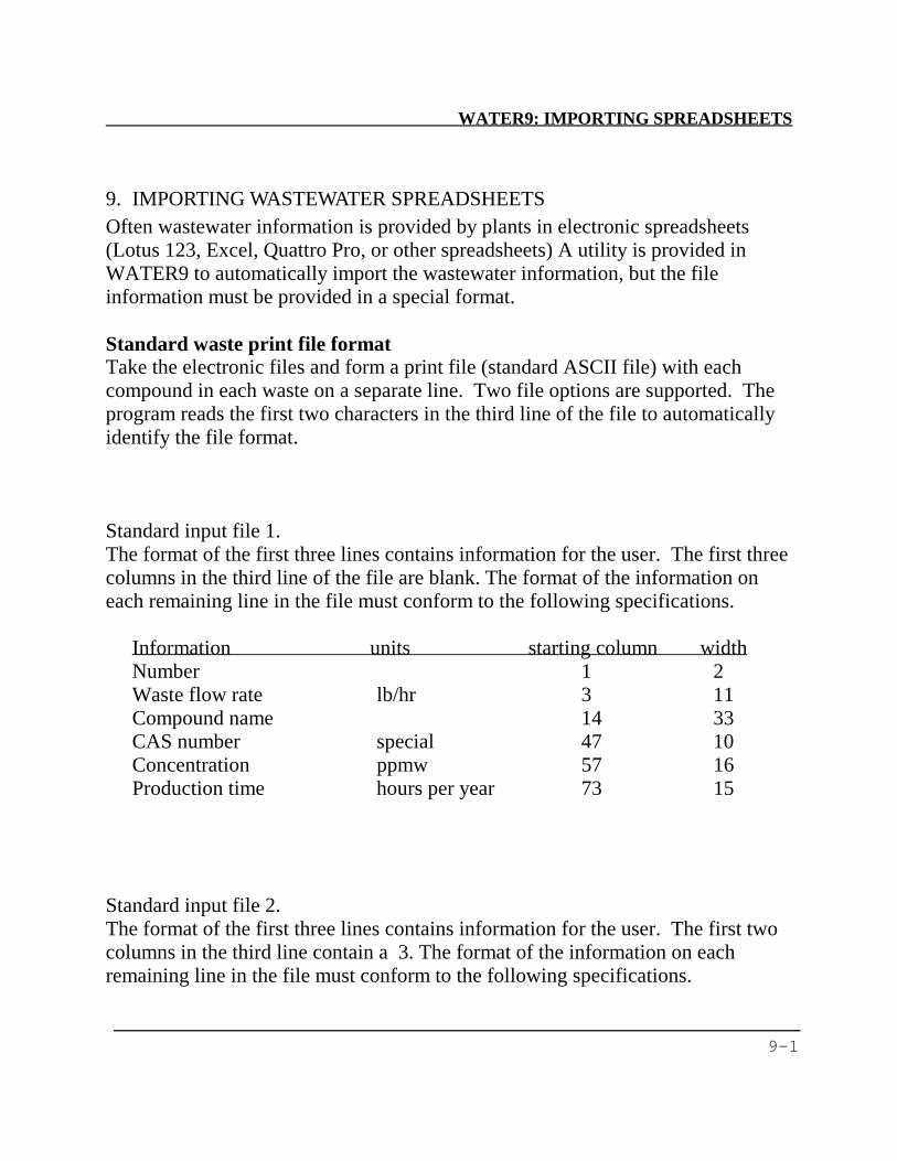
WATER9: IMPORTING SPREADSHEETS
9-1
9. IMPORTING WASTEWATER SPREADSHEETS Often wastewater information is provided by plants in electronic spreadsheets (Lotus 123, Excel, Quattro Pro, or other spreadsheets) A utility is provided in WATER9 to automatically import the wastewater information, but the file information must be provided in a special format. Standard waste print file format Take the electronic files and form a print file (standard ASCII file) with each compound in each waste on a separate line. Two file options are supported. The program reads the first two characters in the third line of the file to automatically identify the file format. Standard input file 1. The format of the first three lines contains information for the user. The first three columns in the third line of the file are blank. The format of the information on each remaining line in the file must conform to the following specifications.
Information units starting column width Number 1 2 Waste flow rate lb/hr 3 11 Compound name 14 33 CAS number special 47 10 Concentration ppmw 57 16 Production time hours per year 73 15
Standard input file 2. The format of the first three lines contains information for the user. The first two columns in the third line contain a 3. The format of the information on each remaining line in the file must conform to the following specifications.
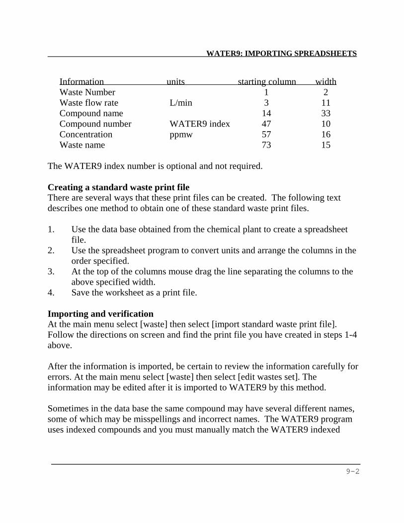
WATER9: IMPORTING SPREADSHEETS
9-2
Information units starting column width Waste Number 1 2 Waste flow rate L/min 3 11 Compound name 14 33 Compound number WATER9 index 47 10 Concentration ppmw 57 16 Waste name 73 15
The WATER9 index number is optional and not required. Creating a standard waste print file There are several ways that these print files can be created. The following text describes one method to obtain one of these standard waste print files. 1. Use the data base obtained from the chemical plant to create a spreadsheet
file. 2. Use the spreadsheet program to convert units and arrange the columns in the
order specified. 3. At the top of the columns mouse drag the line separating the columns to the
above specified width. 4. Save the worksheet as a print file. Importing and verification At the main menu select [waste] then select [import standard waste print file]. Follow the directions on screen and find the print file you have created in steps 1-4 above. After the information is imported, be certain to review the information carefully for errors. At the main menu select [waste] then select [edit wastes set]. The information may be edited after it is imported to WATER9 by this method. Sometimes in the data base the same compound may have several different names, some of which may be misspellings and incorrect names. The WATER9 program uses indexed compounds and you must manually match the WATER9 indexed

WATER9: IMPORTING SPREADSHEETS
9-3
compounds to the compounds that you have imported. Fortunately, WATER9 has utilities that greatly assist in this effort. At the main menu select [waste] then select [add compounds to list]. You may search for a compound in the data base by name (or part of a name), by molecular weight, by CAS number, or by the number of a particular chemical fragment in the compound structure. The command buttons [next] [back] and [tag] are used to scan the data base for compounds which match the criteria. You may review the properties to verify the compound match. This form can also be used to add the desired compound if it is not in the data base. The bottom line in the Multiple Compound Selection Form is used to update or replace compound names that you have already imported from the standard waste print file. The bottom line is used to match the imported compound name with the WATER9 compound name in the data base. Press [Next] and [Back] to load the imported compound names into the slot at the bottom right of the form. Pressing the [Update Compound] button will automatically replace the imported compound name in the slot with the data base name (as shown in the other slot immediately below the short list on the form). The imported compound will then be automatically indexed to the data base structure. A different method for importing spreadsheet information is described on page 3-1. The method described in this section is useful for selected types of existing spreadsheets.

WATER9: CONTROL BUTTONS
10-1
10. CONTROL BUTTONS Draw mode button Sometimes you may wish to disable the ability to draw units on the screen. Three different drawing modes are available, and the name on the draw mode button indicates the current mode. There is a button on the right of the main screen that has a title of toggle. There are three modes controlled by this toggle: lines off, draw lines, and move lines. Change the mode of drawing lines by clicking on this toggle button with your mouse [left mouse button click].
Toggle: draw mode In this mode you will be able to drag and drop new units into your flow sheet. If you accidentally start a unit addition on screen in the draw lines mode by dragging the mouse pointer across the screen with the button pressed, it is not a real problem. Drag the mouse pointer back to the start of the unwanted line and drop it there by releasing the mouse button. The unwanted line will not be placed because it would have been too short. You can delete the new unwanted line by clicking on the unit associated with the line and selecting [Delete line] from the pop-up window.
Toggle: lines off In this mode you will not change the flow sheet even if you press the mouse button. The lines off drawing mode may be helpful to avoid unintentional addition of additional units on the screen.
Toggle: move lines In this mode you will be able to move units from one place to a different place on the flow sheet. The image of a hand appears for your mouse icon. Drag and drop units with the hand. There are three hand displays: • open hand- scanning the sheet, looking for unit connections to move, • thumbs up- icon is over a connection to move, and • fist closed- mouse button is down and the unit connection may be dragged to a
different location on the sheet.

WATER9: CONTROL BUTTONS
10-2
In the move lines mode, the existing units may be moved. The line connections to the actual unit move with the unit. All other connections, including the unit conduit exit connection will not move. In the move lines mode, the mouse pointer will be a hand. Locate the magnet to a unit node, depress the mouse button (hold down) and used the closed hand to drag the unit connection to a new location. The unit will drop in place when you release your finger from the mouse button. If for some reason you want to move an unattached exit conduit, use the hand drag and drop on the unattached conduit end. To recycle or divert two lines are added. The first is the divert point. The second is a line from the end of the divert point conduit to elsewhere. Calculation button The [Update] or [Refresh: calculate] button is used to calculate the ventilation rates, the head space concentrations, and the fate of the compounds in the system. Changing the specifications at one unit may change the calculations throughout the entire system. You will not need to manually recalculate when you use the report options under [view] on the main menu. The calculations will be automatically done for those procedures. This button is used primarily for what-if user directed investigations. Divert from unit button Sometimes you will need to connect the outfall from one unit to the entrance of another unit not shown on the screen. As you pass the mouse icon over the unit of interest, you will note that the divert button at the lower left of the screen will identify the last unit that you have indicated by the position of the mouse icon. Press the divert button with a mouse click. An edit box will appear on screen. Type in the number of the unit you wish to transfer the waste to, and then press [OK]. Divert to waste button Sometimes you will need to connect the outfall from one unit to the waste discharge line at another unit. WATER9 treats waste discharge lines differently

WATER9: CONTROL BUTTONS
10-3
than line flow into a unit entrance. In order to model the air emissions from the waste discharge and drop into the unit, you should specify the originating unit discharge as a waste and specify the receiving unit waste as the waste that you have specified. Only use this waste stream at one unit. This is unlike other waste streams, since the other type of wastes may be used at more than one unit. Press the transfer button with a mouse click. An edit box will appear on screen. Type in the waste number that you wish to use to characterize the unit output, and then press [OK]. You may wish to use [Edit waste set] to obtain an unused waste number. Divert flow button If you move the mouse across the end of a divert flow line, or the start of a vent line, a divert flow button will be visible with the number of the diversion line on it. Pressing the button under that condition will open a flow diversion edit box. A flow diversion edit box will appear on screen. Type in the information about the flow diversion and then press [OK]. It is difficult to edit diversion lines when two or more diversion lines discharge into the same unit. WATER9 identifies diversion lines by the location of the end of the discharge line. When two discharge lines are located at the same place on the sheet, WATER9 can identify only one of the units. A scroll bar is present on the window below the edit flow diversion button to manually change the unit that can be edited with the use of the edit flow diversion button. This scroll bar will automatically scan the units to select flow diversion units that can be edited. Connect button Press this button if you suspect that your editing and moving the lines may have caused a problem with the flow connections between units. Things that cause problems include putting one unit on top of another and operations not previously identified in program debugging. If there is still a problem, you may wish to consider deleting the offending units and adding new units of the same type.
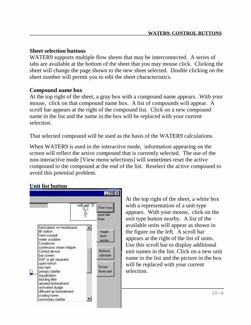
WATER9: CONTROL BUTTONS
10-4
Sheet selection buttons WATER9 supports multiple flow sheets that may be interconnected. A series of tabs are available at the bottom of the sheet that you may mouse click. Clicking the sheet will change the page shown to the new sheet selected. Double clicking on the sheet number will permit you to edit the sheet characteristics. Compound name box At the top right of the sheet, a gray box with a compound name appears. With your mouse, click on that compound name box. A list of compounds will appear. A scroll bar appears at the right of the compound list. Click on a new compound name in the list and the name in the box will be replaced with your current selection. That selected compound will be used as the basis of the WATER9 calculations.
When WATER9 is used in the interactive mode, information appearing on the screen will reflect the active compound that is currently selected. The use of the non-interactive mode [View menu selections] will sometimes reset the active compound to the compound at the end of the list. Reselect the active compound to avoid this potential problem. Unit list button
At the top right of the sheet, a white box with a representation of a unit type appears. With your mouse, click on the unit type button nearby. A list of the available units will appear as shown in the figure on the left. A scroll bar appears at the right of the list of units. Use this scroll bar to display additional unit names in the list. Click on a new unit name in the list and the picture in the box will be replaced with your current selection.
WATER9: CONTROL BUTTONS
11-5
You may now use the new unit type that you have selected as the basis for additions to the flow diagram. Straighten button The display of units on the WATER9 flow sheets are positioned in the locations that they are placed. These units may be moved by dragging and dropping in the [toggle: move mode]. This manual placement may not be visually satisfactory in some cases; therefore, an automatic procedure is available with the [Straighten] button. This button will change the location of units that are only approximately aligned horizontally and vertically so that they become exactly aligned horizontally and vertically. In some cases it may be necessary to press this button more than once. If the unit location information is needed for dispersion modeling, DO NOT PRESS THIS BUTTON.
11. IMPORTING WATER8 FILES By far the easiest way to generate a new WATER9 project file (case study) is to use WATER9 to import an existing WATER8 file to automatically create a new WATER9 project. If you are familiar with WATER8, it may be helpful to import WATER8 files and practice editing them with this program. Potential concerns There are two potential concerns to changing from WATER8 to WATER9: a more current (powerful) computer system could possibly be needed and WATER9 files may not be translated to WATER8 (no backwards compatibility). WATER9 was designed to run on a Pentium PC with at least 16M RAM. Multimedia and high resolution screens are helpful. WATER8 will run on almost any IBM compatible PC. The RAM use is very limited in WATER8.
WATER9: IMPORTING WATER8 FILES
11-2
WATER9 files may not be translated to WATER8, unless you wish to do the translation manually. Consequently, work performed on the WATER9 version of the case study will not be available for automatic translation to WATER8. Enhancements in WATER9 When a waste drops from a pipe to a collection unit, there is a potential for air losses from the open waste stream. WATER9, unlike WATER8 will include these emissions in the total emissions inventory. Unlike WATER8, since WATER9 is graphically based, it is possible to import unit locations from a spreadsheet. The output from WATER9 can be directly coupled with local dispersion models. The alignment of WATER9 will be top of sheet is North. The WATER8 collection units will be imported with a special code that permits the underflow headspace rate to be specified by the vent velocities. It is possible to manually set this code by the use of the main menu. First press [File] and then press [Specify calculation parameters]. Set the specified line vent rates to 1 for to use the vent rates for the underflow headspace rates. When WATER8 files are imported, WATER9 will automatically set this code to 2. A special code of 2 will provide an unlimited supply of clean ambient air to the underflow conduit at the end of the line downstream of the unit. WATER9 permits many different simultaneous waste discharges to the system. You will need to manually add additional wastes and waste discharge points to the imported WATER8 file. How do I import WATER8 files? Mouse click on [File] in the main menu. Mouse click on [New Project] in the secondary menu to clear previous work. Click on the [O K] button to confirm erasing previous data. Mouse click on [Import WATER8 file] in the secondary menu. Locate and open a WATER8 file using the file directory window. You should now see a flow diagram on your screen. If you had both collection units and treatment units in WATER8, these units will appear on different screens. Mouse click the [sheet 2] button to view the second sheet if WATER8 had both collection units and treatment units.
WATER9: IMPORTING WATER8 FILES
11-3
Mouse click on [Refresh calculate] button at the right of the Main window. You will notice calculation information appearing during calculation. Mouse click on [View] on the main menu. Mouse click on [Detailed calculation details] near the bottom of the drop down menu list. A display will appear. You may view the calculations by clicking the [page up] [page down] buttons. Click [Print] to direct the results to a printer. [File] prints to disk. You may also save as a comma separated value file for importing into a standard spreadsheet program. A comma separated value file is inappropriate for this type of display. To complete the importing of a WATER8 file, you should save your work. Mouse click [File] on the main menu. Then click [Save project]. Name the file using a [.WWD] extension and then save the file. You have now completed the WATER8 import process. Editing your work and verification Unlike in WATER8, WATER9 is able to transfer the flow of wastewater from the collection system units presented on one screen to those on another screen. Identify the unit number of the destination unit. Next locate the origination unit. When the mouse is moved across the end of a line, the divert flow button at the right of the screen is activated. Press that button. Enter the unit number of the unit that you wish to receive the flow. Then press the [OK] button. It may be useful to rearrange units using the toggle move lines button, especially if clarifier recycle is added to the system. The automatic layout provided by importing WATER8 files may be less useful in some cases than a custom layout. You can load a WATER8 file, and the program will automatically transfer the compounds in the *. ccc compound file into WATER9. Because WATER9 is very different from WATER8 in program structure, you can not save WATER9 information in a WATER8 format. You may delete the units definitions in WATER9 and retain the compound list for another project.
WATER9: NaUTilus COMPATABILITY
12-1
12. NaUTilus COMPATABILITY NaUTilus is a compiled computer program that was developed at the University of Texas at Austin. It is a Fortran based text interpreter program that estimates air emissions from collection systems based upon input files provided by the user. There are two different programs in NaUTilus, one for inside the battery limit, ISBL (a battery limit is the physical boundary around a process unit) and one for outside the battery limit, OSBL. WATER9 has the capability to write input files for NaUTilus for both types of NaUTilus programs. You can save your WATER9 project file work as NaUTilus input files that can be processed with the program NaUTilus. Because WATER9 is very different in program structure from NaUTilus, you may not save all WATER9 file structures as a NaUTilus file. Read the following sections for the procedures needed for generating NaUTilus files. The contents of screen 1 will be saved as an ISBL network map. The inside battery limit inputs support drains, hard pipe lines, manholes, and drops. Unit types not supported by NaUTilus on screen 1 will be translated to NaUTilus as sealed nodes. The contents of screen 2 will be saved as a OSBL network map. The outside the battery limit inputs support reaches, manholes, and drops. Unit types not supported by NaUTilus on screen 2 will be translated to NaUTilus as sealed nodes. Remember to edit the units to verify that sealed drains have an opening size of zero. After you have filled out the forms for Screen 1 and Screen 2, you may proceed with generating NaUTilus input files. First, save your work. Next, mouse click the file option at the upper left of the WATER9 window. Then select Save as NaUTilus input file. At this point it is important to wait for at least 30 seconds to permit the NaUTilus program to process the data and present you with files to review on your WATER9 screen.
WATER9: NaUTilus COMPATABILITY
12-2
The NaUTilus input files will be saved automatically in the working directory. This completes the procedure. When you run NaUTilus, these files that you have created will be automatically processed by NaUTilus and the proper output files will be written. When you write the files for NaUTilus, the program will automatically run the NaUTilus programs. After a 15 second delay, the program will then read the NaUTilus input and output files. For an example, load the file ISBL and examine the arrangement of the units and the waste. When you save as a NaUTilus file, you must wait for the NaUTilus display or you may cause program errors. This is due to automatic file number use in the shelled executable files. WATER9 must reset the files after internally running NaUTilus.
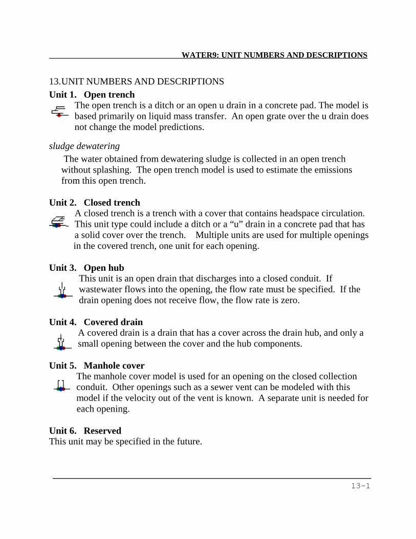
WATER9: UNIT NUMBERS AND DESCRIPTIONS
13-1
13. UNIT NUMBERS AND DESCRIPTIONS Unit 1. Open trench
The open trench is a ditch or an open u drain in a concrete pad. The model is based primarily on liquid mass transfer. An open grate over the u drain does not change the model predictions.
sludge dewatering The water obtained from dewatering sludge is collected in an open trench without splashing. The open trench model is used to estimate the emissions from this open trench.
Unit 2. Closed trench
A closed trench is a trench with a cover that contains headspace circulation. This unit type could include a ditch or a “u” drain in a concrete pad that has a solid cover over the trench. Multiple units are used for multiple openings in the covered trench, one unit for each opening.
Unit 3. Open hub
This unit is an open drain that discharges into a closed conduit. If wastewater flows into the opening, the flow rate must be specified. If the drain opening does not receive flow, the flow rate is zero.
Unit 4. Covered drain
A covered drain is a drain that has a cover across the drain hub, and only a small opening between the cover and the hub components.
Unit 5. Manhole cover The manhole cover model is used for an opening on the closed collection conduit. Other openings such as a sewer vent can be modeled with this model if the velocity out of the vent is known. A separate unit is needed for each opening.
Unit 6. Reserved This unit may be specified in the future.

WATER9: UNIT NUMBERS AND DESCRIPTIONS
13-2
Unit 7. Open sump This unit type is used for units that have wastewater flow across an open tank, box, or conduit section. The depth of flow across the box is a required input. The depth of flow is estimated as the depth of the inlet
conduit bottom. The flow of inlet wastewater across the surface of the sump is used to estimate the mass transfer within the sump. Waterfalls within the sump are not addressed with this model. The flow of entering water is either subsurface or the top surface of the entrance is approximately even with the level of the top surface of the sump.
Unit 8. Closed sump, vent
This unit type is used for units that have a sealed cover and wastewater flow across a covered tank, box, or conduit section. The depth of flow across the box is a required input for mass transfer estimates in the unit.
The depth of flow is estimated as the depth of the inlet conduit bottom. The vent height and diameter should be specified.
Unit 9. Reserved This unit may be specified in the future. Unit 10. Opening in conduit
A sewer reach is an open or closed conduit that transfers wastewater by gravity flow. The velocity of liquid flow is specified. The velocity of flow
can be estimated by correlations or measured.
Unit 11. Open j drain The open j drain is a water trapped drain (sometimes trapped with anti-freeze for inactive drains in cold climates), with potential air emissions over the surface of the hub and in the waste drop to the hub. No headspace will flow
into or out of the hub with a j drain. Air emissions are estimated from the waste flow before the level in the trap and from waste in the trap.
Unit 12. Headspace sealed
A unit that has a sealed headspace has no air exchange between the headspace and the outside air. Mass transfer can occur between the liquid and the gas phase. Headspace exchange can occur with other units.
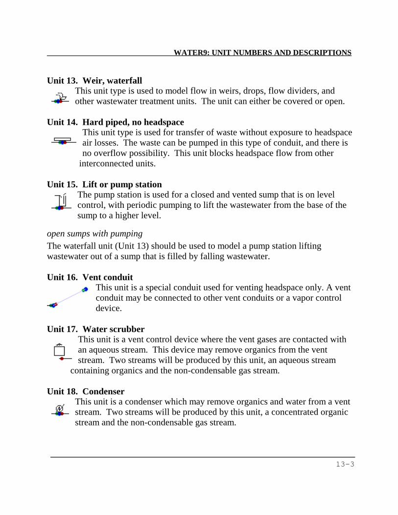
WATER9: UNIT NUMBERS AND DESCRIPTIONS
13-3
Unit 13. Weir, waterfall
This unit type is used to model flow in weirs, drops, flow dividers, and other wastewater treatment units. The unit can either be covered or open.
Unit 14. Hard piped, no headspace This unit type is used for transfer of waste without exposure to headspace air losses. The waste can be pumped in this type of conduit, and there is no overflow possibility. This unit blocks headspace flow from other
interconnected units.
Unit 15. Lift or pump station The pump station is used for a closed and vented sump that is on level control, with periodic pumping to lift the wastewater from the base of the sump to a higher level.
open sumps with pumping The waterfall unit (Unit 13) should be used to model a pump station lifting wastewater out of a sump that is filled by falling wastewater. Unit 16. Vent conduit
This unit is a special conduit used for venting headspace only. A vent conduit may be connected to other vent conduits or a vapor control device.
Unit 17. Water scrubber This unit is a vent control device where the vent gases are contacted with an aqueous stream. This device may remove organics from the vent stream. Two streams will be produced by this unit, an aqueous stream
containing organics and the non-condensable gas stream.
Unit 18. Condenser This unit is a condenser which may remove organics and water from a vent stream. Two streams will be produced by this unit, a concentrated organic stream and the non-condensable gas stream.
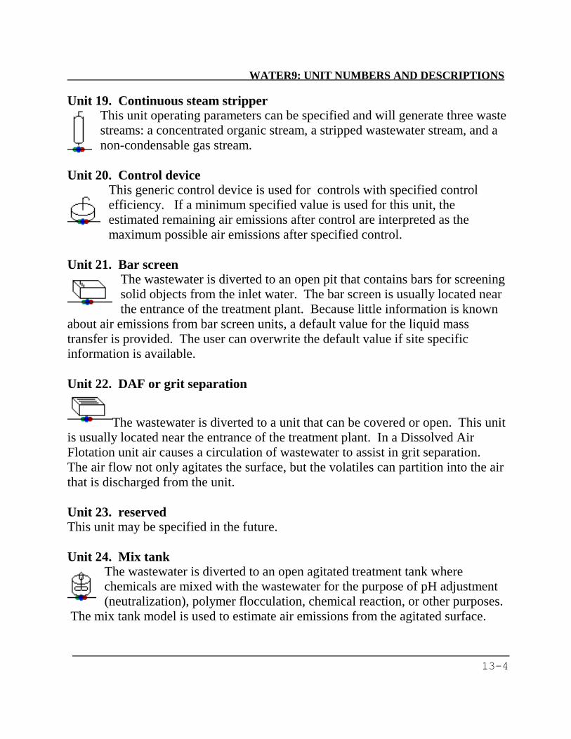
WATER9: UNIT NUMBERS AND DESCRIPTIONS
13-4
Unit 19. Continuous steam stripper This unit operating parameters can be specified and will generate three waste streams: a concentrated organic stream, a stripped wastewater stream, and a non-condensable gas stream.
Unit 20. Control device This generic control device is used for controls with specified control efficiency. If a minimum specified value is used for this unit, the estimated remaining air emissions after control are interpreted as the maximum possible air emissions after specified control.
Unit 21. Bar screen
The wastewater is diverted to an open pit that contains bars for screening solid objects from the inlet water. The bar screen is usually located near the entrance of the treatment plant. Because little information is known
about air emissions from bar screen units, a default value for the liquid mass transfer is provided. The user can overwrite the default value if site specific information is available.
Unit 22. DAF or grit separation
The wastewater is diverted to a unit that can be covered or open. This unit is usually located near the entrance of the treatment plant. In a Dissolved Air Flotation unit air causes a circulation of wastewater to assist in grit separation. The air flow not only agitates the surface, but the volatiles can partition into the air that is discharged from the unit. Unit 23. reserved This unit may be specified in the future. Unit 24. Mix tank
The wastewater is diverted to an open agitated treatment tank where chemicals are mixed with the wastewater for the purpose of pH adjustment (neutralization), polymer flocculation, chemical reaction, or other purposes.
The mix tank model is used to estimate air emissions from the agitated surface.
WATER9: UNIT NUMBERS AND DESCRIPTIONS
13-5
Unit 25. Primary municipal clarifier
The wastewater is diverted to a large open circular holding tank where solids can settle. The water exits the clarifier by flowing over a weir around the edge of the clarifier. The dimensions of the overflow are needed for the clarifier model. The primary clarifier is located
before the biological treatment, and the secondary clarifier is located after the biological treatment. Use the secondary clarifier model instead of the primary clarifier for industrial wastes.
rectangular clarifier and double weirs If the clarifier is rectangular, the equivalent diameter is 1.13 times the square root of the area (m2). The equivalent fraction of the perimeter for the weir is the actual perimeter divided by the product of 3.141592 and the equivalent diameter. A second weir can be added to the model by
placing a waterfall unit (Unit 17) after the clarifier. Unit 26. Equalization
The wastewater is diverted to a large tank or holding pond that is used to provide a more uniform concentration of chemicals in the wastewater before biodegradation. The equalization unit is located before biological treatment. Agitators are sometimes used to promote mixing and cool the wastewater.
High temperatures in biotreatment can cause reduction in the flocculation settling rates. The model for equalization is flexible and can model several types of equalization units.
equalization pond, plug flow
The wastewater is diverted to a large holding pond that is used to provide a more uniform concentration of chemicals in the wastewater before biodegradation. The equalization unit is located before biological treatment. Agitators are sometimes to used to promote mixing and cool the

WATER9: UNIT NUMBERS AND DESCRIPTIONS
13-6
wastewater. The equalization model should be used with the flag set for plug flow for ponds that are very large, segmented, or have specific agitated zones.
Unit 27. Trickling filter
A trickling filter is a bed of support materials that the wastewater is recirculated over. Tricking filters can be natural draft or forced draft. The support solids contain a layer of biologically active material. Worksheets are used to estimate parameters for the loss
in the spray to the surface and in the mass transfer from the liquid to the air.
cooling tower with biological activity A cooling tower that supports biomass could operate in a similar manner to a trickling filter. The use of the trickling filter unit can be used to estimate the cooling tower emissions with biodegradation but it cannot be used to estimate temperature effects. An average temperature must be provided as an input value.
Unit 28. Aerated biotreatment The wastewater is diverted to a large basin that contains surface aerators. Some biomass is present in the basin. The fraction of the surface that is agitated can be evaluated with the following table.
WATER9: UNIT NUMBERS AND DESCRIPTIONS
13-7
Table 1. Turbulent Areas and Volumes for Surface Agitatorsa
ωωωω, Motor horsepower
At, Turbulent area
Effective depth
V, Agitated volume
aV, Area per volume
hp Ft2 M2 ft ft3 ft2/ft3
5 177 16.4 10 1767 0.17.5 201 18.7 10 2010 0.110 227 21 10.5 2383 0.095215 284 26.4 11 3119 0.090920 346 32.1 11.5 3983 0.08725 415 38.6 12 4986 0.083330 491 45.7 12 5890 0.083340 661 61.4 13 8587 0.076950 855 79.5 14 11970 0.071460 1075 100 15 16130 0.066675 1452 135 16 23240 0.0625
100 2206 205 18 39710 0.0555aData for a high speed (1,200) rpm) aerator with 60 cm propeller diameter (d).
Unit 29. Activated sludge biotreatment The wastewater is diverted to a large tank that is agitated and contains biomass in excess of 1 g/l. The surface is agitated with the equivalent of surface aerators. The zones of agitation will be apparent by inspection. This unit can used for submerged aeration without surface aerators, but you will need to characterize the extent of your surface
agitation with equivalent surface aerators. The fraction of the surface that is agitated is estimated by inspection if surface aerators are not present.
WATER9: UNIT NUMBERS AND DESCRIPTIONS
13-8
Unit 30. Diffused air biotreatment
The wastewater is diverted to a large tank that is agitated by diffused air bubbles. The tank generally contains biomass in excess of 1 g/l. The surface may be agitated by submerged aeration. The zones of agitation will be apparent by inspection. The fraction of the surface that is agitated is estimated by inspection. Use this unit if you do not
wish to characterize the agitation on the surface. Use the activated sludge biotreatment unit [unit 29] if you can specify the agitation parameters needed to estimate the surface mass transfer.
UNOX and closed vented system biotreatment The wastewater is diverted to a large closed vented tank that is agitated by submerged air flow. The tank generally contains biomass in excess of 1 g/l. The surface may be agitated by submerged aeration, but since the tank is closed, this does not influence the model predictions. The vented gas may contain some volatile organics, and the vent rate should be used in the model specifications. The vent rate may be somewhat lower than the inlet air rate, depending on the operation of the system. Remember to specify that the system is closed, enter [1]. Unit 31. Cooling tower
A cooling tower is often used to cool the wastewater before the wastewater contacts the biological organisms. The cooling tower can have recycled water within the unit that is specified as a unit parameter. External recycle is specified by recycle lines and flow rates. Often, only part of the overall
wastewater flow is diverted to the cooling tower. Specify the flows to the cooling tower, the flows and destination unit from the cooling tower. There are two types of cooling towers supported by WATER9, the countercurrent and the cross-flow tower. In the countercurrent tower, the air flows up as the water flows down, and in the cross-flow tower, the water flows down as water flows across the packing. Unit 32. Circular clarifier
The wastewater is diverted to a large open circular holding tank where solids can settle. The water exits the clarifier by flowing over a weir around the edge of the clarifier. The dimensions of the overflow are
WATER9: UNIT NUMBERS AND DESCRIPTIONS
13-9
needed for the clarifier model. The circular clarifier is often located before the biological treatment, and another clarifier is located after the biological treatment to remove biomass from the treated water. rectangular clarifier and double weirs If the clarifier is rectangular, the equivalent diameter is 1.13 times the square root of the area (m2). The equivalent fraction of the perimeter for the weir is the actual perimeter divided by the product of 3.141592 and the equivalent diameter. A second weir can be added to the model by placing a waterfall unit (Unit 17) after the clarifier. Consider the use of Unit 40. Unit 33. API separator or oil water separator
An API separator is a three zone unit: (1) inlet surface, (2) larger surface with floating oil covering part of the larger surface, and (3) an overflow weir. Some of the zones can be deleted from the unit by
setting the surface area equal to zero, the weir drop to zero, or other methods. If the separator is closed and vented, use the covered separator model (19). Unit 34. Storage tank
The wastewater is diverted to a set of holding tanks. The storage tank is filled and discharged periodically or continuously. There are several types of storage processes supported by the storage tank unit. The fill depth of liquid in the tank is specified as the tank height, and
the expected headspace depth is specified as the average distance between the liquid surface and the fixed roof. If a storage time of zero is specified, the holding time is estimated from the waste flow rate, the tank diameter, and the tank height. The amount of oil in the tank is specified independently from the oil in the inlet waste, because all of the inlet may not be removed from the working of the tank. Some of the major types of storage tanks are listed below. Only types A, B, and C are supported by the storage tank model (Unit 34), and other Units should be used for types D and E.
34 A. fixed roof tank model. The fixed roof tank has an open surface with partial equilibrium with the headspace. The tank is periodically filled and discharged. The extent of
WATER9: UNIT NUMBERS AND DESCRIPTIONS
13-10
equilibrium is estimated by the holding time before discharge. The material in headspace is not discharged to the atmosphere by wind flow, but only by working (filling expels headspace) and breathing (headspace expands by heating during the day). Reference AP42 storage tanks.
34 B. open roof tank model. The open roof tank has wind driven motion of headspace within the tank. This type of tank model is used whenever an area of surface exposed to the wind is specified.
34 C. constant level fixed roof tank model. The fixed roof tank has an open constant depth surface at equilibrium with the headspace. The tank is continuously or periodically filled and discharged with equal rates. This type of tank model is supported by WATER9 Unit 34 whenever the tank height is set to zero. In WATER9, several options are available to simulate a constant level tank, including manually subtracting the calculated working loss.
34 D. open roof agitated tank. This tank is open to the atmosphere, and has one or more zones within the tank that are agitated by mechanical agitation, feed flow design, submerged aeration, or other mixing methods. Use Unit 24 for tanks with agitated surfaces.
34 E. submerged aeration tank. This tank is not completely sealed to the atmosphere, and submerged aeration is used for mixing, treatment, or other reasons. Use Unit 24 for tanks with submerged aeration.
Caution: Do not use this unit for pressurized feed that flashes upon introduction
to the storage tank. Do not use this unit for permeation across a semi-permeable membrane cover. Do not use this unit for floating roofs with a continuous seal with the tank wall.

WATER9: UNIT NUMBERS AND DESCRIPTIONS
13-11
Unit 35. Oil film unit
The wastewater is diverted to a large holding pond that permits oil to float to the surface. This unit is used for estimating the air emissions from a thin film of oil. If the unit has a thick film of oil on the
surface, the model may overestimate the air emissions.
oil press separator The wastewater sludge that contains oil is treated in an oil or water separator or filter that removes the oil and water from the sludge. The oil and water is held temporarily in a pit. The pit is modeled as an oil film unit. Unit 36. Lagoon
The wastewater is diverted to a large holding pond. The contents of the lagoon are gently agitated by wind shear at the surface.
Unit 37. Biofilter This unit may be specified in the future. Unit 38. Reserved
This unit may be specified in the future. Unit 39. Covered separator
This unit is covered and removes oil from the wastewater. Some of the volatiles will be removed by the oil. A headspace purge rate is specified, and the loss to the headspace is estimated from equilibrium calculations.
Unit 40. Rectangular covered clarifier. This unit is similar to the circular clarifier, except that the unit is rectangular and covered with ventilation.

WATER9: UNIT NUMBERS AND DESCRIPTIONS
13-12
Unit 41. reserved This unit may be specified in the future.
Unit 42. reserved This unit may be specified in the future.
Unit 43. Landfill
This unit is similar to the landfill model in Chemdat8. The waste composition of the liquids in the landfill are specified in the conduit that is discharging to the landfill unit.
Unit 44. Porous solids unit The porous solids unit is used for estimating the fate of compounds in liquids contained by porous solids. The liquid is held within the porous solid matrix by capillary forces, and evaporative losses occur through
diffusion in the open air voids. Unit 45. Land treatment
This unit is similar to the land treatment model in Chemdat8. The waste composition of the liquids applied to the site are specified in the conduit that is discharging to the land treatment unit.
Unit 46. System exit stream
This unit is used to identify project exit streams. The concentrations and flow rate are estimated for the exit stream, and the estimated quantity may be compared to the measured values at the exit point.
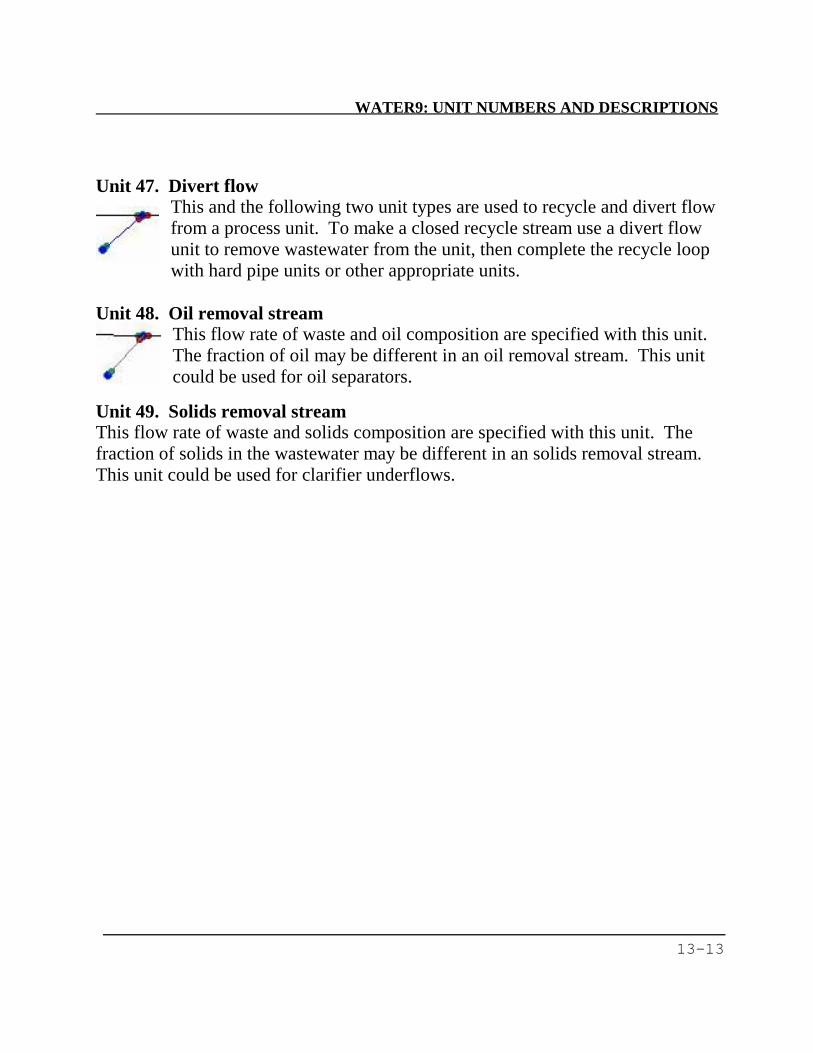
WATER9: UNIT NUMBERS AND DESCRIPTIONS
13-13
Unit 47. Divert flow
This and the following two unit types are used to recycle and divert flow from a process unit. To make a closed recycle stream use a divert flow unit to remove wastewater from the unit, then complete the recycle loop with hard pipe units or other appropriate units.
Unit 48. Oil removal stream
This flow rate of waste and oil composition are specified with this unit. The fraction of oil may be different in an oil removal stream. This unit could be used for oil separators.
Unit 49. Solids removal stream This flow rate of waste and solids composition are specified with this unit. The fraction of solids in the wastewater may be different in an solids removal stream. This unit could be used for clarifier underflows.

WATER9: DEFINITIONS
14-1
14. DEFINITIONS Discussion of Collection System Elements WATER9 represents actual collection systems by a series of elements. The elements are connected together, and each element has an underflow conduit that connects to the next downstream element. A collection system element contains two parts, a unit (drain, J trap, hub, manhole, sump, vent, or other unit) and an underflow conduit. Each element has a specification form that includes specifications for both the unit and the associated exit underflow conduit. The upstream elements including the upstream conduits that discharge into the element of concern are specified on a different form.
Definition of Terms
area of surface (cm2) (sump) The area of the surface exposed to the wind or to the headspace in a sump. This area generally corresponds to the physical area of the sump exposed surface horizontal cross-section.
area of openings at unit(cm2) The area that can vent headspace gas or permit outside air to enter the collection system. This area is generally less than or equal to the area of the drop pipe opening.
assume equilibrium in unit, =1 If condition are present in the unit such that equilibrium is expected (agitated surface, sealed waterfall, splash loading, low gas and liquid flow, or other factors) enter a 1 as a computer flag.
cover An enclosure that prevents the exchange of ambient air and the headspace air. If there are openings in the cover, then air may be exchanged with the headspace air. The openings in the cover are specified as area of openings at unit.
covered, then enter 1 The input value is a computer program flag that specifies that the unit is sealed and outside wind will not blow across the surface of the liquid in the unit. If the unit is covered, this does not indicate that the surface of the liquid is not exposed to headspace gas.
depth of liquid in sump (cm) The depth in centimeters from the top of the liquid surface in the sump to the base of the sump. The depth is always positive.
depth of water level (cm) (J trap) The depth in centimeters from the top of the liquid surface in the water seal to the base of the water seal. This depth is

WATER9: DEFINITIONS
14-2
always positive and would correspond to the wet distance on a dip-stick. This variable may be used for periodically active hubs.
description of unit This is a general description that identifies the unit that is being specified. Examples can include “Tank A45", “Drain E-17", “Sewer WW4", or other description. This description will appear on some of the reports.
displacement in oscillation (cm) (J trap) Distance of surface level fluctuation in the J trap. The value of the displacement is used in an air emission model to estimate air exchange.
distance to trap liquid surface (cm)(J trap) The depth in centimeters from the top of the open hub top to the liquid surface within the J trap. The depth is always positive and would correspond to the dry distance on a dip-stick.
distance to next unit (cm) The distance of the run of the underflow conduit that connects the unit to the next unit downstream.
drop length to conduit (cm) The length in centimeters from the top of the hub in the drop pipe to the typical liquid surface in the underflow conduit. The length is always positive.
drop length to conduit (cm) (J trap)The length in centimeters from the water seal in the J trap to the typical liquid surface in the underflow conduit. The length is always positive.
flow entrance depth under surface (cm) The area of fractional approach to equilibrium The fraction of equilibrium between the liquid
and the headspace in the lift station unit. To use a mass transfer model, consider using the waterfall unit.
headspace The headspace is the air over the wastewater in the enclosed underflow conduit.
municipal waste in conduit =1 The input value is a computer program flag which identifies which mass transfer model is used for the calculations. Zero is the default value, 1 is the Parkhurst-Pomeroy correlation for municipal sewers, and 2 is the trench model based on correlations by Owens.
open surface=1 (J trap)The input value is a computer program flag which indicates that the surface of the unit receiving the waste is open to the atmosphere. Zero is the default value, and it is considered very unusual to use an open J trap for discharge into an unit with an exposed surface.
open surface=1 (sump) The input value is a computer program flag which indicates that the surface of the unit receiving the waste is open to the

WATER9: DEFINITIONS
14-3
atmosphere. Zero is the default value, and a value of 1 indicates that there are potential air emissions from wind blowing across the surface. Grates and perforated covers are considered characteristic of an open surface.
open surface=1 The input value is a computer program flag which indicates that the surface of the unit receiving the waste is open to the atmosphere. Zero is the default value (closed unit). This flag does not refer to the underflow conduit, only to the units. The flow of headspace in the drop pipe will be of less importance if the drop pipe connects to an unit that is open.
oscillation cycle time (min) The cycle time or period of the water level rise and drop in an open water trap. Variations in the internal headspace pressure will cause water level oscillations.
radius of underflow conduit (cm) One half the diameter of a circular exiting pipe that connects the unit to the next unit downstream. This pipe is considered closed and not exposed to leaks and air exchange with the environment during the run of the pipe. If the conduit is not closed, consider the trench model.
radius of drop pipe (cm) (J trap) The radius in centimeters in the drop pipe forming a water seal in the J trap. The drop pipe connects the hub to the water seal in the J trap.
radius of drop pipe (cm) The radius in centimeters in the drop pipe that connects the hub to the unit. There is no water seal on the drop pipe (see J trap).
rise The difference in elevation in an underflow conduit that connects collection system units.
run The path in an underflow conduit that connects collection system units. slope of underflow conduit The ratio of the rise to the run in the underflow
conduit. The slope is always positive and measured from downstream to upstream in each run.
subsurface exit =1 This input value is a computer program flag which indicates that the headspace is blocked from flowing into or out of the underflow conduit downstream. A value of zero indicates that there is no headspace blockage.
subsurface entrance=1 This input value is a computer program flag which indicates that the headspace is blocked from flowing into or out of the upstream underflow conduits. A value of zero indicates that there is no headspace blockage.
total water added at the unit (l/s) This is the amount of water added at the unit, in
WATER9: DEFINITIONS
14-4
excess of specified wastewater flow into the collection system and in excess of wastewater flow from upstream underflow conduits.
underflow Temperature (C) The entrance temperature of the liquid into the unit. The temperature of the waste stream is specified separately.
underflow conduit The exiting pipe or trench that connects the unit to the next unit downstream. This conduit may be (1) closed and not exposed to leaks and air exchange with the environment during the run of the pipe or (2) exposed to leaks and air exchange with the environment.
velocity air at opening (ft/min) The velocity of flow into the unit at the specified unit openings (see area of openings at unit). This value is only used if a special flag is set. (See Form 6 general specifications 22. specified line vent rates, =1)
waste added to system at unit number The input information of waste streams into the collection system units is accomplished by specifying the waste number. The waste number refers to a data base element that includes the drop distance into the hub, the flow rate, the temperature, concentrations, the oil content and other information.
waterfall drop height (cm) The distance from the top of the waterfall to the tail water surface level (unit liquid underflow level) . This value is always positive.
waterfall: tail water depth (m) The depth of flow in the underflow conduit under the waterfall.
waterfall: Open surface=1 The input value is a computer program flag which indicates that the waterfall is open to the atmosphere. Zero is the default value (waterfall is enclosed).
waterfall width at surface (m) The width of the waterfall across the at the upper liquid level. The flow rate is used with the width to estimate the thickness of the falling water film.
WATER9: TROUBLESHOOTING
15-1
15. TROUBLESHOOTING PROCEDURES Problems and Solutions
How do I inspect the characteristics of a unit that I am concerned about?
Answer: Mouse left click on the blue dot under the unit icon on the screen. A pop-up window with a view button at the lower right will appear. Mouse click the view button. A report of the unit characteristics will appear that can be reviewed or printed as a report.
The information about the unit doesn't seem to reflect the input properties.
Answer: Repeat the calculation procedure several times after you first recalculate
the project results. The calculations may take a few seconds and in some cases can be highly interactive with other calculations. The project must be manually recalculated to inspect the effects of changes in specifications, even after loading without changes in input parameters. These recalculation problems are due to the recycle of wastewater or headspace upstream in the plant. Repeated calculation of the entire plant will improve the accuracy of WATER9.
How do I check to see if the calculations are reasonable and consistent?
Answer: Run a material balance under [view] on the main menu. Use the [display
view] options under the main menu. Select the unit with a pop-up menu and press [view] on the pop-up menu for a unit specific material balance and calculation details. A detailed report for that unit will appear that can be reviewed or printed as a report.
Somehow, a unit does not exit in the specified system as the unit shown on the screen. Answer: Use reconnect units option under the Unit menu option. This will
automatically reestablish the unit connections as shown.
WATER9: TROUBLESHOOTING
15-2
There is a problem with the apparent accuracy of the WATER9 calculation for my system. What should I do? Answer: The following steps may be of help:
• Use reconnect units option under the Unit menu option. This will automatically reestablish the unit connections as shown.
• Use the update button to repeat the calculations several times for a compound. If the results of the calculations keep changing, there is a convergence problem.
• Check the unit specifications for errors. • Try simplifying your system if it is very complex. • Report the problem as a potential program error.
I have read the instructions, and am very confused about how to start using WATER9. It seems much too complicated. What should I do? Answer: Start simply by using [File] [load] to load one of the example projects
that were provided with WATER9. Explore the loaded project by selecting various [view options]. Then try [screen display] options with the use of the mouse pointing to different units on the screen. Next, select another compound by clicking on the compound name in the gray box and then clicking the name in the compound list that appears. Next edit the properties of a unit and observe changes in the WATER9 calculations. These exercises should make you much more comfortable with the WATER9 features. Next, try some of the help features.
How do I add a unit? You cannot add a unit between two other units.
Answer: That is correct, so you need to break the connection between two units. Break the connection by opening the upstream unit edit box and then using the [break] button. This will break the connection between the two units, leaving a place for adding a unit between the units. Use the move feature to rearrange the locations of the units on the screen.

WATER9: TROUBLESHOOTING
15-3
My units are too close together to work easily. How can I fix this problem?
Answer: There are several options. Move some of the units to another sheet,
rather than loading many units on one sheet. Make the screen larger and separate the units (this assumes that your screen resolution is higher than minimum). As a last resort, try then using the smaller unit icon option under [Screen display].
My eyesight is not good enough to read the on-screen display. How can I fix this problem?
Answer: There are several things that may help. Your windows setup should have
a large font option. Make the screen smaller (this assumes that your screen resolution can be reduced). Try the larger font unit display text option under [Screen display]. This will increase the size of the font in the screen display boxes.

WATER9: UNIFAC CALCULATIONS
16-1
16. UNIFAC CALCULATIONS The UNIFAC (UNIquac Functional-group Activity Coefficient) model is a method of predicting solute-solvent interactions so that Henry’s law constants, partition factors, and solubility limits can be estimated for complex mixtures. Computer subroutines were written and included in the computer program to make the calculation procedure less tedious.
Background to UNIFAC The UNIFAC method of Fredenslund et al. (1975) is described by Arbuckle (1983) as useful for predicting Henry’s law constants (+/-0.112 log units), octanol-water partition coefficients (+/-0.333 log units), and solubilities (+/-0.418 log units). See also Georgeton and Sommerfield (1983) for a discussion of vapor-liquid equilibria estimation with UNIFAC. Although UNIFAC is not necessarily accurate in all cases and interaction data are absent for some compounds (restricting use of the model), the method is considered to be the most generally reliable technique for estimating a component’s activity in the absence of reliable measured data. The UNIFAC method is based on relating activity coefficients to the product of a functional group’s volume and area and the functional group’s interaction with the mixture. The mixture components are simulated as a mixture of functional groups. A data base is available for many functional groups, and the computer program can access these data for calculations. Calculating Henry’s law constants requires pure component vapor pressure data. These data are available from the compound data base. This permits the estimation of pure component vapor pressure as a function of temperature.
Advantages of the UNIFAC Method 1. The liquid activity of a compound can be predicted using only the chemical
formula. 2. Interactions in complex mixtures can be accounted for in the estimation
WATER9: UNIFAC CALCULATIONS
16-2
procedure. 3. An extensive data base of compounds and fractional group parameters is
currently available. 4. The calculation procedure can be relatively simple. 5. The method can account for temperature. 6. The number of compounds and groups is limited only by the storage
available on the computer system. Limitations of the UNIFAC Method
1. Functional groups may not be available for some compounds. Similar
functional groups could be selected to attempt to overcome this limitation. 2. Interaction parameters may be missing from the data base. Again, similar
functional groups could be selected for which interaction parameters are available.
3. Isomers are not accounted for with the group method. 4. Strong enthalpy effects (electrolytes) upon solution can modify the structure
of the solution and make the UNIFAC method less accurate. 5. The UNIFAC parameters may be less applicable at low concentrations than
at high concentrations (obtained for binary systems at high mole fractions). 6. Pure component vapor pressure data are needed to estimate Henry’s law
constants. 7. High molecular weight materials may not be accounted for in the UNIFAC
method. An experienced modification according to volume fraction is included to potentially overcome this limitation for the swelling of polymers.
8. The maximum temperature of the mixture is limited (less than 425 �K). 9. The pressure of the system is limited (less than 4 atm).
Thermodynamics of Phase Separation For a two-phase mixture, the activity of the component is equal in both phases:
gi1 Xi1 = gi2 Xi2 , where gi = activity coefficient of component i
Xi = mole fraction of component i.
WATER9: UNIFAC CALCULATIONS
16-3
If pure component separates as phase 2, then gi1 Xi1 = (1) (1) .
In this situation, Xi1 is the solubility limit and Xi1 = 1/gi1. gi1 may be obtained at infinite dilution in the UNIFAC, and it is assumed that the activity coefficient does not vary with concentration (Henry’s law applies). If a mixture separates as phase 2, then
Xi1 = (gi2 Xi2) / gi1 . If gi2 Xi2 does not equal one, the solubility projected by the inverse of the activity coefficient would not apply. If the compound phase absorbs substantial amounts of water, errors are expected in the predicted solubility. The predicted octanol/water partition coefficients are corrected for this effect. Thermodynamics of Phase Partitioning When the activity coefficients’ g’s are estimated using the UNIFAC method, it is possible to predict the partition coefficient K, which is equal to Y/X. The equation relating the partial pressure over the mixture to the concentration in the mixture is:
Pi = Pyi = gi Pi° Xi , where Pi = vapor pressure in mixture, Pi°= vapor pressure of pure component, P = pressure, Yi = mole fraction in vapor, Xi = mole fraction in liquid, and Yi / Xi = gi Pi°/ P = Ki. Activity in VO Test Method Materials
WATER9: UNIFAC CALCULATIONS
16-4
The above modifications to the UNIFAC test method can be used with volatile organic (VO) test materials such as dioctylphthalate, polyethylene glycol, and polyethylene glycol/water. The structure of the test material is specified by editing the UNIFAC parameters. The Antoine’s coefficient value of B is set equal to zero, and the activity coefficient of the VO in the test material is displayed with the other on-screen calculations.
References Arbuckle, W. B. 1983. Estimating Activity Coefficients for Use in Calculating Environmental Parameters. Environmental Science and Technology. 17(9):537-542. Fredenslund, A., R. L. Jones, and J. M. Prausnitz. 1975. AIChE Journal.
21(6):1086. Georgeton, G. K., and J. T. Sommerfield. 1983. Estimating Vapor-Liquid
Equilibria with UNIFAC. Chemical Engineering. October 17, pp. 61-68.

WATER9: MISSING PROPERTY ESTIMATION
17-1
17. MISSING COMPOUND PROPERTY ESTIMATION When emission estimates are to be made for compounds that do not have complete compound property data in the data base, the user can choose to have the program estimate values for the missing compound properties. When this choice is made, the estimates are made using the steps listed below. Equations for determining compound properties are listed in Table 17-1, and Table 17-2 contains default values for compound properties by type of compound. Table 17-3 includes the compound codes that the computer can interpret for automatic property calculations. Overview of the Order of Estimation 1. For estimates based on compound type, if compound type is not specified, values
for the general type are used. 2. If molecular weight is missing, use the first applicable procedure listed below:
• If the UNIFAC code is available, calculate the molecular weight by summing the weights of the fragments.
• Use the default by type of compound.
3. If density is missing, use default by type of compound. 4. If vapor pressure is missing, use the first applicable procedure listed below:
• If Antoine’s coefficients are available, calculate the vapor pressure with the Antoine’s equation.
• If Henry’s law constant and solubility are available, use these values and the relationship in Table 17-1 to estimate the vapor pressure.
• If the UNIFAC code and boiling point is available, estimate the vapor pressure using the method of Lyman.
• Use the default value by type of compound. 5. If Henry’s law constant is missing, use the first applicable procedure listed below:
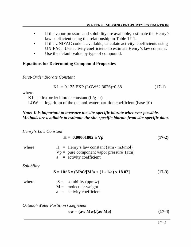
WATER9: MISSING PROPERTY ESTIMATION
17-2
• If the vapor pressure and solubility are available, estimate the Henry’s law coefficient using the relationship in Table 17-1.
• If the UNIFAC code is available, calculate activity coefficients using UNIFAC. Use activity coefficients to estimate Henry’s law constant.
• Use the default value by type of compound.
Equations for Determining Compound Properties
First-Order Biorate Constant
K1 = 0.135 EXP (LOW*2.3026)^0.38 (17-1) where
K1 = first-order biorate constant (L/g-hr) LOW = logarithm of the octanol-water partition coefficient (base 10)
Note: It is important to measure the site-specific biorate whenever possible. Methods are available to estimate the site-specific biorate from site-specific data.
Henry’s Law Constant H = 0.00001802 a Vp (17-2)
where H = Henry’s law constant (atm - m3/mol) Vp = pure component vapor pressure (atm) a = activity coefficient
Solubility S = 10^6 x (M/a)/[M/a + (1 - 1/a) x 18.02] (17-3)
where S = solubility (ppmw) M = molecular weight a = activity coefficient
Octanol-Water Partition Coefficient ow = (aw Mw)/(ao Mo) (17-4)

WATER9: MISSING PROPERTY ESTIMATION
17-3
where ow = octanol-water partition coefficient (g/cc per g/cc) aw = activity coefficient of compound in water mixture ao = activity coefficient of compound in octanol mixture Mw = average molecular weight of water solution (18.02) Mo = average molecular weight of octanol solution (assumed 50% water
content)
Table 17-2. Default Values for Compound Properties Vapor Henry’s lawCompound Molecular Density, pressure, constant,type Code weight g/cc mm Hg atm-m3/mol
General 0 100 1 12 0.0003Aromatic A 100 1.02 4.1 0.0110Biphenyl B 223 1.19 2.9 0.0073Chlorinated C 175 1.41 693.0 10.60Hydrocarbon H 104 0.76 686.0 3.5Inorganic I 75 1.00 0 0Metal M 246 1.65 80.0 0.0073Nitrogen N 194 1.15 188.0 0.1933Oxygenate O 126 0.97 142.0 0.0072Pesticide P 282 1.18 10.0 4,420.0Sulfur S 121 1.26 192.0 0.0280
_________________________________________________________________Henry’s law Diffusion Diffusion
Compound constant, in liquid, in vapor, Biorate, K1,type atm-m3/mol cm2/sec cm2/sec mgVO/g-hr L/g-hr
General 0.0003 0.000008 0.080 15.3 1.0Aromatic 0.0110 0.000008 0.078 31.1 1.88Biphenyl 0.0073 0.000008 0.081 19.0 0.95Chlorinated 10.6 0.000008 0.083 10.76 1.70Hydrocarbon 3.5 0.000008 0.180 15.3 1.0Inorganic 0 0.000008 0.080 0 0Metal 0.0073 0.000008 0.080 0 0Nitrogen 0.1933 0.000012 0.110 9.7 5.02Oxygenate 0.0072 0.000010 0.110 17.56 4.48Pesticide 4,420.0 0.000008 0.080 15.3 2.63Sulfur 0.0280 0.000010 0.100 15.3 2.63
WATER9: MISSING PROPERTY ESTIMATION
17-4
7. If the diffusion coefficient in the liquid is absent, use the correlation in Equation 17-6 to estimate the value.
8. If the diffusion coefficient in the vapor is absent, use the correlation in Equation
17-5 to estimate the value. 9. If the zero-order biorate constant is absent, use the default value by type of
compound. 10. If the first-order biorate constant (K1) is absent, use the first applicable procedure
listed below: • If the octanol-water partition is available, use the OWPC correlation to estimate
K1. • If the UNIFAC code is available, estimate the octanol-water partition
coefficient. Use the OWPC correlation to estimate K1. • A fragment method is alternatively available to estimate K1. • Use the default value by type of compound.
11. If Antoine’s coefficients are absent, then use the first applicable procedure listed below:
• If the boiling point is available, calculate Antoine’s coefficients from the
boiling point and the vapor pressure. • Assume no temperature functionality for the vapor pressure. Calculate
Antoine’s coefficients.
Diffusion Coefficients Correlations were developed to predict the gas phase and liquid phase diffusion coefficients for organic molecules based on empirical correlations using only molecular weight and density. The correlations are used in situations when limited resources preclude the use of more complex correlations, and for situations when only limited compound data are available. The estimated median error of the vapor phase diffusion coefficient correlation is 7%.
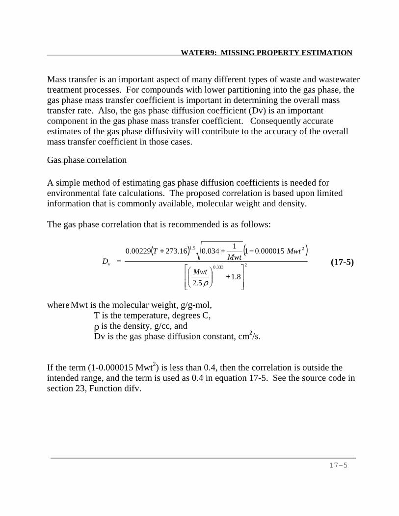
WATER9: MISSING PROPERTY ESTIMATION
17-5
Mass transfer is an important aspect of many different types of waste and wastewater treatment processes. For compounds with lower partitioning into the gas phase, the gas phase mass transfer coefficient is important in determining the overall mass transfer rate. Also, the gas phase diffusion coefficient (Dv) is an important component in the gas phase mass transfer coefficient. Consequently accurate estimates of the gas phase diffusivity will contribute to the accuracy of the overall mass transfer coefficient in those cases.
Gas phase correlation A simple method of estimating gas phase diffusion coefficients is needed for environmental fate calculations. The proposed correlation is based upon limited information that is commonly available, molecular weight and density. The gas phase correlation that is recommended is as follows:
where Mwt is the molecular weight, g/g-mol, T is the temperature, degrees C, ρ is the density, g/cc, and Dv is the gas phase diffusion constant, cm2/s. If the term (1-0.000015 Mwt2) is less than 0.4, then the correlation is outside the intended range, and the term is used as 0.4 in equation 17-5. See the source code in section 23, Function difv.
( ) ( )2333.0
25.1
8.15.2
000015.011034.016.27300229.0
+
−++
ρMwt
MwtMwt
T = Dv (17-5)
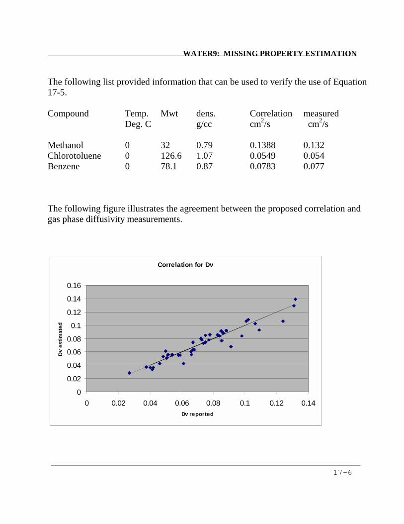
WATER9: MISSING PROPERTY ESTIMATION
17-6
The following list provided information that can be used to verify the use of Equation 17-5. Compound Temp. Mwt dens. Correlation measured Deg. C g/cc cm2/s cm2/s Methanol 0 32 0.79 0.1388 0.132 Chlorotoluene 0 126.6 1.07 0.0549 0.054 Benzene 0 78.1 0.87 0.0783 0.077 The following figure illustrates the agreement between the proposed correlation and gas phase diffusivity measurements.
Correlation for Dv
0
0.02
0.04
0.06
0.08
0.1
0.12
0.14
0.16
0 0.02 0.04 0.06 0.08 0.1 0.12 0.14Dv reported
Dv
estim
ated
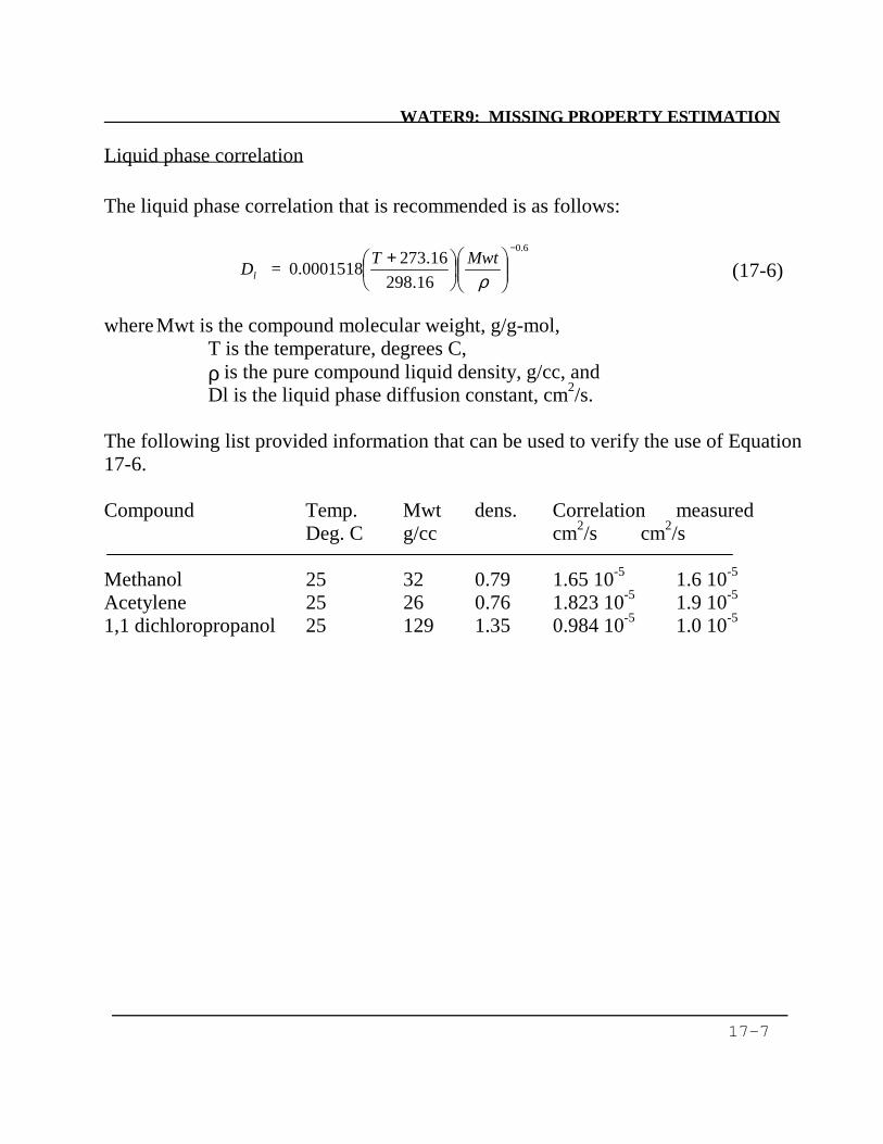
WATER9: MISSING PROPERTY ESTIMATION
17-7
Liquid phase correlation The liquid phase correlation that is recommended is as follows:
where Mwt is the compound molecular weight, g/g-mol, T is the temperature, degrees C, ρ is the pure compound liquid density, g/cc, and Dl is the liquid phase diffusion constant, cm2/s. The following list provided information that can be used to verify the use of Equation 17-6. Compound Temp. Mwt dens. Correlation measured Deg. C g/cc cm2/s cm2/s Methanol 25 32 0.79 1.65 10-5 1.6 10-5 Acetylene 25 26 0.76 1.823 10-5 1.9 10-5 1,1 dichloropropanol 25 129 1.35 0.984 10-5 1.0 10-5
6.0
16.29816.2730001518.0
−
+ρ
MwtT = Dl (17-6)

WATER9: SMILES DATA BASE
18-1
18. SMILES DATA BASE
An extensive compound data base, SMILECAS.mdb is included with the WATER9 distribution package. There are 105,355 records (compounds) with the name of the compound, the CAS number, and a SMILES string. The SMILES string contains compound structural information. WATER9 can search the SMILES data base and extract compound structural information from the SMILES string of the compound in the data base. A translation file smilesrip.txt contains information that WATER9 uses to interpret the information in the SMILES string.
The basic steps used to use the SMILECAS data base are the following:
1. locate the compound of interest, by one of the following methods a. Search by CAS number, b. Search by compound name or part of name, or c. Search by some part of the SMILES string.
2. Decompose the structural information into fragment information a. Automatic WATER9 defragmentation b. Manual fragment identification c. Other method (not available now)
3. Enter the fragment information into the WATER9 compound data base for the compound of interest.
4. Use WATER9 compound property estimation procedures with known compound properties to estimate the needed compound properties.
To use WATER9 in the preceding steps, use the following steps:
1. Open the Multiple Compound Selection Form. Use [Ctrl]C or [Waste][Add compounds to list] to open the form.
2. Enter the CAS number in the box with the label [CAS number]. 3. Press the [CAS lookup SMILES] button to locate the compound. 4. Press the [Calculate UNIFAC, put] button to defragment the compound. 5. The number of fragments and the fragment types are then presented on the
form. Record the results for future use.
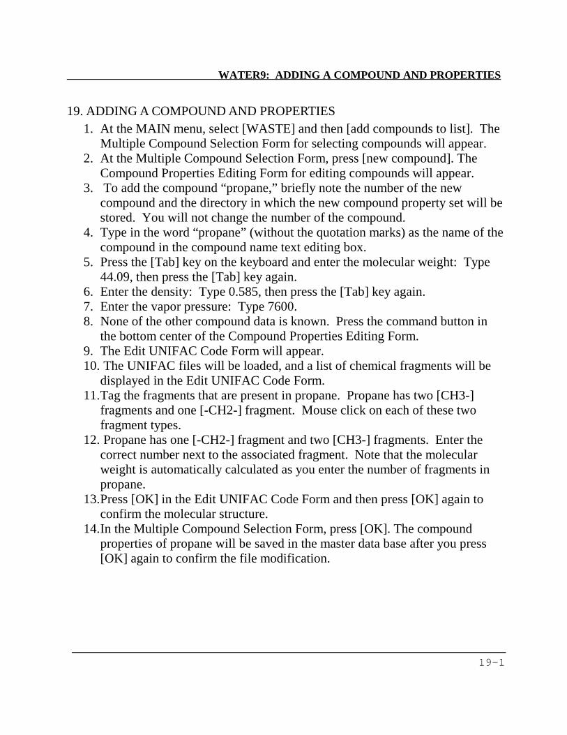
WATER9: ADDING A COMPOUND AND PROPERTIES
19-1
19. ADDING A COMPOUND AND PROPERTIES 1. At the MAIN menu, select [WASTE] and then [add compounds to list]. The
Multiple Compound Selection Form for selecting compounds will appear. 2. At the Multiple Compound Selection Form, press [new compound]. The
Compound Properties Editing Form for editing compounds will appear. 3. To add the compound “propane,” briefly note the number of the new
compound and the directory in which the new compound property set will be stored. You will not change the number of the compound.
4. Type in the word “propane” (without the quotation marks) as the name of the compound in the compound name text editing box.
5. Press the [Tab] key on the keyboard and enter the molecular weight: Type 44.09, then press the [Tab] key again.
6. Enter the density: Type 0.585, then press the [Tab] key again. 7. Enter the vapor pressure: Type 7600. 8. None of the other compound data is known. Press the command button in
the bottom center of the Compound Properties Editing Form. 9. The Edit UNIFAC Code Form will appear. 10. The UNIFAC files will be loaded, and a list of chemical fragments will be
displayed in the Edit UNIFAC Code Form. 11. Tag the fragments that are present in propane. Propane has two [CH3-]
fragments and one [-CH2-] fragment. Mouse click on each of these two fragment types.
12. Propane has one [-CH2-] fragment and two [CH3-] fragments. Enter the correct number next to the associated fragment. Note that the molecular weight is automatically calculated as you enter the number of fragments in propane.
13. Press [OK] in the Edit UNIFAC Code Form and then press [OK] again to confirm the molecular structure.
14. In the Multiple Compound Selection Form, press [OK]. The compound properties of propane will be saved in the master data base after you press [OK] again to confirm the file modification.
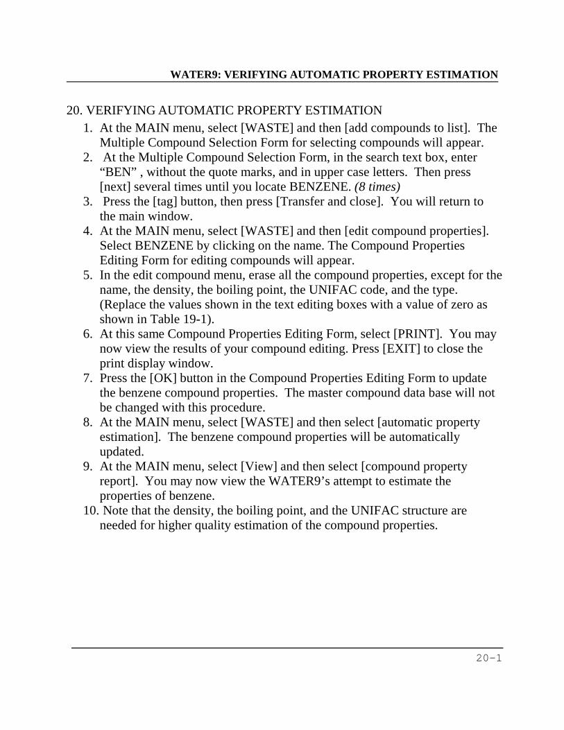
WATER9: VERIFYING AUTOMATIC PROPERTY ESTIMATION
20-1
20. VERIFYING AUTOMATIC PROPERTY ESTIMATION 1. At the MAIN menu, select [WASTE] and then [add compounds to list]. The
Multiple Compound Selection Form for selecting compounds will appear. 2. At the Multiple Compound Selection Form, in the search text box, enter
“BEN” , without the quote marks, and in upper case letters. Then press [next] several times until you locate BENZENE. (8 times)
3. Press the [tag] button, then press [Transfer and close]. You will return to the main window.
4. At the MAIN menu, select [WASTE] and then [edit compound properties]. Select BENZENE by clicking on the name. The Compound Properties Editing Form for editing compounds will appear.
5. In the edit compound menu, erase all the compound properties, except for the name, the density, the boiling point, the UNIFAC code, and the type. (Replace the values shown in the text editing boxes with a value of zero as shown in Table 19-1).
6. At this same Compound Properties Editing Form, select [PRINT]. You may now view the results of your compound editing. Press [EXIT] to close the print display window.
7. Press the [OK] button in the Compound Properties Editing Form to update the benzene compound properties. The master compound data base will not be changed with this procedure.
8. At the MAIN menu, select [WASTE] and then select [automatic property estimation]. The benzene compound properties will be automatically updated.
9. At the MAIN menu, select [View] and then select [compound property report]. You may now view the WATER9’s attempt to estimate the properties of benzene.
10. Note that the density, the boiling point, and the UNIFAC structure are needed for higher quality estimation of the compound properties.

WATER9: VERIFYING AUTOMATIC PROPERTY ESTIMATION
20-2
Table 19-1. Compound Properties for Benzene with Old and New Values Property Old value New value _________________________ ___________ __________ Molecular weight 78.11 0 Vapor pressure 95.2 0 Henry’s law constant 308.32 0 Liquid diffusion coefficient 0.0000102 0 Gas diffusion coefficient 0.088 0 Temperature coefficient a 6.905048 0 Temperature coefficient b 1211.03 0 Temperature coefficient c 220.7996 0 Log octanol-water partition 2.15 0 Biorate Kmax 19.1 0 Monod K1 1.4 0 Characterization code A8 A8 Solubility in water 1780 0

WATER9: VERIFYING AUTOMATIC PROPERTY ESTIMATION
20-3
Table 19-2. Compound Properties for Benzene with Data Base and Reconstructed values
Property Data base value Reconstructed value ___________________ __________ ________________ Molecular weight 78.11 78.12 Vapor pressure 95.2 101.515 Henry’s law constant 308.34 322.2 Liquid *diffusion coefficient 0.0000102 0.0000102 Gas diffusion coefficient 0.088 0.0894 Temperature coefficient a 6.905048 6.839903 Temperature coefficient b 1211.033 1203.786 Temperature coefficient c 220.7996 224.06 Log octanol-water partition 2.15 2.1635 Biorate Kmax 19.1 31.1 Monod K1 1.4 0.896 Characterization code A8 A8 Solubility in water 1780 1799.097

WATER9: EXAMPLE OF PRINTING A REPORT
21-1
21. EXAMPLE OF PRINTING A REPORT 1. At the MAIN menu, select [FILE] and then [Load Project]. A compound name
dialogue box will appear. 2. Load the project file [a print example]. A warning notice will appear in the
center of the screen. 3. Press the [OK] button, confirming that you wish to load the files. 4. Press the [Update] button on the right of the main program window. Observe
the convergence. 5. Mouse click the blue dot under the button under the activated sludge unit. A
small dialogue box will appear. Mouse click the [view] button. 6. Mouse click [print] to print the report.

WATER9: EXAMPLE OF PRINTING A REPORT
21-2
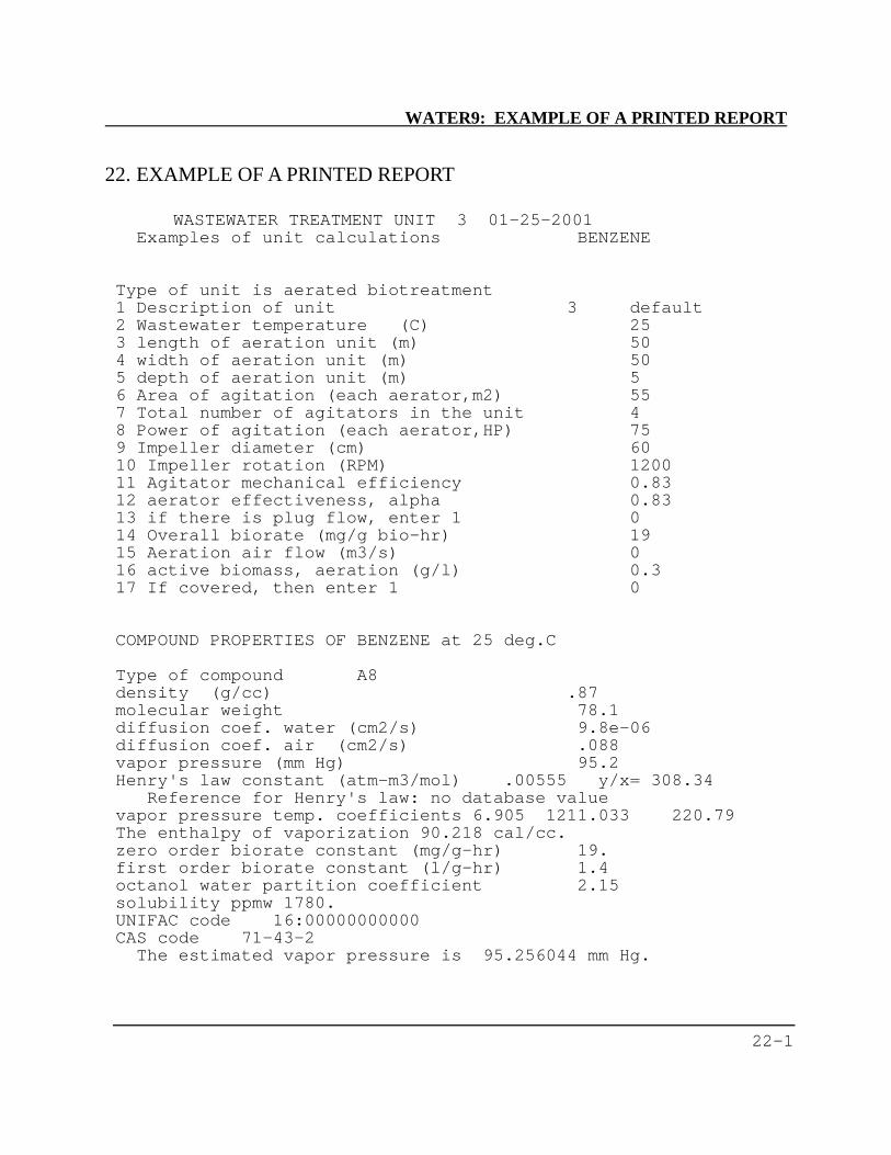
WATER9: EXAMPLE OF A PRINTED REPORT
22-1
22. EXAMPLE OF A PRINTED REPORT
WASTEWATER TREATMENT UNIT 3 01-25-2001Examples of unit calculations BENZENE
Type of unit is aerated biotreatment1 Description of unit 3 default2 Wastewater temperature (C) 253 length of aeration unit (m) 504 width of aeration unit (m) 505 depth of aeration unit (m) 56 Area of agitation (each aerator,m2) 557 Total number of agitators in the unit 48 Power of agitation (each aerator,HP) 759 Impeller diameter (cm) 6010 Impeller rotation (RPM) 120011 Agitator mechanical efficiency 0.8312 aerator effectiveness, alpha 0.8313 if there is plug flow, enter 1 014 Overall biorate (mg/g bio-hr) 1915 Aeration air flow (m3/s) 016 active biomass, aeration (g/l) 0.317 If covered, then enter 1 0
COMPOUND PROPERTIES OF BENZENE at 25 deg.C
Type of compound A8density (g/cc) .87molecular weight 78.1diffusion coef. water (cm2/s) 9.8e-06diffusion coef. air (cm2/s) .088vapor pressure (mm Hg) 95.2Henry's law constant (atm-m3/mol) .00555 y/x= 308.34
Reference for Henry's law: no database valuevapor pressure temp. coefficients 6.905 1211.033 220.79The enthalpy of vaporization 90.218 cal/cc.zero order biorate constant (mg/g-hr) 19.first order biorate constant (l/g-hr) 1.4octanol water partition coefficient 2.15solubility ppmw 1780.UNIFAC code 16:00000000000CAS code 71-43-2
The estimated vapor pressure is 95.256044 mm Hg.
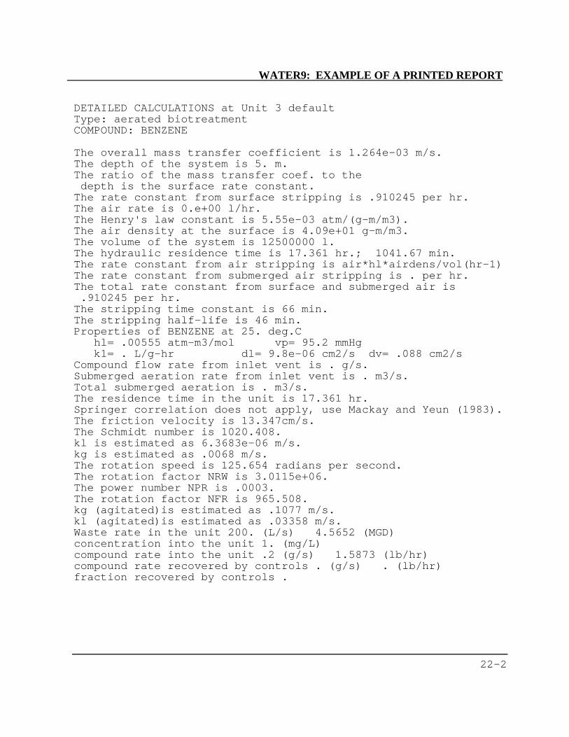
WATER9: EXAMPLE OF A PRINTED REPORT
22-2
DETAILED CALCULATIONS at Unit 3 defaultType: aerated biotreatmentCOMPOUND: BENZENE
The overall mass transfer coefficient is 1.264e-03 m/s.The depth of the system is 5. m.The ratio of the mass transfer coef. to thedepth is the surface rate constant.The rate constant from surface stripping is .910245 per hr.The air rate is 0.e+00 l/hr.The Henry's law constant is 5.55e-03 atm/(g-m/m3).The air density at the surface is 4.09e+01 g-m/m3.The volume of the system is 12500000 l.The hydraulic residence time is 17.361 hr.; 1041.67 min.The rate constant from air stripping is air*hl*airdens/vol(hr-1)The rate constant from submerged air stripping is . per hr.The total rate constant from surface and submerged air is.910245 per hr.The stripping time constant is 66 min.The stripping half-life is 46 min.Properties of BENZENE at 25. deg.C
hl= .00555 atm-m3/mol vp= 95.2 mmHgk1= . L/g-hr dl= 9.8e-06 cm2/s dv= .088 cm2/s
Compound flow rate from inlet vent is . g/s.Submerged aeration rate from inlet vent is . m3/s.Total submerged aeration is . m3/s.The residence time in the unit is 17.361 hr.Springer correlation does not apply, use Mackay and Yeun (1983).The friction velocity is 13.347cm/s.The Schmidt number is 1020.408.kl is estimated as 6.3683e-06 m/s.kg is estimated as .0068 m/s.The rotation speed is 125.654 radians per second.The rotation factor NRW is 3.0115e+06.The power number NPR is .0003.The rotation factor NFR is 965.508.kg (agitated)is estimated as .1077 m/s.kl (agitated)is estimated as .03358 m/s.Waste rate in the unit 200. (L/s) 4.5652 (MGD)concentration into the unit 1. (mg/L)compound rate into the unit .2 (g/s) 1.5873 (lb/hr)compound rate recovered by controls . (g/s) . (lb/hr)fraction recovered by controls .
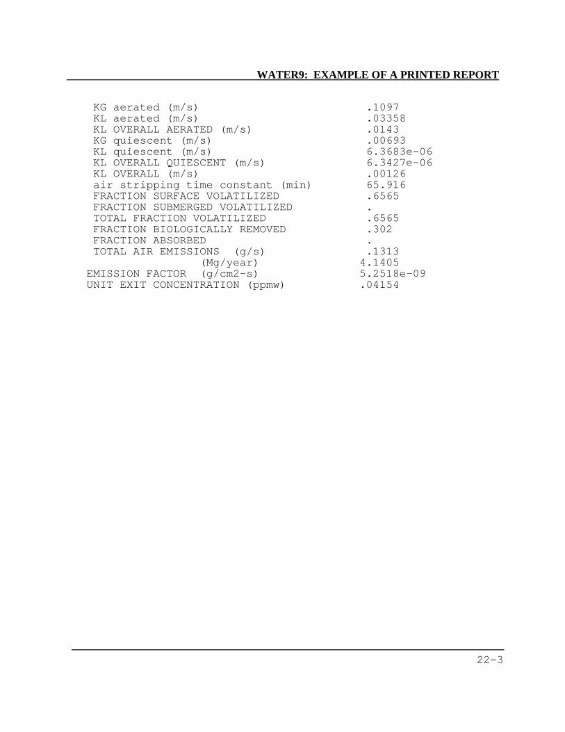
WATER9: EXAMPLE OF A PRINTED REPORT
22-3
KG aerated (m/s) .1097KL aerated (m/s) .03358KL OVERALL AERATED (m/s) .0143KG quiescent (m/s) .00693KL quiescent (m/s) 6.3683e-06KL OVERALL QUIESCENT (m/s) 6.3427e-06KL OVERALL (m/s) .00126air stripping time constant (min) 65.916FRACTION SURFACE VOLATILIZED .6565FRACTION SUBMERGED VOLATILIZED .TOTAL FRACTION VOLATILIZED .6565FRACTION BIOLOGICALLY REMOVED .302FRACTION ABSORBED .TOTAL AIR EMISSIONS (g/s) .1313
(Mg/year) 4.1405EMISSION FACTOR (g/cm2-s) 5.2518e-09UNIT EXIT CONCENTRATION (ppmw) .04154
WATER9: SOURCE CODE
23-1
23. SOURCE CODE
The source code presented in this section is written in Microsoft’s VisualBasic language. Because the program is compiled, the source code is presented so that a user can duplicate the calculations and compare the calculation procedures to the equations presented in the report “Air Emissions Models...”.* This section is not intended to describe the basis of the calculations that are performed by the program or to provide a general discussion; the user should consult Chapter 4.0 in the report “Air Emissions Models...” instead for such information. Table 22-1 presents a cross-reference of the location of the sample calculations for the various units in WATER9. Section 25 presents sample calculations for those wastewater units not included in the report “Air Emissions Models...”.
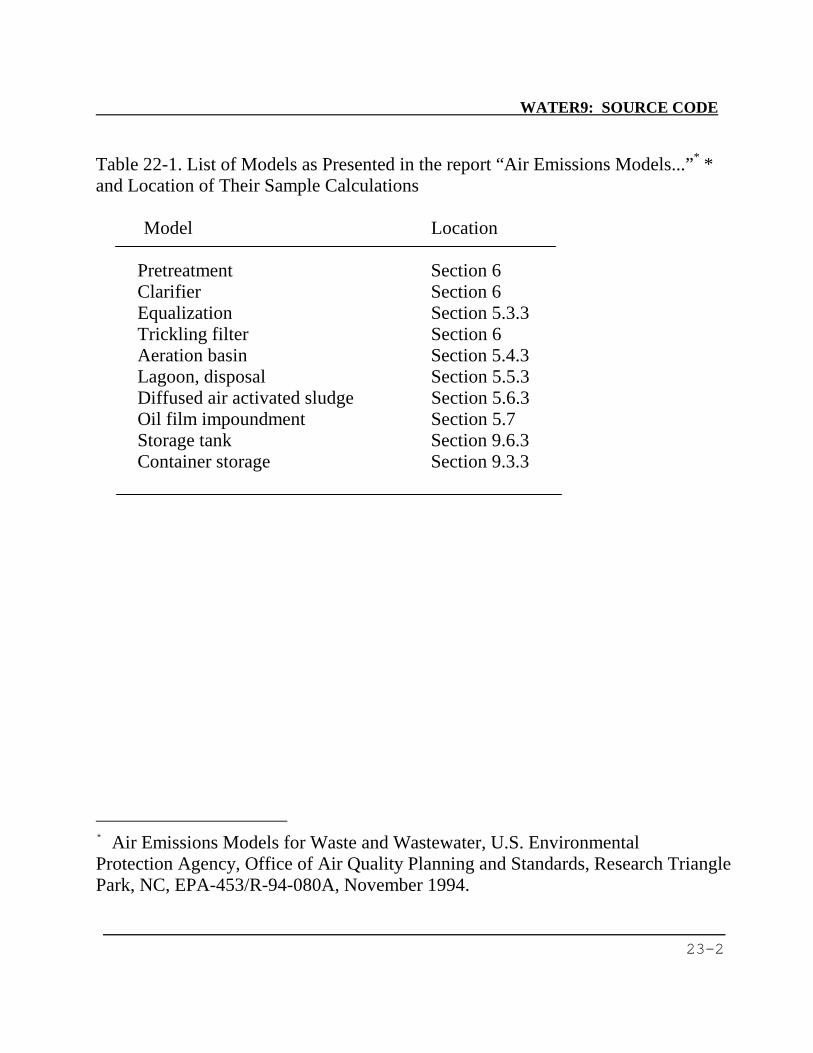
WATER9: SOURCE CODE
23-2
Table 22-1. List of Models as Presented in the report “Air Emissions Models...”* * and Location of Their Sample Calculations Model Location Pretreatment Section 6 Clarifier Section 6 Equalization Section 5.3.3 Trickling filter Section 6 Aeration basin Section 5.4.3 Lagoon, disposal Section 5.5.3 Diffused air activated sludge Section 5.6.3 Oil film impoundment Section 5.7 Storage tank Section 9.6.3 Container storage Section 9.3.3
* Air Emissions Models for Waste and Wastewater, U.S. Environmental Protection Agency, Office of Air Quality Planning and Standards, Research Triangle Park, NC, EPA-453/R-94-080A, November 1994.

WATER9: SOURCE CODE
23-3
Sub Antoines(t1, v1, t2, v2, t3, v3, a, bb, c)If v3 > 0 Thenc = 1 / ((Log(v3 / v2) / Log(v2 / v1) * (t2 - t1) / (t3 - t2) - 1) / (t3 -
t1)) - t3Else: c = 273.16 ' default for c ln(vp)= A exp(B/T(K))End IfIf v1 > 0 And v2 > 0 And Abs(t2 - t1) > 0 Then
bb = Log(v2 / v1) / 2.3026 / (t2 - t1) * (t1 + c) * (t2 + c)a = Log(v1) / 2.3026 + bb / (t1 + c)
ElseIf v1 > 0 Thenbb = 0: a = Log(v1) / 2.3026: c = 0
Else: a = 0: bb = 0: c = 0End If
End Sub
Sub AERATED(nt%)'calculates aerated impoundment fate'_______ input variables___________
Call sets8(nt%, n%, ci, v, q, T)Call Tcorr(k1, vmax, dl, dv, vp, Hl, T, nt%)
Length = asgn8(3) * 100 ' cmta = Length * asgn8(4) / 100 'Total area m2le(nt%).AREA = ta
depth = asgn8(5) * 100 ' cm
If L(nt%).typ = 30 Then 'diffused air sludgefragi = asgn8(6)frqu = asgn8(7)
Elseaag = asgn8(6) ' m2na = asgn8(7)
power = asgn8(8) ' hpdia = asgn8(9) ' cmRPM = asgn8(10)eff = asgn8(11)
alpha = asgn8(12)End Ifplugflow = asgn8(13) ' =1 if plug flow
bioavg = asgn8(14) ' mg/g-bio-hrxb = asgn8(16) ' g/l biomass
controlf = 0
If L(nt%).typ = 38 Thencontrolf = asgn8(18)
End IfairMps = asgn8(15)updateventin nt%, plugflow, ci, q, ta * asgn8(5) * n%, airMps, vairair = airMps * 1000 * 3600 'Diffused air l/hr
' submerged air independent of cover air' submerged air at equilibrium' cover air may or may not be at equilibrium
volpump = asgn8(18) * na 'm3/s from aeratorscovern = asgn8(17)If covern > 0 And covern <> 1 Then 'specified cover vent rate

WATER9: SOURCE CODE
23-4
'm3/m2 surface per secondcoverair = covern * 1000 * 3600 * ta 'L/hrcover% = 1
ElseIf covern = 1 Then '=1 for cover with no coveraircover% = 1: coverair = 0
ElseIf covern < 0 Then 'negative cover for control efficiencycontrolf = -covern: If controlf > 1 Then controlf = 1cover% = 1
Elsecover% = 0
End IfIf n% = 0 Or q = 0 Then Exit Sub ' no sourceql = q * 1000 * 3600 / n% ' L/hr per unitIf showprint = 1 Then
meanrtime = asgn8(5) * asgn8(3) * asgn8(4) * 1000 / qlppprnt "The residence time in the unit is " + FORMP(meanrtime) + " hr."If cover% = 1 Then
ppprnt "The aerated unit has a cover."If controlf > 0 Then ppprnt "The control efficiency of the vent is "
+ FORMP(controlf) + "."ppprnt "The vent flow rate is " + FORMP(asgn8(15)) + " m3/s."Call printprop2(k1, vmax, dl, dv, vp, Hl, T)
End IfEnd If'___ calculates overall mass transfer coef.
If L(nt%).typ = 30 Then 'diffused air biotreatmentareaagit = ta * fragiareaQuies = ta * frquta = areaagit + areaQuiesna = Int(areaagit / 23): If na < 1 Then na = 1aag = ta / nako = KAC8(Length, depth, 1200, 60, dv, 15, 0.85, 0.86, aag, na, dl, Hl *
55555, ta)Else
If eff < 0.01 Then eff = 0.01ko = KAC8(Length, depth, RPM, dia, dv, power, eff, alpha, aag, na, dl, Hl *
55555, ta)End Ifairdens = 1 / 0.0224 * 273 / (273 + T) ' g-m/m3vol = depth * ta * 10 ' volume of impoundment, lrtime = vol / ql ' residence time, hrIf volpump > 0 Then pumptime = vol / volpump / 1000 / 60 'minIf cover% = 1 Then
If coverair = 0 Thenko = 1E-20: For i = 172 To 177: ASGN2(i) = ko: Nextkair = ko / depth * 100 * 3600 ' hr-1
Else'transfer from surfacekair = ko / depth * 100 * 3600 ' hr-1'equilibrium limit in cover airkcover = coverair * Hl * airdens / vol ' hr-1' if greater than equilibrium limit, use equilibrium limitIf kcover < kair Then kair = kcover
End IfElse
controlf = 0
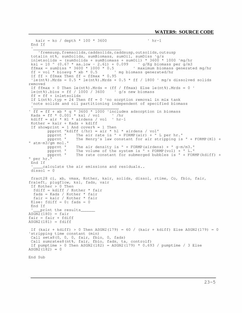
WATER9: SOURCE CODE
23-5
kair = ko / depth * 100 * 3600 ' hr-1End If'_____________________________________
'fremsusp,fremsolids,caddsolids,caddsusp,outsolids,outsusptotalin nt%, sumSolids, sumBiomass, sumOil, sumDiss 'g/sinletsolids = (sumSolids + sumBiomass + sumOil) * 3600 * 1000 'mg/hrksl = 10 ^ (0.67 * aa.low - 2.61) + 0.099 ' g/Kg biomass per g/m3ffmax = sumDiss * 3600 * 1000 * 0.5 ' maximum biomass generated mg/hrff = vol * bioavg * xb * 0.5 ' mg biomass generated/hrIf ff > ffmax Then ff = ffmax * 0.95'le(nt%).Mrds = 0.5 * le(nt%).Mrds + 0.5 * ff / 1800 ' mg/s dissolved solids
removedIf ffmax > 0 Then le(nt%).Mrds = (ff / ffmax) Else le(nt%).Mrds = 0 'le(nt%).bios = ff / 1000 / 3600 ' g/s new biomassff = ff + inletsolidsIf L(nt%).typ = 24 Then ff = 0 'no sorption removal in mix tank'note solids and oil partitioning independent of specified biomass'____________________________________
' ff = ff + xb * q * 3600 * 1000 'includes adsorption in biomassKads = ff * 0.001 * ksl / vol ' /hrkdiff = air * Hl * airdens / vol ' hr-1Kother = kair + Kads + kdiffIf showprint = 1 And cover% = 1 Then
ppprnt "kdiff (/hr) = air * hl * airdens / vol"ppprnt " The air rate is " + FORMP(air) + " L per hr."ppprnt " The Henry's law constant for air stripping is " + FORMP(Hl) +
" atm-m3/gm mol."ppprnt " The air density is " + FORMP(airdens) + " g-m/m3."ppprnt " The volume of the system is " + FORMP(vol) + " L."ppprnt " The rate constant for submerged bubbles is " + FORMP(kdiff) +
" per hr."End If'____calculate the air emissions and residuals..dissol = 0
fract28 ci, xb, vmax, Kother, kair, solids, dissol, rtime, Co, fbio, fair,fraleft, plugflow, ksl, fads, vairIf Kother > 0 Thenfdiff = kdiff / Kother * fairfads = Kads / Kother * fairfair = kair / Kother * fair
Else: fdiff = 0: fads = 0End If'___print the results______
ASGN2(180) = fairfair = fair + fdiffASGN2(181) = fdiff
If (kair + kdiff) > 0 Then ASGN2(179) = 60 / (kair + kdiff) Else ASGN2(179) = 0'stripping time constant (min)Call setx8(0, 0, 0, fair, fbio, 0, fads)Call sumrates8(nt%, fair, fbio, fads, ta, controlf)If pumptime > 0 Then ASGN2(182) = ASGN2(179) * 0.693 / pumptime / 3 Else
ASGN2(182) = 0
End Sub

WATER9: SOURCE CODE
23-6
Sub APISEPARATOR(nt%)Call sets8(nt%, n%, ci, v, q, T)If n% = 0 Or q = 0 Then Exit Subareaenter = asgn8(3) 'm2areaoil = asgn8(4) 'm2fractoil = asgn8(5) 'fraction of separation surface covered with oiloilfract = asgn8(6) / 100 'fraction oil in total wastedensoil = asgn8(7) 'g/cm3mwtoil = asgn8(8)drop = asgn8(9) ' cmwidthFall = asgn8(10) ' mremoval = asgn8(11) ' fraction of oil removed by separatorta = areaenter + areaoille(nt%).AREA = tadia = Sqr(areaenter * 4 / 3.14) 'width mASGN2(107) = diatotalin nt%, sumSolids, sumBiomass, sumOil, sumDiss 'g/sCall Tcorr(k1, vmax, dl, dv, vp, Hl, T, nt%)If oilfract = 0 Then
Call fractionoil(oilfract, owpc, owr, frinoil, nt%)Else
Call fractionoil(oilfract, owpc, owr, frinoil, 0) 'use specificationEnd IfIf showprint = 1 Then ppprnt "The oil corrected aqueous HL is " + Format$(Hl
* (1 - frinoil) * 55555, "#.###e+00 (y/x)")
'____entrance zone______kg = KGC8(v, dia * 100, dv, 2) ' Gmol/cc-seckl = KLC8(v, 180, dl, T, 6, 0, 1) ' Gmol/cc-secko = 1 / (1 / kl + 1 / Hl / (1 - frinoil) / 55555 / kg)Mtr = ko * 0.18 * areaenter * n% / qfrEnt = 1 - Exp(-Mtr)
'____oil covered separation zone______Keq = vp * 0.0012 * mwtoil / densoil / 28.8 / 760k = Keq * kg * 240 ' m/sxmtr = k * areaoil * fractoil * owpc * n% / q'____water covered separation zone______mtr2 = ko * 0.18 * areaoil * (1 - fractoil) * n% / qfroil = 1 - Exp(-xmtr - mtr2)frabs = (1 - frEnt) * (1 - froil) * frinoil * removal
'____waterfall exit zone______wkg = KGC8(v, widthFall * 100, dv, 6) ' gmol/cm2-secCall WEIR(widthFall, q / n%, drop / 100, frwf, wkl, dl, 0)wkl = wkl / 0.18 'g m/cm-swko = 1 / (1 / wkl + 1 / Hl / 55555 / wkg)AREA = widthFall * drop / 100 'm2Mtr = wko * 0.18 * AREA / q * n%frwf = 1 - Exp(-Mtr)
'__print results_______Call setx1(kg / 0.00409, kl * 0.18, ko * 0.18, frEnt, doil, 0, froil, frwf,
55555 * Hl * (1 - frinoil), frinoil)fair = frEnt + (1 - frEnt) * froil + (1 - frEnt) * (1 - froil) * (1 -
frinoil) * frwfASGN2(182) = fairASGN2(183) = frabsCall sumrates8(nt%, fair, 0, frabs, ta, 0)
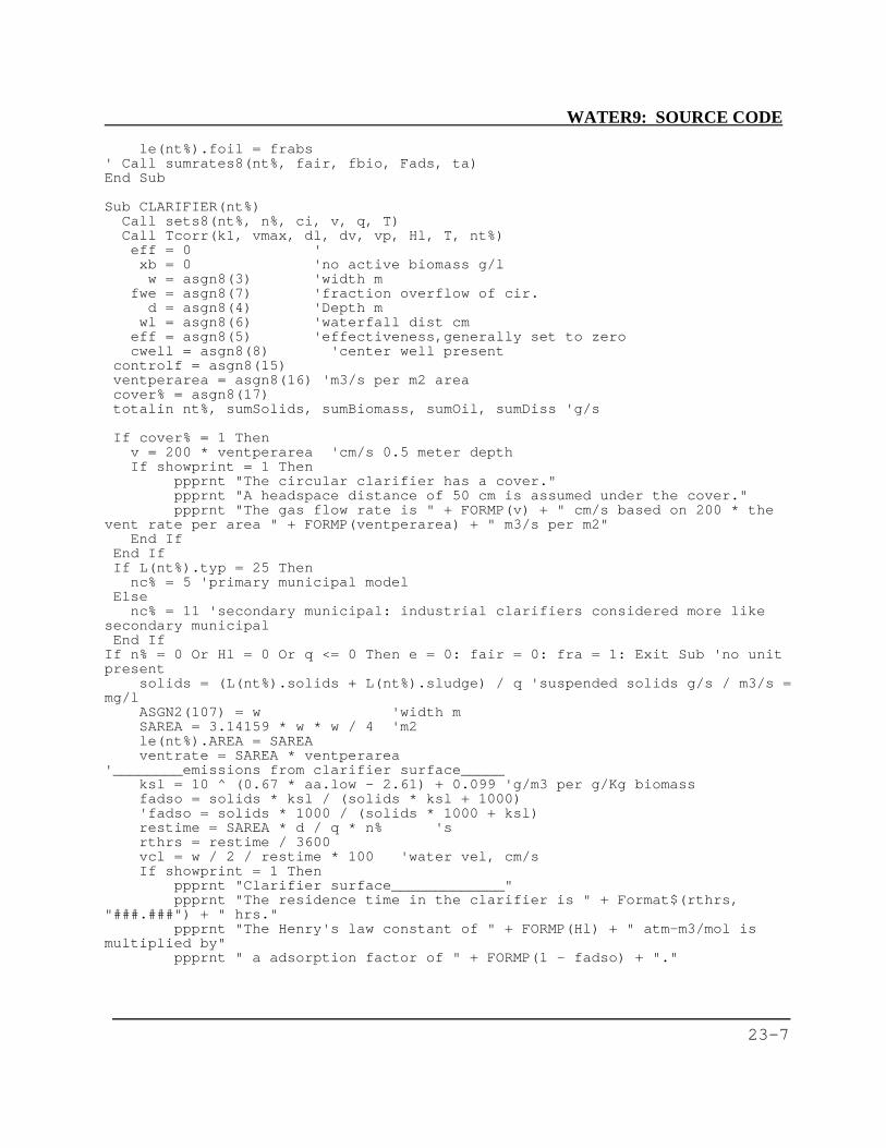
WATER9: SOURCE CODE
23-7
le(nt%).foil = frabs' Call sumrates8(nt%, fair, fbio, Fads, ta)End Sub
Sub CLARIFIER(nt%)Call sets8(nt%, n%, ci, v, q, T)Call Tcorr(k1, vmax, dl, dv, vp, Hl, T, nt%)eff = 0 'xb = 0 'no active biomass g/lw = asgn8(3) 'width m
fwe = asgn8(7) 'fraction overflow of cir.d = asgn8(4) 'Depth m
wl = asgn8(6) 'waterfall dist cmeff = asgn8(5) 'effectiveness,generally set to zerocwell = asgn8(8) 'center well present
controlf = asgn8(15)ventperarea = asgn8(16) 'm3/s per m2 areacover% = asgn8(17)totalin nt%, sumSolids, sumBiomass, sumOil, sumDiss 'g/s
If cover% = 1 Thenv = 200 * ventperarea 'cm/s 0.5 meter depthIf showprint = 1 Then
ppprnt "The circular clarifier has a cover."ppprnt "A headspace distance of 50 cm is assumed under the cover."ppprnt "The gas flow rate is " + FORMP(v) + " cm/s based on 200 * the
vent rate per area " + FORMP(ventperarea) + " m3/s per m2"End If
End IfIf L(nt%).typ = 25 Then
nc% = 5 'primary municipal modelElse
nc% = 11 'secondary municipal: industrial clarifiers considered more likesecondary municipalEnd If
If n% = 0 Or Hl = 0 Or q <= 0 Then e = 0: fair = 0: fra = 1: Exit Sub 'no unitpresent
solids = (L(nt%).solids + L(nt%).sludge) / q 'suspended solids g/s / m3/s =mg/l
ASGN2(107) = w 'width mSAREA = 3.14159 * w * w / 4 'm2le(nt%).AREA = SAREAventrate = SAREA * ventperarea
'________emissions from clarifier surface_____ksl = 10 ^ (0.67 * aa.low - 2.61) + 0.099 'g/m3 per g/Kg biomassfadso = solids * ksl / (solids * ksl + 1000)'fadso = solids * 1000 / (solids * 1000 + ksl)restime = SAREA * d / q * n% 'srthrs = restime / 3600vcl = w / 2 / restime * 100 'water vel, cm/sIf showprint = 1 Then
ppprnt "Clarifier surface_____________"ppprnt "The residence time in the clarifier is " + Format$(rthrs,
"###.###") + " hrs."ppprnt "The Henry's law constant of " + FORMP(Hl) + " atm-m3/mol is
multiplied by"ppprnt " a adsorption factor of " + FORMP(1 - fadso) + "."

WATER9: SOURCE CODE
23-8
ppprnt "The adsorption corrected aqueous HL is " + Format$(Hl * (1 -fadso) * 55555, "#.###e+00 (y/x)")
ppprnt "The gas phase mass transfer is estimated using correlation 3,MacKay (1983)."
End Ifskg = KGC8(v, w * 100, dv, 3) 'gm/c2-sVclc = vcl * 10 'corrects for flow distributionIf cwell > 0.01 Then flowfactor = 0.13 Else flowfactor = 0.1skl = KLC8(Vclc, d * 100, dl, q / n% * 10000 / w * 2, 7, 0, flowfactor)
'gm/c2-sIf skl > 0 And Hl > 0 And skg > 0 Then sko = 1 / (1 / skl + 1 / (Hl * (1 -
fadso)) / 55555 / skg) Else skl = 0 'gm/c2-sMtr = sko * 0.18 / d * restimesfair = 1 - Exp(-Mtr)If cover% = 1 And ventrate = 0 Then sfair = 0If eff > 0 Then
fads = eff * fadso ' corrects for settling losses,equil.solids = solids * (1 - eff) ' after settling
Elsefads = fadso
End IfIf showprint = 1 Then
ppprnt "Gas phase mass transfer " + FORMP(skg) + " g mol/ cm2-s."ppprnt " The flow of water is " + FORMP(q / n% * 1000) + " cm3/s."ppprnt " The effective flow depth in the clarifier is " + FORMP(d * 10)
+ " cm."ppprnt "Clarifier model liquid phase mass transfer " + FORMP(skl) + " g
mol/ cm2-s."ppprnt "Overall mass transfer " + FORMP(sko) + " g mol/cm2-s."
End If
If showprint = 1 Thenppprnt "Clarifier weir emissions_____________"
End Ifcir = 3.14159 * w * fwe 'circumference, mwkg = KGC8(v, wl, dv, 3) ' gmol/c2-sec '%%%%wl?? width of air flow cmCall WEIR(cir, q / n%, wl / 100, fair, wkl, dl, nc%) 'reference
wkl = wkl / 0.18 'g m/cm-swko = 1 / (1 / wkl + 1 / (Hl * (1 - fadso)) / 55555 / wkg)
AREA = cir * wl / 100 'm2Mtr = wko * 0.18 * AREA / q * n%
wfair = 1 - Exp(-Mtr)
'_____cover effects_______If cover% = 1 Then
If ventrate = 0 Thenwfair = 0: sfair = 0 'mass transfer supressed
Else'-------
airdens = 1 / 0.0224 * 273 / (273 + T) ' g-m/m3koc = (Hl * (1 - fadso) * 55555)air = ventrate 'emitted air m3/sgm = airdens * air 'moles/s gasarear = SAREA 'area m2kor = sko * 0.18 'm/s
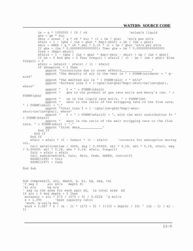
WATER9: SOURCE CODE
23-9
Lm = q * 1000000 / 18 / n% 'moles/s liquidghx = gm * kocskor = arear / q * n% * kor * (1 + Lm / ghx) 'm3/s per m3/ssfair = 1 - (ghx / (Lm + ghx) * Exp(-skor) + Lm / (Lm + ghx))wkor = AREA / q * n% * wko * 0.18 * (1 + Lm / ghx) 'm3/s per m3/sIf ghx < (Lm * 0.000000000000001) Then ghx = Lm * 0.000000000000001fres = (Exp(-skor))wfair2 = 1 - (ghx / (Lm + ghx) * Exp(-wkor - skor) + Lm / (Lm + ghx))If Lm > 0 And ghx > 0 Then frequil = wfair2 / (1 - Lm / (Lm + ghx)) Else
frequil = 0wfair = (wfair2 - sfair) / (1 - sfair)If showprint = 1 Then
ppprnt "Corrections due to cover effects________________"ppprnt "The density of air in the vent is " + FORMP(airdens) + " g-
m/m3"ppprnt "The emitted air is " + FORMP(air) + " m3/s"ppprnt "Surface loss f = 1-(ghx/(Lm+ghx)*Exp(-skor)+Lm/(Lm+ghx)),
where"ppprnt " f = " + FORMP(sfair)ppprnt " ghx is the product of gas rate mol/s and Henry's law, " +
FORMP(ghx)ppprnt " Lm is the liquid rate mol/s, " + FORMP(Lm)ppprnt " skor is the ratio of the stripping rate to the flow rate,
" + FORMP(skor) + "."ppprnt "Total loss f = 1 -(ghx/(Lm+ghx)*Exp(-wkor-
skor)+Lm/(Lm+ghx)), where"ppprnt " f = " + FORMP(wfair2) + ", with the weir contribution f= "
+ FORMP(wfair)ppprnt " wkor is the ratio of the weir stripping rate to the flow
rate, " + FORMP(wkor) + "."ppprnt "Inlet data____________"
End IfEnd If
End Ifwfair = wfair * (1 - fadso) * (1 - sfair) 'corrects for adsorption during
vol.Call setx1(restime / 3600, skg / 0.00409, skl * 0.18, sko * 0.18, sfair, wkg
/ 0.00409, wkl * 0.18, wko * 0.18, wfair, frequil)fair = sfair + wfairCall sumrates8(nt%, fair, fbio, fads, SAREA, controlf)ASGN2(188) = fairASGN2(187) = fads
End Sub
Sub compress(T, air, depth, k, kl, kg, aag, ta)'T deg C air m3/s depth ft'kl m/s kg m/s' aag is the area for each agit m2, ta total area m2If air > 0 And depth > 0 Thenmolesair = air * 273 / (273 + T) / 0.0224 'g mol/sk = 1.395 'heat capacity ratio'work, g-cal/g molwork = 1.987 * k / (k - 1) * (273 + T) * (((33 + depth) / 33) ^ ((k - 1) / k) -
1)

WATER9: SOURCE CODE
23-10
hp = work * molesair * 4.18 / 746' agitator model for air emissionspow = hp: na = 1
Else: pow = 0: na = 0: aag = 0End If
eff = 1: alpha = 0.65kl = KAC8(0, depth * 30.48, 1200, 60, aa.dv, pow, eff, alpha, aag, na, aa.dl, k,
ta)End Sub
Sub CONDVENT(nt%)oilfract = asgn8(2) 'fract oil in cond.temp = asgn8(3) 'temp of the exit venttempventin = asgn8(4)rhvent = asgn8(5) ' fract. actual humiditydirectwater = asgn8(6) 'l/sindirectwater = asgn8(8) 'l/synonin = asgn8(9) 'y noncond in ventgasflow = asgn8(10) 'gmol/syin = asgn8(11) / 1000000 'ppmv > y incooltemp = asgn8(12) 'cooling water
totalMPS = gasflow + directwater * 1000 / 18'___flow rate water in condensate___ywaterin = rhventhumidity8 temp, 1, ywaterout, rhowater 'saturated condensatewaterinMPS = rhvent * gasflowIf asgn8(22) = 1 Then ynonin = 1 - ywaterincompMPS = yin * gasflownonmps = ynonin * gasflow
If ywaterout >= 1 Then ywaterout = 0.9999waterinvent = waterinMPS * 18 / 1000 'l/s water in vapor'assumes total mols=water + noncondnonoutmps = gasflow * ynoninIf ywaterout < ywaterin Then
totaloutventmps = gasflow * ynonin / (1 - ywaterout)wateroutventMPS = totaloutventmps - nonoutmpswateroutvent = wateroutventMPS * 18 / 1000 'l/s water not condensedcondensate = waterinvent - wateroutvent + directwater 'L/s
Elsecondensate = directwatertotaloutventmps = gasflowwateroutventMPS = gasflow * ywaterinwateroutvent = waterinvent
End IfIf gasflow > 0 Thenfractioncondensed = (gasflow - totaloutventmps) / gasflow
Elsefractioncondensed = 0
End IfwateroutcondMPS = condensate * 1000 / 18If condensate > 0 Then
Call Tcorr(k1, vmax, dl, dv, vp, Hl, temp, nt%)vp = vp / 760 'atmCall fractionoil(oilfract, owpc, owr, frinoil, 0)
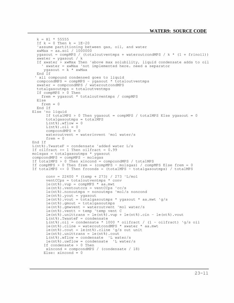
WATER9: SOURCE CODE
23-11
k = Hl * 55555If k = 0 Then k = 1E-20'assume partitioning between gas, oil, and waterxwMax = aa.sol / 1000000ygasout = compMPS / (totaloutventmps + wateroutcondMPS / k * (1 + frinoil))xwater = ygasout / kIf xwater > xwMax Then 'above max solubility, liquid condensate adds to oil
' xwater = xwMax 'not implemented here. need a separatorygasout = k * xwMax
End If' all compound condensed goes to liquidcompcondMPS = compMPS - ygasout * totaloutventmpsxwater = compcondMPS / wateroutcondMPStotalgasoutmps = totaloutventmpsIf compMPS > 0 Then
frem = ygasout * totaloutventmps / compMPSElse
frem = 0End If
Else 'no liquidIf totalMPS > 0 Then ygasout = compMPS / totalMPS Else ygasout = 0totalgasoutmps = totalMPSL(nt%).wflow = 0L(nt%).oil = 0compcondMPS = 0wateroutvent = waterinvent 'mol water/sfrem = 0
End IfL(nt%).TwasteF = condensate 'added water L/sIf oilfract >= 1 Then oilfract = 0.99molsgas = totalgasoutmps * ygasoutcompcondMPS = compMPS - molsgasIf totalMPS > 0 Then xincond = compcondMPS / totalMPSIf compMPS > 0 Then frem = (compMPS - molsgas) / compMPS Else frem = 0If totalMPS <> 0 Then frconds = (totalMPS - totalgasoutmps) / totalMPS
conv = 22400 * (temp + 273) / 273 'L/molventCCps = totaloutventmps * convle(nt%).vup = compMPS * aa.mwtle(nt%).ventoutccs = ventCCps 'cc/sle(nt%).nonoutmps = nonoutmps 'mol/s noncondle(nt%).yout = ygasoutle(nt%).vout = totalgasoutmps * ygasout * aa.mwt 'g/sle(nt%).gmout = totalgasoutmpsle(nt%).gmwvent = wateroutvent 'mol water/sle(nt%).ventt = temp 'temp vent Cle(nt%).unittrans = le(nt%).vup + le(nt%).cin - le(nt%).voutL(nt%).TwasteF = condensateL(nt%).oil = condensate * 1000 * oilfract / (1 - oilfract) 'g/s oille(nt%).cline = wateroutcondMPS * xwater * aa.mwtle(nt%).cout = le(nt%).cline 'g/s out unitle(nt%).unittrans = le(nt%).coutL(nt%).wflow = condensate 'L water/sle(nt%).uwflow = condensate 'L water/s
If condensate > 0 Thenxincond = compcondMPS / (condensate / 18)
Else: xincond = 0
WATER9: SOURCE CODE
23-12
End IfIf showprint = 1 Then
totalmpsin = waterinMPS + compMPS + nonmpsppprnt " The fraction of the water that is condensed is " +
Format(fractioncondensed, "#.######")ppprnt " The inlet gas compound concentration is " + FORMP(yin) + "
mol fraction"ppprnt " The inlet vent rate is " + FORMP(gasflow) + " mol per s"ppprnt " The exit vent rate is " + FORMP(totaloutventmps) + " mol per
s"ppprnt " The exit condensate is " + FORMP(wateroutcondMPS) + " mol per
s"ppprnt " The exit condensate is " + FORMP(condensate) + " L per s"If xwater > 0 Then ppprnt " The exit condensate is " +
FORMP(wateroutcondMPS * xwater * aa.mwt) + " g compound per s"If condensate > 0 Then ppprnt " The condensate concentration is " +
FORMP(le(nt%).cout / condensate) + " weight fract."End If
'tmpsout, gpsout, molwaterout, molnoncoutunit_vent_out nt%, temp, totalgasoutmps, le(nt%).vout, wateroutventMPS, nonmpsIf totalgasoutmps > 0 Then frnon = nonmps / totaloutventmps' 172v 173v 4v 5 6v 7v
178v 179 180Call setx1(le(nt%).yout, xwater, frem, oilfract, frinoil, condensate,
totaloutventmps * 22.4, frnon, fractioncondensed, 0)
findexitvent isect 'also updates flows in vent, airBreak = Break
Exit Sub
End Sub
Sub coolcalcsa8(nt%, twater(), tair(), numbElements, enthalpy())Call sets8(nt%, n%, ci, v, q, tinL)Call Tcorr(k1, vmax, dl, dv, vp, Hl, tinL, nt%)
cpair = 0.25 'cal/g-degCKH20 = 0.014 'btu/ft2-hr-degFMair = 29 'g/molratio = 0.87 '(Nsh/Npr)^.667dvwv = 0.1 'water vapor cm2/sdH = 18000 'cal/mol vaporizationtp = asgn8(12) 'total bed porositycrossdraft = asgn8(14) '1, crossdraft, else packed bedfrr = asgn8(3) 'fraction recyclehumid = asgn8(10) / 100 'Humidity inlet air (fraction sat,)Tina = asgn8(9) 'Temp inlet air Ctlength = asgn8(5) 'length of tower mtheight = asgn8(6) ' thickness of tower packing mtWidth = asgn8(4) ' width of tower packing mIf crossdraft = 1 ThenFLOWx = q / n% / 2 / (1 - frr) 'one side m3/sCAREAM = tWidth * theight 'crossdraft based on side areas
ElseFLOWx = q / n% / (1 - frr) 'm3/sCAREAM = tWidth * tlength
WATER9: SOURCE CODE
23-13
End IfCrossarea = tlength * tWidthQg = asgn8(11) * CAREAM 'air flow m3/sIf Qg = 0 Then Qg = 0.1rtwater = asgn8(8) 'liquid holdup s/mlp = rtwater * FLOWx / CrossareaIf (tp - lp) > 0 Then flood = lp / (tp - lp) Else flood = 0aOa = asgn8(7) / 100 'm2/m3 to cm2/cm3Carea = Crossarea * 10000 'tower cross sect, cm2pd = 6 / aOa * (1 - tp) 'equivalent dia packing cmASGN2(90) = pdpa = tp - lp: If pa < 0 Then pa = 0.01molDensitya = 1 / 0.0224 * 273 / (Tina + 273) 'mol/m3moldensityac = molDensitya * 1000000! 'mol/cm3moldensityL = 1000000! / 18 'mol/m3La = FLOWx * 1000000# / Carea 'cm3/cm2-sGa = Qg * molDensitya / Carea 'gmol/cm2-smol_water_psec = FLOWx * 55555 'mol water/sG = Qg * molDensitya 'mol gas/s
'___water vapor____Scgw = 0.00018 / 0.0011 / dvwvkg = Ga * Scgw ^ -0.666 * 1.1958 * (pd * Ga * 29 / 0.00018 / (1 - pa)) ^ -0.36
'mol/cm2-skgw = kg * moldensityac 'water, cm/sh = cpair * kg * Mair * ratio 'cal/cm2-sec-C'___cooling converg____delH = theight * 100 / numbElements 'cm
' volelement = Carea * delH * pa 'cm3' rtair = volelement / (Qg * 1000000) 'residence sec
consta = aOa * Carea * delH 'cm2 surface/elementconstb = kg * aOa * Carea * delH 'mol transferred/s-elementTmax = Tina: If Tmax < tinL Then Tmax = tinLwetbulb Tina, Tmin, humidIf Tmin > tinL Then Tmin = tinLacc = 1deltstart = Abs(tinL - Tina)Tl = Tinatlo = TlnumIter = 80recycle = asgn8(3)If recycle < 0.1 Then numIter = 20For ii = 1 To numItertspecs = tinL * (1 - recycle) + recycle * tloGoSub estimatetemp 'returns TL<>TinL'converg. criteriaIf Tl > tspecs Then
If acc < 1 Then acc = accIf acc > 0 Then acc = -acc / 2
ElseIf acc > 1 Then acc = accIf acc < 0 Then acc = -acc / 2
End IfTl = tlo + acc 'adjusts temperature at base of towertlo = Tl
WATER9: SOURCE CODE
23-14
NextCall humidity8(TG, 1, ywater, rhowater)ASGN2(279) = Y / ywater * 100
'___compound____Call KLP(pd, La, 0.00001, kl) 'Kl, cm/sCall Kgp8(pd, pa, Ga, kg) 'Kg, cm/sKeq = 40.9 * 0.00554If kl > 0 And kg > 0 Then
KoL = 1 / (1 / kl + 1 / kg / Keq) 'cm/sElse: KoL = 0End IfMtr = KoL * aOa 'cm/s* cm2/cm3* f /sASGN2(91) = klASGN2(92) = kgASGN2(93) = MtrIf Carea > 0 Then Vgas = 1000000 * Qg / Carea Else Vgas = -100 'cm/s
Exit Sub
estimatetemp:
TG = Tinahum = humidCall humidity8(TG, hum, ywater, rhowater)Y = ywatermol_water_psec = FLOWx * 55555 'mol/sG = Qg * molDensitya 'mol/sASGN2(291) = Tlsummass = 0
If crossdraft = 1 Then'assumes one stage crossflow,numbelements stages downsumtempair = 0sumyair = 0sumwatertrans = 0Tl = tspecs 'cools from top downGair = G / numbElementsFor i = 1 To numbElements
Call humidity8(Tl, 1, ye, rhowater)dmdt = (ye - ywater) * constb 'mols/s-elementdmdtmax = (ye - ywater) * GairIf dmdt <> 0 Then dmdt = dmdtmax * (1 - Exp(-dmdt / dmdtmax))yout = (ywater * Gair + dmdt) / (Gair + dmdt)mol_water_psec = mol_water_psec - dmdtdcdtV = dmdt * dH 'cal/s vaporizationDcdtT = h * consta * (Tl - TG) 'cal/s heat transferDcdtTv = dmdt * 18 * cpair * (Tl - TG) 'cal/s warm vapor addeddcdtTmaX = (Tl - TG) * cpair * Gair * MairIf DcdtT <> 0 Then DcdtT = dcdtTmaX * (1 - Exp(-DcdtT / dcdtTmaX))twater(numbElements - i + 1) = Tl 'ASGN2(290 + i)Tl = Tl - (dcdtV + DcdtT) / (mol_water_psec * 18) 'temp liq into elemtairout = TG + (DcdtT + DcdtTv) / (cpair * Gair * Mair) 'temp gas
out of elementtair(numbElements - i + 1) = tairoutsumwatertrans = sumwatertrans + DcdtTvsumtempair = sumtempair + tairoutsummass = summass + dmdtsumyair = sumyair + yout
WATER9: SOURCE CODE
23-15
Next iTG = sumtempair / numbElementsY = sumyair / numbElementstlo = TlTempWaterout = tloTempAirout = TG
ElseFor i = 1 To numbElements
Call humidity8(Tl, 1, ye, rhowater)dmdt = (ye - Y) * constb 'mols/s-elementdmdtmax = (ye - Y) * G
If dmdt <> 0 Then dmdt = dmdtmax * (1 - Exp(-dmdt / dmdtmax))summass = summass + dmdtY = (Y * G + dmdt) / (G + dmdt)mol_water_psec = mol_water_psec + dmdtG = G + dmdt
dcdtV = dmdt * dH 'cal/s vaporizationDcdtT = h * consta * (Tl - TG) 'cal/s heat transferDcdtTv = dmdt * 18 * cpair * (Tl - TG) 'cal/s warm vapor addeddcdtTmaX = (Tl - TG) * cpair * G * MairIf DcdtT <> 0 Then DcdtT = dcdtTmaX * (1 - Exp(-DcdtT / dcdtTmaX))twater(i) = Tl 'ASGN2(290 + i)Tl = Tl + (dcdtV + DcdtT) / (mol_water_psec * 18) 'temp liq into elemTG = TG + (DcdtT + DcdtTv) / (cpair * G * Mair) 'temp gas out of element
If Tl > Tmax + 5 Then Tl = Tmax + 5 ' modified 2-17-00 limit temperature attop
If Tl < Tmin Then Tl = TminIf TG > Tmax Then TG = TmaxIf TG < Tmin Then TG = Tmintair(i) = TG 'ASGN2(280 + i)
Next iTempWaterout = twater(1)TempAirout = tair(numbElements) 'ASGN2(290)
End Ifenthalpy(1) = summass * dHenthalpy(2) = TempAiroutenthalpy(3) = summassdelenthalpyair = (TempAirout - Tina) * cpair * G * Mairdelenthalpywater = (tspecs - TempWaterout) * 1 * mol_water_psec * 18enthalpy(4) = delenthalpyairenthalpy(5) = delenthalpywaterenthalpy(6) = sumwatertrans
Return
End Sub
Sub dropi8()Rem $DYNAMICND% = 2ReDim ss$(ND% + 1), a$(ND% + 1, 1)ss$(1) = " 1 1 9 45 8 10 1 droplet diameter (cm) ; .1"ss$(2) = " 2 1 10 45 8 10 2 fall distance (cm); 10"For i = 1 To ND%: asgn8(i) = 0: NextASGN2(99) = 24

WATER9: SOURCE CODE
23-16
ASGN2(99) = 0End Sub
Sub droplet8(dp, vl, d, dv, dl, h, KoL)' kol cm/s revised 9-13-90' estimates mass transfer coefficient from a falling dropletvl = 5.65: R = 0.0012: vc = 0.00018: re = 1.5'___terminal velocity calculated_____If dp < 0.0101 Then ' constants are selected
b1 = 24: n = 1 ' depending on the droplet size.ElseIf dp < 0.051 Then
b1 = 18.5: n = 0.6Else
b1 = 0.44: n = 0End Ifae = 980 'cm/sa = 1 / (2 - n)vl = (4 * ae * dp ^ (1 + n) / (3 * b1 * vc ^ n * R ^ (1 - n))) ^ aT = Sqr(2 * d / ae) ' time of free fallvav = ae * T / 2 ' average free fall velocity
If vl > vav Then vl = vav ' limits to max gravity accel.re = dp * vl * R / vc 'Reynolds numberSc = vc / R / dv 'Schmidt numberGr = ae * dp ^ 3 * R ^ 2 / vc ^ 2 'Grashof numberSho = 2 + 0.596 * (Gr * Sc) ^ 0.25Sh = Sho + 0.347 * (re * Sqr(Sc)) ^ 0.62 'Sherwood numberIf dp > 0 Then kg = Sh * dv / dp Else kg = 0 'cm/sIf T > 0 Then
kl = Sqr(dl / 4 / T / 3.141592) 'cm/sKoL = 1 / (1 / kl + 1 / (kg * h * 40.9)) 'cm/sElse: KoL = 0End IfEnd Sub
Rem $STATICSub fract28(ci, X, vmax, Kother, kair, solids, dissol, rtime, Co, fbio, fair,fraleft, plugflow, ksl, fads, cair)' estimates the fraction removed by the various pathways' Kother includes surface and submerged aeration
If aa.k1 > 0 Then ks = aa.biov / aa.k1 Else ks = 1
If plugflow = 0 Then 'backmixing specified
'___solve for exit concentration___acc = Kother + 1 / rtimeAB = acc * ks + vmax * X - ci / rtimead = -ks * ci / rtimeCo = (-AB + (AB ^ 2 - 4 * acc * ad) ^ 0.5) / 2 / accIf vmax = 0 Or ks = 0 Then
kbio = 0Else
kbio = vmax * X / (ks + Co)End IfKall = Kother + 1 / rtime + kbio
If Kall = 0 Then fbio = 0 Else fbio = kbio / KallIf Kall = 0 Then fair = 0 Else fair = Kother / Kall
ElseIf plugflow Then

WATER9: SOURCE CODE
23-17
fother = 0timestep = 0.01c = cixs = solids / 1000times = 0Counter2 = 0While times < rtime And c > 1E-28 And Counter2 < 1000
Counter2 = Counter2 + 1If dissol > 0 Then
delx = X * vmax * dt 'g/m3X = X + delx / 2 / 1000dissol = dissol - delx
End Ifratio = 1 / (1 + ksl * (X + xs))kp = ratio * (Kother + vmax * X / (ks + c * ratio))If kp > 0 Then dt = timestep / kp / ratio Else kp = 0If dt > rtime - times Then dt = rtime - timesdel = Exp(-kp * dt)If kp > 0 Then fother = fother + Kother / kp * c * ratio * (1 - del) Else
fother = fotherc = c * del + cair * dttimes = times + dt
WendCo = c * ratioIf ci = 0 Thenfbio = 0fair = 0fads = 0
Elsefbio = (ci - fother - Co) / ciIf Kother > 0 Then fair = kair / Kother * fother / ci Else fair = 0fads = (1 - ratio) * Co / ci
End IfEnd IfIf ci > 0 Then fraleft = Co / ci
End Sub
Sub fractionoil(oilfract, owpc, owr, frinoil, nt%)If nt% > 0 Then
If L(nt%).wflow > 0 Thenoilfract = (L(nt%).oil + L(nt%).sludge * 0.2 + L(nt%).solids * 0.2) /
L(nt%).wflow / 1000Else
oilfract = 0 'fract oilEnd If
End Ifowpc = Exp(aa.low * 2.302585): If owpc = 1 Then owpc = 100If oilfract > 0.999 Then
oilfract = 1owr = 99999
Elseowr = owpc * oilfract / (1 - oilfract) ' g in oil / g in water
End Iffrinoil = owr / (1 + owr) ' fraction in the oil phase
End Sub

WATER9: SOURCE CODE
23-18
Sub humidity8(temp, humid, ywater, rhowater)'input temp C, H umidity (relative)'output ywater Y, rho water g/cm3
a = 0.00393673: bx = -0.0001841304If humid > 1 Then humid = 1If temp < 0 Then
temp = 0: ywater = 0.006: Exit SubElseIf temp >= 100 Then
temp = 100: ywater = 1: Exit SubElse: tp = tempEnd Ifvp = humid * Exp((1 / (tp + 273.16) - a) / bx)ywater = vp / 760rhowater = vp * humid / (tp + 273.16) * 0.000002888 'g/cm3 273.16/ 760 *
18/22400 /100
End Sub
Sub IMPOUND8(nt%)'surface impoundment model
Call sets8(nt%, n%, ci, v, q, T)l1 = asgn8(3) 'length, md = asgn8(4) 'depth, mIf d = 0 Then Exit Subwid = asgn8(5) 'width, mxw = asgn8(6) 'g biomass /lIf asgn8(7) = 1 Then plugflow = 1AREA = wid * l1 'surface of impoundment m2le(nt%).AREA = AREACall Tcorr(k1, vmax, dl, dv, vp, Hl, T, nt%)volume = AREA * d 'm3dia = Sqr(AREA * 4 / 3.14) 'width mIf q = 0 Then ' model is the same for either
plugflow = 1 ' plug flow or disposalrestime = asgn8(8) * 365.25 / 12 * 24 'holding time, hr
Elserestime = l1 * wid * d / q * n% / 3600 'holding time, hr
End Iffd! = dia / d 'Fetch to depth ratiokg = KGC8(v, dia * 100, dv, 2) 'gm/c2-skl = KLC8(v, fd!, dl, T, 6, 0, 1)ko = 1 / (1 / kl + 1 / Hl / 55555 / kg)kair = ko * 0.18 / d * 3600 'hr-1Kads = 0 'not considered %%Kother = kair + Kadssolids = 0dissol = 0Call fract28(ci, xw, vmax, Kother, kair, solids, dissol, restime, Co, fbio,
fair, fraleft, plugflow, 0, fads, cair)'__returns Co, Fbio, Fair, fra.left
total = ci * volume 'g in impound'__print results_______
Call setx8(kg, kl, ko, fair, fbio, fdiff, fads)If restime > 0 Then le(nt%).cin = total / restime / 3600 'g/s
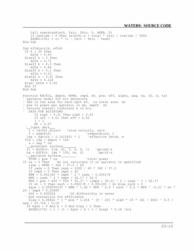
WATER9: SOURCE CODE
23-19
Call sumrates8(nt%, fair, fbio, 0, AREA, 0)If restime > 0 Then le(nt%).e = total * fair / restime / 3600ASGN2(192) = ci * (1 - fair - fbio - fads)
End Sub
Sub k25dcorr(k, m25d)If k > 30 Then
m25d = 0.93ElseIf k > 3 Then
m25d = 0.75ElseIf k > 0.5 Then
m25d = 0.44ElseIf k > 0.1 Then
m25d = 0.15ElseIf k > 0.01 Then
m25d = 0.124Else: m25d = 0.02End If
End Sub
Function KAC8(L, depth, RPMS, impd, dv, pow, eff, alpha, aag, na, dl, k, ta)' agitator model for air emissions' AAG is the area for each agit m2, ta total area m2' pow is power per agitator in hp, depth cm' returns overall turbulent k in m/s' DATA FOR AGITATORS
If alph < 0.01 Then alph = 0.83If eff < 0.01 Then eff = 0.83j = 3EP = 0.67
'__input data___v = ld(50).dissol 'wind velocity, cm/sT = asgn8(2) 'temperature, C
ldw = Sqr(ta / 3.141592) * 2 'effective fetch, mfld = ldw / depth * 100
a = aag * na'__quiescent surface_______kl = KLC8(v, fld, dl, T, 6, 0, 1) 'gm/cm2-skg = KGC8(v, ldw * 100, dv, 2) 'gm/c2-s
'__agitated surface________TPOW = pow * na 'total power
If na > 0 Then 'do not calculate if no agitator is specifiedrads = RPMS * 360 / 57.3 / 60If rads = 0 Then rads = 1200 / 60 * 360 / 57.3If impd = 0 Then impd = 60NRW = 0.001185 * impd ^ 2 * rads / 0.000178NFR = rads ^ 2 * impd / 32.17 / 30.5NPR = pow * eff * 550 * 32.17 / (impd / 30.5) ^ 5 / rads ^ 3 / 62.37If dv > 0 Then nsch = 0.000178 / 0.001185 / dv Else nsch = 0kgre = 0.000000135 * NRW ^ 1.42 * NPR ^ 0.4 * nsch ^ 0.5 * NFR ^ -0.21 * dv *
29 / impd * 0.00409DO2 = 0.000024 'O2 diffusivity in water
' pow correction for efficiencyklag = 0.00822 * j * pow * 1.024 ^ (T - 20) * alph * 18 * (dl / DO2) ^ 0.5 /
aag / 10.764 / 0.18If kgre > 0 And k > 0 And klag > 0 ThenASGN2(174) = 1 / (1 / kgre / k + 1 / klag) * 0.18 'm/s
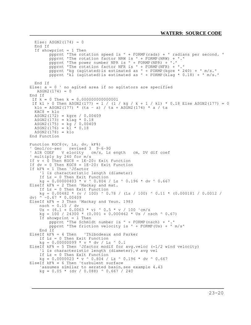
WATER9: SOURCE CODE
23-20
Else: ASGN2(174) = 0End IfIf showprint = 1 Then
ppprnt "The rotation speed is " + FORMP(rads) + " radians per second. "ppprnt "The rotation factor NRW is " + FORMP(NRW) + "."ppprnt "The power number NPR is " + FORMP(NPR) + "."ppprnt "The rotation factor NFR is " + FORMP(NFR) + "."ppprnt "kg (agitated)is estimated as " + FORMP(kgre * 240) + " m/s."ppprnt "kl (agitated)is estimated as " + FORMP(klag * 0.18) + " m/s."
End IfElse: a = 0 ' no agited area if no agitators are specified
ASGN2(174) = 0End IfIf k = 0 Then k = 0.000000000000001If kl > 0 Then ASGN2(177) = 1 / (1 / kg / k + 1 / kl) * 0.18 Else ASGN2(177) = 0klo = ASGN2(177) * (ta - a) / ta + ASGN2(174) * a / taKAC8 = kloASGN2(172) = kgre / 0.00409ASGN2(173) = klag * 0.18ASGN2(175) = kg / 0.00409ASGN2(176) = kl * 0.18ASGN2(178) = klo
End Function
Function KGC8(v, Lz, dv, kF%)' Gmol/cc-sec revised 3 9-6-90' AIR COEF V elocity cm/s, Lz ength cm, DV dif coef' multiply by 240 for m/sIf v < 0 Then KGC8 = 1E-20: Exit FunctionIf dv = 0 Then KGC8 = 1E-20: Exit FunctionIf kF% = 1 Then 'Jfactor
'l is characteristic length (diameter)If Lz = 0 Then Exit Functionkg = 0.00000403 * v ^ 0.804 / Lz ^ 0.196 * dv ^ 0.667
ElseIf kF% = 2 Then 'Mackay and mat.If Lz = 0 Then Exit Functionkg = 0.00482 * (v / 100) ^ 0.78 / (Lz / 100) ^ 0.11 * (0.000181 / 0.0012 /
dv) ^ -0.67 * 0.00409ElseIf kF% = 3 Then 'Mackay and Yeun. 1983
nsch = 0.15 / dvUs = (6.1 + 0.0063 * v) ^ 0.5 * v / 100 'cm/skg = 100 / 24300 * (0.001 + 0.000462 * Us / nsch ^ 0.67)If showprint = 1 Then
ppprnt "The Schmidt number is " + FORMP(nsch) + "."ppprnt "The friction velocity is " + FORMP(Us) + " m/s"
End IfElseIf kF% = 4 Then 'Thibodeaux and Parker
If Lz = 0 Then Exit Functionkg = 0.00000099 * v * dv / Lz ^ 0.1
ElseIf kF% = 5 Then 'Jfactor modif for avg.veloc (=1/2 wind velocity)'l is characteristic length (diameter),v avg velIf Lz = 0 Then Exit Functionkg = 0.0000023 * v ^ 0.804 / Lz ^ 0.196 * dv ^ 0.667
ElseIf kF% = 6 Then 'turbulent surface'assumes similar to aerated basin,see example 4.43kg = 0.05 * (dv / 0.088) ^ 0.667 / 240

WATER9: SOURCE CODE
23-21
End IfIf kg = 0 Then kg = 0.001 * 100 / 24300 'default, 4.1e-6If showprint = 1 Then
ppprnt "kg is estimated as " + FORMP(kg * 240) + " m/s."End If
KGC8 = kg
End Function
Sub Kgp8(pd, pa, G, kg)'calculates the gas phase mass transfer coef for a packed bed.'used for trickling filters : important for low Henry's law compounds'Kg cm/s ; G gmol/s-cm2If G = 0 Then kg = 0: Exit SubScg = 0.00018 / 0.0011 / 0.088 '%% aa.dvkg = G * Scg ^ -0.666 * 1.1958 * (pd * G * 29 / 0.00018 / (1 - pa)) ^ -0.36kg = kg * 24000End Sub
Function KLC8(v, Hl, dl, T, fx%, slope, rough)' WIND EQUATIONS FOR LIQUID COEF (G-M/CM2/SEC)' V elocity wind cm/s DL dif coef cm2/s' T emperature C HL depth cm' slope rise/run rough cm, 7=fraction flow' __specifications
DBL = 0.00001DOW = 0.000025EP = 0.7If dl = 0 Or v < 0 Or Hl <= 0 Then KLC = 1E-20: Exit Functionnsch = 0.01 / dl 'Schmidt numberUs = (6.1 + 0.0063 * v) ^ 0.5 * v / 100 'friction velocity cm/sIf fx% = 1 Then
REF = 48 * v ^ 1.25 / (Exp(56.6 / v ^ 0.25))kl = (17.6 * REF ^ 0.195 - 7.72) * 0.00001 * (dl / DBL) ^ EP
ElseIf fx% = 2 Then 'owens edwardskl = 3.314 * (1.024 ^ (T - 20)) * v ^ 0.67 / ((Hl / 3) ^ 0.85) * DOW * (dl /
DOW) ^ EPElseIf fx% = 3 Then 'owens,et.all 1964 (trench model)
'v=water velocity cm/skl = 0.000783 * (v) ^ 0.67 / (Hl) ^ 0.85 * (dl / DOW) ^ EP
ElseIf fx% = 4 Then 'churchillkl = 0.00078 * (v) ^ 0.69 / (Hl) ^ 0.853 * (dl / DOW) ^ EP
ElseIf fx% = 5 Then 'Mackay and Yeun (1983)If Us > 30 Thenkl = (0.000001 + 0.0000341 * Us * nsch ^ (-0.5)) * 100 / 18
Elsekl = (0.000001 + 0.0144 * (Us / 100) ^ 2.2 * nsch ^ (-0.5)) * 100 / 18
End IfElseIf fx% = 6 Then 'springerfd = Hl 'F/D IS EQUAL TO HL IN CASE 6If v < 325 Then 'cm/s
If showprint = 1 Then ppprnt "The velocity is " + FORMP(v) + " cm/s."kl = 0.00000278 * (dl / 0.0000085) ^ 0.66666
ElseIf fd > 51.11 ThenIf showprint = 1 Then ppprnt "The fetch to depth ratio is " + FORMP(fd) +
"."
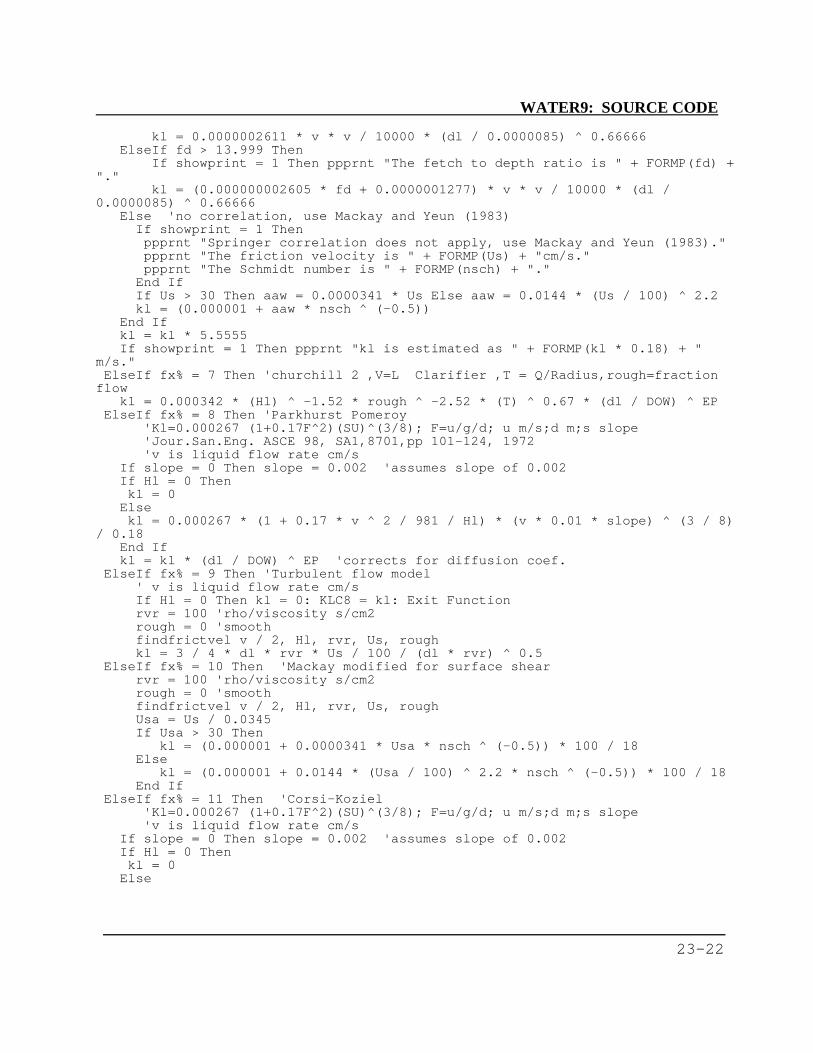
WATER9: SOURCE CODE
23-22
kl = 0.0000002611 * v * v / 10000 * (dl / 0.0000085) ^ 0.66666ElseIf fd > 13.999 Then
If showprint = 1 Then ppprnt "The fetch to depth ratio is " + FORMP(fd) +"."
kl = (0.000000002605 * fd + 0.0000001277) * v * v / 10000 * (dl /0.0000085) ^ 0.66666
Else 'no correlation, use Mackay and Yeun (1983)If showprint = 1 Thenppprnt "Springer correlation does not apply, use Mackay and Yeun (1983)."ppprnt "The friction velocity is " + FORMP(Us) + "cm/s."ppprnt "The Schmidt number is " + FORMP(nsch) + "."
End IfIf Us > 30 Then aaw = 0.0000341 * Us Else aaw = 0.0144 * (Us / 100) ^ 2.2kl = (0.000001 + aaw * nsch ^ (-0.5))
End Ifkl = kl * 5.5555If showprint = 1 Then ppprnt "kl is estimated as " + FORMP(kl * 0.18) + "
m/s."ElseIf fx% = 7 Then 'churchill 2 ,V=L Clarifier ,T = Q/Radius,rough=fraction
flowkl = 0.000342 * (Hl) ^ -1.52 * rough ^ -2.52 * (T) ^ 0.67 * (dl / DOW) ^ EP
ElseIf fx% = 8 Then 'Parkhurst Pomeroy'Kl=0.000267 (1+0.17F^2)(SU)^(3/8); F=u/g/d; u m/s;d m;s slope'Jour.San.Eng. ASCE 98, SA1,8701,pp 101-124, 1972'v is liquid flow rate cm/s
If slope = 0 Then slope = 0.002 'assumes slope of 0.002If Hl = 0 Thenkl = 0
Elsekl = 0.000267 * (1 + 0.17 * v ^ 2 / 981 / Hl) * (v * 0.01 * slope) ^ (3 / 8)
/ 0.18End Ifkl = kl * (dl / DOW) ^ EP 'corrects for diffusion coef.
ElseIf fx% = 9 Then 'Turbulent flow model' v is liquid flow rate cm/sIf Hl = 0 Then kl = 0: KLC8 = kl: Exit Functionrvr = 100 'rho/viscosity s/cm2rough = 0 'smoothfindfrictvel v / 2, Hl, rvr, Us, roughkl = 3 / 4 * dl * rvr * Us / 100 / (dl * rvr) ^ 0.5
ElseIf fx% = 10 Then 'Mackay modified for surface shearrvr = 100 'rho/viscosity s/cm2rough = 0 'smoothfindfrictvel v / 2, Hl, rvr, Us, roughUsa = Us / 0.0345If Usa > 30 Then
kl = (0.000001 + 0.0000341 * Usa * nsch ^ (-0.5)) * 100 / 18Else
kl = (0.000001 + 0.0144 * (Usa / 100) ^ 2.2 * nsch ^ (-0.5)) * 100 / 18End If
ElseIf fx% = 11 Then 'Corsi-Koziel'Kl=0.000267 (1+0.17F^2)(SU)^(3/8); F=u/g/d; u m/s;d m;s slope'v is liquid flow rate cm/s
If slope = 0 Then slope = 0.002 'assumes slope of 0.002If Hl = 0 Thenkl = 0
Else
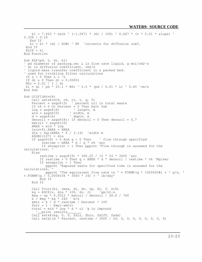
WATER9: SOURCE CODE
23-23
kl = 7.603 * nsch ^ (-1.047) * (Hl / 100) ^ 0.667 * (v * 0.01 * slope) ^0.338 / 0.18
End Ifkl = kl * (dl / DOW) ^ EP 'corrects for diffusion coef.
End IfKLC8 = kl
End Function
Sub KLP(pd, L, dl, kl)' pd diameter of packing,cm; L is flow rate liquid, g mol/cm2-s' dl is diffusion coefficient, cm2/s' liquid mass transfer coefficient in a packed bed.' used for trickling filter calculationsIf L < 0 Then L = -LIf dl = 0 Then dl = 0.00001NSc = 0.01 / 1 / dlkl = dl / pd * 25.1 * NSc ^ 0.5 * (pd / 0.01 * L) ^ 0.45 'cm/s
End Sub
Sub OILFILM(nt%)Call sets8(nt%, n%, ci, v, q, T)Percent = asgn8(3) ' percent oil in total wasteIf n% = 0 Or Percent = 0 Then Exit SubLng = asgn8(4) ' length, mwid = asgn8(5) ' width, md = asgn8(6) ' depth, mdensoil = asgn8(8): If densoil = 0 Then densoil = 0.7mwtoil = asgn8(10)AREA = wid * Lngle(nt%).AREA = AREAdia = Sqr(AREA * 4 / 3.14) 'width mASGN2(107) = diaIf asgn8(9) = 0 And q > 0 Then ' flow through specified
restime = AREA * d / q * n% 'secIf showprint = 1 Then ppprnt "Flow through is assumed for the
calculations. "Else
restime = asgn8(9) * 365.25 / 12 * 24 * 3600 'secIf restime > 0 Then q = AREA * d * densoil / restime * n% 'Mg/secIf showprint = 1 Then
ppprnt "Exposed waste for specified time is assumed for thecalculations. "
ppprnt "The equivalent flow rate is " + FORMP(q * 1000000#) + " g/s, "+ FORMP(q / 0.0004536 * 3600 * 24) + " lb/day"
End IfEnd If
Call Tcorr(k1, vmax, dl, dv, vp, Hl, T, nt%)kg = KGC8(v, dia * 100, dv, 2) 'gm/c2-sKeq = vp * 0.0012 * mwtoil / densoil / 28.8 / 760k = Keq * kg * 240 ' m/sxmtr = k / d * restime / Percent * 100fair = 1 - Exp(-xmtr)total = wid * Lng * d * ci 'g in impound
'__print results_______Call setx8(kg, 0, 0, fair, fbio, fdiff, fads)Call setx1(d * Percent, restime / 3600 / 24, 0, 0, 0, 0, 0, 0, 0, 0)

WATER9: SOURCE CODE
23-24
If restime > 0 Then le(nt%).cin = total / restime 'g/sCall sumrates8(nt%, fair, 0, 0, ta, 0)If restime > 0 Then le(nt%).e = total * fair / restimeASGN2(192) = ci * (1 - fair - fbio - fads)If showprint = 1 Then
ppprnt "The model assumes gas phase resistance only. " + FORMP(kg) +"gm/c2-s"
ppprnt "The initial loss is " + FORMP(k / d / Percent * 100 * total) + "g/s"
ppprnt "The model assumes first order decay during residence for emissionloss."
End If
End Sub
Sub PRETREATMENT(nt%)'unit% 1 bar screen 2 grit chamber 3 open trenchCall sets8(nt%, n%, ci, v, q, T)rough = 0.007 * 2.54 * 12 ' sewer wall roughness, ft to (cm)If n% = 0 Or q = 0 Then e = 0: fair = 0: Exit Sub 'unit not present'__input parameters__Length = asgn8(4) ' length, mAREA = asgn8(5) * Length * n% 'm2le(nt%).AREA = AREAASGN2(107) = Sqr(AREA * 4 / 3.14) 'width md = asgn8(6) 'mair = asgn8(7) 'm3/s air per unit
' If L(nt%).wflow > 0 Then oilfract = L(nt%).oil / L(nt%).wflow / 1000oilsurf = asgn8(9) 'fraction of surface covered with oilmwtoil = asgn8(10)densoil = asgn8(11): If densoil = 0 Then densoil = 0.7ventrate = asgn8(16) * asgn8(4) * asgn8(5) 'm3/s per m2 area * m2 areacover% = asgn8(17)MUNICIPAL% = asgn8(14)controlf = asgn8(15)If ld(50).waste2 = 2 Then 'WATER8 compatability mode
oilfract = asgn8(8) / 100Call fractionoil(oilfract, owpc, owr, frinoil, 0)
ElseCall fractionoil(oilfract, owpc, owr, frinoil, n%)
End Ifrtime = AREA * d / q 's
'__calculate mass transfer coef.__vl = Length * 100 / rtime 'cm/sCall Tcorr(k1, vmax, dl, dv, vp, Hl, T, nt%)kg = KGC8(v, Length * 100, dv, 3)updateventin nt%, 0, ci, q, AREA * d, air, vair
If trenchunit = 1 Then 'trenchIf MUNICIPAL% = 1 Then'---Parkhurst and Pomeroy, 1972 g-m/cm2-skl = KLC8(vl, d * 100, dl, T, 8, 0, rough)
Elsekl = KLC8(vl, d * 100, dl, T, 3, 0, rough)
End If

WATER9: SOURCE CODE
23-25
Elsekl = asgn8(3) / 0.18 '__specified value
End IfIf kl = 0 Then kl = 1E-20: kg = 1E-20 'covered surfaceHcorr = Hl * (1 - frinoil)If Val(Hcorr) < 0.000000000000001 Then Hcorr = 0.00000000000001If showprint = 1 Then ppprnt "The oil corrected HL is " + Format$(Hl * (1 -
frinoil) * 55555, "#.###e+00 (y/x)")
'_____water surfaceko = 1 / (1 / kl + 1 / Hcorr / 55555 / kg) * 0.18 'm/sMtr = ko * AREA * (1 - oilsurf) / q
'_____oil surfaceKeq = vp * 0.0012 * mwtoil / densoil / 28.8 / 760k = Keq * kg * 240 ' m/smtr3 = k * AREA * oilsurf * owpc / q
'_____air bubblesairdens = 1 / 0.0224 * 273 / (273 + T) 'g-m/m3mtr2 = air * n% * Hcorr * airdens / q
'_____vent under coverMtrvent = ventrate * n% * Hcorr * airdens / q
'_____summationIf cover% = 1 Then
'Mtr = 0: mtr3 = 0If Mtr = 0 Then Mtr = 1E-20fair2 = 1 - Exp(-mtr2) ' air bubblesfair3 = 0fairmaxVent = 1 - Exp(-Mtrvent) 'equilib vent under coverfairmaxMtr = 1 - Exp(-(Mtr + mtr3)) 'mass transfer oil and waterIf fairmaxVent > fairmaxMtr Then ftot = fairmaxMtr Else ftot = fairmaxVentfair1 = (1 - fair2) * ftot * Mtr / (Mtr + mtr3)fair3 = (1 - fair2) * ftot * mtr3 / (Mtr + mtr3)fair = fair2 + fair1 + fair3
Elsecontrolf = 0sumMtr = (Mtr + mtr2 + mtr3)fair = 1 - Exp(-sumMtr)fair1 = fair * Mtr / sumMtrfair2 = fair * mtr2 / sumMtrfair3 = fair * mtr3 / sumMtr
End If
'___print results
Call setx1(Hcorr * 55555, frinoil, fair3, 0, 0, 0, 0, 0, fair1, fair2)Call setx8(kg, kl, ko / 0.18, fair, fbio, fdiff, fads)Call sumrates8(nt%, fair, fbio, fads, AREA, controlf)
endptreat:End Sub
Sub SEPARATOR(nt%)'calculates separator'_______ input variables___________
Call sets8(nt%, n%, ci, windvelocity, q, T)Call Tcorr(k1, vmax, dl, dv, vp, Hl, T, nt%)airdens = 1 / 0.0224 * 273 / (273 + T) ' g-m/m3ta = asgn8(3) / 10000 'Total gas exit area m2
WATER9: SOURCE CODE
23-26
G = asgn8(4) * 0.00508 'gas velocity (m/s)oilfract = asgn8(12) / 100 'fract oilremoval = asgn8(11) 'fraction oil recovery in unitheadspace1 = asgn8(9)Lm = q * 1000000 / 18 / n% 'moles/s liquidIf q = 0 Then Exit SubCall fractionoil(oilfract, owpc, owr, frinoil, 0)koc = (Hl * (1 - frinoil) * 55555)
'--mass transferventperarea = asgn8(8) 'm2widths = asgn8(6)Length = asgn8(5)depth = asgn8(7)areasurface = Length * widths 'm2le(nt%).AREA = areasurface
'If areasurface = 0 Then areasurface = 1 'minimumIf G > 0 Thenair = G * ta 'emitted air m3/s
ElseIf areasurface > 0 Thenair = ventperarea * areasurface
Elseair = ventperarea * 0.1 'minimum amount of air flow
End Ifgm = airdens * air 'moles/s gas
'____equilibrium________frapart = air * Hl * (1 - frinoil) * airdens / q * n%faire = air * Hl * (1 - frinoil) * airdens / (q / n% + air * Hl * (1 -
frinoil) * airdens)fair = faire 'assumes equilibrium with exit'-------restime = areasurface * depth / q * n% 'sIf restime = 0 Then
frequil = 1Else
vcl = Length / restime * 100 'water vel, cm/sIf widths * headspace1 = 0 Then
v = 10 'cm/sElse
v = air / (headspace1 * widths) * 10000 'cm/sEnd Ifskg = KGC8(v, headspace1, dv, 3) 'gm/c2-sskl = KLC8(vcl, depth * 100, dl, T, 4, 0, 1) 'gm/c2-sIf skl < 1E-20 Then skl = 1E-20sko = 1 / (1 / skl + 1 / (Hl * (1 - fadso)) / 55555 / skg) 'gm/c2-sMtr = sko * 0.18 / depth * restimesfair = 1 - Exp(-Mtr)
sko = 0.001 'm/skoc = (Hl * (1 - frinoil) * 55555)arear = areasurface 'area m2kor = sko * 0.18 'm/s

WATER9: SOURCE CODE
23-27
Lm = q * 1000000 / 18 / n% 'moles/s liquidghx = gm * kocskor = arear / q * n% * kor * (1 + Lm / ghx) 'm3/s per m3/sfair = 1 - (ghx / (Lm + ghx) * Exp(-skor) + Lm / (Lm + ghx))If Lm / ghx > 1E+20 Then
frequil = fair * Lm / ghxElse
frequil = fair / (1 - Lm / (Lm + ghx))End If
End If'-------oilrecovery = removal * oilfract * q / n%If oilfract > 0 Then oilconc = frinoil * ci / oilfract Else oilconc = 0fads = removal * frinoil * (1 - fair)airconcg = ci * q / n% * fair / air 'g/m3If aa.mwt = 0 Then aa.mwt = 100airconc = airconcg / aa.mwt / airdens * 1000000
'____print the results______Call setx1(T, 0, air, airconc, koc, frinoil, oilrecovery, oilconc, fads, fair)ASGN2(182) = frequilASGN2(183) = skg / 0.00409ASGN2(184) = skl * 0.18ASGN2(185) = sko * 0.18
Call sumrates8(nt%, fair, 0, fads, ta, 0)End Sub
Sub SetSteamK()'finds K for steam stripper conditionspsiA! = asgn8(9)sx$ = " .088.178 .51 1.27 2.22 4.74 11.5 14.7 20.8"sy$ = " 0 10 27 43 54 71 93 100 110"setvar 5, psiA!, tcolumn!, sx$, sy$asgn8(3) = tcolumn! - 5 ' inlet feed 5 c lessHenryLaw tcolumn!, aa.n, steamstripK, hIf tcolumn! < 105 And tcolumn! > 95 Then steamstripK = aa.ksspH = asgn8(19)ionization steamstripK, pHasgn8(13) = steamstripK
End Sub
Sub SteamLGcalc(gl!, lg!, n!, texit, lout!, gout!)Ttop = asgn8(3)Tfeedin = asgn8(8)concin = asgn8(12)gl! = asgn8(4) 'steam rate (mol gas/ mol liquid)n! = asgn8(6)psig! = asgn8(7)psiA! = asgn8(9)If gl! = 0 Then gl! = 0.1lg! = 1 / gl!l1! = 1 'assume 1 g/s feedG! = gl! * l1!lout! = l1!
WATER9: SOURCE CODE
23-28
cpl! = 1#delhfeed! = (Ttop - Tfeedin) * l1! * cpl! 'cal/s to preheater
'STEAM PROPERTIESsx$ = " 0 1.69 27.1 42.9 63 103 159 232 1000"sy$ = " 1150 1160 1171 1176 1183 1190 1196 1201 1206"setvar 5, psig!, delhsteamin!, sx$, sy$'PRESSURE PROPERTIESsx$ = " .088.178 .51 1.27 2.22 4.74 11.5 14.7 20.8"sy$ = " 0 10 27 43 54 71 93 100 110"setvar 5, psiA!, coltemp!, sx$, sy$asgn8(14) = coltemp!'frmStripper!label25.Caption = Str$(coltemp!)'PRESSURE PROPERTIESsx$ = " .088.178 .51 1.27 2.22 4.74 11.5 14.7 20.8"sy$ = " 1076 1084 1097 1090 1118 1130 1145 1150 1157"setvar 5, psiA!, ColBTU!, sx$, sy$
delhfeed1! = (coltemp! - Ttop) * 1.8 'Btu/lb heater to tray' delhsteam! = (delhsteamin! - 1150) * g!'Btu/lb steam add heat
delhsteam! = (delhsteamin! - ColBTU!) * G! 'Btu/lb steam add heatdelhvap! = (ColBTU! - 180.07 + (100 - coltemp!) * 1.8) 'BTU/g steam to liqgcol! = G! + delhsteam! / delhvap!gout! = gcol! - delhfeed1! / delhvap!lcol! = l1! + delhfeed1! / delhvap!lout! = lcol! - delhsteam! / delhvap!lg! = lcol! / gcol!texit = coltemp! - delhfeed! / lout! / cpl!
End SubPublic Sub stripper(G, Lm, k, bio, kl, n, rt, YI, Yo, xi, Xo, fair, fbio, cmtr)On Error GoTo errorstrippers' countercurrent gas-liquid flow with mass transfer and first-order reaction'(G, l, k, b, kL, n, rt, yi, yo, xi, xo, fair, fbio)' rewritten 8-6-99 yin can be different from 0' backcalc from gas side' check for overcalc' Rt residence time in system sec' N number of calculation elements' Kl mass trans. /s' Bio biorate constant /s' G L moles/s' k partition coefficient (y/x)'fair <0 then refers to gas phase' cmtr g/s transferred to liquid valid if bio=0''_____clean up incorrect inputsIf YI < 0 Then YI = 0fair = 0cmtr = 0If xi < 0 Then xi = 0If Lm <= 0 Or G = 0 Then Yo = YI: Xo = xi: Exit Sub
maxmtr = (YI - xi * k) * G 'molsmaxyo = ki * k: If maxyo < YI Then maxyo = YIIf maxmtr > 0 Then maxxo = xi + maxmtr / Lm Else maxxo = xi

WATER9: SOURCE CODE
23-29
If k < 1E-20 Then k = 1E-20n = Int(n)If n > 99 Then n = 99 'limit to 100dt = rt / n '__ estimate time step for each increment
EE = Lm / GEf = EE + EE * bio * dtc1 = 1 / (kl * dt + 1 + dt * bio)c2 = dt * kl * c1 / kDim aa1(100), aa2(100), bb1(100), bb2(100)
aa1(0) = xiaa2(0) = 0aa1(1) = xi * c1aa2(1) = c2bb1(1) = 0bb2(1) = 1'y(i)=bb1(i)+bb2(i)*yo'x(i)=aa1(i)+aa2(i)*yobiosuma = 0biosumb = 0For i = 1 To n
bb1(i + 1) = Ef * aa1(i) - EE * aa1(i - 1) + bb1(i)bb2(i + 1) = Ef * aa2(i) - EE * aa2(i - 1) + bb2(i)aa1(i + 1) = c1 * aa1(i) + c2 * bb1(i + 1)aa2(i + 1) = c1 * aa2(i) + c2 * bb2(i + 1)biosuma = biosuma + aa1(i)biosumb = biosumb + aa2(i)
NextYo = (YI - bb1(n + 1)) / bb2(n + 1)biosum = dt * bio * (biosuma + biosumb * Yo)Xo = aa1(n) + aa2(n) * Yocheckerrors:totali = YI * G + xi * Lmtotalo = Yo * G + Xo * LmIf totali > 0 Then fbio = Lm * biosum / totali Else fbio = 0 'mol/s bio per mol/stransratio = kl * Lm / G / kIf Xo < 1E-20 Then Xo = 1E-20'__check for errors in calculations__error2 = 0If Xo > maxxo ThenXo = maxxo: error2 = 1
End Ifyotest = (xi * Lm + YI * G - Xo * Lm) / GIf yotest <= maxyo And bio = 0 Then 'base yo on xo
Yo = yotestElseIf error2 = 1 Then 'base xo on yo
Yo = maxyoXo = (xi * Lm + YI * G - Yo * G) / Lm
End IfIf Yo < 0 Then Yo = 0If Xo < 0 Then Xo = 0If YI > Yo Then
cmtr = aa.mwt * ((YI - Yo) * G) 'g/s %%%%

WATER9: SOURCE CODE
23-30
fair = 0ElseIf xi > Xo Then
fair = (xi - Xo) / xiElse
fair = 0End IfBreak = Break
Exit Sub'_____________________
errorstrippers:'equilibrium one stage if defective moduletotali = YI * G + xi * LmIf totali <= 0 Then totali = 0If xi < 0 Then xi = 0Xo = totali / (Lm + k * G)Yo = Xo * k
Resume checkerrors
End Sub
Sub stripper8(G, L, k, b, kl, n, rt, YI, Yo, xi, Xo, fair, fbio)'used for trickling filter model' b = 0'(G, l, k, b, kL, n, rt, yi, yo, xi, xo, fair, fbio)' rewritten 9-17-93 assumes yin =0' Rt residence time sec' N number of calculation elements' Kl mass trans. /s' B biorate constant /s' G L moles/s' initial concentration in air=0' k partition coefficient (y/x)If k < 1E-20 Then k = 1E-20n = Int(n)dt = rt / n '__ estimate time step for each incrementa = 1 + b * dt + kl * dtb2 = -kl / k * dtc = k * G / (k * G + kl * L * dt)d = c * kl * L / G * dt'YI = 0 if by definitionxxl = 1: yg = YI 'initialize the valuesFor i = 1 To n
yg = c * yg + d * xxlxxl = a * xxl + b2 * yg
NextXo = xi / xxlYo = yg * xi / xxltotal = xi * L + YI * GIf total = 0 Then total = 1fair = (Yo - YI) * G / totalfbio = ((xi - Xo) * L - (Yo - YI) * G) / total'__check for errors in calculations__'If fair > 1! Then fair = 1
WATER9: SOURCE CODE
23-31
'If fair < 0 Then fair = 0If fbio < 0.00001 Then fbio = 0If L = 0 Then Yo = YIEnd Sub
Sub TANK(nt%)'$DYNAMIC' 5-3-94Call sets8(nt%, n%, ci, Vel, q, temp)
dt = asgn8(10) * 1.8 'deg FFp = asgn8(7) 'paint factor
storetime = asgn8(6) 'dayswid = asgn8(8) 'diameter m
h = asgn8(9) 'vapor space mAREA = (wid) ^ 2 * 3.141592 / 4 'm2le(nt%).AREA = AREA
depth = asgn8(11) 'm specified as tank heightDENS = asgn8(4) 'g/ccmwt = asgn8(5)vol = depth * AREA ' m3
areareal = asgn8(3)oilfract = asgn8(12) / 100If oilfract = 0 Then 'oil fraction not specified, estimated from inflow
Call fractionoil(oilfract, owpc, owr, frinoil, nt%)Else
Call fractionoil(oilfract, owpc, owr, frinoil, 0)End Iffair = 0: fairs = 0: fairb = 0: fairw = 0
If storetime = 0 And q = 0 ThenExit Sub
ElseIf storetime = 0 Thenstoretime = vol * n% / q / 3600 / 24
End IfIf storetime = 0 Then Exit Subqan = n% * ci * vol * DENS / storetime * 365 'g yearly throughputnturn = 365 / storetime
Call Tcorr(k1, vmax, dl, dv, vp, Hl, temp, nt%)cmwt = aa.mwt: If cmwt = 0 Then cmwt = 80If nturn <= 36 Then Kn = 1 Else Kn = (180 + nturn) / 6 / nturnIf mwt = 18 Or oilfract = 0 Then 'aqueous
p = 14.7 * Hl * ci / cmwt * (1 - frinoil) 'psiapmax = vp / 760 * 14.7If p > pmax Then p = pmaxaqueous$ = " Aqueous matrix"If showprint = 1 Then ppprnt "The oil corrected aqueous HL is " +
Format$(Hl * (1 - frinoil) * 55555, "#.###e+00 (y/x)")xw = 0
Elsecoil = ci * frinoil / oilfractxw = frinoil * coil / cmwt / (coil / cmwt + (1000000! - coil) / mwt)p = xw * vp * 14.7 / 760 'psiaaqueous$ = " Oily matrix"
End IfIf p < 0 Then p = 0

WATER9: SOURCE CODE
23-32
conc = p / 14.7 / 1000000! 'ppmvIf showprint = 1 Then
ppprnt "The concentration in the tank inlet is " + Format$(ci,"#.###e+00 ppmw")
ppprnt "The flowrate of liquid is " + Format$(q, "#.###e+00") + "M3/s"
ppprnt "liquid flowrate (from tank holding) is " + Format$(vol /storetime / 24 / 3600, "#.###e+00") + " M3/s"
ppprnt "The total loading of the compound is " + Format$(qan,"#.##e+00") + " g/yr."
End IfIf areareal > 0 Then
If depth = 0 Then depth = 0.3fd = wid / depthkg = KGC8(Vel, wid * 100, dv, 2)kl = KLC8(Vel, fd, dl, temp, 6, 0, 1)ko = 1 / (1 / kl + 1 / Hl / 55555 / kg)restime = storetime * 24 * 3600Mtr = ko * 0.18 / depth * restimefairs = 1 - Exp(-Mtr)fair = fairsCall setx8(kg, kl, ko, fairs, 0, 0, 0)
Else'_____working losses
If depth = 0 Then 'assumes constant level tank, fixed rooffairw = 0
ElseG = q * 1000 / 3.75 * 3600 * 24 'gal/dayv = vol * 1000 / 3.785 'gallw = 0.0000000109 * aa.mwt * p * v * Kn 'Mg/turnoverIf ci > 0 Then fairw = 1000000! * lw / (ci * vol * DENS) Else fairw = 0fairw = fairw / (1 + fairw)If showprint = 1 Then
ppprnt "The working volume is " + Format$(vol, "#.###e+00 m3;") +Format$(v, "#.###e+00 gal")
ppprnt "The mass lost per turnover is " + Format$(lw, "#.###e+00") +" Mg/turnover"
ppprnt "The vapor pressure of the compound in solution is " +Format$(p, "#.######") + " atm."
End IfEnd If
'_____breathing lossesdia = wid * 3.28 'fth = h * 3.28 'ftIf dia > 30 Then c = 1 Else c = 0.0771 * dia - 0.0013 * dia ^ 2 - 0.1334Lb2 = 0.0000102 * aa.mwt * (p / (14.7 - p)) ^ 0.68 * dia ^ 1.73Lb = n% * Lb2 * h ^ 0.51 * dt ^ 0.5 * Fp * c 'Mg/yearIf qan > 0 Then fairb = 1000000 * Lb / qan Else fairb = 0fairb = fairb / (1 + fairb)fair = fairb + fairw * (1 - fairb)Call setx8(0, 0, 0, 0, 0, 0, 0)If showprint = 1 Then
ppprnt "MWT = " + Format$(aa.mwt, "###.#") + " dia= " +Format$(dia, "####.# ft.")
ppprnt "Breathing: Lb = 0.0000102 * MWT * (p / (14.7 - p)) ^ 0.68 *dia ^ 1.73 "
ppprnt "mass emissions= Lb * h ^ 0.51 * dt ^ 0.5 * Fp * c Mg/yr"

WATER9: SOURCE CODE
23-33
ppprnt "c = " + Format$(c, "#.###") + " h= " + Format$(h, "####.#ft.")
ppprnt "dt = " + Format$(dt, "##.## ") + "deg.F Fp= " +Format$(Fp, "##.###")
ppprnt "mass emissions= " + Format$(Lb, "##.##E+00 ") + " Mg/yr"End If
End If
If showprint = 1 Thenppprnt "The temperature in the tank is " + Format$(temp, "###.#") + " deg.C"ppprnt "The type of liquid is " + aqueous$ppprnt "The concentration in the liquid waste is " + Format$(ci, "#.###e+00
g/m3")ppprnt "The fraction in the oil is " + Format$(frinoil, "#.#######")ppprnt "The vapor pressure (p) is " + Format$(p, "#.###e+00 psia; ") + "(" +
Format$(vp, "#.###e+00 mmHg") + ")"ppprnt "The fraction of the compound in oil phase is " + Format$(frinoil,
"#.#####") + "."ppprnt "The residence time in the tank is " + Format$(storetime, "###.###") + "
days."End If
Call setx1(storetime, Kn, fairw, fairb, fairs, concg, frinoil, 0, 0, 0)Call sumrates8(nt%, fair, 0, 0, AREA, 0)ASGN2(192) = ci * (1 - fair - fbio - fads)
End Sub
Sub Tcorr(xk1, vmax, dl, dv, vp, Hl, T, nt%)If showprint = 1 Then
ppprnt "Properties of " + bTrim$(aa.cs) + " at " + Format$(T, "###.#") +" deg.C"
End Ifvmax = aa.biov * (1.046 ^ (T - 25))d = ((T + 273.16) / 298.16)dv = aa.dv * d ^ 1.75 'cm2/sdl = aa.dl * d 'cm2/sIf aa.c + T = 0 Then c = 0 Else c = Exp(-aa.b * 2.30258 * (1 / (aa.c + T) - 1
/ (aa.c + 25)))HL1 = aa.HlIf nt% < 0 Then
pH = -nt%ElseIf nt% > 0 Then
pH = L(nt%).pHEnd IfIf pH <> 0 And HL1 > 0 Then
If Mid$(aa.code, 6, 1) = "k" Or Mid$(aa.code, 6, 1) = "b" ThenKa = aa.rhIf pH = 0 Or Ka = 0 ThenElseoH3 = 10 ^ (-pH)comp2 = Ka / oH3If Mid$(aa.code, 6, 1) = "k" Then
HL1 = HL1 / (1 + comp2)ElseIf Mid$(aa.code, 6, 1) = "b" Then
HL1 = HL1 * comp2 / (1 + comp2)End If

WATER9: SOURCE CODE
23-34
If showprint = 1 Thenppprnt " pH = " + FORMP(pH)ppprnt " Ka = " + FORMP(Ka)ppprnt " The pH adjusted active fraction is " + FORMP(HL1 / aa.Hl)
End IfEnd If
End IfEnd IfHl = HL1 * c 'atm-m3/molvp = aa.vp * c 'torr
xk1 = aa.k1 * (1.046 ^ (T - 25)) 'L/g-hr
If Hl < 1E-25 Then Hl = 1E-25If showprint = 1 Then
ppprnt " hl= " + FORMP(Hl) + " atm-m3/mol vp= " + FORMP(vp) +" mmHg"
ppprnt " k1= " + FORMP(k1) + " L/g-hr dl= " + FORMP(dl) +" cm2/s dv= " + FORMP(dv) + " cm2/s"
End IfIf dv < 0.001 Then dv = 0.001
End Sub
Function difl(mwt, den)If den = 0 Then den = 1If mwt = 0 Then mwt = 90 '%%%Vcm = mwt / dendiff = 0.0001518 * Vcm ^ -0.6difl = Trunb(diff, 9)End Function
Function difv(mwt!, den!, n%)If mwt! = 0 Then mwt! = 90 'default valueIf den! = 0 Then den! = 1 'default valueIf n% = 0 Then 'not used
diff = 0.0067 * (300) ^ 1.5 * (0.034 + 1 / mwt!) ^ 0.5 * mwt! ^ -0.17 / ((mwt!/ den / 2.5) ^ 0.33 + 1.81) ^ 2ElseIf n% = 1 Then 'not used
diff = 0.0067 * (300) ^ 1.5 * (0.034 + 1 / mwt!) ^ 0.5 * mwt! ^ -1.7 * ((mwt! /den / 2.5) ^ 0.33 + 1.81) ^ 2ElseIf n% = 2 Then
mwtcor = (1 - 0.000015 * mwt! ^ 2): If mwtcor < 0.4 Then mwtcor = 0.4 'outsidedata correlation
diff = 0.00229 * (25 + 273.16) ^ 1.5 * (0.034 + 1 / mwt!) ^ 0.5 * mwtcor *((mwt! / den / 2.5) ^ 0.333 + 1.8) ^ -2
End Ifdifv = Trunb(diff, 9)End Function
Sub TRENCHS(flowwater, depth, wid, dl, kl)' m/s' model for flow in junction box dl cm2/s' flowwwater cm3/s depth cm wid cm Kl m/s
h = depth / 2.54 / 12 'depth feetKKoRatio = (dl / 0.000021) ^ 0.83If depth = 0 Or wid = 0 Then
WATER9: SOURCE CODE
23-35
VelFlow = 0kal = 0
ElseVelFlow = flowwater / depth / wid / 12 / 2.54 'ft/sIf VelFlow < 0 Then VelFlow = 0
kal = 21.6 * VelFlow ^ 0.67 / h ^ 0.85 * KKoRatio 'reareation constant(ft/day)
End IfCfm = 12 * 2.54 / 100 'conversion feet to metersCds = 24! * 3600 'conversion days to secondskl = kal * Cfm / Cds 'm/sIf showprint = 1 Thenppprnt "Trench model for mass transfer from a surface."ppprnt " The effective depth of water flow (h) is " + FORMP(h) + " ft."ppprnt " The water flow rate is " + FORMP(flowwater) + " cm3/s."ppprnt " The velocity of the flow (v)is " + FORMP(VelFlow) + " ft/s."ppprnt " The width of the unit is " + FORMP(wid) + " cm."ppprnt " The oxygen diffusion coefficient (ratio) adjustment factor is " +
FORMP(KKoRatio) + "."ppprnt " reareation constant(ft/day) = 21.6 * v ^ 0.67 / h ^ 0.85 * Ratio "ppprnt " The liquid phase mass transfer coefficient from surface is " +
FORMP(kl) + " m/s."End If
End Sub
Sub TRFILTER(nt%)Call sets8(nt%, n%, ci, v, q, temp)If q = 0 Or n% = 0 Then Exit Subloading = ci * q 'g/s inletq = q / n% 'corrects for number of units
'v Wind velocity (cm/s)'q inlet flow rate waste (m3/s)'temp Wastewater temperature (C)'ci inlet conc (mg/l)'n% Trickling filter number units
dp = asgn8(11) 'Droplet diameter of spray (cm)d = asgn8(10) 'Droplet fall (cm)
flb = asgn8(12) 'Spray fractional loss,BENZENE (10 cm)If aa.k1 > 0 Then ks = aa.biov / aa.k1 Else ks = 1Call Tcorr(k1, vmax, dl, dv, vp, Hl, temp, nt%)w = asgn8(14) ' Trickling filter width (m)df = asgn8(7) ' depth (m)vg = asgn8(8) ' Gas flow (m3/s)
kotf = asgn8(9) ' Mass transfer coef bed (/sec)rrtf = asgn8(15) ' Recycle fraction in filter feedlfvf = asgn8(4) ' Liquid hold-up (volume fraction)
Bi = asgn8(13) ' biomass in trickling filter (g/l)dpak = asgn8(3) 'packing diameter cm
tp = asgn8(5) ' bed porosityIf dpak = 0 Then dpak = 1 '%%Nelemen = df * 100 / dpak 'filter elementsIf Nelemen > 25 Then Nelemen = 25If tp = 0 Then tp = 0.5qt = q / (1 - rrtf) ' corrects for recycle and units
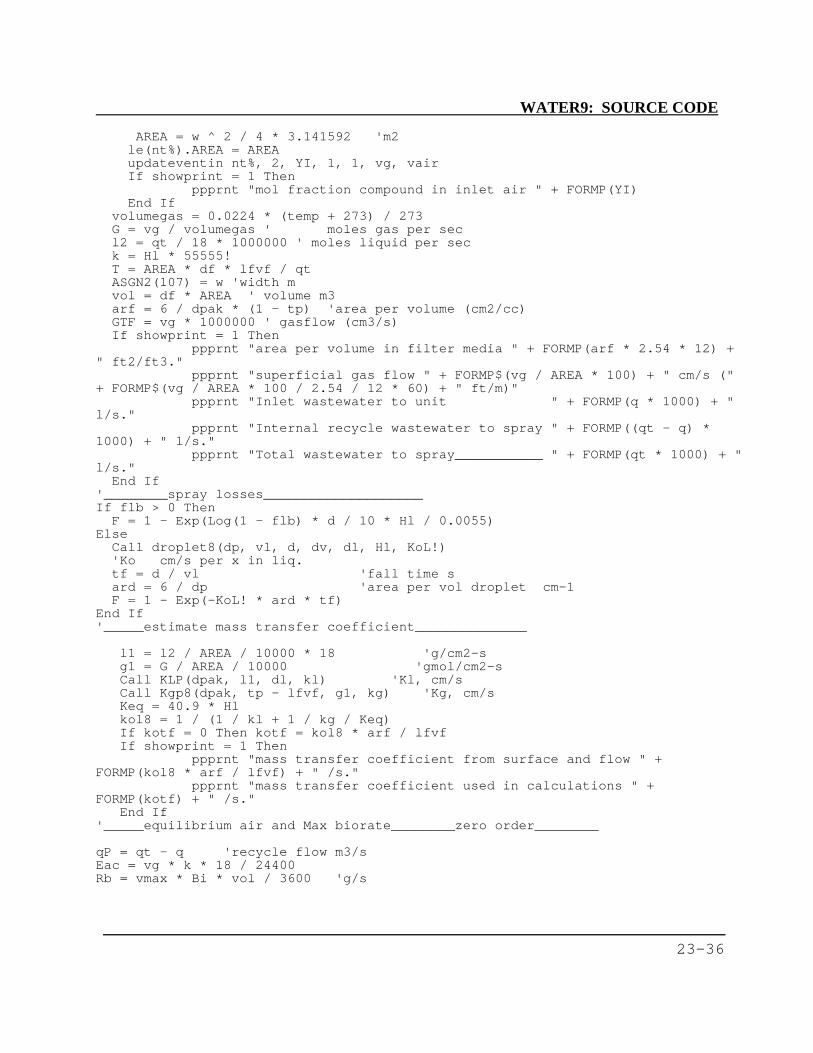
WATER9: SOURCE CODE
23-36
AREA = w ^ 2 / 4 * 3.141592 'm2le(nt%).AREA = AREAupdateventin nt%, 2, YI, 1, 1, vg, vairIf showprint = 1 Then
ppprnt "mol fraction compound in inlet air " + FORMP(YI)End If
volumegas = 0.0224 * (temp + 273) / 273G = vg / volumegas ' moles gas per secl2 = qt / 18 * 1000000 ' moles liquid per seck = Hl * 55555!T = AREA * df * lfvf / qtASGN2(107) = w 'width mvol = df * AREA ' volume m3arf = 6 / dpak * (1 - tp) 'area per volume (cm2/cc)GTF = vg * 1000000 ' gasflow (cm3/s)If showprint = 1 Then
ppprnt "area per volume in filter media " + FORMP(arf * 2.54 * 12) +" ft2/ft3."
ppprnt "superficial gas flow " + FORMP$(vg / AREA * 100) + " cm/s ("+ FORMP$(vg / AREA * 100 / 2.54 / 12 * 60) + " ft/m)"
ppprnt "Inlet wastewater to unit " + FORMP(q * 1000) + "l/s."
ppprnt "Internal recycle wastewater to spray " + FORMP((qt - q) *1000) + " l/s."
ppprnt "Total wastewater to spray___________ " + FORMP(qt * 1000) + "l/s."
End If'________spray losses____________________If flb > 0 Then
F = 1 - Exp(Log(1 - flb) * d / 10 * Hl / 0.0055)Else
Call droplet8(dp, vl, d, dv, dl, Hl, KoL!)'Ko cm/s per x in liq.tf = d / vl 'fall time sard = 6 / dp 'area per vol droplet cm-1F = 1 - Exp(-KoL! * ard * tf)
End If'_____estimate mass transfer coefficient______________
l1 = l2 / AREA / 10000 * 18 'g/cm2-sg1 = G / AREA / 10000 'gmol/cm2-sCall KLP(dpak, l1, dl, kl) 'Kl, cm/sCall Kgp8(dpak, tp - lfvf, g1, kg) 'Kg, cm/sKeq = 40.9 * Hlkol8 = 1 / (1 / kl + 1 / kg / Keq)If kotf = 0 Then kotf = kol8 * arf / lfvfIf showprint = 1 Then
ppprnt "mass transfer coefficient from surface and flow " +FORMP(kol8 * arf / lfvf) + " /s."
ppprnt "mass transfer coefficient used in calculations " +FORMP(kotf) + " /s."
End If'_____equilibrium air and Max biorate________zero order________
qP = qt - q 'recycle flow m3/sEac = vg * k * 18 / 24400Rb = vmax * Bi * vol / 3600 'g/s

WATER9: SOURCE CODE
23-37
If ci > ks And (G * k / l2) < 1 Then' co = (ci * (q - (Eac + Edc) * (1 - f)) - Rb) / ((Eac + Edc) * f)
A11 = q + F * q - (q / qt) * (1 - F)b11 = q + F * qP - Eac * (1 - F) * qP / qtCo = (ci * A11 - Rb) / b11Cip = (1 - rrtf) * ci + rrtf * CoCipp = Cip * (1 - F)If Co > 0.5 * ks Then 'check exit concentration
fair = (Eac * Cipp + F * qt * Cip) / ci / qfbio = Rb / ci / q: fbio3 = fbioGoTo trfilt1
End IfEnd If
'______numerical model___________first order______________xi = ci / aa.mwt / 55555bw = k1 * Bi / lfvf / 3600Call stripper8(G, l2, k, bw, kotf, Nelemen, T, YI, Yo, xi, Xo, fair3, fbio3)
fair = fair3: fbio = fbio3R = rrtf / (1 - rrtf)ftot = F + (1 - F) * (fair + fbio) 'one passIf ftot > 0 Then bioratio = (1 - F) * fbio / ftot Else bioratio = 0sumlost = ftot / (1 + ftot * R) * (1 + R)fbio = bioratio * sumlost: fair = sumlost - fbioCall sumrates8(nt%, fair, fbio, fads, AREA, 0)Call setx1(F, fair3, fbio3, fair, fbio, 0, 0, 0, 0, 0)
If vg > 0 Then cexit = fair * loading / vg 'g/s per m3/sIf (F + fair3) > 0 Then ctop = cexit * fair3 * (1 - F) / (F + fair3 * (1 - F))area_downwind = 1 * wgas_downwind = v / 100 * area_downwind + vg 'm3/sIf showprint = 1 Then
exitconc = ci * (1 - sumlost)loadingwo = exitconc * qbioremoval = fbio * loadingloadingair = YI * G * aa.mwtloadingao = fair * loadingppprnt "____material balance__________________"ppprnt " inlet water (g/s) " + FORMP(loading)ppprnt " inlet air (g/s) " + FORMP(loadingair)ppprnt " bioremoval (g/s) " + FORMP(bioremoval)ppprnt " outlet water (g/s) " + FORMP(loadingwo) + " " + FORMP(exitconc)
+ " g/m3."ppprnt " outlet air (g/s) " + FORMP(loadingao) + " " + FORMP(Yo *
1000000) + " ppmv."ppprnt " SUM material balance (g/s) =" + FORMP(loading + loadingair -
bioremoval - loadingwo - loadingao)ppprnt "____exit concentrations in gas________"ppprnt " mol fraction compound in filter bed " + FORMP(Yo)ppprnt " exit gas concentration over bed " + FORMP(ctop) + " g/m3."ppprnt " avg. undiluted gas concentration over distributor " + FORMP(cexit)
+ " g/m3."If gas_downwind > 0 Then
cdown = fair * loading / gas_downwindarear = fair * loading / AREA 'g/m2-s
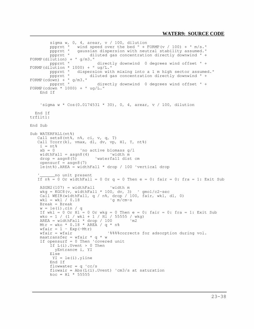
WATER9: SOURCE CODE
23-38
sigma w, 0, 4, arear, v / 100, dilutionppprnt " wind speed over the bed " + FORMP(v / 100) + " m/s."ppprnt " gaussian dispersion with neutral stability assumed."ppprnt " diluted gas concentration directly downwind " +
FORMP(dilution) + " g/m3."ppprnt " directly downwind 0 degrees wind offset " +
FORMP(dilution * 1000) + " ug/L."ppprnt " dispersion with mixing into a 1 m high sector assumed."ppprnt " diluted gas concentration directly downwind " +
FORMP(cdown) + " g/m3."ppprnt " directly downwind 0 degrees wind offset " +
FORMP(cdown * 1000) + " ug/L."End If
'sigma w * Cos(0.0174531 * 30), 0, 4, arear, v / 100, dilution
End Iftrfilt1:
End Sub
Sub WATERFALL(nt%)Call sets8(nt%, n%, ci, v, q, T)Call Tcorr(k1, vmax, dl, dv, vp, Hl, T, nt%)i = nt%xb = 0 'no active biomass g/lwidthFall = asgn8(4) 'width mdrop = asgn8(5) 'waterfall dist cmopensurf = asgn8(7)le(nt%).AREA = widthFall * drop / 100 'vertical drop
'______no unit presentIf n% = 0 Or widthFall = 0 Or q = 0 Then e = 0: fair = 0: fra = 1: Exit Sub
ASGN2(107) = widthFall 'width mwkg = KGC8(v, widthFall * 100, dv, 3) ' gmol/c2-secCall WEIR(widthFall, q / n%, drop / 100, fair, wkl, dl, 0)wkl = wkl / 0.18 'g m/cm-sBreak = Breakw = le(i).cin / qIf wkl = 0 Or Hl = 0 Or wkg = 0 Then e = 0: fair = 0: fra = 1: Exit Subwko = 1 / (1 / wkl + 1 / Hl / 55555 / wkg)AREA = widthFall * drop / 100 'm2Mtr = wko * 0.18 * AREA / q * n%wfair = 1 - Exp(-Mtr)wfair = wfair '%%%%corrects for adsorption during vol.maxtransfer = wfair * q * wIf opensurf = 0 Then 'covered unit
If L(i).Uvent > 0 ThenyEntrance i, YI
ElseYI = le(i).yline
End Ifflowwater = q 'cc/sflowair = Abs(L(i).Uvent) 'cm3/s at saturationkoc = Hl * 55555
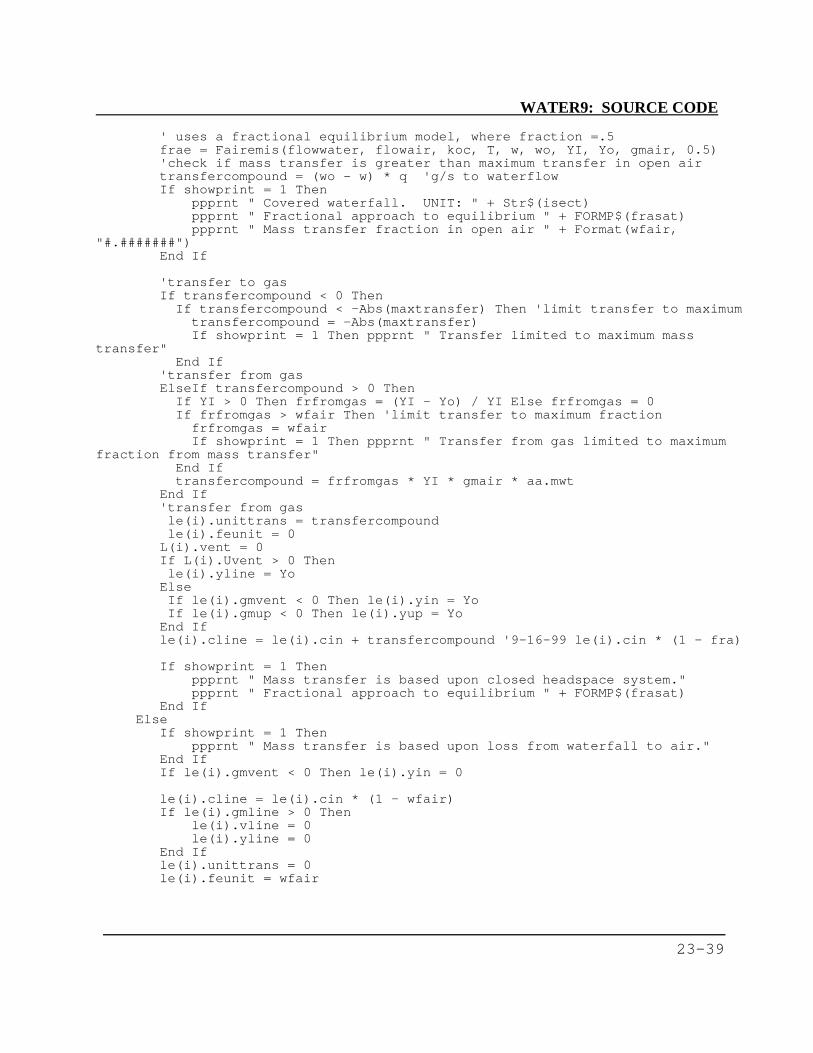
WATER9: SOURCE CODE
23-39
' uses a fractional equilibrium model, where fraction =.5frae = Fairemis(flowwater, flowair, koc, T, w, wo, YI, Yo, gmair, 0.5)'check if mass transfer is greater than maximum transfer in open airtransfercompound = (wo - w) * q 'g/s to waterflowIf showprint = 1 Then
ppprnt " Covered waterfall. UNIT: " + Str$(isect)ppprnt " Fractional approach to equilibrium " + FORMP$(frasat)ppprnt " Mass transfer fraction in open air " + Format(wfair,
"#.#######")End If
'transfer to gasIf transfercompound < 0 Then
If transfercompound < -Abs(maxtransfer) Then 'limit transfer to maximumtransfercompound = -Abs(maxtransfer)If showprint = 1 Then ppprnt " Transfer limited to maximum mass
transfer"End If
'transfer from gasElseIf transfercompound > 0 Then
If YI > 0 Then frfromgas = (YI - Yo) / YI Else frfromgas = 0If frfromgas > wfair Then 'limit transfer to maximum fraction
frfromgas = wfairIf showprint = 1 Then ppprnt " Transfer from gas limited to maximum
fraction from mass transfer"End Iftransfercompound = frfromgas * YI * gmair * aa.mwt
End If'transfer from gasle(i).unittrans = transfercompoundle(i).feunit = 0
L(i).vent = 0If L(i).Uvent > 0 Thenle(i).yline = Yo
ElseIf le(i).gmvent < 0 Then le(i).yin = YoIf le(i).gmup < 0 Then le(i).yup = Yo
End Ifle(i).cline = le(i).cin + transfercompound '9-16-99 le(i).cin * (1 - fra)
If showprint = 1 Thenppprnt " Mass transfer is based upon closed headspace system."ppprnt " Fractional approach to equilibrium " + FORMP$(frasat)
End IfElse
If showprint = 1 Thenppprnt " Mass transfer is based upon loss from waterfall to air."
End IfIf le(i).gmvent < 0 Then le(i).yin = 0
le(i).cline = le(i).cin * (1 - wfair)If le(i).gmline > 0 Then
le(i).vline = 0le(i).yline = 0
End Ifle(i).unittrans = 0le(i).feunit = wfair
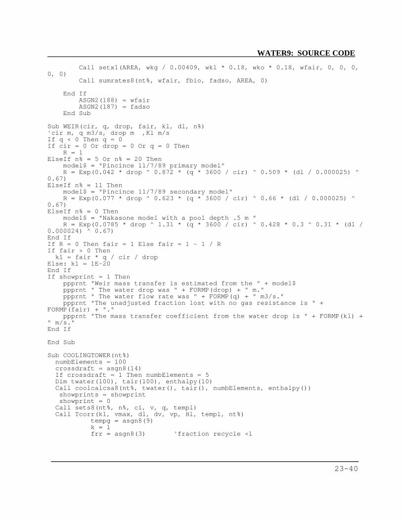
WATER9: SOURCE CODE
23-40
Call setx1(AREA, wkg / 0.00409, wkl * 0.18, wko * 0.18, wfair, 0, 0, 0,0, 0)
Call sumrates8(nt%, wfair, fbio, fadso, AREA, 0)
End IfASGN2(188) = wfairASGN2(187) = fadso
End Sub
Sub WEIR(cir, q, drop, fair, kl, dl, n%)'cir m, q m3/s, drop m ,Kl m/sIf q < 0 Then q = 0If cir = 0 Or drop = 0 Or q = 0 Then
R = 1ElseIf n% = 5 Or n% = 20 Then
model$ = "Pincince 11/7/89 primary model"R = Exp(0.042 * drop ^ 0.872 * (q * 3600 / cir) ^ 0.509 * (dl / 0.000025) ^
0.67)ElseIf n% = 11 Then
model$ = "Pincince 11/7/89 secondary model"R = Exp(0.077 * drop ^ 0.623 * (q * 3600 / cir) ^ 0.66 * (dl / 0.000025) ^
0.67)ElseIf n% = 0 Then
model$ = "Nakasone model with a pool depth .5 m "R = Exp(0.0785 * drop ^ 1.31 * (q * 3600 / cir) ^ 0.428 * 0.3 ^ 0.31 * (dl /
0.000024) ^ 0.67)End IfIf R = 0 Then fair = 1 Else fair = 1 - 1 / RIf fair > 0 Then
kl = fair * q / cir / dropElse: kl = 1E-20End IfIf showprint = 1 Then
ppprnt "Weir mass transfer is estimated from the " + model$ppprnt " The water drop was " + FORMP(drop) + " m."ppprnt " The water flow rate was " + FORMP(q) + " m3/s."ppprnt "The unadjusted fraction lost with no gas resistance is " +
FORMP(fair) + "."ppprnt "The mass transfer coefficient from the water drop is " + FORMP(kl) +
" m/s."End If
End Sub
Sub COOLINGTOWER(nt%)numbElements = 100crossdraft = asgn8(14)If crossdraft = 1 Then numbElements = 5Dim twater(100), tair(100), enthalpy(10)Call coolcalcsa8(nt%, twater(), tair(), numbElements, enthalpy())showprints = showprintshowprint = 0
Call sets8(nt%, n%, ci, v, q, templ)Call Tcorr(k1, vmax, dl, dv, vp, Hl, templ, nt%)
tempg = asgn8(9)k = 1frr = asgn8(3) 'fraction recycle <1
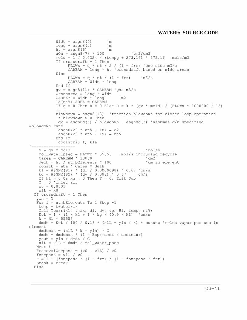
WATER9: SOURCE CODE
23-41
Widt = asgn8(4) 'mleng = asgn8(5) 'mht = asgn8(6) 'maOa = asgn8(7) / 100 'cm2/cm3mold = 1 / 0.0224 / (tempg + 273.16) * 273.16 'mols/m3If crossdraft = 1 Then
FLOWx = q / n% / 2 / (1 - frr) 'one side m3/sCAREAM = leng * ht 'crossdraft based on side areas
ElseFLOWx = q / n% / (1 - frr) 'm3/sCAREAM = Widt * leng
End Ifgv = asgn8(11) * CAREAM 'gas m3/sCrossarea = leng * WidtCAREAM = Widt * leng 'm2le(nt%).AREA = CAREAMIf q = 0 Then R = 0 Else R = k * (gv * mold) / (FLOWx * 1000000 / 18)'----------blowdown = asgn8(13) 'fraction blowdown for closed loop operationIf blowdown > 0 Thenq2 = asgn8d(3) / blowdown - asgn8d(3) 'assumes q/n specified
=blowdown rateasgn8(20 * nt% + 18) = q2asgn8(20 * nt% + 19) = nt%
End If' coolstrip f, kla
'------------------G = gv * mold 'mol/smol_water_psec = FLOWx * 55555 'mol/s including recycleCarea = CAREAM * 10000 'cm2delH = ht / numbElements * 100 'cm in elementconstb = aOa * Carea * delHkl = ASGN2(91) * (dl / 0.0000098) ^ 0.67 'cm/skg = ASGN2(92) * (dv / 0.088) ^ 0.67 'cm/sIf kl = 0 Or kg = 0 Then F = 0: Exit SubY = 0 'inlet airx0 = 0.0001xlL = x0
If crossdraft = 1 Thenyin = YFor i = numbElements To 1 Step -1temp = twater(i)Call Tcorr(k1, vmax, dl, dv, vp, Hl, temp, nt%)KoL = 1 / (1 / kl + 1 / kg / 40.9 / Hl) 'cm/sk = Hl * 55555dmdt = KoL / 100 / 0.18 * (xlL - yin / k) * constb 'moles vapor per sec in
elementdmdtmax = (xlL * k - yin) * Gdmdt = dmdtmax * (1 - Exp(-dmdt / dmdtmax))yout = yin + dmdt / GxlL = xlL - dmdt / mol_water_psec
Next iFremovalOnepass = (x0 - xlL) / x0fonepass = xlL / x0F = 1 - (fonepass * (1 - frr) / (1 - fonepass * frr))Break = Break
Else

WATER9: SOURCE CODE
23-42
For i = 1 To numbElements '10temp = twater(i)Call Tcorr(k1, vmax, dl, dv, vp, Hl, temp, nt%)KoL = 1 / (1 / kl + 1 / kg / 40.9 / Hl) 'cm/sk = Hl * 55555dmdt = KoL / 100 / 0.18 * (xlL - Y / k) * constb 'moles vapor per sec in
elementdmdtmax = (xlL * k - Y) * Gdmdt = dmdtmax * (1 - Exp(-dmdt / dmdtmax))Y = Y + dmdt / GxlL = xlL + dmdt / mol_water_psec
Next ifremoval = (xlL - x0) / xlLfonepass = x0 / xlLF = 1 - (fonepass * (1 - frr) / (1 - fonepass * frr))
End Ifshowprint = showprintsIf showprint = 1 Then
ppprnt "__Temperatures in the cooling tower at various heights"ppprnt " height temperature air temperature water"ppprnt " (m) (C) (C)"If crossdraft = 1 Then stepsize = -1 Else stepsize = -5For ik = numbElements To 1 Step stepsize
datasets$ = String(80, 32)Mid$(datasets$, 5) = FORMP(delH / 100 * ik)Mid$(datasets$, 20) = Format(tair(ik), "###.##")Mid$(datasets$, 42) = Format(twater(ik), "###.##")ppprnt datasets$
Nextppprnt "__Overall mass and heat flows____________________"ppprnt "Mass flow rate of air (gmol/s) " + FORMP(G)ppprnt "Mass flow rate of water (gmol/s) " + FORMP(mol_water_psec)ppprnt "Moles water evaporation (gmol/s) " + FORMP(enthalpy(3))ppprnt "Percent of water evaporated per pass " + Format(enthalpy(3) /
mol_water_psec, "##.### %")ppprnt "Heat of evaporation from water (cal/s) " + FORMP(enthalpy(1))ppprnt "Heat gain in air (cal/s) " + FORMP(enthalpy(4))ppprnt "Heat gain water transfer to air (cal/s) " + FORMP(enthalpy(6))ppprnt "Heat loss from from water (cal/s) " + FORMP(enthalpy(5))ppprnt "heat balance " + Format((-enthalpy(4) +
enthalpy(5) - enthalpy(1)) / enthalpy(5), "###.## %")ppprnt " "
End Ifkla = KoL * aOa '/s
'------------------FR = 1 - F 'fract remain
Call setx1(kl / 100, kg / 100, KoL / 100, kla, ASGN2(291), enthalpy(2),ASGN2(279), F, 0, 0)
Call sumrates8(nt%, F, 0, 0, CAREAM, 0)
End Sub
Public Sub clarifierRec(nt%)Call sets8(nt%, n%, ci, v, q, T)Call Tcorr(k1, vmax, dl, dv, vp, Hl, T, nt%)

WATER9: SOURCE CODE
23-43
xb = 0 'no active biomass g/ldepth = asgn8(3) 'flow depth cm
d = asgn8(4) 'Depth meff = asgn8(5) 'effectiveness solids removalwl = asgn8(6) 'waterfall dist cmww = asgn8(7) 'width overflow mLng = asgn8(8) 'length mw = asgn8(9) 'width m
totalin nt%, sumSolids, sumBiomass, sumOil, sumDiss 'g/ssolids = L(nt%).sludge 'suspended solids mg/l
' fremsusp(nt%) = eff %%%%controlf = asgn8(15)ventperarea = asgn8(16) 'm3/s per m2 areacover% = asgn8(17)
If cover% = 1 Thenv = ventperarea * 200 'cm/s 0.5 meter depthIf showprint = 1 Then
ppprnt "The retangular clarifier has a cover."ppprnt "A headspace distance of 50 cm is assumed under the cover."ppprnt "The gas flow rate is " + FORMP(v) + " cm/s based on 200 * the
vent rate per area " + FORMP(ventperarea) + " m3/s per m2"Call printprop2(k1, vmax, dl, dv, vp, Hl, T)
End IfEnd IfIf n% = 0 Or q = 0 Then e = 0: fair = 0: fra = 1: Exit Sub 'no unit present
ASGN2(107) = w 'width mIf cover% = 1 Then ASGN2(107) = 0.33SAREA = Lng * w 'm2ventrate = SAREA * ventperareale(nt%).AREA = SAREA
'________emissions from clarifier surface_____ksl = 10 ^ (0.67 * aa.low - 2.61) + 0.099 'g/m3 per g/Kg biomassfadso = solids * ksl / (solids * ksl + 1000) 'fraction sorbedflowwater = q * 1000000 / n%
Call TRENCHS(flowwater, depth, w * 100, dl, kl)' model for flow in junction box dl cm2/s' flowwwater cm3/s depth cm wid cm Kl m/s
restime = SAREA * d / q * n% 'svcl = w / 2 / restime * 100 'water vel, cm/sskg = KGC8(v, Lng * 100, dv, 3) 'open gm/c2-sIf kl = 0 ThenMsgBox "kl = 0, a default of 1e-20 is assumed"kl = 1E-20
End Ifskl = kl / 0.18 'gm/c2-ssko = 1 / (1 / skl + 1 / (Hl * (1 - fadso)) / 55555 / skg) 'gm/c2-sMtr = sko * 0.18 / d * restimeIf showprint = 1 Then
ppprnt "The residence time in the clarifier is " + Format$(restime /3600, "###.###") + " hrs."
ppprnt "The Henry's law constant of " + FORMP(Hl) + " atm-m3/mol ismultiplied by"
ppprnt " a adsorption factor of " + FORMP(1 - fadso) + "."ppprnt "The gas phase mass transfer is estimated using correlation 3,
MacKay (1983)."ppprnt "Gas phase mass transfer " + FORMP(skg) + " g mol/ cm2-s."
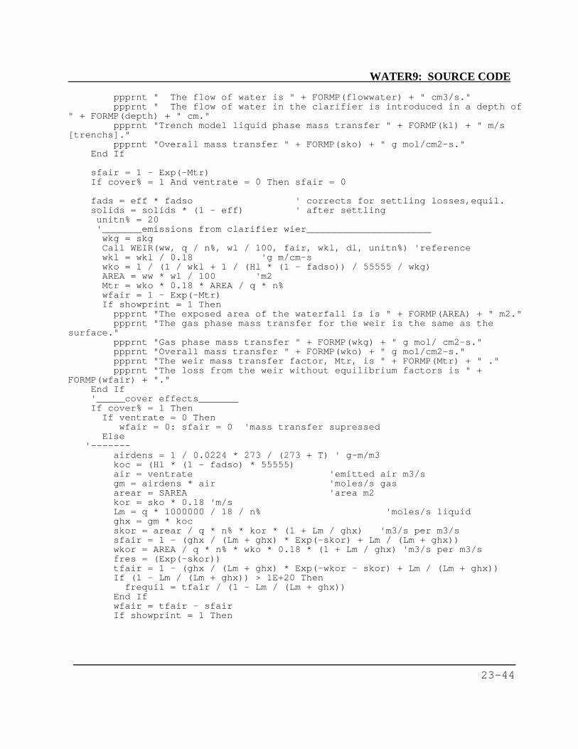
WATER9: SOURCE CODE
23-44
ppprnt " The flow of water is " + FORMP(flowwater) + " cm3/s."ppprnt " The flow of water in the clarifier is introduced in a depth of
" + FORMP(depth) + " cm."ppprnt "Trench model liquid phase mass transfer " + FORMP(kl) + " m/s
[trenchs]."ppprnt "Overall mass transfer " + FORMP(sko) + " g mol/cm2-s."
End If
sfair = 1 - Exp(-Mtr)If cover% = 1 And ventrate = 0 Then sfair = 0
fads = eff * fadso ' corrects for settling losses,equil.solids = solids * (1 - eff) ' after settlingunitn% = 20'_______emissions from clarifier wier______________________wkg = skgCall WEIR(ww, q / n%, wl / 100, fair, wkl, dl, unitn%) 'referencewkl = wkl / 0.18 'g m/cm-swko = 1 / (1 / wkl + 1 / (Hl * (1 - fadso)) / 55555 / wkg)AREA = ww * wl / 100 'm2Mtr = wko * 0.18 * AREA / q * n%wfair = 1 - Exp(-Mtr)If showprint = 1 Then
ppprnt "The exposed area of the waterfall is is " + FORMP(AREA) + " m2."ppprnt "The gas phase mass transfer for the weir is the same as the
surface."ppprnt "Gas phase mass transfer " + FORMP(wkg) + " g mol/ cm2-s."ppprnt "Overall mass transfer " + FORMP(wko) + " g mol/cm2-s."ppprnt "The weir mass transfer factor, Mtr, is " + FORMP(Mtr) + " ."ppprnt "The loss from the weir without equilibrium factors is " +
FORMP(wfair) + "."End If'_____cover effects_______If cover% = 1 Then
If ventrate = 0 Thenwfair = 0: sfair = 0 'mass transfer supressed
Else'-------
airdens = 1 / 0.0224 * 273 / (273 + T) ' g-m/m3koc = (Hl * (1 - fadso) * 55555)air = ventrate 'emitted air m3/sgm = airdens * air 'moles/s gasarear = SAREA 'area m2kor = sko * 0.18 'm/sLm = q * 1000000 / 18 / n% 'moles/s liquidghx = gm * kocskor = arear / q * n% * kor * (1 + Lm / ghx) 'm3/s per m3/ssfair = 1 - (ghx / (Lm + ghx) * Exp(-skor) + Lm / (Lm + ghx))wkor = AREA / q * n% * wko * 0.18 * (1 + Lm / ghx) 'm3/s per m3/sfres = (Exp(-skor))tfair = 1 - (ghx / (Lm + ghx) * Exp(-wkor - skor) + Lm / (Lm + ghx))If (1 - Lm / (Lm + ghx)) > 1E+20 Then
frequil = tfair / (1 - Lm / (Lm + ghx))End Ifwfair = tfair - sfairIf showprint = 1 Then
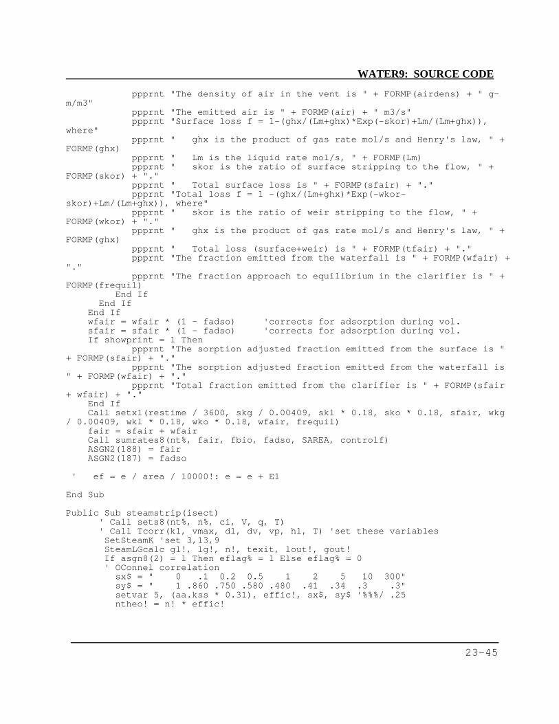
WATER9: SOURCE CODE
23-45
ppprnt "The density of air in the vent is " + FORMP(airdens) + " g-m/m3"
ppprnt "The emitted air is " + FORMP(air) + " m3/s"ppprnt "Surface loss f = 1-(ghx/(Lm+ghx)*Exp(-skor)+Lm/(Lm+ghx)),
where"ppprnt " ghx is the product of gas rate mol/s and Henry's law, " +
FORMP(ghx)ppprnt " Lm is the liquid rate mol/s, " + FORMP(Lm)ppprnt " skor is the ratio of surface stripping to the flow, " +
FORMP(skor) + "."ppprnt " Total surface loss is " + FORMP(sfair) + "."ppprnt "Total loss f = 1 -(ghx/(Lm+ghx)*Exp(-wkor-
skor)+Lm/(Lm+ghx)), where"ppprnt " skor is the ratio of weir stripping to the flow, " +
FORMP(wkor) + "."ppprnt " ghx is the product of gas rate mol/s and Henry's law, " +
FORMP(ghx)ppprnt " Total loss (surface+weir) is " + FORMP(tfair) + "."ppprnt "The fraction emitted from the waterfall is " + FORMP(wfair) +
"."ppprnt "The fraction approach to equilibrium in the clarifier is " +
FORMP(frequil)End If
End IfEnd Ifwfair = wfair * (1 - fadso) 'corrects for adsorption during vol.sfair = sfair * (1 - fadso) 'corrects for adsorption during vol.If showprint = 1 Then
ppprnt "The sorption adjusted fraction emitted from the surface is "+ FORMP(sfair) + "."
ppprnt "The sorption adjusted fraction emitted from the waterfall is" + FORMP(wfair) + "."
ppprnt "Total fraction emitted from the clarifier is " + FORMP(sfair+ wfair) + "."
End IfCall setx1(restime / 3600, skg / 0.00409, skl * 0.18, sko * 0.18, sfair, wkg
/ 0.00409, wkl * 0.18, wko * 0.18, wfair, frequil)fair = sfair + wfairCall sumrates8(nt%, fair, fbio, fadso, SAREA, controlf)ASGN2(188) = fairASGN2(187) = fadso
' ef = e / area / 10000!: e = e + E1
End Sub
Public Sub steamstrip(isect)' Call sets8(nt%, n%, ci, V, q, T)' Call Tcorr(k1, vmax, dl, dv, vp, hl, T) 'set these variablesSetSteamK 'set 3,13,9SteamLGcalc gl!, lg!, n!, texit, lout!, gout!If asgn8(2) = 1 Then eflag% = 1 Else eflag% = 0' OConnel correlation
sx$ = " 0 .1 0.2 0.5 1 2 5 10 300"sy$ = " 1 .860 .750 .580 .480 .41 .34 .3 .3"setvar 5, (aa.kss * 0.31), effic!, sx$, sy$ '%%%/ .25ntheo! = n! * effic!
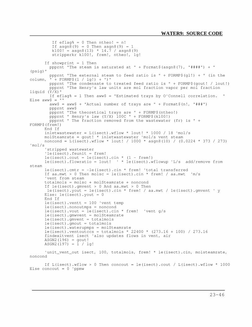
WATER9: SOURCE CODE
23-46
If eflag% = 0 Then ntheo! = n!If asgn8(9) = 0 Then asgn8(9) = 1k100! = asgn8(13) * 14.7 / asgn8(9)stripperkr k100!, frem!, ntheo!, lg!
If showprint = 1 Thenppprnt "The steam is saturated at " + Format$(asgn8(7), "####") + "
(psig)"ppprnt "The external steam to feed ratio is " + FORMP$(gl!) + " (in the
column, " + FORMP$(1 / lg!) + ")"ppprnt "The condensate to treated feed ratio is " + FORMP$(gout! / lout!)ppprnt "The Henry's law units are mol fraction vapor per mol fraction
liquid (Y/X)"If eflag% = 1 Then aww$ = "Estimated trays by O'Connell correlation. "
Else aww$ = ""aww$ = aww$ + "Actual number of trays are " + Format$(n!, "###")ppprnt aww$ppprnt "The theoretical trays are " + FORMP$(ntheo!)ppprnt " Henry's law (Y/X) 100C " + FORMP$(k100!)ppprnt " The fraction removed from the wastewater (fr) is " +
FORMP$(frem!)End Ifinletwastewater = L(isect).wflow * lout! * 1000 / 18 'mol/smolSteamrate = gout! * inletwastewater 'mol/s vent steamnoncond = L(isect).wflow * lout! / 1000 * asgn8(10) / (0.0224 * 373 / 273)
'mol/s'stripped wastewater'le(isect).feunit = frem!le(isect).cout = le(isect).cin * (1 - frem!)le(isect).flowratio = lout! ' * le(isect).wflowup 'L/s add/remove from
steamle(isect).cmtr = -le(isect).cin * frem! 'total transferredIf aa.mwt > 0 Then molsc = le(isect).cin * frem! / aa.mwt 'm/s'vent from steamtotalmols = molsc + molSteamrate + noncondIf le(isect).gmvent > 0 And aa.mwt > 0 Thenle(isect).yout = le(isect).cin * frem! / aa.mwt / le(isect).gmvent ' y
Else: le(isect).yout = 0End Ifle(isect).ventt = 100 'vent temple(isect).nonoutmps = noncondle(isect).vout = le(isect).cin * frem! 'vent g/sle(isect).gmwvent = molSteamratele(isect).gmvent = totalmolsle(isect).gmout = totalmolsle(isect).waterupmps = molSteamratele(isect).ventoutccs = totalmols * 22400 * (273.16 + 100) / 273.16findexitvent isect 'also updates flows in vent, airASGN2(196) = gout!ASGN2(197) = 1 / lg!
'unit_vent_out isect, 100, totalmols, frem! * le(isect).cin, molsteamrate,noncond
If L(isect).wflow > 0 Then concout = le(isect).cout / L(isect).wflow * 1000Else concout = 0 'ppmw
WATER9: SOURCE CODE
23-47
If molSteamrate > 0 Then noncondc = noncond / molSteamrate Else noncondc =0
Call setx1(gl!, ntheo!, 100, 0, concout, molSteamrate, 100, noncondc,le(isect).yvent * 1000000, frem!) '2-11 asgn2(172-
End Sub
Public Sub packedair(nt%, mpswater, cwater, cgas, Gmps)Call sets8(nt%, n%, ci, v, q, temp)If q = 0 Or n% = 0 Then Exit Subq = q / n% 'corrects for number of units
'Lmps liquid (m3/s)'Gmps gas inlet (m3/s)'q inlet flow rate waste (m3/s)'temp Wastewater temperature (C)'ci,cwater inlet conc (mg/l in)'n% packed air modules, number units
If mpswater > 0 Then q = mpswaterIf cgas > 0 Then YI = cgas Else YI = le(nt%).yupairdens = 1 / 0.0224 * 273 / (273 + temp) ' g-m/m3If Gmps = 0 Then Gmps = le(nt%).gmup / airdensIf cwater > 0 Then ci = cwater 'overwrites actualdp = asgn8(11) 'Droplet diameter of spray (cm)d = asgn8(10) 'Droplet fall (cm)
flb = asgn8(12) 'Spray fractional loss,BENZENE (10 cm)If aa.k1 > 0 Then ks = aa.biov / aa.k1 Else ks = 1Call Tcorr(k1, vmax, dl, dv, vp, Hl, temp, nt%)df = asgn8(7) ' depth (m)
kotf = asgn8(9) ' Mass transfer coef bed (/sec)dia = asgn8(14) ' packed bed diameter (m)
rrtf = asgn8(15) ' internal recycle ratiolfvf = asgn8(4) ' Liquid hold-up (volume fraction)
Bi = asgn8(13) ' biomass in packed bed (g/l)dpak = asgn8(3) 'packing diameter cm
tp = asgn8(5) ' bed porosityIf rrtf > 0.99 Then rrtf = 0.99If dpak = 0 Then dpak = 1 '%%Nelemen = 100 'df * 100 / dpak 'filter elementsIf Nelemen > 75 Then Nelemen = 75If tp = 0 Then tp = 0.5qt = q / (1 - rrtf) ' corrects for recycle and unitsvg = Gmps ' Gas flow (m3/s)If vg = 0 Then Exit SubAREA = dia ^ 2 / 4 * 3.141592 'm2sgv = vg / AREA 'm3/s per m2le(nt%).AREA = AREAIf aa.mwt = 0 Then aa.mwt = 100
xi = ci / aa.mwt / 55555xiinit = xiG = Gmps * airdens ' moles gas per seclm1 = q / 18 * 1000000l2 = qt / 18 * 1000000 ' moles liquid per secmoleratio = G / l2volratio = Gmps / qtk = Hl * 55555!T = AREA * df * lfvf / qt 'holdup time sec
WATER9: SOURCE CODE
23-48
ASGN2(107) = Sqr(w * Length) 'width mvol = df * AREA ' volume m3arf = 6 / dpak * (1 - tp) 'area per volume (cm2/cc)GTF = vg * 1000000 ' gasflow (cm3/s)
'________spray losses____________________If flb > 0 Then
F = 1 - Exp(Log(1 - flb) * d / 10 * Hl / 0.0055)Else
Call droplet8(dp, vl, d, dv, dl, Hl, KoL!)'Ko cm/s per x in liq.If vl > 0 And dp > 0 Thentf = d / vl 'fall time sard = 6 / dp 'area per vol droplet cm-1
Else:tf = 0ard = 0
End If
F = 1 - Exp(-KoL! * ard * tf)End If'_____estimate mass transfer coefficient______________
If AREA > 0 Thenl1 = l2 / AREA / 10000 * 18 'g/cm2-sg1 = G / AREA / 10000 'gmol/cm2-s
ElseExit Sub
End IfCall KLP(dpak, l1, dl, kl) 'Kl, cm/sCall Kgp8(dpak, tp - lfvf, g1, kg) 'Kg, cm/sKeq = 40.9 * Hlkol8 = 1 / (1 / kl + 1 / kg / Keq)If kotf = 0 Then kotf = kol8 * arf / lfvf
'_____equilibrium air and Max biorate________zero order________
qP = qt - q 'recycle flow m3/sEac = vg * k * 18 / 24400Rb = vmax * Bi * vol / 3600 'g/sIf ci > ks And (G * k / l2) < 1 Then' co = (ci * (q - (Eac + Edc) * (1 - f)) - Rb) / ((Eac + Edc) * f)
A11 = q + F * q - (q / qt) * (1 - F)b11 = q + F * qP - Eac * (1 - F) * qP / qtCo = (ci * A11 - Rb) / b11Cip = (1 - rrtf) * ci + rrtf * CoCipp = Cip * (1 - F)If Co > 0.5 * ks Then 'check exit concentration
fair = (Eac * Cipp + F * qt * Cip) / ci / qfbio = Rb / ci / q: fbio3 = fbioGoTo trfilt11
End IfEnd If
'______numerical model___________first order______________bw = k1 * Bi / lfvf / 3600For iter = 1 To 20

WATER9: SOURCE CODE
23-49
xold = xiCall stripper(G, l2, k, bw, kotf, Nelemen, T, YI, Yo, xi, Xo, fair3, fbio3,
cmtr)If (Yo < YI) Then 'g/s added mass transfer from gas to liquid
le(nt%).unittrans = (-Xo + xi) * lm1 * aa.mwt 'g/sElse
le(nt%).unittrans = 0End Ifxnew = (xiinit * (1 - rrtf) + Xo * rrtf) * (1 - F)xi = xold * 0.5 + xnew * 0.5
Nextfair = fair3fbio = fbio3R = rrtf / (1 - rrtf)ftot = F + (1 - F) * (fair + fbio)If ftot > 0 Thenbioratio = (1 - F) * fbio / ftot 'bioremoval/total removalElse: bioratio = 0End Ifsumlost = ftot / (1 + ftot * R) * (1 + R)fbio = bioratio * sumlostfair = sumlost - fbioIf YI > 0 Then fgrem = (YI - Yo) / YI Else fgrem = 0
trfilt11:'correct yo for spray lossYo = (Yo * G + xi * l2 * F) / GIf YI > 0 Then fyair = (YI - Yo) / YI Else fyair = 0If (l2 * xi + G * YI) = 0 Or bw = 0 Then 'no inlet concentrations
tfbio = 0Else
tfbio = ((lm1 * xiinit + G * YI) - (lm1 * Xo + G * Yo)) / (lm1 * xiinit + G *YI)
End IfCall setx1(F, fair3, fbio3, fair, fbio, kotf, Yo, Xo, fyair, tfbio)le(nt%).yout = Yole(nt%).gmout = Gle(nt%).vout = G * Yo * aa.mwtle(nt%).ventt = tempBreak = Break
If showprint = 1 Thenppprnt "The ratio of gas to liquid is " + Format$(moleratio, "####.####") + "
mol ratio; " + Format$(volratio, "####.####") + " vol ratio"ppprnt "The surface area per volume of the bed is " + Str$(arf) + " (cm2/cc)."ppprnt "The superficial gas velocity is " + Str$(sgv) + " (m/s)."ppprnt "The effective biomass in the bed is " + Format$(Bi, "##.###### g/L")
'mg /cm2ppprnt "The bioremoval fraction (material balance) is " + Format$(tfbio,
"#.######")ppprnt "The mol fraction in the inlet gas is " + Format$(YI, "#.###e+00")ppprnt "The mol fraction in the outlet gas is " + Format$(Yo, "#.###e+00")ppprnt "The mol fraction in the inlet liquid is " + Format$(xi, "#.###e+00")ppprnt "The mol fraction in the outlet liquid is " + Format$(Xo, "#.###e+00")ppprnt "The fractional removal of compound fron the inlet gas is " +
Format$(fgrem, "#.###e+00")ppprnt "The exit gas rate is " + Format$(Yo * G * aa.mwt, "#.###e+00") + "
g/s."

WATER9: SOURCE CODE
23-50
End Ifcout = Xo * l2 * (1 - rrtf) * aa.mwtle(nt%).cline = cout 'g/s liquidle(nt%).cout = cout 'g/s liquidle(nt%).feline = 0le(nt%).crem = tfbio * (ci * q + YI * G * aa.mwt)le(nt%).fbio = tfbiole(nt%).fsludge = 0le(nt%).foil = 0If Xo > xiinit Then
le(nt%).unittrans = lm1 * (Xo - xiinit) * aa.mwtle(nt%).feunit = 0
Elsele(nt%).unittrans = 0le(nt%).feunit = fair
End Ifle(nt%).eunit = 0le(nt%).vout = Yo * G * aa.mwtle(nt%).e = 0ASGN2(179) = XoASGN2(180) = fgremASGN2(181) = tfbioASGN2(178) = Yofindexitvent isect 'also updates flows in vent, airEnd Sub
Public Sub poroussol(isect)'44 and 45' nn% is the munber of the compound in the tagged set' time days after initial time' e air emissions, g/sec.' Wid is the width of the plot (cm)nn% = isectCall sets8(nn%, n%, ci, v, q, T)Call Tcorr(k1, vmax, dl, dv, vp, Hl, T, nn%)TimeExp = asgn8(7)ea = asgn8(5) 'air porosityet = asgn8(4) 'Total porosityk = Hl * 55555
wasteflow = L(isect).wflow * 1000 'g/s wasteoilflow = L(isect).oil 'g/ssolidflow = L(isect).solids 'g/sIf wasteflow = 0 Then
Call setx8(0, 0, 0, 0, 0, 0, 0) ' 13-19Call sumrates8(nn%, 0, 0, 0, ta, 0)Exit Sub
End Ifoilfract = oilflow / wasteflow 'weight fraction oil in wastesolidfract = solidflow / wasteflow 'weight fraction solids in wastewfwater = (wasteflow - solidflow - oilflow) / wasteflow 'weight fraction water
in liquidcompflow = le(isect).cin 'g/sppmw = compflow / wasteflow * 1000000 'compound mg/l in waste
WATER9: SOURCE CODE
23-51
ppmwo = compflow / wasteflow / (1 - solidfract) * 1000000 'compound mg/l inliquid
el = et - ea: If el <= 0 Then el = 0.1 'defaultrhol = 0.9
' timetofill = volume * el * rhol / wasteflow / 3600 / 24 / 365.25 * 12 'months' solidmass = volume * (1 - et) * 2 / 1000 'default solid density=2 g/cc' wastemass = solidflow / 1000 * timetofill * 3600 * 24 * 365.25 / 12 'kg' stabilize = (solidmass - wastemass) / timetofill 'kg/month
Call fractionoil(oilfract, owpc, owr, frinoil, 0)
aqfg = asgn(79) 'aqueous flag: organic waste, =1; aqueous waste, =0mwt = aa.mwt 'molecular weight of constituentmwtl = asgn8(6) 'molecular weight of solventtk = T + 273.16 'temperature in soil, deg KelvinR = 82.05 'atm-cm3/g mol-kc = asgn8(9) 'waste in matrix g/cm3oilload = c * oilfract 'oil in matrix g/cm3de = difvv(dv, et, ea, 1) 'diffusivity in soil (cm2/s)Lz = asgn8(3) 'depth of contamination cmIf Lz = 0 Then Exit SubMo = c * Lz * ppmw / 1000000! 'loading g constituent/cm2 soil surfaceCo = Mo / Lzbz = asgn8(8) 'g/l biomass densityAREA = asgn8(11) * 10000 'cm2wid = (AREA) ^ 0.5 'cm
' mass transfer at surface of soil, cm/skg = KGC8(v, wid, dv, 2) * 240 * 100 'cm/sIf bz < 1E-30 Or vmax < 1E-30 Then
tb = 10000000000#Else:'based upon .01 g/cc biomass conc.tb = 86400! * 5.58823 / bz / vmax 'rate const. biological, (s)End If
' calculate temperature correction factor for vapor pressure' If ac.b < 1 Then ac.b = 1000: ac.c = 273.16' vpref = Exp((-ac.b / (25 + ac.c)) * 2.302528)' vpspec = Exp((-ac.b / (asgn8(9) + ac.c)) * 2.302528)' Tcorr = vpspec / vpref' If asgn(79) = 0 Then 'aqueous flag: organic waste, =1; aqueous waste, =0' keq = Tcorr * ac.vp / 760 * MWoil / r / Tk * ea / asgn(75) 'solvent is
oil' Else: keq = Tcorr * ac.hl * 1000000! / r / Tk * ea / asgn(75) 'solvent is
water' End IfIf mwt = 0 Then mwt = 100If frinoil < 0.2 Then 'aqueous
cw = compflow * (1 - frinoil) / wasteflow / wfwater ' ppmw in waterXz = cw / ((1000000 - cw) * mwt / 18 + cw) 'mole fract in waterkr = kY = kr * XzIf c = 0 Then Exit Sub'keq = kr * ea / r / tk / c 'ratio comp in gas/comp in porous solidsgv = ea / R / tkKeq = kr * gv / (kr * gv + c / 18)Oilywaste = 0
Else 'oily
WATER9: SOURCE CODE
23-52
coil = compflow * frinoil / wasteflow / oilfract * 1000000 'ppmw in oilXz = coil / ((1000000 - coil) * mwt / mwtl + coil)kr = vp / 760Y = Xz * krgv = ea / R / tkKeq = kr * gv / (kr * gv + oilload / mwtl) 'ratio comp in gas/comp in porous
solidsOilywaste = 1
End If' cs = concvapor(kr, MWT, Xz, T) 'g/cc
keqdef = 0.0002106If Keq <= 0 Then Keq = keqdef'___________
'T = 8! * 3600!: GoSub landtreat1: X(4) = e ' 8 hr calculation'T = 15! * 60!: GoSub landtreat1: X(5) = einst '15 min calculationTms = TimeExp * 24 * 3600 'sec 'time specified calculation
Kv = Keq * de / Lz / LzZ2 = Tms / tbKd = Pi * Pi / 4 * KvKvT = Kv * TmsKvTb = Kv * tbKdTb = Kd * tbKdt = Kd * Tms
' instantaneous emissionsIf KvT < 0.213 Then
e = Mo / Lz / (ea / Keq / kg + (Pi * Tms / de / Keq) ^ 0.5) * Exp(-Z2)'g/cm2-s
Else: e = Mo * (2 * Kv) * Exp(-Kdt - Z2)End Ifeinst = e * AREA 'g/cm2-s*cm2 >> g/s
' average emissionsIf KdTb > 0.62 Then
fa = 0.811 * KdTb / (KdTb + 1) + 0.1878Else: fa = (KvTb) ^ 0.5End Ifltfbio = 1 - faIf fa < 0.33 Then
'Fatp = Fa * (1 - EXP(-Kdt))Fatp = (KvT / Pi) ^ 0.5 * 2: gerf = 1fat = fa * (1 - Exp(-Kdt - Z2))
ElseIf KvT > 0.22 ThenFatp = 8 / Pi / Pi * (1 - Exp(-Kdt)) + 0.1878: gerf = 2fat = 8 / Pi / Pi / (1 + 1 / KdTb) * (1 - Exp(-Kdt - Z2)) + 0.1878
ElseFatp = (KvT / Pi) ^ 0.5 * 2: gerf = 3fat = Fatp * (1 - 1 / 3 * Z2)
End Iffremain = (1 - Fatp) * Exp(-Z2)fbio = 1 - fat - fremain:If fbio > (1 - fa) Then fbio = (1 - fa): fremain = 1 - fat - fbioe = fat * AREA * Mo / Tmsfair = fat
If showprint = 1 ThenIf Oilywaste = 0 Thenppprnt "Aqueous waste characteristics are assumed."

WATER9: SOURCE CODE
23-53
Elseppprnt "Oily waste characteristics and Raoult's law are assumed."End Ifppprnt "The waste loading is " + Format$(c, "##.####") + " g/cc."ppprnt "The oil loading is " + Format$(oilload, "##.####") + " g/cc."ppprnt "The area of the unit is " + Str$(AREA) + " cm2."ppprnt "The instantaneous rate is " + Format$(einst, "##.###### g/s")ppprnt "The long term bioremoval fraction is " + Format$(ltfbio, "#.######")
End If'192,191Call setx1(Keq, tb, de, 1 - fa, fremain, fat, (1 - fbio - fat) * ppmwo, fbio,
einst, oilload) '2-11Call setx8(0, 0, 0, fair, fbio, 0, fads) ' 13-19Call sumrates8(nn%, fair, fbio, fads, ta, 0)le(isect).e = fair * le(isect).cinle(isect).AREA = AREA / 10000 'm2le(isect).cremain = le(isect).cin * fremainle(isect).cout = 0 'le(isect).cin * fremainle(isect).crem = le(isect).cin * fbio
End Sub
Public Sub fill(isect)mwt = aa.mwttemp = asgn8(2)
ea = asgn8(4)et = asgn8(5)AREA = asgn8(6) * 10000 'cm2porl = asgn8(7) 'air porosity in wastedelp = asgn8(8) 'mbardeltemp = asgn8(9) 'change in ref.temperature with diurnal changetimeperiod = asgn8(10) 'time for barometric pumping sec.oilinL = asgn8(11) 'fraction oil in liquid after stabilizationrhol = asgn8(12) 'waste liquid in waste after stabilization g/ccmwtl = asgn8(13)timexp = asgn8(14) * 2629800! 'secd = asgn8(15) * 100 'depth (cm)volg = asgn8(16) 'cc gas per g convertedbiomass = asgn8(17) 'g/cctotalbiorate = asgn8(18) 'mg/g bio-hrvolume = AREA * d 'ccle(isect).AREA = asgn8(6) 'm2
wasteflow = L(isect).wflow * 1000 'g/s wasteoilflow = L(isect).oilsolidflow = L(isect).solidsIf wasteflow = 0 Then Exit Suboilfract = oilflow / wasteflow 'weight fraction oil in wastesolidfract = solidflow / wasteflow 'weight fraction solids in wastewfwater = (wasteflow - solidflow - oilflow) / wasteflow 'weight fraction water
in liquidcompflow = le(isect).cinc = compflow / wasteflow / (1 - solidfract) 'compound mg/l in liquidCo = rhol * compflow / wasteflow 'g/cc in wasteel = et - ea: If el <= 0 Then el = 0.1 'defaulttimetofill = volume * rhol / wasteflow / 3600 / 24 / 365.25 * 12 'months

WATER9: SOURCE CODE
23-54
If timetofill = 0 Then Exit Subsolidmass = volume * 2 / 1000000 'Mg, default solid density=2 g/ccwastemass = solidflow / 1000000 * timetofill * 3600 * 24 * 365.25 / 12 'Mgstabilize = (solidmass - wastemass) / timetofill 'Mg/monthIf aa.k1 > 0 Then ks = aa.biov / aa.k1 Else ks = 0nt% = isectCall Tcorr(k1, vmax, dl, dv, vp, Hl, temp, nt%)Call fractionoil(oilfract, owpc, owr, frinoil, 0)
k = Hl * 55555total = volume * Co 'total grams volatile compound in landfillR = 82.05 'cc-atm/mol-deg Kdvf = difvv(dv, et, ea, 1)If mwt < 2 Then mwt = 100 'defaultIf frinoil < 0.5 Then 'aqueous present
c = compflow * (1 - frinoil) / wasteflow / wfwater * 1000000 ' ppmw in waterXz = c / ((1000000 - c) * mwt / 18 + c)kr = kY = kr * Xz
Else 'oilyc = compflow * frinoil / wasteflow / oilfract * 1000000 'ppmw in oilIf mwt < 2 Then mwt = 100Xz = c / ((1000000 - c) * mwt / mwtl + c)kr = vp / 760Y = Xz * kr
End If
cs = concvapor(kr, mwt, Xz, temp) 'g/cc
'caq is ratio of mg/l in water to g/cc aircaq = R * (temp + 273.16) / 18 / k * 1000000
'rates of release in cc/secgasrate = volg * biomass * volume * totalbiorate / 1000 / 3600If (ks + caq * cs) > 0 Then
biorate1 = vmax * biomass * volume * caq / (ks + caq * cs) / 3600 / 1000Else: biorate1 = 0End Ifbaropump = volume * porl * (Abs(delp) / 1013) / 24 / 3600 'cm3-s'If asgn8(3) = 0 Then Exit Subdifrate = dvf / asgn8(3) * AREAlamda = (difrate + gasrate + baropump + biorate1)fbio = biorate1 / lamdafair = 1 - fbioIf total > 0 Thenfremain = Exp(-lamda * cs * timexp / total)
Else: fremain = 0End Ifeinst = fair * lamda * cs * fremain 'g/s instIf timexp = 0 Or AREA = 0 Then Exit Sube = fair * total * (1 - fremain) / timexpEf = e / AREA 'g/cc-savgftoair = fair * (1 - fremain)asgn(107) = Sqr(AREA * 4 / 3.14) 'width m
If showprint = 1 Thenppprnt "The waste loading rate is " + Str$(le(isect).cin) + " g/s"ppprnt "The time to fill the unit is " + Str$(timetofill) + " months."
WATER9: SOURCE CODE
23-55
ppprnt " The liquid is obtained from the wastes: the solids and water arespecified with the unit. "
ppprnt "The area of the unit is " + Str$(AREA) + " cm2."ppprnt "The total compound amount is " + Format$(total, "#.##E+00 g")ppprnt "The concentration in the gas phase is " + Format$(cs, "#.##E+00 g/cc")ppprnt "The concentration in landfill is " + Format$(Co, "#.##E+00 g/cc")ppprnt "The gas release from biodegradation is " + Format$(gasrate, "#.##E+00
cc/s")ppprnt "The compound cap diffusivity is " + Format$(dvf, "#.###### cm2/s")ppprnt "The compound release from bio. is " + Format$(cs * gasrate, "#.##E+00
g/s")ppprnt "The gas release from barometric pumping is " + Format$(baropump,
"#.##E+00 cc/s")ppprnt "The compound release from barometric pumping is " + Format$(cs *
baropump, "#.##e+00 g/s.")ppprnt "The cap diffusion rate of release is " + Format$(cs * difrate,
"#.##E+00 g/s")ppprnt "The instantaneous rate is " + Format$(einst, "##.###### g/s") +
Format$(einst * 3.6 * 2.4 * 3.6525, " ##.###### Mg/y.")ppprnt "The average rate is " + Format$(e, "##.###### g/s; ") + Format$(e *
3.6 * 2.4 * 3.6525, " ##.###### Mg/y.")ppprnt "The rate constant for release, lamda (/month) is " + Str$(lamda * cs /
total * 3600 * 24 * 365 / 12)ppprnt "The long term bioremoval fraction is " + Format$(fbio, "#.######")
End If
x11 = difrate / lamda * (1 - fremain)x10 = baropump / lamda * (1 - fremain)x7 = gasrate / lamda * (1 - fremain)x5 = biorate1 / lamda * (1 - fremain)x6 = volume / 1000000If lamda > 0 And cs > 0 Thenx2 = total / lamda / 2629800! / csElse: x2 = 0End If
Call setx1(x2, cs, Xz, timetofill, stabilize, x5, x6, x7, x10, x11) '2-11Call setx2(fremain, fair, asgn8(14), avgftoair, 0, 0, 0, 0, 0, 0) 'Call sumrates8(nt%, avgftoair, fbio * (1 - fremain), 0, ta, 0)le(isect).vout = le(isect).cin * fair * (1 - fremain)le(isect).crem = le(isect).cin * fbio * (1 - fremain)le(isect).cremain = le(isect).cin * fremainle(isect).cout = 0le(isect).feunit = fair * (1 - fremain)le(isect).e = eASGN2(184) = asgn8(14) 'months
End Sub
Public Function difvv(dv, et, ea, CD%)If et < ea Then et = eaIf ea = 0 Then ea = etIf CD% = 0 Then CD% = 1If CD% = 1 Then 'farmerIf et > 0 Then a = dv * ea ^ 3.33 / et / etElseIf CD% = 2 Then
a = dv * ea ^ 1.333End If
WATER9: SOURCE CODE
23-56
difvv = a
End Function
Public Function concvapor(k, mwt, XM, T)'k partition factor atm/mole fraction'xm mole fraction'mwt compound molecular weightconcvapor = k * mwt * XM / 22400 * 273 / (273 + T)End Function
Public Sub containerload(nt%)mwt = aa.mwttemp = ASGN2(52)tempr = temp * 1.8 + 32 + 460 'deg Rs = ASGN2(53) 'saturation factordrumflag% = ASGN2(54) 'drums =1If drumflag% = 1 Then sf = 0.0001 Else sf = 0.00001volume = ASGN2(51) 'm3q = ASGN2(50) 'm3/yrmwtl = ASGN2(55)density = ASGN2(56)Co = asgn(73) 'ppmw in liquid
If mwtl < 25 Then FLAG% = 1 'aqueousCall Tcorr(k1, vmax, dl, dv, vp, Hl, temp, nt%)
'%%%% compile error truevp = tvp(hl, vp, Co, temp, density, mwtl, X, Y, FLAG%)* 14.7 'pressure (psia)
fractloss.spill = sf
qs = q * Co / 365.25 / 24 / 3600 ' VO throughput (g/s)loadingloss = 12.46 / tempr * s * aa.mwt * truevpmetricloss = loading.loss * 453.6 / 3.785fractlossLoading = metricloss / Co / density
e = (fractlossLoading + fractlossSpill) * qs 'g/sEf = 0 'g/cc-sasgn(107) = 0 'width mASGN2(157) = EfDim X(14):X(3) = fractlossLoading: X(4) = fractlossSpill: X(6) = X(3) + X(4)
' Call printshort2("container loading and spills", 6, X(), e, ef, aa.cs, iff)
End Sub
Public Sub specControl(nt%)'this unit is a control device with a vent to the atmosphere
findinvent nt%gps = le(nt%).vuptemp = le(nt%).tupventf = le(nt%).gmup * 22400 * (273 + temp) / 273L(nt%).vent = ventf 'cc/s in treated ventL(nt%).Uvent = 0 'not used
WATER9: SOURCE CODE
23-57
frem = L(nt%).leng 'specifiedle(nt%).gmvent = le(nt%).gmup 'mol gas /sL(nt%).temp = temple(nt%).vcontrol = frem * gpsle(nt%).cout = 0 'g/s out liquid flowle(nt%).vout = gps * (1 - frem) 'g/sle(nt%).yvent = le(nt%).yup * (1 - frem) 'y outgasflow = ventf * 1000 'cc/s
findexitvent nt%
If le(nt%).gmup > 0 Then noncond = le(nt%).nonupmps / le(nt%).gmup Else noncond =0For i = 170 To 192: ASGN2(i) = 0: Next
' 172 3 4 5 6 7Call setx1(gasflow, noncond, gps, frem, gasflow, le(nt%).yvent, 0, 0, 0, 0)
End Sub
Public Sub wetbulb(drytemp, wettemp, humid)'input air temp C, Humidity 0-1 in dry bulb air'output drytemp dry bulb temp
a = 0.00393673: bx = -0.0001841304If humid > 1 Then humid = 1If humid < 0 Then humid = 0vp = humid * Exp((1 / (drytemp + 273.16) - a) / bx)delt = -2wettemp = drytempFor i = 1 To 20wettemp = wettemp + deltvptest = Exp((1 / (wettemp + 273.16) - a) / bx)Break = BreakIf vptest > vp Then 'temp too high
delt = -Abs(delt) * 0.6ElseIf vptest < vp Then 'temp too low
delt = Abs(delt) * 0.6End If
NextEnd Sub
Public Sub sigma(width, offset, sclass, arear, v, dilution)'estimated dispersion depth over a surface'width is path over area in m'offset is distance downwind from unit'sclass is stability class, 4=neutral'v wind velocity m/s'arear area rate g/s per m2'dilution is g/m3 downwind based upon uniform dispersion in +/- 1 sdIf v = 0 Or sclass = 0 Or arear = 0 Then dilution = 0: Exit SubIf sclass < 3 Then
p1 = 0.24: p2 = 0.001: Expp = 0.5ElseIf sclass = 3 Then
p1 = 0.2: p2 = 0: Expp = 1ElseIf sclass = 4 Then
p1 = 0.14: p2 = 0.0003: Expp = -0.5Else
p1 = 0.08: p2 = 0.0015: Expp = -0.5
WATER9: SOURCE CODE
23-58
End Ifdilution = 0For i = 1 To 20
Xpath = width / 20 * i + offsetsigmaz = p1 * Xpath * (1 + p2 * Xpath) ^ Exppdilution = dilution + width * arear / 20 / (2 * sigmaz) / v 'g/m3 downwind
NextEnd Sub
Public Sub kadjust(Hl, nt%)If Mid$(aa.code, 6, 1) = "k" Then
pH = L(nt%).pHKa = aa.rhIf pH = 0 Or Ka = 0 ThenElse
oH3 = 10 ^ (-pH)comp2 = Ka / oH3Hl = Hl / (1 + comp2)If showprint = 1 Then
ppprnt " pH = " + FORMP(pH)ppprnt " Ka = " + FORMP(Ka)ppprnt " The adjusted Hl is " + FORMP(Hl) + " atm-m3/g mol"
End IfEnd If
End IfEnd Sub
Public Sub ionization(HL1, pH)If pH <> 0 And HL1 > 0 Then
If Mid$(aa.code, 6, 1) = "k" Or Mid$(aa.code, 6, 1) = "b" ThenKa = aa.rhIf pH = 0 Or Ka = 0 ThenElseoH3 = 10 ^ (-pH)If oH3 = 0 Then
MsgBox "error in pH"Exit Sub
End Ifcomp2 = Ka / oH3If Mid$(aa.code, 6, 1) = "k" Then
HL1 = HL1 / (1 + comp2)ElseIf Mid$(aa.code, 6, 1) = "b" Then
HL1 = HL1 * comp2 / (1 + comp2)End If
End IfEnd If
End IfBreak = Break
End Sub
Public Sub hlestimate(code$, ppmw, vp, mwt, Ka, Hl)'concentration ppm in water'vp pressure in mm Hg'estimates hl from vp and solubility'corrects for ionization of speciesIf ppmw = 0 Or vp <= 0 Then Hl = 0: Exit SubIf Ka = 0 Then
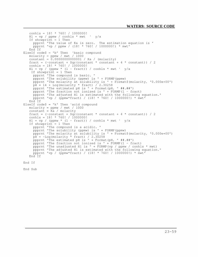
WATER9: SOURCE CODE
23-59
conhls = 18! * 760! / 1000000!Hl = vp / ppmw / conhls * mwt ' y/xIf showprint = 1 Then
ppprnt "The value of Ka is zero. The estimation equation is "ppprnt "vp / ppmw / (18! * 760! / 1000000!) * mwt"
End IfElseIf code$ = "b" Then 'basic compound
molarity = ppmw / mwt / 1000constant = 0.00000000000001 / Ka / (molarity)fract = (-constant + Sqr(constant * constant + 4 * constant)) / 2conhls = 18! * 760! / 1000000!Hl = vp / (ppmw * (1 - fract)) / conhls * mwt ' y/xIf showprint = 1 Thenppprnt "The compound is basic. "ppprnt "The solubility (ppmw) is " + FORMP(ppmw)ppprnt "The molarity at solubility is " + Format$(molarity, "0.000e+00")pH = 14 + Log(molarity * fract) / 2.30258ppprnt "The estimated pH is " + Format(pH, " ##.##")ppprnt "The fraction not ionized is " + FORMP(1 - fract)ppprnt "The adjusted Hl is estimated with the following equation."ppprnt "vp / (ppmw*fract) / (18! * 760! / 1000000!) * mwt"
End IfElseIf code$ = "k" Then 'acid compound
molarity = ppmw / mwt / 1000constant = Ka / molarityfract = (-constant + Sqr(constant * constant + 4 * constant)) / 2conhls = 18! * 760! / 1000000!Hl = vp / (ppmw * (1 - fract)) / conhls * mwt ' y/xIf showprint = 1 Then
ppprnt "The compound is a acidic. "ppprnt "The solubility (ppmw) is " + FORMP(ppmw)ppprnt "The molarity at solubility is " + Format$(molarity, "0.000e+00")pH = -Log(molarity * fract) / 2.30258ppprnt "The estimated pH is " + Format(pH, " ##.##")ppprnt "The fraction not ionized is " + FORMP(1 - fract)ppprnt "The unadjusted Hl is " + FORMP(vp / ppmw / conhls * mwt)ppprnt "The adjusted Hl is estimated with the following equation."ppprnt "vp / (ppmw*fract) / (18! * 760! / 1000000!) * mwt"
End If
End If
End Sub

WATER9: EXAMPLES OF COLLECTION UNIT SPECIFICATIONS
24-1
24. COLLECTION SYSTEM EXAMPLE The following example illustrates the use of the collection system units to specify a complex system. The below figure illustrates a collection system that has a waste flow to be modeled. The waste enters the system through a drain. The waste mixes with the underflow and then passes through reach B under an open drain. The waste mixture continues down reach C and flows into a junction box.
This collection system is modeled in four units:
1. Reach A with no wastewater flow. 2. the initial waste discharge in unit B (drain unit and reach B); 3. open hub C and reach C; and 4. open sump and flow through the junction box (junction box).
waste inlet open hub air in
reach B reach Creach A
waste underflow
open sump, air flow out
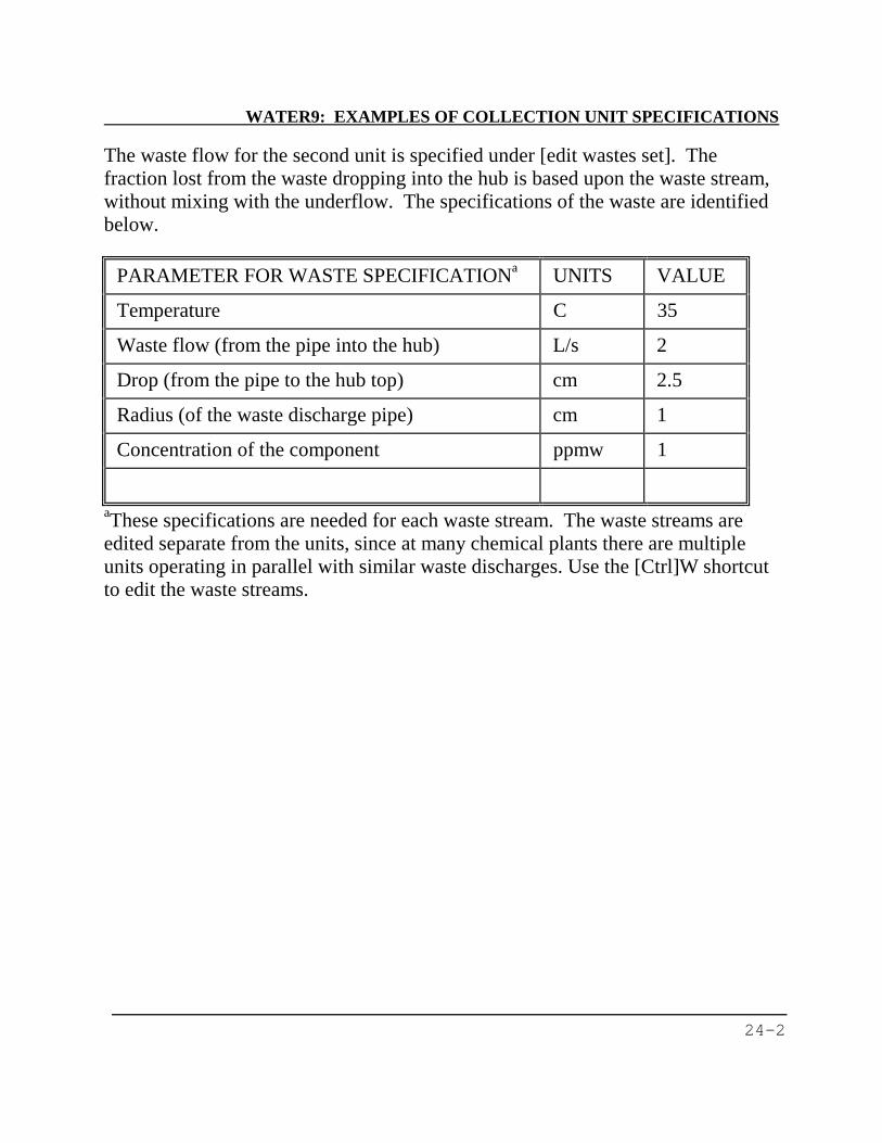
WATER9: EXAMPLES OF COLLECTION UNIT SPECIFICATIONS
24-2
The waste flow for the second unit is specified under [edit wastes set]. The fraction lost from the waste dropping into the hub is based upon the waste stream, without mixing with the underflow. The specifications of the waste are identified below.
PARAMETER FOR WASTE SPECIFICATIONa UNITS VALUE
Temperature C 35
Waste flow (from the pipe into the hub) L/s 2
Drop (from the pipe to the hub top) cm 2.5
Radius (of the waste discharge pipe) cm 1
Concentration of the component ppmw 1
aThese specifications are needed for each waste stream. The waste streams are edited separate from the units, since at many chemical plants there are multiple units operating in parallel with similar waste discharges. Use the [Ctrl]W shortcut to edit the waste streams.
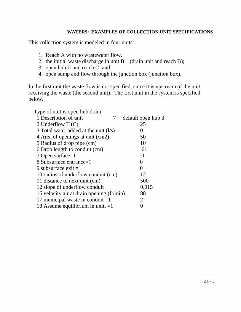
WATER9: EXAMPLES OF COLLECTION UNIT SPECIFICATIONS
24-3
This collection system is modeled in four units:
1. Reach A with no wastewater flow. 2. the initial waste discharge in unit B (drain unit and reach B); 3. open hub C and reach C; and 4. open sump and flow through the junction box (junction box).
In the first unit the waste flow is not specified, since it is upstream of the unit receiving the waste (the second unit). The first unit in the system is specified below. Type of unit is open hub drain 1 Description of unit 7 default open hub d 2 Underflow T (C) 25 3 Total water added at the unit (l/s) 0 4 Area of openings at unit (cm2) 50 5 Radius of drop pipe (cm) 10 6 Drop length to conduit (cm) 61 7 Open surface=1 0 8 Subsurface entrance=1 0 9 subsurface exit =1 0 10 radius of underflow conduit (cm) 12 11 distance to next unit (cm) 500 12 slope of underflow conduit 0.015 16 velocity air at drain opening (ft/min) 88 17 municipal waste in conduit =1 2 18 Assume equilibrium in unit, =1 0

WATER9: EXAMPLES OF COLLECTION UNIT SPECIFICATIONS
24-4
This collection system is modeled in four units:
1. Reach A with no wastewater flow. 2. the initial waste discharge in unit B (drain unit and reach B); 3. open hub C and reach C; and 4. open sump and flow through the junction box (junction box).
In the second unit the waste flow is not specified in the unit specifications, since it is specified previously in the waste specification spreadsheet. The characteristics of the second unit in the system are specified below. Type of unit is open hub drain 1 Description of unit 8 default open hub d 2 Underflow T (C) 25 3 Total water added at the unit (l/s) 0 4 Area of openings at unit (cm2) 50 5 Radius of drop pipe (cm) 10 6 Drop length to conduit (cm) 61 7 Open surface=1 0 8 Subsurface entrance=1 0 9 subsurface exit =1 0 10 radius of underflow conduit (cm) 12 11 distance to next unit (cm) 500 12 slope of underflow conduit 0.015 16 velocity air at drain opening (ft/min) 88 17 municipal waste in conduit =1 2 18 Assume equilibrium in unit, =1 0

WATER9: EXAMPLES OF COLLECTION UNIT SPECIFICATIONS
24-5
This collection system is modeled in four units:
1. Reach A with no wastewater flow. 2. the initial waste discharge in unit B (drain unit and reach B); 3. open hub C and reach C; and 4. open sump and flow through the junction box (junction box).
In the third unit the waste flow is not specified, since the waste flow in this unit is downstream of the unit receiving the waste (the second unit). The third unit in the system is specified below. Type of unit is open hub drain 1 Description of unit 9 default open hub d 2 Underflow T (C) 25 3 Total water added at the unit (l/s) 0 4 Area of openings at unit (cm2) 50 5 Radius of drop pipe (cm) 10 6 Drop length to conduit (cm) 61 7 Open surface=1 0 8 Subsurface entrance=1 0 9 subsurface exit =1 0 10 radius of underflow conduit (cm) 12 11 distance to next unit (cm) 500 12 slope of underflow conduit 0.015 16 velocity air at drain opening (ft/min) 88 17 municipal waste in conduit =1 2 18 Assume equilibrium in unit, =1 0
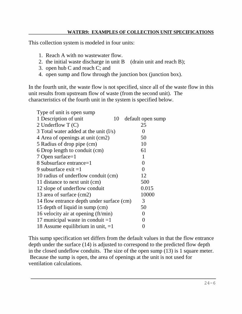
WATER9: EXAMPLES OF COLLECTION UNIT SPECIFICATIONS
24-6
This collection system is modeled in four units:
1. Reach A with no wastewater flow. 2. the initial waste discharge in unit B (drain unit and reach B); 3. open hub C and reach C; and 4. open sump and flow through the junction box (junction box).
In the fourth unit, the waste flow is not specified, since all of the waste flow in this unit results from upstream flow of waste (from the second unit). The characteristics of the fourth unit in the system is specified below. Type of unit is open sump 1 Description of unit 10 default open sump 2 Underflow T (C) 25 3 Total water added at the unit (l/s) 0 4 Area of openings at unit (cm2) 50 5 Radius of drop pipe (cm) 10 6 Drop length to conduit (cm) 61 7 Open surface=1 1 8 Subsurface entrance=1 0 9 subsurface exit =1 0 10 radius of underflow conduit (cm) 12 11 distance to next unit (cm) 500 12 slope of underflow conduit 0.015 13 area of surface (cm2) 10000 14 flow entrance depth under surface (cm) 3 15 depth of liquid in sump (cm) 50 16 velocity air at opening (ft/min) 0 17 municipal waste in conduit =1 0 18 Assume equilibrium in unit, =1 0
This sump specification set differs from the default values in that the flow entrance depth under the surface (14) is adjusted to correspond to the predicted flow depth in the closed undeflow conduits. The size of the open sump (13) is 1 square meter. Because the sump is open, the area of openings at the unit is not used for ventilation calculations.
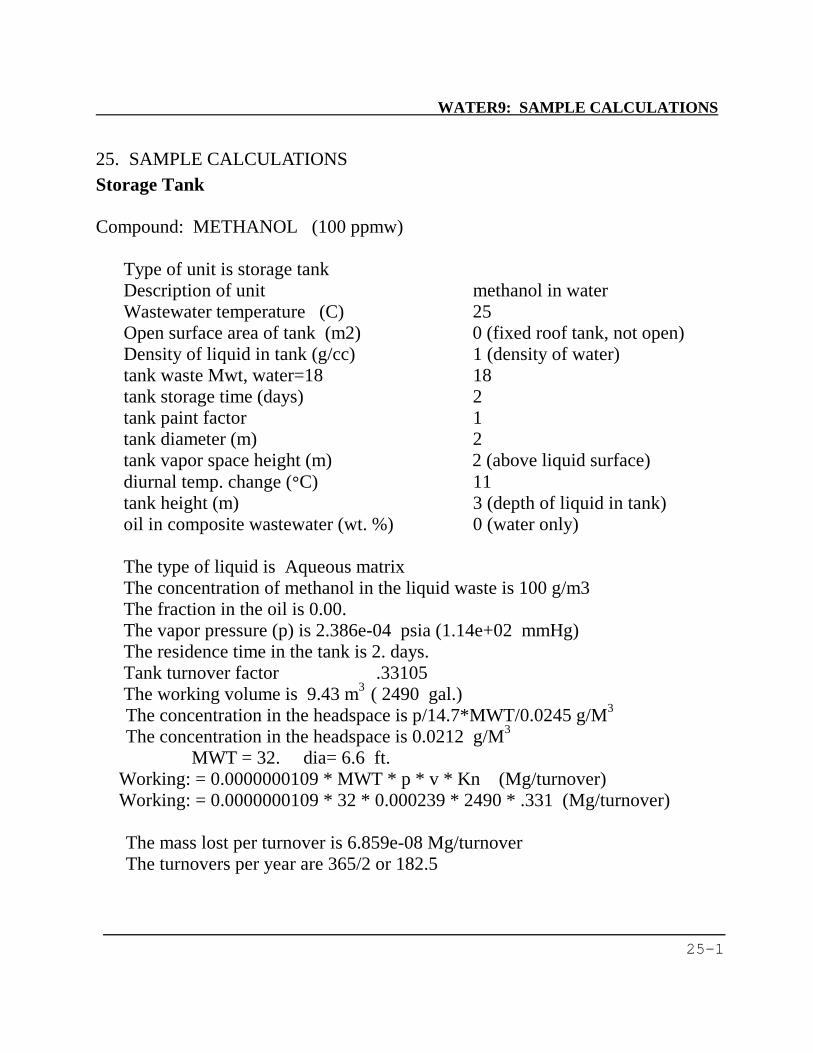
WATER9: SAMPLE CALCULATIONS
25-1
25. SAMPLE CALCULATIONS Storage Tank Compound: METHANOL (100 ppmw) Type of unit is storage tank Description of unit methanol in water Wastewater temperature (C) 25 Open surface area of tank (m2) 0 (fixed roof tank, not open) Density of liquid in tank (g/cc) 1 (density of water) tank waste Mwt, water=18 18 tank storage time (days) 2 tank paint factor 1 tank diameter (m) 2 tank vapor space height (m) 2 (above liquid surface) diurnal temp. change (°C) 11 tank height (m) 3 (depth of liquid in tank) oil in composite wastewater (wt. %) 0 (water only) The type of liquid is Aqueous matrix The concentration of methanol in the liquid waste is 100 g/m3 The fraction in the oil is 0.00. The vapor pressure (p) is 2.386e-04 psia (1.14e+02 mmHg) The residence time in the tank is 2. days. Tank turnover factor .33105 The working volume is 9.43 m3 ( 2490 gal.)
The concentration in the headspace is p/14.7*MWT/0.0245 g/M3
The concentration in the headspace is 0.0212 g/M3
MWT = 32. dia= 6.6 ft. Working: = 0.0000000109 * MWT * p * v * Kn (Mg/turnover) Working: = 0.0000000109 * 32 * 0.000239 * 2490 * .331 (Mg/turnover)
The mass lost per turnover is 6.859e-08 Mg/turnover The turnovers per year are 365/2 or 182.5
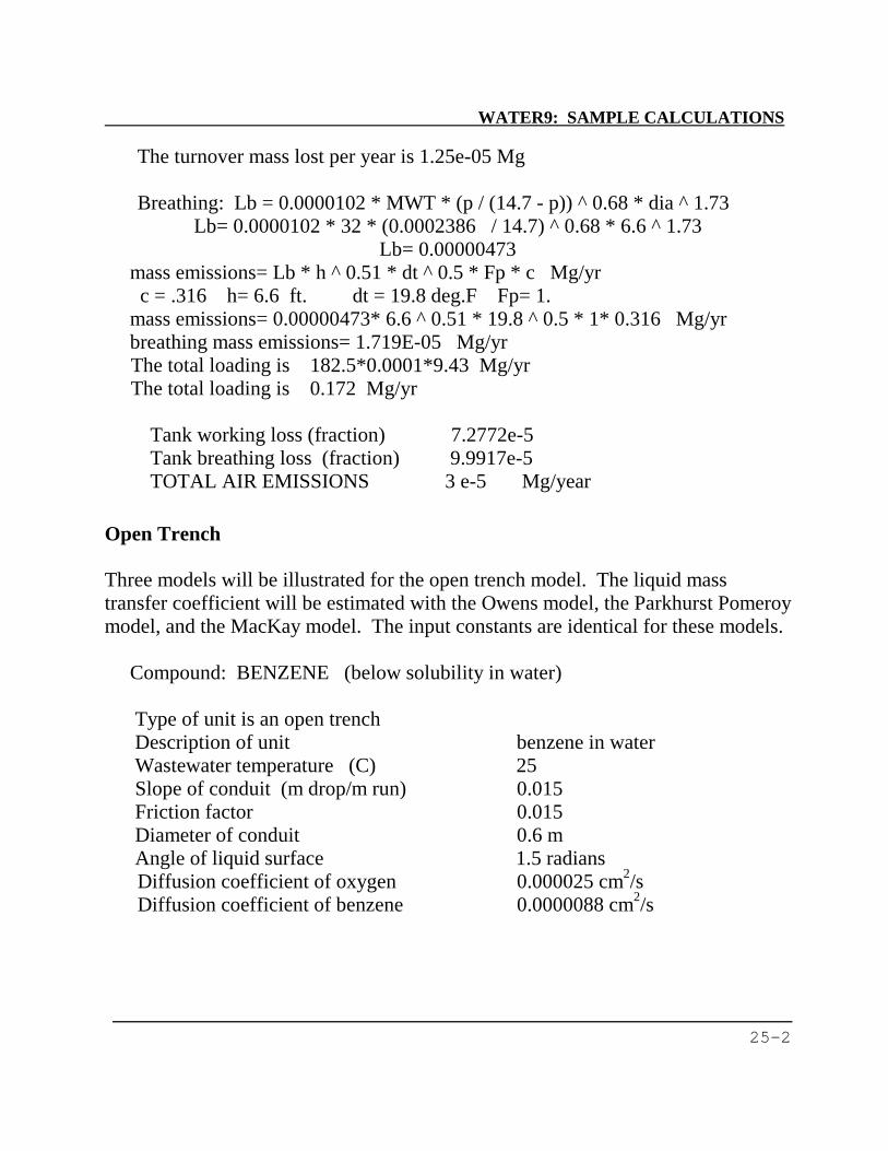
WATER9: SAMPLE CALCULATIONS
25-2
The turnover mass lost per year is 1.25e-05 Mg
Breathing: Lb = 0.0000102 * MWT * (p / (14.7 - p)) ^ 0.68 * dia ^ 1.73 Lb= 0.0000102 * 32 * (0.0002386 / 14.7) ^ 0.68 * 6.6 ^ 1.73
Lb= 0.00000473 mass emissions= Lb * h ^ 0.51 * dt ^ 0.5 * Fp * c Mg/yr c = .316 h= 6.6 ft. dt = 19.8 deg.F Fp= 1. mass emissions= 0.00000473* 6.6 ^ 0.51 * 19.8 ^ 0.5 * 1* 0.316 Mg/yr breathing mass emissions= 1.719E-05 Mg/yr
The total loading is 182.5*0.0001*9.43 Mg/yr The total loading is 0.172 Mg/yr
Tank working loss (fraction) 7.2772e-5 Tank breathing loss (fraction) 9.9917e-5 TOTAL AIR EMISSIONS 3 e-5 Mg/year
Open Trench Three models will be illustrated for the open trench model. The liquid mass transfer coefficient will be estimated with the Owens model, the Parkhurst Pomeroy model, and the MacKay model. The input constants are identical for these models. Compound: BENZENE (below solubility in water) Type of unit is an open trench Description of unit benzene in water Wastewater temperature (C) 25 Slope of conduit (m drop/m run) 0.015 Friction factor 0.015 Diameter of conduit 0.6 m Angle of liquid surface 1.5 radians Diffusion coefficient of oxygen 0.000025 cm2/s Diffusion coefficient of benzene 0.0000088 cm2/s

WATER9: SAMPLE CALCULATIONS
25-3
From these input parameters other input parameters are estimated: Actual depth 0.279 m Hydraulic radius 0.469 m Manning velocity 2.238 m/s Average depth 0.215 m
Owens Model The equation used for the trench model is as follows: Ψ= −− 85.067.051062.7 dUxK L (1) where, KL = liquid mass transfer coefficient for oxygen, m/s, d = depth of flow, ft, U = wastewater mean velocity, ft/s, and Ψ = ratio of mass transfer coefficient to oxygen, (Dvoc/Doxygen).5. Upon substituting values for the input parameters,
( )502.03048.0215.0
3048.0238.21062.7
85.067.05
−−
= xK L (2)
where, KL = liquid mass transfer coefficient for oxygen, 0.000196 m/s, d = depth of flow, .215/.3048 ft, U = wastewater mean velocity, 2.238/.3048 ft/s, and Ψ = ratio of mass transfer coefficient to oxygen, 0.502.
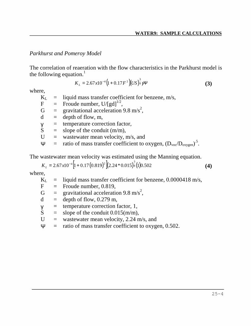
WATER9: SAMPLE CALCULATIONS
25-4
Parkhurst and Pomeroy Model The correlation of reaeration with the flow characteristics in the Parkhurst model is the following equation.1 ( )( ) Ψ+= − γ8
324 17.011067.2 USFxK L (3)
where, KL = liquid mass transfer coefficient for benzene, m/s, F = Froude number, U/[gd]1/2, G = gravitational acceleration 9.8 m/s2, d = depth of flow, m, γ = temperature correction factor, S = slope of the conduit (m/m), U = wastewater mean velocity, m/s, and Ψ = ratio of mass transfer coefficient to oxygen, (Dvoc/Doxygen).5. The wastewater mean velocity was estimated using the Manning equation. ( )[ ]( ) ( ) 502.01015.0*24.2819.017.011067.2 8
324 += −xK L (4) where, KL = liquid mass transfer coefficient for benzene, 0.0000418 m/s, F = Froude number, 0.819, G = gravitational acceleration 9.8 m/s2, d = depth of flow, 0.279 m, γ = temperature correction factor, 1, S = slope of the conduit 0.015(m/m), U = wastewater mean velocity, 2.24 m/s, and Ψ = ratio of mass transfer coefficient to oxygen, 0.502.

WATER9: SAMPLE CALCULATIONS
25-5
Mackay Liquid Mass Transfer Model The MacKay liquid mass transfer model was primarily developed for mass transfer in impoundments.2 The model is based upon shear forces (U*) exerted upon the liquid surfaces by wind flowing overhead. For flow in conduits that is driven by gravity and depends not on wind, but on the slope of the channel bottom, the shear force is estimated from the assumed turbulent profile in the channel. Consider the flow of air over a surface. The wind will generally be turbulent (swirls of wind) even at relatively low air flow rates. As air flows over the surface, there is a drag on the surface induced by the air. This friction or drag can be expressed by the shear at the surface, τ (dynes/cm2). A term that occurs often in the analysis of momentum transfer at surfaces is the friction velocity, U*
U* = (τ gc/ρ)1/2 (5) where: gc is the gravitational constant (980 g-cm/g force - sec2), and ρ is the density (g/cm3). The units of U* are
dynescm
gcmg force
cmg2 2
3
sec
/
1 2
or cm/sec, that has the same units as velocity. Note that at an air water interface, the shear force is the same, but the friction velocity depends on the density of the media. The square root of the density ratios is used to convert a friction velocity from the water friction velocity to the equivalent air friction velocity. Since the correlation of MacKay depends on the friction velocity on the air side, the friction
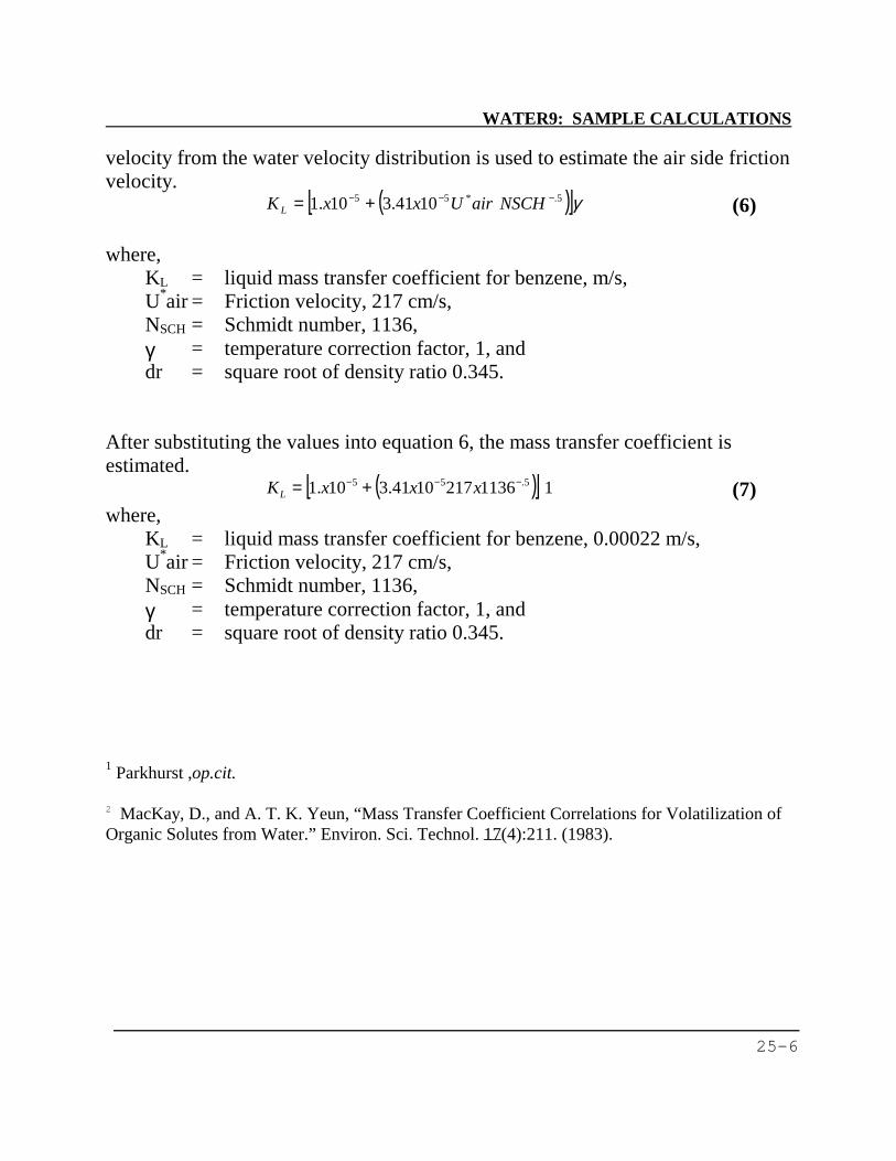
WATER9: SAMPLE CALCULATIONS
25-6
velocity from the water velocity distribution is used to estimate the air side friction velocity. ( )[ ]γ5.*55 1041.310.1 −−− += NSCHairUxxK L (6) where, KL = liquid mass transfer coefficient for benzene, m/s, U*air = Friction velocity, 217 cm/s, NSCH = Schmidt number, 1136, γ = temperature correction factor, 1, and dr = square root of density ratio 0.345. After substituting the values into equation 6, the mass transfer coefficient is estimated. ( )[ ] 111362171041.310.1 5.55 −−− += xxxKL (7) where, KL = liquid mass transfer coefficient for benzene, 0.00022 m/s, U*air = Friction velocity, 217 cm/s, NSCH = Schmidt number, 1136, γ = temperature correction factor, 1, and dr = square root of density ratio 0.345. 1 Parkhurst ,op.cit. 2 MacKay, D., and A. T. K. Yeun, “Mass Transfer Coefficient Correlations for Volatilization of Organic Solutes from Water.” Environ. Sci. Technol. 17(4):211. (1983).

Filename: WATER9 manual.docDirectory: D:\water9work\documentsTemplate: C:\Documents and Settings\cca\Application
Data\Microsoft\Templates\Normal.dotTitle:Subject:Author: Clark AllenKeywords:Comments:Creation Date: 1/17/2001 2:21 PMChange Number: 95Last Saved On: 5/23/2002 9:24 AMLast Saved By: Clark AllenTotal Editing Time: 1,727 MinutesLast Printed On: 5/23/2002 9:27 AMAs of Last Complete Printing
Number of Pages: 188Number of Words: 45,674 (approx.)Number of Characters: 260,342 (approx.)


![Release 2.0.0 Forest Gregg, Derek Eder, and contributors€¦ · dedupe Documentation, Release 2.0.0 • training_file (Optional[TextIO]) – file object containing training data](https://static.fdocuments.in/doc/165x107/5f5c64b05932ce50a9416246/release-200-forest-gregg-derek-eder-and-contributors-dedupe-documentation-release.jpg)