User's Guide for the Rapid Assessmentof the Functional Condition of Stream-

Riparian Ecosystems in the American Southwest

Peter B. Stacey, Allison L. Jones, Jim C. Catlin, Don A. Duff

Lawrence E. Stevens, and Chad Gourley

Table of Contents

Summary . . . . . . . . . . . . . . . . . . . . . . . . . . . . . . . . . . . . . . . . . . . . . . . . . . . . . . . . .2

1. Introduction to the Rapid Stream-Riparian Assessment Method . . . . . . . . . . . .3

Table 1: RSRA indicator variables and justification . . . . . . . . . . . . . . . . . . . . .4

2. Conducting the Rapid Stream-Riparian Assessment . . . . . . . . . . . . . . . . . . . . .8

A. Identify study reach of interest . . . . . . . . . . . . . . . . . . . . . . . . . . . . . . . . . . .8

B. Identify one or more reference reaches . . . . . . . . . . . . . . . . . . . . . . . . . . . . .8

C. Collect background information on the reference reach and study reach . .9

Box 1: Background information to help interpret site visit . . . . . . . . . . . . .9

D. Conduct the RSRA field assessment . . . . . . . . . . . . . . . . . . . . . . . . . . . . . . .11

1. Field Gear . . . . . . . . . . . . . . . . . . . . . . . . . . . . . . . . . . . . . . . . . . . . . . . . . .11

2. Reference Photos . . . . . . . . . . . . . . . . . . . . . . . . . . . . . . . . . . . . . . . . . . . .11

3. Timing . . . . . . . . . . . . . . . . . . . . . . . . . . . . . . . . . . . . . . . . . . . . . . . . . . . . .12

4. Establishment of Transects . . . . . . . . . . . . . . . . . . . . . . . . . . . . . . . . . . . . .12

5. Scoring - General Considerations . . . . . . . . . . . . . . . . . . . . . . . . . . . . . . . .13

6. Tallying the Scores and Interpretation . . . . . . . . . . . . . . . . . . . . . . . . . . . .14

3. Specific Directions for Scoring Each Indicator . . . . . . . . . . . . . . . . . . . . . . . . .14

A. Water Quality . . . . . . . . . . . . . . . . . . . . . . . . . . . . . . . . . . . . . . . . . . . . . . . . .15

B. Hydro-geomorphology . . . . . . . . . . . . . . . . . . . . . . . . . . . . . . . . . . . . . . . . .17

C. Fish/Aquatic Habitat . . . . . . . . . . . . . . . . . . . . . . . . . . . . . . . . . . . . . . . . . . .22

D. Riparian Vegetation . . . . . . . . . . . . . . . . . . . . . . . . . . . . . . . . . . . . . . . . . . . .26

E. Terrestrial Wildlife Habitat . . . . . . . . . . . . . . . . . . . . . . . . . . . . . . . . . . . . . .33

Definitions . . . . . . . . . . . . . . . . . . . . . . . . . . . . . . . . . . . . . . . . . . . . . . . . . . . . . . .35

Appendix 1. Drawings of Aquatic Insect Orders Typically

Found in the Southwestern United States. . . . . . . . . . . . . . . . . . . . .39

Appendix 2. The RSRA Score Sheet . . . . . . . . . . . . . . . . . . . . . . . . . . . . . . . . . . .41

Appendix 3. The RSRA Field Worksheet . . . . . . . . . . . . . . . . . . . . . . . . . . . . . . .47

Appendix 4. Human Impacts Worksheet . . . . . . . . . . . . . . . . . . . . . . . . . . . . . . . .56

1

Revised 28 May 2009

Summary

Stream-riparian ecosystems are among the most productive, biologically diverse and threatened

habitats in arid regions, including the American Southwest. Standardized assessment protocols

are needed in order to effectively measure the current health and functional condition of these

ecosystems, as well as to serve as a guide for future restoration and monitoring programs.

However, most existing survey methods either focus on only a limited subset of the different

components of the ecosystem, base their evaluations upon some hypothesized future state rather

than upon the current conditions of the reach, and/or rely heavily upon subjective judgments of

ecosystem health. We describe an integrated, multi-dimensional method for rapid assessment of

the functional condition of riparian and associated aquatic habitats called Rapid Stream-

Riparian Assessment (RSRA). This method evaluates the extent to which natural processes pre-

dominate in the stream-riparian ecosystem and whether there is sufficient terrestrial and aquatic

habitat complexity to allow for the development of diverse native plant and animal communi-

ties.

The Rapid Stream-Riparian Assessment involves a quantitative evaluation of between two to

seven indicator variables in five different ecological categories: water quality, fluvial geomor-

phology, aquatic and fish habitat, vegetation composition and structure, and terrestrial wildlife

habitat. Each variable is rated on a scale that ranges from "1", representing highly impacted and

non-functional conditions, to "5", representing a healthy and completely functional system.

Whenever possible, scores are scaled against what would be observed in control or reference

sites that have similar ecological and geophysical characteristics, but which have not been heav-

ily impacted by human activities. The protocol was designed to be used both by specialists and

by non-specialists after suitable training. It is particularly appropriate for small to medium sized

streams and rivers in the American Southwest, but with slight modification it also should be

applicable to reaches in other temperate regions and geomorphic settings.

2

1. Introduction to the User’s Guide for the Rapid Assessment of the

Functional Condition of Stream-Riparian Ecosytems in the American

Southwest.

Stream-riparian zones are some of the most productive and important natural resources found

on public and private lands. These ecosystems are highly valued as habitats for fish and

wildlife, as a water source for human communities, for recreation, and for many different eco-

nomic uses. This is particularly true in arid and semi-arid regions like the American Southwest,

where riparian areas support a biotic community whose richness far exceeds the relative total

land area that these systems occupy.

Because of both the ecological importance of riparian areas and their heavy utilization by

humans, there is a need for assessment methods that can be used to objectively evaluate the

existing conditions of the stream-riparian ecosystem, detect at-risk components, prioritize man-

agement strategies and/or possible restoration activities if problems are discovered, and then be

used to objectively monitor any future changes within the system. An effective assessment pro-

tocol must include consideration of the interactions among stream, fluvial wetland, and riparian

habitats (here referred to as the stream-riparian ecosystem), as well as the potential impacts of

upstream and adjacent upland areas.

The Rapid Stream-Riparian Assessment (RSRA) utilizes a primarily qualitative assessment

based on quantitative measurements. It focuses upon five functional components of the stream-

riparian ecosystem that provide important benefits to humans and wildlife, and which, on public

lands, are often the subject of government regulation and standards. These components are: 1)

water quality and pollution, 2) stream channel and floodplain morphology and the ability of the

system to limit erosion and withstand flooding without damage, 3) the presence of habitat for

native fish and other aquatic species, 4) vegetation structure and composition, including the

occurrence and relative dominance of exotic or non-native species, and 5) suitability as habitat

for terrestrial wildlife, including threatened or endangered species.

Within each of these areas, the RSRA evaluates between two and seven variables which reflect

the overall function and health of the stream-riparian ecosystem. The basis for the inclusion of

the individual indicators is briefly summarized in Table 1. A more complete discussion of the

variables, including selected references, can be found in Stevens et al. (2005)1. Definitions of

key terms used in Table 1 are provided at the end of the User's Guide; illustrations of selected

variables accompany the directions for scoring those indicator variables that are included in

Section 3.

3

1 Stevens, L.E., Stacey, P.B., Jones, A. L., Duff, D., Gourley, C., and J.C. Catlin. 2005. A protocol for rapid

assessment of southwestern stream-riparian ecosystems. Proceedings of the Seventh Biennial Conference of

Research on the Colorado Plateau titled The Colorado Plateau II, Biophysical, Socioeconomic, and CulturalResearch. Charles van Riper III and David J. Mattsen, Ed.s pp 397-420. Tuscon, AZ: University of Arizona Press.

Table 1: RSRA indicator variables and the reasons for including them in the protocol.

4

5

Table 1: Continued from the previous page.

Indicator Selection

Four principles guided our selection of the specific variables that are included in the RSRA.

First, we focus on indicators that not only measure the ability of the system to provide specific

functions, but that at the same time reflect other important ecological processes within the

stream-riparian system. For example, in the fish habitat section we consider the relative amount

of undercut banks along the reach. Undercut banks not only provide important habitat and cover

for fish and other aquatic species, but their presence indicates that the bank itself is well vege-

tated, and that there is sufficient root mass to allow the development of the hour-glass shape

channel cross-section typical of most healthy stream systems. This in turn would suggest that

the fluvial processes of erosion and deposition along that stretch of the reach are in relative

equilibrium.

Second, we focus on variables that could be measured rapidly in the field and that would not

require specialized equipment or training. As a result, the protocol can be conducted not only

by specialists, but also by conservationists, agency personnel, ranchers, and interested lay-peo-

ple that have received some initial training. More detailed methods have been developed for

many of the individual indicators included in this protocol. However, because they often require

considerable time and expensive equipment, the use of such protocols will often limit the other

kinds of information that can be reasonably collected from the reach. Our goal was to obtain an

overall picture of the functioning of the system under assessment within a two to three hour

period. Should any of the individual components of the reach be found to be particularly prob-

lematic or non-functional, the more specialized methods can then be used during later visits to

collect additional quantitative information on that variable.

Third, we measure only the current condition of the ecosystem, rather than creating scores that

are based upon some hypothesized future state or successional trend. That is, we are concerned

with the ability of the ecosystem to provide some important function at the present time, and

not whether it would be likely to do so at some point in the future, if current trends or manage-

ment practices continue. We use this approach because stream-riparian systems are highly

dynamic and they are often subject to disturbances (e.g., large flooding) that will alter succes-

sional trends and make predictions of future conditions highly problematic.

In addition, by evaluating only current conditions, this protocol can be used as a powerful tool

for monitoring and measuring future changes in the functional status of the system. For exam-

ple, if a reach is rated as in poor condition with respect to a particular set of parameters, reeval-

uating the system using the identical protocol in subsequent years gives one the ability to meas-

ure the effectiveness of any management change or active restoration program and to undertake

corrections if the restoration actions are found to be not producing the desired changes. This

type of adaptive management approach can be extremely difficult if the evaluation and monitor-

ing measures are based primarily upon the expectations of some future, rather than current, con-

dition.

Fourth, and for similar reasons, we use a quantitative approach to score variables and

measure ecosystem health. Many current assessment systems that are based upon dichotomous

6

categories, such as "functional/non-functional", or "yes/no", can be subjective and difficult to

repeat in the same way from one year to the next, or when conducted by different observers. In

addition, dichotomous scoring systems often are not able to provide sufficient insight into the

ecological processes that may be affecting the ability of the system to provide (or not provide)

desired functions that would indicate whether active restoration efforts might be necessary. We

used a review of existing assessment and monitoring protocols, extensive external peer-review,

and our own individual research experiences to create a five point scale for each variable. The

maximum score (5 points) is given when that component of the system is fully functional and

healthy, and is what would be found in a similar reach that has not been heavily impacted by

humans. The minimum score (1 point) is given when the component is completely non-func-

tional, and when it is not capable of providing the desired ecosystem value of that variable.2

Reference Reaches

Every stream will have its own geologic and watershed characteristics that will necessarily limit

both its potential geomorphic form and its ultimate ecological function. For example, streams in

narrow bed-rock canyons will never develop the same number of meanders and floodplain

width as will similarly sized streams that run through broad alluvial fans. For this reason, we

suggest that whenever possible, the stream reach under evaluation should be compared to a ref-

erence reach, and the scores given be scaled with respect to that reach. Reference areas should

have similar geomorphic, fluvial and biological characteristics to the study reach, and should be

as free as possible of current and past human impacts. When this type of reference reach is not

available, ratings should be based upon what the observer would expect to see if all physical

and ecological processes were occurring without human impact, while allowing for natural dis-

turbance processes that may be characteristic of the system.

Geographic Application

The RSRA protocol presented here was developed specifically in reference to small and medi-

um sized stream reaches in the Colorado Plateau and in the adjacent areas of the American

Southwest. It applies most directly to low and mid-gradient watercourses, and therefore will be

most useful in the lower and middle elevation watersheds of this region. Large streams and

rivers, as well as those at high elevations in mountainous regions that have high gradients, are

often subject to forces and conditions that are not fully considered here and therefore may not

be adequately described by this protocol. With only slight modification, the RSRA should be

applicable to many other parts of the American West, as well as to other arid and semi-arid

regions of the world.

7

2 The range of scores used in the RSRA method from 1 to 5 is similar to the functional condition judgments used

by the US Bureau of Land Management and other agencies in their “Proper Functioning Condition” (PFC) assess-

ment protocol (USDI 1998). In that system, streams are rated as ranging from either “not in proper functioning

condition,” which would be equivalent to mean scores of 1-2 in the RSRA, to “in proper functioning condition,”

which would be equivalent to means scores of 4-5 in the RSRA. Intermediate scores in the RSRA protocol (>2 -

<4) can be considered to be equivalent to the “functional at risk” rating in the PFC protocol. Additional discussion

of the similarities and differences between the RSRA and PFC survey protocols is given in Stevens et al. (2005).

2. Conducting the Rapid Stream-Riparian Assessment

The overall approach for assessing stream-riparian health with the RSRA protocol is to:

A. Identify the specific reach of interest within a watershed

B. Identify, if possible, a reference area for that reach with similar geomorphology and biotic

structure

C. Collect as much background information on the reach as is available and appropriate

D. Conduct the protocol in the field

We recommend that the protocol be conducted by a team of at least two or three people, and

that each team member read this User's Guide and become familiar with the RSRA Field

Worksheet and Score Sheet (Appendices 2 and 3) before beginning the field surveys.

A. Identify the Study Reach of Interest

The segment of a stream or river that is to be examined should be representative of the area of

interest, and it should generally be relatively uniform in character, landform, geology and vege-

tation. The study reach should be approximately 1 km in length, and, when possible, include at

least 3-4 stream meanders. Different reaches within a watershed may have different characteris-

tics due to varying geology, hydrology, elevation, and past histories of land use. In such cases,

it is appropriate to conduct separate evaluations in several different reaches. The location of the

study stream reach should be representative of the range of conditions found in the watershed

and should not be chosen to illustrate particularly good (or bad) conditions that would bias the

scores given to the entire stream.

B. Identify One or More Reference Reaches

Because of the long history of occupation and use by Native Americans and Hispanic and

Anglo settlers, it can often be difficult to visualize the natural or unaltered condition of many

western streams and rivers. Therefore, whenever possible, reference sites should be identified

and visited prior to conducting the protocol on the study reach itself. These sites can also be a

good location to train new individuals about general ecological and fluvial processes, as well as

in the use of the protocol itself.

In choosing a reference reach, the team should look for systems with the following characteris-

tics: 1) similar geology, elevation, and flow patterns (both in the amount and timing of peak and

average water flows) to the study reach; and 2) nearly natural or close to natural conditions and

as free as possible from recent and historic human caused disturbances, especially water diver-

sions, roads, livestock grazing, mining, and ground water pumping. Streams that have been sub-

ject to recent catastrophic disturbances such as fires or heavy flooding will not usually serve as

good reference reaches since they may still be in the process of recovering or reaching a new

equilibrium after the disturbance.

8

In some situations, a good reference site may not be available in the immediate area. In these

cases, streams in other watersheds or regions that have similar geomorphic and ecological fea-

tures can be used to gain a basic understanding of the general fluvial and ecological processes

that would be expected in the study reach under unaltered conditions, and can thus offer a rea-

sonable "surrogate" reference site.

C. Collect Background Information on the Reference Reach and Study Reach

Prior to using RSRA in the field, it is recommended that the user collect some basic, back-

ground information on the study reach (see Box 1 for specific suggestions). In a few cases,

information gathered ahead of time will be needed to complete a score sheet item; those cate-

gories marked optional will be helpful to interpreting the field scores, but are not needed to

assign the actual scores themselves.

9

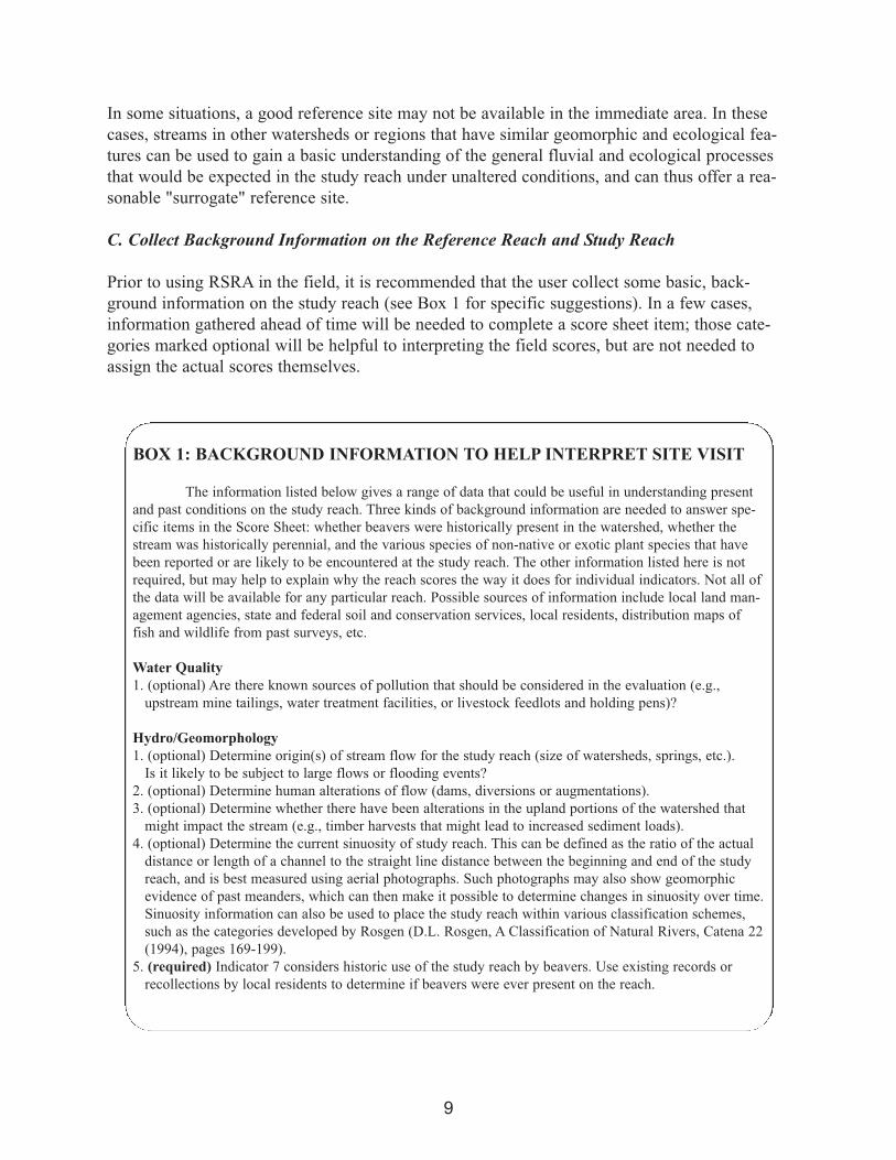
BOX 1: BACKGROUND INFORMATION TO HELP INTERPRET SITE VISIT

The information listed below gives a range of data that could be useful in understanding present

and past conditions on the study reach. Three kinds of background information are needed to answer spe-

cific items in the Score Sheet: whether beavers were historically present in the watershed, whether the

stream was historically perennial, and the various species of non-native or exotic plant species that have

been reported or are likely to be encountered at the study reach. The other information listed here is not

required, but may help to explain why the reach scores the way it does for individual indicators. Not all of

the data will be available for any particular reach. Possible sources of information include local land man-

agement agencies, state and federal soil and conservation services, local residents, distribution maps of

fish and wildlife from past surveys, etc.

Water Quality

1. (optional) Are there known sources of pollution that should be considered in the evaluation (e.g.,

upstream mine tailings, water treatment facilities, or livestock feedlots and holding pens)?

Hydro/Geomorphology

1. (optional) Determine origin(s) of stream flow for the study reach (size of watersheds, springs, etc.).

Is it likely to be subject to large flows or flooding events?

2. (optional) Determine human alterations of flow (dams, diversions or augmentations).

3. (optional) Determine whether there have been alterations in the upland portions of the watershed that

might impact the stream (e.g., timber harvests that might lead to increased sediment loads).

4. (optional) Determine the current sinuosity of study reach. This can be defined as the ratio of the actual

distance or length of a channel to the straight line distance between the beginning and end of the study

reach, and is best measured using aerial photographs. Such photographs may also show geomorphic

evidence of past meanders, which can then make it possible to determine changes in sinuosity over time.

Sinuosity information can also be used to place the study reach within various classification schemes,

such as the categories developed by Rosgen (D.L. Rosgen, A Classification of Natural Rivers, Catena 22

(1994), pages 169-199).

5. (required) Indicator 7 considers historic use of the study reach by beavers. Use existing records or

recollections by local residents to determine if beavers were ever present on the reach.

10

BOX 1: Continued from page 10.

Fish/Aquatic Habitat (F/A)

1. (required) Perennial Flow (F/A qualifier). In order to answer this question, the user needs to know

whether the reach flowed throughout the year in pre-settlement times. Helpful resources include

historical literature and interviews with local residents. Obtain information when available on the

extent of current dewatering and stream regulation, including the frequency at which water is now

completely or partially removed from the stream or spring, or when it is regulated to the point where

little to no water flows during drier times of the year.

2. (optional) Obtain information on the native fishes that potentially could occupy the reach, as well as any

sensitive, indicator, and state or federally listed species. Are there barriers to fish movement (dams,

diversion structures, etc.), either down or upstream from the study reach? Have non-native sport fish

been introduced to the watershed or sub-basin?

3. (optional) Are there presence/absence or relative abundance data for aquatic macroinvertebrates from

past stream surveys?

Riparian Vegetation

1. (required) Indicators 16 and 17 require an understanding of which species are introduced or non-native.

In the American Southwest, salt cedar (tamarisk), Russian olive, Russian thistle, and cheatgrass are often

common non-native and invasive species. However each area may have individual grass, forb or woody

species that are a particular problem. Consult with agency personnel and local residents about such

species, and learn to identify them in advance. Pamphlets are often available from government or private

groups to help identify local exotic problem species.

2. (optional) Gather information on ungulate impacts to the riparian zone from past management studies,

such as forage utilization studies, indications of past problems with grazing, etc.

Wildlife/Habitat (WH)

1. (optional) Obtain a list of current or previously recorded sensitive, indicator, and state or federally listed

species in the reach or in the general area.

Human Activities/Impacts

(optional) Additional data that will be useful to interpret the condition of the reach include information on

historical and current land management practices in the area (including the adjacent uplands), past roads in

the stream bed or riparian area, timber harvests in the watershed, and current recreational and off-highway

vehicle use. The grazing history of the area can also be valuable when available, including livestock

capacity, utilization, season of use, animal numbers permitted in Allotment Management Plans for public

grazing lands, actual and reported use, reports of trespass grazing, efforts to restrict access of livestock to

riparian areas by fencing, etc.

D. Conduct the RSRA field assessment

1. Needed Field Gear

Copies of RSRA Score Sheet (Appendix 2) and Field Worksheets (Appendix 3),

clipboards, pencils, or waterproof pens.

50 or 100 meter tape to measure transects.

Topographic maps of the area, including the watershed upstream from the study

reach (both 1:24,000 and 1:100,000 scales are useful). Aerial photos also can be

helpful.

Camera (digital cameras that automatically record the time and date are best for

taking reference photos.

Flagging to mark the end of transects.

Ocular tube (a "layperson's version" can easily be constructed with an old toilet

tissue cardboard roll or 6” long 2” diameter PVC pipe with "crosshairs" made of thread

across one end).

Global Positioning System (GPS) unit to obtain accurate locations for return visits

to the study reach.

An inexpensive laser level, tripod as small as 6 inches high to hold the level,

and tape measure for measuring historic floodplain to current bankfull ratios.

A straight stick such as adjustable hiking stick (also called trekking pole) is needed.

An adjustable marker such as a velcro strap to mark the location of the laser

light on the vertical stick used in bankfull measurements.

Field guides for plants of the region, including exotic species (optional).

Calculator for determining scores.

Hand lens for identifying stream macroinvertebrates (optional).

2. Reference Photographs

Reference photos can provide an important

visual record of the conditions of the reach

during the survey period. At a minimum,

two reference photos should be taken. The

first should be made at the beginning

(upstream) end of the survey reach, looking

downstream, and the second at the end of

the reach, looking upstream. These two pho-

tos will become part of the permanent sur-

vey record, and can be stored along with the

survey forms in a centralized database.

Additional photos may be taken as appropri-

ate and useful, but are not required. For each

reference photo, the following information

from the score sheet should be added to the

photograph itself:

11

Example: The downstream reference photo of a survey

reach on the Mancos River in Colorado at the top of the

survey stream reach. Note that the necessary information

has been added to the photograph Photo by Peter Stacey.

a) river name and state, stream reach name, date and elevation,

b) which end of the reach is recorded in the photo (upstream or downstream), and

c) UTM coordinates of where the photo was taken.

Using digital cameras and simple photo editing programs, this information can easily be added

to the photograph at a later date, and will provide a permanent label for the photo.

3. Timing

The best time to visit both the reference and study reaches is between late spring and early fall,

when the riparian vegetation is fully developed and when continuous surface water flows are

most critical to wildlife. The best times of day for conducting the survey are from 10:00am to

2:00pm, when the sun is well overhead. Shadows cast over the stream at mid-day are used for

one of the indicators.

4. Establishment of Transects

Data will be collected both from the entire 1 kilometer (six tenths of a mile) study reach and

along several 200 meter sample transects located in the stream channel and on the adjacent

banks. The team should first walk the entire reach together. In addition to getting a general

sense of the area, the users also will be scoring some of the indicators during the initial walk-

through. Look for a good location to establish the 200m transects for detailed measurements of

certain variables. You will collect data from three different but adjacent transects along the

same 200m section of the reach: an in-stream transect and a Riparian Zone transect (see below

for details). The location of the transects should be representative of the range of conditions

found along the study reach. It should not be chosen to illustrate particularly good (or bad) con-

ditions that would thereby bias the scores given the reach.

To set up the transects, first mark the beginning of the in-stream or channel transect with a flag,

measure 200 meters either upstream or downstream, and follow the center of the channel when

making measurements. If there are several channels, follow the main channel in the stream.

Flag the end of the transect (make sure that all flagging and other materials are removed at the

end of the survey). Then, using the same starting point, measure 200m along the edge of the

channel that marks the beginning of the Riparian Zone. This transect will usually be along the

edge of the bankfull level of channel or the edge of the channel if the stream is dry. Make sure

that the bank of the main channel is followed. Do not include islands in the transect. Also, do

not include bridges, dams, reservoirs or other similar structures in the transect or in the entire

study reach if possible. Finally, and again using the same starting point, measure 200m just out-

side (in the direction away from the stream) of banfull that marks the boundary of the Riparian

Zone (the bankfull location, or area that is flooded during peak flows in most years; see Figure

1). Because the channel and the terraces may follow different paths, the ending point of all

three transects may not be located at the same precise place.

All locations (including the start and end points of the study reach, the starting point and direc-

tion [upstream or downstream] of the 200m sample transects, and reach photo reference points)

12

should be located with a GPS unit and recorded on the Score Sheet. Photographs to illustrate

the current conditions at the site should be taken at least at the upstream and downstream ends

of the stream reach, at each end of the 200m stream transect looking downstream and upstream,

as well as any other location that would be valuable for future comparisons. Photographs should

include geologic features and the horizon to make relocation of the photo site easier in the

future.

5. Scoring - General Considerations

The 1-5 point range of scoring values assigned to each indicator on the RSRA Score Sheet

either involves specific values for that indicator, or may use terms such as "few," "slight," "lim-

ited," "moderate," "substantial," or "abundant." In both situations, the evaluation team's experi-

ence in the reference riparian area(s) is very important to establish a standard of geomorphic

consistency and expected values for measurement. A score of "N/A" (Not Applicable) is

assigned to variables that are not applicable to the particular reach being assessed. The Field

Worksheet in Appendix 3 organizes tasks by the initial whole reach walkthrough and the in-

stream and vegetation sample transects. This worksheet will help simplify the observation and

data collection process but may not be necessary for highly experienced observers.

Each indicator is measured and the data recorded in the field, along with any additional com-

ments that would assist in future interpretation of results. The most efficient method of scoring

involves partitioning tasks among the team. For example, one individual who is well-versed in

riparian plants may walk the 200m Upper and Lower Riparian transects, while another team

member who is more familiar with fluvial morphology and aquatic habitats can take measure-

ments along the 200m in-stream transect.

The Overall Comments section at the end of the score sheet should be used to discuss the gen-

eral conditions of the stream, as well as any extreme or unexpected conditions that are observed

during the survey. These comments can be a very useful verbal summary of the most important

findings of the assessment

After the initial data are collected on the worksheets, all members of the team should meet to

discuss their evaluations and scoring assignment for the Assessment Score Sheet, as well as any

recommendations the team may make for the possible future restoration of the reach. It is

important to emphasize that variables are scored entirely on the basis of existing conditions

within the reach and not on any potential or hypothesized future condition.

An additional worksheet on Human Impacts is included as Appendix 4. This worksheet should

be used to take note of various types of human activities and impacts that are occurring on the

study reach or adjacent areas. This information is not used in the scoring because the RSRA

method is specifically designed to measure the current ecological functioning and condition

(health) of the reach, regardless of how those conditions came about. However, it can be useful

to take note of human-related impacts in the stream channel and floodplain, as these may

explain why certain indicators may receive low functional scores. This information may also

provide suggestions for future restoration projects if needed.

13

6. Tallying the Scores and Interpretation

After completing all the field surveys, the observation team should rate each indicator from 1 to

5, using the scoring definitions on the Score Sheet. Then, for each category, calculate and

record the mean score for that set of indicators in that section and on the last page. The overall

score for the surveyed stream reach is then obtained by calculating the overall mean of the five

category mean scores.

An overall mean score of 1-2 indicates that most or all components of the stream are not func-

tioning and that the reach probably cannot provide many of the values of healthy stream-ripari-

an ecosystems. Scores of 2-4 indicate that some components may be in healthy condition while

others are not, and/or that the entire system in general has been impacted by human activities or

natural disturbances in the past, but it is now in a transitional state. The direction of the change,

and whether the system is improving or getting worse, can only be determined by subsequent

visits and monitoring programs. Scores of 4-5 indicate that the ecosystem is healthy and that it

matches what would be expected in a geomorphically similar reference reach or in an unim-

pacted "presettlement" condition. Because of the dynamic nature of stream-riparian ecosystems,

it is very unlikely that any reach, even one in pristine condition, would obtain a mean score of 5

for any category or overall, and this should not be expected.

While a single composite site score is desirable for judging site health and developing regional

restoration priorities as appropriate, such scores should not constitute the final interpretation of

site status. While the overall score may indicate that a stream reach is functioning well, one or

more individual indicators may be extremely off balance. Very low individual or clustered

scores in an otherwise high scoring system often indicate that there are specific impacts on the

stream or riparian area that should be addressed, and which, if not reversed, may eventually

lead to an overall decline in the health of the system. For example, a reach may be functioning

well physically, but be biologically degraded, in which case the need for restoration action

depends on the management goals for that reach, and whether biological functions are impor-

tant. Alternatively, a reach's hydrology and streamflow patterns may be highly altered but the

system might appear otherwise healthy. Thus the interpretation of reach conditions should

involve an analysis of the overall scores against the mean category scores and reference condi-

tions to improve understanding of ecological function and management goals for the reach.

3. Specific Directions for Scoring Each Indicator

The next pages in this next section provide detailed instructions for collecting the information

needed to score each variable. The instructions are given in the order the variables appear on

the Score Sheet. The Field Worksheet organizes the variables according to the physical areas of

observations, resulting in a different order.

14

15

Photo 1: Algal Growth

(Indicator 1). Strands of

filamentous algae in a

reach of the Santa Fe

River below Santa Fe,

New Mexico. The

extensive growth of

algae in this reach is due

to nutrient loading from

upstream sources of pol-

lution. If the entire tran-

sect resembles this

photo, it would receive

a score of 1. Photo byPeter Stacey.

Photo 2: Algal Growth

(Indicator 1). A large

rock about 3 inches

below the water surface

in Calf Creek, Utah.

Much of the surface of

the rock is covered by

single-celled algae. This

type of algal growth is

typical in many undis-

turbed streams in the

American Southwest,

and should not be count-

ed while measuring

Indicator 1. If the entire

transect appears as

shown in this photo, it

would receive a score of

5. Photo by PeterStacey.

A. Water Quality

Indicator 1. Algal Growth.

Starting at the downsteam end of the 200m in-stream transect, walk in the channel about 1 m.

from the water's edge and, using the ocular tube, every 2 meters record the presence or absence

of filamentous algae. If the reach is <2m wide, walk up the middle of the channel. Do not count

the single cell algae that may cover the surface of rocks. Calculate the total percent cover of fil-

amentous algae by dividing number of positive hits by 100. See examples in Photo 1 and 2.

16

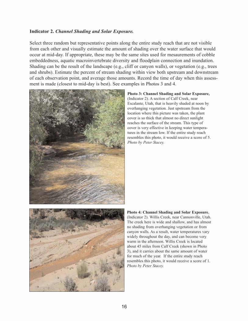
Indicator 2. Channel Shading and Solar Exposure.

Select three random but representative points along the entire study reach that are not visible

from each other and visually estimate the amount of shading over the water surface that would

occur at mid-day. If appropriate, these may be the same sites used for mesaurements of cobble

embeddedness, aquatic macroinvertebrate diversity and floodplain connection and inundation.

Shading can be the result of the landscape (e.g., cliff or canyon walls), or vegetation (e.g., trees

and shrubs). Estimate the percent of stream shading within view both upstream and downstream

of each observation point, and average those amounts. Record the time of day when this assess-

ment is made (closest to mid-day is best). See examples in Photos 3 and 4.

Photo 3: Channel Shading and Solar Exposure,

(Indicator 2). A section of Calf Creek, near

Escalante, Utah, that is heavily shaded at noon by

overhanging vegetation. Just upstream from the

location where this picture was taken, the plant

cover is so thick that almost no direct sunlight

reaches the surface of the stream. This type of

cover is very effective in keeping water tempera-

tures in the stream low. If the entire study reach

resembles this photo, it would receive a score of 5.

Photo by Peter Stacey.

Photo 4: Channel Shading and Solar Exposure,

(Indicator 2). Willis Creek, near Cannonville, Utah.

The creek here is wide and shallow, and has almost

no shading from overhanging vegetation or from

canyon walls. As a result, water temperatures vary

widely throughout the day, and can become very

warm in the afternoon. Willis Creek is located

about 45 miles from Calf Creek (shown in Photo

3), and it carries about the same amount of water

for much of the year. If the entire study reach

resembles this photo, it would receive a score of 1.

Photo by Peter Stacey.

17

B. Hydrogeomorphology

Indicator 3. Floodplain Connection and Inundation.

The likelihood that the stream will be able to escape its bank and flow over the floodplain dur-

ing typical high flow events can be measured by the ratio of the height between the channel

bottom and the historic terrace (prior to entrechment that indicates the boundary of the historic

floodplain itself) and the distance between the channel bottom and its first bank (current bank-

full location; see Figures 1 and 2).

To calculate the historic floodplain to current bankfull ratio, choose three random but represen-

tative points along the entire study reach. Use a laser level (or a survey instrument if available)

to measure the distance between the bottom of the channel and current bankfull level (in the

example in Figure 2, this would be 1.2 feet). Then measure the distance or height of the begin-

ning or closest part of the historic floodplain to the channel bottom (1.8 feet in this example).

Next, divide the historic floodplain depth by current bankfull depth. For Figure 2, 1.8 divided

by 1.2 gives 1.5. Use the scoring scale in Figure 3 to determine the score to put on the Score

Sheet for this location. In this example, the observed ratio of 1.5 leads to a score of 2. Repeat

these measurements at two additional representative locations along the reach, and then take the

average of the three ratios to calculate the final score for this indicator. The final score indicates

the level of connectivity between the stream and its floodplain; a high ratio (and low indicator

score) shows less potential for overbank flooding.

Figure 1: Idealized cross section of a small to medium-sized slightly downcut stream and its associated floodplains

in the American Southwest. The areas of the floodplain that are outside of the scour zone are flooded only during

increasingly rarer and increasingly higher flow events. In entrenched streams, the 2nd terrace represents the pre-

entrenched flooplain. The edge of this 2nd terrace close to the stream channel marks the inside edge of the ripari-

an zone as used in this protocol. Illustration by Heidi Snell

Floodplain

Riparian Zone

2nd Terrace

1st Terrace

Uplands

Channel

Bankfull

The easiest way to make these measurements is to first place the laser level on a rock on the

stream bank. Make sure it is level. Place the walking stick at the deepest part of the channel and

shine the laser light on the stick. Mark where the light hits the stick (A). Next move to the cur-

rent bankfull location and

again mark where the

light hits the stick (B).

Finally mark the stick

when placed at the edge

of the historic floodplain

terrace (C). The distance

between A and B is the

bankful height while the

distance between A and C

is the historic floodplain

height.

18

Figure 2: Method used to measure the

ratio between the height above the bot-

tom of the channel to the historic (pre

entrenched) terrace on the floodplain and

the height of the current bankfull level.

This is used for Indicator 3- floodplain

connection and inundation. Illustrationby Heidi Snell

Figure 3: historic floodplain/ cur-

rent bankfull scoring scale. This

scale translates the ratio of the his-

toric floodplain height above the

stream bottom divided by the height

of the current bankfull into an indi-

cator score.

19

Indicator 4. Vertical Bank Stability.

Within the 200m in-stream transect, estimate the length of the channel bank where there are

actively-eroding, near-vertical cut banks. The monitoring method requires collecting the meters

of bank on both sides of the transect that are stable and unstable. In fine soils, the "sloughing

off" of the banks into the channel and deposition of sediments into the stream will be obvious.

Include both sides of the stream. Estimate the total amount of vertical cut banks on each side of

the 200m in-stream transect, and divide by 400m to arrive at the percent cut banks. If the total

distance of both banks with vertical banks is 80m, the percent of cut banks would be 20% (80m

divided by 400m total). See examples in Photos 5 and 6.

Photo 5: Vertical Bank Stability (Indicator 4). A

section of the Sevier River near Hatch, Utah.

Almost all of the eastern bank of the river is bare

soil and shows evidence of vertical instability,

including long sections that have recently col-

lapsed into the stream. If the entire in-stream tran-

sect resembled conditions shown in the photo, it

would receive a score of 1. Photo by Peter Stacey.

Photo 6: Vertical Bank Stability

(Indicator 4). An example where the bank

is actively "sloughing off" along the Rio

Cebolla in the Jemez Mountains, New

Mexico. This reach was being heavily uti-

lized by cattle at the time the photograph

was taken. Photo by Carrell Foxx.

20

Figure 4: Examples of reaches with different levels of hydraulic habitat diversity (Indicator 5). Note that the

number of different hydraulic habitats tends to increase with the number of meanders. Illustration by ChadGourley.

ew = edge water lp = lateral pool

lvr = low velocity run hvr = high velocity run

lgr = low gradient riffle hgr = high gradient riffle

sp = scour pool

Indicator 5. Hydraulic Habitat Diversity.

Count the number of distinctive hydraulic channel features that would provide unique habitats

that are observed in the overall reach walk-through. Look for riffles, scour pools, cobble or

boulder debris fans, flowing side channels, backwaters, sand-floored runs, or other features that

can provide different habitats for fish and other aquatic organisms. Figure 4 gives an example

of reaches with different levels of hydraulic feature diversity.

21

Indicator 6. Riparian Area Soil Integrity.

During the overall reach walkthrough estimate the extent of soil disturbance in the riparian zone

throughout the entire reach. Include both geomorphically inconsistent erosion from human

activities (e.g., roads, trails) as well as damage from livestock and from native ungulates such

as deer and elk. See examples in Photos 7 and 8.

Photo 7: Riparian Area

Soil Integrity (Indicator

6). Photo of riparian area

soil disturbed by off-road

vehicles. Photo by LizThomas.

Photo 8: Riparian Area Soil Integrity

(Indicator 6). A section of the riparian

area of the Rio Cebolla in the Jemez

Mountains, New Mexico, where the soil

has been extensively disturbed by ungu-

late activity. Note the "cow pie" at the

bottom center of the photograph.

Whenever possible, the source of any soil

disturbance found in the reach should be

noted. Photo by Carrell Fox.

22

Indicator 7. Beaver Activity.

Determine during the overall reach walkthrough the extent in the reach of recent beaver activity

within the last year, as indicated by tracks, drags, digging marks, cut stems, burrows, dams, and

caches. If beavers are no longer present but were historically, then score this indicator as 1.

Certain streams don’t allow beavers to construct a dam because of geomorphic factors. This

also should be considered when assessing evidence of beaver activity. If it is known for certain

that beaver were never in the reach, then score this “NA.”

C. Fish/Aquatic Habitat

When assessing the Fish/Aquatic habitat components of the reach, the observer should walk the

entire study reach, and then examine the channel and both banks of the in-stream 200m tran-

sect.

Qualifier: If there is no flow currently, but this reach historically supported a fishery, then the

entire Fish/Aquatic habitat section receives a score of 1. See Box 1 for more information about

this. Once you have determined how the qualifier applies, continue on to the next section.

Indicator 8. Riffle-Pool Systems: Number and Distribution.

In a stream that is in dynamic equilibrium, stretches of fast moving and relatively shallow water

with obvious bubbles (riffles) will usually alternate with sections that are deeper and slower

moving (pools; see Figure 4). Fish use pools to hide and rest, and riffles to lay their eggs. Note

and record the number of pools and riffles within the 200m stream transect. For the purpose of

this indicator, riffles need to have a cobble bottom. Look for geomorphic consistency. For

example, a larger number of pools and riffles will occur per unit distance in medium gradient

streams, while fewer will be typical of high and low gradient streams.

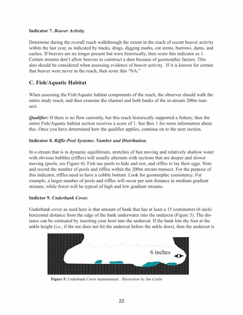
Indictor 9. Underbank Cover.

Underbank cover as used here is that amount of bank that has at least a 15 centimeters (6 inch)

horizontal distance from the edge of the bank underwater into the undercut (Figure 5). The dis-

tance can be estimated by inserting your boot into the undercut. If the bank hits the foot at the

ankle height (i.e., if the toe does not hit the undercut before the ankle does), then the undercut is

6 inches

Figure 5: Underbank Cover measurement. Illustration by Jim Catlin

23

at least 6 inches, and should be counted. Estimate the total amount of underbank cover (under-

cut) along each bank of the 200m in-stream transect, and divide by 400m to arrive at the per-

cent undercover bank. If the total distance of both banks with undercut is 80m, the percent

underbank cover would be 20% (80m divided by 400m total).

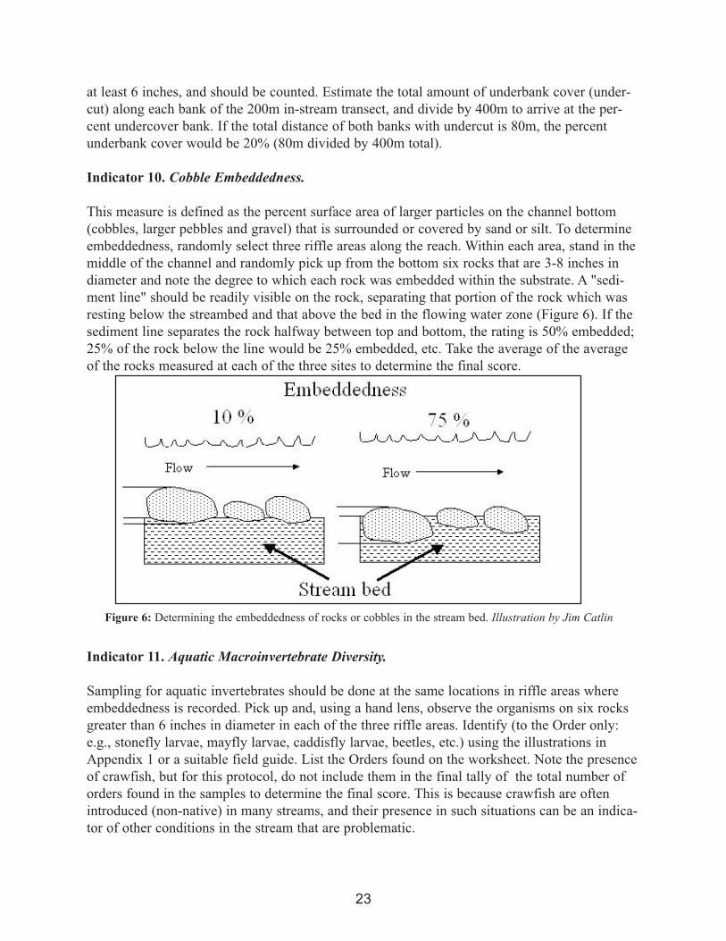
Indicator 10. Cobble Embeddedness.

This measure is defined as the percent surface area of larger particles on the channel bottom

(cobbles, larger pebbles and gravel) that is surrounded or covered by sand or silt. To determine

embeddedness, randomly select three riffle areas along the reach. Within each area, stand in the

middle of the channel and randomly pick up from the bottom six rocks that are 3-8 inches in

diameter and note the degree to which each rock was embedded within the substrate. A "sedi-

ment line" should be readily visible on the rock, separating that portion of the rock which was

resting below the streambed and that above the bed in the flowing water zone (Figure 6). If the

sediment line separates the rock halfway between top and bottom, the rating is 50% embedded;

25% of the rock below the line would be 25% embedded, etc. Take the average of the average

of the rocks measured at each of the three sites to determine the final score.

Indicator 11. Aquatic Macroinvertebrate Diversity.

Sampling for aquatic invertebrates should be done at the same locations in riffle areas where

embeddedness is recorded. Pick up and, using a hand lens, observe the organisms on six rocks

greater than 6 inches in diameter in each of the three riffle areas. Identify (to the Order only:

e.g., stonefly larvae, mayfly larvae, caddisfly larvae, beetles, etc.) using the illustrations in

Appendix 1 or a suitable field guide. List the Orders found on the worksheet. Note the presence

of crawfish, but for this protocol, do not include them in the final tally of the total number of

orders found in the samples to determine the final score. This is because crawfish are often

introduced (non-native) in many streams, and their presence in such situations can be an indica-

tor of other conditions in the stream that are problematic.

Figure 6: Determining the embeddedness of rocks or cobbles in the stream bed. Illustration by Jim Catlin

24

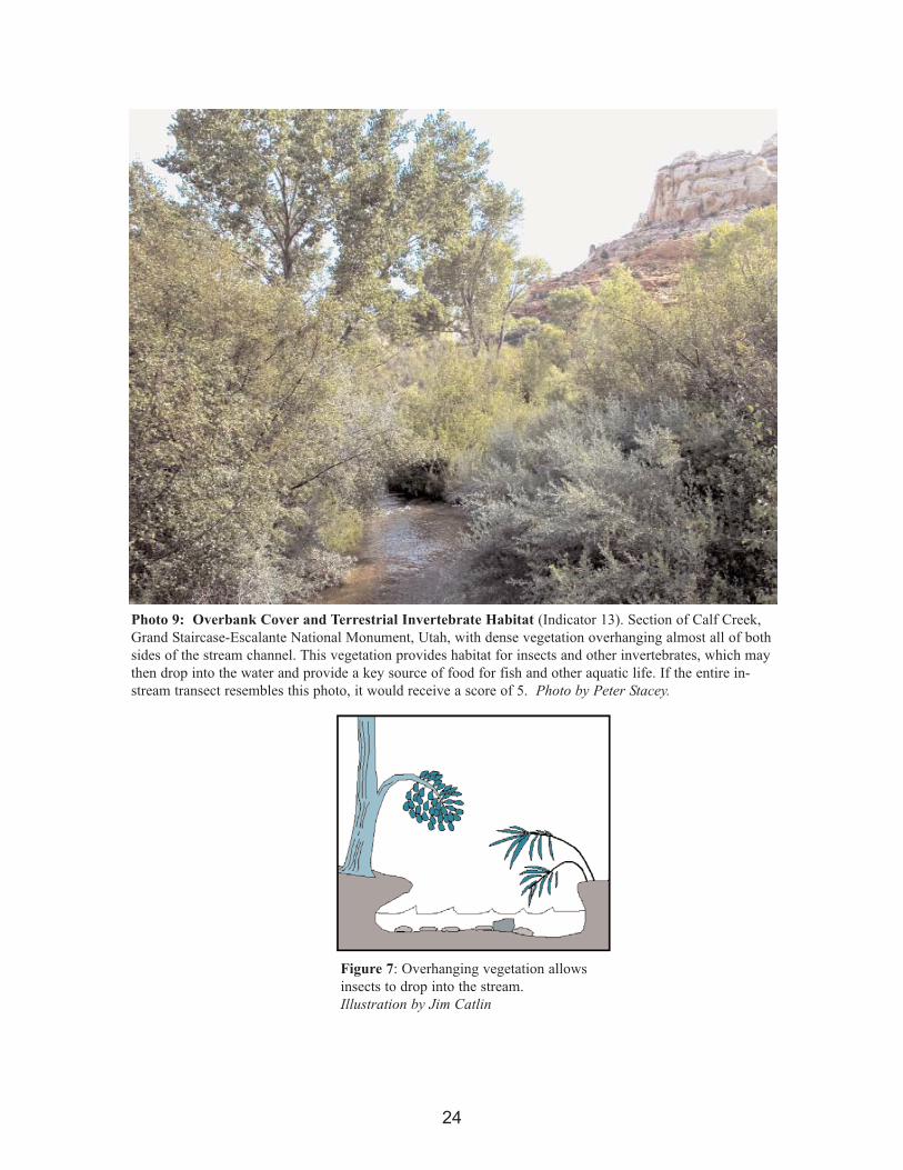
Photo 9: Overbank Cover and Terrestrial Invertebrate Habitat (Indicator 13). Section of Calf Creek,

Grand Staircase-Escalante National Monument, Utah, with dense vegetation overhanging almost all of both

sides of the stream channel. This vegetation provides habitat for insects and other invertebrates, which may

then drop into the water and provide a key source of food for fish and other aquatic life. If the entire in-

stream transect resembles this photo, it would receive a score of 5. Photo by Peter Stacey.

Figure 7: Overhanging vegetation allows

insects to drop into the stream.

Illustration by Jim Catlin

Indicator 12. Large Woody Debris.

This is defined as wood that is not rooted and at least partially in the water or located in the

active stream channel and that is at least 15cm (approximately 6 inches) in diameter and 1m

(approximately 3 feet) in length. Record the number of large woody debris pieces observed

within the 200m in-stream transects.

Indicator 13. Overbank Cover and Terrestrial Invertebrate Habitat.

Insects that drop into the stream from overhanging vegetation (Figure 7; Photos 9 and 10) are a

key source of food and nutrients for fish and other aquatic life. Visually estimate the distance

along both banks of the 200m in-stream transect where there is vegetation (including forbs,

grass, shrubs and trees) hanging over the channel. Use the same technique for calculating this

measurement as is used in indicators 4 and 9.

25

Photo 10: Overbank Cover and Terrestrial Invertebrate Habitat (Indicator 13). In this section of the

Paria River northwest of Page, Arizona, there is little vegetation overhanging the banks of the stream

channel, and therefore little opportunity for insects to drop into the water column. If the entire in-stream

transect resembles this photo, it would score 2. Photo by Peter Stacey.

26

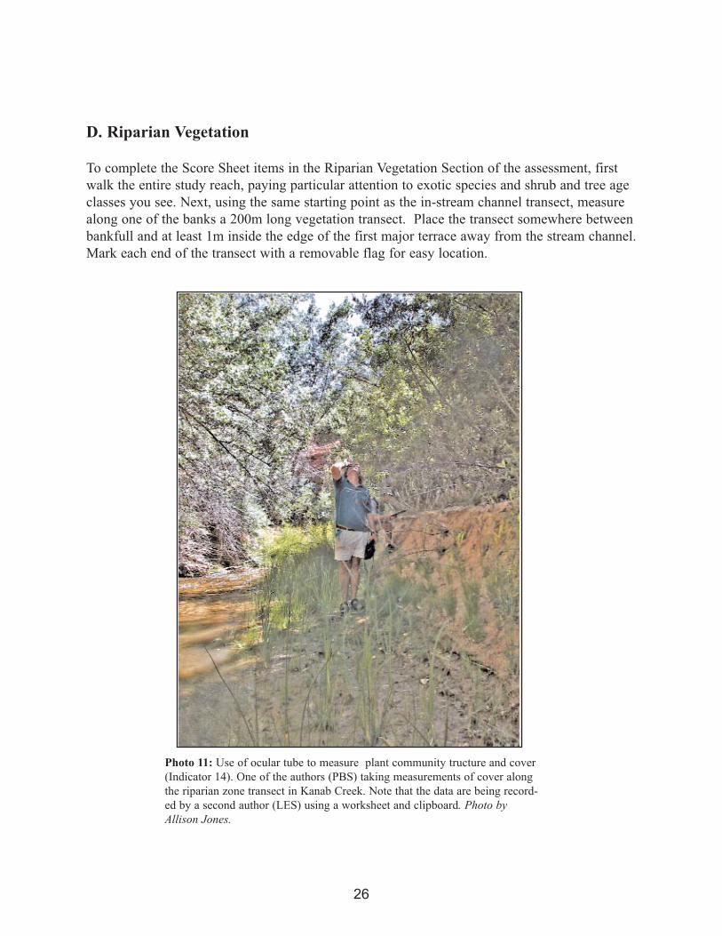
D. Riparian Vegetation

To complete the Score Sheet items in the Riparian Vegetation Section of the assessment, first

walk the entire study reach, paying particular attention to exotic species and shrub and tree age

classes you see. Next, using the same starting point as the in-stream channel transect, measure

along one of the banks a 200m long vegetation transect. Place the transect somewhere between

bankfull and at least 1m inside the edge of the first major terrace away from the stream channel.

Mark each end of the transect with a removable flag for easy location.

Photo 11: Use of ocular tube to measure plant community tructure and cover

(Indicator 14). One of the authors (PBS) taking measurements of cover along

the riparian zone transect in Kanab Creek. Note that the data are being record-

ed by a second author (LES) using a worksheet and clipboard. Photo byAllison Jones.

27

Indicator 14. Riparian Zone Plant Community Structure and Cover.

The presence or absence of vegetation cover observed in each of the four structural layers

(ground, shrub, middle canopy, and upper canopy; see Figure 8) should be recorded for the

riparian transect. In this survey method, Ground layer is a vertical zone that includes both living

grass other herbaceous vegetation, woody plants, and dead vegetative matter up to 1 meter

above the ground. Shrub cover is woody perennial vegetation occurring from 1 meter up to 4

meters above the ground. Middle canopy vegetation is large shrub and small tree cover 4-10

meters above the ground. Upper canopy vegetation is tree cover greater than 10 meters above

the ground. The same species (e.g., cottonwoods) may have individuals in different structural

layers (shrub, middle or

upper canopy), depending

on the particular age of the

plant. Also, noe individual

(i.e. the same cottonwood

tree) can generate “hits” in

multiple canopy categories.

Using an ocular cross-hair

tube and the Field

Worksheet, walk along the

transect and every 2 meters

look directly up and down

through the tube, and

record the presence or

absence of plant material

(dead or alive) intersecting

the vertical sight line of the

cross-hairs in each structur-

al layer - ground cover

layer, shrub layer, mid-

canopy layer and upper

canopy layer (Figure 8 and

Photo 11). The line-of-sight

through the ocular tube

should mimic whether or

not a ray of light originat-

ing directly overhead will

strike any vegetation as it

passes through each layer.

If the line-of-sight falls

upon a rock, score “N/A” (not applicable) for the ground ocver layer, since a plant cannot grow

there. Use the number of "hits" through the ocular tube for cover in each layer (out of 100 sam-

Figure 8: Method of using ocular tube to measure cover in each of the four

structural layers used in Indicator 14. The four hits in the mid canopy

layer are scored as a single “yes” on the worksheet. In this illustration,

there is one hit for upper canopy, four for mid canopy and one hit each in

the shrub and ground layers. Illustration by Heidi Snell.

ples along the 200m transect) to determine percent cover for that layer. Average the percent

cover for the four layers to achieve an overall score. Because local geomorphology can influ-

ence the degree of vegetation cover, the scores from the study reach can be compared with the

average values obtained from an appropriate nearby reference site to help guide interpretation.

Indicator 15 and 16. Native Shrub and Tree Demography and Recruitment.

The distribution of age classes (seedlings, saplings or immature, mature, and snags; see Figure

9 and Photo 12) of the dominant riparian native species in the riparian zone should be deter-

mined during the initial study reach walk-through. As used here, the dominant species is the

one that provides the most vegetative cover throughout the flood plain, and not necessarily the

one that has the most individuals. The observer also should comment on unexpected demo-

graphic conditions, such as the absence of particular age classes of expected dominant species,

such as willows and cottonwoods in the American Southwest.

28

Figure 9: Age classes of shrubs and trees used for Indicators 16 and 17. Cottonwoods (Populus spp) and

willows (Salix spp.) are typical dominant native tree and shrub species in the American Southwest. Other

taxa may be the expected dominant species in other regions or in special situations. Illustration by HeidiSnell.

29

Photo 12: Non-native Herbaceous Plant Species Cover (Indicator 17). Willis Creek, near Cannonville, Utah. The

herbaceous cover in the riparian zone in this part of the reach is composed almost entirely of the exotic Russian

thistle (Salsola kali), with few individuals of native species present. If the study reach resembled this photo, it

would receive a score of 1 for Indicator 17.

Native Tree Demography and Recruitment (Indicator 16). Note that the woody plant cover in the picture is

entirely native, and consists of seedlings and mature cottonwoods. If the entire study reach resembles this photo, it

would score 3 for Indicator 16 because only two age classes for the dominant native tree species are present.

Mammal Browsing on Shrubs and Small Trees (Indicator 20). This section of the stream is heavily utilized by

ungulates. Note the extensive browsing on the cottonwood seedlings as indicated by their heavily branched growth.

See a closeup of the browsed sapling in Photo 14. Contrast this with the unbrowsed cottonwood saplings seen in

photo 16. Photo by Peter Stacey.

30

Indicators 17 and 18. Non-native Herbaceous and Woody Plant Species Cover.

During the initial study reach walkthrough, visually estimate the percentage of cover provided

by non-native shrub, tree, and herbaceous plant species relative to that provided by native

species. Use the background information on exotic or non-native plants to help identify non-

native plants. The cover by a plant is represented by all of the ground area that would be shaded

by that plant if the sun were directly overhead. Include both the flood plain and the riparian

zone for this estimate. Do not consider bare ground and litter cover when making this estimate.

See the examples in Photo 12 and 13.

Photo 13: Non-native Woody Plant Species (Indicator 18). The Fremont River near Cainville, Utah. The south

floodplain of the river is covered almost entirely by non-native shrubs and small trees, primarily salt cedar

(Tamarix ramosissima) and Russian olive (Elaeagnus angustifolia). A few individuals of the native coyote willow

(Salix exigua) can be seen just to the left of the bottom center of the photograph. If the study reach resembles this

photo, it would receive a score of 1 for Indicator 18, non-native woody plant species. Photo by Peter Stacey.

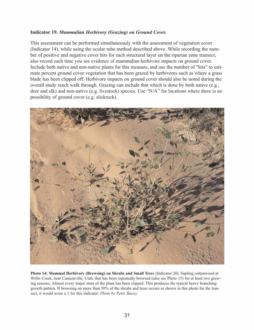
Indicator 19. Mammalian Herbivory (Grazing) on Ground Cover.

This assessment can be performed simultaneously with the assessment of vegetation cover

(Indicator 14), while using the ocular tube method described above. While recording the num-

ber of positive and negative cover hits for each structural layer on the riparian zone transect,

also record each time you see evidence of mammalian herbivore impacts on ground cover.

Include both native and non-native plants for this measure, and use the number of "hits" to esti-

mate percent ground cover vegetation that has been grazed by herbivores such as where a grass

blade has been clipped off. Herbivore impacts on ground cover should also be noted during the

overall study reach walk through. Grazing can include that which is done by both native (e.g.,

deer and elk) and non-native (e.g. livestock) species. Use “N/A” for locations where there is no

possibility of ground cover (e.g. slickrock).

31

Photo 14: Mammal Herbivory (Browsing) on Shrubs and Small Trees (Indicator 20). Sapling cottonwood at

Willis Creek, near Cannonville, Utah, that has been repeatedly browsed (also see Photo 15) for at least two grow-

ing seasons. Almost every major stem of the plant has been clipped. This produces the typical heavy branching

growth pattern. If browsing on more than 50% of the shrubs and trees occurs as shown in this photo for the tran-

sect, it would score a 1 for this indicator. Photo by Peter Stacey.

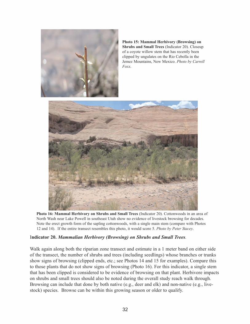
Indicator 20. Mammalian Herbivory (Browsing) on Shrubs and Small Trees.

Walk again along both the riparian zone transect and estimate in a 1 meter band on either side

of the transect, the number of shrubs and trees (including seedlings) whose branches or trunks

show signs of browsing (clipped ends, etc.; see Photos 14 and 15 for examples). Compare this

to those plants that do not show signs of browsing (Photo 16). For this indicator, a single stem

that has been clipped is considered to be evidence of browsing on that plant. Herbivore impacts

on shrubs and small trees should also be noted during the overall study reach walk through.

Browsing can include that done by both native (e.g., deer and elk) and non-native (e.g., live-

stock) species. Browse can be within this growing season or older to qualify.

32

Photo 15: Mammal Herbivory (Browsing) on

Shrubs and Small Trees (Indicator 20). Closeup

of a coyote willow stem that has recently been

clipped by ungulates on the Rio Cebolla in the

Jemez Mountains, New Mexico. Photo by CarrellFoxx.

Photo 16: Mammal Herbivory on Shrubs and Small Trees (Indicator 20). Cottonwoods in an area of

North Wash near Lake Powell in southeast Utah show no evidence of livestock browsing for decades.

Note the erect growth form of the sapling cottonwoods, with a single main stem (compare with Photos

12 and 14). If the entire transect resembles this photo, it would score 5. Photo by Peter Stacey.

E. Terrestrial Wildlife Habitat

In this protocol, the functional condition of the stream reach with respect to its native plant

community is covered in the vegetation section of the Score Sheet, while the condition of the

aquatic system is covered in the fish/aquatic habitat section. Here, we focus on several addition-

al characteristics of the riparian system that indicate whether or not the reach is likely to pro-

vide good habitat for a diversity of native terrestrial wildlife.

33

Photo 17: Mid and Upper

Canopy Patch Density

(Indicators 22 and 23). A section

of Calf Creek, near Escalante,

Utah. The mid-canopy, comprised

of many different species of

native shrubs and trees, is nearly

continuous in this part of the

reach. In contrast, there is only a

single small patch of upper

canopy trees (cottonwoods). This

area would provide excellent

habitat for riparian wildlife that

utilize the mid-canopy part of the

vegetation, but it would provide

poor habitat for those species that

depend upon the upper canopy

layer. The later species are unlike-

ly to be present in this section of

the reach. If the entire study reach

resembled this photo, it would

score 5 for mid canopy and 2 for

upper canopy patch density. Photoby Peter Stacey.

Photo 18: Upper Canopy Patch

Density (Indicator 23). Boulder

Creek, near Escalante, Utah.

There is a continuous layer of

upper canopy trees (cottonwoods)

in this section of the creek, even

though the bedrock substrate lim-

its the extent of the floodplain so

that the canopy is only one to two

trees wide. If the entire study

reach resembled this photo, it

would score 5. Photo by PeterStacey.

Indicators 21 and 22. Shrub and Mid-Canopy Patch Densities.

While in a few situations, such as narrow canyons with rock sides, continuous bands of willows

and other plants may not be geomorphically possible, most reaches commonly support many

such patches, particularly right along the channel. Shrubs are considered here to be all woody

perennial vegetation (including small trees) that are up to 4m tall. Middle canopy vegetation is

large shrub and small tree cover 4-10m above the ground. The frequency and connectedness of

patches of both shrubs and mid-canopy trees should be estimated during the overall study reach

walkthrough. Include both native and non-native species for these scores. See the example in

photo 17.

Indicator 23. Upper Canopy Tree Patch Density and Connectivity.

Depending on the geomorphic setting, riparian zones often support many areas where there is a

continuously connected tree canopy, made up of cottonwoods, tree willows, and/or other tree

species. The canopy can be of different height classes depending on the age of the trees, but

here is considered to be at least 10m tall. Note the frequency and connectedness of upper

canopy patches over the full study reach during the overall walkthrough. Include both native

and non-native species for this score. See examples in Photo 17 and 18.

Indicator 24. Fluvial Habitat Diversity.

The different types of riparian landforms that can provide unique habitats for wildlife should be

recorded during the overall study reach walkthrough. These include adjacent springs, wet mead-

ows, ox-bows, marshes, cut banks, sand bars, islands in the channel, etc. (see Figure 10). The

geomorphic setting can limit the potential number of fluvial landforms present on the reach.

Streams and rivers in canyons and very flat meadows generally exhibit a lower diversity of

landforms than those with an intermediate gradient and a well-defined floodplain; scores for

this indicator should be scaled to what would be geomorphically possible within the specific

study reach.

34

Figure 10: Fluvial habitat

diversity (Indicator 24). Types

of fluvial habitats. Drawing byLarry Stevens.

Definitions

Bankfull level. This is the level that a stream reaches during average peak run-offs or flows

for an average year. This is the typical maximum height water reaches in the stream most years.

There are a few indicators that will help the surveyor find the bankfull level. Look for evidence

of water flow that has bent vegetation or deposited silt or litter. Often there is an abrupt break

between the active channel and the lower floodplain that marks bankfull levels. The areas just

below the bankfull level are often bare soil or contain aquatic and annual vegetation, while the

areas above bankfull often contain perennial forbs, shrubs and trees. The highest level of sand

or gravel bars within the channel itself may also be useful to indicate bankfull levels, since this

is the highest level that sediments are deposited in the channel during peak (or bankfull) flows.

In the American Southwest, peak annual stream flows often occur at the end of spring runoff

(March and April), or in southern Arizona, during the monsoon season.

Benthic invertebrates. Primarily stream bottom insects that spend all or a portion of their life

stages in a stream, but may include other groups (e.g., worms and snails).

Browse. Mammalian herbivory is described in this method as browse of plants that have

woody stems and trunks. While many kinds of wildlife use plants, the type of removal of buds,

leaves, and stems of shrubs and trees assessed in this method looks for the charactericts of

removal typical for wild and domestic mammals including ground squirls, mice, deer, elk, live-

stock, and more.

Ephemeral. A stream that does not flow continuously throughout the year, but only in direct

response to precipitation or during seasonal runoffs such as with snow melt in the spring. There

may or may not be subsurface water flow year round in ephemeral streams. Intermittant

streams, in contrast, may flow year round but dry up during the warmest season or during the

afternoon on the hottest days. Flow resumes at night when temperatures and surface evapora-

tion declines. See also Perennial.

Floodplain level. The floodplain is usually a series of terraces above the bankfull level. The

first terrace, or active floodplain, is inundated by high flow events that occur on average once

or twice every three years. Look for piles of debris to help age the more recent flood events.

Additional terraces are usually found on the floodplain that are the result of increasingly rare

but larger flow events (see Lower and Upper Riparian Zones, below).

Fluvial. Features and characteristics that are the result of the interaction between water and the

underlying substrate (rock, soil, etc.).

Fluvial Habitat. These habitat features include tributaries, oxbows, back waters and side chan-

nels that provide habitat for aquatic organisms These habitat features also include side springs,

wet meadows, and flood plain ponds that provide habitat for amphibians. Additional fluvial

habitat includes sandbars, marshes and stable cutbanks which can create habitat for a variety of

wildlife.

35

36

Geomorphically inconsistent and consistent. The term "geomorphic" refers to the shape,

structural characteristics, and geology of a stream channel and its adjacent banks and flood-

plain. Even in a single region, geomorphic characteristics can vary dramatically among different

reaches and watersheds. These, in turn, will affect the expected structure and composition of the

aquatic and terrestrial plant and animal communities found in that reach. For example, a stream

that runs through a narrow and deep rock canyon would not be expected to develop the same

number and type of fluvial habitat types (e.g., ox bows, sand bars, side channels) as would the

same sized stream that runs through an open area consisting of alluvial deposits and erodible

soils. Therefore, scoring of field indicators must include consideration of the geomorphic con-

text. This guide uses the phrase "geomorphically consistent" to compare stream channel struc-

ture and geologic characteristics that are consistent with the reference study reach characteris-

tics. Lack of consistency may affect checklist indicator scoring, and is a major reason why ref-

erence reaches can be so useful.

Gradient. Measured by the distance that a stream drops per unit length of its channel. High

gradient streams drop quickly over short distances; as a result water velocities in the stream are

high and the water column can move larger particles and more rapidly erode the substrate than

can lower gradient, slow moving streams. As a result of these differences, high gradient streams

also tend to have fewer meanders than low gradient streams.

Grazing. This refers to the consumption of grasses and forbs by mammals both wild and

domestic.

Herbaceous plants. These are non-woody plants (not trees or shrubs). Herbaceous plants are

also known as grasses and forbs.

Hydraulic habitat. This term refers to underwater habitats for fish and aquatic organisms that

represent geomorphic diversity in the stream channel. Examples include riffles, edge waters,

backwaters, lateral pools, scour pools, and stream run.

Hydrogeomorphology. Features that pertain to the hydrology and/or geomorphology of the

stream and its associated floodplain.

Intermittant streams. These streams dry up during some times of the year (although there

may still be subsurface flows). In some systems, all but a few pools in a reach may dry up dur-

ing the hottest part of the year. Fish may find refuge in the remnant pools, and spread out once

continuous flows resume. These streams are considered perennial for the purposes of this

assessment protocol.

Mammalian herbivory. This term is used to refer primarily to the consumption of vegetation

(i.e. grasses and forbs and shrubs) by mammals. Browse is the grazing of woody shrubs and

trees, and can also be used as a noun.

Macroinvertebrates. Animals without backbones and that are large enough in size to be seen

without the aid of a magnifying glass or other tool.

Perennial. In perennial streams, there is surface flow of water year-round.

Riffle and pool systems

Riffles are stretches of a stream that are both fast moving and relatively shallow wityh a cobble

bottom. Look for geomorphic sonsistency with a similar stream stretch in reference conditions.

Riffles are often followed or preceeded by pools. For this survey method, pools are slower bod-

ies of water that are large enough to offer adequate habitat for native fish. The combination of

pools and riffles is a key aquatic habitat feature needed for many aquatic animals.

Riparian Zone. There are a number of ways to define the riparian zone. As used here, this

area consists of that area from the edge of bank full and the streams floodplain. The riparian

zone is where plant growth is affected by surface or underground water flows from the stream.

Plants in the riparian zone are usually able to grow with their roots in the water table. Many

also require surface water flows in order to germinate from seeds. Outside the riparian zone,

plants may not be able to reach the water table. and they do not require underground of surface

water to grow or germinate.

Sinuosity. A measure of how much the stream channel meanders within the floodplain or val-

ley bottom. A common measure of sinuosity is the length of a line along the middle of the

stream channel (thalweg) divided by the straight line distance between the top and bottom of

the sample reach. The greater the resulting value is, the more sinuous the stream. Sinuosity

varies greatly depending upon gradient, type of substrate, shape of the natural hydrograph or

annual patterns of stream flow, etc., as well as being highly impacted by human alterations of

the channel and the stream's hydrograph.

Succession The tendency of plant communities to move through a regular series of species

compositions and structures (called seral stages) over time on a specific site, and in the absence

of disturbance. Thus, a riparian zone that has been "wiped clean" by a large flood may first be

colonized by forbs, then later by grasses and sedges, next by shrubs, and finally by trees. The

last stage in succession is called the climax community, or the potential vegetation state. The

extent to which succession is an important process in riparian communities is controversial.

Some researchers believe stream riparian systems in the absence of disturbances are in dynamic

equilibrium and constantly changing at any one location.

Terrace. This part of a riparian area that shows evidence of deposition and modification by

inundation from flooding that occurs infrequently. Evidence of this kind of flooding includes

the deposition of fine sediment, flotsam hanging from brush, log jams, flattened grass and sec-

ondary channels formed by stream scour action.

Woody plants. Shrubs and trees that have woody stems and trunks, and that are generally long

lived. New growth is added each year at the tip of the stem, rather than at the base as with

grasses.

37

This page intentionally left blank.

38

39

Appendix 1: Benthic Macroinvertebrate

Species Orders, Used for Indicator 11

Page 1 of 2.

40

Appendix 1: Indicator 11 Benthic Macroinvertebrate Species Orders, page 2 of 2.

Appendix 2: Rapid Stream-Riparian Assessment Score Sheet revised April 2009

Reach _____________________ Stream _______________________ Watershed _________________________

Survey Date _________________ Time ____________ Background information available? (yes/no) _________

Observers ______________________________________________________________Email_________________

Contact Info: Address _____________________________________________________ Phone _______________

Reach (UTM) Upstream _______________________ E ________________________ N Elevation ________

Photo identification _________________________________

NAD _____ Downstream ______________________ E ________________________ N Elevation _________

Photo Identification:__________________________________

Stream Transect Start _______________________ E ________________________ N Upstream or Down? __

USGS Quad Map Name: ______________________________

Scores: WQ ____ HG ____ F/AH ____ RV ____ TWH ____ Overall Rating ____ Condition _______________

Previous Ratings: DATE _________ Overall Rating ___________ Current Trend________________

Individual Previous Scores WQ ____ HG ____ F/AH ____ RV ______ TWH _______

41

Score

(1-5 or

N/A) Indicator

NumberIndicator

Scoring Definitions and Directions

Scores of 5 indicate that the indicator is close to the potential

of the geologically and biologically similar reference reach,

and/or what would be expected to be found in a healthy

ecosystem. Scores of 1 indicate riparian or stream compo-

nents that are not functioning properly. Use N/A if the indi-

cator is not relevant or appropriate for this particular reach.

Notes on

measurement

methods

Score:

%=

1 Algal

Growth

1 = >50% of stream bottom covered by filamentous

algae

2 = 26-50% of bottom covered by filamentous algae

3 = 11-25% of bottom covered by filamentous algae

4 = 1-10% of bottom covered by filamentous algae

5 = no filamentous algae on stream bottom

Walking upstream, use

ocular tube to score 1m

from bank every 2m in

200m in-stream transect.

Do not count single cell

algae on the surface of

rocks.

%=

2

Channel

Shading,

Solar

Exposure

1 = stream channel completely unshaded (0%)

(average of three representative points)

2 = slight shading (1-15%)

3 = moderate shading (16-30%)

4 = substantial shading (31-60%

5 = Channel mostly shaded (>60%)

Look up and down

stream in three different

representative points in

the overall stream reach.

WATER QUALITY

Water quality

mean score:

Notes:

42

HYDROGEOMORPHOLOGY (STREAM FORM)Score:

avg=

3Floodplain

Connection

and

Inundation

1 = >1.7 bankfull / depth ratio average of 3 locations

2 = >1.5 -1.7 bankfull / depth ratio

3 = >1.4 - 1.5 bankfull / depth ratio

4 = >1.3 - 1.4 bankfull / depth ratio

5 = 1.0 - 1.3 bankfull / depth ratio

Use field worksheet and

measure ratios at three

representative locations

in the overall stream

reach. Calculate the

average of three ratios

and score using Figure

3.

%=

4Vertical

Bank

Stability

1 = >90% of channel banks are vertically unstable

(use the average of both banks)

2 = 61 - 90% of banks are unstable

3 = 31 - 60% of banks are unstable

4 = 5 - 30% of banks are unstable

5 = <5% of banks are unstable

Estimate along both

banks of 200m in-stream

transect. Do not include

rock or cliff faces in cal-

culating total length of

unstable (use “N/A”).

5Hydraulic

Habitat

Diversity

1 = no diversity (variability) of stream form features

2 = low diversity, 2 habitat types present,

3 = moderate diversity, 3 types present,

4 = moderately high diversity, 4 types present,

5 = high diversity, 5 or more present.

Check in overall walk

through. Examples

include runs, pools, cob-

ble or boulder debris

fans, running side chan-

nels, backwaters, sand-

floored runs, etc.

%=

6Riparian

Area Soil

Integrity

1 = >25% of riparian soil surface disturbed

2 = 16 - 25% disturbed

3 = 6 - 15% disturbed

4 = 1 - 5% disturbed

5 = <1% disturbed

Check in overall walk

through. Look for unnat-

ural surface disturbances

in the riparian zone from

such things as vehicles,

foot travel, and ungulate

activity.

7Beaver

Activity

1 = beavers not now present but were historically

2 = no beaver dams, a few signs of activity but

none within the last year

3 = activity in past year but no dams

4 = beaver dams on some of the stream

5 = beaver activity and dams control stream

Check in overall walk

through. Beaver sign

includes tracks, drags,

digging marks, cut

stems, burrows, dams,

and caches active within

past season.

Hydrogeomorphology

mean score:

Notes:

43

FISH/AQUATIC HABITAT

Qualifier: If the stream is no longer perennial, but used to be a fishery, the mean score entered

for this section is a “1.” (It is no longer functioning as fish/aquatic habitat.)

8 Riffle-Pool

Distribution

1 = no riffle-pool habitat in stream transect

2 = one to several riffle-pool systems

3 = limited to moderate pool-riffle

distribution in reach

4 = moderate to abundant pool-riffle

distribution

5 = riffle-pools abundant (>50% of transect has

pools connected by riffles)

Check along 200m in-

stream transect. Look for

geomorphic consistency

(e.g. high gradient streams

will have more pools than

low gradient streams).

%=

9Underbank

Cover

1 = no underbank cover in 200m

stream transect

2 = <10% transect has underbank cover

3 = 10 - 25% of transect has underbank cover

4 = 26 - 50% of transect has underbank cover

5 = >50% of transect has underbank cover

Check along both banks of

200m in-stream transect.

Undercut must be at least

15cm (6 in) into the

streambank. Average the

measures on both banks to

score.

%=

10Cobble

Embedded-

ness

1 = average of >50% of rock volume is

imbedded in fine silt. (avg. of three sites)

2 = 41 - 50% of rock imbedded

3 = 26 - 40% of rock imbedded

4 = 20 - 25% of rock imbedded

5 = <20% of rock imbedded

Determine the percent

embeddedness of a random

sample of 6 rocks 3-8” in

diameter from riffles in

each of three different ran-

dom points along the over-

all stream reach.

11Aquatic

Macro-

invertebrate

Diversity

1 = no aquatic (benthic) macroinvertebrates

found

2 = 1 macroinvertebrate order present

3 = 2 macroinvertebrate orders present

4 = 3 macroinvertebrate orders present

5 = 4 or more orders present

Examine 6 rocks 15cm

(6”) or larger at the same

sites used for Indicator 10.

Use Appendix 1 or other

guide to identify macroin-

vertebrate orders.

12Large Woody

Debris

1 = no large woody debris (LWD) in transect

2 = <3 LWD pieces in transect

3 = 3 - 5 LWD pieces in transect

4 = 6 - 10 LWD pieces in transect

5 = >10 LWD pieces in transect

Count woody debris pieces

larger than 15cm (6”) in

diameter and 1m (3 ft)

long or longer in the chan-

nel in the 200m in-stream

transect

%=

13

Overbank

Cover and

Terrestrial

Invertebrate

Habitat

1 = no grass, shrubs, or trees overhang water

2 = <10% of banks have grass, shrubs, or trees

that overhang the water

3 = 10 - 25% of banks have overhanging veg.

4 = 26 - 50% of banks have overhanging veg.

5 = >50% of banks have overhanging veg.

Check along both banks of

200m in-stream transect.

Look for geomorphic con-

sistency. Do not include

rocks or cliff faces (use

“N/A”). Average both

banks when scoring.

Fish/Aquatic Habitat

mean score:

Notes:

44

RIPARIAN VEGETATION

Score:

avg= %

14

Riparian

Zone Plant

Community

Structure

and Cover

1 = <5% average plant cover in

riparian zone

2 = 5 - 25% average plant cover

3 = 26 - 50% average plant cover

4 = 51 - 80% average plant cover

5 = >80% average plant cover

Use the field worksheet and

ocular tube to determine the

cover for the ground, shrub,

midcanopy and upper canopy

layers along 200m transect in

the riparian zone. Look for

geomorphic consistency.

Score:

avg= %

15Shrub

Demography

and

Recruitment

1 = no native shrubs present in study reach

2 = one age class present

3 = two classes present, one class with

seedlings or saplings

4 = three age classes present

5 = all age classes present

Determine during the overall

walk through the number of

age classes (seedlings,

saplings, mature, standing

dead) for the dominant (most)

native shrub species.

16

Tree

Demography

and

Recruitment

1 = no native trees present in study reach

2 = one age class present

3 = two classes present, one class with

seedlings or saplings

4 = three age classes present

5 = all age classes present

Determine during the overall

walk through the number of

age classes (seedlings,

saplings, mature, standing

dead) for the dominant (most

common) deciduous native

tree species.

17Non-native

Herbaceous

Plant Species

1 = >50% of herbaceous plant cover are

not native species

2 = 26 - 50% herbaceous not native

3 = 11 - 25% herbaceous not native

4 = 5 - 10% herbaceous not native

5 = <5% of herbaceous cover not native

Estimate on the overall walk

through.

18Non-native

Woody Plant

Species

1 = >50% of woody plant cover are

not native species

2 = 26 - 50% of woody cover not native

3 = 11 - 25% of woody cover not native

4 = 5 - 10% of woody cover not native

5 = <5% of woody cover not native

Estimate on the overall walk

through.

%=

19

Mammalian

Herbivory

(Grazing)

Impacts on

Ground Cover

1 = >50% of plants impacted by grazing,

2 = 26 - 50% of plants impacted,

3 = 11 - 25% of plants impacted

4 = 5 - 10% of plants impacted

5 = <5% of plants impacted

Use the field worksheet and

ocular tube to determine the

number of “hits” showing

herbivory on the ground cov-

ering plants (grasses and

forbs) on the 200m transect.

G=_____%

S=_____%

MC=____%

UC=____%

G=_____%

S=_____%

MC=____%

UC=____%

45

%=

20

Mammalian

Herbivory

(Browsing)

Impacts on

Shrubs and

Small Trees

1 = >50% of plants (shrubs and trees) impacted

based on the average of two transects

2 = 26 - 50% of plants impacted

3 = 11 - 25% of plants impacted

4 = 5 - 10% of plants impacted

5 = <5% of plants impacted

Estimate the percentage of

shrubs and small trees that

have branch tips that have

been clipped or eaten by

large mammals.

RIPARIAN VEGETATION, CONTINUED

Riparian Vegetation,

mean score:

Notes:

TERRESTRIAL WILDLIFE HABITAT

21Shrub Patch

Density

1 = no shrub patches in stream reach

2 = few, isolated shrub patches

3 = more patches still isolated

4 = few large open areas between large patches

5 = almost continuous dense shrub cover

In overall walk through,examine patches and clustersof shrubs (<4m tall) andopenings between those clus-ters. Look for geomorphicconsistency.

22 Mid-Canopy

Patch Density

1 = no mid-canopy shrub or tree patches in reach

2 = few isolated small patches in mid canopy

3 = more patches but still isolated

4 = few large open areas between large patches

5 = almost continuous dense mid-canopy cover

In overall walkthrough,examine clusters of mid-canopy large shrubs and trees(4-10m tall) and openingsbetween those clusters. Lookfor geomorphic consistency.

23

Upper

Canopy

Patch

Density and

Connectivity

1 = no upper-canopy trees present in reach

2 = few isolated small patches in upper canopy

3 = more patches but still isolated

4 = few large open areas between large patches

5 = almost continuous dense upper-canopy cover

In overall walk through,examine clusters of uppercanopy trees (>10m tall) andopenings between those clus-ters. Look for geomorphicconsistency.

24Fluvial

Habitat

Diversity

1 = no other fluvial habitat besides the

stream channel

2 = one other type of fluvial habitat present

3 = two other types present

4 = three other types present

5 = four or more other types present

Examine during overall walkthrough. Fluvial habitat typesinclude flood-plain ponds,oxbows, sand bars, wetmeadows, beaver ponds, andstable cutbanks.

Terrestrial Wildlife

Habitat, mean score:

Notes:

46

Overall Comments:

Attach field worksheets (including the human impact worksheet) to this score sheet

Appendix 3: Rapid Stream Riparian Assessment Field Worksheet

The worksheet that follows is used in the field to collect the data that are then used to calculate

the scores for the indicators in the Rapid Stream Riparian Assessment. This completed work-

sheet should be attached to the RSRA Score Sheet and kept as part of the permanent record.

The worksheet is organized into physical areas of observation (study reach or individual tran-

sects). A GPS unit should be used to record the ends of the stream reach, individual transects,

and other sample locations. This will allow other observers to return to the exact same location

in future years and collect the same data. This will allow anyone to determine whether there

have been any changes in the indicators over the intervening period (positive or negative).

The record for photographs also should include information that will allow others in the future

to revisit the same site and take a similar photograph. This information includes the GPS loca-

tion and the direction that the photograph was taken. Try to frame your picture to show both the

ground and surrounding topography.

In some cases, the indicator assessment method calls for the user to count the number of obser-

vations that, for example, show the presence of filamentous algae. An efficient way to tally the

data for these indicators is the “five strike” method where each count gets a vertical mark and

the fifth then crosses through the other four to make five. This is continued in groups of five,

and makes totaling the count easier.

Some of the indicators call for the calculation of averages of measures recorded on the field

worksheet. On the score sheet, we ask that you record the score for each indicator and, where

needed, the average measure for that indicator. This will aid us in developing a computer based

data base of these data.

47

Rapid Stream Riparian Assessment Field Worksheet revised Mayil 2009

Stream reach identification: ____________________ Date: _____________

Whole Study ReachBegin by recording the GPS locations of the ends of the study reach on the Score Sheet, and

take reference photos at both ends of the study stream reach. Data for the following indicators

are gathered on the whole reach walk through:

Indicator 5 (Hydraulic Habitat diversity), Indicator 6 (Riparian Area Soil Integrity)

Indicator 7 (Beaver, Signs of activity), Indicator 15 (Native Shrub Demography),

Indicator 16 (Native Tree Demography), Indicator 17 (Non-Native Herbaceous species),

Indicator 18 (Non-Native Woody Plant Species), Indicator 21 (Shrub Patch Density),

Indicator 22 (Mid-Canopy Patch Density), Indicator 23 (Upper Canopy Patch Density), and

Indicator 24 (Fluvial Habitat Diversity).

Indicator 5: Hydraulic Habitat Diversity (number of different below-water stream features).

Check each type of hydraulic (stream) features providing important aquatic habitats.

� edge water

� lateral pool

� high velocity or gradient riffle (high velocity run)

� low velocity or gradient riffle (low velocity run)

� scour pool

� cobble/boulder debris fans

� active side channels

� backwaters

� sand-floored runs

� other (type ______________________________________________)

Total number of different feature types: _______

Indicator 6: Riparian Area Soil Integrity.

Notes ________________________________________ Percent soil area disturbed _____

Indicator 7: Beaver Activity.

(Signs of beaver activity include tracks, drags, digging marks, cut stems, burrows,

dams, and caches).

Signs observed ___________________________________________________________

Indicator 15: Native Shrub Demography and recruitment.

Circle age classes present: seedling, immature, mature, old dead clumps.

Dominate species: __________________ Other notes: _________________________

________________________________________________________________________

48

Rapid Stream Riparian Assessment Field Worksheet, continued

Indicator 16: Native Tree Demography and Recruitment.

Circle age classes present: seedling, immature, mature, snags.

Dominate Species ________________________________

Other Notes ____________________________________________________________

Indicator 17: Non-Native Herbaceous Plant Species Cover.

(grasses and forbs, as percentage of total grass and forb cover).

Percent of non-native herbaceous plants ________

Notes __________________________________________________________________

Indicator 18: Non-Native Woody Plant Cover.

(shrubs and trees, as percentage of total shrub and tree cover).

Percent of non-native woody plant cover _______

Notes __________________________________________________________________

Indicator 21: Shrub Patch Density.

Notes ___________________________________________________________________

Indicator 22: Mid-canopy Patch Density.

Notes ___________________________________________________________________

Indicator 23: Upper Canopy Patch Density.

Notes ___________________________________________________________________

Score sheet notes for Indicators 21, 22, 231 no patches in stream reach2 few, isolates shsrub patches3 more patches still but isolated from each other4 fe large open areas between large patches5 Almost continuous dense cover for the layer

Indicator 24: Fluvial Habitat Diversity.

Check each type of geophysical feature providing riparian habitat:

� flood-plain ponds

� oxbows

� Large and isolated sand or gravel bars

� wet meadows

� marsh

� stable cutbanks

� beaver pond

� others (name __________________________________________________)

Total number of fluvial habitat types ________

49

Rapid Stream Riparian Assessment Field Worksheet, continued

Three Representative Reach SitesData for the following indicators are collected at three different and representative sites

along the study reach. The locations used for each indicator may be the same or different

as appropriate.

Indicator 2: Channel Shading and Solar Exposure.

(percent of stream surface shaded at mid-day).

Observation Site 1: Percent stream shaded ______ %

(If location is different than Indicator 10 riffle sites, optional)

UTM E __________________ N ____________________

Observation Site 2: Percent stream shaded ______ %

(Optional) UTM E __________________ N ____________________

Observation site 3: Percent stream shaded ______ %

(Optional) UTM E __________________ N _____________________

Average of three observation sites _________%

Time observed ______________

Indicator 3:

Floodplain Connection and Inundation.

(data are taken at three representative sites).

Site 1: Current bankfull depth _____

Historic floodplain height ______

Floodplain/bankfull ratio ______

(Optional) UTM E ________________ N __________________

(Optional) Photo ID ________ Direction ________

Site 2: Current bankfull depth ______ Historic floodplain height ______

Floodplain/bankfull ratio____________

(Optional Site GPS) UTM E ________________ N __________________

(Optional) Photo ID __________ Direction _______

(continued on next page)

50

Three Representative Instream Sites

Collect the data for Indicators 10 and 11 at the same representative stream riffle locations

(these sites may be different than those used for the other indicators. Make sure that these sites

represent typical riffles in your reach.)

Indicator 10: Cobble Embeddedness (three representative riffles, examine six samples 3-8” in

diameter per site).

Riffle site 1: Rock embedded ____ _____ ____ ____ ____ _____ Average ______

(Optional) UTM E. ______________ N ________________

Riffle site 2: Rock embedded ____ _____ ____ ____ ____ _____ Average ______

(Optional) UTM E. ______________ N ________________

Riffle site 3: Rock embedded ____ _____ ____ ____ ____ _____ Average ______

(Optional) UTM E. ______________ N ________________

Overall average of averages of embeddedness: ___________

Indicator 11: Aquatic Invertebrates

(Examine at least six rocks at least six inches in diameter at each of the sites used to measure

embeddedness. Use the key in Appendix 1 for identification. List the invertebrate orders

found below and record which are most common or rare. Note the presence of crawfish, but

for this protocol, do not include them in the final tally of the total number of orders found in

the samples to determine the final score.)

__________________________________________________________________________

__________________________________________________________________________

__________________________________________________________________________

51

Rapid Stream Riparian Assessment Field Worksheet, continued

Indicator 3 (Continued)

Site 3: Current bankfull depth ______ Historic floodplain height ______

Floodplain/bankfull ration ____________

(Optional) UTM E _________________ N __________________

(Optional) Photo ID ___________________________ Direction _________

Indicator 3, average of the three ratios for three sites _______

Rapid Stream Riparian Assessment Field Worksheet, continued

In-stream 200 meter transect Data for the following assessment indicators are collected on this transect:

Indicator 1 (Algal Growth),

Indicator 4 (Vertical Bank Stability),

Indicator 8 (Pool Distribution),

Indicator 9 (Underbank Cover),

Indicator 12 (Large Woody Debris), and

Indicator 13 (Overbank Cover and Terrestrial Invertebrate Habitat).

(Optional Photo) Identification _________________ Photo direction ________

(Optional Photo) Location: UTM E __________________ N ______________________

Indicator 1: Algal Growth. (Beginning from the downstream end of the transect, record the presence of filamentous

algae taken every 2 meters looking straight down with the ocular tube one meter into the

stream from the bank). If the stream is less than 2 m wide, walk up the center of the chanel.

Yes ______________________________________________________________________

No ______________________________________________________________________

Percent of total stops on transect that are “hits” for algae _______

Indicator 4: Vertical Stability of Stream Banks.

Meters of unstable bank (include both sides) ____________________________________

Meters of stable bank (include both sides) ______________________________________

Total __________ Percent of transect ___________

Indicator 8: Riffle Pool Distribution.

Number of riffle pool units in transect _______________________

Approximate amount of total transect with riffle/pool habitat __________________

Indicator 9: Underbank Cover.

Meters of underbank cover (both sides) ________________________________________

Meters lacking underbank cover (both sides) ____________________________________

Total ______ Percent of transect _________

Indicator 12: Large Woody Debris.( 6 inches or more in diameter and three feet or longer with some portion submerged in water).

Pieces of large woody debris _________________________ Total __________________

Indicator 13: Overbank Cover and Terrestrial Invertebrate Habitat.Don’t include rocks or cliff faces.

Meters of vegetation hanging over bank (include both sides) _________________________

Meters lacking hanging vegetation (both sides) ____________________________________

Total _________ Percent of stream transect _________________

52

53

Riparian Zone 200 meter transect Data for the following indicators are collected on this transect:

Indicator 14 (Riparian Zone Plant Community Structure),

Indicator 19 (Mammalian (wild and domestic livestock) Grazing of Ground Cover), and

Indicator 20 (Mammal Browse of Shrubs).

Indicator 14: Riparian Zone Plant Community Structure.

(every two meters observe directly up and down for groundcover, shrub, middle

and upper canopy).

Ground layer count (0-1 meter above ground) :Yes __________________________________________________________________________

No __________________________________________________________________________

NA __________________________________________________________________________

Total ground layer positive hits _____ Percentage positive hits _________

Shrub layer count (1-4 meters above ground):Yes __________________________________________________________________________

No __________________________________________________________________________

NA __________________________________________________________________________

Total shrub count positive hits _____ Percentage positive hits _________

Middle layer canopy (4-10 meters above ground):Yes __________________________________________________________________________

No __________________________________________________________________________

NA __________________________________________________________________________

Total middle canopy positive hits _____ Percentage positive hits _________

Upper canopy layer (above 10 meters above ground):Yes __________________________________________________________________________

No __________________________________________________________________________

NA __________________________________________________________________________

Total upper canopy positive hits _____ Percentage positive hits _________Average percent cover in upper riparian zone (all four layers) _____

Indicator 19 (part): Ungulate Grazing in Riparian Zone, Groundcover grazed.

(Count grass and forb cover that show signs of grazing when performing observations for

Indicator 14, Plant Community Structure and Cover).

No __________________________________________________________________________

Yes __________________________________________________________________________

NA __________________________________________________________________________

Total positive hits _____ Percentage positive hits _________

Indicator 20: Mammalian Browsing of Shrubs and Small Trees in Riparian Zone.

Percent of trees and shrubs showing clipped branches in the Riparian Zone:

Yes _________________________________________________________________________

No __________________________________________________________________________

Total positive hits _____ Percentage positive hits _________

54

55

Appendix 4: Human Impacts Worksheet

(Note: This information can be used to help interpret the scores recorded from a survey in the

study reach during the assessment and suggest possible areas for future restoration where

appropriate. This information does not influence the assessment score. If this optional work-

sheet is completed, attach it to the other worksheets for this stream reach.

To what extent does the current hydrograph of the stream match the likely historic and undis-

turbed hydrograph?

To what extent have the upland areas of the watershed been altered by human activity in a way

that would impact the functioning of this reach (e.g. timber harvests, loss of plant cover, etc.)?

Is there an ecologically appropriate plan for livestock use in place? If so, is current grazing use

consistent with that plan? Note if no plan is available.

To what extent are the stream and adjacent areas free of road impacts, including bridges? How

far from the channel are the road influenced impacts?

To what extent has the channel geomorphology been affected by human activities (e.g., chan-

nelization, check dams, irrigation canals, etc.)?

Revised 10 April 2009