R

Users’ Guide for the Compensation, Accessions, and Personnel Management (CAPM) Model

John Ausink, Jonathan Cave, Thomas Manacapilli, Manuel Carrillo

Prepared for the United States Air Force and the Office of the Secretary of Defense

Project AIR FORCE and National Defense Research Institute

Approved for public release; distribution unlimited

The research reported here was sponsored by the United States Air Force and by the Office of the Secretary of Defense (OSD). The research was conducted in RAND’s Project AIR FORCE, a federally funded research and development center sponsored by the United States Air Force under Contract F49642-01-C-0003, and in RAND’s National Defense Research Institute, a federally funded research and development center supported by the OSD, the Joint Staff, the unified commands, and the defense agencies under Contract DASW01-01-C-0004.

Library of Congress Cataloging-in-Publication Data

User’s guide for the compensation, accessions, and personnel management (CAPM) model / John Ausink ... [et al.].

p. cm.“MR-1668.”Includes bibliographical references and index.ISBN 0-8330-3429-4 (pbk.)1. United States—Armed Forces—Recruiting, enlistment, etc.—Mathematical

models. 2. United States—Armed Forces—Pay, allowances, etc.—Evaluation. 3. United States—Armed Forces—Personnel management—Mathematical models. 4. Employee retention—United states—Mathematical models. 5. United States. Army—Personnel management—Data processing. I. Ausink, John A.

UB323.U85 2003 355.6'1'0973—dc21

2003013966

RAND is a nonprofit institution that helps improve policy and decisionmaking through research and analysis. RAND® is a registered trademark. RAND’s pub­lications do not necessarily reflect the opinions or policies of its research sponsors.

© Copyright 2003 RAND

All rights reserved. No part of this book may be reproduced in any form by any electronic or mechanical means (including photocopying, recording, or information storage and retrieval) without permission in writing from RAND.

Published 2003 by RAND 1700 Main Street, P.O. Box 2138, Santa Monica, CA 90407-2138

1200 South Hayes Street, Arlington, VA 22202-5050 201 North Craig Street, Suite 202, Pittsburgh, PA 15213-1516

RAND URL: http://www.rand.org/ To order RAND documents or to obtain additional information, contact Distribution

Services: Telephone: (310) 451-7002; Fax: (310) 451-6915; Email: order@rand.org

iii

Preface

This document is a users’ guide for the Compensation, Accessions, and Personnel Management (CAPM) System and is designed for use in conjunction with the CAPM 2.2 release of the software. It describes the purpose, structure, and function of the system and gives detailed instructions for setting up scenarios, making projections, and analyzing the results. The original development of CAPM, from 1990–1995, was part of a RAND project entitled Integration of Personnel Management Analysis Tools: Implementing the Analytic Architecture. This document incorporates changes made as a result of renewed interest in the project that began in 1999 and is one of three RAND reports that describe the CAPM 2.2 software. The other two documents are Background and Theory Behind the Compensation, Accessions, and Personnel

Management (CAPM) Model (MR-1667-AF/OSD) and A Tutorial and Exercises for

the Compensation, Accessions, and Personnel Management (CAPM) Model (MR-1669-AF/OSD).

The initial research for CAPM was sponsored by the Assistant Secretary of Defense (Force Management and Personnel) from 1991 to 1994; follow-on work from 1999 to 2000 was jointly sponsored by that office and by the Deputy Chief of Staff, Personnel, Headquarters, U.S. Air Force. This research was conducted within the Forces and Resources Policy Center of RAND’s National Defense Research Institute (NDRI) and the Manpower, Personnel, and Training Program of RAND’s Project AIR FORCE (PAF). This document should be useful for managers and analysts who are interested in convenient tools for analyzing the effects of changes in personnel policy.

National Defense Research Institute

RAND’s NDRI is a federally funded research and development center sponsored by the Office of the Secretary of Defense, the Joint Staff, the unified commands, and the defense agencies.

Project AIR FORCE

PAF, another division of RAND, is the U.S. Air Force’s federally funded research and development center for studies and analyses. It provides the Air Force with

iv

independent analyses of policy alternatives affecting the development, employment, combat readiness, and support of current and future aerospace forces. Research is performed in four programs: Aerospace Force Development; Manpower, Personnel, and Training; Resource Management; and Strategy and Doctrine.

Additional information about PAF is available on our web site at http:// www.rand.org/paf.

v

Contents

Preface ................................................... iii

Figures ................................................... vii

Tables ................................................... ix

Getting Started ............................................. xi

Acknowledgments........................................... xiii

Acronyms and Abbreviations ................................... xv

1. INTRODUCTION........................................ 1Background ............................................ 1Outline of the Report ..................................... 3

2. THE CAPM SYSTEM ..................................... 4Graphic User Interface .................................... 4Models ............................................... 5

The Inventory Projection Module ........................... 5The Reenlistment Module ................................ 8The Steady-State Module ................................. 8

Databases ............................................. 8Use of Aggregated Data ................................... 9Software Tools .......................................... 9Hardware Setup......................................... 9

3. THE CAPM USER INTERFACE ............................. 10Navigation............................................. 10

Toolbars ............................................. 10Dialogue Boxes ........................................ 11Graphic Controls ....................................... 12

CAPM Workbooks ....................................... 12Scenarios............................................. 12Comparison Workbooks.................................. 12

Inspecting Results ....................................... 13Tables ............................................... 13Graphs .............................................. 13

4. CAPM FUNCTIONS IN DETAIL............................. 14The Main Toolbar........................................ 14Workbook Objects ....................................... 17

Graphic Objects ........................................ 18Outlines ............................................. 18

Scenario Sheets.......................................... 18Basic Scenario-Sheet Controls .............................. 19Disaggregate Data Section ................................ 23Model Run Controls..................................... 24Output Pivot Tables..................................... 27

vi

Policy and Parameter Settings: General Issues.................. 29Policy and Parameter Settings: More Details ................... 31Personnel ............................................ 42Constraints ........................................... 44Outputs ............................................. 45Worksheets in a Scenario Workbook ......................... 46

Comparison Workbooks ................................... 47

Appendix

A. INSTALLATION ........................................ 49

B. INSPECTION, MANAGEMENT, AND STRUCTURE OFDATABASE FILES ....................................... 52

C. CAPM HIDDEN WORKSHEETS............................. 58

D. PROMOTION RATE ADJUSTMENTS AND PROMOTIONTEMPOS .............................................. 61

Bibliography ............................................... 65

Index ................................................... 67

vii

Figures

3.1. CAPM Screen ........................................ 104.1. Comparison Dialogue Box ............................... 164.2. Scenario-Sheet Graphic Objects............................ 194.3. Initialize Scenario Dialogue .............................. 204.4. Output Graph Dialogue Box.............................. 224.5. Disaggregate Data Section ............................... 234.6. Model Run Control Dialogue Boxes ........................ 254.7. Steady-State Dialogue Box ............................... 264.8. An Inventory Output Pivot Table .......................... 274.9. New Pay Element Dialogue Box ........................... 37

4.10. Retirement Policy Options ............................... 39B.1. Data Inspection and Maintenance Dialogue Box ............... 52

ix

Tables

3.1. Main Toolbar......................................... 114.1. Life-Table Format ..................................... 334.2. Retirement Model Notation .............................. 404.3. Demographic Coding................................... 43

A.1. CAPM Directory Structure and Contents..................... 51B.1. Policy.db Contents..................................... 53B.2. Policy.db Contents—ACOL Coefficients ..................... 54B.3. Service.dbg Contents ................................... 55B.4. Format Descriptions....................................

Inject 56

B.5. Data Items That Can Be Modified Using or by ChangingPath Names.......................................... 56

B.6. ACOL Regression Coefficients ............................ 57B.7. ACOL 2 Civilian Pay Equation Coefficients ................... 57C.1. Hidden Worksheets (from Capm.xls) ....................... 58

xi

Getting Started

Instructions for installing CAPM 2.2 software are in Appendix A. Before running CAPM, ensure that Excel has the “Solver Add-in” installed. To check this, click on “Tools” on the main Excel toolbar, and then click on “Add-ins.” Scroll down the resulting list to see if the “Solver Add-in” box is checked. If it is not checked, check it and click “OK.” If Solver is not listed in the Add-Ins dialog box, you may have to re-install Excel and select the option to install Solver.

1. The first time CAPM is used, start it by double clicking on the file named “firsttime.xls” located in the CAPM folder. This program ensures that paths used by the program are set up properly. When prompted with the warning that CAPM contains macros, click on the “Enable Macros” button.

2. After the “Enable Macros” button is pressed, the CAPM main screen in Figure 3.1 will be displayed.

3. CAPM can now be used by pressing New on the CAPM toolbar to open a

scenario sheet.

4. Before quitting CAPM after using it for the first time, save it using File—Save. Subsequently, start CAPM by double clicking on the “CAPM.xls” file in the CAPM folder.

xiii

Acknowledgments

The authors would like to thank a number of individuals and organizations for their assistance during the development of this system. Former Director of the Office of Compensation Policy Captain Mary Humphries-Sprague (USN, retired) was an early and steadfast supporter of the project, as were Colonel Ken Deutsch, Director of Officer and Enlisted Personnel Management, and Steve Sellman, Director of the Office of Accession Policy. Director of the Seventh Quadrennial Review of Military Compensation Brigadier General Jim McIntyre provided valuable support, including access to a highly motivated and responsive staff. Much of the early development of the model reflects their direct input. We also owe a great debt to the many individuals in the services and the Office of the Secretary of Defense who provided information about current modeling practices and the role of modeling in the policy process, as well as to the staff of the Defense Manpower Data Center for invaluable and timely assistance in preparing the data files included in the system.

Completing the model required the active collaboration of many current and former staff members of the sponsoring offices. For their invaluable assistance, we would like to single out Saul Pleeter, who manages compensation policy in the Office of the Assistant Secretary of Defense for Force Management Policy; William Carr, currently the Acting Deputy Under Secretary of Defense for Military Personnel Policy; and John Warner, now at Clemson University.

Several RAND (and former RAND) colleagues have provided comments and assistance that helped shape the project. They include Marygail Brauner, Dave Grissmer, William Taylor, James Hosek, Beth Asch, Jacob Klerman, Adele Palmer, Craig Moore, Al Robbert, Peter Rydell, and Warren Walker. The project also owes a considerable debt to Bernie Rostker, whose vision led to the initial development of CAPM. Herb Shukiar was an early member of the project staff and was instrumental in conducting the review of existing model systems and writing the first version of the documentation.

We are especially grateful to Glenn Gotz and Michael Mattock, who served as reviewers for this work. Their insights and suggestions greatly improved the final version of this document.

xv

Acronyms and Abbreviations

ACOL Annualized Cost of Leaving

AFQT Armed Forces Qualifying Test

AFSC Air Force Specialty Code

BAQ Basic allowance for quarters

BAS Basic allowance for subsistence

CAPM Compensation, Accessions, and Personnel Management

COLA Cost of living adjustment

DoD Department of Defense

ETS End of term of service

ETSCR End-of-term-of-service continuation rates

FY Fiscal year

GR Grade

High-3 Highest three earnings years

HYT High year of tenure

IPM Inventory projection model

NETSCR Non-end-of-term-of-service continuation rates

NF Non-white, female

NFL Non-white, female, low mental category

NM Non-white, male

NPS Non-prior service

OASD/FM&P Office of the Assistant Secretary of Defense for Force Management and Personnel

OASD/FMP Office of the Assistant Secretary of Defense for Force Management Policy

OSD Office of the Secretary of Defense

PS Prior service

RMC Regular military compensation

SERB Selective early retirement board

SRB Selective reenlistment bonus

TOP 4 Individuals in grades E6–E9

xvi

TOP 5 Individuals in grades E5–E9

USA United States Army

USAF United States Air Force

USMC United States Marine Corps

USN United States Navy

VBA Visual Basic for Applications

VHA Variable housing allowance

WF White, female

WMH White, male, high mental category

YOS Years of service

1

1. Introduction

Background

When areas of policymaking authority are closely related to each other, decisions made and policies set in one area may have profound and sometimes unanticipated consequences in neighboring areas of authority. In large organizations, or at high levels of policymaking, these consequences may be pervasive and long lasting. This is particularly true in the military, which has long planning and operational horizons, vast amounts of data that affect the decisionmaking process, and customarily short tours of duty for decisionmaking personnel.

In such organizations, close cooperation among linked authorities in setting goals and making policies is vital to achieving mutually satisfactory outcomes. Standardization of operational language, data, and assumptions becomes extremely important for formulating policies that satisfy the needs and interests of all concerned. The use of equivalent and comparable data and models for descriptions of past and present conditions and projections of future trends allows various policymakers in related areas to speak the same language.

Department of Defense Directive 5124.2 (Department of Defense, 1990) established the Office of the Assistant Secretary of Defense (Force Management and Personnel) and gave that office responsibility for the Directorates of Accession Policy, Compensation, and Officer and Enlisted Personnel Management.1 The three groups develop and oversee Office of the Secretary of Defense (OSD) policies in their respective areas for the services and other military components of the defense establishment. These interlocking directorates affect the lives and careers of military personnel, from initial recruitment to retirement and beyond. Regardless of future changes in the organization of these directorates, the functions they perform and the need for integrated, mutually supporting policy actions in these three areas is vital to the smooth and efficient accomplishment of the military mission.

1The abbreviation for the office was OASD(FM&P). The directive was revised in March 1994 and again in October 1994, renaming OASD(FM&P) the Office of the Assistant Secretary of Defense, Force Management Policy, OASD(FMP). The office still includes the Directorates of Accession Policy, Compensation, and Officer and Enlisted Personnel Management, as well as others.

2

Successful completion of the responsibilities of these offices often requires easy access to data, together with quantitative analytic tools to project and interpret the effects of policy changes. In the past, these data and tools have often been separated from each other, and from those who need their services, by technical and disciplinary barriers. In addition, the available data and tools did not foster coordinated and integrated effort. Since the effects of policies chosen by any one of these offices depend on the actions of the other offices, a certain degree of coordination is desirable.

The Compensation, Accessions, and Personnel Management (CAPM) system2

was designed to provide data and tools for analysis and to assist coordination of policy efforts. It is an integrated decision support system that combines data access, policy projection, and supporting analysis tools in a flexible, integrated platform. In early discussions with OSD officials, it was not clear what sort of system was desired, nor was it clear what could be done to develop an overarching system to serve the needs of all the directorates concerned. Early development of CAPM was thus an iterative process that produced the overall design of the model. Working versions of the model were delivered to OSD in 1995. However, technical support was discontinued, and, as a result, both the underlying off-the-shelf software (Microsoft Excel®) and the data in the model became outdated. In 1999, the Office of the Air Force Deputy Chief of Staff, Personnel, and the Air Force Personnel Operations Agency revived the project to help address the question of trade-offs between paying bonuses to retain experienced airmen and paying training costs to replace them with inexperienced airmen.

The central focus of the modeling and analysis portion is a “scenario sheet,” a spreadsheet that holds a complete record of the assumptions, policies, and data used to define a model run. As results are generated, they are placed in the same file to provide a complete audit of a given set of results. The spreadsheet contains controls that allow the user to change data, make new projections, and inspect the results.

The suite of models includes a reenlistment model based on the Annualized Cost of Leaving (ACOL) model. This model translates compensation and personnel policies (including advancement and severance) into financial terms. Econometric regression relations are then used to translate changes in financial conditions into changes in reenlistment rates. Non-financial characteristics such as taste for military life are also represented in these equations.

2Jonathan Cave originally called CAPM an “architecture” because it is not simply a computer model; it is an analytic structure that contains several models, tools, and databases.

3

In addition to the reenlistment model, the software includes both dynamic and steady-state graded inventory projection models that can incorporate a wide variety of policy changes. Also, the dynamic model uses iterative solution techniques to ensure that related decisions, such as reenlistment and promotion, are consistent with each other.

Finally, the system includes costing models that produce data on regular military compensation, retirement liabilities, and accruals.

The system also includes analysis tools designed to facilitate the interpretation of the results. These tools allow the user to inspect all data and to make comparisons among different policy options. The results of these comparisons are immediately available in graphic and tabular form for pasting into other documents or graphic presentations.

Outline of the Report

Section 2 provides a general overview of the CAPM system, with a conceptual discussion of the model design and approach. Section 3 describes the CAPM user interface and discusses the various notebooks used in the software, the settings and options available when using them, and how to inspect the output of model runs. Section 4 is for reference, providing a detailed description of the CAPM functions that can be manipulated when studying policy changes. The appendices contain technical details related to CAPM databases and calculations.

4

2. The CAPM System

CAPM development was based on five guiding principles concerning the relationship of quantitative, empirically based models and good policymaking.

• Good policymaking, oversight, and participation in policy debates require easy and flexible access to common and comprehensive data sources.

• The interpretation of these data and the assessment of policy require the analytic support of quantitative, empirically based models.

• The structure of these models should be as open as possible to allow accurate modeling of a sufficiently wide set of policies and clear understanding of the origin and robustness of results.

• The model structure should be comprehensive; that is, it should span the range between individual behavior of service personnel and policy decisions.

• The distance between the ultimate user or consumer (in most cases, the policymaker) of the analysis and the running of the models and databases should be kept to a minimum.

The system consists of several levels: (1) a graphic user interface, (2) models, (3) databases, (4) a collection of miscellaneous software tools, and (5) a hardwaresetup. This section contains an overview of the system. Greater detail can be found in the following sections and in the appendices.

Graphic User Interface

Typically, the process of developing analytic support for a policy decision requires many steps. The policymaker’s view of the problem must be converted into terms defined by existing models and data. Then the models and data must be assembled, and a series of runs designed to test the policy in question must be conducted. The output of these runs must be interpreted in terms that make sense to the policymaker. At each step of this process, information can be lost and bias or uncertainty introduced. CAPM’s graphic user-computer interface is designed so that the user does not lose track of the analysis process. An accessible “front end,” with menu bars, dialogue boxes, and the like, brings the policymaker closer to the system of models and data.

5

CAPM’s graphic interface provides access to a wide array of model parameters, tools, and data and policy settings. The menu bar and toolbar provide access to various tools and options; the dialogue boxes give structure to choices and decisions. Finally, the interface allows the user to view quickly, and in graphic form (such as line and bar charts), the results of individual model runs, comparisons of model runs, and the results of policy changes and policy “tweaking.” The interface facilitates use of the full complexity of the CAPM system as the user’s familiarity with the system gradually increases.

Models

The system is designed to simulate the effects of a wide range of compensation, accessions, and personnel management policies as they pertain to the active enlisted force. It combines

• an inventory projection module that projects the current force structure (by year of service [YOS], grade, race, sex, and mental aptitude3) into the future

• a reenlistment module adapted from the ACOL model that computes the annualized cost of leaving for individuals in a given service,4 demographic category, pay grade, and YOS

• a steady-state or “objective force” module that computes the sustainable force corresponding to current continuation and promotion rates.

The Inventory Projection Module

The inventory projection model uses an iterative procedure to project the current force into the future. It takes account of end-strength and grade-structure constraints, as well as a host of detailed policy parameters. Essentially, the projection entails the following steps:

1. Individuals in the starting inventory are promoted, using (in the first iteration) smoothed historical promotion rates by YOS and grade.

3“Mental category” is a technical term used for performance on the Armed Forces Qualification Test. There are eight levels of performance. For example, “The policy of accessing quality active duty enlisted personnel will be assessed by measuring the number of enlistees scoring in mental categories I, II, and IIIa on the Armed Forces Qualification Test (AFQT)” according to AF Policy Document 36-20, March 13, 2001. In CAPM, people in category IIIA and above are treated as “high” mental (or aptitude or quality) category. Those in categories IIIB and below are in the “low” mental category.

4With proper data sets, CAPM can analyze all the services. CAPM 2.2 focuses on the Air Force.

6

2. User-specified prior service accessions (PS accessions) and minimum levels of non-prior-service accessions (NPS accessions) are added, and minimum severances (including any high-year-of-tenure severances) are taken out.

3. Historical continuation rates are applied to the portion of the force not at the end of a term of service (non-ETS), and ACOL-derived reenlistment rates (end-of-term-of-service [ETS] continuation rates) are applied to the remainder of the force.

4. End strength is compared with the user-specified target, and additional NPS accessions or severances are performed as needed.

5. The grade structure is compared with user-specified constraints and/or targets, and promotion rates are adjusted as needed.5

6. If promotion rates were not adjusted in step 5, the model stops. Otherwise, it loops back to step 1.

End-Strength and Grade-Structure Controls. End-strength controls can be specified either as absolute numbers or as a percentage of the previous year’s end strength. The default values for these controls are taken from the services’ published drawdown plans, but new default values can be inserted into the Service.dbg file. During initialization, the system automatically continues the last value of any constraint if the projection goes beyond the published plan. After initialization, users can easily modify these or any other data.

The CAPM 2.2 release includes two named grade-structure controls, corresponding to the proportion of individuals in grades E5–E9 (TOP 5) and E6–E9 (TOP 4).6 However, the underlying program is set up to handle controls on all grade levels. Users can also specify whether to use these structure controls as upper bounds or as targets. In the latter case, promotion tempo is “speeded up” above the historical level to attain the desired level (if feasible).7

ETS and Non-ETS Continuation Rates. The proportion of individuals at the end of term of service (the ETS percentage) is derived from historical data. Because of difficulties in obtaining accurate ETS data, the current model does not adjust this percentage. This may introduce a slight bias. If reenlistment rates increase, ETS percentages go down, and average continuation rates (ETS and

5Details of the adjustment are in Appendix D. 6E1 through E9 are the nine enlisted grade classifications used to standardize compensation

across the military services. 7See Appendix D for a discussion of how promotion rates are adjusted and how “promotion

tempo” is defined.

7

non-ETS combined) will be greater than those predicted by the model, since non-ETS continuation rates usually exceed reenlistment rates.

Non-ETS continuation rates are taken as fixed, or at least unresponsive to fiscal incentives. It is important to recognize that ETS and non-ETS continuation rates represent decisions by individual personnel. Accession, promotion, and severance, on the other hand, represent decisions by the military service. To a certain extent, the data are misleading in this respect, since available separation codes do not allow us to distinguish between voluntary and involuntary separation, or between voluntary separation for financial reasons and other reasons. Thus, non-ETS continuation may respond to financial incentives.

NPS Accessions. Accessions are currently determined as a residual. In other words, the system takes whatever NPS accessions it needs in order to reach user­specified end strength. The demographic composition of these accessions may be specified by ethnicity, sex, and mental category. Unspecified quantities are set to historical levels. The model does not make trade-offs between accessions policy and other policies.

Promotions. Promotions are based on historical rates by grade and YOS. When they are adjusted, all promotion rates from a given grade are scaled up by the same constant, subject to the constraint that promotions from a given grade and YOS cell cannot exceed the “old” strength in the cell.8 Of course, when promotion rates are adjusted, overall continuation rates adjust as well, since both non-ETS and (especially) ETS continuation rates within a given YOS typically increase with pay grade. An individual who has recently been promoted is more likely to reenlist. This in turn changes end strength, the additional NPS accessions or severances made in the fourth step of the projection noted above, and the grade structure comparison used in the fifth step. It is for this reason that the model iterates until promotion rates are no longer adjusted. Promotions within a grade and YOS cell are allocated evenly across demographic categories.

Separations. Involuntary separations are controlled in a variety of ways. For example, the user can specify high-year-of-tenure or retention control points for each grade. Individuals are automatically separated if they fail to win promotion before reaching a high-year-of-tenure point.9 Alternatively, under the selective

8For example, promotions from E4, six YOS, cannot exceed the number of individuals continuing from E4, five YOS, the previous year. The model does not track time in grade, but it does try to avoid multiple promotions within a single year. See Appendix D for details on promotion rate adjustments.

9It should be noted that severance possibilities are taken into account during the ACOL calculation. Thus, a number of individuals likely to hit a high-year-of-tenure point shortly after reenlistment will instead choose to leave voluntarily.

8

early retirement board (SERB) option, individuals beyond the high-year-of-tenure point are severed first if necessary to meet end-strength or structure controls. Separations beyond these specific groups are determined by end­strength controls and grade-structure constraints.10

The Reenlistment Module

The reenlistment module of the CAPM system relies on a variation of the ACOL model. The ACOL model compares the value of staying in the military with the value of leaving for civilian employment, and it converts this difference into a probability of reenlistment. Development of the model, comparison with other econometric models, and details of CAPM’s implementation of the model are described in MR-1667-AF/OSD (Ausink, Cave, and Carrillo, 2003). CAPM allows the user to modify how the ACOL model is employed, and variations available are described in Section 4.

The Steady-State Module

In addition to the inventory projection model, the system includes a steady-state projection capability. This computes the steady-state force implied by a set of rates (the percentage of individuals at ETS, ETS continuation rates, and non-ETS continuation rates), promotion and severance policies (high-year-of-tenure rules, promotion tempos, etc.), the demographic composition of accessions, and total end strength. This steady-state force can be used as an objective force; dynamic policies can be tied explicitly to discrepancies between the current and objective forces. Alternatively, the steady-state force can be compared with force projections to show instabilities in the evolution of the force even when end strength, grade structure, and the like are changing. For more details, see Section 4.

Databases

CAPM makes use of data derived from Defense Manpower Data Center files, Air Force Personnel Center files, and other sources, such as the Armed Forces Almanac. The data used by the system can be found in a collection of files in the data subdirectory (see Tables B.1–B.3). Data that apply to the Air Force are

10End-strength controls set the overall number of severances. Structure constraints influence the allocation of severance by grade.

9

found in the file USAF.dbg; a general file (Policy.db) contains data common to all the services. The user has the option of changing these data as desired.

Use of Aggregated Data

The system defines force structures in terms of demographic variables (ethnicity, sex, mental category) as well as grade and YOS. However, it is possible to use data that do not have these characteristics. For example, projections can be made using starting inventories defined in terms of grade and YOS alone.

Software Tools

CAPM relies primarily on the native software capabilities of Microsoft Excel. These capabilities are augmented in some cases using Excel macro language and Visual Basic for Applications (VBA). Details are provided in Appendix A.

Hardware Setup

CAPM is designed to operate on personal computers running a Windows 97 or higher operating system, given sufficient free memory. Details and specific platforms on which the software has been tested are discussed in Appendix A.

10

3. The CAPM User Interface

The CAPM user interface is designed to make it easy for the analyst to input data, change parameters, and analyze outputs in tabular and graphical formats. This section introduces the basic tools needed to “navigate” through CAPM. Section 4 describes their functions in detail.

Navigation

Toolbars

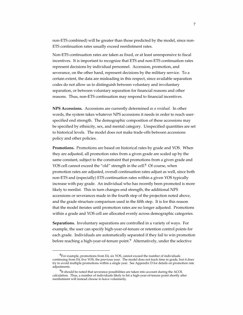
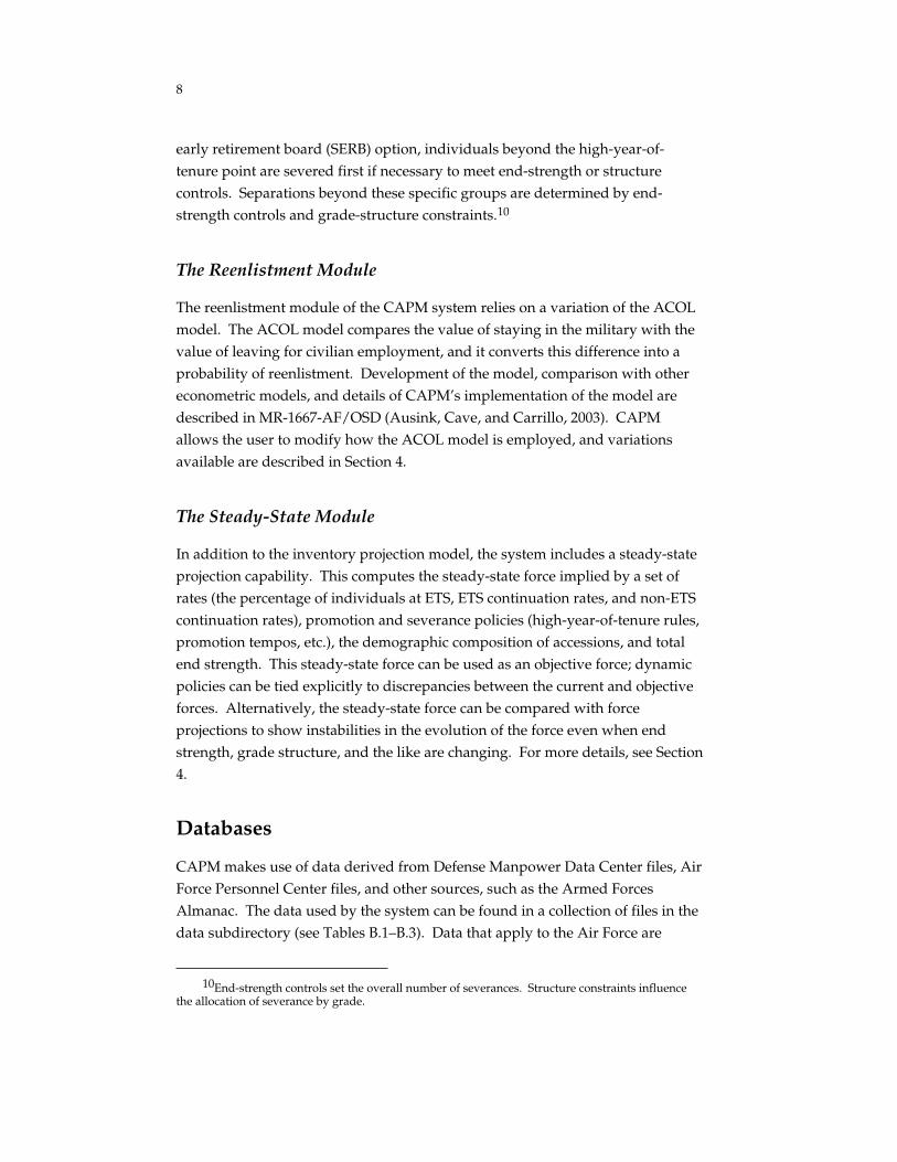
The main CAPM toolbar is displayed horizontally along the bottom of the screen when the program is first opened (see Figure 3.1). Table 3.1 explains the buttons available in this toolbar.

Figure 3.1—CAPM Screen

11

Table 3.1

Main Toolbar

Icon Tip Text Function Help Opens online version of CAPM help

file New Integrated Scenario Opens a new, blank, scenario file Open Existing Input File... Opens an existing input file Open Disaggregated Output File... Opens a disaggregated data output file Open Existing Comparison Sheet... Opens existing “run comparison” file Compare two runs... Shows dialogue for comparison of

output files Context-Sensitive Graphs... Shows context-sensitive graphs of

output data Quit Ends session. Prompts users to save

changes Hide/Unhide all files (toggle) Hides or shows all files Close non-essential files... Closes all files except program files Inject selected data into scenario Records path to selected data in

scenario sheet Steady-state projection Shows context-sensitive steady-state

projections Toggle display of accession Displays (or hides) the toolbar for the toolbar Accessions modulea

Database maintenance/inspection Shows database maintenance dialogue

In

Inject

D ata

Help

New

Out Comp Compare

G raph

Quit

Hide Clean

S teady

S howAcc

aThis module is not currently available.

Dialogue Boxes

During a typical CAPM session, a variety of dialogue boxes assist in setting up options to perform analysis and display results in the way desired by the user. These boxes include the following:

• ACOL Only (used when calculating ACOL values without inventory projections).

• Aggregate Data Graph (used to display aggregate data).

• IPM Only (for inventory projection model runs without ACOL calculations).

• New Pay Element.

• Run Comparison (used for analyzing the effects of policy changes).

• Scenario Initialization (used at the beginning of a session).

• Steady-State Projection (used to determine when, if ever, policies will lead to an inventory that does not change from year to year).

Full descriptions of the functions of these dialogue boxes are found in Section 4.

12

Graphic Controls

In addition to the toolbars and dialogue boxes, several worksheets in the model have other buttons or graphic objects that allow the user to adjust parameters. For example, the worksheet that opens when a user sets up a new scenario includes “command” buttons for initializing, saving, or graphing information related to analysis; “radio” buttons that control the mathematical characteristics of a model used; and other buttons that allow the user to display, change, and hide parameters underlying the analysis.

CAPM Workbooks

Scenarios

The heart of the CAPM system is the scenario sheet. In essence, it is a spreadsheet that contains all data needed to perform a model run.11 When the system is run, the outputs are recorded in the scenario sheet. The sheet also contains controls that allow the user to manipulate files, adjust parameter settings, run some or all models, and inspect outputs. These controls help the user see the effects of a policy change and make related runs to test the robustness of results. The scenario sheet can be thought of as a tool for navigating through “scenario space” or investigating a very complex “response surface.”

Comparison Workbooks

Many policy studies require comparison of a policy case with a base case. To facilitate such comparisons, CAPM offers graphical and numerical comparison workbooks. When a comparison of two cases is done, a worksheet is displayed that allows the user to select comparisons of ACOLs, reenlistment rates, continuation rates, and several other items of interest. These comparisons are initially stored numerically in “pivot” tables, but if the user graphs the data, the graph is stored in an additional worksheet of the workbook.

11For large data blocks (inventories, continuation rates, etc.), the scenario sheet simply records the location of the data in the database or other files. These “pointers” are then passed to the program. This eliminates data duplication and greatly reduces the size and clumsiness of scenario files.

13

Inspecting Results

Tables

The primary method used by CAPM to display results of a model run is the Excel pivot table. An example of CAPM pivot table output is given in Section 4. Data for the pivot table are stored in a hidden worksheet named “Pivot” in the scenario’s *.out file. This worksheet is also discussed in more detail in Section 4.

Graphs

CAPM pivot table outputs automatically include a button to graph selected data. Default settings are generally for bar graphs, but it is easy to use the Excel “Chart” menu to modify graphic outputs as desired.

14

4. CAPM Functions in Detail

This section describes in detail each element of the CAPM interface.

The Main Toolbar

CAPM displays customized toolbars at the bottom of the screen. The functions of the 14 tools and toolbar buttons shown in Table 3.1 are described below.

Help

This button calls up an online help file version of this users’ guide.12

New

This control opens a new scenario file. Selecting this command will cause a scenario worksheet to be displayed. The worksheet will present the file manipulation, parameter setting, model run, and output inspection tools necessary for a model run.

In

This control allows users to open a scenario sheet that has been prepared but not yet used as the basis for a projection. Users can then modify the sheet or run the projection. When this button is selected, users are presented with a “File Open” dialogue box listing the names of all input files in the “User” directory. Users can also choose files from another directory or disk. If a file opened in this way is saved using Save on the scenario sheet, it will be placed in the “User”

directory. All files related to a scenario share a common label. If a scenario is given the label “Test,” for example, the input scenario is named “Test.in.” When the system is run and outputs are added to the file, it is renamed “Test.out.”

Out

This button presents a dialogue box that permits a scenario file containing output data to be opened. When a scenario sheet (say “Test.in”) is run, output data are added, the original input file is deleted (to save disk space), and the results are saved as, e.g., “Test.out.” Generically, we refer to output files as “*.out” files,

12Not functional in the CAPM 2.2 release.

15

since they all have the extension “.out.” Once open, the outputs can be inspected, graphed, exported, etc. In addition to the input data, an output file contains detailed breakdowns of ACOL values, reenlistment rates, inventories, and promotion tempos by grade.

Comp

This button allows the user to open a workbook containing data from a previously run comparison.

Compare

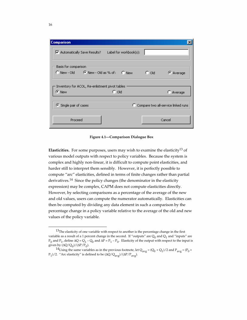
Many policy studies require comparison of a policy case and a base case. To facilitate such comparisons, CAPM offers graphical and numerical comparison workbooks. When this button is selected, the user is presented with the dialogue box (shown in Figure 4.1) that allows comparisons of data located in different *.out files. This dialogue box is used to create a new comparison. In the “Basis for comparison” block, the user can choose to compare the new and old scenarios by calculating the differences in output values (New - Old) or by differences in output values expressed as a percentage of the new or old values (New - Old as % of:). The differences can also be expressed as a percentage of the average of the new and old values. When “Proceed” is pressed, a list of available *.out files is displayed and the user is asked to select a “New” case and an “Old” case for the comparison. The results of the comparison are placed in a workbook. If the Automatically Save Results? box is checked and a label is entered in the text box (e.g., “Test”), the results will be saved as “Test.xlw.”

Inventory for ACOL and Reenlistment Pivot Tables. In examining a pivot table for inventories, users will notice that cell numbers are calculated by adding up across individual tables. That is, the value in the YOS 5 cell for FY00 (fiscal year 2000) would be the sum of the inventories of each grade in YOS 5 in FY00. ACOL values and reenlistment rates cannot be treated so simply. For example, simply adding the reenlistment rates of all grades for YOS 5 in FY00 will not give a meaningful reenlistment rate; instead, the rate must be calculated as a weighted average: Rates are multiplied by populations, the products are added, and the sum is divided by the total population. When comparing two files, the total population in a pivot table cell will likely be different in each file, so when computing the change in reenlistment rate, the user is allowed to select which population to use as the “base value” (denominator) in the calculation. More details on these calculations for the pivot tables in comparison files are provided below.

16

Figure 4.1—Comparison Dialogue Box

Elasticities. For some purposes, users may wish to examine the elasticity13 of various model outputs with respect to policy variables. Because the system is complex and highly non-linear, it is difficult to compute point elasticities, and harder still to interpret them sensibly. However, it is perfectly possible to compute “arc” elasticities, defined in terms of finite changes rather than partial derivatives.14 Since the policy changes (the denominator in the elasticity expression) may be complex, CAPM does not compute elasticities directly. However, by selecting comparisons as a percentage of the average of the new and old values, users can compute the numerator automatically. Elasticities can then be computed by dividing any data element in such a comparison by the percentage change in a policy variable relative to the average of the old and new values of the policy variable.

13The elasticity of one variable with respect to another is the percentage change in the first variable as a result of a 1 percent change in the second. If “outputs” are Q0 and Q1 and “inputs” are P0 and P1, define ∆Q = Q1 – Q0 and ∆P = P1 – P0. Elasticity of the output with respect to the input is given by (∆Q/Q0)/(∆P/P0).

14Using the same variables as in the previous footnote, let Qavg = (Q0 + Q1)/2 and Pavg = (P0 + P1)/2. “Arc elasticity” is defined to be (∆Q/Qavg)/(∆P/Pavg).

17

Graph

This button opens an options box that allows the user to select a variety of data to be graphed. Options include Inventory, Reenlistments, ETS Continuation Rates, ACOLs, Accession Costs, NPS Accessions, and Total Costs.

Quit

This control closes all files and ends the CAPM session. If any files besides database files and the CAPM program files have been modified, users will be asked whether they wish to save the changes.

Hide

This control hides all spreadsheets but leaves the custom toolbar visible.

Clean

This control closes all files except the CAPM.XLS spreadsheet.

Inject

This button is used to modify input data by inserting a pointer to data sources other than default values.

Steady

This control runs the steady-state inventory projection model.

ShowAcc

This control displays (or hides) the toolbar for the Accessions module.15

Data

This control opens a dialogue box that allows the user to select and inspect data files used by CAPM.

Workbook Objects

CAPM uses graphic objects to allow the user to adjust settings, and it organizes many of the detailed setting options in “outlines” that can be expanded by the user.

15This module is not currently available.

18

Graphic Objects

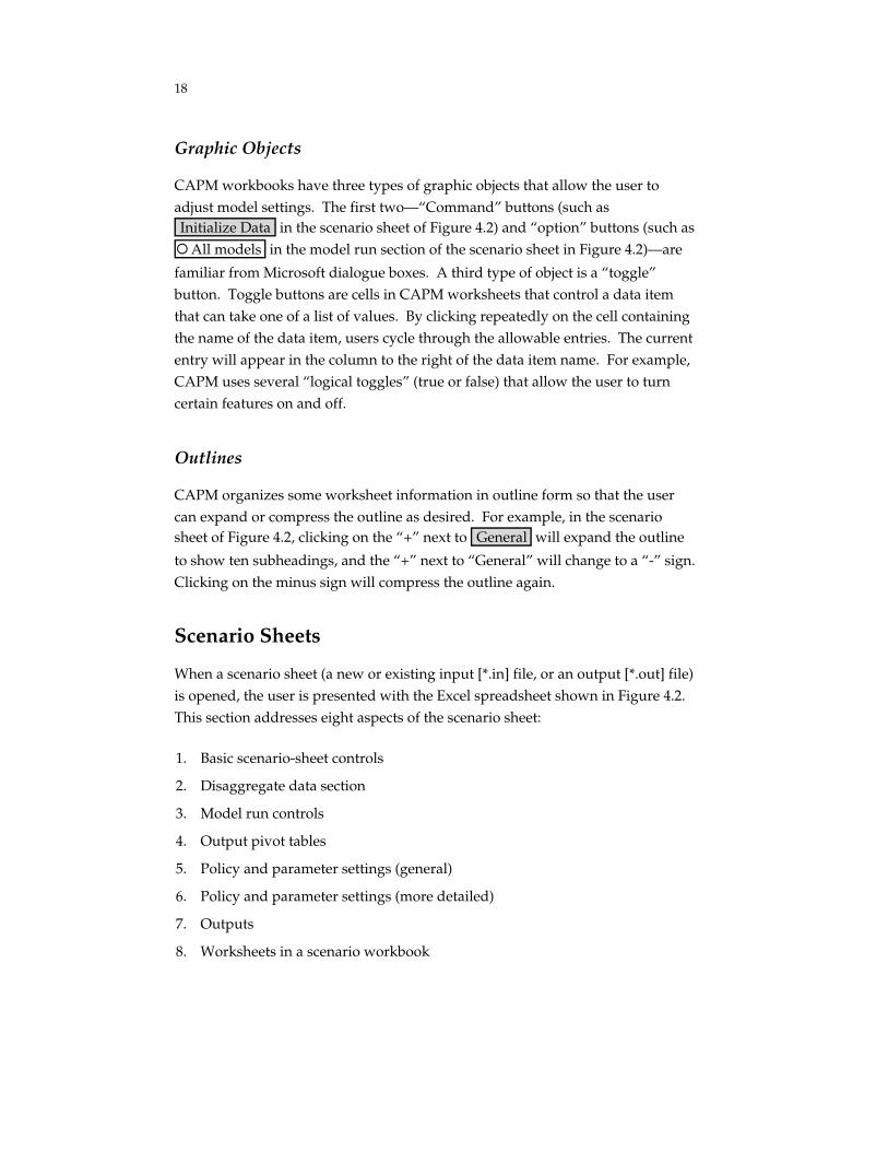
CAPM workbooks have three types of graphic objects that allow the user to adjust model settings. The first two—“Command” buttons (such as Initialize Data in the scenario sheet of Figure 4.2) and “option” buttons (such as � All models in the model run section of the scenario sheet in Figure 4.2)—are

familiar from Microsoft dialogue boxes. A third type of object is a “toggle” button. Toggle buttons are cells in CAPM worksheets that control a data item that can take one of a list of values. By clicking repeatedly on the cell containing the name of the data item, users cycle through the allowable entries. The current entry will appear in the column to the right of the data item name. For example, CAPM uses several “logical toggles” (true or false) that allow the user to turn certain features on and off.

Outlines

CAPM organizes some worksheet information in outline form so that the user can expand or compress the outline as desired. For example, in the scenario sheet of Figure 4.2, clicking on the “+” next to General will expand the outline

to show ten subheadings, and the “+” next to “General” will change to a “-” sign. Clicking on the minus sign will compress the outline again.

Scenario Sheets

When a scenario sheet (a new or existing input [*.in] file, or an output [*.out] file) is opened, the user is presented with the Excel spreadsheet shown in Figure 4.2. This section addresses eight aspects of the scenario sheet:

1. Basic scenario-sheet controls

2. Disaggregate data section

3. Model run controls

4. Output pivot tables

5. Policy and parameter settings (general)

6. Policy and parameter settings (more detailed)

7. Outputs

8. Worksheets in a scenario workbook

19

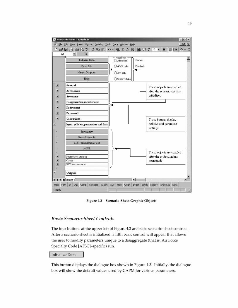
Figure 4.2—Scenario-Sheet Graphic Objects

Basic Scenario-Sheet Controls

The four buttons at the upper left of Figure 4.2 are basic scenario-sheet controls. After a scenario sheet is initialized, a fifth basic control will appear that allows the user to modify parameters unique to a disaggregate (that is, Air Force Specialty Code [AFSC]–specific) run.

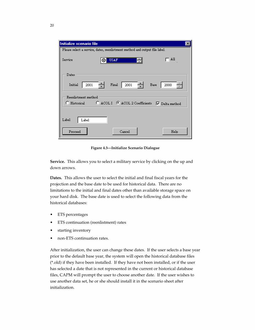
Initialize Data

This button displays the dialogue box shown in Figure 4.3. Initially, the dialogue box will show the default values used by CAPM for various parameters.

20

Figure 4.3—Initialize Scenario Dialogue

Service. This allows you to select a military service by clicking on the up and down arrows.

Dates. This allows the user to select the initial and final fiscal years for the projection and the base date to be used for historical data. There are no limitations to the initial and final dates other than available storage space on your hard disk. The base date is used to select the following data from the historical databases:

• ETS percentages

• ETS continuation (reenlistment) rates

• starting inventory

• non-ETS continuation rates.

After initialization, the user can change these dates. If the user selects a base year prior to the default base year, the system will open the historical database files (*.old) if they have been installed. If they have not been installed, or if the user has selected a date that is not represented in the current or historical database files, CAPM will prompt the user to choose another date. If the user wishes to use another data set, he or she should install it in the scenario sheet after initialization.

21

Reenlistment Method. This section allows users to choose among four methods to determine reenlistment rates. The first uses historical rates without modification. Other options are based on variations of the ACOL model. The main differences are as follows:

• The ACOL I model ignores selection—e.g., it ignores the fact that individuals with a low taste for military service are progressively removed with each reenlistment. The ACOL 2 model adjusts for selection based on an assumption about individual tastes that do not change over time. (See Ausink, Cave, and Carrillo, 2003, or Black, Moffitt, and Warner, 1990a, for details on how estimation of ACOL 2 parameters accounts for selection.)16

• When parameters for the ACOL I model were estimated, civilian income prospects were assumed to depend only on the age at which an individual leaves military service. The ACOL 2 estimates of civilian income take into account both military and civilian experience.

• The ACOL I model includes demographic variables in the regression equation, which converts ACOL values to reenlistment rates, while the ACOL 2 model takes account of demographic variables in the civilian pay stream projection.

• If the Delta method switch is on (checked), the model uses the change in ACOL values induced by a policy change and the ACOL coefficient to calculate the change in reenlistment rate. (See Ausink, Cave, and Carrillo, 2003, for details.) This is the only method available for the ACOL 2 coefficients. If the Delta method switch is off (unchecked), reenlistment rates in the ACOL I model are projected using the original regression equations. That is, if a policy change affects ACOL values, the new values are “plugged into” the regression equation and a reenlistment rate is calculated.

Label. This allows the user to select a text label for the scenario. The label should be 16 characters or fewer in length. Spaces are not allowed in the name, but “underscore” characters are. For example, “Test_Run” would be acceptable, but “Test Run” would not. The program will prompt the user to change the name if the one selected is too long.

When Proceed is pressed, the system will initialize all data and set up the

output ranges corresponding to the run dates the user has chosen. Messages about the progress of initialization will appear at the bottom left of the screen, and the word “Ready” will appear there when the initialization is complete.

16While the ACOL I option is available in CAPM 2.2, the ACOL coefficients are out of date. The ACOL I option has been left in the model in anticipation that the coefficients will be reestimated.

22

If the user initializes an input or output sheet that is already set up, the macro will clear all output ranges and create new ones if necessary. It will also reset all data to default values, keeping only the label, service, and date information.

Save File

This control saves the current file using the label supplied under the General

options setting. That is, if the label is “Test,” the file will be saved as “Test.in.” This will be true even if the open file is an output file; “Test.out” will be saved as “Test.in.” Since *.in files are replaced with *.out files when a projection is made, the process of rerunning a file is simplified and the user is protected against accidental loss of data.

Graph Outputs

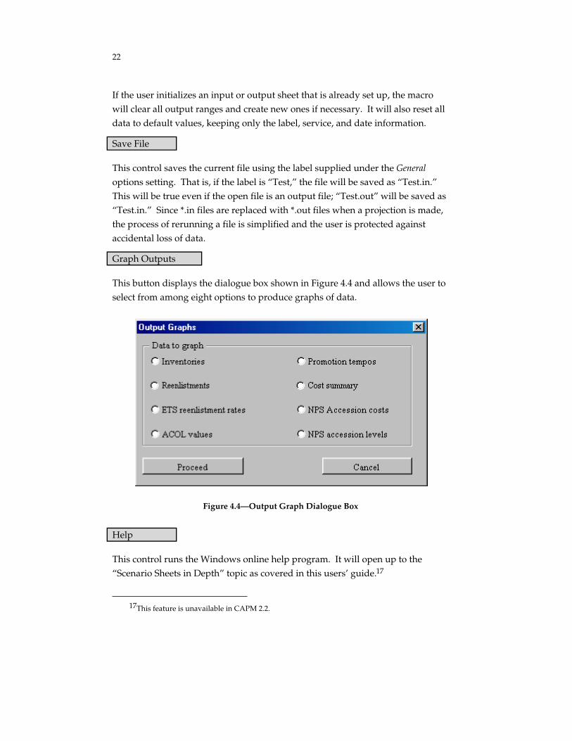
This button displays the dialogue box shown in Figure 4.4 and allows the user to select from among eight options to produce graphs of data.

Figure 4.4—Output Graph Dialogue Box

Help

This control runs the Windows online help program. It will open up to the “Scenario Sheets in Depth” topic as covered in this users’ guide.17

17This feature is unavailable in CAPM 2.2.

23

Disaggregate Data Section

After a scenario sheet is initialized, a new block entitled “Disaggregate Data Section” will appear in the scenario sheet to the right of the model run controls. This block is illustrated in the left half of Figure 4.5.

Disaggregate Data Section

Build New 3-Digit Disaggregate File

Figure 4.5—Disaggregate Data Section

Pressing Build New 3-Digit Disaggregate File will cause the Disaggregate Input

Form to appear (the right half of Figure 4.5). This form allows the user to select a three-digit AFSC for analysis.18 When OK is pressed, CAPM produces a

source file called XXX.dbg (where XXX is the three-digit AFSC) that contains information on the selected AFSC and also sets the scenario sheet so that population data are obtained from XXX.dbg. Because most individual AFSCs have relatively small populations, it is highly likely that some combinations of YOS, grade, and demographic category will contain few, if any, people. Calculating continuation rates and reenlistment rates using these unpopulated cells can lead to questionable results. However, the Disaggregate Input Form allows the user to select the calculated disaggregate values and to set default values if cells have no one in them. If a box is not checked, CAPM will automatically set up the scenario sheet to use the appropriate rate found in the USAF.dbg file for the aggregate population.

18The default file that contains disaggregate information for all AFSCs is rand2000.xls. The user can, if desired, set up an alternate file using the same format.

26

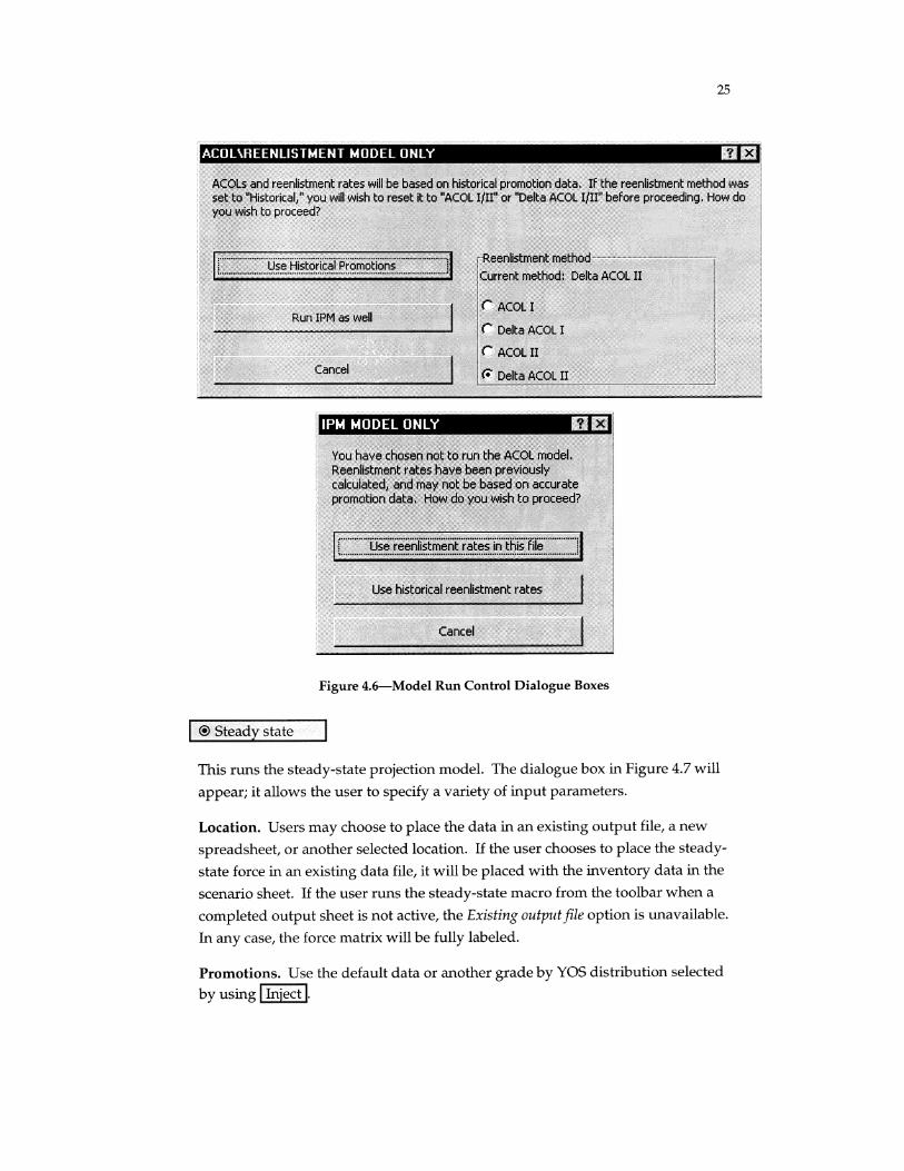
Figure 4.7—Steady-State Dialogue Box

End Strength. Insert a number or, if running the steady-state model from a completed output file, pick one of the projected end strengths.

Reenlistment Rates, ETS Distribution, and Non-ETS Continuation Rates.

Users may choose data (by selecting a fiscal year) from the database. Alternatively, data may be selected by using Inject . If the data lack

demographic data, the YOS 0, and/or YOS 31 fields, the system will supply the data.

NPS Accession Composition. The mix of ethnicity, sex, and mental aptitude is initialized from the projection data or the database file for the service selected by the user. The numbers can be changed using the edit box provided. The numbers must be entered as decimals. In Figure 4.7, the aptitude value of 0.8 means that 80 percent of the accessions must be in the “high” aptitude category.

Grade Controls. These data may be selected from the projected data by year or edited directly. To alter them, select the number to change using the drop-down box in the “Old” row. The number will appear in both the “Old” and “New” boxes. Type a new number in the “New” box and select HYT (for high year of

27

tenure) or Tempo (for promotion tempo) option directly above. The new value

will then appear in the list.

Output Pivot Tables

Excel 97 and later versions offer built-in “pivot table” capabilities. Once the model is run, the buttons labeled Inventory ,

ACOL Reenlistments ,

ETS Continuation Rates , and may be used to create or view pivot

tables of the indicated data. Figure 4.8 shows a sample inventory pivot table.19

Figure 4.8—An Inventory Output Pivot Table

Instructions for working with Excel pivot tables may be obtained by pressing the F1 key to invoke Excel online help and looking under the PivotTable topic. Essentially, each drop-down list controls a field (Demographics, Fiscal Year, YOS, and Grade). The list can be used to toggle display of specific field categories. The two fields listed at the top (described in cells A1 and A2 and

19The data source for the pivot tables is a hidden worksheet named “Pivot,” which can be examined by clicking on “Format” on the Excel toolbar, then “Sheet,” “Unhide,” and then selecting the Pivot worksheet. The columns of this worksheet are ETSCR0 (the end-of-term-of-service continuation rate), Inventory, Reenlistments, ACOL0 (the ACOL value), ETSCR1 (ETSCR0 multiplied by the inventory for a given population), and ACOL1 (ACOL0 multiplied by the inventory for a given population).

28

listed in cells B1 and B2) are called “page fields”; they change the data displayed in the entire pivot table. The fields listed in cells A5 and B4 are the row and column fields, respectively. The field listed in cell A4 is the data field and describes the numbers shown in the body of the table. Users can alter the structure of the table by “dragging” different field names to the page, row or column areas, or into the body of the table.

The ACOL and ETS continuation rate data are presented as population-weighted averages. To see what this means, suppose the pivot table is trying to compute the ACOL value for individuals with grade E5 and YOS 12. For each of the eight demographic categories,20 it multiplies the ACOL value by the corresponding number of individuals. These eight numbers are added, and the sum is divided by the total number of people in grade E5 at YOS 12.21 When the number of people is 0, the pivot table will display the value “#DIV/0!”—this shows up as 0 in the associated graph.22 Before pasting pivot tables into other applications, it may be useful to replace “#DIV/0!” with a blank string or a more intuitive indicator such as “N/A.” This change must be done in the other application, or by copying the values and formats of the pivot table into another location in Excel. To do the latter, follow these instructions:

• Select the pivot table by single clicking the data field cell.

• Copy by using Edit/Copy from the menu, ctrl+C or ctrl+Insert from the keyboard, or the Copy tool from the Excel standard toolbar.

• Select another location and use the menu commands Edit/Paste Special/Values

and Edit/Paste Special/Formats, followed by the Escape key.

• Using the Menu command Edit/Replace, type #DIV/0! in the first text box, leave the second text box blank, and click .Replace All

The YOS field is shown sorted in logical order. Unfortunately, Excel treats field labels as strings of letters rather than numbers and thus orders YOS as YOS 0,

20The categories include all combinations of men and women, white and non-white, and high or low mental category. For example, NFL is non-white, female, low mental category; WMH is white, male, high mental category.

21The product of the ACOL value and the number of individuals is the value ACOL I mentioned in footnote 19. When setting up the pivot table, CAPM also creates the “calculated field” called ACOLs, which is equal to (ACOL1/Inventory). The pivot table is then defined so that the entries are “Sum of ACOLs,” and this value is the weighted average. The ETS Continuation Rate pivot table performs a similar calculation, using the calculated field Reenlistment Rates = (ETSCR1/Inventory).

22Weighted average values of the ACOL numbers are not always appropriate. For example, the analyst may be interested in the average ACOL for a given YOS. To examine this, use the Pivot Table Wizard feature of Excel and replace the “ACOLs” button in the table with the “ACOL0” button. Then use the “field settings” button of the pivot table toolbar to change the calculation of table entries from “sum” to “average.”

29

YOS 1, YOS 10, YOS 11, . . . YOS 2, YOS 20, etc. To correct this, CAPM creates a custom sort order for use with these data. When manipulating a pivot table, users may find that the data revert to the Excel sort order. If this happens, the logical sort order may be restored as follows:

• Select the gray cell containing the text “YOS.”

• Using the Excel menu, select Data/Sort.

• In the resulting dialogue, press Options .

• The logical sort order can be selected from the bottom of the list shown under the heading First key sort order. Select it and press on both

dialogues.

OK

Users may also find it useful to adjust the number formatting and column widths of the pivot table. The data can be graphed by pressing located in cells

D1 through E1. This produces a labeled graph of the data as shown in the pivot table, reflecting any changes made. The label shows the settings of all page fields and the chosen row and column fields.

Graph

With Excel 2000, Graph produces a “pivot graph” that has the same capabilities

as the pivot table, such as drop-down lists for each field and the ability to change fields and chart arrangements by dragging items.

In all Excel versions, the graph includes two additional buttons.

produces a series of graphs corresponding to the various values of a user­selected page field. In the graph corresponding to the data in Figure 4.8, for instance, the user can cycle through the grade-by-YOS inventory profiles for various demographics groups or fiscal years to obtain a clear indication of how

Cycle fields

the force evolves. Delete Graph removes the graph from the scenario sheet.

Policy and Parameter Settings: General Issues

In general, CAPM input data are displayed in an Excel spreadsheet with entries in one column naming the data item and entries in following columns containing information about the data, an address for the data, or a statement about the data. The following are several ways the data elements can be changed.

Numerical Input. These are numerical fields. To alter the data, simply type the new number into the field. To restore the data to its default or database value, clear the data field and click on the cell with the data title.

30

Dialogue Boxes. Clicking on the cell containing the name of some data items will cause a dialogue box to open. Dialogue boxes contain a brief explanation, a text box where users can enter text or numerical data, and buttons that allow users to proceed with or abort the change. Numerical data will be formatted automatically. For example, users can enter a 10 percent interest rate as “10%,” “0.10,” “.1,” etc., without ambiguity.

Toggles. As mentioned above, toggles control a data item that can take one of a list of values. By clicking repeatedly on the cell containing the name of the data item, the user cycles through the allowable entries.

Inject is used to update large data matrices such as continuation rates or

inventories. These data are not copied directly into the scenario sheet. Instead, their location is recorded as a text string to the right of the data item name. At run time, a “soft pointer”—an Excel external reference—is created that points to the actual data. This reference avoids the need for multiple copies of the same data and keeps the size of scenario files down to a reasonable level. Clicking on the data item name causes a dialogue box to appear, indicating that the item has a default setting and allowing the user to retain the default or select a new setting. If a new setting is selected, a message will appear in the bottom left­hand corner of the screen instructing the user to select a data range for the new information. When this message appears, the user can open a spreadsheet containing the desired data,23 select the new data (just the numbers, not the titles or labels), and either

• hold down the control key (Ctrl on most keyboards) while pressing the “s” key or

• click Inject on the CAPM custom toolbar at the bottom of the screen.

To cancel the change, simply ignore the message. It will go away when the user changes to another data item. However, be sure not to hit ctrl+s or Inject at an

inappropriate point. Some safeguards are built in. The macro checks to see whether the user has selected a data range of the right size for the data element being updated.

Users should also be careful about copying scenario sheets to other locations. On a Windows-based computer, the pointers will only update if the copy takes place within a logical partition on the hard drive or if the directory structure pointing

23Make sure that the data are located in the CAPM/Data directory.

31

to the data on the new drive is the same as that on the old drive.24 To illustrate, suppose that the file “D:\Capm\User\Test.in” had a link to the file “D:\Capm\Data\Policy.db.” If you copied “Test.in” to the D:\New directory, the file link would still be “D:\Capm\Data\Policy.db.” However, if you copied “Test.in” to the C:\ drive, as “C:\Test.in,” say, the file link would be “C:\Capm\Data\Policy.db.” If this new file did not exist, the system would produce an error. To be sure that copies to another directory update correctly, the File/Links/Change command from the Excel menu bar should be used. Simply select each inappropriate link in turn, click Change, and use the file box to select the original data file. Then press OK, and resave the scenario file. If you are not sure whether a linked file exists, select the Excel File/Links command, highlight the file in question, and click Update . If Excel cannot find the file, it will

prompt the user to select a new link.

To restore an item to its database default value after using Inject to change it,

clear the item (select the cell where the text address of the item is stored—usually to the right of the item title—and press backspace followed by return). Then click on the cell with the name of the data item.

Note on the Use of Aggregated Data. When Inject is used to change data, the

program keeps track of the necessary number of rows and columns for the data set. If the range selected is not of the correct size, the system will generally remind the user of the appropriate size and provide the opportunity to reselect the data. However, if the user selects a life table that does not make demographic distinctions (see “Life-Table Source” below), the system will automatically copy the life-table data across the demographic categories.

Policy and Parameter Settings: More Details

With the general details of how to change individual data elements out of the way, we can now discuss the specific categories of data elements available in the outline area of a scenario sheet.

General. There are eight functioning data categories under this heading.

Label (dialogue box): the text label of the specific file.

Service (toggle): the service to which this scenario file applies. To change it, click the word “service” in the left-hand column. Clicking this word repeatedly will

24To see whether a copied file will work successfully, select the File/Links command on the Excel menu bar, and see whether the linked files exist.

32

cycle through the four service names; the current name appears to the right of the word “service.”25

Begin Projection (dialogue box): the first year that will be projected. It should normally be the next year after the starting inventory base date. The reason lies in the way the fiscal year enters the projection. In addition to selecting historical data elements, the fiscal year triggers certain policy provisions (notably retirement plans).

End Projection (dialogue box): the last year to be projected. The only limit to run length is storage capacity.

Interest Rate (dialogue box): the interest rate used to calculate the present value of retirement liabilities. Next to the interest rate field is a button labeled

These options control whether the ACOL

computation discounts the future according to the selected financial discount rate or uses a “psychological” discount rate derived from Matthew Black’s 1983 survey report (Black, 1983) on empirical studies of reenlistment behavior.

Use personal discount rates . Selecting this button changes the label to Use Interest rate to discount future .

Database Date (dialogue box): sets a common date for ETS distribution, ETS and non-ETS continuation rates, and starting inventory.

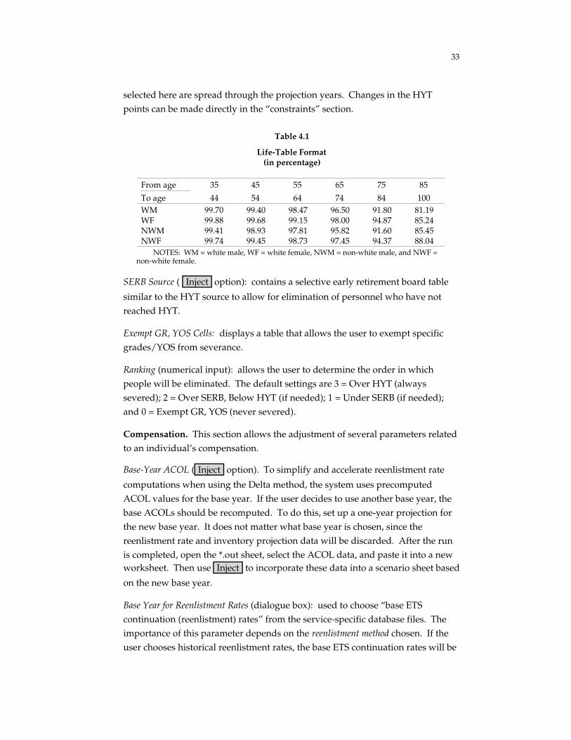
Life-Table Source (“Inject” option): identifies the source of the mortality data used to compute the present value of retirement liabilities for cost calculations. This life table gives conditional survival probabilities by age, sex, and ethnicity. The database table (shown in Table 4.1) is drawn from the U.S. Vital Statistics compendium and gives survival probabilities in ten-year bands. Users may substitute other data as long as the data are similarly configured. To do this, prepare a worksheet containing life-table data as in Table 4.1.

Unemployment Rate (dialogue box): sets the unemployment rate used in the equation that converts ACOL values to reenlistment rates.

Severance. This area allows the adjustment of several parameters related to involuntary separations.

High-Year-of-Tenure Source ( Inject option): sets the high-year-of-tenure or

retention control points used to compute HYT. An HYT table should be a seven-element-column vector of integers, one for each pay grade used. A sample can be found in the “constraints” section of the spreadsheet. The data that are

25With the appropriate data, CAPM can deal with any service, but CAPM 2.2 focuses on the Air Force.

33

selected here are spread through the projection years. Changes in the HYT points can be made directly in the “constraints” section.

Table 4.1

Life-Table Format (in percentage)

From age 35 45 55 65 75 85

To age 44 54 64 74 84 100 WM 99.70 99.40 WF 99.88 99.68 NWM 99.41 98.93 NWF 99.74 99.45

98.47 96.50 91.80 81.19 99.15 98.00 94.87 85.24 97.81 95.82 91.60 85.45 98.73 97.45 94.37 88.04

NOTES: WM = white male, WF = white female, NWM = non-white male, and NWF = non-white female.

SERB Source ( Inject option): contains a selective early retirement board table

similar to the HYT source to allow for elimination of personnel who have not reached HYT.

Exempt GR, YOS Cells: displays a table that allows the user to exempt specific grades/YOS from severance.

Ranking (numerical input): allows the user to determine the order in which people will be eliminated. The default settings are 3 = Over HYT (always severed); 2 = Over SERB, Below HYT (if needed); 1 = Under SERB (if needed); and 0 = Exempt GR, YOS (never severed).

Compensation. This section allows the adjustment of several parameters related to an individual’s compensation.

Base-Year ACOL ( Inject option). To simplify and accelerate reenlistment rate

computations when using the Delta method, the system uses precomputed ACOL values for the base year. If the user decides to use another base year, the base ACOLs should be recomputed. To do this, set up a one-year projection for the new base year. It does not matter what base year is chosen, since the reenlistment rate and inventory projection data will be discarded. After the run is completed, open the *.out sheet, select the ACOL data, and paste it into a new worksheet. Then use Inject to incorporate these data into a scenario sheet based

on the new base year.

Base Year for Reenlistment Rates (dialogue box): used to choose “base ETS continuation (reenlistment) rates” from the service-specific database files. The importance of this parameter depends on the reenlistment method chosen. If the user chooses historical reenlistment rates, the base ETS continuation rates will be

34

used in all projection years. If the user chooses Delta ACOL I or Delta ACOL 2 (the default), historical rates will be adjusted for changes in ACOL. If the user turns off the Delta method option and uses ACOL I, the base ETS reenlistment rates will be ignored.

Base-Year Reenlistment Rates ( Inject option). This parameter allows the user to

specify reenlistment rates outside the database. These reenlistment rates can be used directly (by specifying the “Historical” reenlistment method) or used as the starting point for ACOL adjustment (by specifying the “Delta ACOL 2” reenlistment methods).

Base-Year Unemployment (dialogue box). When the Delta method is selected, CAPM uses ACOL model coefficients to calculate changes in reenlistment rates based on the difference between new ACOL values and stored baseline ACOL values. If the ACOL model being used also has unemployment as a regressor, it is necessary to compare new unemployment rates with baseline unemployment rates as well. This dialogue box lets you insert a baseline unemployment rate for use in this calculation.

Regression Coefficients ( Inject option): a table of service-, demographic-, and

term-specific slope and intercept coefficients used in the ACOL I equation, linking reenlistment rates to ACOL values. The table used reflects the reenlistment method chosen.

Reenlistment Period (numerical input). The ACOL computation offers the individual the choice of leaving the service (thus acquiring any voluntary separation or pension entitlements and joining the civilian pay stream) or reenlisting (and thus collecting any reenlistment bonuses) at periodic intervals. This control sets the number of years for which individuals may reenlist and, thus, the frequency of the ACOL comparison.

Annual Decision After (numerical input): allows the user to specify the year after which the model assumes an individual makes an annual decision to stay or leave. Before this time, an individual makes decisions only if he or she is at the end of a reenlistment period.

Foresight (toggle): determines whether or not individuals anticipate future changes in cost of living adjustment (COLA). Foresight takes the values “perfect,” “constant level” (no COLA), or “constant rate” (continues the current year’s COLA). “Perfect” uses COLAs specified in the Constraints section, continuing the last COLA rate beyond the last projection year. The appropriate COLA assumption is used in the calculation of ACOL values.

35

ACOL (numerical input): the regression coefficient of ACOL used in the ACOL 2 equation, linking reenlistment rates to ACOL values. This input is ignored unless the reenlistment method is Delta ACOL 2.

Constant (numerical input): the regression constant term in the ACOL 2 equation, linking reenlistment rates to ACOL values. This input is ignored with the ACOL 2 Delta method (the default method in CAPM 2.2).

Unemployment Coefficient (numerical input): the regression coefficient on unemployment in the ACOL I or ACOL 2 equation that links reenlistment rates to ACOL values.

Personal Discount Rate ( Inject option). The ACOL model uses personal discount

rates to evaluate pay streams in the future. In the CAPM 2.2 release, these data are drawn from Matthew Black’s survey report (Black, 1983) and are found in the service-specific (*.dbg) database files. An alternative set of discount rates, used in the original OASD/FMP ACOL model, can be found in the Policy.db file.

Selecting this button changes the label to

options control whether the ACOL computations use financial or psychological rates to discount the future.

These rates do not vary by service, and they change much more discontinuously than the survey rates. Other data can also be selected using Inject . Next to the personal discount rate field is a button labeled Use personal discount rates .

Use Interest rate to discount . These

Reenlistment Method (toggle). The CAPM 2.2 release allows four methods to calculate reenlistment rates. The default selection uses the Delta method with ACOL 2 model coefficients estimated by the SAG Corporation (Mackin, 1996) and changes in ACOL values to adjust historical reenlistment rates by grade, demographics, service, and YOS.26 The original OASD/FMP estimation of the ACOL I model is represented by the ACOL I and Delta ACOL I choices. 27

Finally, the user can supply reenlistment rates from historical data or other models for use in the inventory projection model without any further ACOL adjustment. This option is denoted “Historical.” It should be noted that the original ACOL models made no provision for pay grade. CAPM does take account of grade in the ACOL computation; so even the ACOL option will provide reenlistment rates for individuals in a given cohort that increase with pay grade. However, the Delta ACOL 2 and Delta ACOL I options capture

26The Delta method is described by the authors in Ausink, Cave, and Carrillo, 2003. 27The ACOL I coefficients are from a logit estimation done in the early 1990s. The ACOL I

option has been retained in CAPM 2.2 software in anticipation of the availability of updated coefficients.

36

changes in the intercept of the reenlistment rate equation by pay grade as well as by purely financial consequences.

Normal Cost Percentage (numerical input). This is the factor by which basic pay is multiplied to determine the retirement accrual used by the government to take into account future retirement pay obligations.

Compensation Elements. This area under “Compensation” opens up to allow changes to sources for pay and allowances. The user can modify the name of the compensation, the source for information about the compensation, and how the model handles the cost of this compensation.

Name: the text name given to the pay element. Default pay elements are basic pay, regular military compensation (RMC), and civilian pay.

Source: the path describing the location of the data. Associated with this item is an Excel comment field containing seven numerical values. Only the first five are used, and they describe the attributes of the pay data:

• Number of rows the data source has.

• Number of columns the data source has.

• Matrices: Pay elements varying by fiscal year are supplied as a set of separate matrices. To select multiple areas using Inject , hold the Ctrl key

down while selecting each matrix. If the projection length exceeds the number of matrices supplied, the last one is used for all subsequent years.28

• Specificity: whether the item is service specific.

• Type: how the pay element should be handled in ACOL and/or cost computations. The values range from 1 to 10, corresponding to (1) military compensation and cost, (2) military compensation only, (3) military cost only, (4) involuntary severance, (5) reenlistment bonus, (6) civilian pay,(7) voluntary separation, (8) RMC compensation and cost, (9) RMCcompensation only, and (10) RMC cost only.29

28This capability is not available in CAPM 2.2. 29“Military compensation and cost” means that CAPM treats the pay element as basic pay that

an individual receives and that costs the service money. Such pay will affect retirement calculations. “Military compensation only” means that CAPM treats the pay element as basic pay that an individual receives but that does not directly cost the service anything (such as a tax benefit that effectively changes basic pay). CAPM treats “Military cost only” elements as costs to a service that are not received as compensation by individuals (such as per person advertising to increase retention). RMC pay elements will not affect retirement calculations.

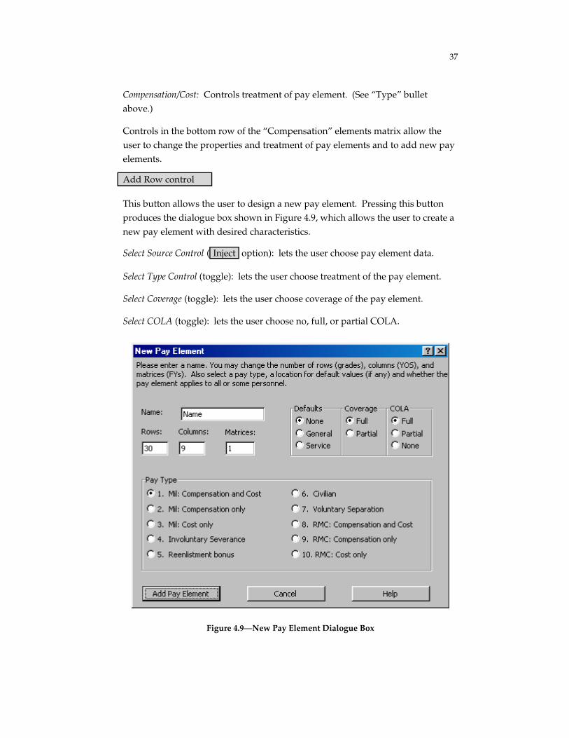
37

Compensation/Cost: Controls treatment of pay element. (See “Type” bullet above.)

Controls in the bottom row of the “Compensation” elements matrix allow the user to change the properties and treatment of pay elements and to add new pay elements.

Add Row control

This button allows the user to design a new pay element. Pressing this button produces the dialogue box shown in Figure 4.9, which allows the user to create a new pay element with desired characteristics.

Select Source Control ( Inject option): lets the user choose pay element data.

Select Type Control (toggle): lets the user choose treatment of the pay element.

Select Coverage (toggle): lets the user choose coverage of the pay element.

Select COLA (toggle): lets the user choose no, full, or partial COLA.

Figure 4.9—New Pay Element Dialogue Box

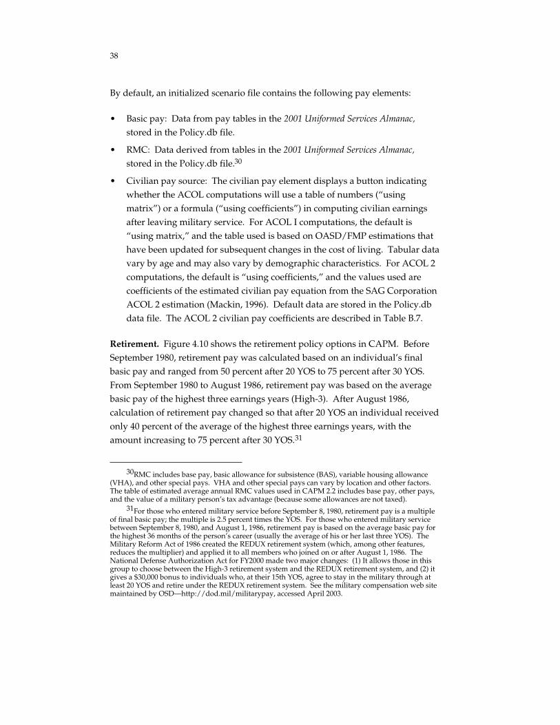
38

By default, an initialized scenario file contains the following pay elements:

• Basic pay: Data from pay tables in the 2001 Uniformed Services Almanac,

stored in the Policy.db file.

• RMC: Data derived from tables in the 2001 Uniformed Services Almanac,

stored in the Policy.db file.30

• Civilian pay source: The civilian pay element displays a button indicating whether the ACOL computations will use a table of numbers (“using matrix”) or a formula (“using coefficients”) in computing civilian earnings after leaving military service. For ACOL I computations, the default is “using matrix,” and the table used is based on OASD/FMP estimations that have been updated for subsequent changes in the cost of living. Tabular data vary by age and may also vary by demographic characteristics. For ACOL 2 computations, the default is “using coefficients,” and the values used are coefficients of the estimated civilian pay equation from the SAG Corporation ACOL 2 estimation (Mackin, 1996). Default data are stored in the Policy.db data file. The ACOL 2 civilian pay coefficients are described in Table B.7.

Retirement. Figure 4.10 shows the retirement policy options in CAPM. Before September 1980, retirement pay was calculated based on an individual’s final basic pay and ranged from 50 percent after 20 YOS to 75 percent after 30 YOS. From September 1980 to August 1986, retirement pay was based on the average basic pay of the highest three earnings years (High-3). After August 1986, calculation of retirement pay changed so that after 20 YOS an individual received only 40 percent of the average of the highest three earnings years, with the amount increasing to 75 percent after 30 YOS.31

30RMC includes base pay, basic allowance for subsistence (BAS), variable housing allowance (VHA), and other special pays. VHA and other special pays can vary by location and other factors. The table of estimated average annual RMC values used in CAPM 2.2 includes base pay, other pays, and the value of a military person’s tax advantage (because some allowances are not taxed).

31For those who entered military service before September 8, 1980, retirement pay is a multiple of final basic pay; the multiple is 2.5 percent times the YOS. For those who entered military service between September 8, 1980, and August 1, 1986, retirement pay is based on the average basic pay for the highest 36 months of the person’s career (usually the average of his or her last three YOS). The Military Reform Act of 1986 created the REDUX retirement system (which, among other features, reduces the multiplier) and applied it to all members who joined on or after August 1, 1986. The National Defense Authorization Act for FY2000 made two major changes: (1) It allows those in this group to choose between the High-3 retirement system and the REDUX retirement system, and (2) it gives a $30,000 bonus to individuals who, at their 15th YOS, agree to stay in the military through at least 20 YOS and retire under the REDUX retirement system. See the military compensation web site maintained by OSD—http://dod.mil/militarypay, accessed April 2003.

39

Add Special Matrices Pre-1981 High3 Redux/High3 First cohort 1900 1981 1987 Last cohort 1980 1986 2500 Vesting YOS 20 20 20 Last YOS 30 30 30 Initial YOS multiplier 50% 50% 40% Max YOS multiplier 75% 75% 75% Vesting grade 1 1 1 Cap grade 1 1 1 Initial grade multiplier 0% 0% 0% Max grade Multiplier 0% 0% 0% Overall max multiplier 75% 75% 75% Initial payment age 0 0 0 Final payment age 100 100 100 Pay basis 0 1 2 Interest/COLA rate 5% 5% 5% Continue after last YOS? 0 0 0 Special Pension Matrix Eligibility matrix

Figure 4.10—Retirement Policy Options

CAPM allows users to design and implement new retirement and voluntary severance formulae. To add a new retirement program, create a new column to the right of the last column of the default retirement matrix, following the instructions given below for the plan’s characteristics. Then click to

ensure that the ACOL and cost models use the new plan. The format given here allows retirement payments to depend on the individual’s final YOS and/or pay grade. Retirement pay is paid in equal amounts over a fixed interval of years. More-complex plans can be modeled by combining many partial plans. For example, a plan that provides a lump-sum payment at retirement and an old-age annuity beginning at age 65 would consist of one plan in which the initial and final payment ages are 0 (representing retirement age), and another plan in which the initial age is 65 and the terminal age is 100.

Reset

The elements of a retirement plan should all be entered manually, and defaults should be used even for options that do not form part of the plan—the retirement matrix should not contain any empty cells.

The actual payment the individual receives for retiring is essentially a sum of a “YOS multiplier” and a “grade multiplier.” To describe the payment calculation in more detail, we will use the shorthand notation shown in Table 4.2.

40

Table 4.2

Retirement Model Notation

Symbol Variable Y0 Vesting YOS G0 Vesting grade N0 Initial grade multiplier Y1 Cap YOS G1 Cap grade N1 Final grade multiplier M0 Initial YOS multiplier M1 Final YOS multiplier

M* Overall max multiplier

An individual who retires at grade G with Y YOS receives a retirement payment that is a multiple of either final basic pay or the High-3 average of basic pay over the last three YOS. The YOS component of this multiplier for a YOS between the vesting and the Cap YOS lies on a straight line between the initial and final YOS multipliers, and similarly for the grade component. The formal expression for this multiplier is

Multiplier = Min{M*, YOS Multiplier + Grade Multiplier}, where (4.1)

0 if

−

and

M Y M Y 00 1 1

<Y Y0 ;min

M1 ,

YOS Multiplier = (4.2)− M0

Y0

+ (M Y1

) * min( Y1, Y) if

− 1 ≥Y Y0

<0 if G G and

0 ;

min

N ,1

Grade Multiplier − −(N ) * min( G , )N G0 1 N G 01 + N G=≥

. G G1 0 1 if

−G1 G0

(4.3)

The rows of the retirement matrix are defined as follows:

First Cohort (numerical input): the entry year for the first-year group covered by the plan. There are no restrictions on the first and last cohorts, provided the last cohort is later than the first. It is possible for more than one plan to apply to a given cohort.

Last Cohort (numerical input): the entry year for the last cohort to be covered by the plan.

0

41

Vesting YOS (numerical input): the minimum number of years of creditable service required to qualify the individual for experience-based retirement payments.

Last YOS (numerical input): the YOS at which the experience multiplier stops increasing.

Initial YOS Multiplier32 (numerical input): the proportion of the payment basis (see below) that the individual receives by retiring at the vesting YOS.

Max YOS Multiplier (numerical input): the maximum YOS multiplier, attained at the “Last YOS.”

Vesting Grade (numerical input): the minimum pay grade at which the individual becomes eligible for responsibility-based retirement payments.

Cap Grade (numerical input): the grade at which the grade multiplier stops increasing.

Initial Grade Multiplier33 (numerical input): the proportion of the payment basis (see below) that the individual gets by retiring at the vesting grade.

Max Grade Multiplier (numerical input): the maximum grade multiplier, attained at the “Cap grade.”

Overall Max Multiplier (numerical input): the maximum sum of the YOS and grade multipliers.

Initial Payment Age (numerical input): the chronological age at which payment of the pension annuity starts. To start payment immediately upon retirement, set this value to 0.

Final Payment Age (numerical input): the chronological age at which payment of the pension annuity ceases. To provide a single lump-sum cash payment, set this value equal to the “initial payment age.”

Pay Basis (numerical input): Enter 0 to pay the individual a multiple of his final basic pay, and enter 1 to pay the individual a multiple of the average of his last three basic pay levels. CAPM 2.2 does not track time in grade, so the basic pay

32To turn off the YOS multiplier, be sure that the initial and final multipliers are set to 0. To create a pension that is a constant multiple of the payment basis in all YOS after the vesting YOS, set the initial and final YOS multipliers equal to each other.

33To turn off the grade multiplier, be sure that the initial and final multipliers are set to 0. To create a pension that is a constant multiple of the payment basis at all grades at or above the vesting grade, set the initial and final grade multipliers equal to each other.

42

levels used under this option assume the individual has held his retirement grade for the previous three years. If the value 2 is entered, the program will use a customized retirement pay matrix as the basis for retirement pay. To introduce such a special matrix, select the cell of the retirement program for which the special matrix will be used. For example, select the cell “Pre-1981.” Next, click on Add Special Matrices . A dialogue box will appear reminding the user to

select a matrix with seven columns corresponding to the seven pay grade levels (E1–E3 counts as a single grade) and 30 rows for YOS 1 to YOS 30. When the matrix is selected, press Inject on the CAPM toolbar to set up the “soft” pointer

to the matrix. The path name to the matrix is recorded in the “Special Matrix” row of the retirement plan specification.

Interest/COLA Rate (numerical input): the COLA rate to be used for individual retirement plans. It should be measured relative to full cost of living adjustment. For example, a COLA plan that adjusts retirement pay by 1/2 the COLA rate would be 1.5 percent if the anticipated COLA rate were 3 percent. By default, this is set equal to 0 (full COLA).

Special Pension Matrix (numerical input): the path name of a special matrix used to define a basis for retirement pay other than final basic pay or High-3. For example, this matrix can be used to represent COLA “catch-up” pay that could not be represented using the standard representation.34

Personnel

Inventory and Rate Data Formats. Inventories, ETS rates, and continuation rates are contained in matrices with 56 rows and 32 columns located in the Policy.db data file. The columns are YOS, numbered from 0 to 31. “0” represents unknown YOS, and 31 represents individuals with 31 or more YOS. The rows combine grade and demographic information as follows. The first eight rows are individuals in pay grades E1–E3, the next eight rows are pay grade E4, etc. Within each grade, the demographics are arranged as shown in Table 4.3. The Policy.db file also contains the information from these matrices in vector form (one column with 1,792 rows).

The expanded “Personnel” section of the outline in the scenario sheet contains the following eight subcategories of data.

34Neither the “Continue after last YOS” row nor the “Eligibility matrix” row functions in CAPM 2.2.

43

Table 4.3

Demographic Coding

Theta (row) Ethnicity Sex Aptitude 1 W M H 2 W M L 3 W F H 4 W F L 5 N M H 6 N M L 7 N F H 8 N F L

NOTES: W = white, N = non-white, M = male, F = female, L = low (aptitude), and H = high (aptitude).

ETS Percentages Source ( Inject option): 56 × 32 matrix showing the proportion

of individuals within 13 months of the end of a term of obligated service. This is used to separate individuals to whom the ETS (reenlistment) and non-ETS continuation rates should be applied. The CAPM 2.2 release does not adjust ETS percentages to reflect changes in reenlistment rates. The data form a matrix whose format is identical to the format of the reenlistment rate and inventory matrices contained in a *.out sheet. The cell to the right of this data name shows the path to the vector form of the data.

Non-ETS Continuation Source ( Inject option): 56 × 32 matrix of continuation

rates to be applied to individuals not facing a reenlistment decision. The cell to the right of this data name shows the path to the vector form of the data.

Starting Inventory Source ( Inject option): 56 × 32 force matrix used to start the

inventory projection. The cell to the right of this data name shows the path to the vector form of the data.

Promotion Rates Source ( Inject option): matrix of promotion rates used by the

model. The cell to the right of this data name shows the path to the matrix of promotion rates.

Fixed Promotion Expectations (toggle): In CAPM’s inventory projection model, promotion rates are adjusted as needed in order to meet user-specified grade­structure constraints or targets. If this toggle is on, individuals are assumed to compute their ACOLs using current promotion rates. If this toggle is off, individuals are assumed to calculate ACOLs using promotion rates that are adjusted by CAPM.

End Strength Control Type (toggle): The default setting for this parameter is “number.” With this setting, CAPM maintains the inventory set in the

44

“Endstrength” parameter of the Constraints section. If the setting is toggled to “percentage,” the projected end strength will be the specified proportion of the previous year’s end strength.

Speed Up Promotions? (toggle): allows the user to specify whether the TOP 4 constraint value (which limits the proportion of the force allowed in grade E4 or above) or the TOP 5 constraint value (which limits the proportion of the force allowed in grade E5 or above) should be treated as a constraint (“False”) or as a target (“True”). In the former case, promotions from E4 and E5 will be slowed down if necessary to meet TOP 4/5 constraints, but they will not be increased beyond their historical levels. In the latter case, promotions will be scaled up or down as necessary to come as close to the TOP 4/5 targets as feasibility allows.35

Grade Structure Control Table: a table showing the type of structure control applied for each grade. Numerical values associated with structure controls are displayed by fiscal year in the Constraints section. The indicator variables here take the values 0 (no structure control), 1 (“TOP X” control limiting the proportion of the force in the current grade or above) and 2 (limits on the proportion of the force in the indicated grade). With the value “1” or “2,” the proportion of the force allowed in a given grade or set of grades will be limited to the value given in the “structure constraints” rows of the Constraints section.

Constraints

This section contains all settings that vary by fiscal year. These include the following:

• fiscal year

• end strength

• minimum NPS accessions (for various demographic categories)

• high year of tenure (by grade)

• SERB (by grade)

• structure constraints for grades E4, E5, E6, E7, E8, E9

• maximum promotion tempo (by grade for E3 to E8)

• minimum promotion tempo (by grade for E3 to E8)

35A promotion pattern is feasible if it does not promote any individual more than one pay grade per year and if it does not promote more individuals than are eligible for promotion.

45

• inflation36

• COLA rates for basic pay, RMC, civilian pay, and retirement

• unemployment.

All data can be modified directly by typing in new values. Most items have been defined earlier or are self-explanatory. A few specific items are described below.

Unemployment (numerical input): used as a separate regressor in the ACOL I model. Given the choice and the data, a rate that matches the unemployment rate for individuals recently leaving military service should be used. However, since the ACOL model does not take explicit account of the likely duration of unemployment for individuals choosing to leave the service, job search costs or the likely impact on civilian wages, precise matching of the unemployment rate within labor market subgroups is probably unnecessary and not helpful.

Maximum and Minimum E4/5 Promotion Tempos (numerical input): The inventory projection model scales promotions from E4 and E5 up or down as required by the TOP 4/5 constraints or goals. These parameters set the overall maximum and minimum amount by which promotion rates can be rescaled. The default maximum is defined by the condition that everyone would be promoted. To avoid speeding up promotions, the maximum promotion scaling factor should be set to 1, in which case historical promotion rates will not be increased. The default minimum is 0.

Outputs

Opening the “Outputs” section of a scenario sheet displays four buttons ( Inventory , , ETS Continuation Rates , and ACOLs ) and threeR eenlistments

subsections of the outline (promotion tempos, costs, and NPS accessions).

Pressing any of the four buttons opens a pivot table containing the corresponding data. The table can be manipulated as desired. The pivot table includes a button labeled Graph that will automatically produce a graph of the

data in the table.

Promotion Tempos. Opening this subsection displays the promotion tempo values stored in the scenario sheet for promotions from E4 and E5. These are the

36In the CAPM 2.2 release, this inflation rate is used in retirement and military pay calculations. A separate inflation rate for civilian pay can be set, but this must be done in the VBA code by adjusting the variable cpinfl in line 224 of the VB_ACOLV2 subroutine, located in Module 4 of the CAPM project. The default civilian inflation value in CAPM 2.2 is 0.053.

46

maximum values by which promotion rates can be multiplied if promotion rates are adjusted during inventory calculations. Appendix D describes these values in more detail.

Costs. Opening this subsection displays values of several summary cost measures for each fiscal year: RMC, retirement liability, non-compensation costs, retirement accrual (the amount the government must show “on the books” to account for potential future retirement obligations), involuntary severance, and reenlistment bonus. If no values are stored, a dialogue box will be shown. Regular military compensation includes basic pay, allowances, special pay, and VHA. Retirement liability is the present value (adjusted for discounting, inflation, and mortality) of the retirement/voluntary severance payments due to individuals retiring in the current year. Dividing retirement liability by basic pay gives a crude measure of the “normal cost percentage” that would prevail if that year’s force were to continue in steady state. Increases or decreases in this percentage over time can signal impending deficits or surpluses in the actual accrual account, and cross-service comparisons can expose implicit subsidies among services.

NPS Accessions. Opening this subsection displays numbers of high-quality and low-quality non-prior-service accessions as determined by the model. NPS accessions are determined as a residual; that is, the model adds as many accessions as necessary to achieve the desired end strength.37

Worksheets in a Scenario Workbook

After a scenario is run, the workbook displayed will be an Excel workbook with the name of the scenario selected by the user and a “.out” extension. Initially, this workbook will have only one worksheet in it, named “Data.” If the user selects the Inventory , Reenlistments , ETS Continuation Rates , or ACOLs

output button, the pivot table created will be placed in a new sheet of the workbook with the corresponding name. If a graph is created from the pivot table, the chart will be placed in another sheet of the workbook with the name “Chart X,” where X is the number of the chart created. The workbook will therefore collect sheets of data and charts that record as much information related to the user’s analysis as desired.

37Individuals in AFQT mental categories IIIA and above are labeled “high quality” in CAPM; individuals in mental categories IIIB and below are labeled “low quality.”

47

Comparison Workbooks

The workbook created when the user conducts a comparison of two scenarios is structured just like a scenario worksheet. Initially, the workbook will contain only one sheet, titled “Data.” The first few rows of the sheet contain information about the “old” file, the “new” file, the first and last fiscal years of the comparison, how the comparison values are calculated, and whether the base inventory used is from the new file or from the old file. Next, there is a “Comparison” outline section that contains the same four buttons and subsections as the “Out” section of the scenario sheet outline. If the user selects the Inventory , Reenlistments , ETS Continuation Rates , or ACOLs output

button, the pivot table created will be placed in a new sheet of the workbook with the corresponding name. If a graph is created from the pivot table, the chart will be placed in another sheet of the workbook with the name “Chart X,” where X is the number of the chart created. As with the scenario workbook, then, the comparison workbook will collect sheets of data and charts that record as much information related to the user’s analysis as desired.

As noted earlier, output information from which the pivot tables are constructed is stored in a hidden sheet called Pivot. In addition to the columns used in a regular output file, the hidden comparison pivot worksheet contains columns of changes in values and columns of weighted values:

• ETSCR0 (the change in ETS continuation rate from the old scenario to the new)

• ETSCR1 (ETSCR0 multiplied by the base inventory selected by the user)

• Inventory0 (the change in inventory from the old scenario to the new)

• Inventory1 (Inventory0 multiplied by the base inventory selected by the user)

• Reenlistments0 (the change in reenlistments from the old scenario to the new)

• Reenlistments1 (Reenlistments0 multiplied by the base inventory selected by the user)

• ACOL0 (the change in ACOL from the old scenario to the new)

• ACOL1 (ACOL0 multiplied by the base inventory selected by the user).

The default setting for a comparison uses “weighted” inventories (the value Inventory1) to compare inventory values with weighted reenlistment values (Reenlistments1) to calculate changes. The pivot table then uses the calculated field “Inventories = Inventory1/Base” for inventory changes and the calculated

48

field “Reenlistments = Reenlistments1/Base” for reenlistment changes. If inventory or reenlistment changes are of special interest, the user should adjust the pivot table by using the Pivot Table Wizard layout feature to change entries from Inventories (or Reenlistments) to Inventory0 (or Reenlistments0).

49

Appendix

A. Installation

Hardware and Software

CAPM 2.2 is designed to run on a Microsoft Windows 98, Windows 2000, or Windows NT4-based personal computer. A minimum of 16 MB of RAM is required; at least 64 MB is recommended. The CAPM 2.2 programs require approximately 3.5 MB of disk space, but 5 MB of free disk space is recommended because of the size of output files (which are typically larger than 1 MB).

The system uses off-the-shelf software to a large extent. The “front end” of the system runs as an Excel 97 or above application with Windows 98 or higher. Numerical computations are carried out by various subroutines written in Visual Basic for Applications. Past experience has shown that care must be taken when upgrading to new versions of Windows or Excel. Users should compare test runs on the new software with older runs to confirm that outputs are being produced properly.

Specific platforms on which CAPM has been tested include the following:

• Dell Precision 420, 933 MHz, 256 MB RAM, 9 GB hard drive, using the Microsoft NT operating system and both Excel 97 and Excel 2000.

• Dell GX-260, 2 GHz, 256 MB RAM, 40 GB hard drive, using the Windows 2000 operating system and Excel 2000. This system was on a network with “user only” access.

• Sony VAIO laptop, 700 MHz, 200 MB hard drive, using the Windows 98 operating system and Excel 97.

Installation

CAPM can be downloaded from RAND’s web site at www.rand.org/ publications/MR/MR1668/. The CAPM folder structure should be downloaded automatically, but the user should check for the following folders and contents:

1. A main folder called “CAPM.”

50

2. Two subfolders within the CAPM folder, one named “USER” and the other “DATA.”

3. The following files should be in the CAPM folder: a. Accessions.xlt b. Capm.xls c. Comp.xlt d. firsttime.xls e. Rand2000.xls f. Scenario.xlt

4. The following files should be in the “DATA” subfolder: a. Payalt.db b. Policy.db c. USAF.dbg

5. The “USER” folder is used for CAPM output and does not initially contain any files.

Before running CAPM, ensure that Excel has the “Solver Add-in” installed. To check this, click on “Tools” on the main Excel toolbar, and then click on “Add­ins.” Scroll down the resulting list to see if the “Solver Add-in” box is checked. If it is not checked, check it and click “OK.” If Solver is not listed in the Add-Ins dialog box, you may have to re-install Excel and select the option to install Solver. After installation, CAPM 2.2 should be started by double clicking on the “firsttime.xls” file in the CAPM folder. This program sets up certain paths for the program. Before quitting CAPM after using it for the first time, save it using File—Save. Subsequently, the user should start CAPM by double clicking on the “Capm.xls” file in the CAPM folder.

Path Names and File Locations

The CAPM root directory contains several files plus the subdirectories CAPM/DATA and CAPM/USER. Table A.1 shows the contents of each directory and subdirectory.38

38Appendix B contains a description of the purpose or contents of each file.

51

Table A.1

CAPM Directory Structure and Contents

CAPM

Program Files Templates Other Files Capm.xls Scenario.xlt Rand2000.xls

Firsttime.xls Accessions.xlt Comp.xlt

CAPM/DATA

Payalt.db USAF.dbg Policy.db

CAPM/USER

*.in *.out

52

B. Inspection, Management, and Structure of Database Files

Inspection of Data Using the Data Button

When Data on the CAPM toolbar is pressed, the dialogue box in Figure B.1 is

displayed.

Figure B.1—Data Inspection and Maintenance Dialogue Box

With this dialogue box, current values of all data can easily be inspected. For example, if “USAF” is the selected service and “ACOL I regression coefficients” is highlighted, the “Dimensions” section of the dialogue box will display the dimensions of the parameter, the “Status” section will note whether or not the CAPM default values for the data item are being used or if they have been changed, and the “Contents” section will provide a brief description of the data.

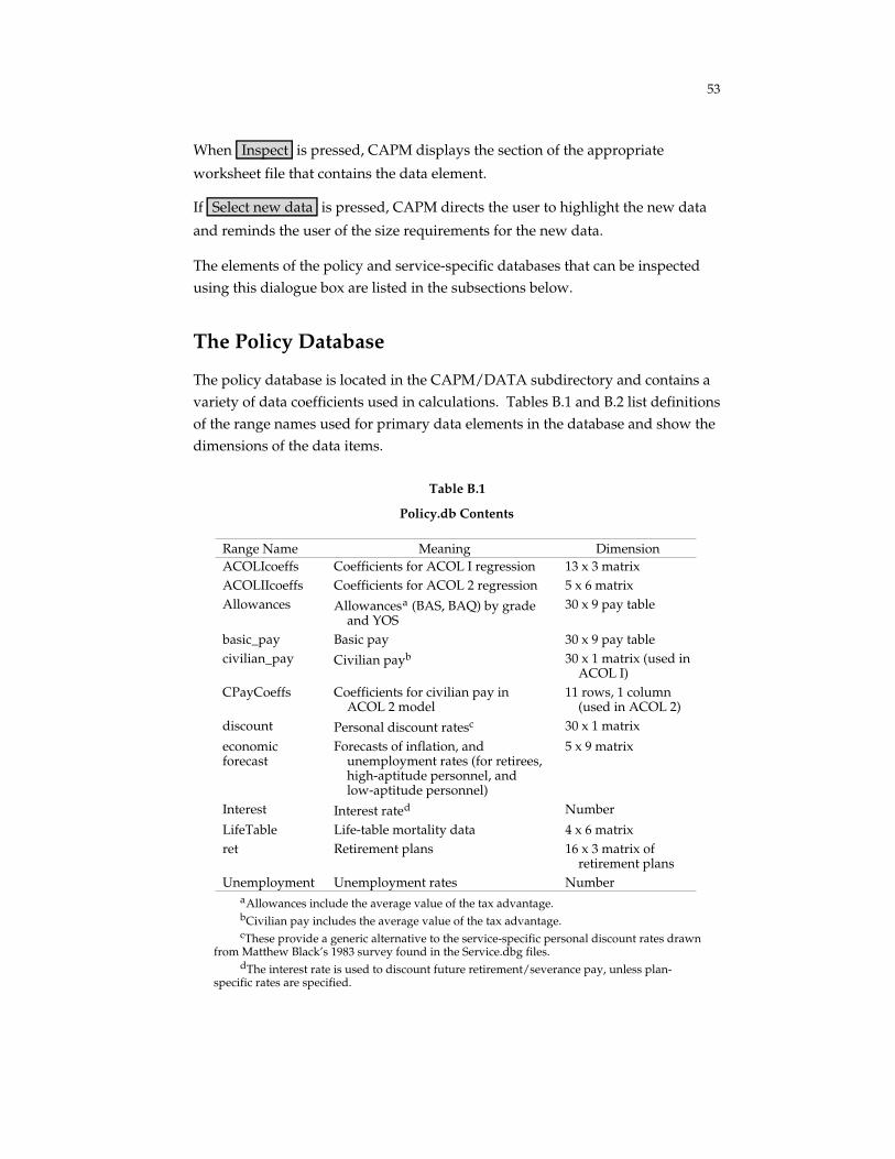
53

When Inspect is pressed, CAPM displays the section of the appropriate

worksheet file that contains the data element.

If Select new data is pressed, CAPM directs the user to highlight the new data

and reminds the user of the size requirements for the new data.

The elements of the policy and service-specific databases that can be inspected using this dialogue box are listed in the subsections below.

The Policy Database

The policy database is located in the CAPM/DATA subdirectory and contains a variety of data coefficients used in calculations. Tables B.1 and B.2 list definitions of the range names used for primary data elements in the database and show the dimensions of the data items.

Table B.1

Policy.db Contents

Range Name Meaning Dimension ACOLIcoeffs Coefficients for ACOL I regression 13 x 3 matrix ACOLIIcoeffs Coefficients for ACOL 2 regression 5 x 6 matrix Allowances Allowancesa (BAS, BAQ) by grade

and YOS 30 x 9 pay table

basic_pay Basic pay 30 x 9 pay table civilian_pay Civilian payb 30 x 1 matrix (used in

ACOL I) CPayCoeffs Coefficients for civilian pay in

ACOL 2 model 11 rows, 1 column

(used in ACOL 2) discount Personal discount ratesc 30 x 1 matrix

economic Forecasts of inflation, and 5 x 9 matrix forecast unemployment rates (for retirees,

high-aptitude personnel, and low-aptitude personnel)

Interest Interest rated Number

LifeTable Life-table mortality data 4 x 6 matrix ret Retirement plans 16 x 3 matrix of

retirement plans Unemployment Unemployment rates Number

aAllowances include the average value of the tax advantage.bCivilian pay includes the average value of the tax advantage.cThese provide a generic alternative to the service-specific personal discount rates drawn

from Matthew Black’s 1983 survey found in the Service.dbg files. dThe interest rate is used to discount future retirement/severance pay, unless plan­

specific rates are specified.

54

P

Table B.2

olicy.db Contents—ACOL Coefficients

Range Name Meaning Dimension AI USAF regression coefficients 25 intercepts AR Army regression coefficients 25 intercepts Base Constant term Number High-Apt. High-aptitude intercept dummy Number MA USMC regression coefficients 25 intercepts NA Navy regression coefficients 25 intercepts NWF Non-white female intercept dummy Number NWM Non-white male intercept dummy Number post80acol Slope dummy Number PostFY80 Intercept dummy Number Term_2 Second-term intercept dummy Number Term_3 Third-term intercept dummy Number UNEMPL Intercept dummy Number USA Army intercept dummy Number USMC USMC intercept dummy Number USN Navy intercept dummy Number WF White female intercept dummy Number

NOTES: Range names in this table refer to coefficients for the ACOL I equation relating ACOL values to retention rates. The “intercept” values are adjustments made to the equation intercept for different populations. The ACOL I equation allows for variation in the intercept by race, sex, mental category (high or low), and term (first, second, or third). Thus there are 24 possible adjustments to the original intercept, for a total of 25.

Service-Specific Databases

Each service has a database called Service.dbg (where “service” can be Army [USA], Navy [USN], Air Force [USAF], or the Marine Corps [USMC]) located in the CAPM/DATA subdirectory. The contents of each service database are listed in Table B.3. Only the Air Force file (USAF.dbg) was updated for CAPM 2.2.

The data in Table B.3 are available for the base fiscal year (2000 in the CAPM 2.2 release).

55

Table B.3

Service.dbg Contents

Range Name Meaning Dimension aprom Promotion rates 31 YOS by 7 grades BASE_ACOL Base-year ACOL values 30 YOS by 7 grades DISCOUNT Personal discount rates YOS 30 Endstrength_targets Planned strength levels Arbitrarya

ES_TYPE “Number” or “percent” Single cell ETS End-of-term-of-service distribution Forceb

ETSCR End-of-term-of-service continuation rates Force Fixed_Cost Fixed accession cost Number High Desired high-aptitude accessions Number

proportion HYT High-year-of-tenure table Grade 7 Male Desired accessions proportion Number MAX_SCALE4 Maximum E4 promotion tempo Number MAX_SCALE5 Maximum E5 promotion tempo Number Min_NPS_targets Minimum NPS accession level Arbitrarya

Min_Sev_targets Minimum severance level Arbitrary NETSCR Non-ETS continuation rates Force NPS Non-prior-service accessions Demographic PS Prior-service accessions Force SINV Starting inventory Force SPAY Special pay Pay table SRB Selective reenlistment bonus (average) Pay table TOP4_targets Percentage in E6–E9 Arbitrary TOP5_targets Percentage in E5–E9 Arbitrary VHA Variable housing allowance (average) Pay table White Desired accessions proportion Number

aThere is one entry for each out-year you wish to specify.bDimensions in this column described by words such as “force” are defined in Table B.4.

Data Formats and File Information

This subsection contains descriptions of the formats used for data elements in the system (Table B.4) and an element-by-element listing in Table B.5 of the names and formats of data items that can be changed using Inject or by changing path

names. These format descriptions can help you set up your own data for incorporation in the model by using Inject . For example, in Table B.5 the

format of allowances.ptr is listed as “pay table.” According to Table B.4, “pay table” means that the data in allowances.ptr are arranged by YOS in rows and by grades in columns.

This subsection also contains values for the ACOL regression coefficients in Table B.6 and coefficients for the civilian pay equation in Table B.7.

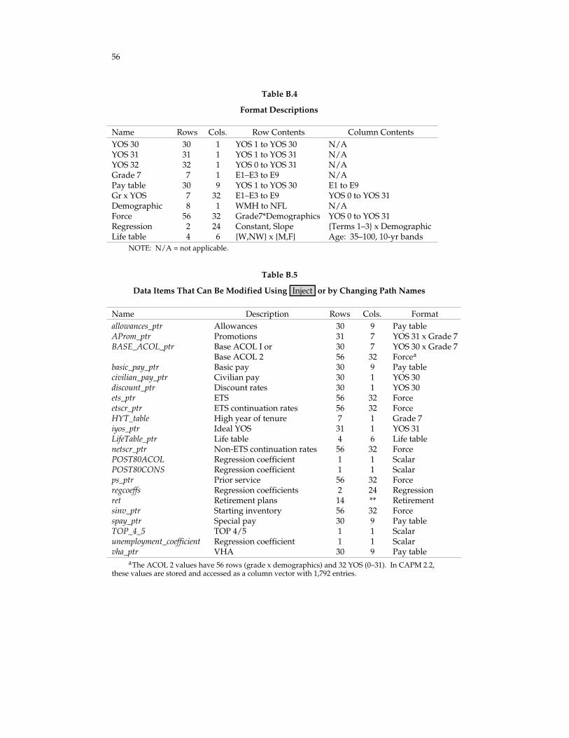
56

Table B.4

Format Descriptions

Name Rows Cols. Row Contents Column Contents YOS 30 30 1 YOS 1 to YOS 30 N/A YOS 31 31 1 YOS 1 to YOS 31 N/A YOS 32 32 1 YOS 0 to YOS 31 N/A Grade 7 7 1 E1–E3 to E9 N/A Pay table 30 9 YOS 1 to YOS 30 E1 to E9 Gr x YOS 7 32 E1–E3 to E9 YOS 0 to YOS 31 Demographic 8 1 WMH to NFL N/A Force 56 32 Grade7*Demographics YOS 0 to YOS 31 Regression 2 24 Constant, Slope {Terms 1–3} x Demographic Life table 4 6 {W,NW} x {M,F} Age: 35–100, 10-yr bands

NOTE: N/A = not applicable.

Table B.5

Data Items That Can Be Modified Using Inject or by Changing Path Names

Name Description Rows Cols. Format allowances_ptr Allowances 30 9 Pay table AProm_ptr Promotions 31 7 YOS 31 x Grade 7 BASE_ACOL_ptr Base ACOL I or 30 7 YOS 30 x Grade 7

Base ACOL 2 56 32 Forcea

basic_pay_ptr Basic pay 30 9 Pay table civilian_pay_ptr Civilian pay 30 1 YOS 30 discount_ptr Discount rates 30 1 YOS 30 ets_ptr ETS 56 32 Force etscr_ptr ETS continuation rates 56 32 Force HYT_table High year of tenure 7 1 Grade 7 iyos_ptr Ideal YOS 31 1 YOS 31 LifeTable_ptr Life table 4 6 Life table netscr_ptr Non-ETS continuation rates 56 32 Force POST80ACOL Regression coefficient 1 1 Scalar POST80CONS Regression coefficient 1 1 Scalar ps_ptr Prior service 56 32 Force regcoeffs Regression coefficients 2 24 Regression ret Retirement plans 14 ** Retirement sinv_ptr Starting inventory 56 32 Force spay_ptr Special pay 30 9 Pay table TOP_4_5 TOP 4/5 1 1 Scalar unemployment_coefficient Regression coefficient 1 1 Scalar vha_ptr VHA 30 9 Pay table

aThe ACOL 2 values have 56 rows (grade x demographics) and 32 YOS (0–31). In CAPM 2.2, these values are stored and accessed as a column vector with 1,792 entries.

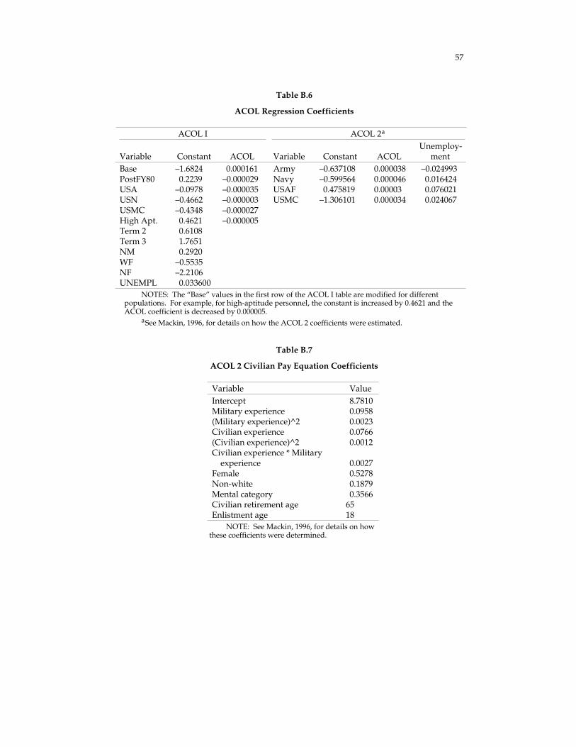
57

Table B.6

ACOL Regression Coefficients

ACOL I ACOL 2a

Unemploy-Variable Constant ACOL Variable Constant ACOL ment Base –1.6824 0.000161 Army –0.637108 0.000038 –0.024993 PostFY80 0.2239 –0.000029 Navy –0.599564 0.000046 0.016424 USA –0.0978 –0.000035 USAF 0.475819 0.00003 0.076021 USN –0.4662 –0.000003 USMC –1.306101 0.000034 0.024067 USMC –0.4348 –0.000027 High Apt. 0.4621 –0.000005 Term 2 0.6108 Term 3 1.7651 NM 0.2920 WF –0.5535 NF –2.2106 UNEMPL 0.033600

NOTES: The “Base” values in the first row of the ACOL I table are modified for different populations. For example, for high-aptitude personnel, the constant is increased by 0.4621 and the ACOL coefficient is decreased by 0.000005.

aSee Mackin, 1996, for details on how the ACOL 2 coefficients were estimated.

Table B.7

ACOL 2 Civilian Pay Equation Coefficients

Variable Value Intercept 8.7810 Military experience 0.0958 (Military experience)^2 0.0023 Civilian experience 0.0766 (Civilian experience)^2 0.0012 Civilian experience * Military

experience 0.0027 Female 0.5278 Non-white 0.1879 Mental category 0.3566 Civilian retirement age 65 Enlistment age 18

NOTE: See Mackin, 1996, for details on how these coefficients were determined.

58

C. CAPM Hidden Worksheets

CAPM 2.2 uses Excel, Excel macro, and VBA routines to perform calculations and display results. Much of the information related to these routines is contained in hidden worksheets, and while there is seldom any reason for the user to examine them, it is a good idea to be aware of their existence and know how to look at them. To display hidden worksheets, click on “Format” on the Excel toolbar, then “Sheet,” and “Unhide.” This will display a dialogue box with a list of the hidden sheets in the workbook. You can click on the sheet you wish to “unhide” in order to examine it.

A Hidden Worksheet “Map”

When CAPM is launched, the first screen displayed to the user is the CAPM.xls workbook. This workbook has the nine hidden worksheets shown in Table C.1.

Table C.1

Hidden Worksheets (from Capm.xls)

Hidden Worksheet Name Contents AABOX Excel macro code. Code in this sheet calls the VBA

routines that perform ACOL calculations AAMENU Excel code from earlier CAPM versions Args Values of various arguments when CAPM performs

calculations Calculations Calculations for accessions costing Custom Box Old code for dialogue boxes Init Dlg Old code for dialogue boxes Lists Old code for dialogue boxes Opt Dlg Old code for dialogue boxes Path Dlg Old code for dialogue boxes Path Dlg2 Old code for dialogue boxes Pivot Titles All YOS/demographic combinations used in pivot tables

When a new scenario is opened by pressing New on the CAPM toolbar, the

scenario sheet (Scenario.xlt) opens with five hidden worksheets: Accession Graph, Accession Cost Graph, Cost Graph, Promotion Graph, and Pivot. All of these worksheets are empty before and after the scenario sheet is initialized. After “Model Run” is pressed and a run is complete, the Pivot worksheet contains the following columns:

59

• Fiscal year

• Grade

• Demographics

• YOS

• ETSCR0

• Inventory

• Reenlistments

• ACOL0

• ETSCR1

• ACOL1.

Most of the columns are self-explanatory. ETSCR0 is the continuation rate for individuals at the end of their term of service. ACOL0 is the ACOL value calculated for individuals in the given FY, grade, demographic category, and YOS. In order for pivot table manipulations of ETSCR values to make sense, they must be dealt with as weighted averages. The ETSCR1 values in the table are the ETSCR0 values multiplied by the population size. It is sometimes useful to examine ACOL values as weighted averages, so ACOL1 values represent ACOL0 multiplied by the population size.

When a comparison of runs is made using Compare on the CAPM toolbar, the

compare worksheet (Comp.xlt) contains the same hidden worksheets as Scenario.xlt.

Visual Basic for Applications Code

The Capm.xls, Scenario.xlt, and Comp.xlt worksheets contain subroutines written in VBA. To view the VBA code when in any of these sheets, click

on the Excel toolbar, select Macros, and then select Visual Basic Editor. The following are the most important subroutines:

Tools

• VB_ACOLV2, located in module 4 of the CAPM project. This subroutine calculates ACOL values for the CAPM program.

• VB_RetsII, located in module 2 of the CAPM project. This subroutine converts ACOL values into continuation rates.

• VB_InvProjV, located in module 2 of the CAPM project. This subroutine produces projected inventories based on starting inventories and predicted continuation rates.

60

• VB_SteadyState, located in module 2 of the CAPM project. This subroutine produces steady-state inventories based on given continuation rates.

61

D. Promotion Rate Adjustments and Promotion Tempos

On the first iteration, CAPM promotes individuals using historical promotion rates, adds prior-service and non-prior-service individuals if designated by the user, removes individuals according to severance rules, and then determines who continues (using historical continuation rates for those not at ETS and ACOL-derived continuation rates for those at ETS). Total inventory is compared with desired end strength, and additional NPS accessions are added if necessary.

CAPM allows the user to set some “structure” controls to ensure that targets or constraints for certain grades are met. If targets are not met for a certain grade, for example, CAPM will adjust promotion rates and run another projection.

Computational Details

Suppose promotions from E5 to E6 are being considered. Let the existing count of E6s be designated by E60 and the target for E6s be designated by E6*. Then PT6 = (E6* – E60) represents the “promotion target”—that is, how many E6s we need to promote from the E5 pool. Now suppose that the historical promotion rate for E5s with y YOS is π0

5(y), the maximum promotion rate allowed (set by user) is π+ (y), and the minimum promotion rate allowed is π–

5(y). Designate5

those E5s with y YOS who are eligible for promotion by EP5(y).

If the historical promotion rate does not promote enough people, CAPM increases the promotion rate by a factor λ in the following way:

Calculate

0 yW = ∑π 5 ( ) * EP5(y). y

This only gives the total promotions over the eligible years.

Now let λ 1 = (PT )/W , the ratio of target promotions to total promotions made 6

if historical rates are used. Calculate a new promotion rate 0x1 = (PT )/W * π 5 (y1), where y1 is the YOS in which eligible E5s have the6

highest historical promotion rate. With this value, CAPM conducts the following test:

62

If x1 < π+(y), then multiply all historical promotion rates for E5s by λ1 and apply the new rates to the eligible E5s. This simply increases all promotion rates proportionally in order to achieve the targeted goal.

If x1 > π+(y), then set

λ = y EP ( )PT6 − π + ( ) 5 y1

yW – π 50( ) * EP (y1)

. 1 5

Promote those in year y1 at the maximum promotion rate, and promote all other years at the rate λ*π0 (y). If for any other year y this product is also greater than5

π+(y), individuals in that year will be promoted at the maximum rate and the value of λ will be adjusted in a similar way for the remaining years. With these rates, the sum of promotions will equal the target promotions.

Examples

Suppose that promotion rates for E5s with YOS eight, nine, and ten are 20 percent, 50 percent, and 80 percent, respectively, and that the eligible populations in those years are 50, 20, and 100. Assume the maximum allowable promotion rate is 1, and let the promotion target be 120 E6s.

With these numbers, W = (0.2)50 + 0.5(20) + 0.8(100) = 100, and λ1 = (120/100) = 1.2. This means that the highest adjusted promotion rate for this group is (1.2)*(0.8) = 0.96, which is less than the highest allowed rate of 1.0, so CAPM multiplies all promotion rates for the group by 1.2. This produces adjusted promotion rates of 24 percent, 60 percent, and 96 percent. With these promotion rates, the total number of individuals promoted is (0.24)(50) + (0.6)(20) + (0.96)(100) = 12 + 12 + 96 = 120, as desired.

Now suppose that the promotion target is increased to 150. In this case, λ = 1

150/100 = 1.5, and multiplying the highest promotion rate (those with ten YOS) results in a value of 1.2. In this case, then, x1 > π+

5(10). As described above, this means that CAPM will promote all 100 eligible E5s with ten YOS, and then it will calculate a new value for lambda. The new lambda in this case is (150 – 100)/ (100 – 0.8*100) = 2.5. Multiplying the next-highest historical promotion rate, 50 percent, by 2.5, however, gives us 1.25, which is again greater than the maximum allowable promotion rate of 1. As a result, CAPM will also promote all eligible E5s with nine YOS. This means that 120 people have been promoted under the new rates for those with nine or ten YOS, when only 90 would have been promoted from those two group under the historical rates. The last adjustment of lambda for those with eight YOS is thus (150 – 120)/(100 – 90) = 3. The

63

adjusted promotion rate for those with eight YOS is thus 3(20%) = 60%, and so 30 from this group will be promoted. The total number promoted is thus 100 (from ten YOS) + 20 (from nine YOS) + 30 (from eight YOS) = 150, as desired.

If historical promotion rates would promote more individuals than desired, note that CAPM will decrease promotion rates. For example, if the E6 promotion target is 100, but historical promotion rates produce 200 in that grade, λ1 = 0.5, and all promotion rates will be multiplied by this factor in order to meet the promotion target constraint.

Promotion Tempos

The value of lambda is called the “promotion tempo,” since it is the factor by which a promotion rate is increased (or decreased) in order to achieve a target or meet a constraint. The maximum possible promotion tempo is the inverse of the minimum promotion rate. To see this, suppose that the promotion target for E6 is 100. Also suppose that the minimum promotion rate for E5s is 2 percent, and that there are 100 eligible E5s in this group but no eligible E5s in any other group. Then λ1 = 100/2 = 50 = 1/(0.02). The adjusted promotion rate will be 50*(0.02) = 1; that is, everyone will be promoted.

The user can adjust maximum promotion tempos to be smaller than the inverse of the smallest promotion rate in order to guarantee that not everyone in a grade will be promoted to the next grade.

After a scenario is run, the output section of the *.out file shows the promotion tempos for several grades. A value of 0 means that no one was promoted, and a value of 1 means that historical promotion rates have not been adjusted. Any other values will indicate the factor by which promotion rates were multiplied in order to meet promotion constraints or targets.

65

Bibliography

2001 Uniformed Services Almanac, Falls Church, VA: Uniformed Services Almanac, Inc., 2001.

Argüden, Yilmaz R., Personnel Management in the Military: Effects of Retirement Policies on the Retention of Personnel, Santa Monica, CA: RAND, R-3342-AF, 1986.

Ausink, John A., The Effect of Changes in Compensation on a Pilot’s Decision to Leave the Air Force, Thesis, Harvard University, Cambridge, MA, 1991.

Ausink, John A., Jonathan Cave, and Manuel Carrillo, Background and Theory Behind the Compensation, Accessions, and Personnel Management (CAPM) Model, Santa Monica, CA: RAND, MR-1667-AF/OSD, 2003.

Ausink, John, and Albert A. Robbert, A Tutorial and Exercises for the Compensation, Accessions, and Personnel Management (CAPM) Model, Santa Monica, CA: RAND, MR-1669-AF/OSD, 2003.

Black, Matthew, Personal Discount Rates: Estimates for the Military Population, Study Prepared for the Fifth Quadrennial Review of Military Compensation, Arlington, VA: Systems Research and Applications Corporation, May 20, 1983.

Black, Matthew, Robert Moffitt, and John T. Warner, “The Dynamics of Job Separation: The Case of Federal Employees,” Journal of Applied Econometrics, Vol. 5, No. 3, July–August 1990a, pp. 245–262.

———, “Reply to Comment on ‘The Dynamics of Job Separation: The Case of Federal Employees,’” Journal of Applied Econometrics, Vol. 5, No. 3, July–August 1990b, pp. 269–272.

Daula, Thomas, and Robert Moffitt, “Estimating Dynamic Models of Quit Behavior: The Case of Military Reenlistment,” Journal of Labor Economics, Vol. 13, No. 3, 1995, pp. 499–523.

Department of Defense, DoD Directive 5124.2, January 26, 1990.

Gotz, Glenn A., “Comment on ‘The Dynamics of Job Separation: The Case of Federal Employees,’” Journal of Applied Econometrics, Vol. 5, No. 3, July–August 1990, pp. 263–268.

Gotz, Glenn A., and John J. McCall, A Dynamic Retention Model for Air Force Officers: Theory and Estimates, Santa Monica, CA: RAND, R-3028-AF, 1984.

———, “Estimation in Sequential Decision-Making Models: A Methodological Note,” Economics Letters, Vol. 6, 1980, pp. 131–136.

66

Lumsdaine, Robin L., James H. Stock, and David A. Wise, “Three Models of Retirement: Computational Complexity Versus Predictive Validity,” Cambridge, MA: National Bureau of Economic Research, Working Paper No. 3558, December 1990.

Mackin, Patrick C., Reestimation of ACOL Coefficients for the CAPM Model: Final Report, Falls Church, VA: SAG Corporation, Project No. HQ0038-4108-0012, August 16, 1996.

Stock, James H., and David A. Wise, “Pensions, the Option Value of Work, and Retirement,” Econometrica, Vol. 58, No. 5, September 1990, pp. 1151–1180.

Warner, John T., Alternative Military Retirement Systems: Their Effects on Enlisted Retention, Alexandria, VA: Center for Naval Analyses, September 1979.

67

Index

*.out file, 13, 63 ACOL, 2, 5, 6, 7, 8, 11, 15, 21, 24, 27, 28,

32, 33, 34, 35, 36, 38, 39, 45, 47, 52, 53, 54, 55, 56, 57, 58, 59, 61

ACOL 2 model, 21 ACOL I model, 21, 28, 35 ACOL Only, 11, 24 ACOL0, 27, 28, 47, 59 ACOL1, 27, 47, 59 ACOLs, 12, 17, 28, 33, 43, 45, 46, 47

Add Row control , 37

Add Special Matrices , 42 All models, 18, 24 Annual decision after, 34 Annualized cost of leaving. See ACOL Armed Forces Almanac, 8

Basic scenario sheet controls, 19 Basis for comparison, 15 Begin projection, 32 Build New 3-Digit Disaggregate File ,

23 Buttons

Command, 12, 18 Option, 18 Radio, 12 Toggle, 18

Cap YOS, 40 CAPM

CAPM/DATA, 50 CAPM/USER, 50 Root directory, 50 Toolbar, xi, 10, 42, 52, 58, 59 User interface, 3, 10

Civilian pay equation, 57 Clean , 17

Constraints, 32, 34, 44 Costs, 17, 46 Crossflows, 24

, 29 Cycle fields

Data formats, v, 42, 55 Defense Manpower Data Center, 8 Dell, 49 Delta method, 21, 33, 34 Demographic information, 5, 7, 8, 9, 21,

23, 28, 31, 34, 38, 42, 44, 58, 59 Demographic variables, 9, 21 Disaggregate data section, 23 Disaggregate input form, 23 Discount rate, 32, 35

Elasticity, 16 Arc elasticities, 16

End projection, 32 End strength, 6, 26, 43

Controls, 6, 8 ETS, 6, 7, 8, 17, 20, 26, 27, 28, 32, 33, 42,

43, 45, 46, 47, 55, 56, 61 Distribution, 26 ETSCR0, 27, 47, 59 ETSCR1, 27, 28, 47, 59

Exempt, 33

Fixed promotion expectations, 43 Foresight, 34

Grade controls, 26 Grade-structure controls, 6 Grade-structure control table, 44

, 22

Help , 11, 14, 22

Graph Outputs

Coefficients, 21, 34, 35, 38, 52, 54, 55, 56, Hidden worksheets, 58, 5957

Comp , 15 Hide , 11, 17

High year of tenure, 7, 32 Comp.xlt, 50, 59 Rules, 8 Compare , 11, 15, 59

Comparison, 7, 8, 11, 12, 15, 16, 34, 47, 59 Initialization, 6, 20, 21, 24Comparison workbooks, 12 Compensation, 1, 2, 33, 36, 37, 38

, 18, 19 Initialize Data

68

Inject , 11, 17, 25, 26, 30, 31, 32, 33, 34,

Inspect , 53 35, 36, 37, 42, 43, 55, 56

Interest rate, 32 Inventory0, 47, 48 Inventory1, 47 Inventory projection module, 5 IPM only, 24

Lambda, 62, 63 Last YOS, 41 Life table, 31, 32, 33, 56 Logical toggles, 18

Min NPS accessions, 44 Model run controls, 24

New , xi, 11, 14, 15, 26, 37, 58 New pay element, 11, 37 Non-ETS, 6, 7, 8, 20, 26, 32, 43

Continuation rates, 7, 8, 26, 32, 43 Normal cost percentage, 36 NPS accessions, 6, 7, 44, 46, 61

Composition, 26

Only, 11, 24, 36, 49 Outputs, 18, 45

Page fields, 28, 29 Pivot table, 13, 15, 27, 28, 29, 45, 46, 47,

59 Policy database, 53

Policy.db, 9, 31, 35, 38 Promotions, 7, 25, 44 Promotion target, 61, 62, 63 Promotion tempo(s), 6, 45, 55, 56, 61, 63 PS accessions, 6

Quit , 11, 17

Ranking, 33

REDUX, 38 Reenlistment method, 21, 35 Reenlistment module, 5, 8 Reenlistments0, 47, 48 Reenlistments1, 47 Retirement, 33, 38, 39, 45, 46, 53, 56 RMC, 36, 38, 45 Run comparison, 11

SAG Corporation, 35, 38, 22 Save File

Scenario initialization, 11, 47 Scenario sheet, xi, 2, 11, 12, 14, 18, 19, 23,

24, 25, 29, 30, 31, 33, 42, 45, 47, 58

Scenario.xlt, 58, 59 Separations, 7, 32 SERB, 7–8, 33, 44 Service.dbg, Severance, 2, 7, 8, 33, 36, 39, 46, 53, 55, 61 Sony, 49 Special matrix, 42 Steady , 8, 11, 17, 24, 26 Steady state, 5, 8, 17, 25, 26, 60

Projection, 11

TOP 4, 6, 55 TOP 4/5, 45, 56 TOP 5, 6, 55

Unemployment rate, 34, 45 USAF.dbg, 9

VB_ACOLV2, 45, 59 VB_InvProjV, 59 VB_RetsII, 59 VB_SteadyState, 60 Vesting grade, 41 Vesting YOS, 41 VHA, xiv, 38, 46, 55, 56 VBA, 9, 49, 59