Usermanual for

Leica SP8 confocal

Contact information: hege.dale@uib.no & endy.spriet@uib.no 1

Table of content

Important information _______________________________3

Start up procedure__________________________________4

Shut down procedure________________________________5

Operating the DMI 8 microscope stand __________________6

Objectives available on system ________________________7

Lasers____________________________________________7

Starting the LAS X software___________________________8

Select the appropriate objective _______________________9

Customize control panel ____________________________10

Setting up sequestial scan ________________________11-12

Image optimization ________________________________13

Scan speed ______________________________________14

Scan format _____________________________________15

Averaging _______________________________________16

PMT versus HyD __________________________________17

HyD modes: standard and counting ___________________18

HyD and Gating___________________________________19

Acquiring a z-stack ________________________________20

Visualizationg and handeling of z-stack ________________21

Live cell imaging - incubator and CO2 ontrol____________22

Live cell - setup __________________________________23

Live cell imaging – resonant scanner __________________24

Saving and exporting data __________________________25

Bit depth – visualization and quantification _____________26

2

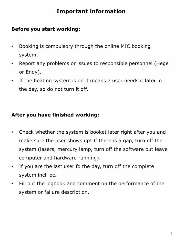
Important information

Before you start working:

• Booking is compulsory through the online MIC booking

system.

• Report any problems or issues to responsible personnel (Hege

or Endy).

• If the heating system is on it means a user needs it later in

the day, so do not turn it off.

After you have finished working:

• Check whether the system is booket later right after you and

make sure the user shows up! If there is a gap, turn off the

system (lasers, mercury lamp, turn off the software but leave

computer and hardware running).

• If you are the last user fo the day, turn off the complete

system incl. pc.

• Fill out the logbook and comment on the performance of the

system or failure description.

3

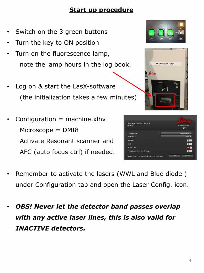
Start up procedure

• Switch on the 3 green buttons

• Turn the key to ON position

• Turn on the fluorescence lamp,

note the lamp hours in the log book.

• Log on & start the LasX-software

(the initialization takes a few minutes)

• Configuration = machine.xlhv

Microscope = DMI8

Activate Resonant scanner and

AFC (auto focus ctrl) if needed.

• Remember to activate the lasers (WWL and Blue diode )

under Configuration tab and open the Laser Config. icon.

• OBS! Never let the detector band passes overlap

with any active laser lines, this is also valid for

INACTIVE detectors.

4

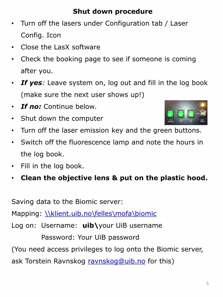
Shut down procedure

• Turn off the lasers under Configuration tab / Laser

Config. Icon

• Close the LasX software

• Check the booking page to see if someone is coming

after you.

• If yes: Leave system on, log out and fill in the log book

(make sure the next user shows up!)

• If no: Continue below.

• Shut down the computer

• Turn off the laser emission key and the green buttons.

• Switch off the fluorescence lamp and note the hours in

the log book.

• Fill in the log book.

• Clean the objective lens & put on the plastic hood.

Saving data to the Biomic server:

Mapping: \\klient.uib.no\felles\mofa\biomic

Log on: Username: uib\your UiB username

Password: Your UiB password

(You need access privileges to log onto the Biomic server,

ask Torstein Ravnskog ravnskog@uib.no for this)

5

6

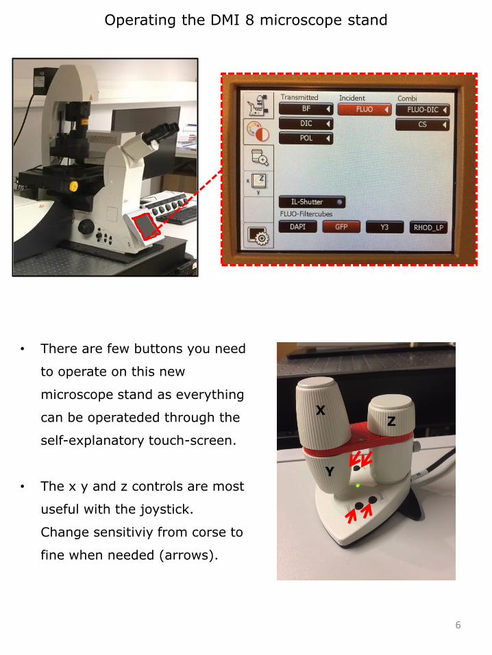
Operating the DMI 8 microscope stand

• There are few buttons you need

to operate on this new

microscope stand as everything

can be operateded through the

self-explanatory touch-screen.

• The x y and z controls are most

useful with the joystick.

Change sensitiviy from corse to

fine when needed (arrows).

Z

Y

X

7

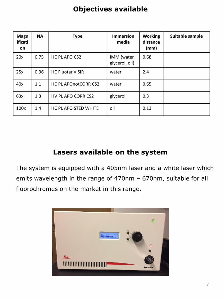
Objectives available

Lasers available on the system

Magnificati

on

NA Type Immersion media

Working distance

(mm)

Suitable sample

20x 0.75 HC PL APO CS2 IMM (water, glycerol, oil)

0.68

25x 0.96 HC Fluotar VISIR water 2.4

40x 1.1 HC PL APOnotCORR CS2 water 0.65

63x 1.3 HV PL APO CORR CS2 glycerol 0.3

100x 1.4 HC PL APO STED WHITE oil 0.13

The system is equipped with a 405nm laser and a white laser which

emits wavelength in the range of 470nm – 670nm, suitable for all

fluorochromes on the market in this range.

8

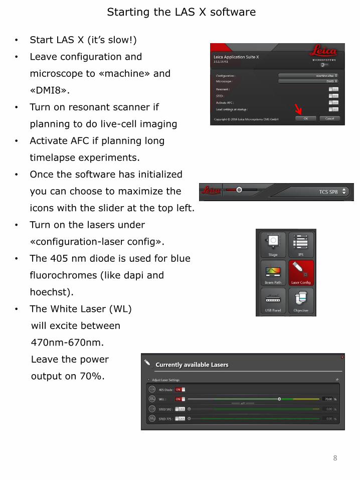
Starting the LAS X software

• Start LAS X (it’s slow!)

• Leave configuration and

microscope to «machine» and

«DMI8».

• Turn on resonant scanner if

planning to do live-cell imaging

• Activate AFC if planning long

timelapse experiments.

• Once the software has initialized

you can choose to maximize the

icons with the slider at the top left.

• Turn on the lasers under

«configuration-laser config».

• The 405 nm diode is used for blue

fluorochromes (like dapi and

hoechst).

• The White Laser (WL)

will excite between

470nm-670nm.

Leave the power

output on 70%.

9

Select the appropiate objective

Magnificati

on

NA Type Immersion media

Working distance

(mm)

Suitable sample

20x 0.75 HC PL APO CS2 IMM (water, glycerol, oil)

0.68

25x 0.96 HC Fluotar VISIR water 2.4

40x 1.1 HC PL APOnotCORR CS2 water 0.65

63x 1.3 HV PL APO CORR CS2 glycerol 0.3

100x 1.4 HC PL APO STED WHITE oil 0.13

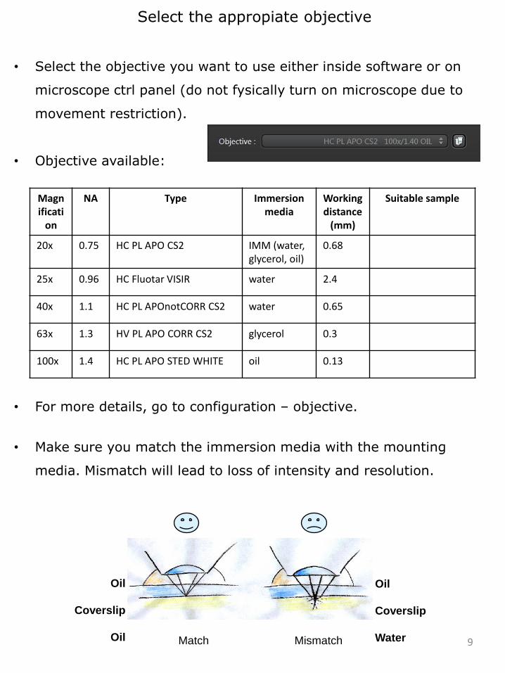
• Select the objective you want to use either inside software or on

microscope ctrl panel (do not fysically turn on microscope due to

movement restriction).

• Objective available:

• For more details, go to configuration – objective.

• Make sure you match the immersion media with the mounting

media. Mismatch will lead to loss of intensity and resolution.

Refractive index mismatch results in spherical aberration

Oil

Coverslip

Water Mismatch Match

Oil

Coverslip

Oil

10

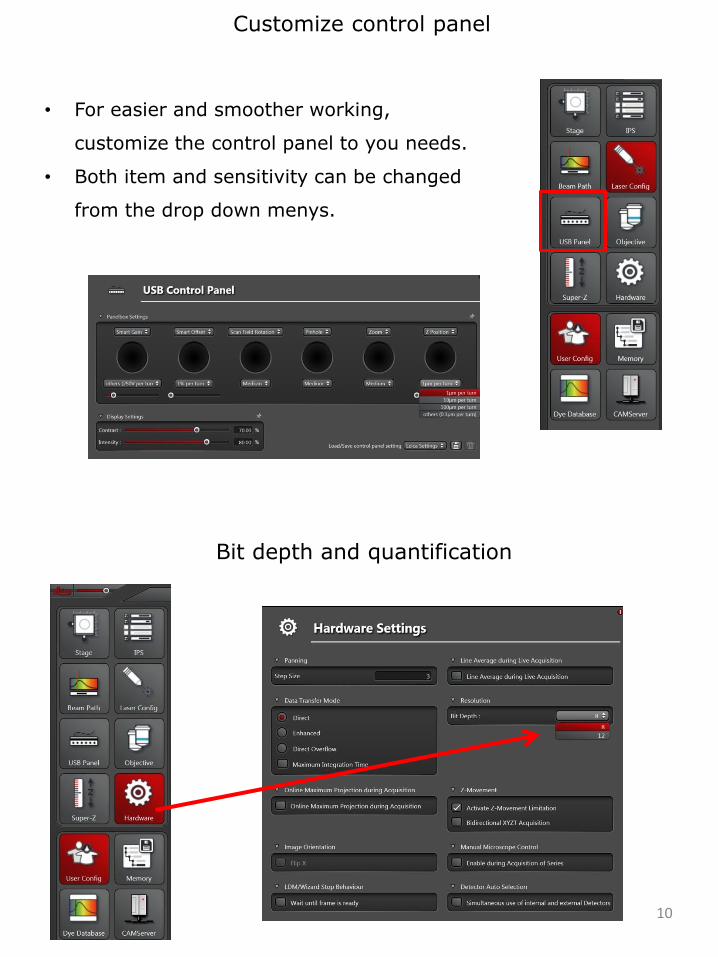
Customize control panel

• For easier and smoother working,

customize the control panel to you needs.

• Both item and sensitivity can be changed

from the drop down menys.

Bit depth and quantification

11

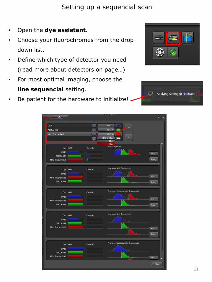
Setting up a sequencial scan

• Open the dye assistant.

• Choose your fluorochromes from the drop

down list.

• Define which type of detector you need

(read more about detectors on page…)

• For most optimal imaging, choose the

line sequencial setting.

• Be patient for the hardware to initialize!

12

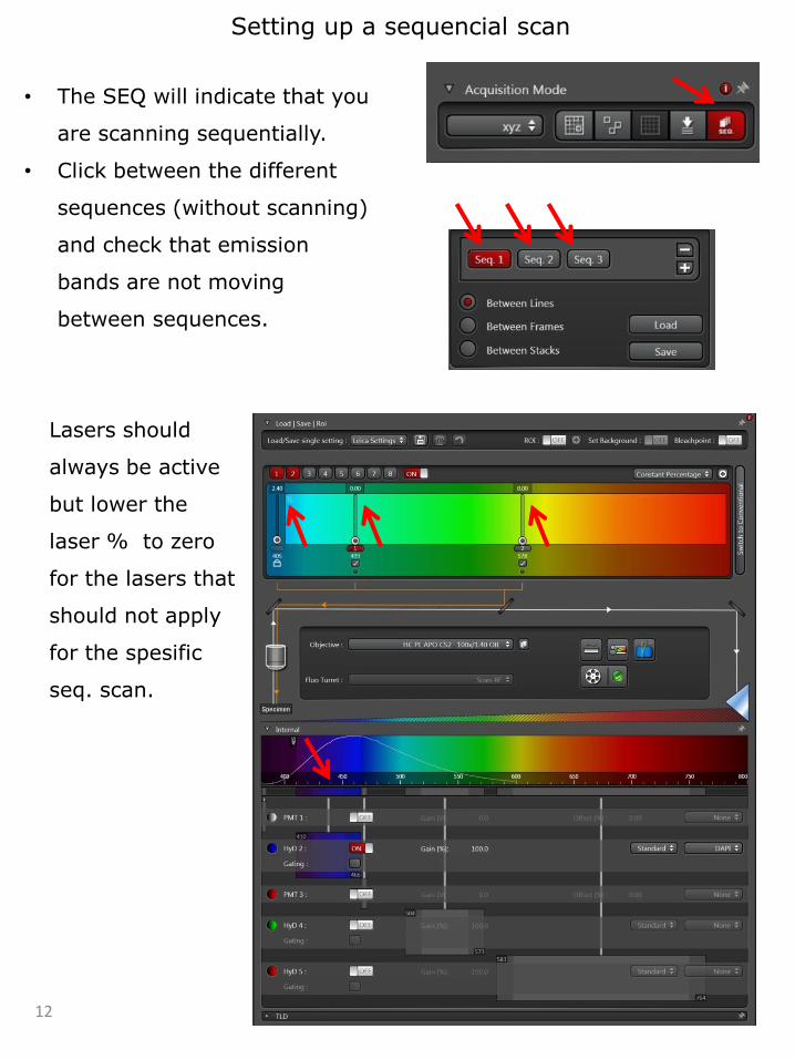
Setting up a sequencial scan

• The SEQ will indicate that you

are scanning sequentially.

• Click between the different

sequences (without scanning)

and check that emission

bands are not moving

between sequences.

Lasers should

always be active

but lower the

laser % to zero

for the lasers that

should not apply

for the spesific

seq. scan.

13

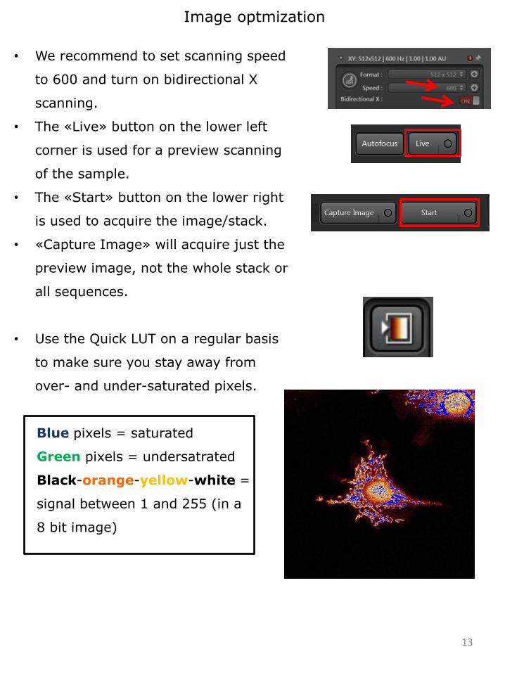
Image optmization

• We recommend to set scanning speed

to 600 and turn on bidirectional X

scanning.

• The «Live» button on the lower left

corner is used for a preview scanning

of the sample.

• The «Start» button on the lower right

is used to acquire the image/stack.

• «Capture Image» will acquire just the

preview image, not the whole stack or

all sequences.

• Use the Quick LUT on a regular basis

to make sure you stay away from

over- and under-saturated pixels.

Blue pixels = saturated

Green pixels = undersatrated

Black-orange-yellow-white =

signal between 1 and 255 (in a

8 bit image)

• Scan speed is measured in Hz (lines per second). It refers to the

frequency of two galvanometers which drive scanning mirrors,

shading laser light across the specimen.

• You can select between 10-1800 Hz on the regular scanner while

the resonant scanner is fixed to 8000 Hz (with min zoom of 1.25).

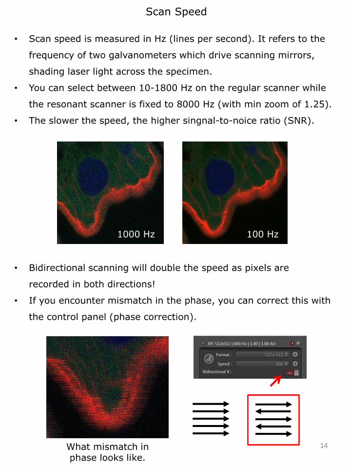
• The slower the speed, the higher singnal-to-noice ratio (SNR).

• Bidirectional scanning will double the speed as pixels are

recorded in both directions!

• If you encounter mismatch in the phase, you can correct this with

the control panel (phase correction).

14

Scan Speed

What mismatch in phase looks like.

1000 Hz 100 Hz

15

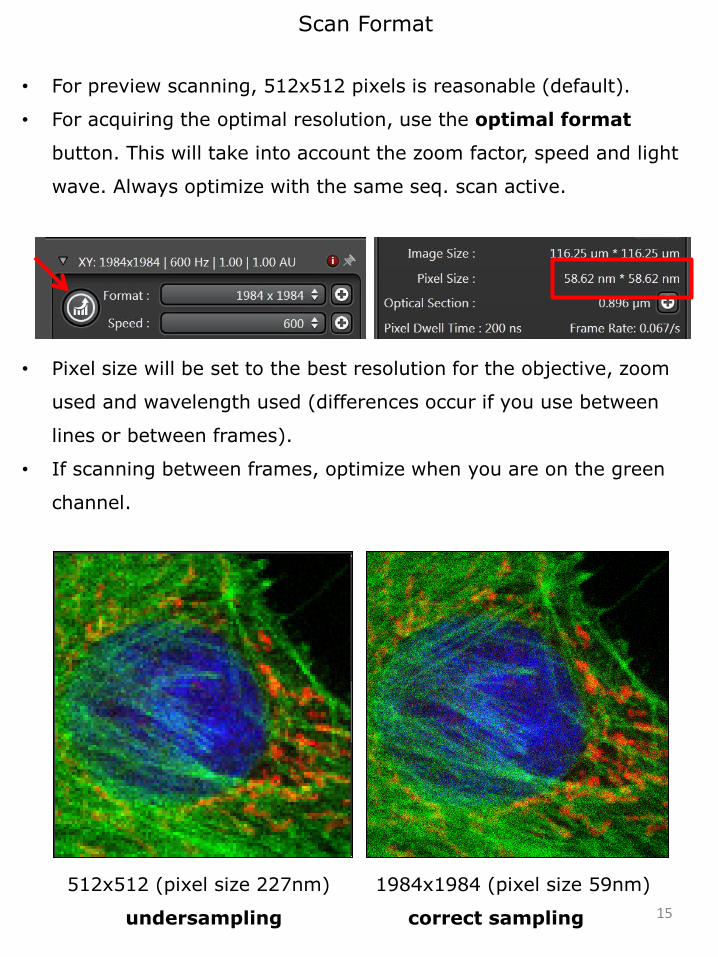
Scan Format

• For preview scanning, 512x512 pixels is reasonable (default).

• For acquiring the optimal resolution, use the optimal format

button. This will take into account the zoom factor, speed and light

wave. Always optimize with the same seq. scan active.

• Pixel size will be set to the best resolution for the objective, zoom

used and wavelength used (differences occur if you use between

lines or between frames).

• If scanning between frames, optimize when you are on the green

channel.

512x512 (pixel size 227nm) 1984x1984 (pixel size 59nm)

undersampling correct sampling

16

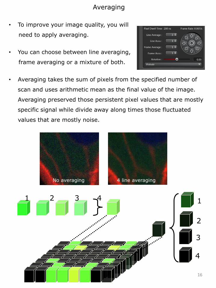
Averaging

• To improve your image quality, you will

need to apply averaging.

• You can choose between line averaging,

frame averaging or a mixture of both.

• Averaging takes the sum of pixels from the specified number of

scan and uses arithmetic mean as the final value of the image.

Averaging preserved those persistent pixel values that are mostly

specific signal while divide away along times those fluctuated

values that are mostly noise.

1

2

3

4

1 2 3 4

No averaging 4 line averaging

17

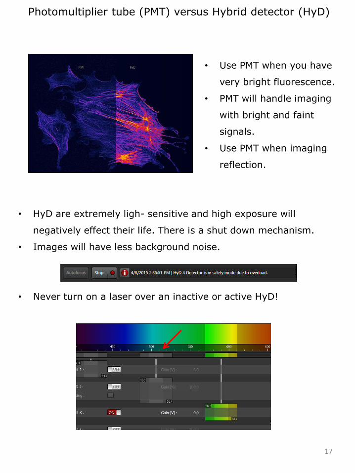
Photomultiplier tube (PMT) versus Hybrid detector (HyD)

• Use PMT when you have

very bright fluorescence.

• PMT will handle imaging

with bright and faint

signals.

• Use PMT when imaging

reflection.

• HyD are extremely ligh- sensitive and high exposure will

negatively effect their life. There is a shut down mechanism.

• Images will have less background noise.

• Never turn on a laser over an inactive or active HyD!

18

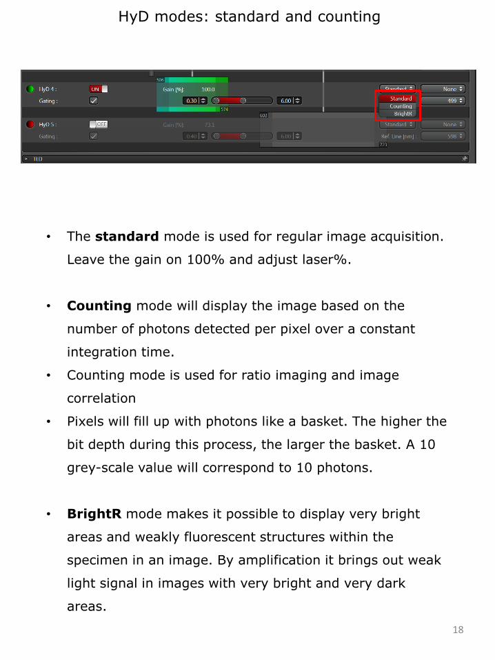
HyD modes: standard and counting

• The standard mode is used for regular image acquisition.

Leave the gain on 100% and adjust laser%.

• Counting mode will display the image based on the

number of photons detected per pixel over a constant

integration time.

• Counting mode is used for ratio imaging and image

correlation

• Pixels will fill up with photons like a basket. The higher the

bit depth during this process, the larger the basket. A 10

grey-scale value will correspond to 10 photons.

• BrightR mode makes it possible to display very bright

areas and weakly fluorescent structures within the

specimen in an image. By amplification it brings out weak

light signal in images with very bright and very dark

areas.

19

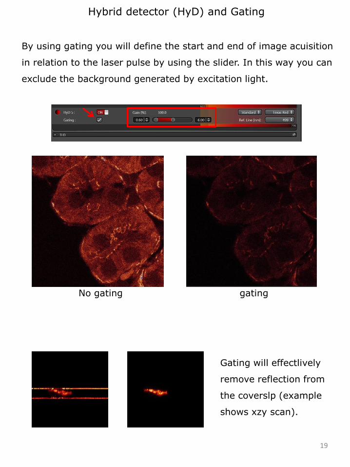
Hybrid detector (HyD) and Gating

By using gating you will define the start and end of image acuisition

in relation to the laser pulse by using the slider. In this way you can

exclude the background generated by excitation light.

No gating gating

Gating will effectlively

remove reflection from

the coverslp (example

shows xzy scan).

20

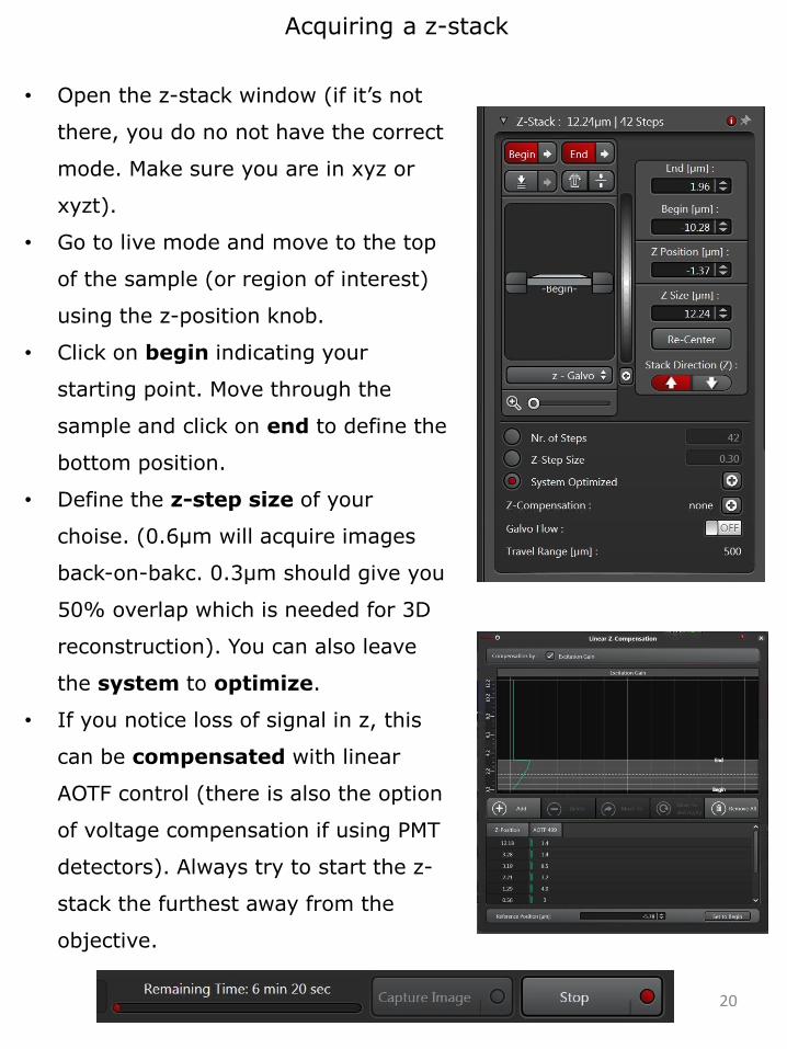
Acquiring a z-stack

• Open the z-stack window (if it’s not

there, you do no not have the correct

mode. Make sure you are in xyz or

xyzt).

• Go to live mode and move to the top

of the sample (or region of interest)

using the z-position knob.

• Click on begin indicating your

starting point. Move through the

sample and click on end to define the

bottom position.

• Define the z-step size of your

choise. (0.6µm will acquire images

back-on-bakc. 0.3µm should give you

50% overlap which is needed for 3D

reconstruction). You can also leave

the system to optimize.

• If you notice loss of signal in z, this

can be compensated with linear

AOTF control (there is also the option

of voltage compensation if using PMT

detectors). Always try to start the z-

stack the furthest away from the

objective.

21

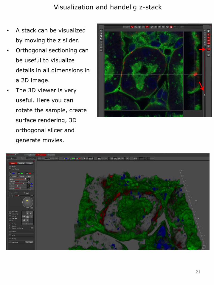
Visualization and handelig z-stack

• A stack can be visualized

by moving the z slider.

• Orthogonal sectioning can

be useful to visualize

details in all dimensions in

a 2D image.

• The 3D viewer is very

useful. Here you can

rotate the sample, create

surface rendering, 3D

orthogonal slicer and

generate movies.

22

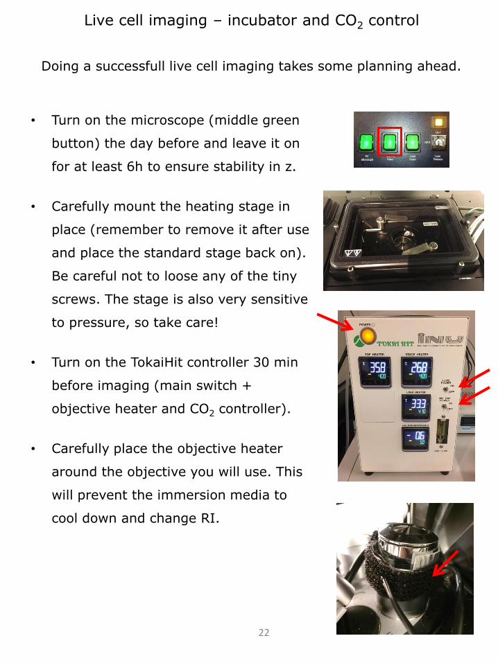
Live cell imaging – incubator and CO2 control

• Turn on the microscope (middle green

button) the day before and leave it on

for at least 6h to ensure stability in z.

• Carefully mount the heating stage in

place (remember to remove it after use

and place the standard stage back on).

Be careful not to loose any of the tiny

screws. The stage is also very sensitive

to pressure, so take care!

• Turn on the TokaiHit controller 30 min

before imaging (main switch +

objective heater and CO2 controller).

• Carefully place the objective heater

around the objective you will use. This

will prevent the immersion media to

cool down and change RI.

Doing a successfull live cell imaging takes some planning ahead.

23

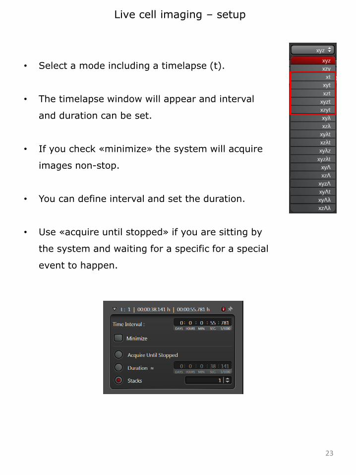
Live cell imaging – setup

• Select a mode including a timelapse (t).

• The timelapse window will appear and interval

and duration can be set.

• If you check «minimize» the system will acquire

images non-stop.

• You can define interval and set the duration.

• Use «acquire until stopped» if you are sitting by

the system and waiting for a specific for a special

event to happen.

24

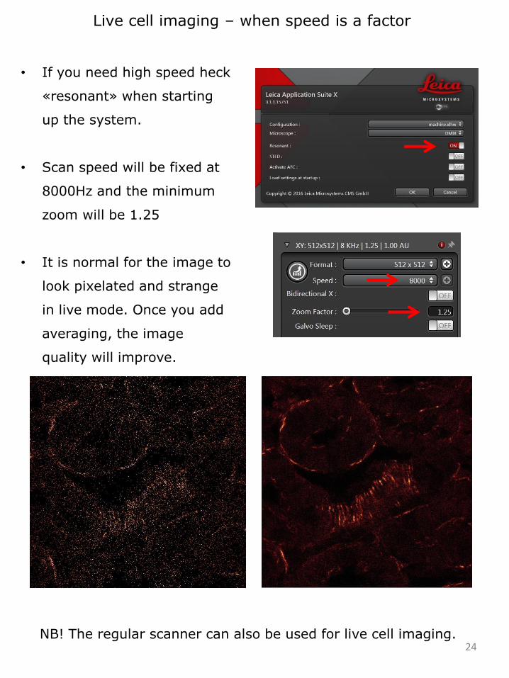
Live cell imaging – when speed is a factor

• If you need high speed heck

«resonant» when starting

up the system.

• Scan speed will be fixed at

8000Hz and the minimum

zoom will be 1.25

• It is normal for the image to

look pixelated and strange

in live mode. Once you add

averaging, the image

quality will improve.

NB! The regular scanner can also be used for live cell imaging.

25

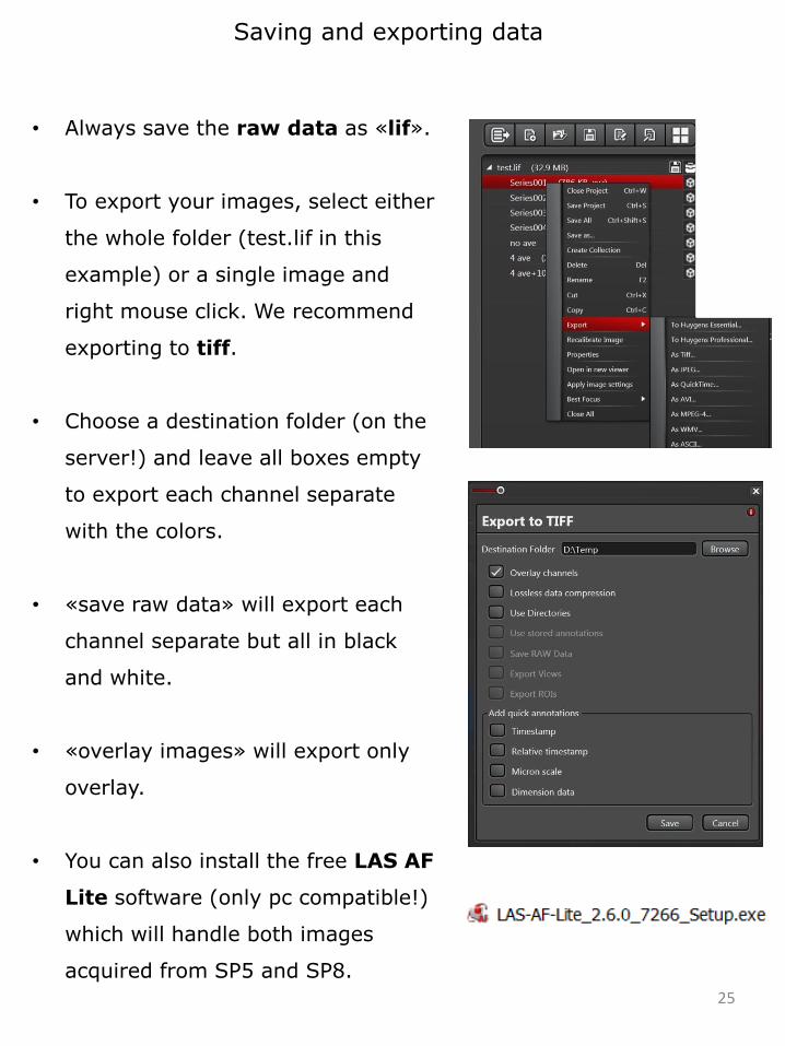
Saving and exporting data

• Always save the raw data as «lif».

• To export your images, select either

the whole folder (test.lif in this

example) or a single image and

right mouse click. We recommend

exporting to tiff.

• Choose a destination folder (on the

server!) and leave all boxes empty

to export each channel separate

with the colors.

• «save raw data» will export each

channel separate but all in black

and white.

• «overlay images» will export only

overlay.

• You can also install the free LAS AF

Lite software (only pc compatible!)

which will handle both images

acquired from SP5 and SP8.

26

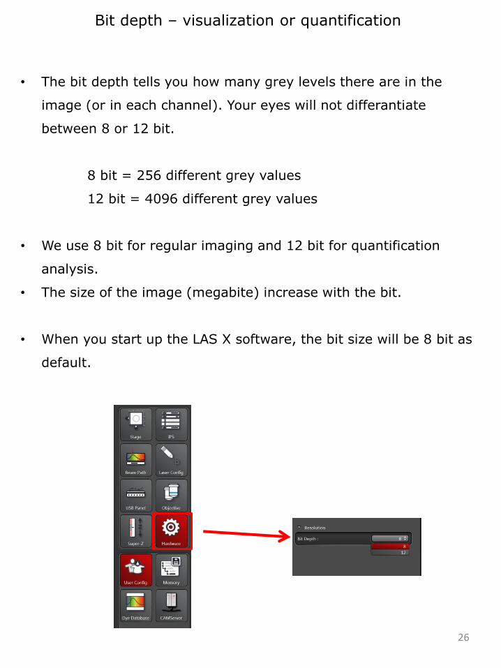
Bit depth – visualization or quantification

• The bit depth tells you how many grey levels there are in the

image (or in each channel). Your eyes will not differantiate

between 8 or 12 bit.

8 bit = 256 different grey values

12 bit = 4096 different grey values

• We use 8 bit for regular imaging and 12 bit for quantification

analysis.

• The size of the image (megabite) increase with the bit.

• When you start up the LAS X software, the bit size will be 8 bit as

default.

27

28

29