User Mobility in IEEE 802.11 Network Environments - Department of
126
IMPERIAL COLLEGE LONDON Department Of Computing User Mobility in IEEE 802.11 Network Environments by Heng Sok Supervisor: Prof. Kin Leung Second Marker: Dr. Paolo Costa A thesis submitted in partial fulfillment of the requirements for the degree of Bachelor of Engineering in Computing June 2013
Transcript of User Mobility in IEEE 802.11 Network Environments - Department of

IMPERIAL COLLEGE LONDON
Department Of Computing
User Mobility in IEEE 802.11
Network Environments
by
Heng SokSupervisor: Prof. Kin Leung
Second Marker: Dr. Paolo Costa
A thesis submitted in partial fulfillment
of the requirements for the degree of
Bachelor of Engineering in Computing
June 2013

“Choose a job that you like, and you will never have to work a day in your life.”
- Confucius

Acknowledgements
First of all, I would like to thank Prof. Kin Leung and Dr. Paolo Costa for their
continual support and advice throughout this project.
Kin has always been there to provide invaluable suggestions and the necessary sup-
port that I need to complete this project successfully. I thank him for sparing his time
for our discussion, especially in one occasion, which took up most of his lunchtime.
He has continuously inspired and motivated me throughout this project. Not only Kin
serves as my supervisor, he also advised me on how to cope with the busy schedule of
university life.
I thank Paolo for sparing his time for our discussions and advising me on how to
improve on the evaluation of my project. He suggested a micro-benchmark experiment,
which serves to test the sensitivity of the detection mechanism used in this project. He
has also advised me on the key points that I need to focus in my report as well as
explaining how a good thesis structure should be.
I also would like to thank Dr. Abdelmalik Bachir for sharing some of his insights and
explain the idea behind the overlapping of WiFi channels. I thank Mr. Duncan White
for supportively helping me to seek permission from ICT Networks and ICT Security to
conduct the experiment in the Department Of Computing Laboratory.
I thank all my friends, especially Arthur, Bolun, Howon, Myung, Yuxiang and
Zhaoyang for helping me out by taking part in the Micro-benchmark Experiment, in
which each of them had to perform various movements in public places. I thank also my
friends who were there to help me look after my equipments during the experiment that
was going on in the laboratory as I had to go out to get lunch on each of the 5 days.
Finally, without my parents and family, I would not be able to achieve what I have
today and complete my education at Imperial. They are my pillars of support throughout
the course of my education, giving me the strength to fight one of the toughest battle
of my life.
ii
Abstract
Understanding the mobility of people within an environment without the aid of
technology is almost impossible due to the fact that it is beyond our ability to remember
all faces of people that appear within that environment and keeping our eyes on their
movement. Even if we ask these people to report about their locations to a central
coordinator every now and then, that would require the use of technology to convey
these messages as well.
We develop a novel system to track the collective mobility of WiFi users within
an environment and instead of a person reporting about his or her location, the WiFi
gadget such as a smartphone that a person carries would inform us about his or her
location and also enabling us to determine how long he or she is staying at a particular
place without his or her knowledge. In this project, we would focus on collective results
to understand a general mobility behaviour of people within one environment rather
than focusing on an individual person. In addition, we demonstrate that our system
could track the collective mobility of WiFi users by putting it to a real test, tracking
the mobility behaviour of the Department Of Computing’s students for 5 days.
iii

Contents
Acknowledgements ii
Abstract iii
List of Figures vii
List of Tables ix
Abbreviations x
1 Introduction 1
1.1 Objectives . . . . . . . . . . . . . . . . . . . . . . . . . . . . . . . . . . . . 3
1.2 Contributions . . . . . . . . . . . . . . . . . . . . . . . . . . . . . . . . . . 3
1.3 Structure of Thesis . . . . . . . . . . . . . . . . . . . . . . . . . . . . . . . 4
2 Background 8
2.1 Understanding IEEE 802.11 standards . . . . . . . . . . . . . . . . . . . . 8
2.1.1 WiFi Channels . . . . . . . . . . . . . . . . . . . . . . . . . . . . . 9
2.1.2 RSSI & SNR . . . . . . . . . . . . . . . . . . . . . . . . . . . . . . 10
2.1.3 Management Frames . . . . . . . . . . . . . . . . . . . . . . . . . . 11
2.1.4 Active versus Passive Scanning . . . . . . . . . . . . . . . . . . . . 12
2.1.5 Joining and Leaving a WLAN . . . . . . . . . . . . . . . . . . . . . 13
2.2 Wireless Chipset and Network Interface Card (NIC) . . . . . . . . . . . . 14
2.2.1 Types of Chipsets . . . . . . . . . . . . . . . . . . . . . . . . . . . 14
2.2.2 List of Broadcom Chipset Commands . . . . . . . . . . . . . . . . 15
2.2.3 NIC modes . . . . . . . . . . . . . . . . . . . . . . . . . . . . . . . 16
2.3 Custom OS for AP . . . . . . . . . . . . . . . . . . . . . . . . . . . . . . . 16
2.3.1 DD-WRT . . . . . . . . . . . . . . . . . . . . . . . . . . . . . . . . 16
2.3.2 OpenWrt . . . . . . . . . . . . . . . . . . . . . . . . . . . . . . . . 17
2.4 Related Wireless LAN Software tools . . . . . . . . . . . . . . . . . . . . . 18
2.4.1 Kismet . . . . . . . . . . . . . . . . . . . . . . . . . . . . . . . . . 18
2.4.2 NetStumbler . . . . . . . . . . . . . . . . . . . . . . . . . . . . . . 18
2.4.3 Wireshark . . . . . . . . . . . . . . . . . . . . . . . . . . . . . . . . 19
2.4.4 Wiviz . . . . . . . . . . . . . . . . . . . . . . . . . . . . . . . . . . 19
2.4.5 Tcpdump and libpcap . . . . . . . . . . . . . . . . . . . . . . . . . 19
2.4.6 Summary . . . . . . . . . . . . . . . . . . . . . . . . . . . . . . . . 20
2.5 Data Transmission . . . . . . . . . . . . . . . . . . . . . . . . . . . . . . . 20
2.5.1 Serialisation of Data . . . . . . . . . . . . . . . . . . . . . . . . . . 20
2.5.2 File Transfer Library for Embedded Devices . . . . . . . . . . . . . 21
2.6 Storing and Aggregating Big Data . . . . . . . . . . . . . . . . . . . . . . 22
2.6.1 Relational SQL versus NoSQL database . . . . . . . . . . . . . . . 22
iv

Contents
2.6.2 NoSQL Databases . . . . . . . . . . . . . . . . . . . . . . . . . . . 23
2.6.3 MapReduce Framework . . . . . . . . . . . . . . . . . . . . . . . . 25
2.7 Summary . . . . . . . . . . . . . . . . . . . . . . . . . . . . . . . . . . . . 27
3 Related Work 29
3.1 Mechanisms for Tracking WiFi Terminals . . . . . . . . . . . . . . . . . . 29
3.2 Factors Affecting Accuracy of Detecting WiFi Terminals . . . . . . . . . . 31
3.3 Localisation Techniques . . . . . . . . . . . . . . . . . . . . . . . . . . . . 32
3.4 Summary . . . . . . . . . . . . . . . . . . . . . . . . . . . . . . . . . . . . 32
4 Design 33
4.1 Overview of Design Architecture . . . . . . . . . . . . . . . . . . . . . . . 33
4.2 Detection Mechanisms . . . . . . . . . . . . . . . . . . . . . . . . . . . . . 36
4.3 Types of Aggregation . . . . . . . . . . . . . . . . . . . . . . . . . . . . . 39
4.4 Web GUI . . . . . . . . . . . . . . . . . . . . . . . . . . . . . . . . . . . . 39
5 Implementation 40
5.1 Chipset and Custom AP Firmware . . . . . . . . . . . . . . . . . . . . . . 40
5.1.1 Choosing a Suitable Firmware . . . . . . . . . . . . . . . . . . . . 41
5.1.2 Preparing Firmware . . . . . . . . . . . . . . . . . . . . . . . . . . 42
5.1.3 Flashing AP Filesystem . . . . . . . . . . . . . . . . . . . . . . . . 43
5.2 Detecting, Transferring and Compiling . . . . . . . . . . . . . . . . . . . . 44
5.2.1 Detection Program . . . . . . . . . . . . . . . . . . . . . . . . . . . 44
5.2.2 Data Serialisation . . . . . . . . . . . . . . . . . . . . . . . . . . . 48
5.2.3 Securing Transmission . . . . . . . . . . . . . . . . . . . . . . . . . 50
5.2.4 File Transmission . . . . . . . . . . . . . . . . . . . . . . . . . . . . 50
5.2.5 Cross Compiling Program . . . . . . . . . . . . . . . . . . . . . . . 53
5.3 Building a Processing Agent . . . . . . . . . . . . . . . . . . . . . . . . . . 56
5.3.1 Initialising Web Servlet . . . . . . . . . . . . . . . . . . . . . . . . 56
5.3.2 Receiving and Deserialising Data . . . . . . . . . . . . . . . . . . . 56
5.3.3 Adding Timestamp . . . . . . . . . . . . . . . . . . . . . . . . . . . 57
5.3.4 Pushing Data to Database . . . . . . . . . . . . . . . . . . . . . . . 59
5.4 Storing and Managing Data . . . . . . . . . . . . . . . . . . . . . . . . . . 59
5.4.1 Comparison between HBase and CouchDB . . . . . . . . . . . . . 60
5.4.2 Setting up of HBase, HDFS, MapReduce and Zookeeper . . . . . . 62
5.4.3 Data Schema Design . . . . . . . . . . . . . . . . . . . . . . . . . . 63
5.5 Aggregating Data . . . . . . . . . . . . . . . . . . . . . . . . . . . . . . . . 66
5.5.1 Overview of Aggregation Process . . . . . . . . . . . . . . . . . . . 67
5.5.2 Localising Terminals . . . . . . . . . . . . . . . . . . . . . . . . . . 68
5.5.3 Count Statistics . . . . . . . . . . . . . . . . . . . . . . . . . . . . 71
5.5.4 Residence Time . . . . . . . . . . . . . . . . . . . . . . . . . . . . . 74
5.5.5 New Versus Returning . . . . . . . . . . . . . . . . . . . . . . . . . 77
5.5.6 Summary . . . . . . . . . . . . . . . . . . . . . . . . . . . . . . . . 79
v
Contents
5.6 GUI Design and Implementation . . . . . . . . . . . . . . . . . . . . . . . 80
5.6.1 Retrieving Data from HBase . . . . . . . . . . . . . . . . . . . . . 81
5.6.2 Making Asychronous Ajax Request . . . . . . . . . . . . . . . . . . 84
5.6.3 CountLive and CountStatistics . . . . . . . . . . . . . . . . . . . . 85
5.6.4 ResidenceTime and ResidenceTime Overall . . . . . . . . . . . . . 87
5.6.5 New and Returning Visitors . . . . . . . . . . . . . . . . . . . . . . 87
6 Evaluation 89
6.1 Setting up of Experiment in Laboratory . . . . . . . . . . . . . . . . . . . 89
6.1.1 Deployment Overview . . . . . . . . . . . . . . . . . . . . . . . . . 90
6.1.2 Monitoring APs’ Heartbeat . . . . . . . . . . . . . . . . . . . . . . 91
6.2 Measuring Performance of Terminals Detection . . . . . . . . . . . . . . . 92
6.2.1 Procedure to Prepare Evaluation Graphs . . . . . . . . . . . . . . 92
6.2.2 Factors Affecting Accuracy of Detection . . . . . . . . . . . . . . . 94
6.2.3 Discussion of Results . . . . . . . . . . . . . . . . . . . . . . . . . . 95
6.2.4 Analysing Trends from Web GUI . . . . . . . . . . . . . . . . . . . 99
6.3 Frequency of Probe Request Frames . . . . . . . . . . . . . . . . . . . . . 99
6.3.1 Compiling Process . . . . . . . . . . . . . . . . . . . . . . . . . . . 100
6.3.2 Discussion of Results . . . . . . . . . . . . . . . . . . . . . . . . . . 101
6.4 Microbenchmark . . . . . . . . . . . . . . . . . . . . . . . . . . . . . . . . 102
6.5 Unit Tests . . . . . . . . . . . . . . . . . . . . . . . . . . . . . . . . . . . . 105
6.6 Summary . . . . . . . . . . . . . . . . . . . . . . . . . . . . . . . . . . . . 106
7 Conclusion and Future Extensions 107
7.1 Conclusion . . . . . . . . . . . . . . . . . . . . . . . . . . . . . . . . . . . 107
7.2 Future Extensions . . . . . . . . . . . . . . . . . . . . . . . . . . . . . . . 108
7.2.1 A More Reliable Way of Localising Terminal . . . . . . . . . . . . 108
7.2.2 Enclosing the Environment Under Monitored . . . . . . . . . . . . 109
7.2.3 Ignoring Static Terminals . . . . . . . . . . . . . . . . . . . . . . . 109
7.2.4 Protecting Privacy of Individuals . . . . . . . . . . . . . . . . . . . 109
A Evaluation Tables 110
Bibliography 113
vi
List of Figures
1.1 Illustrating the whole journey we are going to embark on . . . . . . . . . 7
2.1 Representation of WiFi channels overlapping . . . . . . . . . . . . . . . . 10
2.2 Illustration of how MapReduce works . . . . . . . . . . . . . . . . . . . . . 26
4.1 Overview of our deployment strategy . . . . . . . . . . . . . . . . . . . . . 33
4.2 Detecting presence of terminals using probe request . . . . . . . . . . . . 37
5.1 Top level filesystem of firmware image . . . . . . . . . . . . . . . . . . . . 42
5.2 Root filesystem of firmware image . . . . . . . . . . . . . . . . . . . . . . 43
5.3 General IEEE 802.11 frame with Frame Control field highlighted . . . . . 46
5.4 List of all toolchains provided by DD-WRT for cross compiling . . . . . . 53
5.5 The Cross Compiling process . . . . . . . . . . . . . . . . . . . . . . . . . 55
5.6 Detail of the generated executable binary program file . . . . . . . . . . . 55
5.7 Illustration of Documents in CouchDB . . . . . . . . . . . . . . . . . . . . 60
5.8 Storage size for 12817 Documents in CouchDB . . . . . . . . . . . . . . . 61
5.9 Storage size for 5181 rows in HBase . . . . . . . . . . . . . . . . . . . . . 61
5.10 Balance between sequential read and write performance . . . . . . . . . . 64
5.11 MapReduce work flow . . . . . . . . . . . . . . . . . . . . . . . . . . . . . 68
5.12 Structure of Counts of Terminals table . . . . . . . . . . . . . . . . . . . . 73
5.13 Part of the traces of a terminal’s presence across the day . . . . . . . . . . 75
5.14 Structure of Residence Time table . . . . . . . . . . . . . . . . . . . . . . 77
5.15 Structure of History Lookup table . . . . . . . . . . . . . . . . . . . . . . . 78
5.16 Dashboard of our Web GUI . . . . . . . . . . . . . . . . . . . . . . . . . . 80
5.17 Two proposed ways of retrieving data from HBase to Web GUI . . . . . . 81
5.18 Illustration of returned query from HBase REST API . . . . . . . . . . . 84
5.19 Illustration of CountLive page in Web GUI . . . . . . . . . . . . . . . . . 85
5.20 Illustration of histogram on CountStatistics page in Web GUI . . . . . . . 86
5.21 Illustration of Daily View with controller on CountStatistics page in WebGUI . . . . . . . . . . . . . . . . . . . . . . . . . . . . . . . . . . . . . . . 87
5.22 Illustration of ResidenceTime page in Web GUI . . . . . . . . . . . . . . . 88
5.23 Illustration of New and Returning Visitors page in Web GUI . . . . . . . 88
6.1 Overview of deployment . . . . . . . . . . . . . . . . . . . . . . . . . . . . 91
6.2 Monitoring progress of experiment . . . . . . . . . . . . . . . . . . . . . . 92
6.3 Evaluation Table showing details of number of terminals detected andstudents observed . . . . . . . . . . . . . . . . . . . . . . . . . . . . . . . . 93
6.4 Comparing number of terminals being detected and observed near AP3and AP5 on 29/05/2013 filtering out RSSI less than -80 . . . . . . . . . . 96
6.5 Comparing number of terminals being detected and observed near AP3and AP5 on 30/05/2013 filtering out RSSI less than -80 . . . . . . . . . . 97
6.6 Comparing number of terminals being detected and observed near AP3and AP5 on 31/05/2013 filtering out RSSI less than -70 . . . . . . . . . . 97
vii
List of Figures
6.7 Comparing number of terminals being detected and observed near AP3and AP5 on 01/06/2013 filtering out RSSI less than -65 . . . . . . . . . . 98
6.8 Comparing number of terminals being detected and observed near AP3and AP5 on 03/06/2013 filtering out RSSI less than -60 . . . . . . . . . . 98
6.9 Trend of number of students in laboratory . . . . . . . . . . . . . . . . . . 99
6.10 Calculations of probe request frequency . . . . . . . . . . . . . . . . . . . 100
6.11 Probe request frequency of major brands . . . . . . . . . . . . . . . . . . . 101
6.12 Illustration of how students move in Mobility experiment . . . . . . . . . 102
6.13 Number of terminals out of 10 detected in Lab (Static) . . . . . . . . . . . 103
6.14 Number of terminals out of 10 detected in Open Space (Static) . . . . . . 104
6.15 Number of terminals out of 10 detected in Lab (Mobility) . . . . . . . . . 104
6.16 Number of terminals out of 10 detected in Open Space (Mobility) . . . . . 105
6.17 Unit Test showing a test with error . . . . . . . . . . . . . . . . . . . . . . 105
6.18 Unit Test showing a successful test . . . . . . . . . . . . . . . . . . . . . . 106
A.1 Evaluation tables for experiments on 29/05/2013 and 30/05/2013 . . . . . 110
A.2 Evaluation tables for experiments on 31/05/2013 and 01/06/2013 . . . . . 111
A.3 Evaluation tables for experiments on 03/06/2013 . . . . . . . . . . . . . . 112
viii
List of Tables
2.1 Maximum Power Levels Per Antenna Gain for IEEE 802.11b . . . . . . . 9
2.2 IEEE 802.11 Channels . . . . . . . . . . . . . . . . . . . . . . . . . . . . . 10
2.3 Type of Management Frames . . . . . . . . . . . . . . . . . . . . . . . . . 12
2.4 Specification of an AP . . . . . . . . . . . . . . . . . . . . . . . . . . . . . 15
2.5 List of Broadcom chipset Commands . . . . . . . . . . . . . . . . . . . . . 15
2.6 An Example HBase Table Structure . . . . . . . . . . . . . . . . . . . . . 23
5.1 A Record . . . . . . . . . . . . . . . . . . . . . . . . . . . . . . . . . . . . 59
5.2 HBase Table Structure for Detection Records . . . . . . . . . . . . . . . . 63
5.3 A Row Representing a Detection Record in Raw Records table and Lo-calised Terminal Records table . . . . . . . . . . . . . . . . . . . . . . . . 69
5.4 Count Statistics Map Function Output Key and Value . . . . . . . . . . . 72
5.5 Residence Time Map Function Output Key and Value . . . . . . . . . . . 74
ix

Abbreviations
AP Access Point
API Application Programming Interface
GPS Global Positioning System
GUI Graphic User Interface
HDFS Hadoop Distributed File System
IEEE Institute of Electrical and Electronics Engineers
IDL Interface Definition Language
JFFS Journalling Flash File System
MAC Medium Access Control
NIC Network Interface Card
REST REpresentational State Transfer
RSSI Received Signal Strength Indicator
SSID Service Set IDentifier
WLAN Wireless Local Area Network
x
Chapter 1
Introduction
The internet today has evolved rapidly and it looks so different in various aspects
when comparing to how it is like a decade ago. The speed of communication has signifi-
cantly increased, advancing from 56 kbit/s Dial-up connection to the current high-speed
broadband that can reach even more than 100 mbits/s. Another notable aspect of dif-
ference is the rapid improvement in wireless technology such as that defined by the
Institute of Electrical and Electronics Engineers (IEEE) 802.11 standard. Slowly, every
single piece of device around us starts to support this standard and the name WiFi is
given to any products that conform to the IEEE 802.11 standards.
The initial IEEE 802.11 standard was released in 1997 and over the years, there
are new protocols introduced as part of the standard. These include 802.11a, 802.11b,
802.11g, 802.11n and 802.11ac. As newer protocols are being introduced, so does the
improvement in the data rate per stream that this wireless technology support. There
are two main entities that are part of the IEEE 802.11 standard, namely the client and
the base station. The latter can also be referred to as Access Point (AP).
Due to the higher data transfer throughput and robustness of WiFi technology,
popularity of the use of WiFi has increased exponentially over the years as more and
more technological gadgets are produced such as smartphones, tablets, portable gaming
consoles and MP3 players.
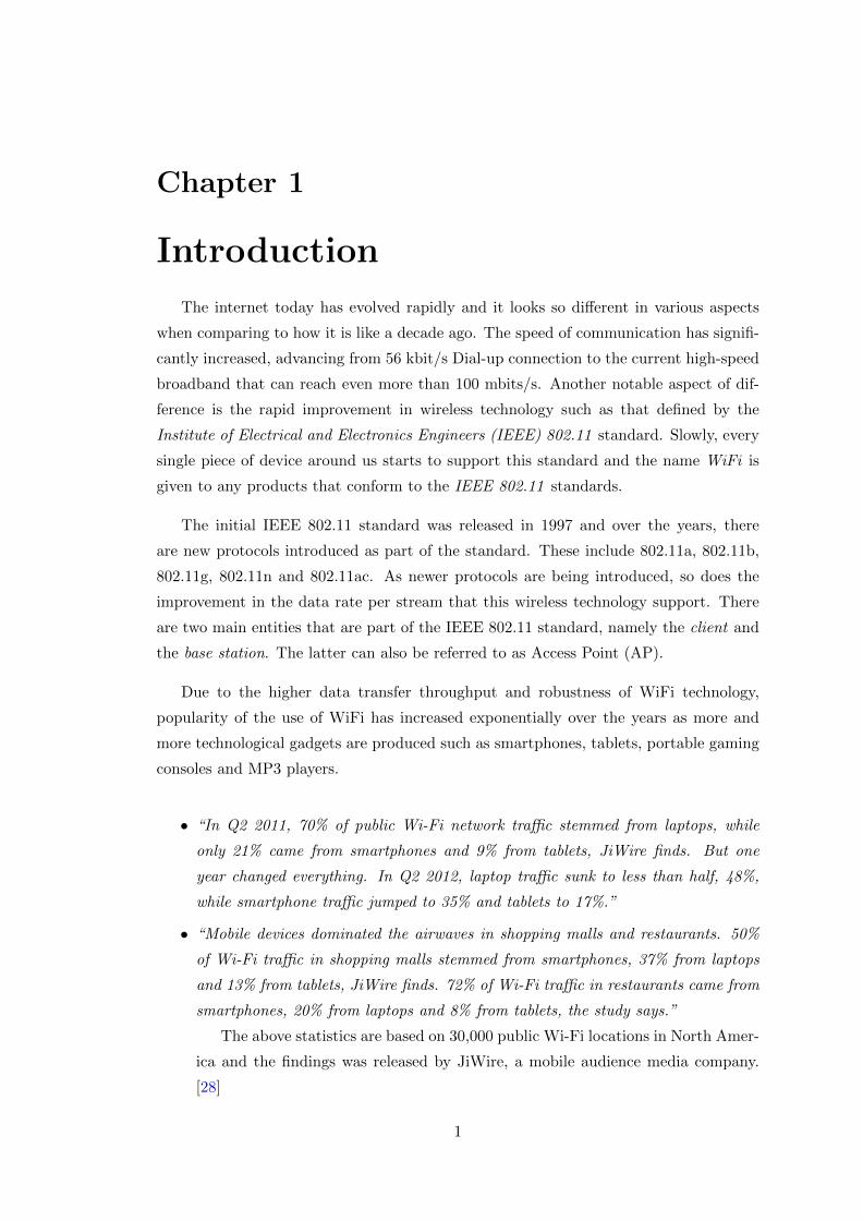
• “In Q2 2011, 70% of public Wi-Fi network traffic stemmed from laptops, while
only 21% came from smartphones and 9% from tablets, JiWire finds. But one
year changed everything. In Q2 2012, laptop traffic sunk to less than half, 48%,
while smartphone traffic jumped to 35% and tablets to 17%.”
• “Mobile devices dominated the airwaves in shopping malls and restaurants. 50%
of Wi-Fi traffic in shopping malls stemmed from smartphones, 37% from laptops
and 13% from tablets, JiWire finds. 72% of Wi-Fi traffic in restaurants came from
smartphones, 20% from laptops and 8% from tablets, the study says.”
The above statistics are based on 30,000 public Wi-Fi locations in North Amer-
ica and the findings was released by JiWire, a mobile audience media company.
[28]
1

Chapter 1. Introduction
By infering from the facts above, we could see that the rise in the number of users
utilising mobile devices to access WiFi network creates a new dimension of opportunities
to exploit this trend especially when APs continue to be widely deployed to accommodate
this rise in usage. The rise in the number of users carrying mobile WiFi devices around
shopping malls and restaurants indicates that it would be really useful for business
owners to learn about the behaviour of these users in their stores. With the large
number of WiFi users, this is the right time to look for ways to harness the potential
and functionalities of WiFi. Since it is also possible to identify devices that have network
connectivity by finding out the globally unique network interface identifier called MAC
address, this opens up a new prospect of localising WiFi-enabled devices. We could
look for a mechanism to localise these users by investigating into how the whole IEEE
802.11 framework works. We could then associate the identification of such devices to
the persons carrying them.
As we start to think about localisation, we may begin to relate the similarity to
the functionalities of GPS, an outdoor navigation system using multiple satellites for
localisation of a GPS-enabled device. Currently, outdoor localisation using GPS is quite
robust. In contrast, indoor localisation is still a problem that needs to be addressed
1. For this reason, coupled with the rise in the popularity of WiFi, it creates a huge
motivation behind this project, in which we aim to understand how devices and network
components under the umbrella of IEEE 802.11 standards interact and function so as to
come up with a solution to detect the presence of users carrying WiFi devices. It would
be more accurate to associate the presence of a user to the detection of a smaller mobile
WiFi devices such as smartphones, in which users tend to carry with them everywhere,
than a WiFi-enabled laptop.
Intuitively, we aim to detect the presence of users carrying WiFi terminals2 without
requiring them to perform any actions. Most of the readily available softwares that are
related to sniffing network traffic usually requires that a terminal already belong to a
network after authentication and association to the relevant AP in the network. What
we want to have is a way to “quietly” detect the presence of a terminal, i.e., passive
detection. This is because it would be extremely hard to persuade users in a public
area to connect to an AP so that useful information about them could be obtained. In
addition, we are interested in analysing the collective mobility behaviour of all users in
1It should be noted that WiFi network may also be deployed outdoor and not necessarily only indooralthough they tend to be widely deployed indoor. Hence, we do not constraint the localisation of usersusing WiFi for indoor only.
2In this project, we consider 802.11 wireless network operating in the infrastructure mode, where asurface area would have at least one defined AP. WiFi terminals surrounding the AP would communicatewith the AP and there is no direct terminal to terminal communications.
2
Chapter 1. Introduction
the environment we are monitoring rather than a specific user’s behaviour. This creates
a challenge to investigate into a way to achieve the aims we want above.
1.1 Objectives
In this project, we would focus on the mechanism to detect WiFi-enabled devices
and use information such as Received Signal Strength Indicator(RSSI) (Section 2.1.2)
to localise these devices, indirectly the users carrying them. We also aim to come up
with an infrastructure design and protocols to facilitate the tracking and analysing of
collective mobility of users in an environment that has WiFi APs deployed. This would
allow us to yield useful statistics such as the time duration that most users spend at
a particular area and the number of users staying at that area. This requires constant
tracking of WiFi users within the environment, in which we have deployed the APs
we have configured to carry out the job. In addition, we come up with the logic and
algorithms to aggregate the data collectively, determining which AP out of all nearby
APs a particular user is closer in proximity. We also aggregate the aggregated data3 to
derive other useful statistics. Lastly, we would provide an interactive web Graphic User
Interface (GUI) that displays the aggregated data, showing appropriate graphs to aid
the understanding of the collected data.
1.2 Contributions
Firstly, we make use of existing tools and libraries to implement a way to detect the
presence of WiFi terminals from an AP. Since this requires access to the AP’s Operating
System (OS), it is not possible to work on the original OS shipped with the AP. In
this project, we use readily available router in the market, which serves as an AP for
detecting the presence of terminals. Since a router is an embedded device that usually
runs on MIPS architecture, this means that we need to compile a program in a different
manner using appropriate toolchain.
Secondly, we design and set up a robust infrastructure for collecting and aggregating
data that scales easily even for large commercial deployment. This touches the topic of
big data since there is always a continuous stream of data from all APs and overtime,
the accumulated data could be very huge in size. All APs sends data about nearby WiFi
terminals in a regular time interval to a central processing agent, which serves to fetch
3Data can be aggregated in many different ways to generate a different representation of the userbehaviour in the network environment.
3

Chapter 1. Introduction
and interpret the data using a chosen serialisation scheme and insert it to the database
for aggregation after that.
Thirdly, We devise the best possible approach to aggregate the collected information
about WiFi terminals that are close to the APs that we deploy. A terminal could be
detected by several APs simultaneously, hence, we need to come up with a way to work
out which AP is closer to the terminal. Other statistical information could also be
drawn from the information collected from all APs to derive an overall view of what
is happening in the environment under monitored. In particular, we are interested in
knowing the number of WiFi users4 staying near each of the AP, the duration of time
they stay and the number of users who return to a location near the AP that they have
come across before.
Fourthly, we design a user-friendly GUI that could be used by business owners or
administrators for displaying the aggregated results so as to make sense out of the
numerical data. Histogram, piechart and a simple probability density distribution are
drawn up to aid the understanding of statistical data. In order to accomplish the goal
of querying data straight away in Javascript from HBase (Section 2.6.2), a database
we choose for this project, we write code for a REST API wrapper and a Javascript
Bytes Utility for HBase5, which are currently not available for HBase. We release these
utilities to the HBase community under Apache License Version 2.0. Majority of the
Web GUI is extensively written in Javascript since this creates an “app-like” effect such
that browser users do not need to refresh the page after selecting some options on the
browser screen. This requires making many asynchronous calls and proper handling of
the returned results.
Finally, we carry out a lab-wide experiment in the Department Of Computing Labo-
ratory and Common room to test the effectiveness and accuracy of detecting the number
of WiFi users in the vicinity and their behaviour in the tested environment.
1.3 Structure of Thesis
In this project, we propose various mechanisms to detect the presence of WiFi ter-
minals and one of the best methods is implemented. Since there is a possibility that
this project could be extended to study the mobility of users in a larger area or be used
in a commercial roll-out that consists of many APs in various locations, we keep this in
4We may sometimes refer to WiFi users being a user who carries a WiFi terminal such as a smartphoneor a tablet.
5The Byte Utility allows the conversion of data types from bytes array that are stored in HBase tableto Integer, Long, Short and String data types directly in Javascript.
4

Chapter 1. Introduction
mind while designing our whole ecosystem. Other than just detecting the presence of
terminals, we also define a message transfer protocols, in which data collected at each
AP could be sent to a central server for processing. An appropriate database technology
would be considered in conjunction with the way we need to aggregate the data collected
from each AP. We choose the current most efficient way of aggregating big data, for large
deployment of many APs, and also a database technology that can scale to petabytes in
size.
In Chapter 2, we dive into the technical details that are relevant for understanding
and implementing a working prototype for tracking user mobility. We examine and
decide on an appropriate open source OS for APs that we would use in our prototype.
We consider the functionalities, code libraries, stability and level of support for the OS
before making our decision. We also discuss the current major chipset manufacturer for
APs since we need to decide on one chipset for implementation. Different chipsets could
be built based on different computer architecture, such as ARM or MIPS, hence there are
different code libraries available. Thus, we can only focus on one chipset in this project.
We can tap into the available open source libraries to our advantage. Furthermore, we
also evaluate different database technology to select an appropriate one for our project.
We continue to discuss about related work in the field of our project in Chapter
3. A few different mechanisms are employed by different papers to track user mobility,
with emphasis on different localisation techniques that aims to locate a WiFi user as
accurately as possible. Although we do not focus on high accuracy of localising a user
in this project, it would still be useful to understand these localisation algorithms so
that we are aware of the different ways of solving the limitations that we observe in this
project. Since we use only RSSI information to determine whether a WiFi terminal is
closer to a particular AP or another, this leads to issue such as the “Ping Pong” effect6,
which is a phenomenon that we have observed after conducting the experiment in the
laboratory.
Chapter 4 presents a simplistic view of the overall architecture of how we go about
tracking WiFi terminals, managing the data and processing it, as well as storing the
aggregated results for displaying on a GUI. Different server components are discussed
to give an idea of how each component works together to achieve the aim of obtaining
a statistical view of user mobility in general.
In Chapter 5, we explain the details behind our implementation, presenting different
technical viewpoints and difficulties. We also give the rationale behind each of the
6“Ping Pong” effect usually happens when the received signal strength becomes unreliable at timesleading to a WiFi terminal being associated with one AP at one time and to another at subsequent timealthough the terminal has not moved. This effect is most commonly observed when a terminal is locateddirectly in between two APs.
5
Chapter 1. Introduction
decisions that we have make for selecting a suitable solution to solve each of the sub-
problems, which are essential to build an overall working implementation for tracking
collective mobility of users. The implementation has been designed to have the ability
to scale easily and flexibly.
There are 3 main phases we need to focus on,
• Mechanism to detect the presence of terminals
• Aggregating data
• Generating graphs and displaying the results via a Web GUI
Chapter 6 details the evaluation process, in which we have conducted a variety of
experiments to evaluate the performance of our system. We have also written some unit
tests to verify the correctness of our algorithms. We give these details below:
1. We deployed 6 APs in the Department Of Computing (DOC) Laboratory and
Common room to track the mobility behaviour of DOC students and staffs. Ob-
servations of the actual environment were make to evaluate the efficiency and
accuracy of our system in tracking users in the environment where our APs were
deployed.
2. We conducted a micro-benchmark experiment. This experiment involves a group
of students, each carrying two WiFi terminals with them and they are supposed
to stay at different intervals of distance from an AP so that we could determine
how many of them we could still detect as they move together as a group away
from the AP.
3. We process the raw data collected from the experiment in the laboratory and we
take sample of the population of WiFi terminals to determine the frequency of
probe request being sent out by the different brand of terminals. (Section 2.1.4)
Examples of brand includes Samsung, Apple, LG, Research In Motion and others.
It is essential to know this information to verify the accuracy of the mechanism
that we have used in our implementation which we would elaborate in Chapter
(5).
4. Aggregating the collected data requires understanding what the data means so as
to verify that the logic in place for the aggregation is working as expected. This
involves printing out the information at each step of the algorithm to check its
correctness and some unit tests are written to verify that the aggregated results
are the same as ground truth values. We define these ground truth values by
means of using test suites that contain examples depicting different scenarios.
6

Chapter 1. Introduction
Finally, we conclude the thesis in Chapter 7 and discuss some of the possible future
extensions for this project.
In Figure 1.1, it captures the whole idea of what we are going to do in this project.
Figure 1.1: Illustrating the whole journey we are going to embark on. Images licensedunder Free for commercial use from iconfinder.com
7

Chapter 2
Background
2.1 Understanding IEEE 802.11 standards
“Standards” is defined as a level of quality or attainment, or something used as a
measure, norm, or model in comparative evaluations [29]. Base on this definition, we
know the purpose of introducing standards is to ensure that different entities who are
creating a product would adhere to the standards defined for that particular product.
When it comes to products using an open technology, the products manufactured by
different vendors would operate in a similar fashion and that everyone knows clearly what
are the main functions and features of this type of product since it follows a standard.
Similarly, the IEEE 802.11 standards are defined so that products that are conformed
to the standards are interoperable [6], even if they come from different vendors. This
means that as long as a product is WiFi-certified, they would be able to operate normally
in the IEEE 802.11 network environments without causing too much interference to other
WiFi devices. The standards would enable each of us to have a clear understanding of
how we can make use of WiFi in a new product or in the case of this project, we want to
know the types of communication and interaction between an AP and a terminal. This
would allow us to come up with a solution to identify terminals in a Wireless Local Area
Network (WLAN)1.
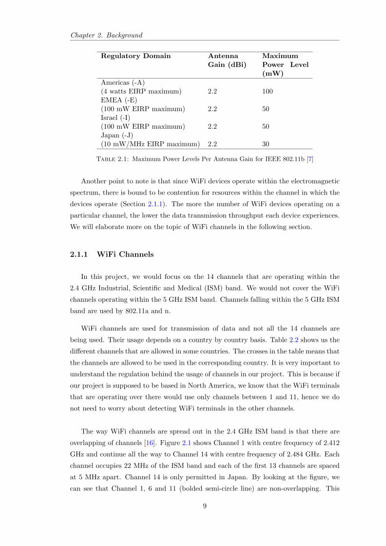
As part of the standards, there is a limit on the power output levels of radio frequency
devices. Table 2.1 shows us the maximum power level allowed by the different regulatory
domains. Such a limit is placed so that a wireless transmitter is not allowed to operate
using a higher transmission power in order to increase the range of transmission. Since
our project involves detecting the presence of WiFi terminals, too much interference in
the environment would prevent us from accurately track the terminals. Hence, there
is a need to consider the different types of environment the monitoring APs would be
deployed. For example, the transmission range in an open space would normally be
longer than that in an indoor environment, where there are many other wireless devices
operating, which causes interference.
1From here on, we would refer the network environment that conforms to IEEE 802.11 standards,which provides network access via APs deployment in the environment, as WLAN.
8
Chapter 2. Background
Regulatory Domain AntennaGain (dBi)
MaximumPower Level(mW)
Americas (-A)(4 watts EIRP maximum) 2.2 100EMEA (-E)(100 mW EIRP maximum) 2.2 50Israel (-I)(100 mW EIRP maximum) 2.2 50Japan (-J)(10 mW/MHz EIRP maximum) 2.2 30
Table 2.1: Maximum Power Levels Per Antenna Gain for IEEE 802.11b [7]
Another point to note is that since WiFi devices operate within the electromagnetic
spectrum, there is bound to be contention for resources within the channel in which the
devices operate (Section 2.1.1). The more the number of WiFi devices operating on a
particular channel, the lower the data transmission throughput each device experiences.
We will elaborate more on the topic of WiFi channels in the following section.
2.1.1 WiFi Channels
In this project, we would focus on the 14 channels that are operating within the
2.4 GHz Industrial, Scientific and Medical (ISM) band. We would not cover the WiFi
channels operating within the 5 GHz ISM band. Channels falling within the 5 GHz ISM
band are used by 802.11a and n.
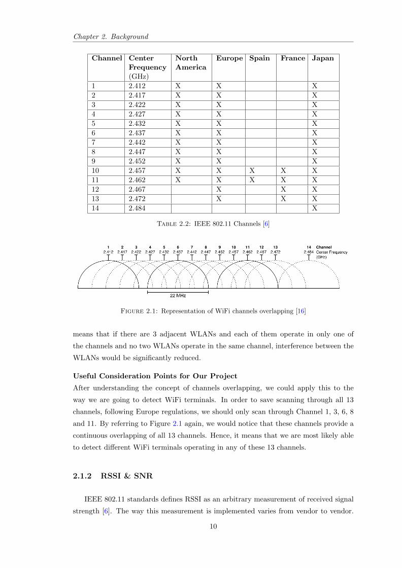
WiFi channels are used for transmission of data and not all the 14 channels are
being used. Their usage depends on a country by country basis. Table 2.2 shows us the
different channels that are allowed in some countries. The crosses in the table means that
the channels are allowed to be used in the corresponding country. It is very important to
understand the regulation behind the usage of channels in our project. This is because if
our project is supposed to be based in North America, we know that the WiFi terminals
that are operating over there would use only channels between 1 and 11, hence we do
not need to worry about detecting WiFi terminals in the other channels.
The way WiFi channels are spread out in the 2.4 GHz ISM band is that there are
overlapping of channels [16]. Figure 2.1 shows Channel 1 with centre frequency of 2.412
GHz and continue all the way to Channel 14 with centre frequency of 2.484 GHz. Each
channel occupies 22 MHz of the ISM band and each of the first 13 channels are spaced
at 5 MHz apart. Channel 14 is only permitted in Japan. By looking at the figure, we
can see that Channel 1, 6 and 11 (bolded semi-circle line) are non-overlapping. This
9
Chapter 2. Background
Channel CenterFrequency(GHz)
NorthAmerica
Europe Spain France Japan
1 2.412 X X X
2 2.417 X X X
3 2.422 X X X
4 2.427 X X X
5 2.432 X X X
6 2.437 X X X
7 2.442 X X X
8 2.447 X X X
9 2.452 X X X
10 2.457 X X X X X
11 2.462 X X X X X
12 2.467 X X X
13 2.472 X X X
14 2.484 X
Table 2.2: IEEE 802.11 Channels [6]
Figure 2.1: Representation of WiFi channels overlapping [16]
means that if there are 3 adjacent WLANs and each of them operate in only one of
the channels and no two WLANs operate in the same channel, interference between the
WLANs would be significantly reduced.
Useful Consideration Points for Our Project
After understanding the concept of channels overlapping, we could apply this to the
way we are going to detect WiFi terminals. In order to save scanning through all 13
channels, following Europe regulations, we should only scan through Channel 1, 3, 6, 8
and 11. By referring to Figure 2.1 again, we would notice that these channels provide a
continuous overlapping of all 13 channels. Hence, it means that we are most likely able
to detect different WiFi terminals operating in any of these 13 channels.
2.1.2 RSSI & SNR
IEEE 802.11 standards defines RSSI as an arbitrary measurement of received signal
strength [6]. The way this measurement is implemented varies from vendor to vendor.
10

Chapter 2. Background
This is because the standard does not make RSSI a compulsory element of it but leave it
as optional. This means that the rating that RSSI takes varies depending on which AP
vendor we are referring to. However, the vendor would have to provide the rating to the
device’s driver. The range that RSSI takes for Cisco devices, an AP manufacturer, is
between 0 and -120 [23]. The more negative the RSSI value is, the weaker is the signal.
The RSSI we are discussing here is measured in dBm.
SNR stands for signal-to-noise ratio. As you can probably understand simply from
this phrase, SNR gives the relative difference between the power level of the radio fre-
quency and the noise floor. Noise is the result of any devices or natural causes that
produce energy in the electromagnetic spectrum. 802.11 networks can cause interfer-
ence to each other, which is known as co-channel and adjacent channel interference [8].
However, networks that follows the IEEE 802.11 standards would generally work to-
gether harmoniously such as the sharing of the channel capacity if the networks are on
the same channel. The major cause of interference appears to be devices that operate
using the unlicensed band that does not belongs to 802.11 such as microwave oven and
Bluetooth devices.
SNR is an important parameter that we need to consider in WLAN. For example,
if the received signal strength is x in a low noise environment, x would decrease in an
environment with high noise, due to the interference affecting the transmitted signal. If
the noise level is close to the RSSI, this means that the signal would be corrupted.
Useful Consideration Points for Our Project
SNR is useful especially when we need to use RSSI to assist in localising a WiFi terminal.
An RSSI with a low value does not always mean that a terminal is far away from an
AP. We could make use of both RSSI and SNR to come up with a technique to localise
a device as accurately as possible.
2.1.3 Management Frames
There are 3 types of frames that is defined in IEEE 802.11, namely management
frame, control frame and data frame. In this project, we are more interested in the
management frames, which would shed some light on the possible ways we could de-
tect the presence of WiFi terminals. Management frames are used for the purpose of
establishing a connection between an AP and a terminal. A terminal in a WLAN, with
multiple APs deployed, may move around and as a result, the terminal may need to
switch association from one AP to the next using management frames. In addition, the
usage pattern and the type of Operating System(OS) of a terminal would also trigger
11
Chapter 2. Background
some of these management frames to be sent either occasionally or regularly. For in-
stance, a smartphone may be in sleep mode initially. When it wakes up, it would send
out a probe request frame to determine whether there are any APs nearby with sufficient
signal quality for it to associate. On the other hand, the OS of the smartphone may
choose to send out probe request frame every now and then to determine whether there
are any APs nearby that would provide better signal quality. Probe request and response
would be covered further in Section 2.1.4.
Apart from probe request frame, there is also the beacon frame, which is being
broadcasted by each of the APs in WLAN in a regular time interval. A beacon frame [17]
consists of frame header like any other frames, which includes the source and destination
MAC addresses. It also contain information such as beacon interval and Service Set
Identifier (SSID), which is the name of the WLAN. The SSID is important for a terminal
to know which network it is trying to establish a connection with. A beacon frame allows
a terminal to be aware of the APs nearby so that it could choose whether to associate to
it. The terminal is able to work out which AP has a better signal quality by determining
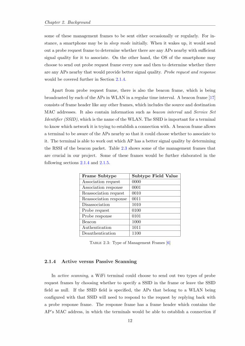
the RSSI of the beacon packet. Table 2.3 shows some of the management frames that
are crucial in our project. Some of these frames would be further elaborated in the
following sections 2.1.4 and 2.1.5.
Frame Subtype Subtype Field Value
Association request 0000
Association response 0001
Reassociation request 0010
Reassociation response 0011
Disassociation 1010
Probe request 0100
Probe response 0101
Beacon 1000
Authentication 1011
Deauthentication 1100
Table 2.3: Type of Management Frames [6]
2.1.4 Active versus Passive Scanning
In active scanning, a WiFi terminal could choose to send out two types of probe
request frames by choosing whether to specify a SSID in the frame or leave the SSID
field as null. If the SSID field is specified, the APs that belong to a WLAN being
configured with that SSID will need to respond to the request by replying back with
a probe response frame. The response frame has a frame header which contains the
AP’s MAC address, in which the terminals would be able to establish a connection if
12
Chapter 2. Background
it chooses to. If the SSID field of a probe request frame is left as null, any APs in
the surrounding that is configured to respond to such frame would reply with a probe
response. However, for security reasons, it is possible that APs would not respond to
such frame.
In passive scanning, the terminal would listen for any beacon frames that are being
broadcasted by nearby APs. The terminal might receive multiple beacon frames from
different APs. In this case, the terminal would make use of RSSI to determine which
AP it should associate to.
Useful Consideration Points for Our Project
As we might notice, since terminals are sending out probe request frames every now
and then, it is highly that we could make use of these probe request frames to detect
terminals. Furthermore, a probe request frame also contains the source MAC address in
the frame header, which means that we can identify a terminal easily since MAC address
is globally unique.
2.1.5 Joining and Leaving a WLAN
The Join Process [9] involves 3 stages before a terminal could start sending data over
WLAN. The first stage involves discovering an AP to begin establishing a connection.
The second stage requires the authentication of the terminal . There are two types
of authentication methods, namely open authentication and shared key authentication.
Open authentication does not involve any true authentication at all and the AP would
just reply to any authentication frames it receives. Shared key authentication, as the
name implies, makes use of a common key for the authentication process. The wired
equivalent privacy (WEP) key is used for authentication but is currently the most in-
secure way. However, in order to meet the IEEE 802.11 standards, WEP is still being
implemented by AP vendors. Other more secure authentication methods are available
such as EAP and WPA.
The third stage involves the association process before data transmission through
the network can take place. The main part of this process involves the terminal sending
an association request frame to the AP, in which the AP would reply back with an
association response frame if everything goes well.
There are also other processes such as reassociation, deassociation and deauthenti-
cation. Reassociation happens when a terminal moves beyond the range of an AP to
another AP that is still within the WLAN. Reassociation is similar to association but
the APs within the WLAN would transfer the information of the terminal between each
13

Chapter 2. Background
other. On the other hand, dissociation and deauthentication happens when a terminal
is disconnecting from a WLAN. A dissociation frame and deauthentication frame are
sent to the AP the terminal is previously connected to.
Useful Consideration Points for Our Project
The process of association and dissociation could form a good mechanism for detecting
the presence of a terminal within a specified WLAN. This is because the association of a
terminal to an AP is a good indication of the relative location of the terminal to the AP.
Using this association information with RSSI, we would be able to localise a terminal
easily. The dissociation process would mark the end of a terminal’s existent near an AP.
Furthermore, with the reassociation process, we could easily track the movement of WiFi
users from one AP to the next. However, there are a few shortfalls in this mechanism.
For instance, a terminal may not attempt to reassociate to a closer AP after moving
away from the previous AP it associated to due to the way its association algorithm is
implemented. This is further discussed in Section 3.2. We will also be evaluating the
different mechanisms that can be used in detecting the presence of WiFi terminals in
Chapter 4 on Design.
2.2 Wireless Chipset and Network Interface Card (NIC)
This section will discuss some of the major wireless chipset manufacturer for both
APs and other WiFi devices. In particular, we would focus on the chipset for APs since
we are going to implement a solution using off-the-shelf WiFi APs. We would like to
discuss about the chipset manufacturers so that we could decide on one that is widely
adopted by most of the AP manufacturers2.
2.2.1 Types of Chipsets
There are a few top semiconductor vendors that manufacture chipsets for APs. Al-
though there are many brands such as Cisco LinkSys, TP-Link, NETGEAR and D-Link,
which manufacture APs, the chipsets that these AP manufacturers use could come from
a few major semiconductor vendors. We have listed these vendors below:
• Broadcom - Based in USA and manufacture most of the 802.11 chipsets for
a variety of AP manufacturers. Most of Broadcom chipsets are used in Cisco
LinkSys, Buffalo and Belkin APs. Broadcom has a huge success with the high sale
of APs from Cisco LinkSys. It has a good device driver which is available for use.
2Note that chipset manufacturers are not the same as AP manufacturers. For example, Cisco LinkSysuses both Broadcom and Atheros in different models of its APs.
14

Chapter 2. Background
The broadcom-wl driver allows us to perform many operations that are offered by
the chipset. [4]
• Qualcomm Atheros - Also based in USA and its chipsets are used mainly by
TP-Link and D-Link. Atheros has two main drivers which allows us to invoke
some operations on the chipset. They are ath5k and ath9k. [27]
• Ralink - Bought over by a Taiwanese company MediaTek and famous for manu-
facturing WLAN chipsets. Its chipsets are used only in some model of D-Link and
TRENDNet.
A typical AP that we have used in this project has a specification as listed in Table
2.4. As we can see from the table, there are really a limited amount of space that we
can use for executing our code on the AP for this project. Although we do have other
newer models of APs that has slightly higher specification, we want to aim to keep our
program as small as possible, making use of the limited CPU performance, RAM and
flash storage space.
Feature Information
CPU 125MHz
Architecture MIPS32TM
RAM 16MB
Flash storage 4MB
WLAN NIC Broadcom BCM4306
WLAN standard b/g
Table 2.4: Specification of an AP
2.2.2 List of Broadcom Chipset Commands
Command Description
wl -i eth1 status Gives information about the network interface specified,eth1. This includes MAC address associated with this net-work interface
wl radio Get status of radio
wl radio on Turn on radio
wl ap 0 Set AP in client mode
wl ap 1 Set AP in Access Point mode
wl assoclist Retrieve MAC addresses of associated devices
wl rssi 〈 MAC addr 〉 Get RSSI for the terminal with the specified MAC address
wl channel n Set the channel to n
Table 2.5: List of Broadcom chipset Commands [10]
The Broadcom device driver provides functions that we can call from within the
custom OS. Some of these functions are essential for instructing the chipset to carry out
15
Chapter 2. Background
certain operations we require in order to detect the presence of terminals. Some of these
commands are illustrated in Table 2.5.
2.2.3 NIC modes
For a particular model of NIC, there are a few possible modes of operation. They are
AP Infrastructure, Client, Repeater, Ad-hoc or monitor mode. When we place the AP’s
NIC into monitor mode, the NIC would pass all packets it receives to the OS without
any filtering [24]. This means that we can pick up management frame such as probe
request frame, which we have mentioned earlier in Section 2.1.4 (Active versus Passive
Scanning) that we can use probe request frames as a mechanism to detect the presence
of terminals near an AP.
2.3 Custom OS for AP
In this section, we evaluate some of the open source OSs that allow us to make
customisation and install it to an AP. Custom OS is required because the originally
shipped OS from AP manufacturer usually do not provide SSH or telnet access to the
AP’s OS. Even if we can have access to the OS, it is extremely hard to write a program
to be executed on the AP shipped with the manufacturer’s OS. We will look at two
different freely available OSs that we could use to replace the originally shipped OS
below.
2.3.1 DD-WRT
DD-WRT is an open source Linux-based OS for wireless router and embedded sys-
tems [3]. This OS is very powerful and stable which was released back in 2005 and is still
in continuous development by the author and other open source developers. DD-WRT
has a few major releases which saw its code base being changed completely. The latest
version of the OS makes use of Open-WRT[14] kernels which in turn builds on top of
the original Linksys WRT54G V1 router OS which was released as open source software
under GNU General Public License. This means that the OS is very stable since it has a
solid foundation. This OS supports Broadcom, Qualcomm Atheros and Ralink chipset.
These chipsets are mainly based on MIPS architecture.
The main language that is supported natively on DD-WRT OS is C programming
language. C is a powerful language and the OS also supports dynamic memory allocation
feature of C. This is very useful because it allows developers to write memory efficient
16
Chapter 2. Background
code, i.e., allocate memory only when required. Although the chipset may only have
one processor, the OS supports concurrent execution of programs by interleaving the
execution of the processes. There is also feature such as forking, which creates a new
child process that is a duplicate of the original calling process. The main challenge to
writing a program to execute on DD-WRT OS remains to be the cross compiling stage.
Cross compiling involves using a toolchain on a build machine to compile an executable
binary program to be run on a different platform, which is different from the platform
of the build machine.
There are two types of storage space that can be used within the AP. One is the
Random-access memory (RAM) which operates just like the normal RAM on common
computers. Another is called the Flash memory which allows the storage of files per-
manently even when the AP is turned off. There is also Non-volatile random-access
memory (NVRAM) available which provides a good place to store configuration settings
or any other information for a program and this information can be accessed easily by
calling a command available in C. The information that has been saved on NVRAM will
stay on even after the AP is switched off and back on again.
Within the OS, there are two different types of file system. One is non-writable and
the other is re-writable. Journalling Flash File System (JFFS/JFFS2) is a re-writable
area on an AP’s OS. This filesystem is very useful for developers because it enables them
to use C Input/Output (IO) library like the following example:
fopen - Open an existing file or create a new one
fread - Read the content of the opened file into a buffer
fwrite - Write content from a buffer to a file
Not only the main IO operations can be carried out using the functions above, there
are many other useful things that can be accomplished on DD-WRT OS, thus enabling
us to develop a powerful program to be run on the AP.
2.3.2 OpenWrt
OpenWrt is another linux distribution for embedded devices. It supports Broadcom,
Qualcomm Atheros, Ralink and Intel chipset. OpenWrt provides a framework for de-
velopers to build applications around it [14]. OpenWrt is licensed as a free and open
source software under GNU GPL and is actively driven by the community.
OpenWrt provides a very easy tool to install new features to the AP by using a
package management tool. This tool makes installation of new program on the AP a
17
Chapter 2. Background
breeze just like how one would do on Ubuntu Linux Operating System, i.e., using apt-get
install PROGRAM-NAME.
Since the later version of DD-WRT builds on top of OpenWrt, most of the func-
tionality that OpenWrt has also appears on DD-WRT OS. However, DD-WRT has a
broader functionalities which OpenWrt seems to be lacking in some areas. Other than
that, OpenWrt supports program written in C and it also supports concurrent execution
of processes.
2.4 Related Wireless LAN Software tools
In this section, we would look into some of the available software tools and libraries
that are related to the capturing of data, management and control frames. Some of these
tools require a particular model of NIC in order to work. Later on, we would summarise
and evaluate which tools might be useful for us to explore and use if appropriate.
2.4.1 Kismet
Kismet is a free wireless network sniffer and detector program [34], which detects
wireless network even those that do not broadcast their SSIDs. It can determine the
range of IP addresses of a wireless network. Another good thing about Kismet is that
it could pick up 802.11 management frames for a wireless network. Kismet is mainly
used for locating APs within a WLAN, troubleshoot a WLAN and as a site survey tool
for learning about the received signal strength at different spots within a WLAN. This
allows network administrators to decide how to deploy APs within a defined area.
Apart from using it as a site survey tool, it could also be used to pick up probe request
frames which are sent out by WiFi terminals. Kismet sniff network packets passively.
It places the NIC into monitor mode so that it could pick up any management frames
that are broadcasted by either terminals or other APs. Kismet runs on Linux OS but
requires that the computer it runs on has a compatible NIC.
2.4.2 NetStumbler
NetStumbler is free but not available as open source. It is a tool for detecting and
finding APs around an area. It works slightly different from Kismet because it tries
to find APs actively by broadcasting a probe request frame with the SSID field filled
with the name “ANY” [35]. This creates a problem when the APs are configured not
18

Chapter 2. Background
to broadcast their SSID, hence they would not respond to a probe request frame with
SSID as “ANY”. For this reason, Kismet could detect more APs than NetStumbler.
2.4.3 Wireshark
Wireshark is a network packet analyser [38], which provides a very detailed GUI for
interpreting and analysing of network packets. The network packets could come from
any network interfaces of the computer which runs Wireshark. These includes both LAN
and WLAN. It also supports placing a NIC into monitor mode, which then allows the
capturing of management frames. Wireshark uses pcap, a software library for capturing
network packets.
Wireshark seems to be more suitable for network administrator to analyse network
traffic or find out problems that occur within the network. It provides a very nice GUI
with advanced sorting and filtering of each record representing a network packet.
2.4.4 Wiviz
Wiviz is a wireless network visualisation tool [32], which works pretty much like
Kismet. However, Wiviz is an old tool that has not been updated since 2005 and is no
longer working on many of the newer models of APs. Wiviz is able to place NIC into
monitor mode just like Kismet, in order to pick up probe request frames that are being
broadcasted by nearby terminals.
2.4.5 Tcpdump and libpcap
Tcpdump, as its name implies, is a powerful command-line tool for capturing and
dumping of network packets on a Linux machine. On the other hand, libpcap is a
C/C++ library for capturing network packets, which works by accessing the low-level
packet capture utility of the OS [22]. The library provides a high level interface for
accessing the packets that comes in through the NIC. There are many functions available
via this library which makes it one of the most powerful packet capture library ever.
Even Wireshark and Kismet also makes use of this library. When NIC is placed into
monitor mode, NIC would supply all the frames it receives, which also include the header
frame that contains MAC address information. pcap_can_set_rfmon() could be used
to check whether a NIC can be placed into monitor mode. If NIC cannot be placed into
monitor mode, the libpcap would only be able to capture normal network traffic but not
management frames such as probe request and beacon frames.
19

Chapter 2. Background
2.4.6 Summary
We could see that there are a variety of tools out there that are mostly open source
and relates to packet capturing. However, since these tools involve code base that spans
more than hundreds of source files, some tools would not be that easy to fork and
modified it to work according to the objectives that we have for this project. There is a
need to consider the feasibility of understanding and getting a piece of tool or library to
work. This usually only happens after we experiment with trying the tools. In Chapter
5 (Implementation), we would discuss about the experimentations that we have with
some of these tools, in which we have to try them on different models and brands of
APs. It would be slightly easier if we choose to implement our project using a PC or a
laptop, since we can see from above that most softwares are compiled to work on either
Linux or Windows OS of a computer.
2.5 Data Transmission
Since this project involves deploying APs in multiple locations so that they could
detect the presence of WiFi terminals, we need a way to transmit all the collected data
from each AP to a central server for processing. Since our project involves creating a
program to run on an AP, which is an embedded device running on a different computer
architecture with limited computing resources, we need a good serialisation method and
a data transmission library that has little memory footprint and utilises low flash storage
space.
2.5.1 Serialisation of Data
Before client and server could exchange messages using TCP or UDP, the data has to
be serialised into a stream of bytes so that they could be stored or sent later [25]. After
transmitting the messages over to the other party, these messages have to be deserialised
into appropriate data structures that is understandable. Over the years, there have been
many methods for serialising data and a few prove to be the most adopted either for
their convenient uses, example JSON, or for their great efficiency in terms of storage and
parsing speed, example Protocol Buffers. Below gives detail about some of the possible
serialisation methods that we could use in this project.
1. Tab-delimited: If the structure of the data that we are going to transmit is not
that complex, it is possible to simply use tab-delimited technique, which stores
values in rows and columns and for each row, the values are separated by a tab
20
Chapter 2. Background
space. Each row is considered a string and there is a newline character at the end
of the string to mark the end of the row. This format is simple but since it is
too simple, it is not good enough to represent complex data structures. It is also
not efficient for reading and writing data, which mostly involve carrying out string
operations such as concatenation and splitting.
2. JSON: It is a lightweight data exchange format that makes use of key-value pairs
extensively. JSON is supported by many programming languages, which provide
native serialising and deserialising of the data stored in JSON format. It is a
human-readable form that is easy to understand by simply looking at the data
stored in this format alone. This is also partly the reason why most web appli-
cations tend to use JSON for client-server data exchange. Most of the big web
applications such as Flickr, Tumblr, Instagram and Facebook provides a REST
API that returns data in JSON format.
3. Protocol Buffers (PBs): It is a method of encoding structured data in an
efficient, yet extensible format [5]. PBs are developed by Google and are used
extensively in Google for almost all its applications. The way PBs work is by
defining an Interface Definition Language (IDL) file stored in .proto format, which
serves to describe the structure of the data that is being stored. PBs are designed
to be fast, efficient and simple. The data that is serialised using PBs is much
smaller than XML3. Google reports that PBs are 3 to 10 times smaller than XML
and the time to parse data in PBs is 20 to 100 times faster than that for XML.
Storage space and parsing time are two crucial elements that we want to consider
when deciding which serialisation format to use for serialising data on each AP so
that it could be sent to a central server.
4. Nanopb: It works the same as PBs but Nanopb is a C-based implementation of
PBs with small code base [26]. It is built with the constraints of embedded devices
in mind with low memory and small flash storage space. In particular, Nanopb
targets 32-bit microcontroller. Nanopb encodes and decodes data in almost the
same way as PBs, using a slightly similar proto IDL file as its template for encoding
and decoding data. It is possible to encode data using Nanopb on embedded device
and decode the data on another machine using Google BPs with slight changes to
the proto file.
2.5.2 File Transfer Library for Embedded Devices
cURL stands for Client for URLs. It is a project started in 1997, which develops
the libcurl library, a client-side URL transfer library [11]. It supports many application
3XML is a format for data serialisation. It is too verbose and takes up a lot of space.
21

Chapter 2. Background
protocols such as FTP, FTPS, HTTP, HTTPS, IMAP, IMAPS, POP3, RTMP, RTSP,
SCP, SFTP, SMTP, TELNET and TFTP. Furthermore, it supports important HTTP
methods such as the GET, POST and PUT. This makes it a very powerful client-side
library and also an ideal library for data transmission over the internet using HTTP or
HTTPS protocols. Another good thing about libcurl is that most of the file transfer
errors or exceptions are properly managed and handled in a graceful way.
2.6 Storing and Aggregating Big Data
As we need to store the collected data from each AP for later processing and querying
from a GUI for displaying the statistical view of the aggregated data, we need to select
a suitable database that fits our use case, i.e., ever growing amount of data collected.
We also need to understand the available data analytic methods that would allow us to
aggregate our data efficiently.
2.6.1 Relational SQL versus NoSQL database
10 years ago, the terms Big data and NoSQL are probably not as often heard as
today. These words are appearing everywhere on the internet because of the exponential
growth in the amount of data that is being generated within the last few years alone.
More and more data is accumulated due to more user interactions on the web, example
via Twitter or Facebook, increasing amount of server logs, generation of more scientific
data such as gene sequencing and analysis, as well as more Wireless Sensor Networks
(WSNs) being deployed. This means that there is a need for a new way to handle this
data, which leads to the adoption of the widely used Hadoop Distributed File System,
which is a distributed file system modelled after the Google File System and has the
capability to scale across thousands of machines.
NoSQL is based on the idea that it can scale massively, provide very fast write
operations, quick key-value pair lookups and has very flexible data types and schema.
Most of the NoSQL implementations do not require the developer to specify the types of
the data to be stored in advance and this is one of the beautiful characteristics of NoSQL.
In addition, it does not provide any ACID-compliance transaction feature, which helps
to boost its read and write performance tremendously. Since tracking user mobility
involves collecting data from each AP, which could increase to hundreds of them in
commercial roll-out, a NoSQL database is an ideal choice. Furthermore, since we are
not dealing with data that involves transaction such as bank account details, we do not
need the strict consistency of relational SQL.
22
Chapter 2. Background
Relational SQL has a strict schema that we need to follow. The data types for each
attributes have to be defined in advance when creating the table. It provides feature such
as join operation and transactions, which observe the ACID properties4. Furthermore,
it provides easy-to-use SQL query language, which allows developers to query data from
the database simply by writing a SQL statement. MySQL is a relational database
management system (RDBMS), which is free and open sourced. MySQL is powerful up
to a certain point when the amount of data becomes too much for it to handle. In order
to scale its capacity up, it would involve the deployment of a master node, which handle
write operations, and slave nodes that take care of read operations. Data from master
node will be replicated to the slave nodes.
2.6.2 NoSQL Databases
In this section, we would discuss in further detail the different types of NoSQL
solutions available so that we can make a more informed choice of choosing one, which
is the most suitable for the nature of our project and not just for our initial prototype.
It should be noted that the explanation of how HBase works below would aid in the
understanding of Chapter 5 (Implementation), in which we use HBase for our data
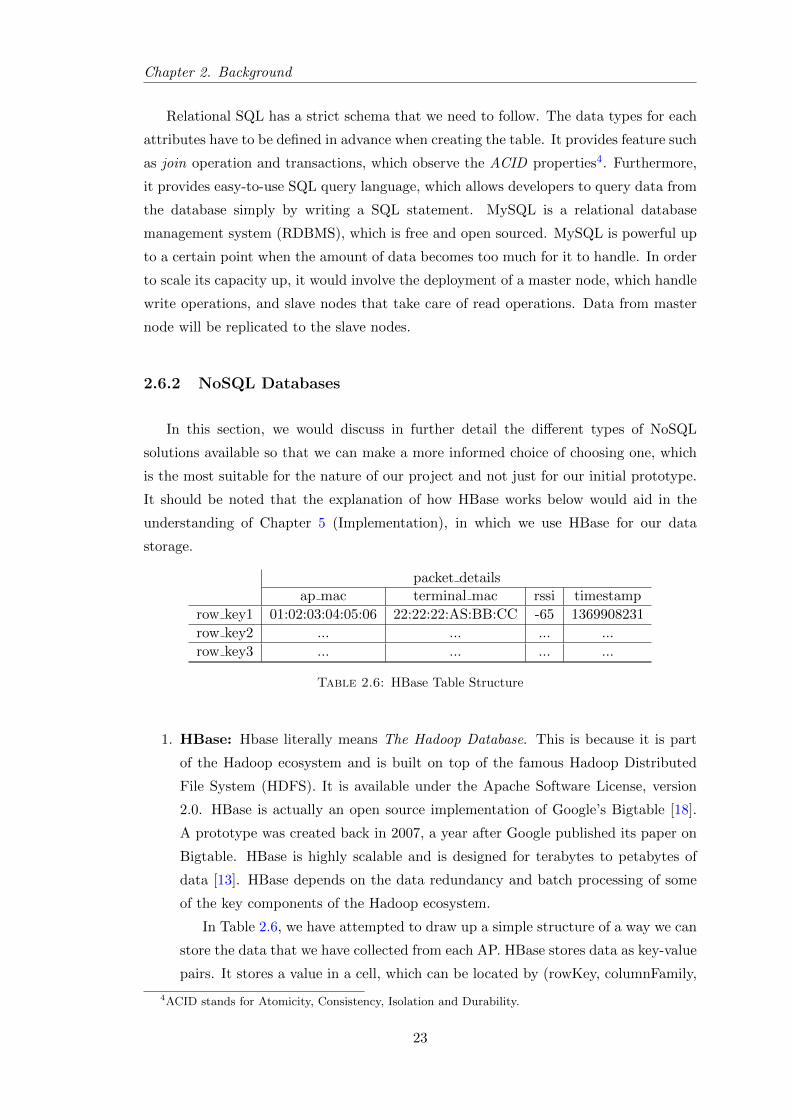
storage.
packet detailsap mac terminal mac rssi timestamp
row key1 01:02:03:04:05:06 22:22:22:AS:BB:CC -65 1369908231
row key2 ... ... ... ...
row key3 ... ... ... ...
Table 2.6: HBase Table Structure
1. HBase: Hbase literally means The Hadoop Database. This is because it is part
of the Hadoop ecosystem and is built on top of the famous Hadoop Distributed
File System (HDFS). It is available under the Apache Software License, version
2.0. HBase is actually an open source implementation of Google’s Bigtable [18].
A prototype was created back in 2007, a year after Google published its paper on
Bigtable. HBase is highly scalable and is designed for terabytes to petabytes of
data [13]. HBase depends on the data redundancy and batch processing of some
of the key components of the Hadoop ecosystem.
In Table 2.6, we have attempted to draw up a simple structure of a way we can
store the data that we have collected from each AP. HBase stores data as key-value
pairs. It stores a value in a cell, which can be located by (rowKey, columnFamily,
4ACID stands for Atomicity, Consistency, Isolation and Durability.
23
Chapter 2. Background
columnQualifier) coordinates of the table. This is analogous to a 3-dimensional
array. These 3 terms are crucial terms that we would used extensively in Chapter 5
(Implementation) to explain how we retrieve values from the table for aggregation.
In Table 2.6, row key1 is a row key, packet details is a column family and ap mac,
terminal mac, rssi and timestamp are column qualifiers. Under a column family,
we could have as many column qualifiers as possible and when we mention many,
it refers to millions of them. As for the number of rows, we can have billions of
them in a table. This is why we have said earlier that HBase is highly scalable.
We could define as many column family as we need but this parameter should be
kept to a minimum. As an example, we can have another column family such as
extra information, which would hold column qualifiers such as ap GPS coordinates
and ap nearest building.
HBase is very flexible on the data types and schema of the table. Each cell
of the table could be data in any formats since HBase store them as bytes. This
means that we can store the content in a cell as Integer and later replace the
data type of the cell to String without any problems. HBase does not require
the developer to specify the column qualifier in advance, which is in contrast to
relational database that requires the specification of table attributes during table
creation. However, HBase does require the developer to specify the column family
in advance for a few reasons. One of them is that the content of a whole row might
not be stored on a single server. Each of the column families of a row would be
stored on a different RegionServer5.
Finally, since HBase uses HDFS as a filesystem for storing its data, it inherits
some of the features that are available in the Hadoop ecosystem. One of this is
the Hadoop MapReduce. HBase allows us to use the data stored in it as input to
the Map function and the output of the Reduce function could be inserted back
directly into HBase. We will elaborate more on MapReduce in the next section.
2. CouchDB: CouchDB is a new type of database management system that stores
data as “documents”, in which we can call this as “self contained” data [1].
CouchDB is very relaxed on the schema of the data model. Let’s us use the
example of receipts to explain the concept behind CouchDB. Let say we have 5
receipts from different shops and they are all of different formats, i.e., some may
contain the fax number of the shop, some may not and some may contain other
details. All these receipts would be analogous to the documents in CouchDB. Each
document may contain different informations and does not have to follow the same
structure. We can have a fax number field in one document and not having it in
another. We can add more data to a document at a later time or remove some
5RegionServers are just servers that host small chunks of the HBase tables for the purpose of highavailability and scalability.
24
Chapter 2. Background
data without affecting other documents since the structure of each document can
be different. This is one of the beautiful elements of CouchDB, which makes it a
very flexible data storage system.
If we use the example in Table 2.6, each row would be stored as a separate
document. We may add extra details such as GPS coordinates of an AP to a
document and not have this detail at all in another.
However, the downside of CouchDB is that it uses too much space to store each
document. In Chapter 5 (Implementation), we have attempted to experiment with
the use of CouchDB and HBase and we compare the size of disk space used for
storing the data we collected from APs for each type of database. Apart from
using a lot of space, the only way we can communicate with CouchDB is by
making HTTP/HTTPS request via its extensive REST API. Adding, retrieving
and deleting data on CouchDB has to be done by this way, which is also its shortfall
since HTTP/HTTPS protocol is not a quick way for transmitting data across the
internet.
Lastly, CouchDB has a built-in MapReduce feature, in which the Map and
Reduce functions could be written in Javascript. CouchDB would apply the Map
function to each documents and the outputs from the Map function is passed on
to the Reduce function. We will discuss more about how MapReduce works in the
following section.
2.6.3 MapReduce Framework
MapReduce is a framework that uses functional programming concepts to process
large datasets in a parallel and distributed manner [36]. MapReduce was designed with
the aim of processing massive amount of data in a scalable manner. This means that as
long as we can afford to add more machines to process the data, its performance should
increase linearly [18]. MapReduce uses the divide and conquer approach to process
smaller chunks of data in parallel and at the end, these chunks would be aggregated to
produce a consolidated results.
Processing data using MapReduce involves two phases: the map phase and the
reduce phase. The input and output of both phases take the form of a key-value pair.
For MapReduce to work, we need to specify both the map function and the reduce
function.
• Map phase: The map function is executed once for each input key-value pair.
Within the map function, we could do some computation on the key-value pair
and at the end, we need to choose a new key to emit out. After the map function
25

Chapter 2. Background
is executed, MapReduce would sorts the output of the map function and group
together key-value pairs that have the same key and pass these to the reduce phase.
• Reduce phase: The reduce function is run once for each group of key-value
pairs that share the same key. This means that we have a bunch of data that
share certain similarities since we choose to emit them with the same key from
the map function. Hence, we could do some aggregation on the group of key-value
pairs such as adding up all the values together to find out the total sum. We can
then output the result with another key that we choose or we may also choose to
output the key that is passed into the reduce function.
Figure 2.2: Illustration of how MapReduce worksImages licensed under Creative Commons and GPL from iconfinder.com
In order to illustrate how MapReduce works, we have come up with an original
unique example to explain the concept as illustrated in Figure 2.2. Imagine that we
have a whole bag of gem stones, which could be hundreds of them, that are mixed
together. Each gem stone has a price tag attached to it. In this case, we consider the
colour of gem stone as the key and the price tag as the value.
Each of the gem stone is passed into the map function one by one, which could
happens in parallel. In the map function, the input key is gem stone colour and the
input value is the price. Within this function, we have a logic to accept only gem stone
that is worth more than £10. For gem stone worth more than £10, we will emit out
an output key which is the gem stone colour and an output value which remains to be
the price. For those worth lower, we will not emit out a key-value pair, i.e., we would
not pass the gem stone to the next phase and just throw it away. Note that we could
choose any parameter to emit out as key. If we have other information that is available
26
Chapter 2. Background
to the map function such as the continent the gem stone is found, we can even emit this
as output key.
Sorting will takes place after the map phase and all gem stone that has the same
colour will be grouped together since they share the same key.
In the reduce phase, each group of gem stones is passed into the reduce function.
The input key is the gem stone colour and input value is a bag of all gem stones of the
same colour with their price tags. Within this function, we have a logic to sum up the
total cost of all gem stones of the same colour. After finishing our aggregation, we will
output the key as gem stone colour and output value as the total cost that we have
calculated.
2.7 Summary
In this section, we begin by looking into what IEEE 802.11 standards are and we
go through the key components of the standards, which allow us to understand how we
can benefit from the standards. For instance, we could make use of the probe request
frames that are sent out by WiFi terminals to detect the presence of the terminals. Since
this frame also consists of MAC address of the terminals and it is possible for AP to
determine the received signal strength, using this mechanism to detect terminals is a
feasible approach. The association, reassociation and dissociation process could also be
an alternative way for us to detect the terminals although it has its shortfalls. We will
look into these shortfalls in Section 3.2 under Related Work, which we get to learn from
what other researchers have achieved via this mechanism and also its advantages and
disadvantages.
We also discuss some of the OSs available for embedded devices such as APs and
attempt to explain some of the functions provided by the chipset manufacturers via their
device drivers. After that, we looked at the different serialisation methods and the types
of databases system available as well as a framework for aggregating large datasets.
MapReduce is a good framework, which abstracts the complicated underlying schedul-
ing and parallelising of MapReduce tasks from the developers, allowing developers to
focus just on writing the logic for the map and reduce functions. Since HBase is built
on top of HDFS, there are many benefits that it gets apart from the scalability and
availability of the filesystem. This includes using HBase table as both source and sink
of a MapReduce job, i.e., the input can come from the table and the output gets writ-
ten to the table directly. Finally, since HBase is used by big web companies such as
27

Chapter 2. Background
Facebook for its messaging and StumbleUpon for its realtime analytics, it has an active
development environment, in which it will become very popular in the future.
28
Chapter 3
Related Work
Over the years, there have been numerous papers published about localisation using
various mechanisms. Attempts have also been make to track the movement of users car-
rying WiFi terminals within a pre-defined compound under the area of experimentation.
In this chapter, we explore the various mechanisms that other researchers have come
up with in order to track WiFi users movement. It would be helpful to go through and
evaluate others’ work in this field so that we could understand the terminologies, con-
straints and limitations of various mechanisms. Hence, from there, we could decide on a
better mechanism that is envisioned to address some of the constraints and limitations.
3.1 Mechanisms for Tracking WiFi Terminals
Real traces of users’ location can be used to derive a mobility model that would be
useful for researchers working on applications, systems or devices in which the movement
of users is significant to their work, especially for location-aware applications and network
optimisation. This provides the motivation for some researchers to look into tapping the
potential of using WiFi to track user mobility and from this data, they could generate
a user mobility model, which would be available to other researchers interested in the
data model.
Amongst the papers we have reviewed, we notice that there two main different mech-
anisms that are being used to track terminals’ location and network activity, in which
network packets are being monitored. We explain the two main ideas below.
1. One is the use of syslog at APs to record information regarding association and
dissociation of WiFi devices. syslog traces do not provide information regarding
the signal strength between client and AP. In order to obtain extra information re-
garding the network activity that a user engaged in, SNMP and tcpdump are being
employed to get the MAC address of devices and other information by capturing
the header of network packets [21]. This allows analysis of which application layer
protocols are being used by the users such as Hypertext Transfer Protocol (HTTP),
File Transfer Protocol (FTP) and Gnutella (Peer-to-peer).
29

Chapter 3. Related Work
How it works:
The APs are configured to send Syslog message whenever a user authenticate,
associate, dissociate and deauthenticate. User Datagram Protocol (UDP) is chosen
as the transport layer protocol. This means that error checking and correction
would not be carried out at the transport layer, thus, lowering the overhead. Apart
from syslog, Simple Network Management Protocol (SNMP) is used to poll the APs
every 5 minutes. MAC addresses, together with inbound and outbound traffic of
the recently associated clients would be returned in each poll. In addition, tcpdump,
is also used to sniff the wireless network traffic of the users. This tool captures the
packet headers, enabling more in-depth analysis of the network traffic to be carried
out. A sniffer server is placed in each major location for this sniffing purpose.
2. Another approach is a client-side implementation in which most of the logic is
being put on the user’s device. For instance, a smartphone would detect user’s
motion using accelerometer, environment light using device’s camera and sound
using microphone. The phone also collects information such as the presence of APs
nearby as fingerprint and all the information can be sent from the user’s device
across to a server for processing [2].
Fingerprinting works when the smartphone scans the surrounding for WiFi
APs. A fingerprint is formed from the list of MAC addresses that is being captured
by the phone in a short period of time. Based on a formula, this test fingerprint
will be compared with the one stored in the database as candidate fingerprint.
With the extra information provided by the smartphone, the logical location of
a phone user can be determined very accurately as opposed to just relying on GSM
or WiFi for localisation. This is because different environment looks differently
with a variety of different decorations and lightings. For instance, a pub can be
distinguished easily from a book store from the difference in light ambience. If only
GSM or WiFi is used to determine the user’s location, it could lead to ambiguity.
For example, if there are two shops, A and B, next to each other, a user entering
Shop A may mistakenly be interpreted as entering Shop B and vice versa. This
ambiguity cannot be ignored if the shop owner wants to use the localisation data to
send the user coupons or there is a need to aggregate the number of users visiting
each shops.
A user may also move differently in different types of shops. For example, a
person visiting the supermarket may move up and down the rows frequently while
a person visiting a restaurant may move only for a short distance before sitting
down. The accelerometer helps to detect the user’s movement.
30
Chapter 3. Related Work
3.2 Factors Affecting Accuracy of Detecting WiFi Termi-
nals
Since we need to estimate the location of a user, we may also need to consider some
of the factors that would affect the accuracy of our estimation. The first two factors
discussed below is more relevant for using association and dissociation of a terminal from
an AP as a detection mechanism. The last three are general phenomenons that would
not be easy to solve.
1. A user’s terminal may be associated to an AP but it may not be close to the AP.
Furthermore, the terminal might not associate to an AP that is closest to it in
terms of real distances [19]. This is due to the fact that different terminals have
different algorithm regarding AP association, i.e., it might not choose to associate
with the closest AP.
2. Different terminals may have different level of reluctance to change association.
For example, Cisco VoIP phone tends to stay connected with an AP for a longer
time than other mobile devices. This highlights a factor which could potentially
affects the accuracy of tracking users since different users uses different models of
mobile devices.
3. The AP may be blocked by an object, thus the received signal strength by AP
from a terminal may be lower than it should be. This means that using just RSSI
in estimating a terminal’s location would not be accurate anymore.
4. Different environments have different levels of interference. The noise in one en-
vironment may be higher than in another due to the existent of many wireless
devices transmitting electromagnetic waves.
5. There could be refraction, reflection, diffraction, absorption and scattering of radio
signal, which causes the signal strength to be weaken [6].
Thus, all these factors may affect the location of a terminal being estimated, giving
us a false sense of the terminal’s location. For some of the problems above, they could
be resolved by using a different terminal detection mechanism such as the detection of
terminals by capturing the probe request frames that are being broadcasted rather than
using a terminal’s association and dissociation information.
31

Chapter 3. Related Work
3.3 Localisation Techniques
After reviewing some of the related work, a common concern that has been brought
up is the accuracy of determining a user’s position using 802.11 radio signal. Thus,
a number of different mechanisms and algorithms have been devised to estimate the
position of the user. Some of the methods and algorithms are summarised briefly below.
• Triangle Centroid - Using three APs as points of reference to determine a user’s
position. This involves using 3 points of association with APs to accurately deter-
mine the user’s position.
• Ambience Fingerprinting - Making use of different sensors available on smart-
phones to provide additional information necessary to determine a user’s position
accurately. This works because different environments look and feel differently.
This includes the sound and behaviour of the user in the environment.
• Signal strength - Using signal strength value between a WiFi terminal and an AP
could allow us to estimate a user’s position to a limited extent. This assumes that
no obstructions occur between them.
3.4 Summary
The use of authentication, association, dissociation and deauthentication information
as a mechanism for detecting WiFi terminals is a good method but it lacks robustness.
This is because only those users who are able to authenticate and associate with the APs
could be tracked. If a user choose not to associate or unable to associate with one of the
AP, inaccuracies would be introduced in the tracking results because the results does
not reflect the real environment. This could be a problem for this project because we
aim to collect information about WiFi users in an 802.11 network environment without
requiring users to do anything on their devices. Furthermore, we want to track as many
users as possible within this environment so that we can derive useful statistics about
the users.
For client-side implementation, the approach is not scalable. This is because it is
very hard to persuade or even reach out to users to install an application. However, it is
useful to learn how a client-based solution could be developed in contrast to relying on
data collected from APs. For our project, a client-side solution may not be that useful
since our objective is to track users anonymously without asking them to do anything,
which would be ideal and is the solution we are looking for.
32
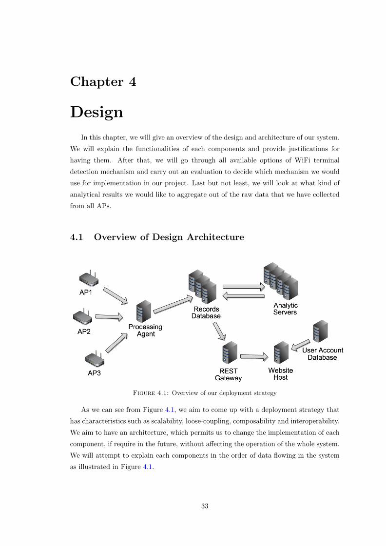
Chapter 4
Design
In this chapter, we will give an overview of the design and architecture of our system.
We will explain the functionalities of each components and provide justifications for
having them. After that, we will go through all available options of WiFi terminal
detection mechanism and carry out an evaluation to decide which mechanism we would
use for implementation in our project. Last but not least, we will look at what kind of
analytical results we would like to aggregate out of the raw data that we have collected
from all APs.
4.1 Overview of Design Architecture
Figure 4.1: Overview of our deployment strategy
As we can see from Figure 4.1, we aim to come up with a deployment strategy that
has characteristics such as scalability, loose-coupling, composability and interoperability.
We aim to have an architecture, which permits us to change the implementation of each
component, if require in the future, without affecting the operation of the whole system.
We will attempt to explain each components in the order of data flowing in the system
as illustrated in Figure 4.1.
33
Chapter 4. Design
1. AP: We will write a program to detect WiFi terminals that are close to each AP
that we have deployed. The job of the AP is to simply scan through each WiFi
channel, listen for incoming probe request frames that are being broadcasted by
terminals and send this information to the Processing Agent. The whole duration
of scanning and listening will take 30 seconds and all the information collected
is sent together once every 30 seconds. We will explain why we choose detecting
probe request frames as our detection mechanism later in Section 4.2.
We choose to send all the records1 together every 30 seconds to save the over-
head of establishing too many connections to the Processing Agent. We choose
to scan for 30 seconds to allow sufficient time for iterating through each WiFi
channels. This is because after some experimentations, any duration lower than
30 seconds would cause the AP to miss detecting some terminals.
A custom OS would be installed on each AP to run our program. This is
because the originally shipped OS with the AP does not allow us to run our
program on the AP. Finally, a file transmission library would be used to transmit
all the records to the Processing Agent. Such a library is needed because we want
to have the transmission error handling and exceptions of the library.
2. Processing Agent: At the Processing Agent, we have a REST API, which can
be invoked from each AP to upload the data collected. After we have received the
data from an AP, we will check the secret key that we have packed together with
the records. The purpose of using a secret key is to prevent a rogue AP that does
not belong to our system from uploading data to our Processing Agent, which
could results in a disastrous effect on our aggregated statistics. We will explain
how we implement the secret key more in detail in Section 5.2.3.
We decide to insert the timestamp for the records at the Processing Agent
before we push them to the database. This is because synchronisation of time on
the AP is currently not that reliable using a custom OS. If the clock time on the AP
is wrong, we will end up aggregating incorrect data, leading to false analysis of the
behaviour of users that we are tracking Hence, we decide to follow a more reliable
approach of inserting the timestamp at the Processing Agent. We understand that
there are disadvantages of this solution. Firstly, the granularity of detecting each
terminal would be about 30 seconds since the data collected by the AP is sent to
the Processing Agent every 30s and timestamp will only be inserted at that time.
Secondly, there is a possibility of some transmission delay, which would add to the
final timestamp for each record.
1From here on, when we mention records, we mean the unique WiFi terminal MAC address and itsassociated RSSI. Within the 30 seconds window, the AP may pick up multiple probe request frames fromthe terminal but we only consider the first one that we have captured. The terminal’s MAC address andRSSI forms a record.
34
Chapter 4. Design
Finally, we will push all these data to the database using the default protocol
for connecting to the database that we choose. Our choice of database would be
justified in the next chapter on Implementation. Note the arrow in Figure 4.1,
which shows that data only flow in one direction from the Processing Agent to the
database.
3. Records Database: This is the database that we will hold all the raw records
that we have collected from each AP and also the aggregated data that we are
going to generate by employing an analytic framework. The Records Database
should have the ability to scale easily because of the continuous stream of data
from all APs if we deploy them 24 hours a day and 365 days a year.
4. Analytic Servers: The Analytic Servers only has one main job to do, i.e.,
to aggregate the raw records that we have collected by fetching them from the
database and put the aggregated results back into the database. This explains
the two-ways arrows in Figure 4.1, which shows that data flows in both way. It
should be noted that we may also aggregate the data once, put them back into
the database and aggregate on the aggregated data again to derive a different
analytical model of the data. This is done this way because data from the first
aggregation may be used several times for generating different statistics.
5. REST Gateway: This component is subjective to the type of Records Database
and the front-end GUI that we are using. For our implementation in this project,
we require a REST2 Gateway. The database that we choose provides a client
library for retrieving data from code written in Java but not from any other lan-
guages. Although it also provides basic REST API for retrieving data via HTTP,
the REST API only allow simple querying of data and does not allow us to specify
the criteria such as what range of data we want to retrieve. Hence, we decide
to implement our own REST Gateway, which is written in Java so that we can
use the database Java client library to provide additional ways of querying data
from a GUI written in Javascript and HTML. For example, we allow the Web GUI
to specify the range of records, from which date to which date, that it wants to
retrieve. We aim to keep this description at minimal here in Design and will at-
tempt to explain them in detail later on in Section 5.6.1 under the Implementation
chapter.
6. Website Host: This will provide the hosting for our Web GUI, which has a back-
end written in PHP and front-end in Javascript and HTML. We need the back-end
to be in PHP because we want to provide login functionality for administrators
and business owners to login and check out the different statistics and graphs that
2REST is a software architecture that involves client-server, in which the server provides a standard-ised application programming interface for accessing and modifying data.
35

Chapter 4. Design
we have for them. Javascript is used in the front-end for querying data directly
from the database as we have mentioned earlier. Some element of HTML5 is also
used in this project. Javascript enables a website to look and operate just like an
app on the phone without having to refresh page often for selecting certain options
on the page. That is what we aim to achieve in our Web GUI.
7. User Account Database: This is implemented using a relational database for
account keeping purposes. We store the accounts for administrators and business
owners in this database as well as the APs that each account is allowed to view
the statistics associated with them.
4.2 Detection Mechanisms
In this section, we will outline the different mechanisms for detecting the presence of
WiFi terminals using what we have learnt from background and related work. We will
evaluate each mechanisms, highlighting any advantages or disadvantages, and justify
our choice of the mechanism we use for our implementation.
• Mechanism 1
Based on the association and dissociation records of a user’s WiFi terminal,
the MAC address of the terminal, and the time the terminal is detected can be
determined. If the AP does not use an open system authentication, the terminal
would have to authenticate itself first before association with the AP can take
place.
By using this mechanism, everything can be done entirely without the user’s
knowledge and that also means that this approach is practical. However, the
downside is that, only users who can associate with the AP will be tracked by this
mechanism. In addition, a terminal could still be associated to an AP even after
it has moved quite far away and not reassociate to a closer AP. This could be due
to its AP reassociation algorithm. This means that the data collected for deriving
the collective mobility of users will not reflects the actual environment.
• Mechanism 2
A terminal may send out probe request frames to search for nearby APs to
associate. The frame includes the MAC address of the terminal involved and we
can determine the received signal strength of the probe request frame on the AP.
With this information, we can localise a terminal to a certain extent of accuracy.
To explain Mechanism 2 visually and in an interesting way, we have come up
with an analogy for this mechanism, which we have chosen for our implementation.
36
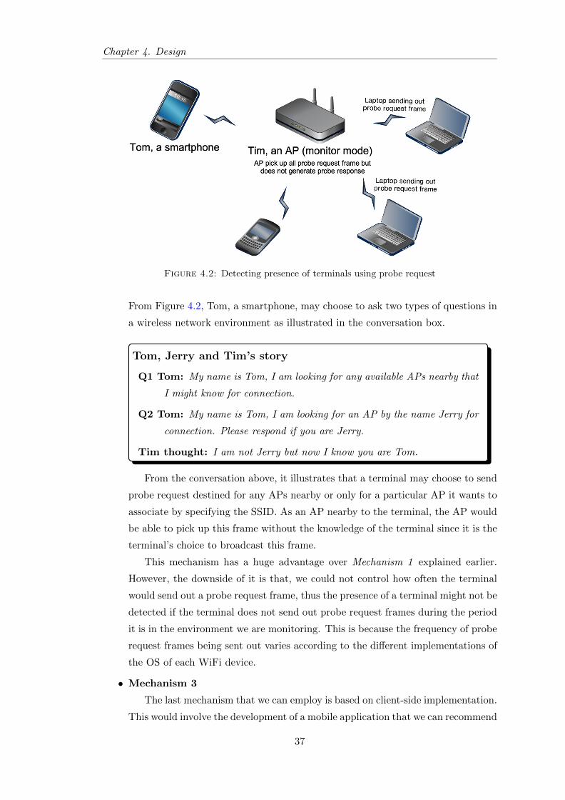
Chapter 4. Design
Figure 4.2: Detecting presence of terminals using probe request
From Figure 4.2, Tom, a smartphone, may choose to ask two types of questions in
a wireless network environment as illustrated in the conversation box.
Tom, Jerry and Tim’s story
Q1 Tom: My name is Tom, I am looking for any available APs nearby that
I might know for connection.
Q2 Tom: My name is Tom, I am looking for an AP by the name Jerry for
connection. Please respond if you are Jerry.
Tim thought: I am not Jerry but now I know you are Tom.
From the conversation above, it illustrates that a terminal may choose to send
probe request destined for any APs nearby or only for a particular AP it wants to
associate by specifying the SSID. As an AP nearby to the terminal, the AP would
be able to pick up this frame without the knowledge of the terminal since it is the
terminal’s choice to broadcast this frame.
This mechanism has a huge advantage over Mechanism 1 explained earlier.
However, the downside of it is that, we could not control how often the terminal
would send out a probe request frame, thus the presence of a terminal might not be
detected if the terminal does not send out probe request frames during the period
it is in the environment we are monitoring. This is because the frequency of probe
request frames being sent out varies according to the different implementations of
the OS of each WiFi device.
• Mechanism 3
The last mechanism that we can employ is based on client-side implementation.
This would involve the development of a mobile application that we can recommend
37
Chapter 4. Design
users to install. The application will download a list of MAC addresses of APs that
belong to us and if the mobile phone finds any one of these MAC addresses3, it
will send this information to our server. Hence, we are able to deduce the location
of the phone simply by associating its location to the the location of the AP or
APs.
This solution is the easiest to implement. However, it has many downsides.
Firstly, we would have to develop a range of applications for different mobile
platforms such as iOS, Android, Windows Phone and BlackBerry 10 in order to
track the users of these devices. Furthermore, there are many versions of computer
platforms to account for as well. Secondly, it would be extremely hard to persuade
a user to install the application so that we can track their whereabouts. They
would be highly unwilling to commit that, thus, this last solution is not very
practical.
This project aims to employ the best mechanisms to track collective mobility of users
in IEEE 802.11 environments, hence, Mechanism 2 explained above is being investigated
and implemented. This is because that mechanism does not require user interaction in
order for tracking to work. Furthermore, since most WiFi terminals would send out
probe request frames as part of their procedure to find nearby APs for association, we
would make use of this frame information to our advantage. This means that we would
be able to detect more terminals, which would give us a better representation of the
number of WiFi users in the environment under monitored.
The only downside to this mechanism is that since some terminals do not send out
probe request frames that often, it would be hard to accurately determine whether a
user is still staying at a place due to the fact that his WiFi terminal might not send out
probe request frames during that time period. In Chapter 6, after we have conducted
our experiment in the Department of Computing laboratory, we would observe another
phenomenon, in which the number of terminals detected are higher than the surrounding
area under monitored due to two reasons. Firstly, a user may have more than one WiFi
terminals since they are university students, who might possess a laptop, tablet and a
smartphone. Secondly, unless we use a good filtering technique, we may detect terminals
that are located outside the area under monitored if these terminals are transmitting
packets at a stronger signal strength.
3It is not hard to obtain the MAC addresses of APs in the surrounding by conducting an active scanand using the mobile phone provided library to obtain the APs’ MAC addresses.
38

Chapter 4. Design
4.3 Types of Aggregation
After we have collected the raw data about terminals’ presence, indirectly the users’
presence, we need a way to aggregate the data in order to derive useful meaning out of
it, or else, the raw data would be like a rough diamond, which does not have much of a
value and attraction. Analysing data is a difficult process, which is just like what the big
companies are doing right now to analyse Big data. We aim to use an analytic framework
that is easier to understand and easier to manage the logic of data aggregation. However,
for this, we will leave it to the next Implementation chapter. Below, we will list out an
overview of the types of aggregated results that we want to obtain out of the raw data
we have collected.
1. As the presence of a terminal could be detected by several APs in the same envi-
ronment, we need to put in place a logic to determine which AP the terminal is
closest to.
2. We want to obtain a near real-time aggregation of the number of counts of WiFi
terminals near each AP in the environment we are monitoring. A delay of 1-2
minutes would be accepted. This information would then be displayed on the Web
GUI for us to see a near real-time overview of the number of terminals we are
detecting near each AP.
3. As part of our aim to understand the collective mobility of users, we want to know
how long a collective of users stay near an AP, indirectly a particular place in our
monitored environment. We would call this the residence time of users staying at
a place.
4. We want to know the number of New versus Returning users to a particular place.
In particular, we want to answer the following question. “Do users usually return
back to the place they used to visit?”
4.4 Web GUI
Again, even after we have the aggregated results, if there is no GUI to display
the results, it is hard to visualise what those data means. The GUI’s job is to take the
aggregated data and plot pretty graphs and charts so that we, as human, can understand
and use the statistics to make useful judgement and decisions. The GUI is designed to
have good navigability, intuitiveness and modern style.
39
Chapter 5
Implementation
In this chapter, we will look into how we manage to implement and cross compile
a program to run on an embedded device such as an AP. The cross compiling process
is probably the most challenging part because the AP OS that we use, DD-WRT, does
not provide any documentations on cross compiling a program to run on it. Since an
embedded device has limited flash storage space and RAM, it is impossible to compile
program on the AP itself, which would be easier if this is permitted. After that, we look
into how we find a way to transfer the data out of the AP to a server for processing.
We also explain the aggregation logic that we have written in our code to turn the raw
data into useful statistics. Finally, we will discuss about how we manage to implement
an app-like website for displaying the aggregated results, drawing beautiful graphs and
charts that are simple to comprehend.
5.1 Chipset and Custom AP Firmware
Before we start this section, we would like to explain the difference between OS and
firmware. The terms OS and firmware refer to the same thing, when we are talking
about an embedded device such as the AP. However, it should be noted that a firmware
could be unique for each brand and each model of AP. Furthermore, a firmware may
have many different versions that are built at different point in time. Certain versions
of a firmware may cause certain functionalities of the AP to be unusable. When we
use the term OS in subsequent paragraphs, we use it to refer to the internal running of
a system on the AP, which has process scheduling, memory allocation and system call
management. When we use the term firmware, we use it to refer to the filesystem image
that can be flashed onto an AP.
After learning about the popularity and level of support each chipset’s device driver
could offer, it is clear that Broadcom would be the chipset we are looking for. However,
we would still want to evaluate other chipsets to see how they compare in terms of
usability. We have a total of 9 different models of APs, 6 from Cisco LinkSys using
Broadcom chipsets, 1 from D-Link using Ralink chipset and 2 from TP-Link using two
40
Chapter 5. Implementation
different models of Qualcomm Atheros chipsets. 1 of the Cisco LinkSys APs was bricked1
and another has certain unusable functionalities after flashing with our firmware.
One of the most important factors that allows us to determine which chipset to use
is whether the chipset supports monitor mode natively. Monitor mode is needed for us
to capture probe request frames, which are required for our chosen detection mechanism
that we have mentioned under Design chapter to work. The Ralink chipset that we have
does support monitor mode. However, once the AP’s NIC is placed into monitor mode,
it would not have network connectivity and could not function in AP infrastructure
mode anymore, i.e., the AP cannot serves as an access point in 802.11 infrastructure
mode. This would mean that even if we are able to capture probe request frames, there
is a difficulty of getting network connectivity to transmit the collected data from the
AP to a server for processing. As for Atheros chipsets, 1 model of the chipset allows us
to put the AP’s NIC into monitor mode but the other model does not. However, for
the one that can be placed into monitor mode, we need to install several modules and
drivers in order to do that.
Finally, Broadcom chipsets are the most usable out of the 3 different types of chipsets.
This is because for Broadcom chipset, we could place the AP’s NIC into monitor mode
and at the same time, it also able to function in AP infrastructure mode. This is what
we have found out to be unique about Broadcom chipset, which not many people have
discovered and also not documented by Broadcom. Hence, we have decided to focus our
implementation around Cisco LinkSys APs, which utilises Broadcom chipsets and NIC
in most of their models. It should also be noted that even with Broadcom chipset, the
types of WLAN NIC has a major impact in getting the monitor mode to work as well.
In this project, apart from having a suitable chipset, we need to use a custom AP
firmware in order to run our program on the AP. This is because most AP manufac-
turers do not provide terminal access, such as SSH or telnet, to the AP’s OS and it
is extremely hard to modify the existing manufacturers’ firmwares without their source
code. Furthermore, even if we manage to get terminal access to the manufacturer’s AP
OS, we would not be able to run our program on the AP easily as well.
5.1.1 Choosing a Suitable Firmware
There are two types of firmwares, DD-WRT and OpenWrt, that we have mentioned
in Section 2.3.1 under Background. Although we have explained and evaluated the
advantages and disadvantages of each firmware in the aforementioned section, we still
1Damaged due to corrupted filesystem during flashing of the firmware, which usually relates toincompatible firmware version.
41

Chapter 5. Implementation
have to test them out on the actual AP to see what functionalities each firmware would
offer as well as whether there are any compatibilities issues, in terms of NIC and chipset.
We have flashed OpenWrt firmware onto TP-Link and Cisco LinkSys APs. OpenWrt
does not seem to be easy to use and configure. It is not easy to partition the flash storage
space to support Journalling Flash File System (JFFS), which provides a re-writable
space on the AP. Re-writable space is required for us to store our program so that even
after we turn off the AP and turn back on again, the program still remains there.
As a result, DD-WRT is chosen as a custom firmware that we are going to work with
since we can configure JFFS on it. Another reason why we choose DD-WRT instead
of OpenWrt is that there are more available libraries that we can use in DD-WRT for
our implementation. Furthermore, we discover that Broadcom has a proprietary “wl”
device driver that is available for our use, which comes with most of the APs that use
its chipset. After some experimentations, the “wl” device driver is found to work on
DD-WRT firmware and not on OpenWrt. “wl” device driver is essential for us to set
the AP into monitor mode and changing the AP’s WiFi channels. This is essential for
us to capture the probe request frames, which we have justified in Chaper 4 (Design) as
the terminal detection mechanism we are going to implement.
5.1.2 Preparing Firmware
Figure 5.1: Top level of firmware image filesystem
Due to the constraint of limited space on an embedded device like the AP and since
the original DD-WRT firmware already takes up much of the flash storage space that an
AP would provide even using its minimal build with fewer features, there is a need for us
to recompile the firmware. This is because DD-WRT does not expect other developers
to install a custom program onto its OS, hence, it leaves very little flash storage space
that is usable for storing other files. We use the Firmware Modification Kit [20], which
allows us to make modification to the firmware image.
After using the kit to extract the firmware image, we get the different components
that is shown in Figure 5.1 and 5.2. Figure 5.2 shows us that the internal filesystem of
DD-WRT firmware looks a bit like the Linux OS filesystem. There is a bin folder which
42

Chapter 5. Implementation
Figure 5.2: Root filesystem of firmware image
holds program such as cp, mv, rm, umount, ls, ping, etc. There is also a jffs folder
which is a re-writable space when the AP is in operation.
Since our AP has limited flash storage space and we need space for our program with
its libraries, we need to modify the firmware image. Our objective here is to reduce the
firmware image size so that there are more space available for JFFS re-writable area.
We need to extract irrelevant default programs from the original firmware to reduce
the firmware size. We remove pptpctrl, pptpd, xl2tpd (a layer 2 tunnelling protocol not
needed for this project), bpalogin (a bigpond login), nas (a Network Attached Storage
module, which provides file server feature and is not needed in this project). After
assembling back the DD-WRT firmware, we manage to reduce the overall firmware size
from 3,490KB to 3,067KB. Since most of the APs that we have provide about 4MB of
flash storage space, we could now have a little less than 1MB remaining for storing our
program that also makes use of other libraries.
5.1.3 Flashing AP Filesystem
The embedded system is very sensitive to changes in firmware version according to
what we have found out during our experimentation with a variety of different models
of APs. We have to be extra careful when flashing the firmware on the AP such as not
43
Chapter 5. Implementation
disconnecting the power cable when flashing is going on, waiting for appropriate amount
of time during each stage of flashing and resetting the AP after it is flashed. However,
even with such procedures taken, we still could not fully avoid bricking one of our APs.
When an AP is bricked, it just became dead and does not respond to any ping anymore
even we use an Ethernet cable to connect directly to the AP. The only way to un-brick
it is to get a serial cable and use Trivial File Transfer Protocol (TFTP) to transfer the
firmware image onto the AP and perform a re-flashing.
In this project, we spend a lot of time trying to find the right firmware version, as
well as trying to fix some of the “semi-brick” conditions that we also face. This involves
continuously pinging the AP with an ethernet cable connected from a computer and
once we could detect a response from the AP, we could quickly use TFTP to transfer
the firmware image across to perform re-flashing. This is an alternative to using serial
cable but it only fixes AP in semi-brick condition.
5.2 Detecting, Transferring and Compiling
In this section, we will explain how we create a program to capture probe request
frames, devise a data transfer protocol to transmit the collected data from AP to server
and going through the painstaking cross compiling process to compile a 32-bit MIPS
program on a 64-bit Intel computer.
5.2.1 Detection Program
Due to the time constraint of this project and the amount of emphasis we have in
other parts of the project such as aggregating the collected data and designing a GUI
for plotting graphs and drawing up charts, we have chosen to explore whether we could
build on top of an existing tool for the capturing of probe request frames. There are two
WLAN tools such as Kismet and Wiviz that we can look into. Both are open source
tools [32, 37], which has a feature that involves the capturing of probe request frames.
Wiviz’s code is easier to understand than Kismet although the code is outdated
and would not work on some of the newer models of Cisco LinkSys APs. Kismet code
base is very large, which spans to hundreds of files. It has some unnecessary modules
such as the drone and client module that allows us to deploy an AP as a drone, which
sends data to a client that reside on a computer. In the end, we decide to modify the
Wiviz code to work according to our specifications and needs. We name our program as
analyticScan, which can be run on the AP as a background process. We give details of
how our program works below.
44

Chapter 5. Implementation
Calling Broadcom library functions
1 #define WLC GET MONITOR 107 /∗ When used with wl ioctl, returned value of 12 means monitor mode is On, 0 otherwise. ∗/34 #define WLC SET MONITOR 108 /∗ When used with wl ioctl, pass in 1 as buf5 parameter would set monitor mode to On,6 otherwise 0 is Off. ∗/78 #define WLC GET AP 117 /∗ When used with wl ioctl, returned value of 19 means AP infrastructure mode is On, 0
10 otherwise. ∗/1112 #define WLC SET AP 118 /∗ When used with wl ioctl, pass in 1 as buf13 parameter would set AP infrastructure14 mode to On, else 0 is Off. ∗/1516 #define WLC GET CHANNEL 29 /∗ When used with wl ioctl, channel number17 will be returned. ∗/1819 #define WLC SET CHANNEL 30 /∗ When used with wl ioctl, channel number20 is copied to buf parameter to set channel. ∗/
Listing 5.1: Identifiers for changing the configuration of the AP.
In order to start receiving probe request packets from the network interface, we
need to set the NIC into monitor mode. This is done by calling wl_ioctl(char *
interface_name, int identifier, void *buf, int len), which is a function pro-
vided by Broadcom’s device driver to allow the setting of AP with various configurations.
From Listing 5.1, we can see that there are identifiers, which can be passed into wl_ioctl
as one of the arguments to instruct it to change the configuration of the AP.
Before we start explaining the other parameters of wl_ioctl, we would like to explain
about nvram. NVRAM is a non-volatile random access memory, usually for storing
configuration settings. We can access the NVRAM simply by including bcmnvram.h
and we can have access to two useful functions, namely nvram_safe_get(char * name)
and nvram_safe_set(char * name, char * value). The former is for getting the
configuration value specified by the name and the latter is for adding new key-value
pair to the NVRAM for storing.
Having explained about NVRAM, we know that we can get a configuration value
from it by calling the provided function. In order to obtain the network interface name
of AP, which could be different for different models of APs, we use the
nvram_safe_get(‘‘wl0 ifname’’). wl0 ifname is the key that we want to query for
its associated value from NVRAM. The returned value is the network interface name.
The buf parameter of the wl_ioctl() function allows any values to be returned to be
45
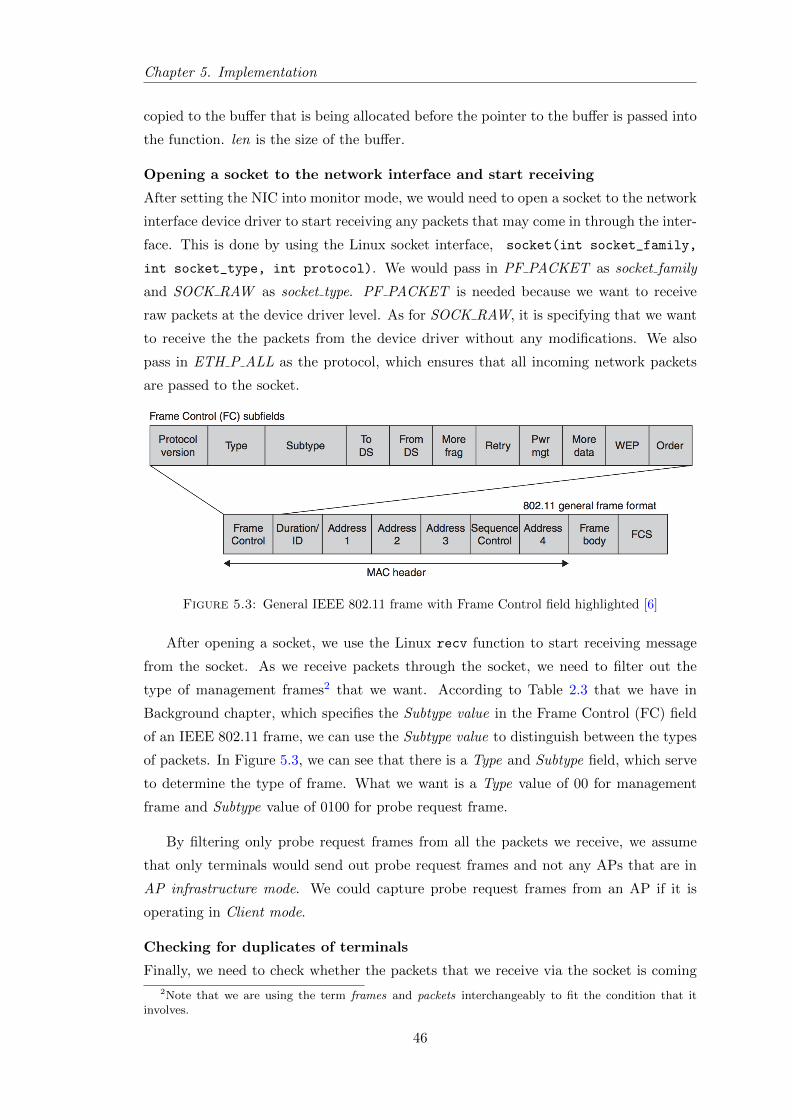
Chapter 5. Implementation
copied to the buffer that is being allocated before the pointer to the buffer is passed into
the function. len is the size of the buffer.
Opening a socket to the network interface and start receiving
After setting the NIC into monitor mode, we would need to open a socket to the network
interface device driver to start receiving any packets that may come in through the inter-
face. This is done by using the Linux socket interface, socket(int socket_family,
int socket_type, int protocol). We would pass in PF PACKET as socket family
and SOCK RAW as socket type. PF PACKET is needed because we want to receive
raw packets at the device driver level. As for SOCK RAW, it is specifying that we want
to receive the the packets from the device driver without any modifications. We also
pass in ETH P ALL as the protocol, which ensures that all incoming network packets
are passed to the socket.
Figure 5.3: General IEEE 802.11 frame with Frame Control field highlighted [6]
After opening a socket, we use the Linux recv function to start receiving message
from the socket. As we receive packets through the socket, we need to filter out the
type of management frames2 that we want. According to Table 2.3 that we have in
Background chapter, which specifies the Subtype value in the Frame Control (FC) field
of an IEEE 802.11 frame, we can use the Subtype value to distinguish between the types
of packets. In Figure 5.3, we can see that there is a Type and Subtype field, which serve
to determine the type of frame. What we want is a Type value of 00 for management
frame and Subtype value of 0100 for probe request frame.
By filtering only probe request frames from all the packets we receive, we assume
that only terminals would send out probe request frames and not any APs that are in
AP infrastructure mode. We could capture probe request frames from an AP if it is
operating in Client mode.
Checking for duplicates of terminals
Finally, we need to check whether the packets that we receive via the socket is coming
2Note that we are using the term frames and packets interchangeably to fit the condition that itinvolves.
46

Chapter 5. Implementation
from the same terminal or a different terminal. In Listing 5.2, it shows a hash function,
which is being used to check whether we have already pick up probe request frame from
the same terminal before.
12 int hashedValue = (mac[5] + (mac[4] << 8)) % MAX HOSTS;
Listing 5.2: A hash function.
Scanning different WiFi channels
Since we have learnt from Background that there are 13 channels allowed to be used in
Europe, we need to set the NIC to the channel we want to monitor for packets. This is
also done by using the function we have discussed earlier, wl_ioctl, using appropriate
identifier. Since we know that Channel 1, 3, 6, 8 and 11 provide a continuous overlapping
of all 13 channels as mentioned in Section 2.1.1 (Background), we could simply just
monitor for packets in each of these channels for a short period of time. This period
of time would be calibrated by some experimentations, which we discusses more in the
next paragraph.
Duration to monitor for packets
We need to decide on how long we want to monitor for packets that the NIC is receiving
before we transmit the collected data to the central server. We want to make sure that
this duration would provide sufficient time for the AP to capture any probe request
frames and detect any terminals that are nearby to it. After some experimentations
to find the optimal duration, it was found to be 30 seconds. Hence, our AP will scan
for any terminals nearby for 30 seconds before it transmit this information to a central
server for processing.
Saving MAC addresses and RSSI information of detected terminals
After we have collected information about the presence of terminals near an AP, we
need to save this data to a file for transmission to a central server. How we are going to
serialise the data before transmission and how we are transferring it would be discussed
in Section 5.2.2 and 5.2.4 below.
Since we decide to use a file transmission library to handle the transferring of data
from AP to server, we would need to store the data to a file locally first. After exper-
imentation with DD-WRT, we discover that it is possible to store file in the directory
/tmp, which actually uses up the RAM of the AP for storing the file. Once the AP is
restarted, the file will be gone. This is quite an interesting discovery in that DD-WRT
seems to mount the /tmp directory using an area of the RAM. Since we also know that
re-writing too many times on JFFS filesystem3 would eventually damage the embedded
3To write to JFFS filesystem, we can save a file to the directory /jffs.
47

Chapter 5. Implementation
device’s flash storage space, it would be better to store our file using the space on the
RAM in /tmp directory. This actually fits our purpose directly since we are only keeping
the file temporarily. We will overwrite over the file after every 30 seconds of scanning
and completing transmission of the data file to the central server.
5.2.2 Data Serialisation
Since we need to transfer data, containing detected MAC addresses and its associated
RSSI, from the AP to a server, we need to find an efficient way of serialising the data
so that the serialised data is still small and secure for transfer.
Selecting a serialisation method
We have outlined the advantages and disadvantages of each available serialisation method
that we could use for our project. We would like to briefly justify our final choice. Using
tab-delimited to store our data is not very space efficient. Furthermore, this method of
using tab to separate values requires us to use string functions extensively to concatenate
values, which is computationally expensive and is not that fast as compared to some-
thing like Protocol Buffers. Protocol buffers provide a very fast parser for deserialising
the data from raw bytes. As for JSON format, it takes too much space to store the key
for each of its associated values. In contrast, Protocol Buffers do not need any key as-
sociated to a value in order to interpret the data. It simply uses an Interface Definition
Language (IDL) file, which serves as a template for deserialising the data. In addition,
there is a C-implementation of Protocol Buffers for embedded device, Nanopb, which we
can use to serialise data on the AP and use the Java implementation of Protocol Buffers
from Google on the processing server to deserialise the data.
The reason why we want to choose a serialisation method that results in a smaller
serialised data is because we want to save the bandwidth of transferring the data from
AP to server. This is even more relevant since our AP is sending data every 30 seconds,
which means that we should try to reduce the amount of data to be transmitted as much
as possible. As long as the AP could handle the serialisation process without requiring
too much computing resources, we could employ a more efficient serialisation method
like Protocol Buffers.
Defining Protocol Buffer IDL
An IDL file has an extension .proto. In Listing 5.3, we have shown how we choose
to define the structure of how we are going to send the collected data. ClientType is
a message type, which encapsulates the detail of each individual terminal, namely its
MAC address and RSSI value. Since MAC address is made up of 48 bits, we choose
to store it in hexadecimal, which takes only 6 bytes for each terminal we have. This
48
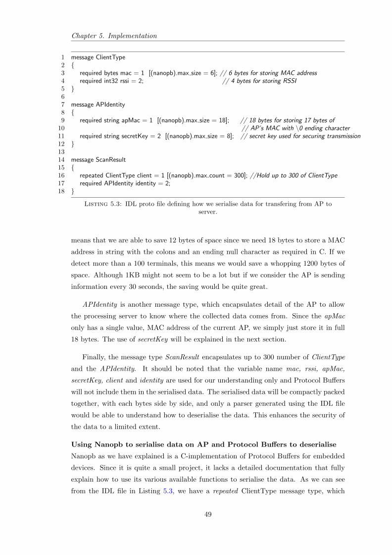
Chapter 5. Implementation
1 message ClientType2 {3 required bytes mac = 1 [(nanopb).max size = 6]; // 6 bytes for storing MAC address4 required int32 rssi = 2; // 4 bytes for storing RSSI5 }67 message APIdentity8 {9 required string apMac = 1 [(nanopb).max size = 18]; // 18 bytes for storing 17 bytes of
10 // AP’s MAC with \0 ending character11 required string secretKey = 2 [(nanopb).max size = 8]; // secret key used for securing transmission12 }1314 message ScanResult15 {16 repeated ClientType client = 1 [(nanopb).max count = 300]; //Hold up to 300 of ClientType17 required APIdentity identity = 2;18 }
Listing 5.3: IDL proto file defining how we serialise data for transfering from AP toserver.
means that we are able to save 12 bytes of space since we need 18 bytes to store a MAC
address in string with the colons and an ending null character as required in C. If we
detect more than a 100 terminals, this means we would save a whopping 1200 bytes of
space. Although 1KB might not seem to be a lot but if we consider the AP is sending
information every 30 seconds, the saving would be quite great.
APIdentity is another message type, which encapsulates detail of the AP to allow
the processing server to know where the collected data comes from. Since the apMac
only has a single value, MAC address of the current AP, we simply just store it in full
18 bytes. The use of secretKey will be explained in the next section.
Finally, the message type ScanResult encapsulates up to 300 number of ClientType
and the APIdentity. It should be noted that the variable name mac, rssi, apMac,
secretKey, client and identity are used for our understanding only and Protocol Buffers
will not include them in the serialised data. The serialised data will be compactly packed
together, with each bytes side by side, and only a parser generated using the IDL file
would be able to understand how to deserialise the data. This enhances the security of
the data to a limited extent.
Using Nanopb to serialise data on AP and Protocol Buffers to deserialise
Nanopb as we have explained is a C-implementation of Protocol Buffers for embedded
devices. Since it is quite a small project, it lacks a detailed documentation that fully
explain how to use its various available functions to serialise the data. As we can see
from the IDL file in Listing 5.3, we have a repeated ClientType message type, which
49

Chapter 5. Implementation
requires a different way of putting the message into ScanResult multiple times. Hence,
we have to spend quite a great deal of time experimenting on how to write an encoding
function to serialise this type of message. However, it is worth the time to get it to work
because Nanopb is extremely fast in serialising data due to its optimisation with only
essential features for embedded devices.
After serialising, deserialising would have to take place. However, this time round, it
happens on the server side. We use the same IDL proto file to feed into Google Protocol
Buffer generator to generate a parser. The parser allows us to deserialise the data and
retrieve the pieces of information we want.
5.2.3 Securing Transmission
One of the major concerns that we, as software engineers, have is security. If a
system is designed without security in mind, one day, it will be susceptible to attacks
by rogue users. Hence, even though our project is only a prototype, we would like to
add one layer of security into the prototype at this stage.
In order to prevent rogue APs that does not belong to us from sending garbage data
to the central Processing Agent, we introduced something called secret key. Only APs
that belong to us would know about this secret key and as you can see in Listing 5.3,
the secret key will be serialised using the Protocol Buffers. Since it might be slightly
hard to deserialise the raw bytes without having the IDL proto file, the secret key would
appear just like any other kinds of data. Thus, it is not easy for someone to know that
it is a secret key. When we are receiving the serialised data at the Processing Agent, we
would deserialise it and compare the secret key with the one we have on the Processing
Agent. Hence, this forms the basic level of security.
If we want to make sure that hackers would not be able to obtain the secret key from
the serialised data at all, we could use a HTTPS connection for encrypting the data to
be transmitted between AP and server.
5.2.4 File Transmission
After we have serialised the data at the AP, we need to decide on a way to transfer
this data to the Processing Agent. We would have a pre-condition for this, i.e., the
AP need to have an internet connectivity or be connected to a private network with a
Processing Agent on the network. We will discuss more about Processing Agent later in
Section 5.3. As for now, we would like to focus on the various ways that we can employ
to transfer data from an AP to a server.
50
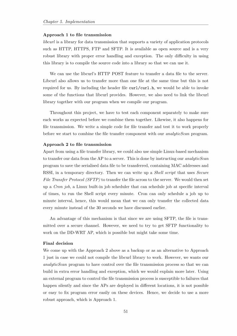
Chapter 5. Implementation
Approach 1 to file transmission
libcurl is a library for data transmission that supports a variety of application protocols
such as HTTP, HTTPS, FTP and SFTP. It is available as open source and is a very
robust library with proper error handling and exception. The only difficulty in using
this library is to compile the source code into a library so that we can use it.
We can use the libcurl’s HTTP POST feature to transfer a data file to the server.
Libcurl also allows us to transfer more than one file at the same time but this is not
required for us. By including the header file curl/curl.h, we would be able to invoke
some of the functions that libcurl provides. However, we also need to link the libcurl
library together with our program when we compile our program.
Throughout this project, we have to test each component separately to make sure
each works as expected before we combine them together. Likewise, it also happens for
file transmission. We write a simple code for file transfer and test it to work properly
before we start to combine the file transfer component with our analyticScan program.
Approach 2 to file transmission
Apart from using a file transfer library, we could also use simple Linux-based mechanism
to transfer our data from the AP to a server. This is done by instructing our analyticScan
program to save the serialised data file to be transferred, containing MAC addresses and
RSSI, in a temporary directory. Then we can write up a Shell script that uses Secure
File Transfer Protocol (SFTP) to transfer the file across to the server. We would then set
up a Cron job, a Linux built-in job scheduler that can schedule job at specific interval
of times, to run the Shell script every minute. Cron can only schedule a job up to
minute interval, hence, this would mean that we can only transfer the collected data
every minute instead of the 30 seconds we have discussed earlier.
An advantage of this mechanism is that since we are using SFTP, the file is trans-
mitted over a secure channel. However, we need to try to get SFTP functionality to
work on the DD-WRT AP, which is possible but might take some time.
Final decision
We come up with the Approach 2 above as a backup or as an alternative to Approach
1 just in case we could not compile the libcurl library to work. However, we wants our
analyticScan program to have control over the file transmission process so that we can
build in extra error handling and exception, which we would explain more later. Using
an external program to control the file transmission process is susceptible to failures that
happen silently and since the APs are deployed in different locations, it is not possible
or easy to fix program error easily on these devices. Hence, we decide to use a more
robust approach, which is Approach 1.
51
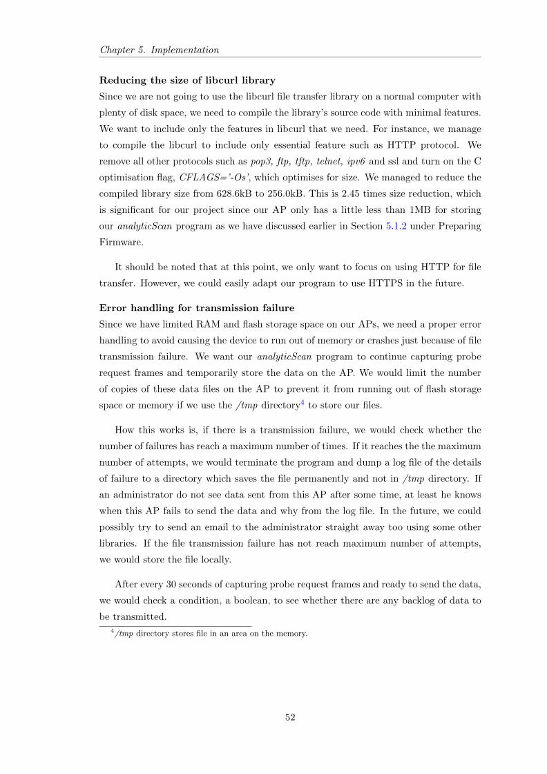
Chapter 5. Implementation
Reducing the size of libcurl library
Since we are not going to use the libcurl file transfer library on a normal computer with
plenty of disk space, we need to compile the library’s source code with minimal features.
We want to include only the features in libcurl that we need. For instance, we manage
to compile the libcurl to include only essential feature such as HTTP protocol. We
remove all other protocols such as pop3, ftp, tftp, telnet, ipv6 and ssl and turn on the C
optimisation flag, CFLAGS=’-Os’, which optimises for size. We managed to reduce the
compiled library size from 628.6kB to 256.0kB. This is 2.45 times size reduction, which
is significant for our project since our AP only has a little less than 1MB for storing
our analyticScan program as we have discussed earlier in Section 5.1.2 under Preparing
Firmware.
It should be noted that at this point, we only want to focus on using HTTP for file
transfer. However, we could easily adapt our program to use HTTPS in the future.
Error handling for transmission failure
Since we have limited RAM and flash storage space on our APs, we need a proper error
handling to avoid causing the device to run out of memory or crashes just because of file
transmission failure. We want our analyticScan program to continue capturing probe
request frames and temporarily store the data on the AP. We would limit the number
of copies of these data files on the AP to prevent it from running out of flash storage
space or memory if we use the /tmp directory4 to store our files.
How this works is, if there is a transmission failure, we would check whether the
number of failures has reach a maximum number of times. If it reaches the the maximum
number of attempts, we would terminate the program and dump a log file of the details
of failure to a directory which saves the file permanently and not in /tmp directory. If
an administrator do not see data sent from this AP after some time, at least he knows
when this AP fails to send the data and why from the log file. In the future, we could
possibly try to send an email to the administrator straight away too using some other
libraries. If the file transmission failure has not reach maximum number of attempts,
we would store the file locally.
After every 30 seconds of capturing probe request frames and ready to send the data,
we would check a condition, a boolean, to see whether there are any backlog of data to
be transmitted.
4/tmp directory stores file in an area on the memory.
52
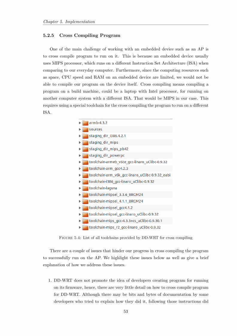
Chapter 5. Implementation
5.2.5 Cross Compiling Program
One of the main challenge of working with an embedded device such as an AP is
to cross compile program to run on it. This is because an embedded device usually
uses MIPS processor, which runs on a different Instruction Set Architecture (ISA) when
comparing to our everyday computer. Furthermore, since the computing resources such
as space, CPU speed and RAM on an embedded device are limited, we would not be
able to compile our program on the device itself. Cross compiling means compiling a
program on a build machine, could be a laptop with Intel processor, for running on
another computer system with a different ISA. That would be MIPS in our case. This
requires using a special toolchain for the cross compiling the program to run on a different
ISA.
Figure 5.4: List of all toolchains provided by DD-WRT for cross compiling
There are a couple of issues that hinder our progress in cross compiling the program
to successfully run on the AP. We highlight these issues below as well as give a brief
explanation of how we address these issues.
1. DD-WRT does not promote the idea of developers creating program for running
on its firmware, hence, there are very little detail on how to cross compile program
for DD-WRT. Although there may be bits and bytes of documentation by some
developers who tried to explain how they did it, following those instructions did
53

Chapter 5. Implementation
not always work for us. There are always problems here and there during the
compilation when we follow others’ instruction because their machine and ours
are usually not running the same types and version of OS. Furthermore, the other
developers’ machine may have some magical libraries that are required to make
the cross compilation work but we may not have them.
2. From Figure 5.4, we can see that there are 17 different toolchains provided by
DD-WRT. Out of these 17 toolchains, there are 8 with the name mips in them.
No matter how hard we try to find an answer online, we could not find the correct
answer as to which toolchain to use. Hence, we have to experiment with compiling
our program one by one and try to run it on the AP. The hardest part is, since
our program uses some third-party and kernel libraries provided by the firmware,
we are not sure whether a particular feature that is not working is because of
cross compiling problem or there is something wrong with the libraries. Hence, we
decide to focus on trying out each toolchain on compiling a file transmission test
program to see whether cross compiling a program using a third-party library is
working.
3. Just like what we have mentioned in the previous bullet points, we need to use
other libraries, which could be dynamic libraries (end with .so extension) or static
libraries (end with .a extension). If we compile our program using dynamic li-
braries, we need to share this libraries with other programs too and if these li-
braries are not available at program run-time, the functions provided by these
libraries will not work. If we compile our program using static libraries, these
libraries would be statically linked by the linker into the final executable of our
program. This would increase the size of the program.
However, the problem now is we need to find out how we can get the dynamic
or static libraries that we need. This is achieved by downloading the whole source
of DD-WRT, which is over 18GB in size, and attempt to cross compile the whole
firmware to generate the libraries that we need to use. This process is challenging
but also fun at the end when we are able to accomplish it. We believe not many
people are able to cross compile the firmware as there are too many dependencies
and issues to fix during the compilation process.
4. Another issue that we face is also the version of Linux kernel that we need to
include in our Makefile since we also call some of the functions provided by the
kernel. Hence, we have to test a few versions of the kernel as well.
In Figure 5.5, we have illustrated the whole compilation process. At the top of the
diagram, we started off by cross compiling DD-WRT source code and libcurl source
code to get the libraries that we need. Then, we cross compile our program and link
54
Chapter 5. Implementation
Figure 5.5: The Cross Compiling process
Figure 5.6: Detail of the generated executable binary program file
the libraries with it. This generate an executable binary file, which we can transfer by
Secure Copy (SCP) to the AP for executing. In Figure 5.6, it shows the detail of the
executable binary file that we have generated. LSB means Least Significant Byte.
Means of transferring our program to AP
Finally, we would like to mention that since we are able to configure the AP to support
SSH, we are able to use SCP to transfer our executable binary file to the AP. Initially,
before we use SCP, we also try other alternatives such as uploading the binary file onto
a server connected to the internet and use the Linux program wget to download the
program back from the server since the AP has internet connectivity. However, we know
that this is just a quick and dirty way and we use it initially because we are excited to
test our compiled program on the AP. After that, we always use SCP for file transfer to
the AP, which is much more convenient.
55

Chapter 5. Implementation
5.3 Building a Processing Agent
After we have completed the lower stack of our system, we need to implement the
higher level modules to manage the data that is transmitted from the AP and attempt
to process them. Ultimately, we want to convert the raw data that we have collected to
something insightful and useful. In this section, we will explain how we implement the
Processing Agent, which is a server with Java web servlet deployed using Tomcat5.
5.3.1 Initialising Web Servlet
We want our servlet to respond to HTTP GET or POST request, hence, our
ProcessingAgent class extends the HttpServlet. The ProcessingAgent class is the
main servlet class that we have configured in a web.xml setting file to point to. This
means that any HTTP GET or POST request to a url like http://localhost/ProcessingAgent
would be directed to the ProcessingAgent servlet to handle.
When a servlet is created after we start Tomcat, the method init() will be invoked.
Likewise when Tomcat is stopped, the method destroy() will be invoked. Since we are
using HBase as our database choice, which we will explain more on it later, we need to
create a pool of connections to the database that is available for usage when we want to
transmit data to it. We will create this pool within the init() method and close any
connections in the destroy() method. The pool of connections is needed because it is
quite expensive to always having to set up a new connection to the database everytime
each AP send in some data. However, having learnt that the HBase connections in the
pool may become unusable after a long period of time, we choose to refresh6 the pool
every 3 hours. A Check logic has been implemented for this, which checks that if the
pool has been established for 3 hours, we will refresh it.
5.3.2 Receiving and Deserialising Data
An HTTP request could be a GET or a POST. We implement two methods doGet()
and doPost(), which override the existing methods in HttpServlet. Any HTTP GET
request will invoke the doGet() method and any HTTP POST request will invoke the
doPost() method.
5Tomcat is an open source web server that host a Java servlet.6When we refresh the pool, we mean closing all existing connections in the pool and opening new
ones and put back into the pool so that any instances of object could use the connection.
56
Chapter 5. Implementation
In order to receive file from a remote end via HTTP, we use the ServletFileUpload
class that is available in the org.apache.commons.fileupload.servlet.ServletFileUpload
package. We could then retrieve the content of the file being uploaded from the InputStream.
Apart from receiving the data, we also need to deserialise it. We use the Google
Protocol Buffers generator together with our IDL proto template file to generate a
parser, which also provides accessor methods for retrieving each of the information that
we have serialised. One of the main concern that we have is how do we know how big
is the data that is being uploaded by the AP so that we can allocate the right amount
of memory space to hold it. This is because we do not want to store the data as a file
first before we pass the file to the Protocol Buffer parser. However, it appears that we
are able to pass the InputStream that is used to receive the data straight to the parser.
Hence, there is no intermediate storing of temporary file before we parse the content of
the file.
Checking authenticity of sender
After we deserialise the data, we would check the secret key that we have packed with
the other kinds of data (MAC addresses and RSSI). We compare the secret key with
the one we store on the Processing Agent to make sure the data sent from the AP is
authentic.
5.3.3 Adding Timestamp
We want the time from all APs to be synchronised and agree with each other. If one
AP’s time is 5 minutes faster than another AP’s time, then this will affect our aggregation
of data very seriously. This is because we need to insert a timestamp for each record,
which is make up of terminal’s MAC address, RSSI and the AP MAC address that
detects the terminal. We need the timestamp during the aggregation stage to determine
at what time a terminal leaves a particular area. This is just one of the aggregations
that uses timestamp. We will explain more later in Section 5.5 on aggregating data.
There are two approaches to inserting timestamp and they are discussed below.
Approach 1 to adding timestamp
We can add a timestamp to each record at the AP using the AP’s time. However, this
would mean that we need to carry out clock sychronisation of the AP every now and
then. We may use the Linux program ntptime which provides Network Time Protocol to
sychronise computer clock. This program is available on the DD-WRT firmware but is
unusable. After our testing, we discover that it is not possible to use it to synchronise or
even set the AP’s clock time. There appears to be some bugs with the ntptime program
on DD-WRT firmware.
57
Chapter 5. Implementation
Approach 2 to adding timestamp
We can add the timestamp to each record at the Processing Agent using the server’s
clock time. This would provide an accurate timestamp for all the records. Even if we
are going to deploy more than one Processing Agent by using load balancing solution,
we could still sychronise the servers’ clock time more easily than the APs’ clock time.
There is one problem associated with this mechanism, that is, if there is any delay
in the transfer of data from the AP to the agent, this would be a problem. However,
we just want the timestamp of each records from different APs to agree with each other
and not too particular about the precision. Previously, we have mentioned that we are
going to retry file transmission up to a limit if the current transfer attempt fails. We
do recognise that this is another case to address because if a file fails to be transmitted
from an AP to the agent and after some time of retries, it succeed, the timestamp we
are adding for the record would not be correct anymore.
Final decision
We have seen above that each approach has its advantages and disadvantages. However,
for Approach 1, since DD-WRT does not allow us to set the clock of the AP to a correct
time, Approach 1 would be ruled out completely. Hence, we are left with Approach
2. Although the case of failed transmission may cause the timestamp to be wrong, we
know that it would not always be the case that our AP loses network connectivity to
the Processing Agent and ends up with failed file transmission. Therefore, Approach 2
is the best choice that we can follow for now.
If we have more time to work on this, we could actually insert a notice (a time
counter) at the AP for each of the files that fail to transmit and we can use the time
counter to determine the actual time of each file. For example, if file1, file2 and file3
fail to be sent in this sequence, we will insert a time counter of 3, 2 and 1 to each file
respectively. When we receive each file at the Processing Agent, we would check the
time counter parameter. If it is 3, we will adjust the timestamp for all records from file1
to 30s * 3, i.e., the actual timestamp for file1 is 90s ago. This assumes that file1 is the
first that is failed to be transmitted and file3 is the last.
Format of timestamp
We choose to use the Unix time7, also known as POSIX time, as the format of our
timestamp. This format is more reliable and is not susceptible to the problem of different
timezones or daylight saving. In this project, we noticed that if we did not use Unix
time format, the British Summer Time change would affect our timestamp if we stored
7Unix time is defined as the number of seconds that have elapsed since 00:00:00 Coordinated UniversalTime (UTC), 1 January 1970[31]
58

Chapter 5. Implementation
it in the normal date format (DDMMYYYY HH:mm:ss). With the timestamp in Unix
time format, Java would be able to interpret the correct time based on the timezone the
server uses.
5.3.4 Pushing Data to Database
Finally, pushing the data to the database is the final stage on the Processing Agent.
We push a record for each terminal that our AP has detected to the database. A
detection record is defined as follows:
AP MAC address Terminal MAC address RSSI Timestamp
Table 5.1: A Record
In Table 5.1, the AP MAC is the MAC address of the AP, which has detected that
particular WiFi terminal. From now on, we shall refer to a detection record as having
the structure above so that it is easier for us to explain about the aggregation process
later on.
5.4 Storing and Managing Data
There are many ways that we can store data, but finding the best possible way to
store it so that it fits our data access pattern requires some analysis. In our original
objective, we want to find a database that is massively scalable to handle the continuous
stream of data from all APs, we want to have flexible data types and schema and we
do not need the time critical transaction feature of relational database. This is because
we are not talking about high frequency trading in Banks, in which each of the trade
orders need to observe strict consistency. In order to maintain strict consistency, the
database management system would have to sacrifice read and write performance of
data. Hence, since we do not need such feature, it is clear that we should try out the
next generation database, NoSQL, which becomes more and more popular recently due
to the emergence of different NoSQL databases such as HBase, CouchDB, MongoDB
and Cassandra. NoSQL has very fast write performance, which is good for us to push in
more data simultaneously collected from each AP. Even if we have a thousand of APs,
this would be no sweat for NoSQL database.
The best thing that these NoSQL solution provides would be their tight integration
with MapReduce, which is a powerful framework to process huge amount of data in
parallel and across many machines. An alternative to MapReduce would be to use the
Online analytical processing (OLAP) feature of relational database. However, this work
59
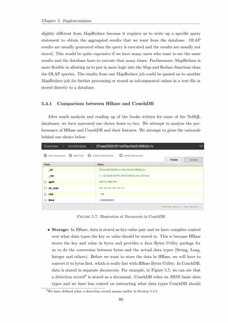
Chapter 5. Implementation
slightly different from MapReduce because it requires us to write up a specific query
statement to obtain the aggregated results that we want from the database. OLAP
results are usually generated when the query is executed and the results are usually not
stored. This would be quite expensive if we have many users who want to see the same
results and the database have to execute that many times. Furthermore, MapReduce is
more flexible in allowing us to put in more logic into the Map and Reduce functions than
the OLAP queries. The results from one MapReduce job could be passed on to another
MapReduce job for further processing or stored as tab-separated values in a text file or
stored directly to a database.
5.4.1 Comparison between HBase and CouchDB
After much analysis and reading up of the books written for some of the NoSQL
databases, we have narrowed our choice down to two. We attempt to analyse the per-
formance of HBase and CouchDB and their features. We attempt to gives the rationale
behind our choice below:
Figure 5.7: Illustration of Documents in CouchDB
• Storage: In HBase, data is stored as key-value pair and we have complete control
over what data types the key or value should be stored in. This is because HBase
stores the key and value in bytes and provides a Java Bytes Utility package for
us to do the conversion between bytes and the actual data types (String, Long,
Integer and others). Before we want to store the data in HBase, we will have to
convert it to bytes first, which is really fast with HBase Bytes Utility. In CouchDB,
data is stored in separate documents. For example, in Figure 5.7, we can see that
a detection record8 is stored as a document. CouchDB relies on JSON basic data
types and we have less control on instructing what data types CouchDB should
8We have defined what a detection record means earlier in Section 5.3.4
60

Chapter 5. Implementation
store for each value. In HBase, each detection record can be stored as a row with
multiple columns.
• Access: Data can be inserted into HBase using its Java Client package, which
uses Remote Procedure Call (RPC) in its implementation. However, CouchDB
allows us to insert data into the database by using HTTP via its REST API.
Using HTTP is a little slower and is not that efficient.
• MapReduce: HBase allows us to chain multiple MapReduce jobs, i.e., the result
from the first MapReduce job can be passed as an input to the second MapReduce
job. However, CouchDB has a built-in MapReduce feature, which allows only one
job to be executed. Usually, we require executing a few MapReduce jobs to achieve
a final aggregated results that we want.
Figure 5.8: Storage size for 12817 Documents in CouchDB
Figure 5.9: Storage size for 5181 rows in HBase
Storage size comparison
In Figure 5.8, we can see that for 12817 documents, each storing a detection record with
details shown in Figure 5.7, the total size that is used is 10.2 MB. This is about 834
bytes per detection record. In Figure 5.9, we have attempted to use the HBase facility
to print out all values of each row and we can see that for 5181 rows, only 1.3 MB is
required for storing those rows. This is about 263 bytes per detection record. This is
3.17 times better than how CouchDB stores the data. The reason behind this is that
61

Chapter 5. Implementation
CouchDB has a few extra metadata, which uses up quite a bit of space and CouchDB
does not allow us to control the data types of the value being stored.
Although we have make use of Restlet, a REST client library, to implement the
mechanism to push data into CouchDB from the Processing Agent, we choose to abandon
the code we have written in favour of using HBase.
5.4.2 Setting up of HBase, HDFS, MapReduce and Zookeeper
Setting up HBase is time consuming and with a level of uncertainty. This is because
most of HBase users are corporate users such as Facebook, StumbleUpon and Twitter,
and these companies have active development teams to setup, maintain and write their
applications to make use of HBase. If there are more ordinary users, there would be more
documentations and instructions shared by other users like us. Hence, a large portion
of our time was also spent on setting HBase, HDFS, MapReduce and Zookeeper. Since
HBase makes use of Hadoop Distributed Filesystem for storing its data, it also can
make use of Hadoop MapReduce functionality. We also need to install a Zookeeper, a
distributed coordination service, which is required as part of HBase deployment.
We attempt to use the Cloudera distribution9 for the installation of HBase and other
components. However, even using Cloudera distribution and following its instruction,
we still could not get HBase to work due to a number of problems, which take us a long
time to fix. We have briefly summarised these problems below.
• Incompatible Versions: Since HBase requires a few other components of Hadoop
to be installed, there are incompatible versions. To make things worst, since we
needed to use Hadoop and HBase Java client packages, some versions of the client
packages are not compatible with the version of Hadoop and HBase server compo-
nents. Although we installed HBase 0.94.2 on the server, its associated Java client
package version 0.94.2 is not compatible with it. After we wrote our MapReduce
code making use of the Java client package version 0.94.2, the execution throws
a weird exception, which we could not understand and searching through the in-
ternet yield minimal help. It took us a long time before we realised that using an
older version of the HBase Java client package 0.92.1 works with the HBase server
0.94.2. We have raised this issue to the HBase development community.
• Heap size: Since HBase is built for massive scalability, its memory requirement
is huge as well. For HDFS, there are a few different components such as Datanode
and Namenode. Within HBase, there are Hbase Master, Hbase RegionServer and
REST server. There are also MapReduce TaskTracker and JobTracker as well
9Cloudera provides hosting of some HBase and Hadoop versions that we can download and install.
62

Chapter 5. Implementation
as Zookeeper. Since we choose to setup HBase and Hadoop in Pseudo-distributed
Mode for this project, the whole setup requires huge amount of memory on a single
server. In Pseudo-distributed Mode, each of the components we have mentioned
would exist as a separate process on the computer system. We need to find the dif-
ferent configuration files, which are located in many different locations, to alter the
JVM Max Heap size allowance to limit the amount of memory each process uses.
We also have to decide on a value that would not cause some of the components
to run out of memory.
• IpV6: Currently, HBase is reported to cause some issues with IpV6. We discovered
this after our code threw up some exceptions and we found out that it was related
to IpV6. Hence, we disable the IpV6 support in CentOS, which is the Linux OS
we use for our HBase setup.
• Reverse DNS Lookup: HBase requires that we properly configure the Reverse
DNS Lookup in order for it to function properly.
5.4.3 Data Schema Design
packet detailsap mac terminal mac rssi timestamp
row key1 01:02:03:04:05:06 22:22:22:AS:BB:CC -65 1369908231
row key2 ... ... ... ...
row key3 ... ... ... ...
Table 5.2: HBase Table Structure for Detection Records10
Although HBase is flexible on schema, we still need to know how we define our row
key, so that it allows us to query for our data. Designing a good row key structure is
very important in HBase. This is because it will provide ease of access to the data that
we want and for performance purposes. We have reproduced the same table example
that we have given in Chapter 2 (Background) so that we can easily refer to it in this
chapter. In Table 5.2, row key1 is a row key, packet details is a column family and
ap mac, terminal mac, rssi and timestamp are column qualifiers. ap mac is the MAC
address of the AP, which detects the terminal. terminal mac is the MAC address of the
terminal being detected. rssi is the received signal strength. timestamp gives the time
at which the AP detects the terminal.
We have explained before in Background that HBase might store column families
on different RegionServers (servers that host small chunks of HBase table) for high
availability and scaling purposes. However, HBase also relies on the row key to decide
which rows go to which RegionServers. Hence, if we do not design a good row key, this
may affect the performance of data read and write.
63

Chapter 5. Implementation
Figure 5.10: Balance between sequential read and write performance [18]
In Figure 5.10, sequential key refers to a row key that follows a sequence such as
1,2,3 ... 100. Random key refers to a key that is generated randomly. Using a sequential
key, it would be faster for us to select detection records that fall within a range of time.
We have defined our row key to have the following structure.
〈cluster id〉 − 〈timestamp〉 − 〈ap mac〉 − 〈incremental count〉
The row key shown above is a composite row key, which is make up of different pieces
of information that we combine together for ease of querying the row from the table. It
should be noted that the precedence increases from left to right. We design the key this
way with consideration of the way we are going to select a range of rows for input to
MapReduce jobs later. We provide explanations for the row key design below:
• cluster id We may have many clusters of APs deployed in different location, for
example, 20 APs in Shopping Mall 1 and 30 APs in Shopping Mall 2 and 50 APs in
Shopping Mall 3. The cluster id would serves to segregate the records that belong
to different clusters.
• timestamp Next, we have the timestamp. HBase provides a feature to scan for
a range of rows in order to fetch them. The timestamp contributes the sequential
portion of the key so that we can specify a scan start key and a scan end key to
select rows that have their timestamp portion of the key falling in between the
start and end key. We will explain this more later as we start explaining about
our aggregation logic.
• ap mac As for ap mac, we want to include it in the row key so that we know
which AP the particular record belongs to.
64
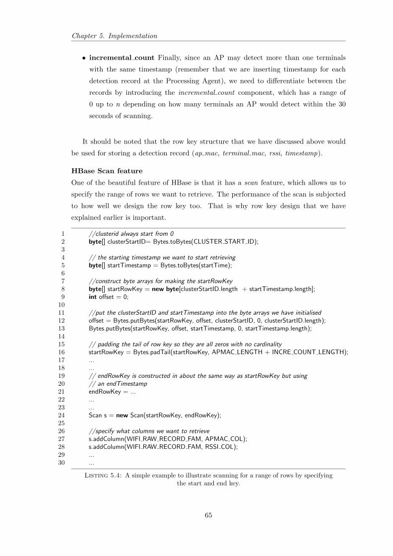
Chapter 5. Implementation
• incremental count Finally, since an AP may detect more than one terminals
with the same timestamp (remember that we are inserting timestamp for each
detection record at the Processing Agent), we need to differentiate between the
records by introducing the incremental count component, which has a range of
0 up to n depending on how many terminals an AP would detect within the 30
seconds of scanning.
It should be noted that the row key structure that we have discussed above would
be used for storing a detection record (ap mac, terminal mac, rssi, timestamp).
HBase Scan feature
One of the beautiful feature of HBase is that it has a scan feature, which allows us to
specify the range of rows we want to retrieve. The performance of the scan is subjected
to how well we design the row key too. That is why row key design that we have
explained earlier is important.
1 //clusterid always start from 02 byte[] clusterStartID= Bytes.toBytes(CLUSTER START ID);34 // the starting timestamp we want to start retrieving5 byte[] startTimestamp = Bytes.toBytes(startTime);67 //construct byte arrays for making the startRowKey8 byte[] startRowKey = new byte[clusterStartID.length + startTimestamp.length];9 int offset = 0;
1011 //put the clusterStartID and startTimestamp into the byte arrays we have initialised12 offset = Bytes.putBytes(startRowKey, offset, clusterStartID, 0, clusterStartID.length);13 Bytes.putBytes(startRowKey, offset, startTimestamp, 0, startTimestamp.length);1415 // padding the tail of row key so they are all zeros with no cardinality16 startRowKey = Bytes.padTail(startRowKey, APMAC LENGTH + INCRE COUNT LENGTH);17 ...18 ...19 // endRowKey is constructed in about the same way as startRowKey but using20 // an endTimestamp21 endRowKey = ...22 ...23 ...24 Scan s = new Scan(startRowKey, endRowKey);2526 //specify what columns we want to retrieve27 s.addColumn(WIFI RAW RECORD FAM, APMAC COL);28 s.addColumn(WIFI RAW RECORD FAM, RSSI COL);29 ...30 ...
Listing 5.4: A simple example to illustrate scanning for a range of rows by specifyingthe start and end key.
65

Chapter 5. Implementation
In Listing 5.4, we have shown an example of how we construct the start and end
row key in order to retrieve the range of rows that we want. This is important because
if we want to aggregate records that fall between 10AM and 2PM of today , we would
use the Unix time format of 10AM (1371117600) as the startTime and that of 2PM
(1371132000) as the endTime. Since we have chosen to include the timestamp in the
row key structure, this would allow us to retrieve the detection records that fall within
this range for aggregation simply by creating the scan object like the one we have in
Listing 5.4.
From Listing 5.4, we can see that we pad the tail of the rest of the row key on Line
16. This means that only the cluster id and timestamp would take precedence.
5.5 Aggregating Data
In this section, we will explain the logic behind our MapReduce functions, which are
powerful in localising a terminal, counting the number of terminals near each AP and
tracking how long each terminal stays near an AP. The great thing about using Hadoop
MapReduce together with HBase is the native support from HBase for MapReduce.
This is because HBase’s data is stored on HDFS in a distributed fashion, hence, the
MapReduce component of Hadoop can also be carried out on the HBase’s data in parallel.
The good thing about this is that we can use data that is stored in HBase’s table as
both the source and as a sink. We can specify which table will provide the data as the
input of the Map function and which table will be responsible for storing the output
results from the Reduce function. The scan feature that we have discussed earlier is
extremely useful here for MapReduce. It allows us to specify which range of rows we
want to retrieve and pass as input to the Map function.
1 import org.apache.hadoop.hbase.mapreduce.TableMapReduceUtil;2 import org.apache.hadoop.hbase.mapreduce.TableMapper;3 import org.apache.hadoop.hbase.mapreduce.TableReducer;4 ...5 ...6 TableMapReduceUtil.initTableMapperJob(WIFI TABLE NAME, scan, Mapper1.class,7 ImmutableBytesWritable.class, Put.class, job);8 TableMapReduceUtil.initTableReducerJob(WIFI AGGRE TABLE NAME, Reducer1.class, job);9 ...
Listing 5.5: Importing relevant packages and setup MapReduce jobs.
In Listing 5.5, it shows the packages that we need to import in Java in order to use
the Hadoop MapReduce with HBase’s table, in which we create to store data.
66
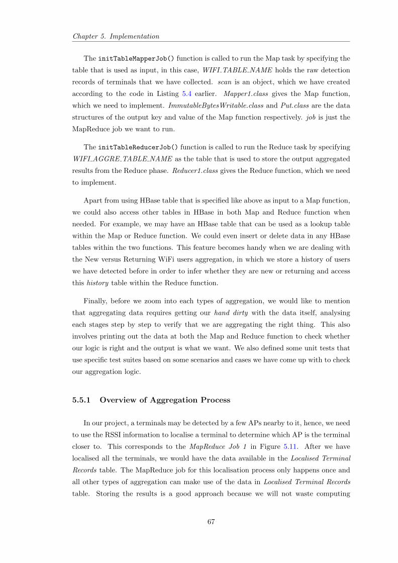
Chapter 5. Implementation
The initTableMapperJob() function is called to run the Map task by specifying the
table that is used as input, in this case, WIFI TABLE NAME holds the raw detection
records of terminals that we have collected. scan is an object, which we have created
according to the code in Listing 5.4 earlier. Mapper1.class gives the Map function,
which we need to implement. ImmutableBytesWritable.class and Put.class are the data
structures of the output key and value of the Map function respectively. job is just the
MapReduce job we want to run.
The initTableReducerJob() function is called to run the Reduce task by specifying
WIFI AGGRE TABLE NAME as the table that is used to store the output aggregated
results from the Reduce phase. Reducer1.class gives the Reduce function, which we need
to implement.
Apart from using HBase table that is specified like above as input to a Map function,
we could also access other tables in HBase in both Map and Reduce function when
needed. For example, we may have an HBase table that can be used as a lookup table
within the Map or Reduce function. We could even insert or delete data in any HBase
tables within the two functions. This feature becomes handy when we are dealing with
the New versus Returning WiFi users aggregation, in which we store a history of users
we have detected before in order to infer whether they are new or returning and access
this history table within the Reduce function.
Finally, before we zoom into each types of aggregation, we would like to mention
that aggregating data requires getting our hand dirty with the data itself, analysing
each stages step by step to verify that we are aggregating the right thing. This also
involves printing out the data at both the Map and Reduce function to check whether
our logic is right and the output is what we want. We also defined some unit tests that
use specific test suites based on some scenarios and cases we have come up with to check
our aggregation logic.
5.5.1 Overview of Aggregation Process
In our project, a terminals may be detected by a few APs nearby to it, hence, we need
to use the RSSI information to localise a terminal to determine which AP is the terminal
closer to. This corresponds to the MapReduce Job 1 in Figure 5.11. After we have
localised all the terminals, we would have the data available in the Localised Terminal
Records table. The MapReduce job for this localisation process only happens once and
all other types of aggregation can make use of the data in Localised Terminal Records
table. Storing the results is a good approach because we will not waste computing
67
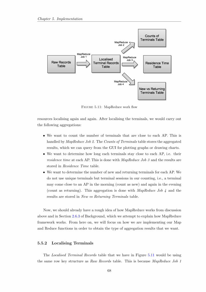
Chapter 5. Implementation
Figure 5.11: MapReduce work flow
resources localising again and again. After localising the terminals, we would carry out
the following aggregations:
• We want to count the number of terminals that are close to each AP. This is
handled by MapReduce Job 2. The Counts of Terminals table stores the aggregated
results, which we can query from the GUI for plotting graphs or drawing charts.
• We want to determine how long each terminals stay close to each AP, i.e. their
residence time at each AP. This is done with MapReduce Job 3 and the results are
stored in Residence Time table.
• We want to determine the number of new and returning terminals for each AP. We
do not use unique terminals but terminal sessions in our counting, i.e., a terminal
may come close to an AP in the morning (count as new) and again in the evening
(count as returning). This aggregation is done with MapReduce Job 4 and the
results are stored in New vs Returning Terminals table.
Now, we should already have a rough idea of how MapReduce works from discussion
above and in Section 2.6.3 of Background, which we attempt to explain how MapReduce
framework works. From here on, we will focus on how we are implementing our Map
and Reduce functions in order to obtain the type of aggregation results that we want.
5.5.2 Localising Terminals
The Localised Terminal Records table that we have in Figure 5.11 would be using
the same row key structure as Raw Records table. This is because MapReduce Job 1
68

Chapter 5. Implementation
just attempts to localise each terminal by associating it to its nearest AP by using RSSI
information, thus, it seems like we are just removing some of the extra detection records
from the Raw Records table. We will use the HBase scan feature to select the range of
rows that we want to pass into the Map function as input.
row key ap mac terminal mac rssi timestamp︸ ︷︷ ︸ ︸ ︷︷ ︸row key columns
Table 5.3: A Row Representing a Detection Record in Raw Records table and LocalisedTerminal Records table. Both tables have the same structure. The row key has the
structure that we explained earlier under Data Schema Design section.
Map function
Input key: 〈row key〉Input value: 〈ap mac, terminal mac, rssi, timestamp〉Output key: 〈terminal mac〉 − 〈time(yyyyMMddHHmmss)〉Output value: 〈row key〉 − 〈ap mac, terminal mac, rssi, timestamp〉
The input key shown above is the row key of a record as illustrated in Table 5.3
and the input value is a collection of columns within the row. Each row, representing a
detection record, that falls within the range of time we have selected using the HBase
scan, would be passed into the Map function one at a time. The Map function would
be executed once for each input key and value.
Within the Map function, we will use the timestamp that is passed in as input value
and convert it to another format that is usable such as yyyyMMddHHmmss (yearMon-
thDayHourMinuteSecond) (1). During the conversion, since we are using Unix time
format, Java would take care of any daylight saving or timezone issue for us by using
the timezone of the server this MapReduce job is execute on. With the format mention
in (1), we will round off the time to the previous 0 seconds or 30 seconds. For instance,
a terminal that is detected at a time of 2013-05-25-14-56-33 would be rounded to 2013-
05-25-14-56-30 and at a time of 2013-05-25-14-56-22 to 2013-05-25-14-56-00. We would
then emit out the output key as a concatenation of terminal mac and time using the
format in (1). What we are trying to achieve here is to classify together the records for
the same terminal, which is generated within the same 30 seconds of time. Then, we
simply pass the input value as the output value.
By emitting the records this way, those records representing the same terminal de-
tected by multiple APs within the same time interval of 30 seconds would be grouped
together under the same key 〈terminal mac and time〉. This group would then be passed
as an input to the Reduce function.
69

Chapter 5. Implementation
Reduce function
Input key: 〈terminal mac〉 − 〈time(yyyyMMddHHmmss)〉Input value: [{〈row key〉 − 〈ap mac, terminal mac, rssi, timestamp〉}] (2)
Output key: 〈row key〉Output value: 〈ap mac, terminal mac, rssi, timestamp〉
The output of the Map phase would becomes the input of the Reduce phase. After
the Map phase, those output values sharing the same key would be grouped together.
The input value of the Reduce function is a list of records sharing the same key. We
would iterate over this list and find out the record with the highest RSSI value. We
would then output the row key of that record, which can be obtained from (2), and the
columns for that record also from (2).
Minimise “Ping Pong” effect
After conducting an experiment, which we will cover in Chapter 6 (Evaluation), we
notice that there is a “Ping Pong” effect happening. “Ping Pong” effect happens when
the received signal strength becomes unreliable at times leading to a WiFi terminal
being associated with one AP at one time and to another at subsequent time although
the terminal has not moved. This effect is most commonly observed when a terminal is
located directly in between two APs.
In order to fix this problem, we sort the list of records from the input value of the
Reduce function using natural ordering on the ap mac from each record. We would
then introduce a RSSI DIFF THRESHOLD when comparing the RSSI value between
two records. If one record has RSSI value higher than another record by 5, we will choose
the former one. But if a record has RSSI value higher only by 3 than another one, we
will not consider choosing the former. The natural ordering introduce a precedence or
favour for a record detected by a particular AP. The RSSI DIFF THRESHOLD serves
to break this precedence or favour for a record with RSSI that is distinctively higher.
This would slightly reduce the effect of “Ping Pong”, in which we end up localising a
terminal to one AP at one time and to another at subsequent time, just because there
is a small improvement in RSSI value for the latter.
Object reference error
During the time we worked on this localisation algorithm, there was one particular
bug, which caused us to spend a lot of time in trying to debug. This is because we do
not know whether the error happens in the way HBase execute our Map and Reduce
functions or there is error in our code. From Listing 5.6, we can see that everything seems
70

Chapter 5. Implementation
12 //Put is an object representing a row in an Hbase table3 Put closestRecord = null;4 int bestRssi = −300;56 for (Put p : values) {7 int rssi = ... //Get RSSI encapsulated in p89 int rssiDiff = rssi − bestRssi;
10 if(rssiDiff > RSSI DIFF THRESHOLD){11 bestRssi = rssi;12 closestRecord = p;13 }14 }15 ...
Listing 5.6: Illustrating a bug in object reference.
to look fine. However, on Line 12, when we store the reference of p, a row (representing
a record) with the highest RSSI so far, to closestRecord, this reference is not persistent.
What we discover is although we reference to the p in the current iteration, Java still
discard that p object for that iteration. The final result of closestRecord actually always
reference the p from the last iteration of the for loop. In order to solve this problem,
we realise that HBase client package provides a method for cloning a Put object by
constructing a new object with the same state as the existing one. In Listing 5.7, we
replace Line 12 in the previous listing with the new code to fix the problem.
1 Put tempPut = new Put(p);2 closestRecord = tempPut;3 ...
Listing 5.7: Illustrating a bug in object reference.
5.5.3 Count Statistics
After localising the terminals by associating them to their closest AP, we would
have the aggregated results in Localised Terminal Records table. From here on, all our
aggregations, namely counting, residence time and new versus returning, would make
use of data from Localised Terminal Records table. For this section on Count Statistics,
our objective is to count the number of terminals that are close to each AP. After
this aggregation, we would store the results in Counts of Terminals table, which we
have mentioned in Figure 5.11. It should be noted that we are counting the number of
terminals that are close to each AP during a 1 minute interval.
71

Chapter 5. Implementation
Map function
Input key: 〈row key〉Input value: 〈ap mac, terminal mac, rssi, timestamp〉
〈ap mac〉 − 〈time(yyyyMMddHHmm)〉 〈terminal mac〉︸ ︷︷ ︸ ︸ ︷︷ ︸Map output key Map output value
Table 5.4: Count Statistics Map Function Output Key and Value
The input key shown above is the row key of a row (representing a record) in Localised
Terminal Records table and the input value is a collection of columns within the row.
Table 5.4 shows the output key and value of the Map function.
Within the Map function, we will use the timestamp that is passed in as input value
and convert it to another format that is usable such as yyyyMMddHHmm (yearMon-
thDayHourMinute) (3). We position the year portion to the far left of the format in
(3) since it has higher precedence. Notice that this time round, we chop off the sec-
ond part of the time format when compared to previous section on Localising Terminal.
This is because we want to count only those records for different terminals11 that are
generated within the current minute. For example, a terminal is detected at 2013-05-25-
14-56-22 (at 2:56:22PM) and another terminal is detected at 2013-05-25-14-56-51 (at
2:56:51PM), we would consider counting both terminals for the time interval 2013-05-
25-14-56 (at 2:56PM) by chopping off the seconds part of the time. Hence, we will emit
out an output key from the Map function as 〈ap mac〉 − 〈time(yyyyMMddHHmm)〉,e.g. 〈AA : BB : CC : DD : EE : FF 〉 − 〈201305251456〉, since we want all records
detected by the same AP within the same time interval to be grouped together. The
output value is the terminal mac. We choose to emit out this value for a reason that we
will explain under the Reduce function below.
Reduce function
Input key: 〈ap mac〉 − 〈time(yyyyMMddHHmm)〉Input value: [{terminal mac}] (4)
Output key: 〈ap mac〉 − 〈time(yyyyMMdd)〉Output value: 〈no counts〉
Within the Reduce function, we would be receiving all the MAC addresses of termi-
nals that are being detected by an AP specified by the ap mac input key. This means
11Note that we have already done the localising of terminals and we are using the aggregated resultsin Localising Terminal table.
72

Chapter 5. Implementation
that after the Map phase, all the terminals that are being detected by the same AP
would be grouped together under the same key and this would be passed to the Reduce
function as a group of terminals’ MAC addresses. In (4), we receive as input value a list
of MAC addresses.
Since we are scanning every 30 seconds and within a 1 minute interval, 2 detection
records for the same terminal are pushed to the server, there is a possibility that we detect
a terminal at say 12:50:13PM and again at 12:50:45PM. The time is not 12:50:43PM
(after 30 seconds elapsed) because we consider that there could be a few seconds of
transmission delay12 and in this example, we just take that as 2 seconds. We would
not want to count the terminal twice, which contributes to the double counting problem.
Hence, we use a HashMap and add each terminal MAC address to the map data structure,
using MAC address as the key of the map and simply use integer value of 1 as value.
Note that HashMap does not allow duplicate keys, which is what we want.
Then, we can obtain the total counts of terminals close to an AP by getting the size
of the HashMap as that would indicate how many key-value elements are there in the
map. This would tell us the number of unique terminals we have detected within the 1
minute interval.
Improvement to how we store the results
Figure 5.12: Structure of Counts of Terminals table
In Figure 5.12, we have illustrated how we are storing the results from the Reduce
function in Counts of Terminals table. The row key is a composition of ap mac and
date. details is the column family and the column qualifier indicates the time interval
(HHmm) corresponding to the number of counts for that interval, e.g. there are 2 counts
for the interval 1249 which represents the period from 12:49:00PM to 12:59:00PM for
the example in Figure 5.12.
Initially, we do not store the data like the one shown in the figure. We make use of
a different row key design using 〈ap mac〉 − 〈time(yyyyMMddHHmm)〉. We include
the HHmm in the row key instead but this means the we will end up having many rows,
which is not that practical in the long term and also hard for us to query the results
from the front-end GUI.
12Remember that we are adding timestamp at Processing Agent.
73

Chapter 5. Implementation
5.5.4 Residence Time
In order to find out how long each WiFi terminal, indirectly the user, stays close to
an AP, we need to write a much more sophisticated algorithm in the Reduce function
than the one we have before. We would be analysing the traces of a terminal for the
whole day across all our deployed APs.
Since we have the records of a terminal being detected by any of our APs across
the day in the Localised Terminal Records table, we could project out the traces of a
terminal within the day by sorting the detection records according to the timestamp of
each record as illustrated in Figure 5.13. If we have more time for this project, from
these traces, we could even attempt to analyse how a user move within the environment
we are monitoring. This could be combined with the Residence Time MapReduce job.
Map function
terminal mac ap mac, terminal mac, rssi, timestamp︸ ︷︷ ︸ ︸ ︷︷ ︸Map output key Map output value
Table 5.5: Residence Time Map Function Output Key and Value
Each row (representing a record) from the Localised Terminal Records table would
be an input to the Map function. In other words, the Map function would be applied to
each row in Localised Terminal Records one by one. In the Map function, we will emit
out the terminal mac as the output key and the whole record (ap mac, terminal mac,
rssi, timestamp) as output value as illustrated in Table 5.5.
Reduce function
After the Map phase, since we have emitted out terminal mac as the Map output key,
all the detection records belonging to a terminal would be grouped together under the
same key, terminal mac in this case. Hence, we will receive terminal mac as an input
key in the Reduce function and a list of records ([{ap mac, terminal mac, rssi and
timestamp}]) as input value. We will iterate over this list of records and attempt to
sort these records according to the timestamp, by ascending order of time. Figure 5.13
shows an example illustrating part of the traces of a terminal’s presence across the day,
sorted by the timestamp and show information such as which AP detects the terminal
and what is the RSSI associated.
74
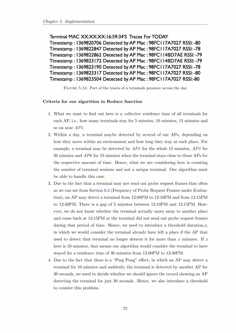
Chapter 5. Implementation
Figure 5.13: Part of the traces of a terminals presence across the day
Criteria for our algorithm in Reduce function
1. What we want to find out here is a collective residence time of all terminals for
each AP, i.e., how many terminals stay for 5 minutes, 10 minutes, 15 minutes and
so on near AP1.
2. Within a day, a terminal maybe detected by several of our APs, depending on
how they move within an environment and how long they stay at each place. For
example, a terminal may be detected by AP1 for the whole 15 minutes, AP3 for
30 minutes and AP6 for 10 minutes when the terminal stays close to these APs for
the respective amount of time. Hence, what we are considering here is counting
the number of terminal sessions and not a unique terminal. Our algorithm must
be able to handle this case.
3. Due to the fact that a terminal may not send out probe request frames that often
as we can see from Section 6.3 (Frequency of Probe Request Frames under Evalua-
tion), an AP may detect a terminal from 12:00PM to 12:10PM and from 12:15PM
to 12:30PM. There is a gap of 5 minutes between 12:10PM and 12:15PM. How-
ever, we do not know whether the terminal actually move away to another place
and come back at 12:15PM or the terminal did not send out probe request frames
during that period of time. Hence, we need to introduce a threshold duration,x,
in which we would consider the terminal already have left a place if the AP that
used to detect that terminal no longer detects it for more than x minutes. If x
here is 10 minutes, that means our algorithm would consider the terminal to have
stayed for a residence time of 30 minutes from 12:00PM to 12:30PM.
4. Due to the fact that there is a “Ping Pong” effect, in which an AP may detect a
terminal for 10 minutes and suddenly, the terminal is detected by another AP for
30 seconds, we need to decide whether we should ignore the record showing an AP
detecting the terminal for just 30 seconds. Hence, we also introduce a threshold
to counter this problem.
75
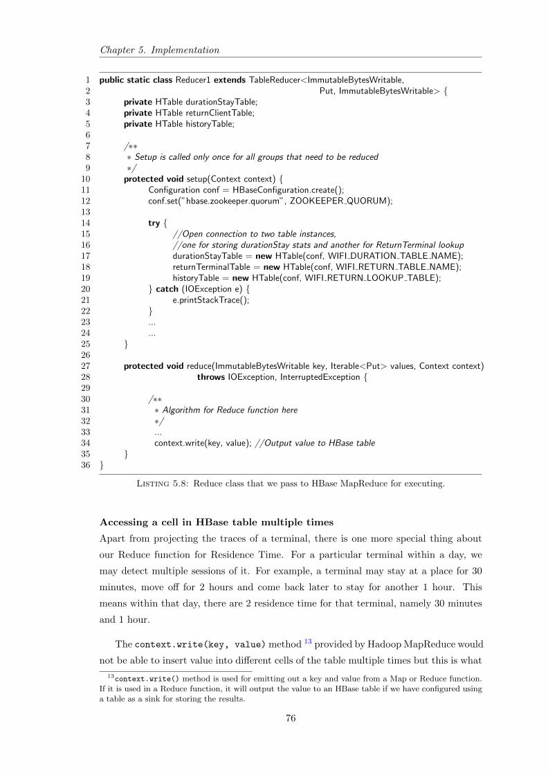
Chapter 5. Implementation
1 public static class Reducer1 extends TableReducer<ImmutableBytesWritable,2 Put, ImmutableBytesWritable> {3 private HTable durationStayTable;4 private HTable returnClientTable;5 private HTable historyTable;67 /∗∗8 ∗ Setup is called only once for all groups that need to be reduced9 ∗/
10 protected void setup(Context context) {11 Configuration conf = HBaseConfiguration.create();12 conf.set(”hbase.zookeeper.quorum”, ZOOKEEPER QUORUM);1314 try {15 //Open connection to two table instances,16 //one for storing durationStay stats and another for ReturnTerminal lookup17 durationStayTable = new HTable(conf, WIFI DURATION TABLE NAME);18 returnTerminalTable = new HTable(conf, WIFI RETURN TABLE NAME);19 historyTable = new HTable(conf, WIFI RETURN LOOKUP TABLE);20 } catch (IOException e) {21 e.printStackTrace();22 }23 ...24 ...25 }2627 protected void reduce(ImmutableBytesWritable key, Iterable<Put> values, Context context)28 throws IOException, InterruptedException {2930 /∗∗31 ∗ Algorithm for Reduce function here32 ∗/33 ...34 context.write(key, value); //Output value to HBase table35 }36 }
Listing 5.8: Reduce class that we pass to HBase MapReduce for executing.
Accessing a cell in HBase table multiple times
Apart from projecting the traces of a terminal, there is one more special thing about
our Reduce function for Residence Time. For a particular terminal within a day, we
may detect multiple sessions of it. For example, a terminal may stay at a place for 30
minutes, move off for 2 hours and come back later to stay for another 1 hour. This
means within that day, there are 2 residence time for that terminal, namely 30 minutes
and 1 hour.
The context.write(key, value) method 13 provided by Hadoop MapReduce would
not be able to insert value into different cells of the table multiple times but this is what
13context.write() method is used for emitting out a key and value from a Map or Reduce function.If it is used in a Reduce function, it will output the value to an HBase table if we have configured usinga table as a sink for storing the results.
76
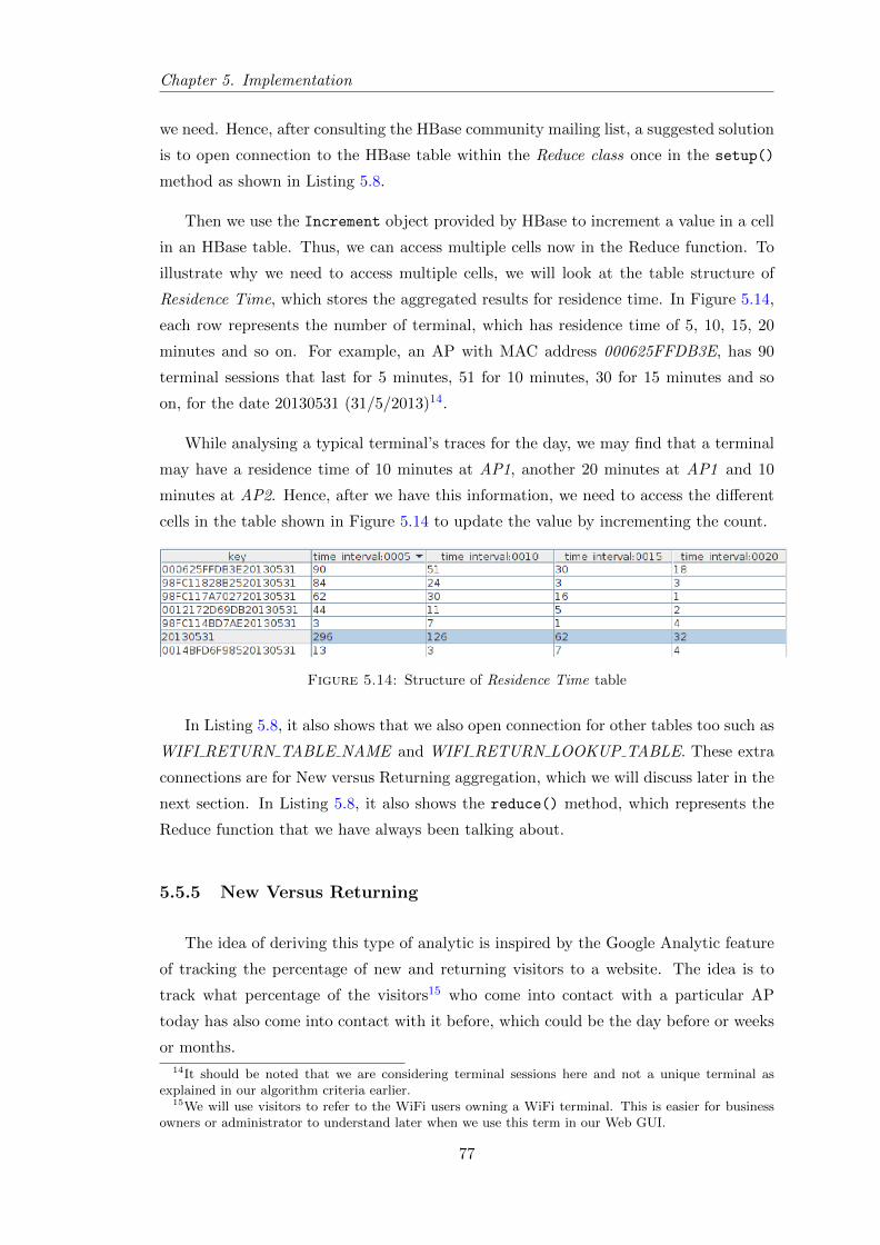
Chapter 5. Implementation
we need. Hence, after consulting the HBase community mailing list, a suggested solution
is to open connection to the HBase table within the Reduce class once in the setup()
method as shown in Listing 5.8.
Then we use the Increment object provided by HBase to increment a value in a cell
in an HBase table. Thus, we can access multiple cells now in the Reduce function. To
illustrate why we need to access multiple cells, we will look at the table structure of
Residence Time, which stores the aggregated results for residence time. In Figure 5.14,
each row represents the number of terminal, which has residence time of 5, 10, 15, 20
minutes and so on. For example, an AP with MAC address 000625FFDB3E, has 90
terminal sessions that last for 5 minutes, 51 for 10 minutes, 30 for 15 minutes and so
on, for the date 20130531 (31/5/2013)14.
While analysing a typical terminal’s traces for the day, we may find that a terminal
may have a residence time of 10 minutes at AP1, another 20 minutes at AP1 and 10
minutes at AP2. Hence, after we have this information, we need to access the different
cells in the table shown in Figure 5.14 to update the value by incrementing the count.
Figure 5.14: Structure of Residence Time table
In Listing 5.8, it also shows that we also open connection for other tables too such as
WIFI RETURN TABLE NAME and WIFI RETURN LOOKUP TABLE. These extra
connections are for New versus Returning aggregation, which we will discuss later in the
next section. In Listing 5.8, it also shows the reduce() method, which represents the
Reduce function that we have always been talking about.
5.5.5 New Versus Returning
The idea of deriving this type of analytic is inspired by the Google Analytic feature
of tracking the percentage of new and returning visitors to a website. The idea is to
track what percentage of the visitors15 who come into contact with a particular AP
today has also come into contact with it before, which could be the day before or weeks
or months.
14It should be noted that we are considering terminal sessions here and not a unique terminal asexplained in our algorithm criteria earlier.
15We will use visitors to refer to the WiFi users owning a WiFi terminal. This is easier for businessowners or administrator to understand later when we use this term in our Web GUI.
77
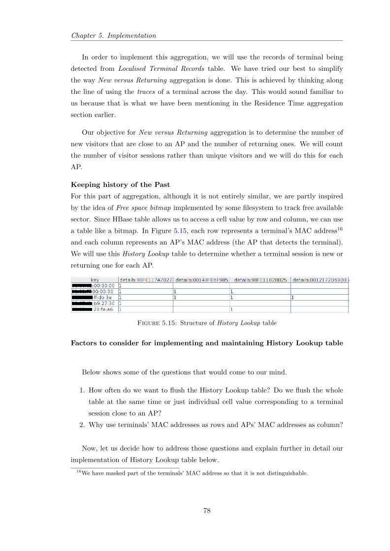
Chapter 5. Implementation
In order to implement this aggregation, we will use the records of terminal being
detected from Localised Terminal Records table. We have tried our best to simplify
the way New versus Returning aggregation is done. This is achieved by thinking along
the line of using the traces of a terminal across the day. This would sound familiar to
us because that is what we have been mentioning in the Residence Time aggregation
section earlier.
Our objective for New versus Returning aggregation is to determine the number of
new visitors that are close to an AP and the number of returning ones. We will count
the number of visitor sessions rather than unique visitors and we will do this for each
AP.
Keeping history of the Past
For this part of aggregation, although it is not entirely similar, we are partly inspired
by the idea of Free space bitmap implemented by some filesystem to track free available
sector. Since HBase table allows us to access a cell value by row and column, we can use
a table like a bitmap. In Figure 5.15, each row represents a terminal’s MAC address16
and each column represents an AP’s MAC address (the AP that detects the terminal).
We will use this History Lookup table to determine whether a terminal session is new or
returning one for each AP.
Figure 5.15: Structure of History Lookup table
Factors to consider for implementing and maintaining History Lookup table
Below shows some of the questions that would come to our mind.
1. How often do we want to flush the History Lookup table? Do we flush the whole
table at the same time or just individual cell value corresponding to a terminal
session close to an AP?
2. Why use terminals’ MAC addresses as rows and APs’ MAC addresses as column?
Now, let us decide how to address those questions and explain further in detail our
implementation of History Lookup table below.
16We have masked part of the terminals’ MAC address so that it is not distinguishable.
78
Chapter 5. Implementation
1. Fortunately and coincidentally, HBase provides a feature called Time-To-Live
(TTL) that we can set at a column family level. This means that if we spec-
ify 18,000 seconds as TTL value for a column family x, any cells that are under
x will expire after 18,000 seconds has elapsed starting from the time each cell is
created. Hence, we can flush history on a cell by cell basis, which is really beautiful
by setting the TTL.
2. We store a terminal’s MAC address as the row key and AP’s MAC address as the
column qualifier because HBase has the capability to allow us to have billions of
rows and millions of columns. Since we may detect massive number of MAC ad-
dresses from terminals that come across any of our APs (assuming for commercial
deployment) and only not more than a few thousands of APs, we can safely store
the data this way.
3. History is stored per AP and not system wide. A visitor that have been to AP1
but not AP2 would be a returning visitor for AP1 but treated as a new visitor to
AP2.
4. HBase stores free null values. If a cell has no value, there is no allocation of space
for the cell in HBase. In contrast, relational SQL explicitly stores the null value or
allocate a space for it. This feature of HBase makes using a History Lookup table
like what we have done an ideal choice.
5.5.6 Summary
We have been discussing a lot about aggregation and it is really a painful and
headache process to go through the raw data when something goes wrong. This is
one of the most challenging part of this project too since we have no experience before
in data analytic of such scale.
As we can see from all types of aggregations so far, the design of the row key for Raw
Records table and Localised Terminal Records table is very important since we make use
of them extensively during the MapReduce process in each types of aggregation we have
discussed above.
MapReduce concept might be easy to understand but the algorithms involved in
each of the functions might require some time to digest. Hence, we hope that we have
at least given the gist of how we are aggregating the data without going too much into
the deep detail of the actual implementation.
79
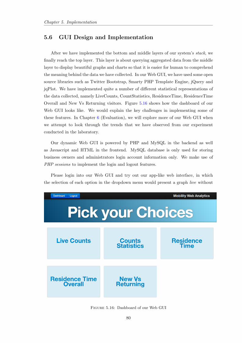
Chapter 5. Implementation
5.6 GUI Design and Implementation
After we have implemented the bottom and middle layers of our system’s stack, we
finally reach the top layer. This layer is about querying aggregated data from the middle
layer to display beautiful graphs and charts so that it is easier for human to comprehend
the meaning behind the data we have collected. In our Web GUI, we have used some open
source libraries such as Twitter Bootstrap, Smarty PHP Template Engine, jQuery and
jqPlot. We have implemented quite a number of different statistical representations of
the data collected, namely LiveCounts, CountStatistics, ResidenceTime, ResidenceTime
Overall and New Vs Returning visitors. Figure 5.16 shows how the dashboard of our
Web GUI looks like. We would explain the key challenges in implementing some of
these features. In Chapter 6 (Evaluation), we will explore more of our Web GUI when
we attempt to look through the trends that we have observed from our experiment
conducted in the laboratory.
Our dynamic Web GUI is powered by PHP and MySQL in the backend as well
as Javascript and HTML in the frontend. MySQL database is only used for storing
business owners and administrators login account information only. We make use of
PHP sessions to implement the login and logout features.
Please login into our Web GUI and try out our app-like web interface, in which
the selection of each option in the dropdown menu would present a graph live without
Figure 5.16: Dashboard of our Web GUI
80
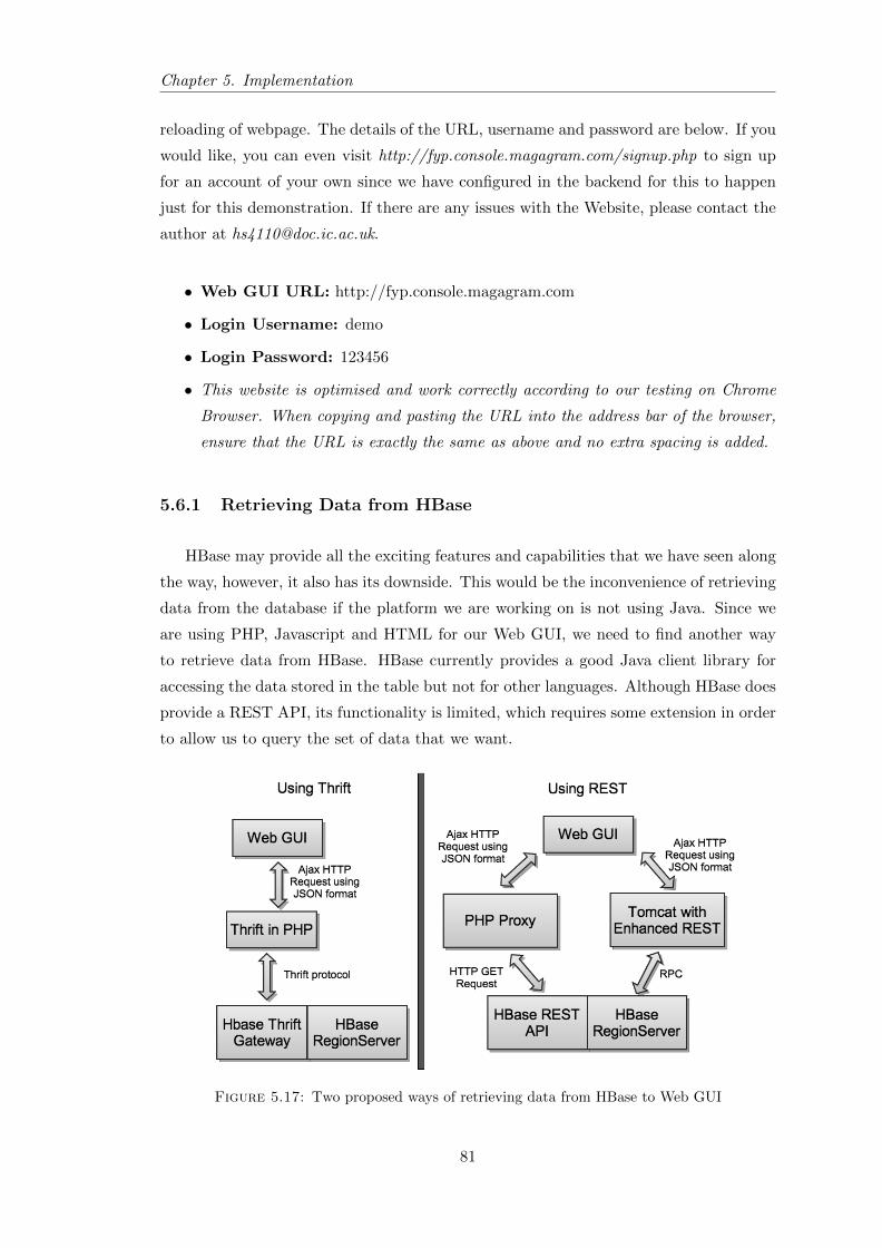
Chapter 5. Implementation
reloading of webpage. The details of the URL, username and password are below. If you
would like, you can even visit http://fyp.console.magagram.com/signup.php to sign up
for an account of your own since we have configured in the backend for this to happen
just for this demonstration. If there are any issues with the Website, please contact the
author at [email protected].
• Web GUI URL: http://fyp.console.magagram.com
• Login Username: demo
• Login Password: 123456
• This website is optimised and work correctly according to our testing on Chrome
Browser. When copying and pasting the URL into the address bar of the browser,
ensure that the URL is exactly the same as above and no extra spacing is added.
5.6.1 Retrieving Data from HBase
HBase may provide all the exciting features and capabilities that we have seen along
the way, however, it also has its downside. This would be the inconvenience of retrieving
data from the database if the platform we are working on is not using Java. Since we
are using PHP, Javascript and HTML for our Web GUI, we need to find another way
to retrieve data from HBase. HBase currently provides a good Java client library for
accessing the data stored in the table but not for other languages. Although HBase does
provide a REST API, its functionality is limited, which requires some extension in order
to allow us to query the set of data that we want.
Figure 5.17: Two proposed ways of retrieving data from HBase to Web GUI
81

Chapter 5. Implementation
In Figure 5.17, we have proposed two ways of retrieving data from HBase.
1. Using Thrift: Thrift is a RPC software framework for scalable cross-language
communication [30]. Thrift has support for many programming languages but it
requires us to define an Interface Definition Language (IDL) to create a Thrift
service in a language we are working on. In our case, the language is PHP. HBase
has a Thrift Gateway module that can be installed on the same server as Region-
Server (server that stores small chunks of the table). However, we are required
to use the Thrift IDL file for HBase to generate a Thrift service for PHP. The
current documentation for doing this is not very clear and after spending some
time studying the feasibility of using Thrift, we think that it would not worth the
effort since we do not have enough support for this method.
2. Using REST: HBase provides a REST17 API that allows us to query for data in
some way. We can query for a whole row from an HBase table by specifying the
row key in a URI, e.g. http://hbase-rest/table name/row key. However, although
on HBase wiki, there is a scan feature which we can specify a range of rows we
want to query, the feature does not seem to work after much effort. Hence, we
decide to implement this scan feature in Java by utilising the HBase Java client
package and deploy this module on Tomcat. We call our module HBaseEnhance-
dREST, which is shown in Figure 5.17 as Tomcat with Enhanced REST.
Since we want to use Javascript extensively to create an app-like effect for
our Web GUI, we need to make jQuery Ajax HTTP GET request18 directly in
Javascript. However, there is a cross-domain restriction policy imposed by all
browsers for security reason, which state that any direct Ajax HTTP GET request
to a server requires that the server respond with Content Header set to includes
“Access-Control-Allow-Origin: *”. This means that the server allow access from
any origin, hence, the browser would trust that the server permits it to make Ajax
HTTP GET request to it. If no such Content Header is set, the browser will not
accept the server’s response.
HBase REST API does not set Content Header to include “Access-Control-
Allow-Origin: *”, hence, we cannot directly make Ajax GET request to HBase
REST API in Javascript. The only work around is by setting up a PHP Proxy as
17REST is a software architecture that involves client-server, in which the server provides a standard-ised application programming interface for accessing and modifying data.
18jQuery Ajax HTTP GET request is a method provided by jQuery Javascript library to get datafrom a server on a client-side using HTTP.
82

Chapter 5. Implementation
shown in Figure 5.17. We use the open source Simple PHP Proxy [15]. This proxy
basically just accepts Ajax HTTP GET request from the Web GUI in Javascript
and forward that using PHP cURL module to the HBase REST API. Since PHP
cURL does not requires the server’s response Content Header to include “Access-
Control-Allow-Origin: *”, it can interact with HBase REST API without any
problems. When the data returns from HBase, the proxy would pass it to the Web
GUI with proper Content Header set. It should be noted that the Thrift in PHP
shown in Figure 5.17 would have to do the same thing of setting proper Content
Header.
After some analysis and experimentations, we decide to use the second approach
above, Using REST. This is because the Thrift approach does not promise a working
solution while we know the REST approach is much more feasible in terms of implemen-
tation. Thus, if we want to retrieve a whole row or any rows from HBase, we will use
the default HBase REST API via our PHP Proxy. If we want to use the scan feature to
query a range of rows from HBase, we will use our HBaseEnhancedREST API, which
we have implemented.
Javascript Bytes Utility and REST wrapper
HBase REST has another problem, which we need to overcome. However, this is a
common problem for everyone and if we manage to solve it, it would bring great benefits
to the whole HBase community. Currently, if anyone wants to use the HBase REST,
the data type for each cell in the table can only be string, which opposes the original
idea of HBase being flexible on data types and schema.
Let us explain why this is happening. HBase stores the value of the cell in bytes
and this value could be of any data types. If the developers can retrieve these bytes
from HBase table, they would have known how to decode it since they know what data
types these bytes represent. Since HBase REST uses JSON format to transmit the
queried data to a client-side, it is not possible to represent bytes in JSON. Hence, the
bytes have to be encoded somehow before it is transmitted to the client-side. However,
HBase REST is just like a middle man who does not know what the bytes for these
cell represent, hence, it could not autonomously interpret the data types of these cell
values and convert them to their corresponding data types. Therefore, HBase basically
states that if we want to use HBase REST, we must store the content of each cell in
the table in string so that HBase REST knows that the bytes represent string. HBase
REST converts the cell value in bytes to string first and then use Base64 19 to encode
19Base64 is a scheme used to represent binary data in ASCII string standard.
83
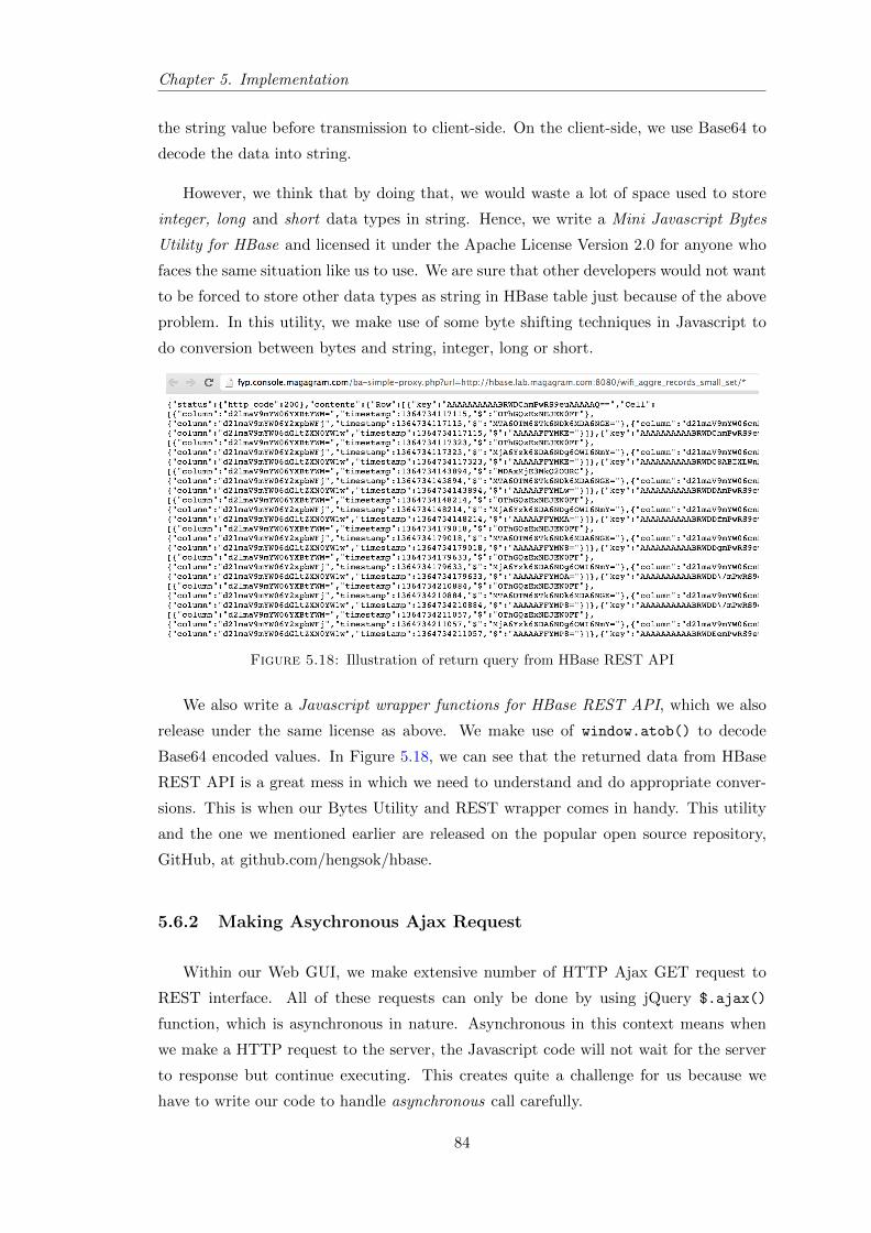
Chapter 5. Implementation
the string value before transmission to client-side. On the client-side, we use Base64 to
decode the data into string.
However, we think that by doing that, we would waste a lot of space used to store
integer, long and short data types in string. Hence, we write a Mini Javascript Bytes
Utility for HBase and licensed it under the Apache License Version 2.0 for anyone who
faces the same situation like us to use. We are sure that other developers would not want
to be forced to store other data types as string in HBase table just because of the above
problem. In this utility, we make use of some byte shifting techniques in Javascript to
do conversion between bytes and string, integer, long or short.
Figure 5.18: Illustration of return query from HBase REST API
We also write a Javascript wrapper functions for HBase REST API, which we also
release under the same license as above. We make use of window.atob() to decode
Base64 encoded values. In Figure 5.18, we can see that the returned data from HBase
REST API is a great mess in which we need to understand and do appropriate conver-
sions. This is when our Bytes Utility and REST wrapper comes in handy. This utility
and the one we mentioned earlier are released on the popular open source repository,
GitHub, at github.com/hengsok/hbase.
5.6.2 Making Asychronous Ajax Request
Within our Web GUI, we make extensive number of HTTP Ajax GET request to
REST interface. All of these requests can only be done by using jQuery $.ajax()
function, which is asynchronous in nature. Asynchronous in this context means when
we make a HTTP request to the server, the Javascript code will not wait for the server
to response but continue executing. This creates quite a challenge for us because we
have to write our code to handle asynchronous call carefully.
84

Chapter 5. Implementation
For instance, after a user chooses a date amongst the options of a dropdown menu,
we make an asynchronous HTTP GET request to the server to fetch the data for that
date. However, how would we know when the data comes back from the server so that
we could start plotting the graphs. This is done using a beautiful feature in Javascript
called promise. Promise is a programming construct that have been introduced since
1976 [33].
12 var promise = REST.getAllRowsAllCols(restEndpoint,”TABLE NAME”);34 promise.success(function (data) {5 if(data.status.http code == 200){6 //use data safely here7 }8 });
Listing 5.9: Using Javascript promise to manage asynchronous function call.
In Listing 5.9, REST.getAllRowsAllCols() is an asynchronous function call. We
make this call and store the promise that it returns. In REST.getAllRowsAllCols()
function, we return a promise. Then we have the handler promise.success(), which
will be invoked when the asynchronous call succeeds. We could then call any other
functions or do something within this handler.
5.6.3 CountLive and CountStatistics
Figure 5.19: Illustration of CountLive page in Web GUI
85
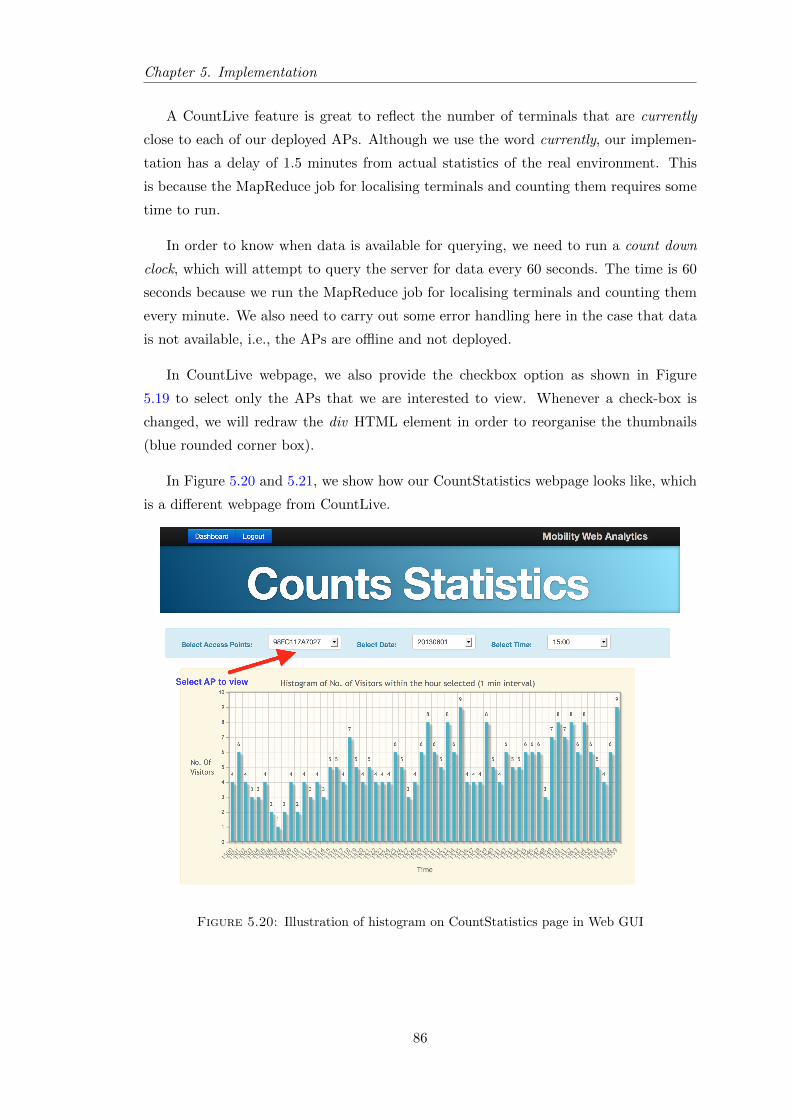
Chapter 5. Implementation
A CountLive feature is great to reflect the number of terminals that are currently
close to each of our deployed APs. Although we use the word currently, our implemen-
tation has a delay of 1.5 minutes from actual statistics of the real environment. This
is because the MapReduce job for localising terminals and counting them requires some
time to run.
In order to know when data is available for querying, we need to run a count down
clock, which will attempt to query the server for data every 60 seconds. The time is 60
seconds because we run the MapReduce job for localising terminals and counting them
every minute. We also need to carry out some error handling here in the case that data
is not available, i.e., the APs are offline and not deployed.
In CountLive webpage, we also provide the checkbox option as shown in Figure
5.19 to select only the APs that we are interested to view. Whenever a check-box is
changed, we will redraw the div HTML element in order to reorganise the thumbnails
(blue rounded corner box).
In Figure 5.20 and 5.21, we show how our CountStatistics webpage looks like, which
is a different webpage from CountLive.
Figure 5.20: Illustration of histogram on CountStatistics page in Web GUI
86
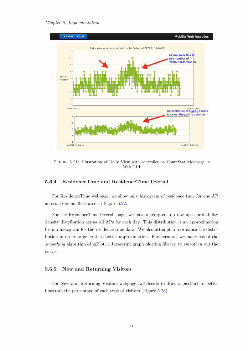
Chapter 5. Implementation
Figure 5.21: Illustration of Daily View with controller on CountStatistics page inWeb GUI
5.6.4 ResidenceTime and ResidenceTime Overall
For ResidenceTime webpage, we show only histogram of residence time for one AP
across a day as illustrated in Figure 5.22.
For the ResidenceTime Overall page, we have attempted to draw up a probability
density distribution across all APs for each day. This distribution is an approximation
from a histogram for the residence time data. We also attempt to normalise the distri-
bution in order to generate a better approximation. Furthermore, we make use of the
smoothing algorithm of jqPlot, a Javascript graph plotting library, to smoothen out the
curve.
5.6.5 New and Returning Visitors
For New and Returning Visitors webpage, we decide to draw a piechart to better
illustrate the percentage of each type of visitors (Figure 5.23).
87
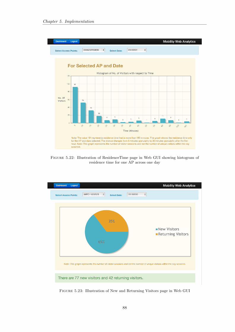
Chapter 5. Implementation
Figure 5.22: Illustration of ResidenceTime page in Web GUI showing histogram ofresidence time for one AP across one day
Figure 5.23: Illustration of New and Returning Visitors page in Web GUI
88

Chapter 6
Evaluation
6.1 Setting up of Experiment in Laboratory
After implementing a system to track WiFi terminals, we should put it to a good
test. There is a couple of issues that almost prevent us from conducting an experiment
in the Department Of Computing laboratory successfully.
Firstly, our university’s network and security team was concerned that our APs might
interrupt the experience of using wireless internet access by individual students in the
laboratory. These include radio signal interference and some students may unexpectedly
connect to our APs. To solve part of these problems, we disable the broadcast of SSID
across all our APs. Even if a terminal knows our SSID, we use WEP as a simple
protection to prevent it from connecting to our APs.
Secondly, our department was concerned that it would be hard to wire our APs to
the department’s existing network. In order to solve this problem, we had decided to
setup our own private network by linking up all our APs wirelessly by setting some APs
into client bridge mode and some into repeater bridge mode. We used another AP, which
really worked in AP infrastructure mode but not connected to the university’s network,
as the main AP that other APs would connect to and extend the network. This allows
us to have a wireless private network in which each of the APs can communicate with
each other easily. Our main objective is to allow each AP to have access to a central
Processing Agent so that it could sent the collected data to it.
Finally, since our university’s network and security team was concerned that our
APs may exist in AP infrastructure mode, our APs are not allowed to connect to the
school’s network to gain internet access. Hence, we could not send the data collected to
the database, which is hosted somewhere else on the internet. To solve this problem, we
attempted to buy a 3G Dongle from O2 in order to provide internet access via one of
our APs. This could be done since we have a Mini 3G AP from TP-Link, which allows
us to connect the 3G Dongle to it and there is a RJ-45 port on the Mini 3G AP that
provides internet access via Ethernet. Hence, we can connect one of our APs using this
port and all our other APs would be configured to receive the internet connectivity as
well.
89

Chapter 6. Evaluation
After successfully tested out this idea, we realised that everything works according
to what we expected. However, there was one issue with high latency caused by the
unstable 3G connection. Sometimes, the 3G connection would lose internet connectivity
for a short period of time before regaining. This means that if we use this method of
providing internet access to our APs, there may be period of time where there are inter-
ruptions. Even after we have implemented the error handling, which we have explained
in Implementation chapter, we believe this mode of providing internet connectivity is
too unreliable.
Therefore, we thought again of other alternatives. We came up with an alternative,
which promised to allow us to run the experiment in the laboratory successfully. We
connected a laptop to the main AP, which we have mentioned before, to provide the
laptop access to the private network that we had set up. We bought an extra USB WiFi
adapter and plugged into the laptop to provide a second network interface for the laptop.
Then, we changed the priority of the network cards/interfaces on Windows 8, which our
laptop had installed so that the laptop could still have internet access via one interface
and access to our private network via another. If we do not do this, we would not be
able to get internet access on the laptop (running Windows) when another interface is
connected to a private network.
The laptop served as a central Processing Agent in which we deployed our servlet
on it using Tomcat. All APs had network access to this agent and they would push
all collected data to it. Then, this agent would process the data, insert timestamp and
establish a connection to the database to push the processed data to the database hosted
on the internet.
Ideally, in the future, we require that all our APs would have internet connectivity,
which should be the case since they are APs.
6.1.1 Deployment Overview
In Figure 6.1, it shows an overview of our deployment in the laboratory. Since we
do not want to publish the map of our laboratory, we have shown only the locations,
which we deployed our APs. We purposely deployed AP3 and AP2 close together to see
whether our aggregation algorithm is working correctly. Indeed, we did observe a strong
“Ping Pong” effect from the data we collected between these 2 APs, which prompted
us to alter our Localising Terminal algorithm to introduce a threshold. This serves to
indicate that our Localising Terminal aggregation is working properly after the change
to our algorithm. In the figure, it also could be seen that AP2 is placed very close to
the corridor. This is because it acts as a repeater bridge in which AP1 can connects to
90
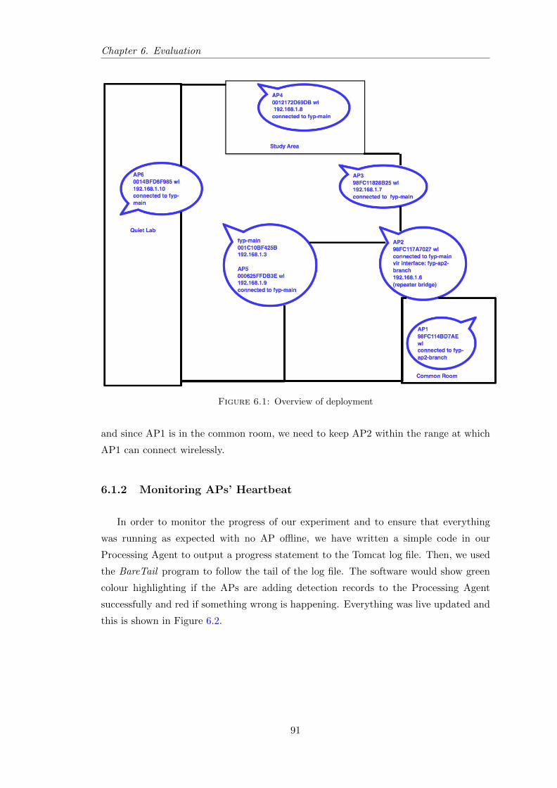
Chapter 6. Evaluation
Figure 6.1: Overview of deployment
and since AP1 is in the common room, we need to keep AP2 within the range at which
AP1 can connect wirelessly.
6.1.2 Monitoring APs’ Heartbeat
In order to monitor the progress of our experiment and to ensure that everything
was running as expected with no AP offline, we have written a simple code in our
Processing Agent to output a progress statement to the Tomcat log file. Then, we used
the BareTail program to follow the tail of the log file. The software would show green
colour highlighting if the APs are adding detection records to the Processing Agent
successfully and red if something wrong is happening. Everything was live updated and
this is shown in Figure 6.2.
91
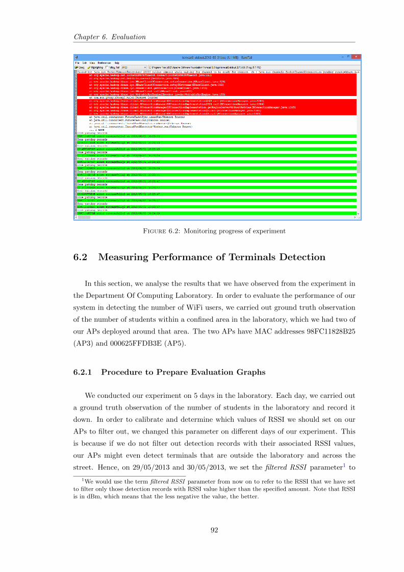
Chapter 6. Evaluation
Figure 6.2: Monitoring progress of experiment
6.2 Measuring Performance of Terminals Detection
In this section, we analyse the results that we have observed from the experiment in
the Department Of Computing Laboratory. In order to evaluate the performance of our
system in detecting the number of WiFi users, we carried out ground truth observation
of the number of students within a confined area in the laboratory, which we had two of
our APs deployed around that area. The two APs have MAC addresses 98FC11828B25
(AP3) and 000625FFDB3E (AP5).
6.2.1 Procedure to Prepare Evaluation Graphs
We conducted our experiment on 5 days in the laboratory. Each day, we carried out
a ground truth observation of the number of students in the laboratory and record it
down. In order to calibrate and determine which values of RSSI we should set on our
APs to filter out, we changed this parameter on different days of our experiment. This
is because if we do not filter out detection records with their associated RSSI values,
our APs might even detect terminals that are outside the laboratory and across the
street. Hence, on 29/05/2013 and 30/05/2013, we set the filtered RSSI parameter1 to
1We would use the term filtered RSSI parameter from now on to refer to the RSSI that we have setto filter only those detection records with RSSI value higher than the specified amount. Note that RSSIis in dBm, which means that the less negative the value, the better.
92
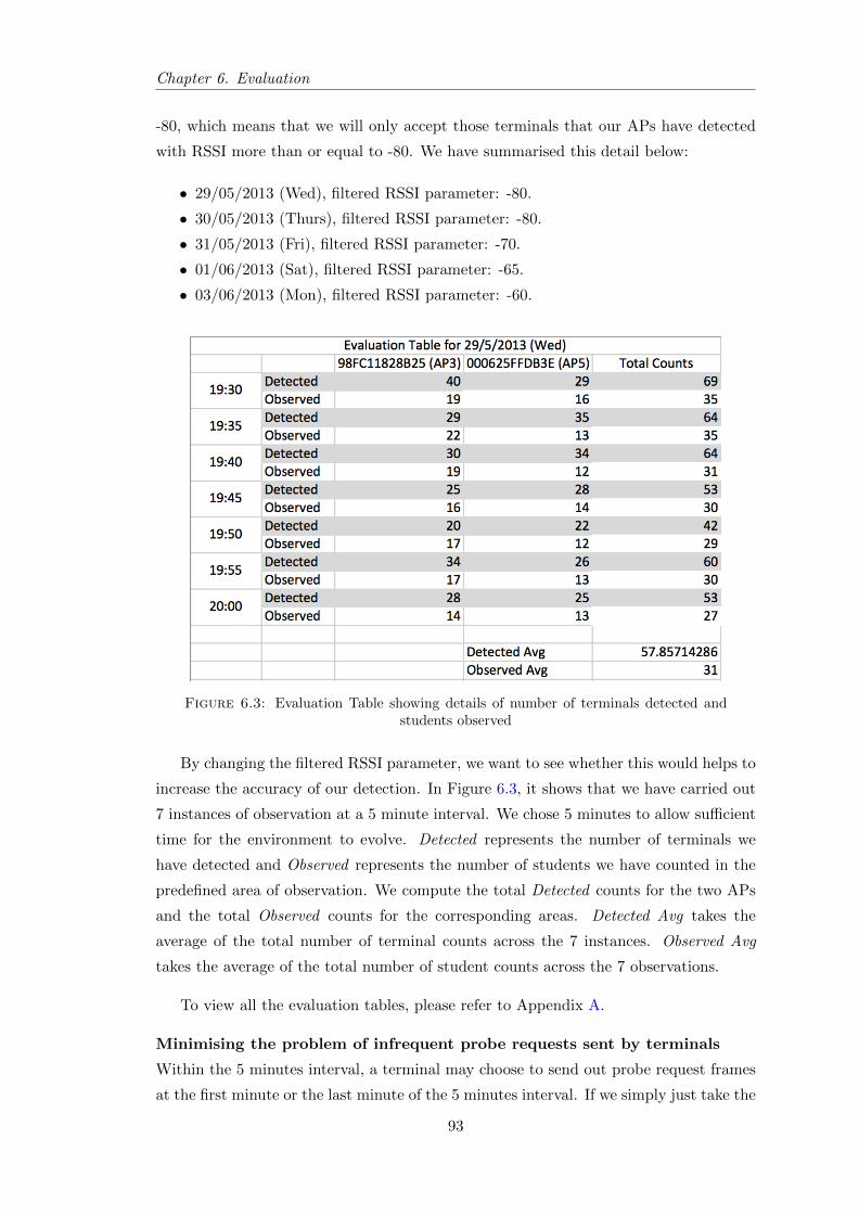
Chapter 6. Evaluation
-80, which means that we will only accept those terminals that our APs have detected
with RSSI more than or equal to -80. We have summarised this detail below:
• 29/05/2013 (Wed), filtered RSSI parameter: -80.
• 30/05/2013 (Thurs), filtered RSSI parameter: -80.
• 31/05/2013 (Fri), filtered RSSI parameter: -70.
• 01/06/2013 (Sat), filtered RSSI parameter: -65.
• 03/06/2013 (Mon), filtered RSSI parameter: -60.
Figure 6.3: Evaluation Table showing details of number of terminals detected andstudents observed
By changing the filtered RSSI parameter, we want to see whether this would helps to
increase the accuracy of our detection. In Figure 6.3, it shows that we have carried out
7 instances of observation at a 5 minute interval. We chose 5 minutes to allow sufficient
time for the environment to evolve. Detected represents the number of terminals we
have detected and Observed represents the number of students we have counted in the
predefined area of observation. We compute the total Detected counts for the two APs
and the total Observed counts for the corresponding areas. Detected Avg takes the
average of the total number of terminal counts across the 7 instances. Observed Avg
takes the average of the total number of student counts across the 7 observations.
To view all the evaluation tables, please refer to Appendix A.
Minimising the problem of infrequent probe requests sent by terminals
Within the 5 minutes interval, a terminal may choose to send out probe request frames
at the first minute or the last minute of the 5 minutes interval. If we simply just take the
93
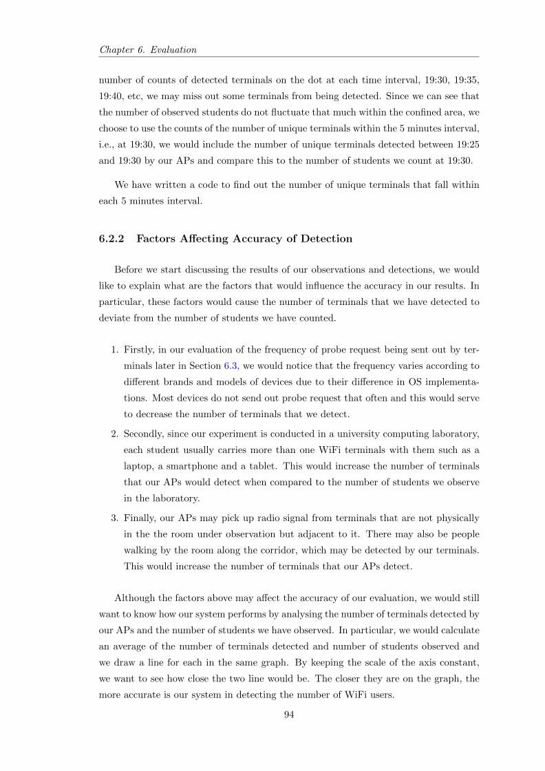
Chapter 6. Evaluation
number of counts of detected terminals on the dot at each time interval, 19:30, 19:35,
19:40, etc, we may miss out some terminals from being detected. Since we can see that
the number of observed students do not fluctuate that much within the confined area, we
choose to use the counts of the number of unique terminals within the 5 minutes interval,
i.e., at 19:30, we would include the number of unique terminals detected between 19:25
and 19:30 by our APs and compare this to the number of students we count at 19:30.
We have written a code to find out the number of unique terminals that fall within
each 5 minutes interval.
6.2.2 Factors Affecting Accuracy of Detection
Before we start discussing the results of our observations and detections, we would
like to explain what are the factors that would influence the accuracy in our results. In
particular, these factors would cause the number of terminals that we have detected to
deviate from the number of students we have counted.
1. Firstly, in our evaluation of the frequency of probe request being sent out by ter-
minals later in Section 6.3, we would notice that the frequency varies according to
different brands and models of devices due to their difference in OS implementa-
tions. Most devices do not send out probe request that often and this would serve
to decrease the number of terminals that we detect.
2. Secondly, since our experiment is conducted in a university computing laboratory,
each student usually carries more than one WiFi terminals with them such as a
laptop, a smartphone and a tablet. This would increase the number of terminals
that our APs would detect when compared to the number of students we observe
in the laboratory.
3. Finally, our APs may pick up radio signal from terminals that are not physically
in the the room under observation but adjacent to it. There may also be people
walking by the room along the corridor, which may be detected by our terminals.
This would increase the number of terminals that our APs detect.
Although the factors above may affect the accuracy of our evaluation, we would still
want to know how our system performs by analysing the number of terminals detected by
our APs and the number of students we have observed. In particular, we would calculate
an average of the number of terminals detected and number of students observed and
we draw a line for each in the same graph. By keeping the scale of the axis constant,
we want to see how close the two line would be. The closer they are on the graph, the
more accurate is our system in detecting the number of WiFi users.
94

Chapter 6. Evaluation
6.2.3 Discussion of Results
Across from Figure 6.4 to Figure 6.8, we can observed some trends from the graphs
plotted. It should be noted that the scale for x-axis and y-axis remains unchanged across
all the graphs. This would allow us to visually observe the change in trend across all
graphs.
First, let us compare the graph in Figure 6.4, which shows the count of the number
of terminals for 29/05/2013 (Wed) and Figure 6.5, for 30/05/2013 (Thurs). On these
two days, we keep the filtered RSSI parameter the same, i.e., at -80. What we can see
from the graphs of Detected Avg and Observed Avg reflects that filtered RSSI parame-
ter is crucial since this parameter causes these two graphs to shift up and down. The
ratio of Detected Avg to Observed Avg is 1.866 (calculated by 57.857/31) for 29/05/2013
and 1.887 (calculated by 52.285/27.714) for 30/05/2013. The ratios for both days re-
main almost unchanged, which indicates that by keeping the filtered RSSI parameter
unchanged, the accuracy of our detection would remain about the same too. Hence, it
also gives a good indication that no matter how the environment changes, as long as
the factors we have mentioned in Section 6.2.2 remain unchanged, our mechanism would
work as expected in detecting the number of terminals within the environment moni-
tored. Thus, it injects a great level of confidence that our aggregation process correctly
localises and counts the number of terminals.
Another very interesting trend that we observe across all graphs is as filtered RSSI
parameter increases from -80 to -70 and to -65, the Detected Avg and Observed Avg lines
become closer and closer, which indicates that our estimation of the actual number of
students in the confined area becomes more accurate up to this point. However, it should
be noted that on 01/06/2013, in which the filtered RSSI parameter was set at -65, it
was a Saturday and there were fewer number of students who came to the laboratory.
As the filtered RSSI parameter increases further to -60, which means that we ba-
sically filter out terminals with associated RSSI less than -60, we have reduced the
coverage that our APs would detect terminals. This actually has a negative effect and
does not bring the Detected Avg and Observed Avg lines close together.
There is one more trend which we can also observe across all graphs. From Figure
6.4 (29/05/2013) to Figure 6.7 (01/06/2013), the graphs of Detected and Detected Avg
are always above the graphs of Observed and Observed Avg. However, at one point when
we set the filtered RSSI parameter to -60, the opposite of what we have seen happens,
i.e., the graphs of Observed and Observed Avg are above the graphs of Detected and
Detected Avg as shown in Figure 6.8 instead. We know that filtered RSSI parameter of
-65 is actually the value that is suitable for our environment in the laboratory. From
95
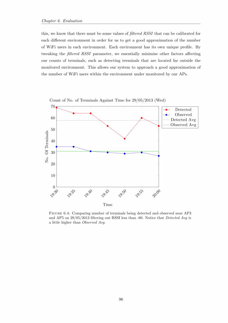
Chapter 6. Evaluation
this, we know that there must be some values of filtered RSSI that can be calibrated for
each different environment in order for us to get a good approximation of the number
of WiFi users in each environment. Each environment has its own unique profile. By
tweaking the filtered RSSI parameter, we essentially minimise other factors affecting
our counts of terminals, such as detecting terminals that are located far outside the
monitored environment. This allows our system to approach a good approximation of
the number of WiFi users within the environment under monitored by our APs.
19:30
19:35
19:40
19:45
19:50
19:55
20:00
0
10
20
30
40
50
60
70
Time
No.
Of
Ter
min
als
Count of No. of Terminals Against Time for 29/05/2013 (Wed)
DetectedObserved
Detected AvgObserved Avg
Figure 6.4: Comparing number of terminals being detected and observed near AP3and AP5 on 29/05/2013 filtering out RSSI less than -80. Notice that Detected Avg isa little higher than Observed Avg.
96

Chapter 6. Evaluation
19:30
19:35
19:40
19:45
19:50
19:55
20:00
0
10
20
30
40
50
60
70
Time
No.
Of
Ter
min
als
Count of No. of Terminals Against Time for 30/05/2013 (Thurs)
DetectedObserved
Detected AvgObserved Avg
Figure 6.5: Comparing number of terminals being detected and observed near AP3and AP5 on 30/05/2013 filtering out RSSI less than -80. Notice that Detected Avg isstill a little higher than Observed Avg.
11:30
11:35
11:40
11:45
11:50
11:55
12:00
0
10
20
30
40
50
60
70
Time
No.
Of
Ter
min
als
Count of No. of Terminals Against Time for 31/05/2013 (Fri)
DetectedObserved
Detected AvgObserved Avg
Figure 6.6: Comparing number of terminals being detected and observed near AP3and AP5 on 31/05/2013 filtering out RSSI less than -70. Notice that Detected Avg isgetting closer to Observed Avg.
97

Chapter 6. Evaluation
19:15
19:20
19:25
19:30
19:35
19:40
19:45
0
10
20
30
40
50
60
70
Time
No.
Of
Ter
min
als
Count of No. of Terminals Against Time for 01/06/2013 (Sat)
DetectedObserved
Detected AvgObserved Avg
Figure 6.7: Comparing number of terminals being detected and observed near AP3and AP5 on 01/06/2013 filtering out RSSI less than -65. Notice that Detected Avg isclosest to Observed Avg amongst all other graphs.
10:15
10:20
10:25
10:30
10:35
10:40
10:45
0
10
20
30
40
50
60
70
Time
No.
Of
Ter
min
als
Count of No. of Terminals Against Time for 03/06/2013 (Mon)
DetectedObserved
Detected AvgObserved Avg
Figure 6.8: Comparing number of terminals being detected and observed near AP3and AP5 on 03/06/2013 filtering out RSSI less than -60. Notice that Detected Avg isnow lower than Observed Avg instead.
98

Chapter 6. Evaluation
6.2.4 Analysing Trends from Web GUI
In Figure 6.9, we can observe a trend of the number of visitors in the laboratory.
We can see tht at around 12:45 and from 14:30 to 15:15, the number of visitors drop.
This indicates to us that these two periods are the most common periods that students
go out to have lunch. The peak of the histogram happens between 15:45 and 17:45,
indicating the peak period of the laboratory. This is true since we normally observe
that the laboratory is very packed around that time. Please note that the histogram in
the figure only shows the result for one AP. In the Web GUI, we can choose any AP to
view the statistics for it. Please refer to Section 5.6 for the URL and login details.
Figure 6.9: Trend of number of students in laboratory
6.3 Frequency of Probe Request Frames
Since we have collected so much data about WiFi devices, we could put it to good
use. We attempt to find out the average probe request frequency of major brands. We
want to know how often WiFi devices from each brand send out probe request frames.
This is probably the largest compilation of the frequency of probe request by carrying
out random sampling across the population of each brand. Previously, researchers would
measure the frequency of probe request of specific devices. This might not be a good
representation of a population of WiFi devices under each brand. We do recognise that
our results might not fully reflect the probe request frequency of each brand. However,
the results at least give us an idea of the general trend, in which we will analyse further
below.
99

Chapter 6. Evaluation
6.3.1 Compiling Process
Figure 6.10: Calculations of probe request frequency
In Figure 6.10, we have shown the table that we used to calculate the frequency
of probe request for each brand. First, we sort the detection records according to the
timestamp in ascending order and we only include those that we believe the terminal
still stay at the place it is being detected, i.e., our Residence Time algorithm has not
considered the terminal to have moved away somewhere else. Then we take the time the
terminal is first detected and the last time is it detected as shown in Figure 6.10. We
then count the number of records that exist between these two timestamps, n.
We use the formula below to determine the probe request frequency of each device.
last time detected− first time detected
n − 1
After this, we take the average across the number of samples we have for each brand.
We do recognise that the larger the number of samples, the better our representation
of the population. However, some brands of WiFi devices that we have detected have a
small population, hence, the sample size for each brand is different. This should be fine
since we classify each brand of devices as different population while we do our random
sampling, i.e., we randomly select devices for each brand.
We would like to thank MACVendorLookup [12] for providing the list of Organiza-
tionally Unique Identifier (OUI) that belongs to each manufacturer.
100
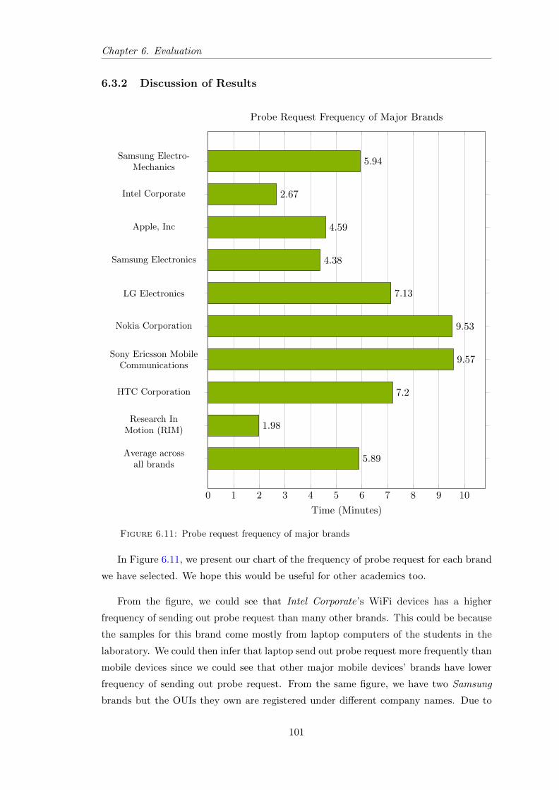
Chapter 6. Evaluation
6.3.2 Discussion of Results
0 1 2 3 4 5 6 7 8 9 10
Average acrossall brands
Research InMotion (RIM)
HTC Corporation
Sony Ericsson MobileCommunications
Nokia Corporation
LG Electronics
Samsung Electronics
Apple, Inc
Intel Corporate
Samsung Electro-Mechanics
5.89
1.98
7.2
9.57
9.53
7.13
4.38
4.59
2.67
5.94
Time (Minutes)
Probe Request Frequency of Major Brands
Figure 6.11: Probe request frequency of major brands
In Figure 6.11, we present our chart of the frequency of probe request for each brand
we have selected. We hope this would be useful for other academics too.
From the figure, we could see that Intel Corporate’s WiFi devices has a higher
frequency of sending out probe request than many other brands. This could be because
the samples for this brand come mostly from laptop computers of the students in the
laboratory. We could then infer that laptop send out probe request more frequently than
mobile devices since we could see that other major mobile devices’ brands have lower
frequency of sending out probe request. From the same figure, we have two Samsung
brands but the OUIs they own are registered under different company names. Due to
101
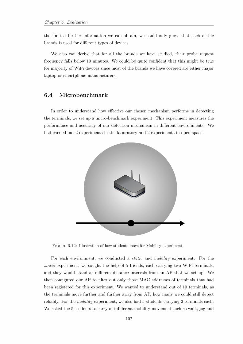
Chapter 6. Evaluation
the limited further information we can obtain, we could only guess that each of the
brands is used for different types of devices.
We also can derive that for all the brands we have studied, their probe request
frequency falls below 10 minutes. We could be quite confident that this might be true
for majority of WiFi devices since most of the brands we have covered are either major
laptop or smartphone manufacturers.
6.4 Microbenchmark
In order to understand how effective our chosen mechanism performs in detecting
the terminals, we set up a micro-benchmark experiment. This experiment measures the
performance and accuracy of our detection mechanism in different environments. We
had carried out 2 experiments in the laboratory and 2 experiments in open space.
Figure 6.12: Illustration of how students move for Mobility experiment
For each environment, we conducted a static and mobility experiment. For the
static experiment, we sought the help of 5 friends, each carrying two WiFi terminals,
and they would stand at different distance intervals from an AP that we set up. We
then configured our AP to filter out only those MAC addresses of terminals that had
been registered for this experiment. We wanted to understand out of 10 terminals, as
the terminals move further and further away from AP, how many we could still detect
reliably. For the mobility experiment, we also had 5 students carrying 2 terminals each.
We asked the 5 students to carry out different mobility movement such as walk, jog and
102
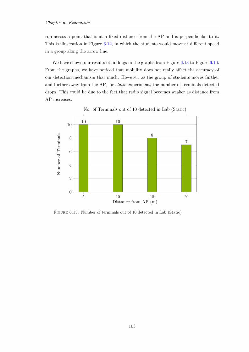
Chapter 6. Evaluation
run across a point that is at a fixed distance from the AP and is perpendicular to it.
This is illustration in Figure 6.12, in which the students would move at different speed
in a group along the arrow line.
We have shown our results of findings in the graphs from Figure 6.13 to Figure 6.16.
From the graphs, we have noticed that mobility does not really affect the accuracy of
our detection mechanism that much. However, as the group of students moves further
and further away from the AP, for static experiment, the number of terminals detected
drops. This could be due to the fact that radio signal becomes weaker as distance from
AP increases.
5 10 15 200
2
4
6
8
1010 10
8
7
Distance from AP (m)
Nu
mb
erof
Ter
min
als
No. of Terminals out of 10 detected in Lab (Static)
Figure 6.13: Number of terminals out of 10 detected in Lab (Static)
103
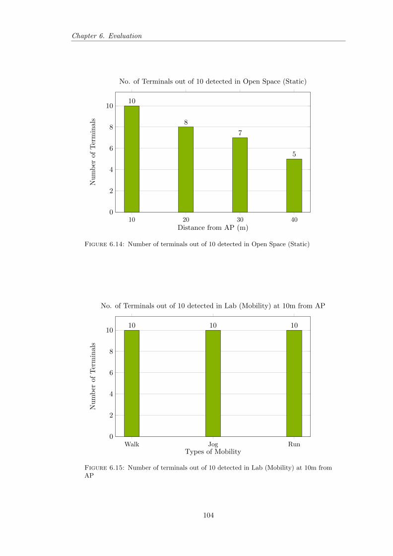
Chapter 6. Evaluation
10 20 30 400
2
4
6
8
1010
8
7
5
Distance from AP (m)
Nu
mb
erof
Ter
min
als
No. of Terminals out of 10 detected in Open Space (Static)
Figure 6.14: Number of terminals out of 10 detected in Open Space (Static)
Walk Jog Run0
2
4
6
8
1010 10 10
Types of Mobility
Nu
mb
erof
Ter
min
als
No. of Terminals out of 10 detected in Lab (Mobility) at 10m from AP
Figure 6.15: Number of terminals out of 10 detected in Lab (Mobility) at 10m fromAP
104
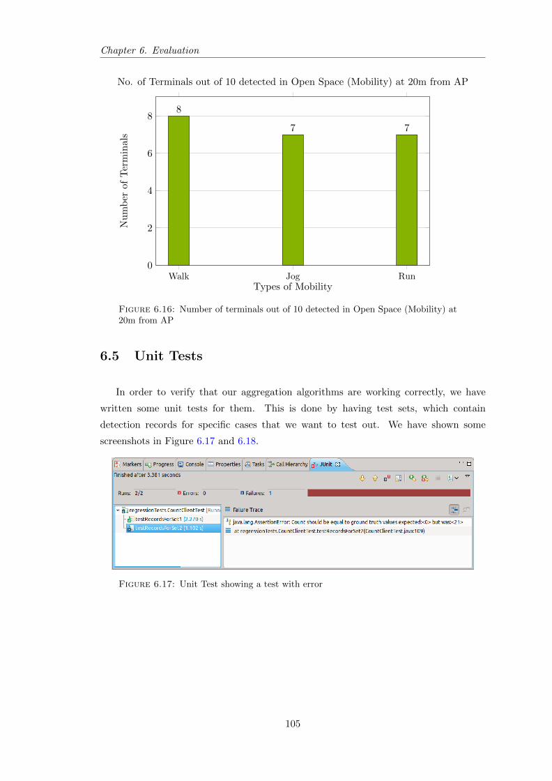
Chapter 6. Evaluation
Walk Jog Run0
2
4
6
88
7 7
Types of Mobility
Nu
mb
erof
Ter
min
als
No. of Terminals out of 10 detected in Open Space (Mobility) at 20m from AP
Figure 6.16: Number of terminals out of 10 detected in Open Space (Mobility) at20m from AP
6.5 Unit Tests
In order to verify that our aggregation algorithms are working correctly, we have
written some unit tests for them. This is done by having test sets, which contain
detection records for specific cases that we want to test out. We have shown some
screenshots in Figure 6.17 and 6.18.
Figure 6.17: Unit Test showing a test with error
105

Chapter 6. Evaluation
Figure 6.18: Unit Test showing a successful test
6.6 Summary
From the evaluation results that we have above, it shows that we have managed to
detect the presence of terminals, processed the collected data with the right logic and
displayed the results on a webpage. We have noticed that when we changed one of the
parameter of the experiment such as the filter RSSI value, this causes the ratio of the
number of terminals counted to the number of users observed to change as well.
The random sampling of probe request frequency as shown in Figure 6.11 gives us a
very good indication of the performance of our detection mechanism. The average probe
request frequency across all brands is 5.89 minutes, which suggests that our mechanism
has a tracking accuracy of around 5 minutes. This is good enough since we are not really
into tracking a specific user’s whereabouts but to track collective mobility of WiFi users
to understand a general trend and behaviour.
Finally, our micro-benchmark experiment put the sensitivity of our detection mech-
anism to test. The experiment indicates that our detection mechanism has a 100%
accuracy of detecting terminals that are 10m away from the AP, 80% for 20m, 70% for
30m and 50% for 40m in open space. As for the laboratory environment, which has
more interference, we have a detection accuracy of 100% for up to 10m of distance from
AP and 70% at a distance of 20m.
106
Chapter 7
Conclusion and Future Extensions
7.1 Conclusion
From detecting to aggregating and to displaying, each stage enables us to learn many
different aspects of computer science. We have dived into the lower level implementa-
tion of a program to run on an embedded device, employed the use of modern analytic
framework, MapReduce, and new breed of database, NoSQL, which has become ever
more popular due to the rise of Bigdata, and finally make use of the latest web technol-
ogy, HTML5, together with Javascript to create an app-like web interface experience.
Throughout the whole process, we learn and evaluate the suitability of each piece of
technology as well as understand their usage in big organisations by analysing relevant
case studies. This allows us to learn the best practice from these companies.
There are three main phases in this project. We began first by studying how different
WiFi components under the umbrella of IEEE 802.11 operate and communicate with
each other. Then we proposed a few different mechanisms that could be used to detect
the presence of WiFi terminals. We chose the best one, the detection of probe request
frames, that requires no actions to be taken from the users of the terminals while allowing
us to detect them passively. This mechanism was proven to work effectively in our
evaluation, in which we observed distinctive trend in the number of terminals detected
across the day in the laboratory, where we observed the period when students went out
for lunch break and the peak hours of the laboratory. Furthermore, the average number
of detected terminals were not too far away from the average number of students we
observed in the confined area. We provided reasons to explain the difference in the
number of terminals detected and number of users observed, as there are still limitations
in our project, which we could look into to extend in the future. This is discussed later
under Future Extensions.
While implementing the mechanism to detect terminals, we faced issues of flashing
the right firmware onto the AP and also the limitations in the computing resources of an
embedded device in terms of RAM and flash storage space. The cross compiling process
was the most rewarding one since it allowed us to successfully run our program on the
107
Chapter 7. Conclusion and Future Extensions
AP. If the compiling step did not succeed, we would have to look into alternative device
for implementation such as using a laptop with its NIC to simulate an AP.
In the second phase, we picked the most suitable method of aggregating the data
collected from each AP. At this phase, we managed to learn a lot about how to build
a collective representation of the mobility of WiFi users in a wireless network environ-
ment, using just the detection records we have, which compose of AP and terminal MAC
addresses, RSSI information and timestamp. These records are the fuel for our aggre-
gation engine, which makes use of the logic we have built into it to turn all this little
information into some meaningful statistics. It was also at this phase that we managed
to learn a lot more about the phenomenon we are faced with such as the “Ping Pong”
effect and the infrequent probe request broadcast. These phenomenons prompted us to
think further on how to fine tune our algorithms so that we could minimise the effect
of such problems. However, we do recognise that there is no easy way to increase the
frequency of probe request of terminals since that is dependant on the implementation
of the OS of the terminals.
In our final phase, although our aggregation engine could generate useful values, we
still have the task of visualising these values into something that human can comprehend.
We decided to build a web interface, which is the current most convenient way to browse
through information. Graphs and charts are plotted and drawn with colours and symbols
to explain what are going on at each AP. We managed to determine the number of
visitors located close to each AP, their residence time and the number of new and
returning visitors. Although this number does not actually represent the true number
of visitors, they give a good approximation to it since we could assume that most users
bring only one WiFi terminal either in their pocket or handbag when they are out in
shopping mall, supermarket or stadium. These are the places that our APs would most
likely be deployed in for a commercial roll-out.
7.2 Future Extensions
During our experiment, we observe a few phenomenons, which are real and need to
be addressed if we can extend this project further.
7.2.1 A More Reliable Way of Localising Terminal
We recognise that using just RSSI information to localising a terminal is not accurate
enough, which leads to the “Ping Pong” effect that we have mentioned earlier. After
108

Chapter 7. Conclusion and Future Extensions
reading through research papers and reviewing them under Related Work, we noticed
that there are various localisation techniques that could be employed to improve the
accuracy of localising a terminal. One such technique is triangulation, which requires
the use of 3 or more APs to detect and determine the position of a terminal.
7.2.2 Enclosing the Environment Under Monitored
Another issue that we noticed from our experiment is that, our APs are detecting
terminals that are outside the area that we are supposed to track. This contributes
to the inaccuracy that we may have in our statistics. In order to track the collective
mobility of users within a confined environment, we could develop techniques to ignore
users that are outside the confined space.
7.2.3 Ignoring Static Terminals
After our experiment, we also realised that there are WiFi terminals that just sit
there for hours and hours and there are no human carrying them. These terminals were
most likely be placed in the Computing Support Group room, which is located next
to the Common Room in which we have one AP deployed there for tracking terminals.
Furthermore, we also discovered a beautiful MAC address, 00:00:01:00:00:00, which
belongs to a Xerox brand, suggesting that it could be a printer having WiFi capability.
These devices should be ignored using appropriate technique.
7.2.4 Protecting Privacy of Individuals
Finally, throughout this project, we have been observing many different MAC ad-
dresses. Although we could not really pinpoint a MAC address to a person, unless the
person reveal this information, we would still like to enhance the privacy of individuals
that our system is tracking. This could be done by making use of a strong one-way hash
function with a salt to encrypt the MAC addresses. Whenever we detect a terminal’s
MAC address, we would hash it according to the hash function we have chosen and we
could still identify a unique terminal that we have detected before by comparing this
hashed values with the one we store in our database.
109

Appendix A
Evaluation Tables
Figure A.1: Evaluation tables for experiments on 29/05/2013 (Wed) and30/05/2013 (Thurs)
110
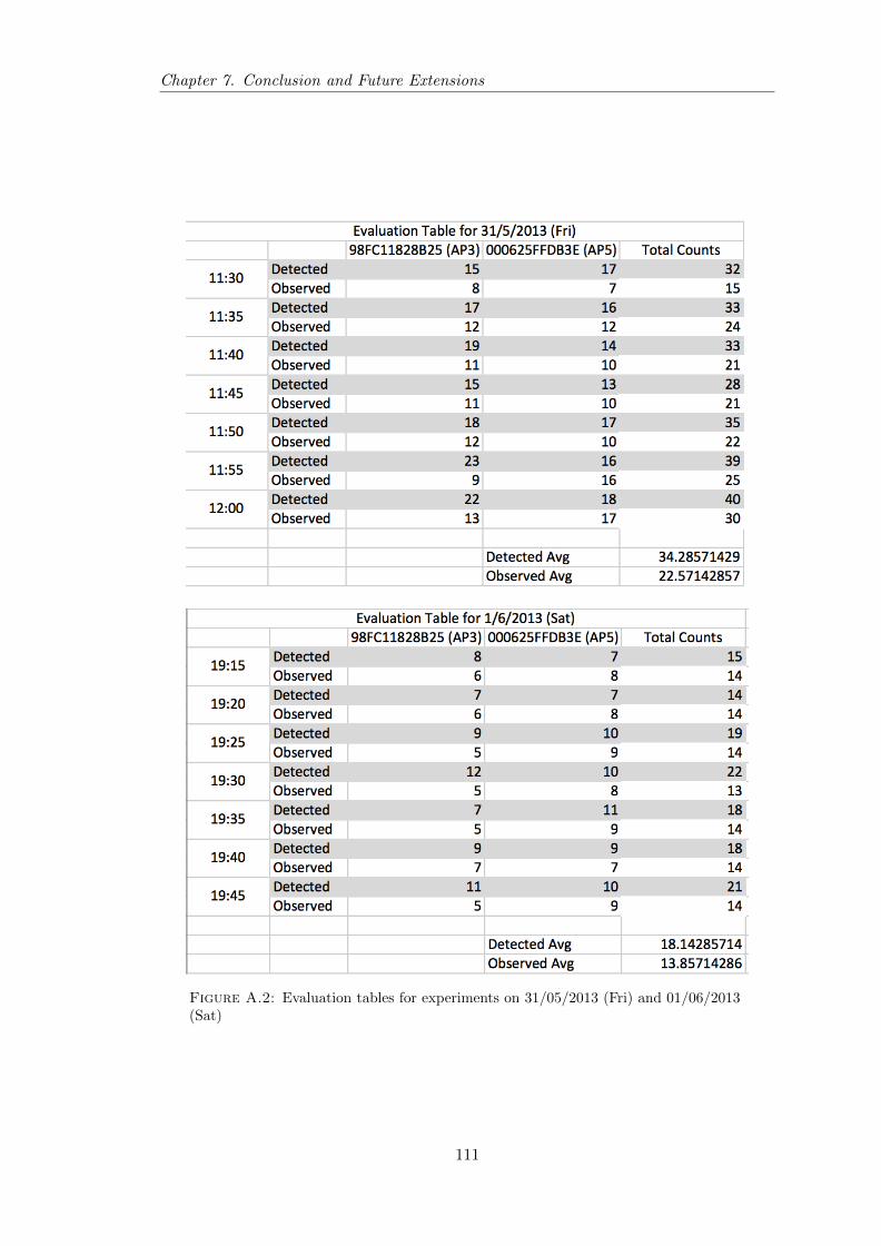
Chapter 7. Conclusion and Future Extensions
Figure A.2: Evaluation tables for experiments on 31/05/2013 (Fri) and 01/06/2013(Sat)
111

Chapter 7. Conclusion and Future Extensions
Figure A.3: Evaluation tables for experiments on 03/06/2013 (Mon)
112
Bibliography
[1] J.C. Anderson, J. Lehnardt, and N. Slater. CouchDB: The Definitive Guide. Animal
Guide Series. O’Reilly Media, 2010. ISBN 9780596155896.
[2] M. Azizyan, I. Constandache, and R. Roy Choudhury. Surroundsense: mobile
phone localization via ambience fingerprinting. Proceedings of the 15th annual in-
ternational conference on Mobile computing and networking, pages 261–272, 2009.
[3] DD-WRT Linux based Open Source firmware for Wireless routers and embedded
systems. URL http://dd-wrt.com.
[4] Broadcom. Broadcom Linux hybrid wireless driver. URL http://www.broadcom.
com/docs/linux_sta/README.txt. Accessed: 06/06/2013.
[5] Protocol Buffers. URL https://code.google.com/p/protobuf/. Accessed:
07/06/2013.
[6] Tom Carpenter. CWNA Certified Wireless Network Administrator Official Study
Guide: Exam PW0-100. Certification Press Series. McGraw-Hill Osborne Media,
2005. ISBN 9780072255386.
[7] Cisco. Channels and maximum power settings for cisco aironet autonomous access
points and bridges. October 2007. Pages 1-9 to 1-12.
[8] Cisco. 20 myths of wi-fi interference. pages 1–6, December 2007.
[9] Cisco. 802.11 network security fundamentals. 2008. Pages 1-2 to 1-4.
[10] WL Command. URL http://www.dd-wrt.com/wiki/index.php/WL. Accessed:
06/06/2013.
[11] cURL and libcurl. URL http://curl.haxx.se/docs/faq.html#What_is_
libcurl. Accessed: 07/06/2013.
[12] MAC Address OUI Vendor/Manufacturer Lookup Database. URL http://www.
macvendorlookup.com. Accessed: 15/06/2013.
[13] N. Dimiduk, A. Khurana, M.H. Ryan, and M. Stack. HBase in Action. Running
Series. Manning Publications Company, 2012. ISBN 9781617290527.
[14] OpenWrt Linux distribution for embedded devices. URL https://openwrt.org.
113

Bibliography
[15] Simple PHP Proxy: JavaScript finally ”gets” cross domain. URL http://
benalman.com/projects/php-simple-proxy. Accessed: 14/06/2013.
[16] Frequencies and Channels. Wikipedia. URL http://en.wikipedia.org/wiki/
IEEE_802.11#Frequencies_and_Channels. Accessed: 05/06/2013.
[17] Jim Geier. 802.11 Beacons Revealed. October 2002. URL http://www.
wi-fiplanet.com/tutorials/article.php/1492071. Accessed: 05/06/2013.
[18] L. George. HBase: The Definitive Guide. O’Reilly Media, 2011. ISBN
9781449315221.
[19] Minkyong Kim, David Kotz, and Songkuk Kim. Extracting a mobility model from
real user traces. INFOCOM 2006. 25th IEEE International Conference on Com-
puter Communications. Proceedings, pages 1–11, April 2006.
[20] Firmware Modification Kit. URL https://code.google.com/p/
firmware-mod-kit. Accessed: 11/06/2013.
[21] D. Kotz and K. Essien. Analysis of a campus-wide wireless network. Wireless
Networks, 11(1–2):115–133, 2005.
[22] libpcap. URL http://www.tcpdump.org/manpages/pcap.3pcap.html. Accessed:
06/06/2013.
[23] Kayle Miller. SNR, RSSI, EIRP and Free Space Path Loss. September 2010. URL
https://supportforums.cisco.com/docs/DOC-12954. Accessed: 05/06/2013.
[24] Wireless Operating Modes. URL http://wireless.kernel.org/en/users/
Documentation/modes. Accessed: 6/06/2013.
[25] Jan Newmarch. Data serialisation. URL http://jan.newmarch.name/go/
serialisation/chapter-serialisation.html. Accessed: 07/06/2013.
[26] Nanopb: protocol buffers with small code size. URL http://koti.kapsi.fi/jpa/
nanopb. Accessed: 07/06/2013.
[27] Wireless Setup. Archlinux. URL https://wiki.archlinux.org/index.php/
Wireless_Setup. Accessed: 06/06/2013.
[28] Bill Siwicki. More consumers access public wi-fi via mobile devices than lap-
tops. August 2012. URL http://www.internetretailer.com/2012/08/21/
more-access-public-wi-fi-mobile-devices-laptops. Accessed: 27/05/2013.
[29] “standards.”. Oxford University Press. 2013. URL http://oxforddictionaries.
com/definition/english/standard. Accessed: 04/06/2013.
114

Bibliography
[30] Apache Thrift. URL http://wiki.apache.org/thrift. Accessed: 14/06/2013.
[31] Unix time. Wikipedia. URL http://en.wikipedia.org/wiki/Unix_time. Ac-
cessed: 12/06/2013.
[32] Wiviz: Wireless Network Visualization. URL http://devices.natetrue.com/
wiviz. Accessed: 06/06/2013.
[33] CHRIS WEBB. Promise and Deferred objects in JavaScript Pt.1: The-
ory and Semantics. URL http://blog.mediumequalsmessage.com/
promise-deferred-objects-in-javascript-pt1-theory-and-semantics.
Accessed: 14/06/2013.
[34] Aaron Weiss. Introduction to Kismet. March 2006. URL http://www.
wi-fiplanet.com/tutorials/article.php/3595531. Accessed: 06/06/2013.
[35] Aaron Weiss. Introduction to NetStumbler. March 2006. URL http://www.
wi-fiplanet.com/tutorials/article.php/3589131. Accessed: 06/06/2013.
[36] T. White. Hadoop: The Definitive Guide: The Definitive Guide. O’Reilly Media,
2009. ISBN 9780596551360.
[37] Kismet: An 802.11 wireless network detector. URL http://www.kismetwireless.
net. Accessed: 11/06/2013.
[38] Wireshark. URL http://www.wireshark.org. Accessed: 06/06/2013.
115


![[PPT]What is IEEE 802.11 Doing?ieee802.org/11/Publicity/What is 802.11 doing.pptx · Web viewK – Radio Measurement P – Vehicular Environments R – Fast roaming S – MESH Networking](https://static.fdocuments.in/doc/165x107/5b8742527f8b9a162d8e9ed7/pptwhat-is-ieee-80211-doing-is-80211-doingpptx-web-viewk-radio-measurement.jpg)