User Localization using Random Access Channel Signals in ...
11
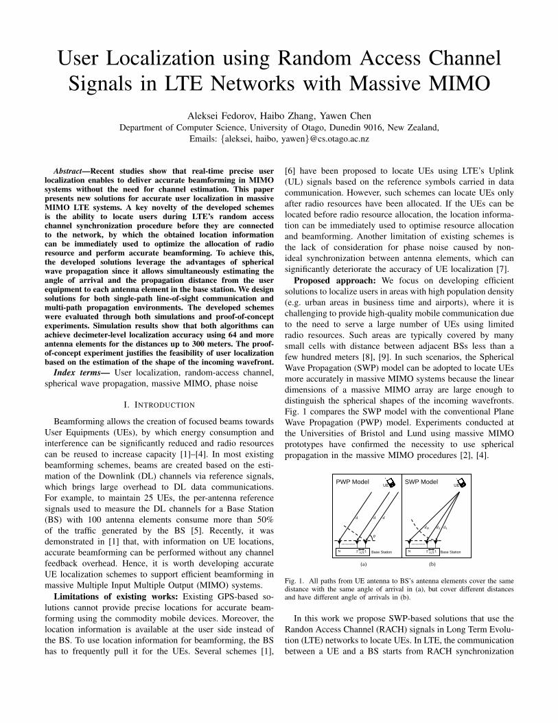
User Localization using Random Access Channel Signals in LTE Networks with Massive MIMO Fedorov, Aleksei; Zhang, Haibo; Chen, Yawen Published in: 2018 27th International Conference on Computer Communication and Networks (ICCCN) DOI: 10.1109/ICCCN.2018.8487359 2018 Document Version: Peer reviewed version (aka post-print) Link to publication Citation for published version (APA): Fedorov, A., Zhang, H., & Chen, Y. (2018). User Localization using Random Access Channel Signals in LTE Networks with Massive MIMO. In 2018 27th International Conference on Computer Communication and Networks (ICCCN) IEEE - Institute of Electrical and Electronics Engineers Inc.. https://doi.org/10.1109/ICCCN.2018.8487359 Total number of authors: 3 General rights Unless other specific re-use rights are stated the following general rights apply: Copyright and moral rights for the publications made accessible in the public portal are retained by the authors and/or other copyright owners and it is a condition of accessing publications that users recognise and abide by the legal requirements associated with these rights. • Users may download and print one copy of any publication from the public portal for the purpose of private study or research. • You may not further distribute the material or use it for any profit-making activity or commercial gain • You may freely distribute the URL identifying the publication in the public portal Read more about Creative commons licenses: https://creativecommons.org/licenses/ Take down policy If you believe that this document breaches copyright please contact us providing details, and we will remove access to the work immediately and investigate your claim.
Transcript of User Localization using Random Access Channel Signals in ...
LUND UNIVERSITY
PO Box 117221 00 Lund+46 46-222 00 00
User Localization using Random Access Channel Signals in LTE Networks withMassive MIMO
Fedorov, Aleksei; Zhang, Haibo; Chen, Yawen
Published in:2018 27th International Conference on Computer Communication and Networks (ICCCN)
DOI:10.1109/ICCCN.2018.8487359
2018
Document Version:Peer reviewed version (aka post-print)
Link to publication
Citation for published version (APA):Fedorov, A., Zhang, H., & Chen, Y. (2018). User Localization using Random Access Channel Signals in LTENetworks with Massive MIMO. In 2018 27th International Conference on Computer Communication andNetworks (ICCCN) IEEE - Institute of Electrical and Electronics Engineers Inc..https://doi.org/10.1109/ICCCN.2018.8487359
Total number of authors:3
General rightsUnless other specific re-use rights are stated the following general rights apply:Copyright and moral rights for the publications made accessible in the public portal are retained by the authorsand/or other copyright owners and it is a condition of accessing publications that users recognise and abide by thelegal requirements associated with these rights. • Users may download and print one copy of any publication from the public portal for the purpose of private studyor research. • You may not further distribute the material or use it for any profit-making activity or commercial gain • You may freely distribute the URL identifying the publication in the public portal
Read more about Creative commons licenses: https://creativecommons.org/licenses/Take down policyIf you believe that this document breaches copyright please contact us providing details, and we will removeaccess to the work immediately and investigate your claim.
User Localization using Random Access ChannelSignals in LTE Networks with Massive MIMO
Aleksei Fedorov, Haibo Zhang, Yawen ChenDepartment of Computer Science, University of Otago, Dunedin 9016, New Zealand,
Emails: {aleksei, haibo, yawen}@cs.otago.ac.nz
Abstract—Recent studies show that real-time precise userlocalization enables to deliver accurate beamforming in MIMOsystems without the need for channel estimation. This paperpresents new solutions for accurate user localization in massiveMIMO LTE systems. A key novelty of the developed schemesis the ability to locate users during LTE’s random accesschannel synchronization procedure before they are connectedto the network, by which the obtained location informationcan be immediately used to optimize the allocation of radioresource and perform accurate beamforming. To achieve this,the developed solutions leverage the advantages of sphericalwave propagation since it allows simultaneously estimating theangle of arrival and the propagation distance from the userequipment to each antenna element in the base station. We designsolutions for both single-path line-of-sight communication andmulti-path propagation environments. The developed schemeswere evaluated through both simulations and proof-of-conceptexperiments. Simulation results show that both algorithms canachieve decimeter-level localization accuracy using 64 and moreantenna elements for the distances up to 300 meters. The proof-of-concept experiment justifies the feasibility of user localizationbased on the estimation of the shape of the incoming wavefront.
Index terms— User localization, random-access channel,spherical wave propagation, massive MIMO, phase noise
I. INTRODUCTION
Beamforming allows the creation of focused beams towardsUser Equipments (UEs), by which energy consumption andinterference can be significantly reduced and radio resourcescan be reused to increase capacity [1]–[4]. In most existingbeamforming schemes, beams are created based on the esti-mation of the Downlink (DL) channels via reference signals,which brings large overhead to DL data communications.For example, to maintain 25 UEs, the per-antenna referencesignals used to measure the DL channels for a Base Station(BS) with 100 antenna elements consume more than 50%of the traffic generated by the BS [5]. Recently, it wasdemonstrated in [1] that, with information on UE locations,accurate beamforming can be performed without any channelfeedback overhead. Hence, it is worth developing accurateUE localization schemes to support efficient beamforming inmassive Multiple Input Multiple Output (MIMO) systems.
Limitations of existing works: Existing GPS-based so-lutions cannot provide precise locations for accurate beam-forming using the commodity mobile devices. Moreover, thelocation information is available at the user side instead ofthe BS. To use location information for beamforming, the BShas to frequently pull it for the UEs. Several schemes [1],
[6] have been proposed to locate UEs using LTE’s Uplink(UL) signals based on the reference symbols carried in datacommunication. However, such schemes can locate UEs onlyafter radio resources have been allocated. If the UEs can belocated before radio resource allocation, the location informa-tion can be immediately used to optimise resource allocationand beamforming. Another limitation of existing schemes isthe lack of consideration for phase noise caused by non-ideal synchronization between antenna elements, which cansignificantly deteriorate the accuracy of UE localization [7].
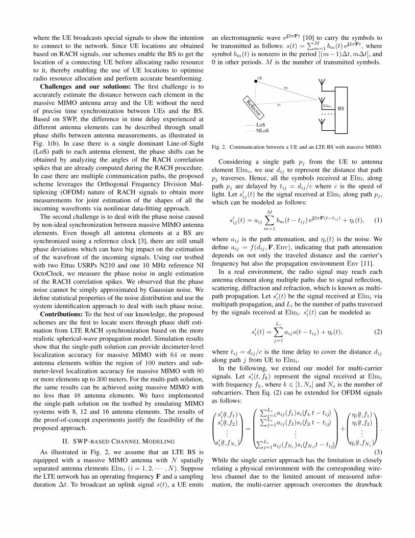
Proposed approach: We focus on developing efficientsolutions to localize users in areas with high population density(e.g. urban areas in business time and airports), where it ischallenging to provide high-quality mobile communication dueto the need to serve a large number of UEs using limitedradio resources. Such areas are typically covered by manysmall cells with distance between adjacent BSs less than afew hundred meters [8], [9]. In such scenarios, the SphericalWave Propagation (SWP) model can be adopted to locate UEsmore accurately in massive MIMO systems because the lineardimensions of a massive MIMO array are large enough todistinguish the spherical shapes of the incoming wavefronts.Fig. 1 compares the SWP model with the conventional PlaneWave Propagation (PWP) model. Experiments conducted atthe Universities of Bristol and Lund using massive MIMOprototypes have confirmed the necessity to use sphericalpropagation in the massive MIMO procedures [2], [4].
12 𝜆/2N
𝜃
UE
𝑑𝑑𝑑
12 𝜆/2N
UE
𝑑1𝑑2𝑑𝑁
Base Station Base Station
PWP Model SWP Model
(a) (b)
Fig. 1. All paths from UE antenna to BS’s antenna elements cover the samedistance with the same angle of arrival in (a), but cover different distancesand have different angle of arrivals in (b).
In this work we propose SWP-based solutions that use theRandon Access Channel (RACH) signals in Long Term Evolu-tion (LTE) networks to locate UEs. In LTE, the communicationbetween a UE and a BS starts from RACH synchronization
where the UE broadcasts special signals to show the intentionto connect to the network. Since UE locations are obtainedbased on RACH signals, our schemes enable the BS to get thelocation of a connecting UE before allocating radio resourceto it, thereby enabling the use of UE locations to optimiseradio resource allocation and perform accurate beamforming.
Challenges and our solutions: The first challenge is toaccurately estimate the distance between each element in themassive MIMO antenna array and the UE without the needof precise time synchronization between UEs and the BS.Based on SWP, the difference in time delay experienced atdifferent antenna elements can be described through smallphase shifts between antenna measurements, as illustrated inFig. 1(b). In case there is a single dominant Line-of-Sight(LoS) path to each antenna element, the phase shifts can beobtained by analyzing the angles of the RACH correlationspikes that are already computed during the RACH procedure.In case there are multiple communication paths, the proposedscheme leverages the Orthogonal Frequency Division Mul-tiplexing (OFDM) nature of RACH signals to obtain moremeasurements for joint estimation of the shapes of all theincoming wavefronts via nonlinear data-fitting approach.
The second challenge is to deal with the phase noise causedby non-ideal synchronization between massive MIMO antennaelements. Even though all antenna elements at a BS aresynchronized using a reference clock [3], there are still smallphase deviations which can have big impact on the estimationof the wavefront of the incoming signals. Using our testbedwith two Ettus USRPs N210 and one 10 MHz reference NIOctoClock, we measure the phase noise in angle estimationof the RACH correlation spikes. We observed that the phasenoise cannot be simply approximated by Gaussian noise. Wedefine statistical properties of the noise distribution and use thesystem identification approach to deal with such phase noise.
Contributions: To the best of our knowledge, the proposedschemes are the first to locate users through phase shift esti-mation from LTE RACH synchronization based on the morerealistic spherical-wave propagation model. Simulation resultsshow that the single-path solution can provide decimeter-levellocalization accuracy for massive MIMO with 64 or moreantenna elements within the region of 100 meters and sub-meter-level localization accuracy for massive MIMO with 80or more elements up to 300 meters. For the multi-path solution,the same results can be achieved using massive MIMO withno less than 48 antenna elements. We have implementedthe single-path solution on the testbed by emulating MIMOsystems with 8, 12 and 16 antenna elements. The results ofthe proof-of-concept experiments justify the feasibility of theproposed approach.
II. SWP-BASED CHANNEL MODELING
As illustrated in Fig. 2, we assume that an LTE BS isequipped with a massive MIMO antenna with N spatiallyseparated antenna elements Elmi (i = 1, 2, · · · , N). Supposethe LTE network has an operating frequency F and a samplingduration ∆t. To broadcast an uplink signal s(t), a UE emits
an electromagnetic wave ej2πFt [10] to carry the symbols tobe transmitted as follows: s(t) =
∑Mm=1 bm(t) ej2πFt, where
symbol bm(t) is nonzero in the period [(m−1)∆t,m∆t], and0 in other periods. M is the number of transmitted symbols.
time delay on subcarriers and reconstruct the time delay withnanosecond accuracy. However, unlike our method, they derivechannel model under the PWP assumption, which is unsuitablefor massive MIMO systems, and consequently cannot bedirectly implemented to massive MIMO.
The experiments with massive MIMO prototypes showedthe necessity of exploiting more realistic assumption basedon SWP [2]. The researchers from the University of Bristolclaimed that PWP is not suitable for massive MIMO systemsanymore. The theoretical comparison of channels generatedunder the two assumptions is provided in [8], where theauthors clearly showed that for antenna arrays with largeamount of antenna elements the difference between the twochannels becomes significant and this difference has to betaken into account. These results motivated us to developmethods that utilize SWP in UEs localization problem.
III. BACKGROUND ON LTE RACHTo connect to an LTE network, a UE has to perform the
RACH synchronization procedure by sending a RACH signal(i.e. preamble) to a network BS [10]. For this purpose, the UErandomly selects a RACH preamble from the assigned list ofavailable preambles, which is also known at the BS side, andsends it. Once the preamble reaches the BS, the correlationsbetween the incoming signal and the local preambles fromthe assigned list are calculated. If the incoming signal matcheswith a preamble in the assigned list, a correlation spike occurs.By detecting the correlation spike, the BS distinguishes theexact preamble used by a UE and estimates its time delay.
To improve the robustness of RACH synchronization,the preambles have to be created with good self- andmutual-orthogonality. RACH preambles are generated fromthe Zadoff-Chu (ZC) sequences [11], which have constantamplitude and zero autocorrelation waveforms. In the timedomain, a root ZC sequence is defined as follows:
zcu(l) = e�j
⇡ul(l+1)NZC , (1)
where NZC = 839, l = 0, . . . , NZC � 1, and the root indexu is a prime number less than NZC . Other sequences can begenerated by cyclically shifting the root sequence. The timedomain sequence is then converted to ZC(k) in the frequencydomain via an 839 points Discret Fourier Transform (DFT).
To generate a RACH signal in the time domain, the 839elements of ZC(k) are mapped to the assigned OFDM sub-carriers in the frequency domain and then converted to thetime domain via a 1024 points Inverse Fast Fourier Transform(IFFT). The UE performs upsampling of the obtained RACHsignal in order to mix with the carrier waveform and transmitsthe upsampled RACH signal to the BS. The sampling rateof the transmitted RACH signal becomes equivalent to theconventional sampling rate of the LTE system [10]. Thereverse steps done at the BS side start from removing carrierwaveform and downsampling to extract the ZC sequence ata lower sampling rate in digital time domain. The extractedsignal, actually, accumulates all the information about thechannel through which it has been transmitted. This channel
information can be used to find the location of the transmittingUE.
IV. SWP-BASED CHANNEL MODELLING
As illustrated in Fig. 1, we assume that an LTE BS isequipped with a massive MIMO antenna with N spatiallyseparated antenna elements Elmi (i = 1, 2, · · · , N). Supposethe LTE network has an operating frequency F and a samplingduration �t. To broadcast an uplink signal s(t), a UE emitsan electromagnetic wave ej2⇡Ft [12] to carry the symbols tobe transmitted as follows: s(t) =
PMm=1 bm(t) ej2⇡Ft, where
symbol bm(t) is 1 in the period [(m � 1)�t, m�t], and 0 inother periods. M is the number of transmitted symbols.
UE
BSElmi
Reflector
LoSNLoS
pk
pl
Fig. 1. Communication between a UE and a LTE BS with massive MIMO.
Consider a single path pj from the UE to antenna elementElmi, we use dij to represent the distance that path pj
traverses. Hence, all the symbols received at Elmi along pathpj are delayed by tij = dij/c where c is the speed of light.Let s0ij(t) be the signal received at Elmi along path pj , whichcan be modeled as follows:
s0ij(t) = aij
MX
m=1
bm(t � tij) ej2⇡F(t�tij) + ⌘i(t), (2)
where aij is the path attenuation, and ⌘i(t) is the noise. Wedefine aij = f(dij ,F, Env), indicating that path attenuationdepends on not only the traveled distance and the carrier’sfrequency but also the propagation environment Env [13].
In a real environment, the radio signal may reach eachantenna element along multiple paths due to signal reflection,scattering, diffraction and refraction, which is known as multi-path propagation. Let s0i(t) be the signal received at Elmi viamultipath propagation, and Li be the number of paths traversedby the signals received at Elmi. s0i(t) can be modelled as
s0i(t) =
LiX
j=1
aijs(t � tij) + ⌘i(t), (3)
where tij = dij/c is the time delay to cover the distance dij
along path j from UE to Elmi.The above wireless channels are modelled based on single
carrier signal. However, LTE uses OFDM that is based onmulti-carrier modulation. In the following we extend ourmodel for multi-carrier signals. Let s0i(t, fk) represent thesignal received at Elmi with frequency fk, where sk(t) is
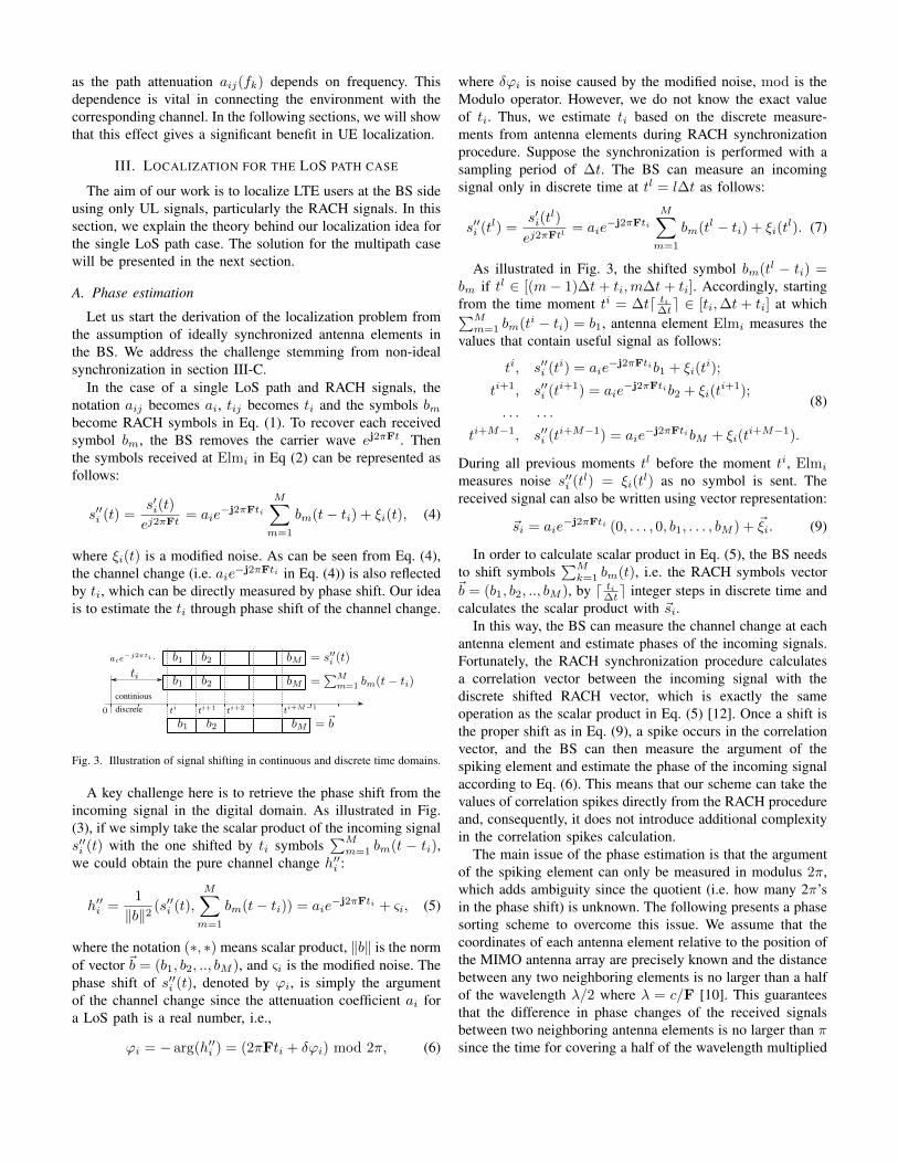
Fig. 2. Communication between a UE and an LTE BS with massive MIMO.
Considering a single path pj from the UE to antennaelement Elmi, we use dij to represent the distance that pathpj traverses. Hence, all the symbols received at Elmi alongpath pj are delayed by tij = dij/c where c is the speed oflight. Let s′ij(t) be the signal received at Elmi along path pj ,which can be modeled as follows:
s′ij(t) = aij
M∑
m=1
bm(t− tij) ej2πF(t−tij) + ηi(t), (1)
where aij is the path attenuation, and ηi(t) is the noise. Wedefine aij = f(dij ,F,Env), indicating that path attenuationdepends on not only the traveled distance and the carrier’sfrequency but also the propagation environment Env [11].
In a real environment, the radio signal may reach eachantenna element along multiple paths due to signal reflection,scattering, diffraction and refraction, which is known as multi-path propagation. Let s′i(t) be the signal received at Elmi viamultipath propagation, and Li be the number of paths traversedby the signals received at Elmi. s′i(t) can be modeled as
s′i(t) =
Li∑
j=1
aijs(t− tij) + ηi(t), (2)
where tij = dij/c is the time delay to cover the distance dijalong path j from UE to Elmi.
In the following, we extend our model for multi-carriersignals. Let s′i(t, fk) represent the signal received at Elmi
with frequency fk, where k ∈ [1, Ns] and Ns is the number ofsubcarriers. Then Eq. (2) can be extended for OFDM signalsas follows:
s′i(t,f1)s′i(t,f2)
...s′i(t,fNs)
=
∑Lij=1aij(f1)si(f1, t− tij)∑Lij=1aij(f2)si(f2, t− tij)
...∑Lij=1aij(fNs)si(fNs,t− tij)
+
ηi(t,f1)ηi(t,f2)
...ηi(t,fNs)
.
(3)While the single carrier approach has the limitation in closelyrelating a physical environment with the corresponding wire-less channel due to the limited amount of measured infor-mation, the multi-carrier approach overcomes the drawback
as the path attenuation aij(fk) depends on frequency. Thisdependence is vital in connecting the environment with thecorresponding channel. In the following sections, we will showthat this effect gives a significant benefit in UE localization.
III. LOCALIZATION FOR THE LOS PATH CASE
The aim of our work is to localize LTE users at the BS sideusing only UL signals, particularly the RACH signals. In thissection, we explain the theory behind our localization idea forthe single LoS path case. The solution for the multipath casewill be presented in the next section.
A. Phase estimation
Let us start the derivation of the localization problem fromthe assumption of ideally synchronized antenna elements inthe BS. We address the challenge stemming from non-idealsynchronization in section III-C.
In the case of a single LoS path and RACH signals, thenotation aij becomes ai, tij becomes ti and the symbols bmbecome RACH symbols in Eq. (1). To recover each receivedsymbol bm, the BS removes the carrier wave ej2πFt. Thenthe symbols received at Elmi in Eq (2) can be represented asfollows:
s′′i (t) =s′i(t)ej2πFt
= aie−j2πFti
M∑
m=1
bm(t− ti) + ξi(t), (4)
where ξi(t) is a modified noise. As can be seen from Eq. (4),the channel change (i.e. aie−j2πFti in Eq. (4)) is also reflectedby ti, which can be directly measured by phase shift. Our ideais to estimate the ti through phase shift of the channel change.
While the single carrier approach has the limitation in closelyrelating a physical environment with the corresponding wire-less channel due to the limited amount of measured infor-mation, the multi-carrier approach overcomes the drawbackas the path attenuation aij(fk) depends on frequency. Thisdependence is vital in connecting of the environment with thecorresponding channel. In the following sections, we will showthat this effect gives a significant benefit in UE localization.
VI. LOCALISATION FOR THE LOS PATH CASE
The aim of our work is to localize LTE users at the BSside using only UL signals, particularly the RACH signals.With a massive MIMO antenna, this becomes feasible since thesignal measurements at the antenna elements become enoughto jointly estimate the locations of UEs. In this section weexplain the theory behind our localization idea for the singleLine-of-Sight (LoS) path case. The solution for the multipathcase will be presented in the next section.
A. Phase estimation
We assume that all antenna elements of the BS are wellsynchronized since they share a common local oscillator andcan be pre-synchronized for phase alignment [?]. Since weonly consider the LoS path, the notation aij becomes ai, andtij becomes ti. To recover each received symbol bm, the BSremoves the carrier wave ej2⇡Ft. Then the symbols receivedat Elmi based on Eq (3) can be represented as follows:
s00i (t) =s0i(t)
ej2⇡Ft= aie
�j2⇡Fti
MX
m=1
bm(t � ti) + ⇠i(t), (5)
where ⇠i(t) is a modified noise.
0
b1 b2 bMaie�j2⇡ti ·
continiousdiscrete ti ti+1 ti+2 ti+M�1
b1 b2 bM
b1 b2 bM
ti
= s00i (t)
=PM
m=1 bm(t � ti)
= ~b
Fig. 2. Signal’s reception and its representation in continuous and discretetime domains.
A key challenge here is to measure the phase of an incomingsignal in the digital domain. As illustrated in Fig. 2, we simplytake the scalar product of the incoming signal s00i (t) with theone shifted by ti symbols
PMm=1 bm(t�tij) to obtain the pure
channel change h0i:
h00i =
1
kbk2(s00i (t),
MX
m=1
bm(t � ti)) = aie�j2⇡Fti + &i, (6)
where kbk is the norm of vector b = (b1, b2, .., bM ), and&i is the modified noise. The phase of s00i (t), denoted by'i, is simply the argument of the channel change since theattenuation coefficient ai for a LoS path is a real number, i.e.,
'i = � arg(h00i ) = 2⇡Fti mod 2⇡, (7)
where mod is the Modulo operator. Note that the influenceof &i to the phase estimation is considered as minuscule sincethe standard deviation of the phase change caused by &i, evenfor zero SNR, is less than 1/kbk2 (1/839 in LTE [?]).
Since the computation of 'i needs the knowledge of ti,we estimate ti based on the discrete measurements fromantenna elements during RACH synchronization. Suppose LTEoperates with a sampling period of �t. The BS can measure anincoming signal only in discrete time at tl = l�t as follows:
s00i (tl) =s0i(t
l)
ej2⇡Ftl = aie�j2⇡Fti
MX
m=1
bm(tl � ti) + ⇠i(tl). (8)
As illustrated in Fig. 2, the shifted symbol bm(tl � ti) =bm if tl 2 [(m � 1)�t + ti, m�t + ti]. Accordingly, startingfrom the time moment ti = �td ti
�te 2 [ti,�t + ti] at whichPMm=1 bm(ti � ti) = b1, antenna element Elmi measures the
values that contain useful signal as follows:
ti, s00i (ti) = aie�j2⇡Ftib1 + ⇠i(t
i);
ti+1, s00i (ti+1) = aie�j2⇡Ftib2 + ⇠i(t
i+1);
. . . . . .
ti+M�1, s00i (ti+M�1) = aie�j2⇡FtibM + ⇠i(t
i+M�1).
(9)
During all previous moments tl before the moment ti, Elmi
measures noise s00i (tl) = ⇠i(tl) as no symbol is sent. The
received signal can also be written using vector representation:
~si = aije�j2⇡Fti (0, . . . , 0, b1, . . . , bM ) + ~⇠i. (10)
In order to the calculate scalar product in Eq. (6), the BSneeds to shift symbols
PMk=1 bm(t), i.e. the RACH preamble
vector ~b = (b1, b2, .., bM ), by d ti
�te integer steps in discretetime and calculates the scalar product with ~si. In this way, theBS can measure the channel change at each antenna element,and estimate phases of the incoming signals. Fortunately,the RACH synchronization procedure calculates a correlationvector between the incoming signal with the discrete shiftedpreamble vector, which is exactly the same operation as thescalar product in Eq. (6) [13]. Once a shift is the proper shiftas in Eq. (10), a spike occurs in the correlation vector, andthe BS can then measure the argument of the spiking elementand estimate the phase of the incoming signal according toEq. (7). The main issue of this procedure is that the argumentof the spiking element can only be measured in modulus 2⇡,which adds ambiguity since the quotient (i.e. how many 2⇡’sin the phase shift) is unknown. In the following we present ascheme based on phase sorting to overcome this issue.
We assume that the coordinates of each antenna elementrelative to the position of the MIMO antenna array is preciselyknown and the distance between any two neighboring elementsis no larger than a half of the wavelength �/2 where � = c/F[11]. This guarantee that the difference in phase changesof the received signals between two neighboring antennaelements is no larger than ⇡ since the time for covering ahalf of the wavelength multiplied to the frequency in radiansis �
2c ⇥ 2⇡F = ⇡. Consequently, for any two neighboring
Fig. 3. Illustration of signal shifting in continuous and discrete time domains.
A key challenge here is to retrieve the phase shift from theincoming signal in the digital domain. As illustrated in Fig.(3), if we simply take the scalar product of the incoming signals′′i (t) with the one shifted by ti symbols
∑Mm=1 bm(t − ti),
we could obtain the pure channel change h′′i :
h′′i =1
‖b‖2 (s′′i (t),
M∑
m=1
bm(t− ti)) = aie−j2πFti + ςi, (5)
where the notation (∗, ∗) means scalar product, ‖b‖ is the normof vector ~b = (b1, b2, .., bM ), and ςi is the modified noise. Thephase shift of s′′i (t), denoted by ϕi, is simply the argumentof the channel change since the attenuation coefficient ai fora LoS path is a real number, i.e.,
ϕi = − arg(h′′i ) = (2πFti + δϕi) mod 2π, (6)
where δϕi is noise caused by the modified noise, mod is theModulo operator. However, we do not know the exact valueof ti. Thus, we estimate ti based on the discrete measure-ments from antenna elements during RACH synchronizationprocedure. Suppose the synchronization is performed with asampling period of ∆t. The BS can measure an incomingsignal only in discrete time at tl = l∆t as follows:
s′′i (tl) =s′i(t
l)
ej2πFtl= aie
−j2πFtiM∑
m=1
bm(tl − ti) + ξi(tl). (7)
As illustrated in Fig. 3, the shifted symbol bm(tl − ti) =bm if tl ∈ [(m − 1)∆t + ti,m∆t + ti]. Accordingly, startingfrom the time moment ti = ∆td ti∆te ∈ [ti,∆t + ti] at which∑Mm=1 bm(ti − ti) = b1, antenna element Elmi measures the
values that contain useful signal as follows:
ti, s′′i (ti) = aie−j2πFtib1 + ξi(t
i);
ti+1, s′′i (ti+1) = aie−j2πFtib2 + ξi(t
i+1);
. . . . . .
ti+M−1, s′′i (ti+M−1) = aie−j2πFtibM + ξi(t
i+M−1).
(8)
During all previous moments tl before the moment ti, Elmi
measures noise s′′i (tl) = ξi(tl) as no symbol is sent. The
received signal can also be written using vector representation:
~si = aie−j2πFti (0, . . . , 0, b1, . . . , bM ) + ~ξi. (9)
In order to calculate scalar product in Eq. (5), the BS needsto shift symbols
∑Mk=1 bm(t), i.e. the RACH symbols vector
~b = (b1, b2, .., bM ), by d ti∆te integer steps in discrete time andcalculates the scalar product with ~si.
In this way, the BS can measure the channel change at eachantenna element and estimate phases of the incoming signals.Fortunately, the RACH synchronization procedure calculatesa correlation vector between the incoming signal with thediscrete shifted RACH vector, which is exactly the sameoperation as the scalar product in Eq. (5) [12]. Once a shift isthe proper shift as in Eq. (9), a spike occurs in the correlationvector, and the BS can then measure the argument of thespiking element and estimate the phase of the incoming signalaccording to Eq. (6). This means that our scheme can take thevalues of correlation spikes directly from the RACH procedureand, consequently, it does not introduce additional complexityin the correlation spikes calculation.
The main issue of the phase estimation is that the argumentof the spiking element can only be measured in modulus 2π,which adds ambiguity since the quotient (i.e. how many 2π’sin the phase shift) is unknown. The following presents a phasesorting scheme to overcome this issue. We assume that thecoordinates of each antenna element relative to the position ofthe MIMO antenna array are precisely known and the distancebetween any two neighboring elements is no larger than a halfof the wavelength λ/2 where λ = c/F [10]. This guaranteesthat the difference in phase changes of the received signalsbetween two neighboring antenna elements is no larger than πsince the time for covering a half of the wavelength multiplied
to the frequency in radians is λ2c × 2πF = π. Consequently,
for any two neighboring antenna elements, the signal with thesmallest phase can be always found except in the situationwhere the difference is equal to π. This case is not consideredbecause the signals are in fact transmitted exactly from thedirection alongside the neighboring elements. In practice, suchsituation is very unlikely since a BS maintains a particulararea, which cancels situations with phase shift in close to πradians. The influence of noise δϕi can also be neglected in thephase sorting scheme since even in the situation with zero SNRRACH signals, the standard deviation is less than 0.03 radians.Consequently, for any two neighboring antenna elements, thesignal with smaller phase can be always found based on thefollowing two rules:• if |ϕi+1−ϕi| < π, the smaller one remains to be smaller
than the bigger one;• if |ϕi+1−ϕi| > π, the smaller one becomes bigger since
the difference between them cannot be bigger than π, and2π should be added to the smaller phase.
antenna elements, the signal with the smallest phase can bealways found except in the situation where the difference isequal to ⇡. This case is not considered because the signalsare in fact transmitted exactly from the direction alongsidethe neighboring elements. In practice, such the situation isvery unlikely since a BS maintains a particular area, whichcancels situations with phase shift in ⇡ radians. Consequently,for any two neighboring antenna elements, the signal withsmaller phase can be always found based on the followingtwo rules:
• if |'i+1�'i| < ⇡, the smaller one remains to be smallerthan the bigger one;
• if |'i+1�'i| > ⇡, the smaller one becomes bigger sincethe difference between them cannot be bigger than ⇡, and2⇡ should be added to the smaller phase.
UE
BS'i+1 = 10⇡6
Im
Re
'i = ⇡6
7
3
ElmiElmi�1 Elmi+1
(a) (b)
'i+1
'i+211.1⇡6
'i�1
11⇡6
0.1⇡6
0.4⇡6
'i
Fig. 3. The phase rotation according to antenna elements.
As illustrated in Fig. 3(a), 'i = ⇡6 and 'i+1 = 10⇡
6 . Since|'i+1�'i| > ⇡, the actual difference should be 2⇡+ ⇡
6 � 10⇡6 ,
i.e. the difference represented by the arrrow with solid lineinstead of the one with the dashed line. Hence, 'i > 'i+1.
To compute the actual phase for the signal received at eachantenna element, we need to find the minimum phase for thesignals received at all antenna elements, which can be doneby performing pairwise comparison between neighbouringantenna elements based on the above two rules. Suppose thesignal received at antenna element Elmi has the minimumphase 'i. For each neighbour of Elmi denoted by Elmj , if|'j�'i| > ⇡, 'j = 'j+2⇡; otherwise 'j remains unchanged.We repeat the same operation for the neighbours of Elmj andso on until all 'is have been corrected. As illustrated in Fig.3(b), the minimum phase is 'i = 11⇡
6 . Since |'i+1�'i| < ⇡,'i+1 remains unchanged. But for 'i+2, |'i+2 � 'i+1| > ⇡.Hence, 'i+2 = 0.1⇡
6 +2⇡ = 12.1⇡6 . In such a way the ambiguity
caused by unknown quotient is eliminated.
B. LoS localization during RACH synchronization
Because of the use of SWP, each phase shift 'i correspondsto a certain distance Ri = �⇥ 'i
2⇡ .As shown in Fig. 4, for each antenna element Elmi, we draw
a sphere centered at Elmi with radius of Ri. We further drawa sphere centred at the UE with radius of R = 2⇡N� so thatthis sphere is tangent to each sphere centred at Elmi wherei 2 [1, N ]. It can be seen that the LoS distance from the UE to
2⇡N�
'1
'2
'N
Im
Re
Re
Re
UE(x, y, z)
BS
Elm1
Elm2
ElmN
RN
R2
R1
'1
'2
'N
Fig. 4. The phase rotation alongside the antenna array.
antenna element Elmi can be rewritten by di = R + Ri, i =1, . . . , N . By representing di with the coordinates of the UE(x, y, z) and Elmi (xi, yi, zi), we have
p(x � xi)2 + (y � yi)2 + (z � zi)2 = R + Ri. (11)
To localize the UE, the BS needs to jointly estimate the UE’scoordinates and the common parameter N�. Since the numberof unknown parameters is four (x, y, z, R), the coordinates ofthe UE can be calculated if there are no less than 4 antennaelements, which is not a problem for BS with Massive MIMO[2], [?]. Once the BS has enough antenna elements, the aboveformulated localisation problem transforms to the classicalGNSS positioning problem that can be solved using Bancroft’salgorithm, which has a closed form solution [14].
C. Localization in the presence of carrier frequency offset
While the elements in one antenna array can be accuratelysynchronised as they share the same oscillator, the UEsand BSs have independent local oscillators, and cannot beideally synchronized. Consequently, there are always a CarrierFrequency Offset (CFO) �F, and a phase offset � caused bydifferent starting moments of the oscillators. This non-idealitycan be counted at the BS side in Eq. (8) as follows:
s00i (tl) =s0i(t
l)
ej⇥2⇡(F��F)tl��
⇤ =
= aie�j2⇡Fti
ej�
MX
m=1
bm(tl � ti)ej2⇡�F tl
�+ ⇠i(t
l). (12)
In the same way as in (9), the useful signal starts to reach Elmi
at moment ti, and the vector representation of the receivedsignal given in Eq. (10) can be rewritten as follows:
~si = Kiej� (0, . . . , 0, b1f
i, . . . , bM fi+M�1) + ~⇠i, (13)
where fi = ej2⇡�F ti
and Ki = aie�j2⇡Fti . Hence, the spiking
value in the correlation vector between the incoming signaland RACH preamble vector ~b can be represented as:
h0i = aie
�j2⇡Fti
ej� 1
kbk2
MX
m=1
f i+m�1
�+ &i. (14)
Fig. 4. Phase shift at different antenna elements.
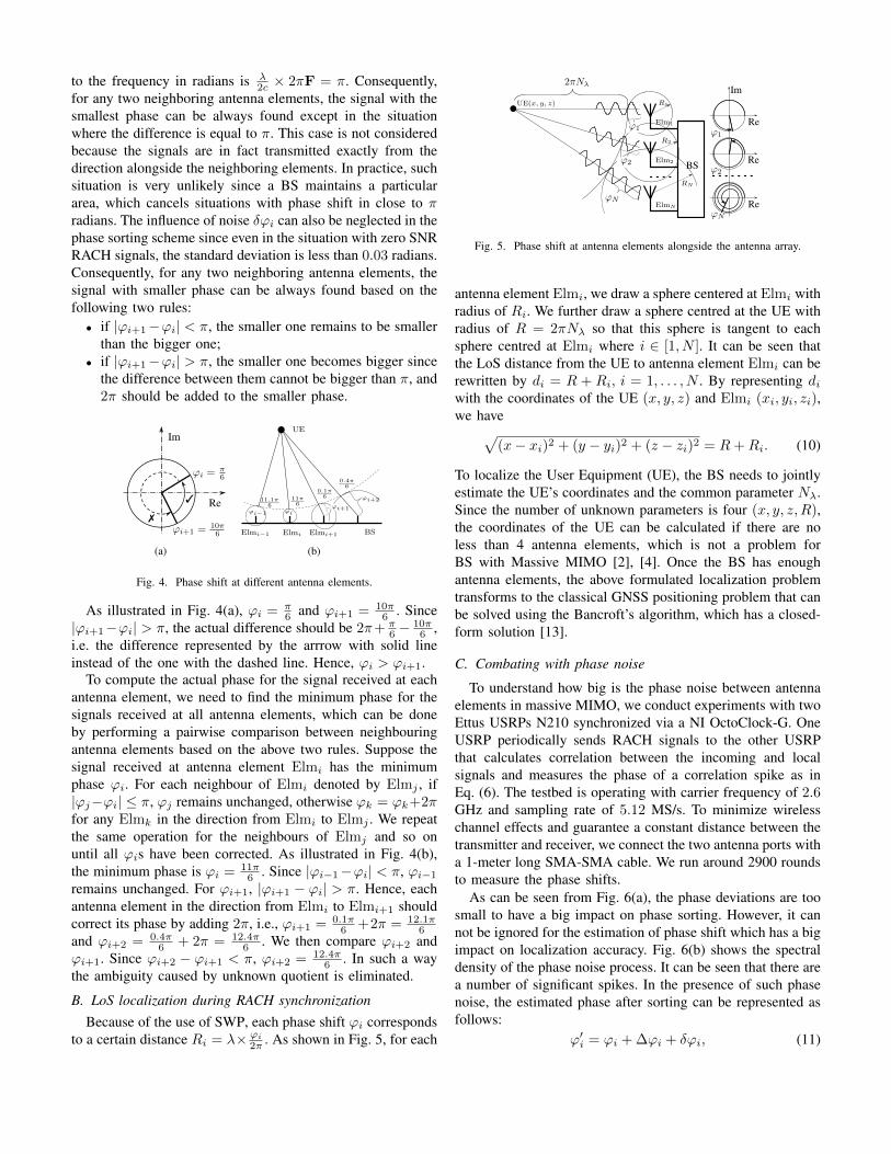
As illustrated in Fig. 4(a), ϕi = π6 and ϕi+1 = 10π
6 . Since|ϕi+1−ϕi| > π, the actual difference should be 2π+ π
6 − 10π6 ,
i.e. the difference represented by the arrrow with solid lineinstead of the one with the dashed line. Hence, ϕi > ϕi+1.
To compute the actual phase for the signal received at eachantenna element, we need to find the minimum phase for thesignals received at all antenna elements, which can be doneby performing a pairwise comparison between neighbouringantenna elements based on the above two rules. Suppose thesignal received at antenna element Elmi has the minimumphase ϕi. For each neighbour of Elmi denoted by Elmj , if|ϕj−ϕi| ≤ π, ϕj remains unchanged, otherwise ϕk = ϕk+2πfor any Elmk in the direction from Elmi to Elmj . We repeatthe same operation for the neighbours of Elmj and so onuntil all ϕis have been corrected. As illustrated in Fig. 4(b),the minimum phase is ϕi = 11π
6 . Since |ϕi−1−ϕi| < π, ϕi−1
remains unchanged. For ϕi+1, |ϕi+1 − ϕi| > π. Hence, eachantenna element in the direction from Elmi to Elmi+1 shouldcorrect its phase by adding 2π, i.e., ϕi+1 = 0.1π
6 +2π = 12.1π6
and ϕi+2 = 0.4π6 + 2π = 12.4π
6 . We then compare ϕi+2 andϕi+1. Since ϕi+2 − ϕi+1 < π, ϕi+2 = 12.4π
6 . In such a waythe ambiguity caused by unknown quotient is eliminated.
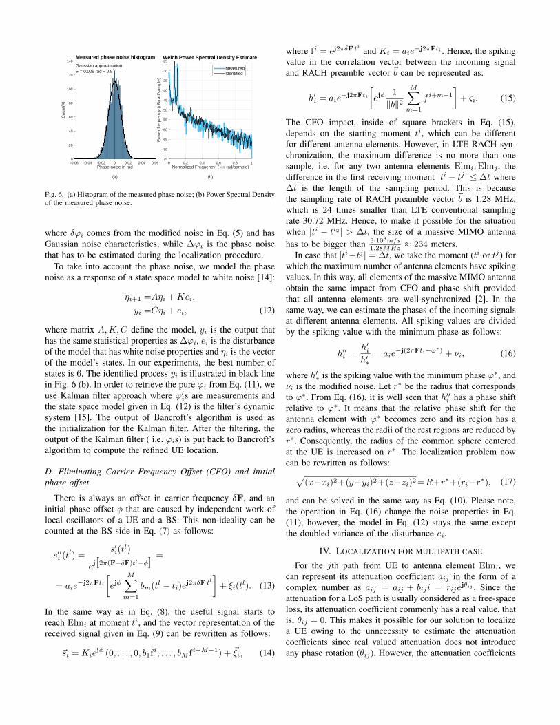
B. LoS localization during RACH synchronizationBecause of the use of SWP, each phase shift ϕi corresponds
to a certain distance Ri = λ× ϕi2π . As shown in Fig. 5, for each
is no larger than a half of the wavelength �/2 where � = c/F[12]. This guarantee that the difference in phase changesof the received signals between two neighboring antennaelements is no larger than ⇡ since the time for covering ahalf of the wavelength multiplied to the frequency in radiansis �
2c ⇥ 2⇡F = ⇡. Consequently, for any two neighboringantenna elements, the signal with the smallest phase can bealways found except in the situation where the difference isequal to ⇡. This case is not considered because the signalsare in fact transmitted exactly from the direction alongsidethe neighboring elements. In practice, such the situation isvery unlikely since a BS maintains a particular area, whichcancels situations with phase shift in ⇡ radians. Consequently,for any two neighboring antenna elements, the signal withsmaller phase can be always found based on the followingtwo rules:
• if |'i+1�'i| < ⇡, the smaller one remains to be smallerthan the bigger one;
• if |'i+1�'i| > ⇡, the smaller one becomes bigger sincethe difference between them cannot be bigger than ⇡, and2⇡ should be added to the smaller phase.
UE
BS'i+1 = 10⇡6
Im
Re
'i = ⇡6
�
�
ElmiElmi�1 Elmi+1
(a) (b)
�i+1
�i+211.1⇡6
�i�1
11⇡6
11.4⇡6
0.1⇡6
�i
Fig. 3. The phase rotation according to antenna elements.
As illustrated in Fig. 3(a), 'i = ⇡6 and 'i+1 = 10⇡
6 . Since|'i+1�'i| > ⇡, the actual difference should be 2⇡+ ⇡
6 � 10⇡6 ,
i.e. the difference represented by the arrrow with solid lineinstead of the one with the dashed line. Hence, 'i > 'i+1.
To compute the actual phase for the signal received at eachantenna element, we need to find the minimum phase for thesignals received at all antenna elements, which can be doneby performing pairwise comparison between neighbouringantenna elements based on the above two rules. Suppose thesignal received at antenna element Elmi has the minimumphase 'i. For each neighbour of Elmi denoted by Elmj , if|'j�'i| > ⇡, 'j = 'j+2⇡; otherwise 'j remains unchanged.We repeat the same operation for the neighbours of Elmj andso on until all 'is have been corrected. As illustrated in Fig.3(b), the minimum phase is 'i = 11⇡
6 . Since |'i+1�'i| < ⇡,'i+1 remains unchanged. But for 'i+2, |'i+2 � 'i+1| > ⇡.Hence, 'i+2 = 0.1⇡
6 +2⇡ = 12.1⇡6 . In such a way the ambiguity
caused by unknown quotient is eliminated.
B. LoS localization during RACH synchronizationBecause of the use of SWP, each phase shift 'i corresponds
to a certain distance Ri = �⇥ 'i
2⇡ .
2⇡N�
'1
'2
'N
Im
Re
Re
Re
UE(x, y, z)
BS
Elm1
Elm2
ElmN
RN
R2
R1
'1
'2
'N
Fig. 4. The phase rotation alongside the antenna array.
As shown in Fig. 4, for each antenna element Elmi, we drawa sphere centered at Elmi with radius of Ri. We further drawa sphere centred at the UE with radius of R = 2⇡N� so thatthis sphere is tangent to each sphere centred at Elmi wherei 2 [1, N ]. It can be seen that the LoS distance from the UE toantenna element Elmi can be rewritten by di = R + Ri, i =1, . . . , N . By representing di with the coordinates of the UE(x, y, z) and Elmi (xi, yi, zi), we have
p(x � xi)2 + (y � yi)2 + (z � zi)2 = R + Ri. (11)
To localize the UE, the BS needs to jointly estimate the UE’scoordinates and the common parameter N�. Since the numberof unknown parameters is four (x, y, z, R), the coordinates ofthe UE can be calculated if there are no less than 4 antennaelements, which is not a problem for BS with Massive MIMO[2], [?]. Once the BS has enough antenna elements, the aboveformulated localisation problem transforms to the classicalGNSS positioning problem that can be solved using Bancroft’salgorithm, which has a closed form solution [15].
C. Localization in the presence of carrier frequency offsetWhile the elements in one antenna array can be accurately
synchronised as they share the same oscillator, the UEsand BSs have independent local oscillators, and cannot beideally synchronized. Consequently, there are always a CarrierFrequency Offset (CFO) �F, and a phase offset � caused bydifferent starting moments of the oscillators. This non-idealitycan be counted at the BS side in Eq. (8) as follows:
s00i (tl) =s0i(t
l)
ej⇥2⇡(F��F)tl��
⇤ =
= aie�j2⇡Fti
ej�
MX
m=1
bm(tl � ti)ej2⇡�F tl
�+ ⇠i(t
l). (12)
In the same way as in (9), the useful signal starts to reach Elmi
at moment ti, and the vector representation of the receivedsignal given in Eq. (10) can be rewritten as follows:
~si = Kiej� (0, . . . , 0, b1f
i, . . . , bM fi+M�1) + ~⇠i, (13)
Fig. 3. The phase rotation according to antenna elements.
As illustrated in Fig. 3(a), 'i = ⇡6 and 'i+1 = 10⇡
6 . Since|'i+1�'i| > ⇡, the actual difference should be 2⇡+ ⇡
6 � 10⇡6 ,
i.e. the difference represented by the arrrow with solid lineinstead of the one with the dashed line. Hence, 'i > 'i+1.
To compute the actual phase for the signal received at eachantenna element, we need to find the minimum phase for thesignals received at all antenna elements, which can be doneby performing pairwise comparison between neighbouringantenna elements based on the above two rules. Suppose thesignal received at antenna element Elmi has the minimumphase 'i. For each neighbour of Elmi denoted by Elmj , if|'j�'i| > ⇡, 'j = 'j+2⇡; otherwise 'j remains unchanged.We repeat the same operation for the neighbours of Elmj andso on until all 'is have been corrected. As illustrated in Fig.3(b), the minimum phase is 'i = 11⇡
6 . Since |'i+1�'i| < ⇡,'i+1 remains unchanged. But for 'i+2, |'i+2 � 'i+1| > ⇡.Hence, 'i+2 = 0.1⇡
6 +2⇡ = 12.1⇡6 . In such a way the ambiguity
caused by unknown quotient is eliminated.
B. LoS localization during RACH synchronization
Because of the use of SWP, each phase shift 'i correspondsto a certain distance Ri = �⇥ 'i
2⇡ .
2⇡N�
'1
'2
'N
Im
Re
Re
Re
UE(x, y, z)
BS
Elm1
Elm2
ElmN
RN
R2
R1
'1
'2
'N
Fig. 4. The phase rotation alongside the antenna array.
As shown in Fig. 4, for each antenna element Elmi, we drawa sphere centered at Elmi with radius of Ri. We further drawa sphere centred at the UE with radius of R = 2⇡N� so thatthis sphere is tangent to each sphere centred at Elmi wherei 2 [1, N ]. It can be seen that the LoS distance from the UE toantenna element Elmi can be rewritten by di = R + Ri, i =1, . . . , N . By representing di with the coordinates of the UE(x, y, z) and Elmi (xi, yi, zi), we have
p(x � xi)2 + (y � yi)2 + (z � zi)2 = R + Ri. (11)
To localize the UE, the BS needs to jointly estimate the UE’scoordinates and the common parameter N�. Since the numberof unknown parameters is four (x, y, z, R), the coordinates ofthe UE can be calculated if there are no less than 4 antennaelements, which is not a problem for BS with Massive MIMO[2], [?]. Once the BS has enough antenna elements, the aboveformulated localisation problem transforms to the classicalGNSS positioning problem that can be solved using Bancroft’salgorithm, which has a closed form solution [15].
C. Localization in the presence of carrier frequency offset
While the elements in one antenna array can be accuratelysynchronised as they share the same oscillator, the UEsand BSs have independent local oscillators, and cannot beideally synchronized. Consequently, there are always a CarrierFrequency Offset (CFO) �F, and a phase offset � caused bydifferent starting moments of the oscillators. This non-idealitycan be counted at the BS side in Eq. (8) as follows:
s00i (tl) =s0i(t
l)
ej⇥2⇡(F��F)tl��
⇤ =
= aie�j2⇡Fti
ej�
MX
m=1
bm(tl � ti)ej2⇡�F tl
�+ ⇠i(t
l). (12)
In the same way as in (9), the useful signal starts to reach Elmi
at moment ti, and the vector representation of the receivedsignal given in Eq. (10) can be rewritten as follows:
~si = Kiej� (0, . . . , 0, b1f
i, . . . , bM fi+M�1) + ~⇠i, (13)
where fi = ej2⇡�F ti
and Ki = aie�j2⇡Fti . Hence, the spiking
value in the correlation vector between the incoming signal
Fig. 5. Phase shift at antenna elements alongside the antenna array.
antenna element Elmi, we draw a sphere centered at Elmi withradius of Ri. We further draw a sphere centred at the UE withradius of R = 2πNλ so that this sphere is tangent to eachsphere centred at Elmi where i ∈ [1, N ]. It can be seen thatthe LoS distance from the UE to antenna element Elmi can berewritten by di = R + Ri, i = 1, . . . , N . By representing diwith the coordinates of the UE (x, y, z) and Elmi (xi, yi, zi),we have
√(x− xi)2 + (y − yi)2 + (z − zi)2 = R+Ri. (10)
To localize the User Equipment (UE), the BS needs to jointlyestimate the UE’s coordinates and the common parameter Nλ.Since the number of unknown parameters is four (x, y, z, R),the coordinates of the UE can be calculated if there are noless than 4 antenna elements, which is not a problem forBS with Massive MIMO [2], [4]. Once the BS has enoughantenna elements, the above formulated localization problemtransforms to the classical GNSS positioning problem that canbe solved using the Bancroft’s algorithm, which has a closed-form solution [13].
C. Combating with phase noise
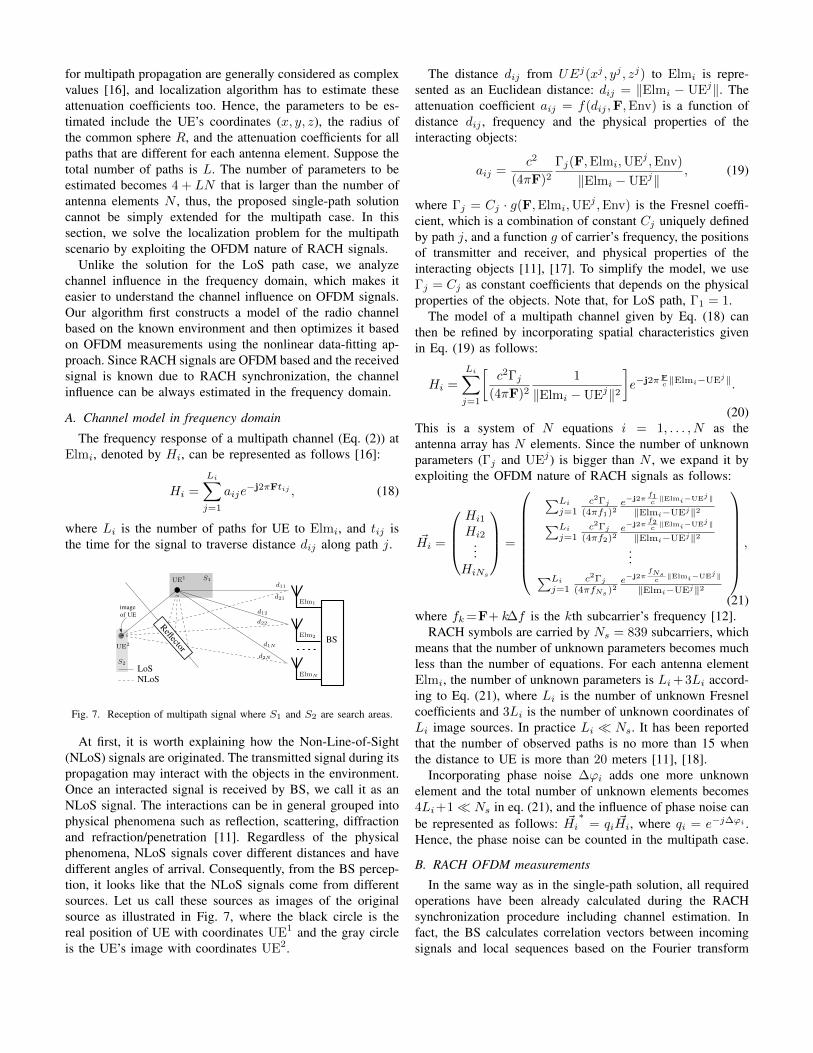
To understand how big is the phase noise between antennaelements in massive MIMO, we conduct experiments with twoEttus USRPs N210 synchronized via a NI OctoClock-G. OneUSRP periodically sends RACH signals to the other USRPthat calculates correlation between the incoming and localsignals and measures the phase of a correlation spike as inEq. (6). The testbed is operating with carrier frequency of 2.6GHz and sampling rate of 5.12 MS/s. To minimize wirelesschannel effects and guarantee a constant distance between thetransmitter and receiver, we connect the two antenna ports witha 1-meter long SMA-SMA cable. We run around 2900 roundsto measure the phase shifts.
As can be seen from Fig. 6(a), the phase deviations are toosmall to have a big impact on phase sorting. However, it cannot be ignored for the estimation of phase shift which has a bigimpact on localization accuracy. Fig. 6(b) shows the spectraldensity of the phase noise process. It can be seen that there area number of significant spikes. In the presence of such phasenoise, the estimated phase after sorting can be represented asfollows:
ϕ′i = ϕi + ∆ϕi + δϕi, (11)
0 0.2 0.4 0.6 0.8 1Normalized Frequency ( rad/sample)
(b)
-75
-70
-65
-60
-55
-50
-45
-40
-35
-30
-25
Pow
er/fr
eque
ncy
(dB
/rad
/sam
ple)
Welch Power Spectral Density Estimate
MeasuredIdentified
-0.06 -0.04 -0.02 0 0.02 0.04 0.06Phase noise in rad
(a)
0
20
40
60
80
100
120
140C
ount
(#)
Measured phase noise histogram
Gaussian approximation = 0.009 rad ~ 0.5°
Fig. 6. (a) Histogram of the measured phase noise; (b) Power Spectral Densityof the measured phase noise.
where δϕi comes from the modified noise in Eq. (5) and hasGaussian noise characteristics, while ∆ϕi is the phase noisethat has to be estimated during the localization procedure.
To take into account the phase noise, we model the phasenoise as a response of a state space model to white noise [14]:
ηi+1 =Aηi +Kei,
yi =Cηi + ei, (12)
where matrix A,K,C define the model, yi is the output thathas the same statistical properties as ∆ϕi, ei is the disturbanceof the model that has white noise properties and ηi is the vectorof the model’s states. In our experiments, the best number ofstates is 6. The identified process yi is illustrated in black linein Fig. 6 (b). In order to retrieve the pure ϕi from Eq. (11), weuse Kalman filter approach where ϕ′is are measurements andthe state space model given in Eq. (12) is the filter’s dynamicsystem [15]. The output of Bancroft’s algorithm is used asthe initialization for the Kalman filter. After the filtering, theoutput of the Kalman filter ( i.e. ϕis) is put back to Bancroft’salgorithm to compute the refined UE location.
D. Eliminating Carrier Frequency Offset (CFO) and initialphase offset
There is always an offset in carrier frequency δF, and aninitial phase offset φ that are caused by independent work oflocal oscillators of a UE and a BS. This non-ideality can becounted at the BS side in Eq. (7) as follows:
s′′i (tl) =s′i(t
l)
ej[2π(F−δF)tl−φ
] =
= aie−j2πFti
[ejφ
M∑
m=1
bm(tl − ti)ej2πδF tl
]+ ξi(t
l). (13)
In the same way as in Eq. (8), the useful signal starts toreach Elmi at moment ti, and the vector representation of thereceived signal given in Eq. (9) can be rewritten as follows:
~si = Kiejφ (0, . . . , 0, b1fi, . . . , bM fi+M−1) + ~ξi, (14)
where fi = ej2πδF ti
and Ki = aie−j2πFti . Hence, the spiking
value in the correlation vector between the incoming signaland RACH preamble vector ~b can be represented as:
h′i = aie−j2πFti
[ejφ
1
‖b‖2M∑
m=1
f i+m−1
]+ ςi. (15)
The CFO impact, inside of square brackets in Eq. (15),depends on the starting moment ti, which can be differentfor different antenna elements. However, in LTE RACH syn-chronization, the maximum difference is no more than onesample, i.e. for any two antenna elements Elmi,Elmj , thedifference in the first receiving moment |ti − tj | ≤ ∆t where∆t is the length of the sampling period. This is becausethe sampling rate of RACH preamble vector ~b is 1.28 MHz,which is 24 times smaller than LTE conventional samplingrate 30.72 MHz. Hence, to make it possible for the situationwhen |ti − ti2 | > ∆t, the size of a massive MIMO antennahas to be bigger than 3·108m/s
1.28MHz ≈ 234 meters.In case that |ti−tj | = ∆t, we take the moment (ti or tj) for
which the maximum number of antenna elements have spikingvalues. In this way, all elements of the massive MIMO antennaobtain the same impact from CFO and phase shift providedthat all antenna elements are well-synchronized [2]. In thesame way, we can estimate the phases of the incoming signalsat different antenna elements. All spiking values are dividedby the spiking value with the minimum phase as follows:
h′′i =h′ih′∗
= aie−j(2πFti−ϕ∗) + νi, (16)
where h′∗ is the spiking value with the minimum phase ϕ∗, andνi is the modified noise. Let r∗ be the radius that correspondsto ϕ∗. From Eq. (16), it is well seen that h′′i has a phase shiftrelative to ϕ∗. It means that the relative phase shift for theantenna element with ϕ∗ becomes zero and its region has azero radius, whereas the radii of the rest regions are reduced byr∗. Consequently, the radius of the common sphere centeredat the UE is increased on r∗. The localization problem nowcan be rewritten as follows:√
(x−xi)2+(y−yi)2+(z−zi)2 =R+r∗+(ri−r∗), (17)
and can be solved in the same way as Eq. (10). Please note,the operation in Eq. (16) change the noise properties in Eq.(11), however, the model in Eq. (12) stays the same exceptthe doubled variance of the disturbance ei.
IV. LOCALIZATION FOR MULTIPATH CASE
For the jth path from UE to antenna element Elmi, wecan represent its attenuation coefficient aij in the form of acomplex number as aij = aij + biji = rije
jθij . Since theattenuation for a LoS path is usually considered as a free-spaceloss, its attenuation coefficient commonly has a real value, thatis, θij = 0. This makes it possible for our solution to localizea UE owing to the unnecessity to estimate the attenuationcoefficients since real valued attenuation does not introduceany phase rotation (θij). However, the attenuation coefficients
for multipath propagation are generally considered as complexvalues [16], and localization algorithm has to estimate theseattenuation coefficients too. Hence, the parameters to be es-timated include the UE’s coordinates (x, y, z), the radius ofthe common sphere R, and the attenuation coefficients for allpaths that are different for each antenna element. Suppose thetotal number of paths is L. The number of parameters to beestimated becomes 4 + LN that is larger than the number ofantenna elements N , thus, the proposed single-path solutioncannot be simply extended for the multipath case. In thissection, we solve the localization problem for the multipathscenario by exploiting the OFDM nature of RACH signals.
Unlike the solution for the LoS path case, we analyzechannel influence in the frequency domain, which makes iteasier to understand the channel influence on OFDM signals.Our algorithm first constructs a model of the radio channelbased on the known environment and then optimizes it basedon OFDM measurements using the nonlinear data-fitting ap-proach. Since RACH signals are OFDM based and the receivedsignal is known due to RACH synchronization, the channelinfluence can be always estimated in the frequency domain.
A. Channel model in frequency domain
The frequency response of a multipath channel (Eq. (2)) atElmi, denoted by Hi, can be represented as follows [16]:
Hi =
Li∑
j=1
aije−j2πFtij , (18)
where Li is the number of paths for UE to Elmi, and tij isthe time for the signal to traverse distance dij along path j.
The CFO impact, inside of square brackets in Eq. (14),depends on the starting moment ti, which can be different fordifferent antenna elements. However, in Long Term Evolution(LTE) RACH synchronization, the maximum difference is nomore than one sample, i.e. for any two antenna elementsElmi, Elmj , the difference in the first receiving moment|ti � tj | �t where �t is the length of a sampling period.This is because the sampling rate of RACH preamble vector ~bis 1.28 MHz, which is 24 times smaller than LTE conventionalsampling rate 30.72 MHz. Hence, to make it possible for thesituation when |ti � ti2 | > �t, the size of a massive MIMOantenna has to be bigger than 3·108m/s
1.28MHz ⇡ 234 meters.In case that |ti � tj | = �t, we take that the moment (ti or
tj) for which the maximum number of antenna elements havespiking values. In this way all elements of the massive MIMOantenna obtain the same impact from CFO and phase shiftprovided that all antenna elements are well synchronized [?].In the same way we can estimate the phases of the incomingsignals at different antenna elements. All spiking values aredivided by the spiking value with the minimum phase asfollows:
h00i =
h0i
h0⇤= aie
�j(2⇡Fti�'⇤) + ⌫i, (15)
where h0⇤ is the spiking value with the minimum phase '⇤,
and ⌫i is the modified noise. Let r⇤ the radius that correspondsto '⇤. From Eq. (15), it is well seen that h00
i has a phase shiftrelative to '⇤. It means that the relative phase shift for theantenna element with '⇤ becomes zero and its region has azero radius, whereas the radii of the rest regions are reducedby r⇤. Consequently, the radius of the common sphere centredat the UE is increased on r⇤. The localization problem nowcan be rewritten as follows:p
(x � xi)2 + (y � yi)2 + (z � zi)2 =
= R + r⇤ + (ri � r⇤),(16)
and can be solved in the same way as Eq. (11).
VI. LOCALIZATION FOR MULTIPATH PATH CASE
For the jth path from UE to antenna element Elmk, wecan represent its attenuation coefficient akj in the form of acomplex number as akj = akj + bkji = rei✓kj . Since theattenuation for a LoS path is usually considered as free-spaceloss, its attenuation coefficient commonly has a real value, thatis, ✓kj = 0. This makes it possible for our solution to localizean UE owing to the unnecessity to estimate the attenuationcoefficients since real valued attenuation does not introduceany phase rotation (✓kj). However, the attenuation coefficientsfor multipath propagation are generally considered as complexvalues [9], and localization algorithm has to estimate theseattenuation coefficients too. Hence, the parameters to be es-timated include the UE’s coordinates (x, y, z), the radius ofthe common sphere R, and the attenuation coefficients forall paths. Suppose the total number of paths is L. Since thenumber of parameters to be estimated is 4 + L that is muchlarger than the number of antenna elements, the proposedsolution for LoS path case cannot be simply extended for
multipath case. In this section, we solve the UE localizationproblem for the multipath propagation scenario by exploitingthe OFDM nature of RACH signals.
Unlike the solution for the LoS path case, we analyzechannel influence in the frequency domain, which makes iteasier to understand the channel influence on OFDM signals.Our algorithm first constructs a model of the radio channelbased on the known environment, and then optimizes it basedon OFDM measurements using the nonlinear data-fitting ap-proach. Since RACH signals are OFDM based and the receivedsignal is known due to RACH synchronization, the channelinfluence can be always estimated in the frequency domain.
A. Channel model in frequency domainThe frequency response of a multipath channel (Eq. (3)) at
Elmi, denoted by Hi, can be represented as follows [9]:
Hi =
LiX
j=1
aije�j2⇡Ftij , (17)
where Li is the number of paths for UE to Elmi, and tij isthe time for the signal to traverse distance dij along path j.
S1
S2
UE1
BS
Elm1
Elm2
ElmN
Reflector
LoSNLoS
UE2
imageof UE
d11
d12
d1N
d21
d22
d2N
Fig. 5. Reception of multipath signal. The areas of search S1 and S2.
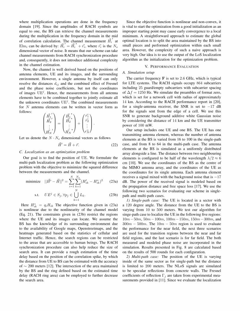
At first, it is worth explaining how the Non-Line-of-Sight(NLoS) signals are originated. The transmitted signal during itspropagation may interact with the objects in the environment.Once an interacted signal is received by BS, we call it as aNLoS signal. The interactions can be in general grouped intophysical phenomena such as reflection, scattering, diffractionand refraction/penetration [13]. Regardless the physical phe-nomena, NLoS signals cover different distances and have dif-ferent angles of arrival. Consequently, from the BS perception,it looks like that the NLoS signals come from different sources.Let us call these sources as images of the original source asillustrated in Fig. 5, where the black circle is the real positionof UE with coordinates UE1 and the gray circle is the UE’simage with coordinates UE2.
The distance dij from an image source UEj(xj , yj , zj)to Elmi can be represented as an Euclidean distance:dij = kElmi � UEjk. The attenuation coefficient aij =f(dij ,F, Env) is a function of distance dij , frequency andthe physical properties of the interacting objects:
aij =c2
(4⇡F)2�j(F, Elmi, UEj , Env)
kElmi � UEjk, (18)
Fig. 7. Reception of multipath signal where S1 and S2 are search areas.
At first, it is worth explaining how the Non-Line-of-Sight(NLoS) signals are originated. The transmitted signal during itspropagation may interact with the objects in the environment.Once an interacted signal is received by BS, we call it as anNLoS signal. The interactions can be in general grouped intophysical phenomena such as reflection, scattering, diffractionand refraction/penetration [11]. Regardless of the physicalphenomena, NLoS signals cover different distances and havedifferent angles of arrival. Consequently, from the BS percep-tion, it looks like that the NLoS signals come from differentsources. Let us call these sources as images of the originalsource as illustrated in Fig. 7, where the black circle is thereal position of UE with coordinates UE1 and the gray circleis the UE’s image with coordinates UE2.
The distance dij from UEj(xj , yj , zj) to Elmi is repre-sented as an Euclidean distance: dij = ‖Elmi − UEj‖. Theattenuation coefficient aij = f(dij ,F,Env) is a function ofdistance dij , frequency and the physical properties of theinteracting objects:
aij =c2
(4πF)2
Γj(F,Elmi,UEj ,Env)
‖Elmi −UEj‖, (19)
where Γj = Cj · g(F,Elmi,UEj ,Env) is the Fresnel coeffi-cient, which is a combination of constant Cj uniquely definedby path j, and a function g of carrier’s frequency, the positionsof transmitter and receiver, and physical properties of theinteracting objects [11], [17]. To simplify the model, we useΓj = Cj as constant coefficients that depends on the physicalproperties of the objects. Note that, for LoS path, Γ1 = 1.
The model of a multipath channel given by Eq. (18) canthen be refined by incorporating spatial characteristics givenin Eq. (19) as follows:
Hi =
Li∑
j=1
[c2Γj
(4πF)2
1
‖Elmi −UEj‖2]e−j2π
Fc ‖Elmi−UEj‖.
(20)This is a system of N equations i = 1, . . . , N as theantenna array has N elements. Since the number of unknownparameters (Γj and UEj) is bigger than N , we expand it byexploiting the OFDM nature of RACH signals as follows:
~Hi =
Hi1
Hi2...
HiNs
=
∑Lij=1
c2Γj(4πf1)2
e−j2πf1c‖Elmi−UEj‖
‖Elmi−UEj‖2∑Lij=1
c2Γj(4πf2)2
e−j2πf2c‖Elmi−UEj‖
‖Elmi−UEj‖2...
∑Lij=1
c2Γj(4πfNs )2
e−j2πfNsc‖Elmi−UEj‖
‖Elmi−UEj‖2
,
(21)where fk=F+ k∆f is the kth subcarrier’s frequency [12].
RACH symbols are carried by Ns = 839 subcarriers, whichmeans that the number of unknown parameters becomes muchless than the number of equations. For each antenna elementElmi, the number of unknown parameters is Li+3Li accord-ing to Eq. (21), where Li is the number of unknown Fresnelcoefficients and 3Li is the number of unknown coordinates ofLi image sources. In practice Li � Ns. It has been reportedthat the number of observed paths is no more than 15 whenthe distance to UE is more than 20 meters [11], [18].
Incorporating phase noise ∆ϕi adds one more unknownelement and the total number of unknown elements becomes4Li+1� Ns in eq. (21), and the influence of phase noise canbe represented as follows: ~Hi
∗= qi ~Hi, where qi = e−j∆ϕi .
Hence, the phase noise can be counted in the multipath case.
B. RACH OFDM measurements
In the same way as in the single-path solution, all requiredoperations have been already calculated during the RACHsynchronization procedure including channel estimation. Infact, the BS calculates correlation vectors between incomingsignals and local sequences based on the Fourier transform
where multiplication operations are done in the frequencydomain [19]. Since the amplitudes of RACH symbols areequal to one, the BS can retrieve the channel measurementsduring the multiplication in the frequency domain in the midof correlation calculation. The channel measurement ~Hi
′at
Elmi can be derived by: ~Hi′
= ~Hi∗
+ ~ri, where ~ri is the Nsdimensional vector of noise. It means that our scheme can takechannel measurements from RACH synchronization procedureand, consequently, it does not introduce additional complexityin the channel estimation.
Now, the channel is well derived based on the positions ofantenna elements, UE and its images, and the surroundingenvironment. However, a single antenna by itself can onlyresolve the distances dij and the combined effect of Fresneland the phase noise coefficients, but not the coordinatesof images UEj . Hence, the measurements from all antennaelements have to be combined together to jointly estimate allthe unknown coordinates UEj . The combined measurementsfor N antenna elements can be written in vector form asfollows:
~H1′
~H2′
...~HN′
=
~H1∗
~H2∗
...~HN∗
+
~r1
~r2...~rN
.
Let us denote the N ·Ns dimensional vectors as follows
~H ′ = ~H + ~r. (22)
C. Localization as an optimization problem
Our goal is to find the position of UE. We formulate themulti-path localization problem as the following optimizationproblem with the objective to minimize the squared differencebetween the measurements and the channel.
minimize || ~H ′ − ~H||2 =
N∑
i=1
Ns∑
k=1
(H ′ik −H∗ik)2 (23a)
s.t. UEj ∈ Sj ,∀pj ∈N⋃
k=1
Lk. (23b)
Here H∗ik = qiHik The objective function given in (23a)is nonlinear due to the nonlinearity of the channel model(Eq. 21). The constraints given in (23b) restrict the regionswhere the UE and its images can locate. We assume theBS has the knowledge of its surrounding environment dueto the availability of Google maps, Openstreetmaps, and theheatmaps generated based on the statistics of cellular andInternet traffic. Hence, the search regions can be restrictedto the areas that are accessible to human beings. The RACHsynchronization procedure can also help reduce the size ofsearch area. It can provide a rough estimation of the timedelay based on the position of the correlation spike, by whichthe distance from UE to BS can be estimated with the accuracyof ∼ 200 meters [12]. The intersection of the area maintainedby the BS and the ring defined based on the estimated timedelay (RACH ring area) can be employed to further decreasethe search area.
Since the objective function is nonlinear and non-convex, itis vital to start the optimization from a good initialization as animproper starting point may cause early convergence to a localminimum. A straightforward approach to estimate the globaloptimal location is to split the area maintained by the BS intosmall pieces and performed optimization within each smallarea. However, the complexity of such a naive approach isvery high. Our idea is to use the output of the LoS localizationalgorithm as the initialization for the optimization problem.
V. PERFORMANCE EVALUATION
A. Simulation setup
The carrier frequency F is set to 2.6 GHz, which is typicalfor LTE systems. The RACH signals occupy 864 subcarriersincluding 25 guard/empty subcarriers with subcarrier spacingof ∆f = 1250 Hz. We simulate the preambles of format zero,which is set for a network cell with radius of approximately14 km. According to the RACH performance report in [20],for a single-antenna receiver, the SNR is set to −17 dBfor the signals sent from the edge of a cell. We use thisSNR to generate background additive white Gaussian noiseby considering the distance of 14 km and the UE transmitterpower of 100 mW.
Our setup includes one UE and one BS. The UE has onetransmitting antenna element, whereas the number of antennaelements at the BS is varied from 16 to 100 in the single-pathcase, and from 8 to 64 in the multi-path case. The antennaelements at the BS is simulated as a uniformly distributedarray alongside a line. The distance between two neighbouringelements is configured to be half of the wavelength λ/2 ≈ 6cm [10]. We use the coordinates of the BS as the centre ofthe MIMO antenna array, and the coordinates of the UE asthe coordinates for its single antenna. Each antenna elementreceives a signal mixed with the background noise that is −17dB. The power of the received signal is modeled based onthe propagation distance and free space loss [17]. We use thefollowing two scenarios for evaluating our scheme in single-path and multi-path cases.
1) Single-path case: The UE is located in a sector witha 120 degree angle. The distance from the UE to the BS isvarying from 10 to 500 meters. We test our algorithm forsinge-path case to localize the UE in the following five regions:10m−50m, 50m−100m, 100m−150m, 150m−300m, and300m − 500m. The 10m − 50m region is used to evaluatethe performance for the near field, the next three scenariosare used for the transition regions between the near and farfield regions, and the last scenario is for far field. The bothmeasured and modeled phase noise are incorporated in thesimulation. Results presented in Fig. 8 are calculated basedon the results of 500 rounds for each configuration.
2) Multi-path case: The position of the UE is varyinginside of the same sector as for single-path but the distanceis limited to 200 meters. The NLoS signals are simulatedto be specular reflections from concrete walls. The Fresnelcoefficients of reflection Γj are taken from experimental mea-surements provided in [11]. Since we evaluate the localization
10-50m 50-100m 100-150m 150-300m 300-500m
Range of distances in meters
0.25m
0.5m
1m
1.5m
2m
2.5mR
MS
of l
ocat
ion
estim
atio
n er
ror
in m
eter
s16 Elm, BC16 Elm FK32 Elm, BC32 Elm FK64 Elm, BC64 Elm FK80 Elm, BC80 Elm FK100 Elm, BC100 Elm FK
(a)
10-50m 50-100m 100-150m 150-300m 300-500m
Range of distances in meters
10-3
10-2
10-1
RM
S o
f AoA
est
imat
ion
erro
r in
deg
rees 16 Elm, BC
16 Elm FK32 Elm, BC32 Elm FK64 Elm, BC64 Elm FK80 Elm, BC80 Elm FK100 Elm, BC100 Elm FK
(b)
(a)
#1040 0.4 0.8 1.2 1.6 2 2.4 2.8 3.2 3.5
Volts
#10-4
-6
-4
-2
0
2
4Measurements
Recording periods1 2 3 4 5 6 7 8 9
Sorte
d pha
ses
0
2
4
6
8
10
(b)
-0.1 0 0.1 0.2 0.3 0.4 0.5 0.6 0.7-0.2
-0.1
0
0.1
0.2
0.3
0.4
0.5
0.6
UE
(c)
Fig. 9. (a) Experiment Setup with USRP; (b) the estimated phases; (c) UE localization based on real measurements with an accuracy around 8 cm.
Number of antenna elements8 16 24 32 48 64
STD
of loc
ation
estim
ation
erro
r in m
eters
10-2
10-1
100
101
102
Single path algorithmMultipath algorithm
Fig. 8. Multipath: standard deviation of multipath localization error.
C. Hardware experiments with a single tone signal
We implemented the single path algorithm on a Ettus USRPN210 software radio platform emulating massive MIMO BSwith eight antenna elements. The transmitting and receivingUSRPs are synchronized using an external NI Octoclock-GCDA-2990. The transmitter repetitively transmits single tonesignal, and the receiver changes its position eight times toemulate an antenna array with eight elements as illustratedin Fig. 9(a). Once the receiver start to capture signals, thetransmitter start to record the transmitting signals. We performour experiment in an indoor setting with a heavy multipathoffice environment with moving objects and people.
Fig. 9(b) shows the the phase of the incoming signal atemulated antenna elements. It can be seen that the phasechanges consistently accordingly to the antenna element posi-tion, thereby justifying the feasibility of our solution. Fig. 9(c) illustrates the localisation results. It can be seen that theproposed single path algorithm well localizes the UE withan accuracy no larger than 8cm. Such a high accuracy isobtained because the LoS signal is still the dominating signaleven though the experiment was performed in a multi-pathpropagation environment.
VIII. CONCLUSION
In this paper, we propose two algorithms for LTE UElocalization during the RACH synchronization procedure. Thefirst algorithm is designed to localize UEs in the single paths
case using phase rotations of incoming signals, which can becaptured by the antenna elements of a massive MIMO at theBS. The second algorithm works in the multipath case, inwhich the multipath channel is modelled using the sphericalwave propagation assumption and linked to the propagationenvironment. We evaluate our schemes in bot simulations andexperiments, and results show that... The further developmentof the research lays in the extensive experimental validationof the proposed algorithms and enhancement of optimizationmethods.
REFERENCES
[1] K. Mahler, W. Keusgen, F. Tufvesson, T. Zemen, and G. Caire, “Propa-gation of multipath components at an urban intersection,” in 2015 IEEE82nd Vehicular Technology Conference (VTC2015-Fall), Sept 2015, pp.1–5.
[2] S. Zhang, P. Harris, A. Doufexi, A. Nix, and M. Beach, “Massive mimoreal-time channel measurements and theoretic tdd downlink throughputpredictions,” in 2016 IEEE 27th Annual International Symposium onPersonal, Indoor, and Mobile Radio Communications (PIMRC), Sept2016, pp. 1–6.
[3] D. Vasisht, S. Kumar, H. Rahul, and D. Katabi, “Eliminating channelfeedback in next-generation cellular networks,” in Proceedings ofthe 2016 Conference on ACM SIGCOMM 2016 Conference, ser.SIGCOMM ’16. New York, NY, USA: ACM, 2016, pp. 398–411.[Online]. Available: http://doi.acm.org/10.1145/2934872.2934895
[4] J. Flordelis, X. Gao, G. Dahman, F. Rusek, O. Edfors, and F. Tufves-son, “Spatial separation of closely-spaced users in measured massivemulti-user mimo channels,” in 2015 IEEE International Conference onCommunications (ICC), June 2015, pp. 1441–1446.
[5] E. Bjrnson, E. G. Larsson, and T. L. Marzetta, “Massive mimo: ten mythsand one critical question,” IEEE Communications Magazine, vol. 54,no. 2, pp. 114–123, February 2016.
[6] J. Vieira, F. Rusek, O. Edfors, S. Malkowsky, L. Liu, and F. Tufvesson,“Reciprocity calibration for massive mimo: Proposal, modeling, andvalidation,” IEEE Transactions on Wireless Communications, vol. 16,no. 5, pp. 3042–3056, May 2017.
[7] D. Vasisht, S. Kumar, and D. Katabi, “Sub-nanosecond time offlight on commercial wi-fi cards,” SIGCOMM Comput. Commun.Rev., vol. 45, no. 4, pp. 121–122, Aug. 2015. [Online]. Available:http://doi.acm.org/10.1145/2829988.2790043
[8] A. Fedorov, H. Zhang, and Y. Chen, “Geometry-based modeling andsimulation of 3d multipath propagation channel with realistic spatialcharacteristics,” in 2017 IEEE International Conference on Communi-cations (ICC), May 2017, pp. 1458–1464.
[9] D. Tse and P. Vishwanath, Fundamentals of Wireless Communication.Cambridge University Press, 2005.
[10] S. Sesia, I. Toufik, and M. Baker, LTE - The UMTS Long Term Evolution:From Theory to Practice. Chichester: John Wiley & Sons Ltd, 2011.
[11] D. Chu, “Polyphase codes with good periodic correlation properties(corresp.),” IEEE Transactions on Information Theory, vol. 18, no. 4,pp. 531–532, Jul 1972.
(c)
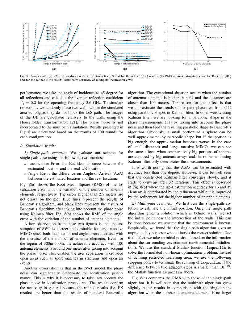
Fig. 8. Single-path: (a) RMS of localization error for Bancroft (BC) and for the refined (FK) results; (b) RMS of AoA estimation error for Bancroft (BC)and for the refined (FK) results. Multipath: (c) RMS of multipath localization error.
performance, we take the angle of incidence as 45 degree forall reflections and calculate the average reflection coefficientΓj = 0.3 for the operating frequency 2.6 GHz. To simulatereflections, we randomly place two walls within the simulatedarea as long as they do not block the LoS path. The imagesof the UE are calculated relatively to the walls using theHouseholder transformation [21]. The phase noise is notincorporated to the multipath simulation. Results presented inFig. 8 are calculated based on the results of 100 rounds foreach configuration.
B. Simulation results
1) Single-path scenario: We evaluate our scheme forsingle-path case using the following two metrics:• Localization Error: the Euclidean distance between the
estimated location and the real UE location;• Angle Error: the difference on Angle-of-Arrival (AoA)
between the estimated location and the real location.Fig. 8(a) shows the Root Mean Square (RMS) of the lo-calization error with the variation of the number of antennaelements, respectively. The errors higher than 2.5 meters arenot drawn on the plot. Blue lines represent the results ofBancroft’s algorithm, and black lines represent the results ofBancroft’s algorithm after taking into account the phase noiseusing Kalman filter. Fig. 8(b) shows the RMS of the angleerror with the variation of the number of antenna elements.
A key observation from these two figures is that the as-sumption of SWP is correct and desirable for large massiveMIMO since both localization and angle errors decrease withthe increase of the number of antenna elements. Even forthe region of 300m-500m, the achievable accuracy with 100antenna elements is around one meter after taking into accountthe phase noise. This enables the user separation in crowdedopen areas such as sport matches in stadiums and open airevents.
Another observation is that in the SWP model the phasenoise can significantly deteriorate the localization perfor-mance. This is why it is necessary to take into account thephase noise in localization procedures. The results confirmthe necessity in general because the refined results (i.e. FKresults) are better than the results of standard Bancroft’s
algorithm. The exceptional situation occurs when the numberof antenna elements is higher than 64 and the distances arecloser than 100 meters. The reason for this effect is thatwe approximate the trends of the pure phases ϕi from (11)using parabolic shapes in Kalman filter. In other words, usingKalman filter, we are looking for a parabolic shape in thephase measurements (11) by taking into account the phasenoise and then feed the resulting parabolic shape to Bancroft’salgorithm. Obviously, a small portion of a sphere can bewell approximated by parabolic shape but if the portion isbig enough, the approximation becomes worse. In the caseof small distances and large massive MIMO, we can seethe same effects when comparatively big portions of spheresare captured by big antenna arrays and the refinement usingKalman filter only deteriorates the measurements.
It is worth noting that the AoAs can be estimated withaccuracy less than one degree. However, it can be well seenthat the constructed Kalman filter converges slowly, and itstarts to converge after 32 iterations. This effect is observedin Fig. 8(b) where the AoA estimation accuracy for 16 and 32elements is deteriorated by the refinement while it is improvedby the refinement for the higher number of antenna elements.
2) Multi-path scenario: We first run the single-path so-lution to estimate the initial position. Once the single pathalgorithm gives a solution which is behind walls, we setthe initial point near the intersection of the walls. This canbe done because we assume that the environment is known.Empirically, we found that the single path algorithm gives anunpredictably big error when it looses the correct solution. Dueto this fact, we take an initial position based on the informationabout the surrounding environment (environmental initializa-tion). We use the standard Matlab function lsqnonlin tosolve the formulated non-linear optimization problem. Insteadof defining restricted searching area, we use the followingstopping policy to terminate the running of lsqnonlin: if thedifference between two adjacent steps is smaller than 10−19,the Matlab function lsqnonlin aborts.
Fig. 8(c) compares the RMS with those of the single-pathalgorithm. It is well seen that the multipath algorithm givesslightly better results in comparison with the single pathsalgorithm when the number of antenna elements is no larger
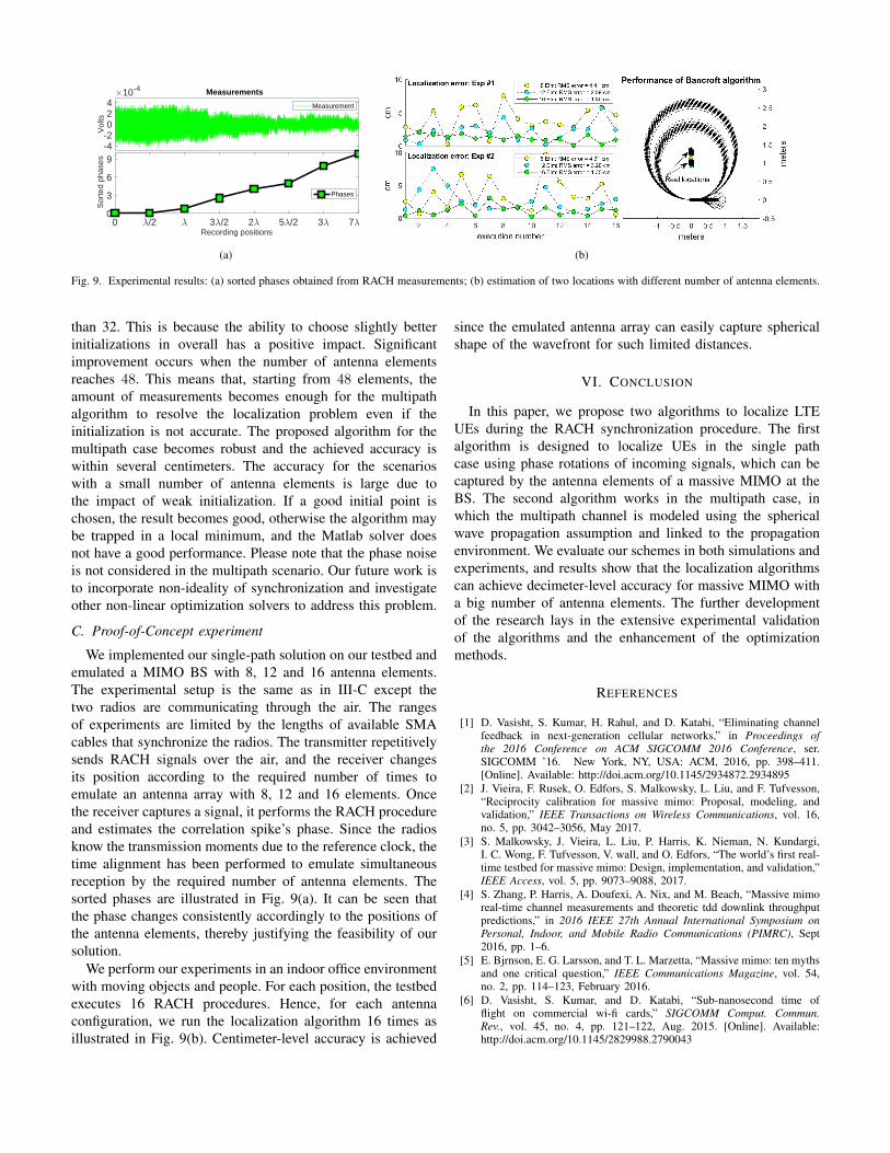
-4-2024
Vol
ts10-4 Measurements
Measurement
7 /235 /223 /2/20Recording positions
0
3
6
9
Sor
ted
phas
es
Phases
(a) (b)
Fig. 9. Experimental results: (a) sorted phases obtained from RACH measurements; (b) estimation of two locations with different number of antenna elements.
than 32. This is because the ability to choose slightly betterinitializations in overall has a positive impact. Significantimprovement occurs when the number of antenna elementsreaches 48. This means that, starting from 48 elements, theamount of measurements becomes enough for the multipathalgorithm to resolve the localization problem even if theinitialization is not accurate. The proposed algorithm for themultipath case becomes robust and the achieved accuracy iswithin several centimeters. The accuracy for the scenarioswith a small number of antenna elements is large due tothe impact of weak initialization. If a good initial point ischosen, the result becomes good, otherwise the algorithm maybe trapped in a local minimum, and the Matlab solver doesnot have a good performance. Please note that the phase noiseis not considered in the multipath scenario. Our future work isto incorporate non-ideality of synchronization and investigateother non-linear optimization solvers to address this problem.
C. Proof-of-Concept experiment
We implemented our single-path solution on our testbed andemulated a MIMO BS with 8, 12 and 16 antenna elements.The experimental setup is the same as in III-C except thetwo radios are communicating through the air. The rangesof experiments are limited by the lengths of available SMAcables that synchronize the radios. The transmitter repetitivelysends RACH signals over the air, and the receiver changesits position according to the required number of times toemulate an antenna array with 8, 12 and 16 elements. Oncethe receiver captures a signal, it performs the RACH procedureand estimates the correlation spike’s phase. Since the radiosknow the transmission moments due to the reference clock, thetime alignment has been performed to emulate simultaneousreception by the required number of antenna elements. Thesorted phases are illustrated in Fig. 9(a). It can be seen thatthe phase changes consistently accordingly to the positions ofthe antenna elements, thereby justifying the feasibility of oursolution.
We perform our experiments in an indoor office environmentwith moving objects and people. For each position, the testbedexecutes 16 RACH procedures. Hence, for each antennaconfiguration, we run the localization algorithm 16 times asillustrated in Fig. 9(b). Centimeter-level accuracy is achieved
since the emulated antenna array can easily capture sphericalshape of the wavefront for such limited distances.
VI. CONCLUSION
In this paper, we propose two algorithms to localize LTEUEs during the RACH synchronization procedure. The firstalgorithm is designed to localize UEs in the single pathcase using phase rotations of incoming signals, which can becaptured by the antenna elements of a massive MIMO at theBS. The second algorithm works in the multipath case, inwhich the multipath channel is modeled using the sphericalwave propagation assumption and linked to the propagationenvironment. We evaluate our schemes in both simulations andexperiments, and results show that the localization algorithmscan achieve decimeter-level accuracy for massive MIMO witha big number of antenna elements. The further developmentof the research lays in the extensive experimental validationof the algorithms and the enhancement of the optimizationmethods.
REFERENCES
[1] D. Vasisht, S. Kumar, H. Rahul, and D. Katabi, “Eliminating channelfeedback in next-generation cellular networks,” in Proceedings ofthe 2016 Conference on ACM SIGCOMM 2016 Conference, ser.SIGCOMM ’16. New York, NY, USA: ACM, 2016, pp. 398–411.[Online]. Available: http://doi.acm.org/10.1145/2934872.2934895
[2] J. Vieira, F. Rusek, O. Edfors, S. Malkowsky, L. Liu, and F. Tufvesson,“Reciprocity calibration for massive mimo: Proposal, modeling, andvalidation,” IEEE Transactions on Wireless Communications, vol. 16,no. 5, pp. 3042–3056, May 2017.
[3] S. Malkowsky, J. Vieira, L. Liu, P. Harris, K. Nieman, N. Kundargi,I. C. Wong, F. Tufvesson, V. wall, and O. Edfors, “The world’s first real-time testbed for massive mimo: Design, implementation, and validation,”IEEE Access, vol. 5, pp. 9073–9088, 2017.
[4] S. Zhang, P. Harris, A. Doufexi, A. Nix, and M. Beach, “Massive mimoreal-time channel measurements and theoretic tdd downlink throughputpredictions,” in 2016 IEEE 27th Annual International Symposium onPersonal, Indoor, and Mobile Radio Communications (PIMRC), Sept2016, pp. 1–6.
[5] E. Bjrnson, E. G. Larsson, and T. L. Marzetta, “Massive mimo: ten mythsand one critical question,” IEEE Communications Magazine, vol. 54,no. 2, pp. 114–123, February 2016.
[6] D. Vasisht, S. Kumar, and D. Katabi, “Sub-nanosecond time offlight on commercial wi-fi cards,” SIGCOMM Comput. Commun.Rev., vol. 45, no. 4, pp. 121–122, Aug. 2015. [Online]. Available:http://doi.acm.org/10.1145/2829988.2790043
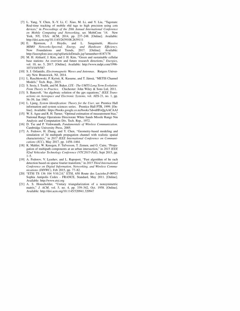
[7] L. Yang, Y. Chen, X.-Y. Li, C. Xiao, M. Li, and Y. Liu, “Tagoram:Real-time tracking of mobile rfid tags to high precision using cotsdevices,” in Proceedings of the 20th Annual International Conferenceon Mobile Computing and Networking, ser. MobiCom ’14. NewYork, NY, USA: ACM, 2014, pp. 237–248. [Online]. Available:http://doi.acm.org/10.1145/2639108.2639111
[8] E. Bjornson, J. Hoydis, and L. Sanguinetti, MassiveMIMO Networks:Spectral, Energy, and Hardware Efficiency.Now Foundations and Trends, 2017. [Online]. Available:http://ieeexplore.ieee.org/xpl/articleDetails.jsp?arnumber=8187178
[9] M. H. Alsharif, J. Kim, and J. H. Kim, “Green and sustainable cellularbase stations: An overview and future research directions,” Energies,vol. 10, no. 5, 2017. [Online]. Available: http://www.mdpi.com/1996-1073/10/5/587
[10] S. J. Orfanidis, Electromagnetic Waves and Antennas. Rutgers Univer-sity New Brunswick, NJ, 2014.
[11] L. Raschkowski, P. Kyosti, K. Kusume, and T. Jamsa, “METIS ChannelModels,” Tech. Rep., 2015.
[12] S. Sesia, I. Toufik, and M. Baker, LTE - The UMTS Long Term Evolution:From Theory to Practice. Chichester: John Wiley & Sons Ltd, 2011.
[13] S. Bancroft, “An algebraic solution of the gps equations,” IEEE Trans-actions on Aerospace and Electronic Systems, vol. AES-21, no. 1, pp.56–59, Jan 1985.
[14] L. Ljung, System Identification: Theory for the User, ser. Prentice Hallinformation and system sciences series. Prentice Hall PTR, 1999. [On-line]. Available: https://books.google.co.nz/books?id=nHFoQgAACAAJ
[15] W. S. Agee and R. H. Turner, “Optimal estimation of measurement bias,”National Range Operations Directorate White Sands Missile Range NmAnalysis and Computation Div, Tech. Rep., 1972.
[16] D. Tse and P. Vishwanath, Fundamentals of Wireless Communication.Cambridge University Press, 2005.
[17] A. Fedorov, H. Zhang, and Y. Chen, “Geometry-based modeling andsimulation of 3d multipath propagation channel with realistic spatialcharacteristics,” in 2017 IEEE International Conference on Communi-cations (ICC), May 2017, pp. 1458–1464.
[18] K. Mahler, W. Keusgen, F. Tufvesson, T. Zemen, and G. Caire, “Propa-gation of multipath components at an urban intersection,” in 2015 IEEE82nd Vehicular Technology Conference (VTC2015-Fall), Sept 2015, pp.1–5.
[19] A. Fedorov, V. Lyashev, and L. Rapoport, “Fast algorithm of lte rachdetection based on sparse fourier transform,” in 2015 Third InternationalConference on Digital Information, Networking, and Wireless Commu-nications (DINWC), Feb 2015, pp. 77–82.
[20] “ETSI TS 136 104 V10.2.0,” ETSI, 650 Route des Lucioles,F-06921Sophia Antipolis Cedex - FRANCE, Standard, May 2011. [Online].Available: http://www.etsi.org
[21] A. S. Householder, “Unitary triangularization of a nonsymmetricmatrix,” J. ACM, vol. 5, no. 4, pp. 339–342, Oct. 1958. [Online].Available: http://doi.acm.org/10.1145/320941.320947