electronics

Article

User-Driven Fine-Tuning for Beat Tracking

António S. Pinto 1,* , Sebastian Böck 2 , Jaime S. Cardoso 1 and Matthew E. P. Davies 3

�����������������

Citation: Pinto, A.S.; Böck, S.;

Cardoso, J.S.; Davies, M.E.P.

User-Driven Fine-Tuning for Beat

Tracking. Electronics 2021, 10, 1518.

https://doi.org/10.3390/

electronics10131518

Academic Editors: Alexander Lerch

and Peter Knees

Received: 25 May 2021

Accepted: 18 June 2021

Published: 23 June 2021

Publisher’s Note: MDPI stays neutral

with regard to jurisdictional claims in

published maps and institutional affil-

iations.

Copyright: © 2021 by the authors.

Licensee MDPI, Basel, Switzerland.

This article is an open access article

distributed under the terms and

conditions of the Creative Commons

Attribution (CC BY) license (https://

creativecommons.org/licenses/by/

4.0/).

1 INESC TEC, Centre for Telecommunications and Multimedia, 4200-465 Porto, Portugal;jaime.cardoso@inesctec.pt

2 enliteAI, 1000-1901 Vienna, Austria; s.boeck@enlite.ai3 Centre for Informatics and Systems, Department of Informatics Engineering, University of Coimbra,

3030-290 Coimbra, Portugal; mepdavies@dei.uc.pt* Correspondence: antonio.s.pinto@inesctec.pt

Abstract: The extraction of the beat from musical audio signals represents a foundational task in thefield of music information retrieval. While great advances in performance have been achieved duethe use of deep neural networks, significant shortcomings still remain. In particular, performanceis generally much lower on musical content that differs from that which is contained in existingannotated datasets used for neural network training, as well as in the presence of challenging musicalconditions such as rubato. In this paper, we positioned our approach to beat tracking from a real-worldperspective where an end-user targets very high accuracy on specific music pieces and for which thecurrent state of the art is not effective. To this end, we explored the use of targeted fine-tuning ofa state-of-the-art deep neural network based on a very limited temporal region of annotated beatlocations. We demonstrated the success of our approach via improved performance across existingannotated datasets and a new annotation-correction approach for evaluation. Furthermore, wehighlighted the ability of content-specific fine-tuning to learn both what is and what is not the beat inchallenging musical conditions.

Keywords: beat tracking; transfer learning; user adaptation

1. Introduction

A long-standing area of investigation in music information retrieval (MIR) is thecomputational rhythm analysis of musical audio signals. Within this broad research area,which incorporates many diverse facets of musical rhythm including onset detection [1],tempo estimation [2] and rhythm quantisation [3], sits the foundational task of musicalaudio beat tracking. The goal of beat tracking systems is commonly stated as inferringand then tracking a quasi-regular pulse so as to replicate the way a human listener mightsubconsciously tap their foot in time to a musical stimulus [4–6]. However, the pursuit ofcomputational beat tracking is not limited to emulating an aspect of human music percep-tion. Rather, it has found widespread use as an intermediate processing step within largerscale MIR problems by allowing the analysis of harmony [7] and long-term structure [8]in “musical time” thanks to beat-synchronous processing. In addition, the imposition of abeat grid on a musical signal can enable the extraction and understanding of expressiveperformance attributes such as microtiming [9]. Furthermore, within creative applica-tions of MIR technology, the accurate extraction of the beat is of critical importance forsynchronisation and thus plays a pivotal role in automatic DJ mixing between differentpieces of music [10], as well as the layering of music signals for mashup creation [11]. Inparticular for musicological and creative applications, the need for very high accuracy isparamount as the quality of the subsequent analysis and/or creative musical result willdepend strongly on the accuracy of the beat estimation.

From a technical perspective, computational approaches to musical audio beat tracking(as with many MIR tasks) have undergone a profound transformation due to the prevalence

Electronics 2021, 10, 1518. https://doi.org/10.3390/electronics10131518 https://www.mdpi.com/journal/electronics

Electronics 2021, 10, 1518 2 of 23

of deep neural networks. While numerous traditional approaches to beat tracking exist,it can be argued that they follow a largely similar set of processing steps: (i) the calculationof a time–frequency representation such as a short-time Fourier transform (STFT) from theaudio signal; (ii) the extraction of one or more mid-level representations from the STFT, e.g.,the use of complex spectral difference [12] or other so-called “onset detection functions” [13],whose local maxima are indicative of the temporal locations of note onsets; and (iii) thesimultaneous or sequential estimation of the periodicity and phase of the beats from thisonset detection function (or an extracted discrete sequence of onsets) with techniquessuch as autocorrelation [14], comb filtering [15], multi-agent systems [16,17] and dynamicprogramming [18]. The efficacy of these traditional approaches was demonstrated via theirevaluation on annotated datasets, many of which were small and not publicly available.

By contrast, more recent supervised deep learning approaches sharply diverge fromthis formulation in the sense that they start with, and explicitly depend on, access to largeamounts of annotated training data. The prototypical deep learning approach, perhapsbest typified by Böck and Schedl [19], formulates beat tracking as a sequential learningproblem of binary classification through time, where beat targets are rendered as impulsetrains. The goal of a beat-tracking deep neural network, typically by means of recurrentand/or convolutional architectures, is to learn to predict a beat activation function froman input representation (either the audio signal itself or a time–frequency transformation),which closely resembles the target impulse train. While in some cases, it can be sufficient toemploy thresholding and/or peak-picking to obtain a final output sequence of beats fromthis beat activation function, the de facto standard is to use a dynamic Bayesian network(DBN) [20] approximated by a hidden Markov model (HMM) [21] for inference, which isbetter able to contend with spurious peaks or the absence of reliable information. Given thisexplicit reliance on annotated training data, together with the well-known property ofneural networks to “overfit” to training data, great care must be taken when evaluatingthese systems to ensure that all test data remain unseen by the network in order to permitany meaningful insight into the generalisation capabilities.

Following this data-driven formulation, the state of the art in beat tracking has im-proved substantially over the last 10 years, with the most recent approaches using temporalconvolutional networks [22], achieving accuracy scores in excess of 90% on diverse anno-tated datasets comprised of rock, pop, dance and jazz musical excerpts [23–26]. Yet, in spiteof these advances, several challenges and open questions remain. Deep learning methodsare known to be highly data-sensitive [27]. The knowledge they acquire is directly linkedboth to the quality of the annotated data and the scope of musical material to which theyhave been exposed. In this sense, it is hard to predict the efficacy of a beat tracking systemwhen applied to “unfamiliar” (i.e., outside of the dataset) musical material; indeed, evenstate-of-the-art systems that perform very well on Western music have been shown to per-form poorly on non-Western music [9]. Likewise, given the arduous nature of the manualannotation of beat locations for the creation of annotated datasets, there is an implicit biastowards more straightforward musical material, e.g., with a roughly constant tempo, 4/4metre, and the presence of drums [28,29]. In this way, more challenging musical material,e.g., containing highly expressive tempo variation, non-percussive content, changing me-tres, etc., is under-represented, and its relative scarcity in annotated datasets may contributeto poorer performance. Furthermore, the great majority of annotated datasets comprisemusical excerpts of up to one minute in duration, meaning that the ability of these systemsto track entire musical pieces in a structurally consistent manner is largely unknown.

The scope and motivation for this paper were to move away from the notion oftargeting and then reporting high (mean) accuracy across existing annotated datasets andinstead to move towards the real-world use of beat tracking systems by end-users onspecific musical pieces. More specifically, we investigated what to do when even the stateof the art is not effective and very high accuracy is required, i.e., when the extraction of thebeat is used to drive higher level musicological analysis or creative musical repurposing.

Electronics 2021, 10, 1518 3 of 23

Faced with this situation, currently available paths of action include: (i) the end-user performing manual corrections to the beat output or even resorting to a completere-annotation by hand, which may be extremely time-consuming and labour-intensive;(ii) the use of some high-level parameterisation of the algorithm in terms of an expectedtempo range and initial phase [16,30]; or (iii) adapting some more abstract parametersthat could permit greater flexibility in tracking tempo variation [31]. While at first sightpromising, this high-level information may only help in a very limited way: if the musicalcontent is very expressive, then knowing some initial tempo might not be useful later onin the piece. Likewise, if the model is unable to make reliable predictions of the beat-likestructure given the presence of different signal properties (e.g., timbre), then this userprovided information may only be useful in very localised regions.

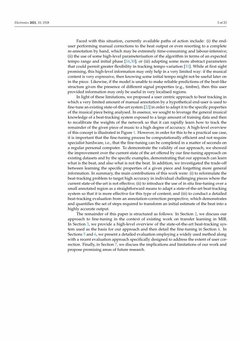
In light of these limitations, we proposed a user centric approach to beat tracking inwhich a very limited amount of manual annotation by a hypothetical end-user is used tofine-tune an existing state-of-the-art system [22] in order to adapt it to the specific propertiesof the musical piece being analysed. In essence, we sought to leverage the general musicalknowledge of a beat-tracking system exposed to a large amount of training data and thento recalibrate the weights of the network so that it can rapidly learn how to track theremainder of the given piece of music to a high degree of accuracy. A high-level overviewof this concept is illustrated in Figure 1. However, in order for this to be a practical use case,it is important that the fine-tuning process be computationally efficient and not requirespecialist hardware, i.e., that the fine-tuning can be completed in a matter of seconds ona regular personal computer. To demonstrate the validity of our approach, we showedthe improvement over the current state of the art offered by our fine-tuning approach onexisting datasets and by the specific examples, demonstrating that our approach can learnwhat is the beat, and also what is not the beat. In addition, we investigated the trade-offbetween learning the specific properties of a given piece and forgetting more generalinformation. In summary, the main contributions of this work were: (i) to reformulate thebeat-tracking problem to target high accuracy in individual challenging pieces where thecurrent state-of-the-art is not effective; (ii) to introduce the use of in situ fine-tuning over asmall annotated region as a straightforward means to adapt a state-of-the-art beat-trackingsystem so that it is more effective for this type of content; and (iii) to conduct a detailedbeat-tracking evaluation from an annotation-correction perspective, which demonstratesand quantifies the set of steps required to transform an initial estimate of the beat into ahighly accurate output.

The remainder of this paper is structured as follows: In Section 2, we discuss ourapproach to fine-tuning in the context of existing work on transfer learning in MIR.In Section 3, we provide a high-level overview of the state-of-the-art beat-tracking sys-tem used as the basis for our approach and then detail the fine-tuning in Section 4. InSections 5 and 6, we present a detailed evaluation employing a widely used method alongwith a recent evaluation approach specifically designed to address the extent of user cor-rection. Finally, in Section 7, we discuss the implications and limitations of our work andpropose promising areas of future research.

Electronics 2021, 10, 1518 4 of 23

pre-trainednetwork

prediction prediction

fine-tunednetwork

input audio with user beatsinput audio

0 5 10-0.05

0

0.05

0 5 10-0.05

0

0.05

0 5 10 0 5 100

0.5

0

0.5

time (s)time (s)

time (s)time (s)

Figure 1. Overview of our proposed approach. The left column shows an audio input passed througha deep neural network (for consistency with our approach, this is a temporal convolutional network),which produces a weak beat activation function and erroneous beat output. The right column showsthe same audio input, but here, a few beat annotations are provided as the means to fine-tune thenetwork—with the black arrows implying the modification of some of the weights of the network.This results in a much clearer beat activation function and an accurate beat-tracking output.

2. Low-Data Learning Strategies

Data scarcity represents a major bottleneck for machine learning in general, but particu-larly for deep learning. Within the musical audio domain, data curation is often hindered bythe laborious and expensive human annotation process, subjectivity and content availabil-ity limitations due to copyright issues, thus making the field of MIR an interesting use-casefor machine learning strategies to address low-data regimes [32]. Following success in theresearch domains of computer vision and natural language processing, a wide range ofapproaches have been proposed to overcome this limitation in the audio domain. In this pa-per, we focused on one such approach, transfer learning, through which knowledge gainedduring training in one type of problem is used to train another related task or domain [33].Leveraging previously acquired knowledge and avoiding a cold-start (i.e., training “fromscratch”), it can enable the development of accurate models in a cost-effective way.

Early approaches to transfer learning in MIR were based on the use of pretrainedmodels on large datasets for feature extraction and have been proposed for tasks such asgenre classification and auto-tagging [34], speech/music classification or music emotionprediction [35]. A different methodology is the use of pretrained weights as an initializationfor the parameters of the downstream model. This technique, known as fine-tuning, proposesthe subsequent retraining of certain parts of the network by defining which weights to“unfreeze” while retaining the existing knowledge in the “frozen” components. This pa-rameter transfer learning approach has been used for the adaptive generation of rhythmmicrotiming [36] and for beat tracking, as a way to transfer the knowledge of a networktrained on popular music into tracking beats in Greek folk music [37].

Another strategy for low-data regimes is known as few-shot learning, which aims atgeneralizing from only a few examples [38]. Both paradigms have been studied for mu-sic classification tasks [39]. Lately, the association between both approaches has becomewidespread, with transfer learning techniques being widely deployed in few-shot classi-

Electronics 2021, 10, 1518 5 of 23

fication, achieving high performance with a simplicity that has made fine-tuning the defacto baseline method for few-shot learning [40], in what is known as transductive transferlearning [33].

Within the context of musical audio beat tracking, we employed fine-tuning not forthe adaption to a new task per se, but rather to new content within the same task. In formalterms, this can be considered sequential inductive transfer learning. Our approach differsfrom that of Fiocchi et al. [37] since we targeted a kind of controlled overfitting to a specificpiece of music rather than a collection of musical excerpts in a given style. In this sense,our approach bears some high-level similarity to the use of “bespoke” networks for audiosource separation [41]. While the need to rely on some minimal annotation effort couldbe seen as an inefficiency in a processing pipeline, which, in many MIR contexts, is fullyautomatic [42], our approach may offer the means to address subjectivity in beat perceptionvia personalised analysis.

3. Baseline Beat-Tracking Approach

A key motivating factor and contribution of this work is to look beyond what ispossible with the current state of the art in beat tracking, and hence to explore fine-tuningas a means for content-specific adaptation. To this end, we restricted the scope of this workto an explicit extension of the most recent state-of-the-art approach [22], and thus used thisas a baseline on which to measure improvement.

The baseline approach uses multi-task learning for the simultaneous estimation ofbeat, downbeat and tempo. The core of the approach is a temporal convolutional network(TCN), which was first used for beat tracking only in [43], and then expanded to predictboth tempo and beat [44]. Compared to previous recurrent architectures for beat tracking(e.g., [45]), TCNs have the advantage that they retain the high parallelisation property ofconvolutional neural networks (CNNs), and therefore can be trained more efficiently overlarge training data [43]. With the long-term goal of integrating in situ fine-tuning within auser based workflow for a given piece of music, we considered this aspect of efficiency tobe particularly important, and this therefore formed a secondary motivation to extend theTCN-based approach.

To provide a high-level overview of this approach ahead of the discussion of fine-tuning, and to enable this paper to be largely self-contained, we now summarise themain aspects of the processing pipeline, network architecture and training procedure.For complete details, see [22].

Pre-processing: Given a mono audio input signal, sampled at 44.1 kHz, the input rep-resentation is a log magnitude spectrogram obtained with a Hann window of 46.4 ms(2048 samples) and a hop length of 10 ms. Subsequently, a logarithmic grouping of fre-quency bins with 12 bands per octave gives a total of 81 frequency bands from 30 Hz up to17 kHz.

Neural network: The neural network was comprised of two stages: a set of threeconvolutional and max pooling layers followed by a TCN block. The goal of the convolu-tional and max pooling layers was to learn a compact intermediate representation fromthe musical audio signal, which could then be passed to the TCN as the main sequencelearning model. The shapes of the three convolutional and max pooling layers were asfollows: (i) 3 × 3 followed by 1 × 3 max pooling; (ii) 1 × 10 followed by 1 × 3 max pooling;and (iii) 3 × 3 again with 1 × 3 max pooling. A dropout rate of 0.15 was used with theexponential linear unit (ELU) as the activation function.

This compact intermediate representation was then fed into a TCN block that operatednoncausally (i.e., with dilations spanning both forwards and backwards in time). The TCNblock was composed of two sets of geometrically spaced dilated convolutions over elevenlayers with one-dimensional filters of size five. The first of the dilations spanned therange of 20 up to 210 frames and the second at twice this rate. The feature maps of thetwo dilated convolutions were concatenated before spatial dropout (with a rate of 0.15)and the ELU as activation function. Finally, in order to keep the output dimensionality

Electronics 2021, 10, 1518 6 of 23

of the TCN layer consistent, these feature maps were combined with a 1 × 1 convolution.Within the multitask approach (and unlike the simultaneous estimation in [45]), the beatand downbeat targets were separate, each produced by a sigmoid on a fully connectedlayer. The tempo classification output was produced by a softmax layer. In total, twentyfilters were learned within this network, giving approximately 116 k weights. A graphicaloverview of the network is given in Figure 2.

Training: The network was trained on the following six reference datasets, whichtotalled more than 26 h of musical material: Ballroom [26,46], Beatles [24], Hainsworth [23,44],HJDB [45,47], Simac [48] and SMC [28]. In order to account for gaps in the distributionof the tempi of these datasets, a data augmentation strategy was adopted, by which thetraining data were enlarged by a factor of 10, by varying the overlap rate of the framesof the STFT (and hence the tempo) and by sampling from a normal distribution with the5% standard deviation around the annotated tempo and updating the beat, downbeatand tempo targets accordingly. Furthermore, to account for the high imbalance betweenpositive and negative examples (i.e., that frames labelled as beats occurred much less oftenthan nonbeat frames), the beat and downbeat targets were widened by ±2 frames andweighted by 0.5 and 0.25 as they diverged from the central beat frame.

Convolutional and Max Pooling Block

TCN Block

MaxPooling

k=1x3

Dropout

rate=0.15

Conv2D

k=1x10

MaxPooling

k=1x3

Dropout

rate=0.15

Conv2D

k=3x3(3,79,20) (3,26,20)

(3,17,20) (3,5,20)

Conv2D

k=3x3

MaxPooling

k=1x3

Dropout

rate=0.15

(1,3,20) (1,1,20)

Dilated Convolution1

k=5x1; dr1 Conv1D

k=1+

Conv1D

k=1

Residual

Spatial Dropoutrate=0.15

Dropout

rate=0.15

To next TCN layer

(1,1,1)

Input

Log-mag Spectrogram

(5,81,1)

Dilated Convolution2

k=5x1; dr2=2dr1

ELU

ELU

ELU

DenseSigmoid

Dropout

rate=0.15

Dense

(1,1,300)

Softmax

Global Avg. Pooling

ELU

Dropout

rate=0.15

Gaussian Noise

Output

Beat Activation

Output

Tempo

Dropout

rate=0.15(1,1,1)

DenseSigmoid

Output

Downbeat Activation

+

Skip Connections

(1,1,20)

(1,1,20) (1,1,20)

(1,1,40)

Figure 2. Overview diagram of the architecture of the baseline beat-tracking approach.

The training was conducted using eight-fold cross validation (6 folds for training,1 fold for validation, and 1 fold held-back for testing), with excerpts from each datasetuniformly distributed across the folds. A maximum of 200 training epochs per fold wereused with a learning rate of 0.002, which was halved after no improvement in the validationloss for 20 epochs, and early stopping was activated with no improvement after 30 epochs.

Electronics 2021, 10, 1518 7 of 23

The RAdam optimiser followed by lookahead optimization were used with a batch size of oneand gradient clipping at a norm of 0.5.

Postprocessing: To obtain the final output, the beat activation and downbeat activationswere combined and passed as the input to a dynamic Bayesian network approximated viaan HMM [45], which simultaneously decoded the beat times and labels corresponding tometrical position (i.e., where the all beats labelled 1 were downbeats). However, given onlythe beat activation function, it was possible to use the beat-only HMM for inference [21].

4. Fine-Tuning

Departing from the network architecture described above, we now turn our attentiontoward how we could adapt it to successfully analyse very challenging musical pieces.It is important to restate that our interest was specifically in musical content for which thecurrent state-of-the-art approach is not effective and for which high accuracy is desired bysome end-user. Within this scenario, it is straightforward to envisage that some form ofuser input could be beneficial to guide the estimation of the beat.

In a broad sense, our strategy was to take advantage of the transferability of featuresin neural networks [49], in effect to leverage the global knowledge about beat trackingfrom the baseline approach and the datasets upon which it has been trained, and torecalibrate it to fit the musical properties of a given new piece. By connecting this concept oftransferability with an end-user who actively participated in the analysis and a prototypicalbeat annotation workflow, we formulated the network adaption as a process of fine-tuningbased on a small temporal region of manually annotated beat positions. From the userperspective, this implies a small annotation effort to mark a few beats by hand, and thenusing this information as the basis for updating the weights of the baseline network suchthat the complete piece can be accurately analysed with minimal further user interaction.

Within this paper, our primary interest was to understand the viability of this ap-proach, rather than testing it in real-world conditions. To this end, we simulated the annotationeffort of the end-user by using ground truth annotations over a small temporal regionand examining how well the adapted network could track the remainder of the piece.From a technical perspective, we began with a pretrained model from the baseline ap-proach described in the previous section. Then, for a given musical excerpt (unseen to thepretrained model), we isolated a small temporal region (nominally near the start of theexcerpt), which we set to be 10 s in duration, and retrieved the corresponding ground truthbeat annotations. Together, these three components formed the basis of our fine-tuningapproach, as illustrated in Figure 1. In devising this approach, we focused on: (i) how toparameterise the fine-tuning; (ii) when to stop the fine-tuning; and (iii) how to cope withthe very limited amount of new information provided by the small temporal region.

Fine-tuning parameterisation: The first consideration in our fine-tuning approach wasto examine which layers of the baseline network to update. It is commonplace in transferlearning to freeze all but the last layers of the network [50]. However, in our context, oneimportant means for adapting the network resides in modelling how the beat is conveyedwithin the log magnitude spectrogram itself (i.e., unfamiliar musical timbres such as thehuman voice). To this end, we allowed all the layers of the network to be updated bythe fine-tuning process. Since our focus in this paper was restricted to beat tracking, wemasked the losses for the tempo and downbeat tasks. From a practical perspective, thisalso means that we did not require downbeat or tempo annotations across the 10 s temporalregion. Concerning the parameterisation of the fine-tuning, we followed common practicein transfer learning and reduced the learning rate, setting it to 0.0004 (i.e., one fifth of therate used in the baseline).

Stopping criteria: The next area was to address when to stop fine-tuning. In morestandard approaches for training deep neural networks, e.g., our baseline approach, cross-fold validation is used with the validation loss driving the adjustment of the learningrate and the execution of early stopping. In our approach, if we were to use the entire10 s region for training, then it would be difficult to exercise control over the extent of

Electronics 2021, 10, 1518 8 of 23

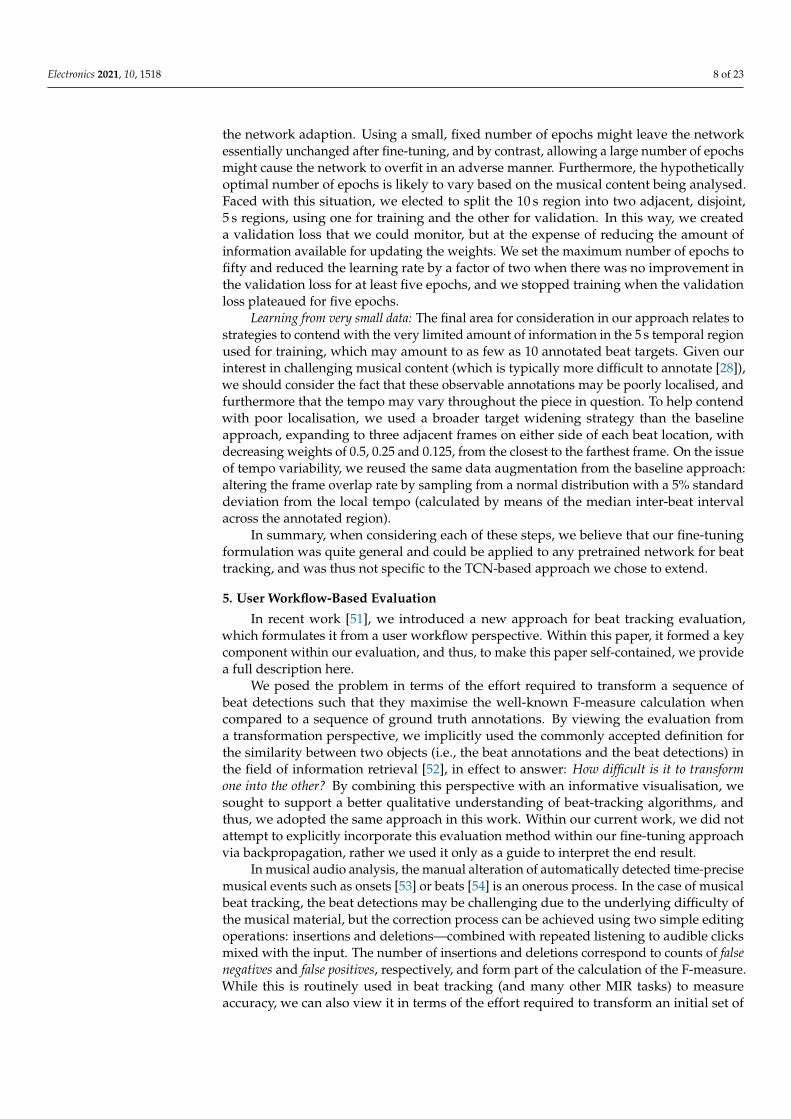
the network adaption. Using a small, fixed number of epochs might leave the networkessentially unchanged after fine-tuning, and by contrast, allowing a large number of epochsmight cause the network to overfit in an adverse manner. Furthermore, the hypotheticallyoptimal number of epochs is likely to vary based on the musical content being analysed.Faced with this situation, we elected to split the 10 s region into two adjacent, disjoint,5 s regions, using one for training and the other for validation. In this way, we createda validation loss that we could monitor, but at the expense of reducing the amount ofinformation available for updating the weights. We set the maximum number of epochs tofifty and reduced the learning rate by a factor of two when there was no improvement inthe validation loss for at least five epochs, and we stopped training when the validationloss plateaued for five epochs.

Learning from very small data: The final area for consideration in our approach relates tostrategies to contend with the very limited amount of information in the 5 s temporal regionused for training, which may amount to as few as 10 annotated beat targets. Given ourinterest in challenging musical content (which is typically more difficult to annotate [28]),we should consider the fact that these observable annotations may be poorly localised, andfurthermore that the tempo may vary throughout the piece in question. To help contendwith poor localisation, we used a broader target widening strategy than the baselineapproach, expanding to three adjacent frames on either side of each beat location, withdecreasing weights of 0.5, 0.25 and 0.125, from the closest to the farthest frame. On the issueof tempo variability, we reused the same data augmentation from the baseline approach:altering the frame overlap rate by sampling from a normal distribution with a 5% standarddeviation from the local tempo (calculated by means of the median inter-beat intervalacross the annotated region).

In summary, when considering each of these steps, we believe that our fine-tuningformulation was quite general and could be applied to any pretrained network for beattracking, and was thus not specific to the TCN-based approach we chose to extend.

5. User Workflow-Based Evaluation

In recent work [51], we introduced a new approach for beat tracking evaluation,which formulates it from a user workflow perspective. Within this paper, it formed a keycomponent within our evaluation, and thus, to make this paper self-contained, we providea full description here.

We posed the problem in terms of the effort required to transform a sequence ofbeat detections such that they maximise the well-known F-measure calculation whencompared to a sequence of ground truth annotations. By viewing the evaluation froma transformation perspective, we implicitly used the commonly accepted definition forthe similarity between two objects (i.e., the beat annotations and the beat detections) inthe field of information retrieval [52], in effect to answer: How difficult is it to transformone into the other? By combining this perspective with an informative visualisation, wesought to support a better qualitative understanding of beat-tracking algorithms, andthus, we adopted the same approach in this work. Within our current work, we did notattempt to explicitly incorporate this evaluation method within our fine-tuning approachvia backpropagation, rather we used it only as a guide to interpret the end result.

In musical audio analysis, the manual alteration of automatically detected time-precisemusical events such as onsets [53] or beats [54] is an onerous process. In the case of musicalbeat tracking, the beat detections may be challenging due to the underlying difficulty ofthe musical material, but the correction process can be achieved using two simple editingoperations: insertions and deletions—combined with repeated listening to audible clicksmixed with the input. The number of insertions and deletions correspond to counts of falsenegatives and false positives, respectively, and form part of the calculation of the F-measure.While this is routinely used in beat tracking (and many other MIR tasks) to measureaccuracy, we can also view it in terms of the effort required to transform an initial set of

Electronics 2021, 10, 1518 9 of 23

beat detections to a final desired result (e.g., a ground truth annotation sequence). In thisway, a high F-measure would imply low effort in manual correction and vice versa.

In practice, correcting beat detections often relies on a third operation: the shifting ofpoorly localised individual beats. This shifting operation is particularly relevant whencorrecting tapped beats, which can be subject to human motor noise (i.e., random distur-bances of signals in the nervous system that affect motor behaviour [55]), as well as jitterand latency during acquisition. Under the logic of the F-measure calculation, shifting beatdetections that fall outside tolerance windows are effectively counted twice: as a falsepositive and a false negative. We argue that for beat tracking evaluation, this creates amodest, but important, disconnect between common practice in annotation correction anda widely used evaluation method. On this basis, we recommend that the single operationof shifting should be prioritised over a deletion followed by an insertion.

In parallel, we also devised a straightforward calculation for the annotation efficiencybased on counting the number of shifts, insertions and deletions. In our approach,we weighted these different operations equally. Although valid in an abstract way, inpractice, the real cost of such operations depends on the annotation workflow of the user,in which we included the supporting editing software tool (e.g., in a particular software,evenly spaced events could be annotated by providing only an initial beat position, thetempo in BPM and the duration, while in another software, each beat event may have to beannotated individually).

We provide an open-source Python implementation (Available at https://github.com/MR-T77/ShiftIfYouCan (accessed on 25 May 2021)), which graphically displays theminimum set and type of operations required to transform a sequence of initial beatdetections in such a way as to maximise the F-measure when comparing the transformeddetections against the ground truth annotations. It is important to note that our goalwas not to transform the beat detections such that they were absolutely identical to theground truth (although such transformations are theoretically possible), but rather toperform as few operations as possible to ensure F = 1.00, subject to a user defined tolerancewindow.Nevertheless, in its current implementation, the assignment of estimated events(beats) to one of the possible operations was performed by a locally greedy matchingstrategy. In future work, we will explore the use of global optimization using graphs,as in [56].

We now specify the main steps in the calculation of the transformation operations:

1. Around each ground truth annotation, we created an inner tolerance window (set to±70 ms) and counted the number of true positives (unique detections), t+;

2. We marked each matching detection and annotation pair as “accounted for” and re-moved them from further analysis. All remaining detections then became candidatesfor shifting or deletion;

3. For each remaining annotation:

(a) We looked for the closest “unaccounted for” detection within an outer tolerancewindow (set to ±1 s), which we used to reflect a localised working area formanual correction;

(b) If any such detection existed, we marked it as a shift along with the requiredtemporal correction offset;

4. After the analysis of all “unaccounted for” annotations was complete, we counted thenumber of shifts, s;

5. Any remaining annotations corresponded to false negatives, f−, with leftover detec-tions marked for deletion and counted as false positives, f+.

To give a measure of annotation efficiency, we adapted the evaluation method in [16]to include the shifts:

ae = t+/(t+ + s + f+ + f−). (1)

Electronics 2021, 10, 1518 10 of 23

Reducing the inner tolerance window transforms true positives into shifts and thussends t+ and hence ae to zero. In the limit, the modified detections are then identical to thetarget sequence.

To allow for metrical ambiguity in beat tracking evaluation, it is common to create aset of variations of the ground truth by interpolation and subsampling operations. In ourimplementation, we flipped this behaviour, and instead created variations of the detections.In this way, we could couple a global operation applied to all detections (e.g., interpolatingall detections by a factor of two), with the subsequent set of local correction operations;whichever variation has the highest annotation efficiency represents the shortest path toobtaining an output consistent with the annotations.

The fundamental difference of our approach compared to the standard F-measure isthat we viewed the evaluation from a user workflow perspective, and essentially, we shiftedif we could. By recording each individual operation, we could count them for evaluationpurposes, as well as visualising them, as shown in Figure 3, which contrasts the use ofthe original beat detections compared to the double variation of the beats. The exampleshown is from the composition Evocaciòn by Jose Luis Merlin. It is a solo piece for classicalguitar, which features extensive rubato and is among the more challenging pieces in theHainsworth dataset [23]. By inspection, we can see the original detections were much closerto the ground truth than the offbeat or double variation. They required just 2 shifts and1 insertion, compared with 12 shifts, 3 insertions and 1 deletion for the offbeat variation(without any valid detection), and 3 shifts and 12 deletions for the double variation,corresponding to very different annotation efficiency scores on the analysed excerpt: 0.8,0.0 and 0.4, respectively.

S SI

ae:0.800 #det: 12 #ins: 1 #del: 0 #shf: 2 #ops: 3Original

S S S S S S S S S S S S DI I I

ae:0.000 #det: 0 #ins: 3 #del: 1 #shf: 12 #ops: 16Offbeat

60 62 64 66 68 70 72 74 76 78 80time (seconds)

D D D D D D D S D S D S D D D

ae:0.444 #det: 12 #ins: 0 #del: 12 #shf: 3 #ops: 15Double

Detections Insertions Deletions Shifts

annotations inner tol.win.:±0.07s outer tol.win.:±1.0s

Detections Insertions Deletions Shifts

Figure 3. Visualisation of the operations required to transform beat detections to maximise theF-measure when compared to the ground truth annotations for the period from 60–80 s, of Evocaciòn.(Top) Original beat detections vs. ground truth annotations. (Middle) Offbeat—180 degrees out ofphase from the original beat locations—variation of beat detections vs. ground truth annotations.(Bottom) Double—beats at two times the original tempo—beat detections vs. ground truth annotations.The inner tolerance window is overlaid on all annotations, whereas the outer tolerance window isonly shown for those detections to be shifted.

The precise recording of the set of individual operations allowed an additional deeperevaluation, which could indicate precisely which operations were most beneficial and in

Electronics 2021, 10, 1518 11 of 23

which order. For the F-measure, shifts were always more beneficial than the isolated in-sertions or deletions, but for other evaluation methods, i.e., those that measure continuity,the temporal location of the operation may be more critical. By viewing the evaluation from atransformation perspective combined with an informative visualisation, we hope our imple-mentation can contribute to a better qualitative understanding of beat-tracking algorithms.

6. Experiments and Results

In this section, we start by detailing the design of our experimental setup, after whichwe measured the performance on a set of existing annotated datasets. We then explored theimpact of fine-tuning in two specific highly challenging musical pieces. Finally, we investi-gated the presence and extent of catastrophic forgetting. When combined, we consideredthat these multiple aspects constituted a rigorous analysis of our proposed approach.

6.1. Experimental Setup

As detailed in Section 4, our fine-tuning process relied on a short annotated regionfor training and an additional region of equal duration for validation. We reiterate that inthis work where we sought to broadly investigate the validity of fine-tuning over a largeamount of musical material, we simulated the role of the end-user, and to this end, weobtained these annotated regions from existing beat tracking datasets rather than direct userinput. While the duration and location of these regions within the musical excerpt weresomewhat arbitrary compared to a practical use case with an end-user, for this evaluation,we chose them to be 5 s in duration each and adjacent to one another starting from the firstannotated beat position per excerpt. By choosing the first beat annotation as opposed to thebeginning of the excerpt, we could avoid any degenerate training that might otherwise ariseif no musical content occurred within the first 10 s of an excerpt (e.g., a long nonmusicalintro). For the purposes of evaluation, the impact of this configuration of fine-tuning acrossthe early part of the excerpt had the advantage that it was straightforward to trim theseregions to which the network had been exposed prior to inference with the HMM and thenoffset the annotations accordingly. In this way, we could contrast the performance of thefine-tuned version with the baseline model [22] without any impact of the sharp peaks inthe beat activation functions across the training region. Note that due to the removal of thetraining and validation regions when evaluating, the results we obtained were not directlycomparable to those in [22], which used the full-length excerpts. To summarise, our goal informulating the evaluation was to see the extent to which the adaptation of the networkover a short region near the start of each excerpt was reflected through the rest of the piece.

6.2. Performance Across Common Datasets

While our long-term interest in this work was towards a workflow setting with anend-user, we believe that it is valuable to first investigate the effectiveness of our approachon existing datasets and hence to obtain insight into its validity over a wide range ofmusical material. To this end, we used four datasets: two from the cross-fold validationtraining methodology in the baseline model [22]: the SMC dataset [28] and the Hainsworthdataset [23]; and two totally unseen by the original model: the GTZAN dataset [25,57],which was held back for testing, and the TapCorrect dataset [54], upon which the baselinemodel has never been evaluated. In terms of the musical make-up of these datasets,Hainsworth includes rock/pop, dance, folk, jazz, classical and choral. SMC contains classical,romantic, soundtracks, blues, chanson and solo guitar. GTZAN spans 10 genres, including:rock, disco, jazz, reggae, blues and classical. TapCorrect is comprised of mostly pop androck music. Of particular note for the TapCorrect dataset is the fact that it contains entiremusical pieces rather than the more customary use of excerpts from 30–60 s, and therefore,this could provide insight concerning the propagation of the acquired knowledge fromthe short training region over much longer durations. A summary of the datasets used isshown in Table 1. When performing fine-tuning on SMC and Hainsworth, we respected theoriginal splits in the cross-fold validation in [22] and used the appropriate saved model

Electronics 2021, 10, 1518 12 of 23

file, which was held out for testing. As stated above, the GTZAN dataset was not includedin the splits for cross-validation, meaning we could not make a deterministic selection ofwhich pretrained model to fine-tune. In the evaluation in [22], the final output per excerptwas obtained by predicting a beat activation function with the model from each fold ofthe cross-validation and then taking their temporal average (so-called “bagging”) priorto inference with the HMM. While we could pursue this strategy here, it would involvefine-tuning eight separate times (once per fold) and therefore would significantly increasethe computation time. Instead, we made a random selection among the trained modelsand only performed fine-tuning once. Informal evaluation over repeated runs revealed thespecific choice of model to have little impact on the results.

Table 1. Overview of the datasets used for the evaluation.

Dataset # Files Full Length Mean File Length

Hainsworth 222 3 h 19 m 53 sSMC 217 2 h 25 m 40 s

GTZAN 999 8 h 18 m 30 sTapCorrect 101 7 h 15 m 4 m 18 s

To measure performance across these datasets, we used the F-measure with thestandard tolerance window of ±70 ms. The results for each dataset are shown in Table 2.

Table 2. Mean F-measure scores across datasets for the baseline and fine-tuning approaches.

DatasetBaseline Fine-Tuned

F-Measure F-Measure

Hainsworth 0.899 0.945SMC 0.551 0.589

GTZAN 0.879 0.917TapCorrect 0.911 0.941

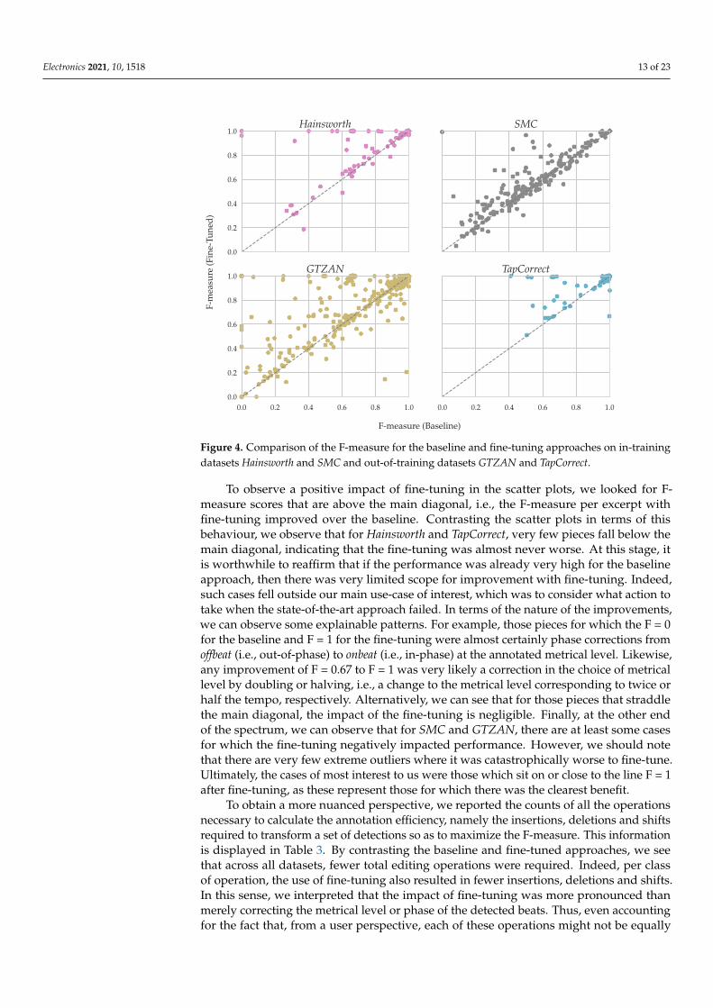
Inspection of Table 2 demonstrates that the inclusion of fine-tuning exceeded theperformance of the baseline state-of-the-art approach for all datasets—even accounting forthe deterministic choice of region for fine-tuning. However, while some broad interpreta-tion could be made by observing accuracy scores at the level of datasets, we could betterunderstand the impact of the fine-tuning via a scatter plot of the baseline vs. the fine-tunedF-measure per excerpt and per dataset, as shown in Figure 4.

Electronics 2021, 10, 1518 13 of 23

0.0

0.2

0.4

0.6

0.8

1.0Hainsworth SMC

0.0 0.2 0.4 0.6 0.8 1.00.0

0.2

0.4

0.6

0.8

1.0GTZAN

0.0 0.2 0.4 0.6 0.8 1.0

TapCorrect

F-measure (Baseline)

F-m

easu

re(F

ine-

Tune

d)

Figure 4. Comparison of the F-measure for the baseline and fine-tuning approaches on in-trainingdatasets Hainsworth and SMC and out-of-training datasets GTZAN and TapCorrect.

To observe a positive impact of fine-tuning in the scatter plots, we looked for F-measure scores that are above the main diagonal, i.e., the F-measure per excerpt withfine-tuning improved over the baseline. Contrasting the scatter plots in terms of thisbehaviour, we observe that for Hainsworth and TapCorrect, very few pieces fall below themain diagonal, indicating that the fine-tuning was almost never worse. At this stage, itis worthwhile to reaffirm that if the performance was already very high for the baselineapproach, then there was very limited scope for improvement with fine-tuning. Indeed,such cases fell outside our main use-case of interest, which was to consider what action totake when the state-of-the-art approach failed. In terms of the nature of the improvements,we can observe some explainable patterns. For example, those pieces for which the F = 0for the baseline and F = 1 for the fine-tuning were almost certainly phase corrections fromoffbeat (i.e., out-of-phase) to onbeat (i.e., in-phase) at the annotated metrical level. Likewise,any improvement of F = 0.67 to F = 1 was very likely a correction in the choice of metricallevel by doubling or halving, i.e., a change to the metrical level corresponding to twice orhalf the tempo, respectively. Alternatively, we can see that for those pieces that straddlethe main diagonal, the impact of the fine-tuning is negligible. Finally, at the other endof the spectrum, we can observe that for SMC and GTZAN, there are at least some casesfor which the fine-tuning negatively impacted performance. However, we should notethat there are very few extreme outliers where it was catastrophically worse to fine-tune.Ultimately, the cases of most interest to us were those which sit on or close to the line F = 1after fine-tuning, as these represent those for which there was the clearest benefit.

To obtain a more nuanced perspective, we reported the counts of all the operationsnecessary to calculate the annotation efficiency, namely the insertions, deletions and shiftsrequired to transform a set of detections so as to maximize the F-measure. This informationis displayed in Table 3. By contrasting the baseline and fine-tuned approaches, we seethat across all datasets, fewer total editing operations were required. Indeed, per classof operation, the use of fine-tuning also resulted in fewer insertions, deletions and shifts.In this sense, we interpreted that the impact of fine-tuning was more pronounced thanmerely correcting the metrical level or phase of the detected beats. Thus, even accountingfor the fact that, from a user perspective, each of these operations might not be equally

Electronics 2021, 10, 1518 14 of 23

easy to perform, and a reduction across all operation classes highlighted the potential forthe improved efficiency of an annotation-correction workflow.

Table 3. Global number of atomic edit operations: correct detections (#det), insertions (#ins), deletions(#del), shifts (#shf) and total edit operations (#ops) for the different test datasets.

Dataset Model #det #ins #del #shf #ops

Hainsworth Baseline 16,498 923 455 837 2215Fine-Tuned 17,241 500 246 517 1263

SMC Baseline 4593 810 1337 2457 4604Fine-Tuned 5028 670 1107 2162 3939

GTZAN Baseline 33,505 3348 1132 2235 6715Fine-Tuned 35,403 1911 492 1774 4177

TapCorrect Baseline 35,072 3285 1622 910 5817Fine-Tuned 36,659 2115 1236 493 3844

6.3. Impact on Individual Excerpts

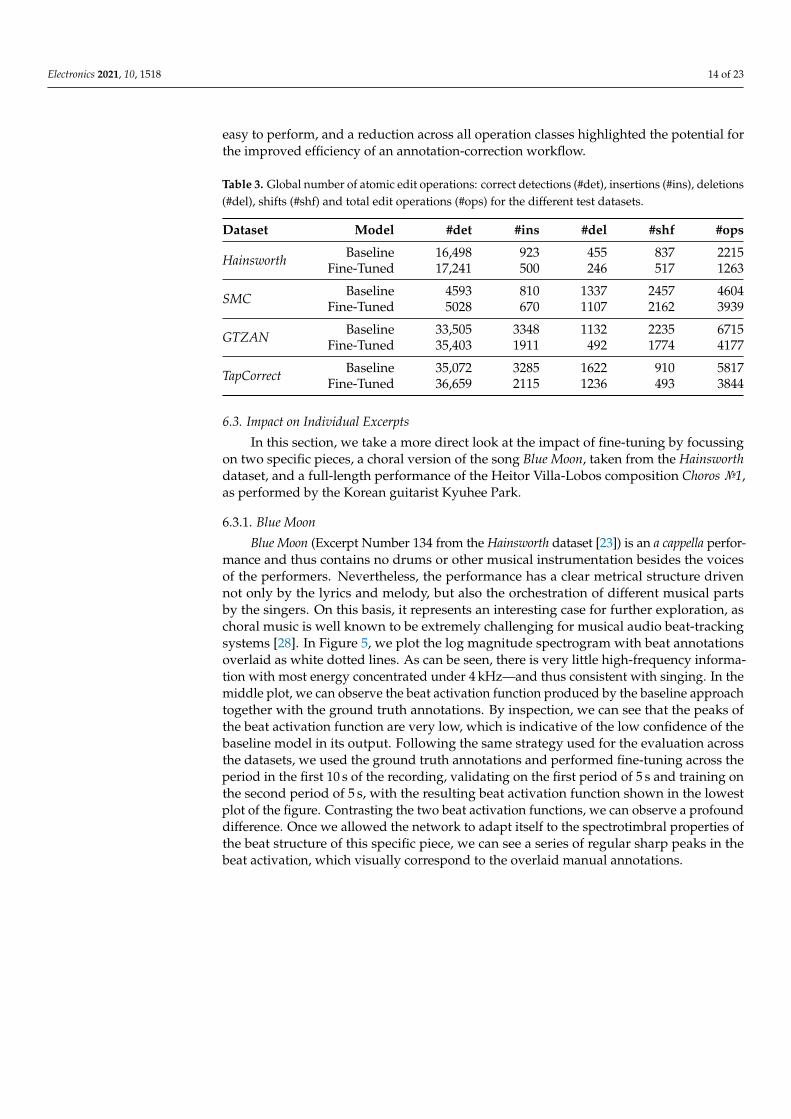
In this section, we take a more direct look at the impact of fine-tuning by focussingon two specific pieces, a choral version of the song Blue Moon, taken from the Hainsworthdataset, and a full-length performance of the Heitor Villa-Lobos composition Choros №1,as performed by the Korean guitarist Kyuhee Park.

6.3.1. Blue Moon

Blue Moon (Excerpt Number 134 from the Hainsworth dataset [23]) is an a cappella perfor-mance and thus contains no drums or other musical instrumentation besides the voicesof the performers. Nevertheless, the performance has a clear metrical structure drivennot only by the lyrics and melody, but also the orchestration of different musical partsby the singers. On this basis, it represents an interesting case for further exploration, aschoral music is well known to be extremely challenging for musical audio beat-trackingsystems [28]. In Figure 5, we plot the log magnitude spectrogram with beat annotationsoverlaid as white dotted lines. As can be seen, there is very little high-frequency informa-tion with most energy concentrated under 4 kHz—and thus consistent with singing. In themiddle plot, we can observe the beat activation function produced by the baseline approachtogether with the ground truth annotations. By inspection, we can see that the peaks ofthe beat activation function are very low, which is indicative of the low confidence of thebaseline model in its output. Following the same strategy used for the evaluation acrossthe datasets, we used the ground truth annotations and performed fine-tuning across theperiod in the first 10 s of the recording, validating on the first period of 5 s and training onthe second period of 5 s, with the resulting beat activation function shown in the lowestplot of the figure. Contrasting the two beat activation functions, we can observe a profounddifference. Once we allowed the network to adapt itself to the spectrotimbral properties ofthe beat structure of this specific piece, we can see a series of regular sharp peaks in thebeat activation, which visually correspond to the overlaid manual annotations.

Electronics 2021, 10, 1518 15 of 23

0

25

50

75

Freq

uenc

y(b

ands

)

Input

0.0

0.2

0.4

Pred

icti

onOutput (Baseline)

predictionannotationsvalidationfinetunetest

0 10 20 30 40 50time (seconds)

0.0

0.2

0.4

Pred

icti

on

Output (Fine-Tuned)

Figure 5. Network outputs for the baseline and fine-tuning approaches on Blue Moon. The validationregion is composed by the 5 s after the first beat annotation (red), the finetune region by the following5 s (blue) and the test region starting immediately after and going until the end of the file (green).

In terms of quantifying the improvement, we can see in Table 4 that when we fine-tuned, the number of required editing operations fell from eighty-three to eight, thusdemonstrating the impact that a small number of annotations can have in transformingthe efficacy of the baseline network for challenging content. To see this effect visually, wecan plot precisely which operations are required and at which time instants both for thebaseline and fine-tuned approach, as shown in Figure 6. In the upper plot of the figure, wecan observe the high number of insertions, which is indicative of the baseline approachestimating a slower metrical level than the annotations. While it is possible to interpolate aset of beat detections to twice the tempo, this is only straightforward in cases where thetempo is largely constant. From the regions around 8 s–11 s and likewise from 25 s–32 s,there are numerous shift operations as well, indicating that the HMM was not able to makereliable beat detections in this region. By contrast, we see far fewer operations in the lowerplot with the fine-tuned beat activation function, all of which are shifts in the form of minortiming corrections. Indeed, close inspection of the region right at the end of the excerpt(beyond the 50 s mark) highlights an interesting facet that the peaks of the beat activationfunction are strong, but misaligned with the annotations. Listening back to the manualannotations and the source audio, we could confirm that these specific annotations weredrifting out of phase and should be corrected.

Table 4. Annotation efficiency (ae), correct detections (#det) and insertions (#ins), deletions (#del),shifts (#shf) and total edit operations (#ops) for Blue Moon.

ae #det #ins #del #shf #ops

Baseline 0.272 31 56 0 27 83Fine-Tuned 0.930 107 0 1 7 8

Electronics 2021, 10, 1518 16 of 23

0.0

0.3

Pred

icti

on

Output (Baseline)

0 10 20 30 40 50time (seconds)

0.0

0.3

Pred

icti

onOutput (Fine-Tuned)

prediction annotations validation finetune test

Shifts Deletions Insertions Detections

Figure 6. Network outputs for the baseline and fine-tuning approaches on Blue Moon. The validationregion is composed by the 5 s after the first beat annotation (red), the finetune region by the following5 s (blue) and the test region starting immediately after and going until the end of the excerpt (green).The dark blue solid line indicates the network prediction. The vertical grey dotted lines showthe ground truth annotations. The vertical light blue solid lines show the correct beat detections.The incorrect beat outputs are notated with the required operation colour (delete—orange, shift—pink,insert—green).

6.3.2. Choros №1

The Blue Moon example from the previous section was selected in part due to itschallenging musical properties, but also since it could be identified as among the excerptsfrom the Hainsworth dataset whose F-measure score was most improved by fine-tuning.In this section, we move away from excerpts in existing annotated datasets and insteadlook towards a simulation of our real-world use case. For this example, we chose a highlyexpressive solo guitar performance of the Heitor Villa-Lobos composition Choros №1 asperformed by Kyuhee Park (for reference, the specific performance can be found at thefollowing url: https://www.youtube.com/watch?v=Uj_OferFIMk (accessed 25 May 2021)).Rather than using a minute-long excerpt, we examined the piece in its full duration of4 m 51 s. A particular characteristic of this piece and something that is especially prominentin this specific performance is the extreme use of rubato—a property that is challengingfor musical audio beat-tracking systems since it diverges strongly from the notion of aregular pulse. Indeed, the ground truth annotation of this piece, conducted entirely byhand in Sonic Visualiser [58], was very time-consuming and required frequent reference tothe score to resolve ambiguities.

In Figure 7, we show the score representation of the beginning of the piece, includingthe anacrusis and the first complete bar. The anacrusis is important as it represents the mainmotif of the piece, recurring in several locations across its duration. It is composed of threesixteenth notes with fermata, indicating that the notes should be prolonged beyond thenormal duration—at the discretion of the performer. This notation instructs the performerto an almost ad libitum interpretation, which results in extensive rubato across the fullpiece. Within the recording, these three sixteenth notes are clearly sounded by plucking,and given the absence of other instruments, they would be straightforward to detect evenfor a naive energy-based onset detection scheme. However, in the recording, they last over4 s in duration and are thus highly problematic for beat tracking, because by reference tothe score, all three occur within one notated beat.

Electronics 2021, 10, 1518 17 of 23

Figure 7. Excerpt of the Choros №1 score (until the end of the first complete bar).

Since the analysis of this piece is not within the domain of annotated datasets,we adapted our fine-tuning strategy and expanded the region for fine-tuning to coverthe first 15 s of the piece without validation and used the maximum number of epochs.Besides this alteration, we left all other aspects of the fine-tuning process described inSection 4 identical.

In the plots in Figure 8, the occurrences of this musical phrase are clearly depicted bya pattern in the log magnitude spectrogram input of the network in conjunction with theabsence of beat annotations. The beat activation function of the baseline network outputshows a strong indication of beats at these locations, whereas when performing fine-tuning,the beat activation is close to zero across all occurrences of the motif, despite the existenceof clear onsets. In contrast to the Blue Moon example in which we observed the networkadapt to a specific kind of spectrotimbral pattern to convey the beat, here we find evidencethat the fine-tuning process has allowed the network to learn what is not the beat.

0

25

50

75

Freq

uenc

y(b

ands

)

Input

0.0

0.2

0.4

0.6

Pred

icti

on

Output (Baseline)predictionannotationsfinetunetest

0 50 100 150 200 250time (seconds)

0.0

0.2

0.4

0.6

Pred

icti

on

Output (Fine-Tuned)

Figure 8. Network input and outputs for the baseline and fine-tuning approaches on Choros №1.Finetune region 0–15 s (blue) and the test region starting at 15 s (green).

The adaptation produced by the fine-tuning process has a clear impact from a practicalpoint of view, as shown in Figure 9 and Table 5, with fewer editing operations required.From the zoomed in plot in Figure 9, we can see how well the fine-tuned network learnedto ignore the motif once it occurred again just after the 30 s point. Indeed, here we observea potential downside of the normally advantageous property of the HMM to fill gaps in aplausible way, as we see spurious detections from the fine-tuned network, which must bedeleted. This behaviour, while specific to this piece, indicates that for highly expressivemusic including pulse suspensions, it may be worthwhile to consider a piecewise use ofthe HMM to prevent these gaps from being filled, e.g., based on the manual selectionof temporal regions for inference, or in an automatic way by segmenting and excludingso-called “no beat” regions, as in [59].

Electronics 2021, 10, 1518 18 of 23

0.0

0.3

0.6

Pred

icti

on

Output (Baseline)

0 5 10 15 20 25 30 35 40time (seconds)

0.0

0.3

0.6

Pred

icti

onOutput (Fine-Tuned)

prediction annotations finetune test

Shifts Deletions Insertions Detections

Figure 9. Network outputs for the baseline and fine-tuning approaches on Choros №1 (zoomed overthe initial 40 s). Finetune region 0–15 s (blue) and the test region starting at 15 s (green). The dark bluesolid line indicates the network prediction. The vertical grey dotted lines show the ground truthannotations. The vertical light blue solid lines show the correct beat detections. The incorrect beatoutputs are noted with the required operation colour (delete—orange, shift—pink, insert—green) tocorrect the annotation.

Table 5. Annotation efficiency (ae), correct detections (#det) and insertions (#ins), deletions (#del),shifts (#shf) and total edit operations (#ops) for Choros №1.

ae #det #ins #del #shf #ops

Baseline 0.555 207 0 69 97 166Fine-Tuned 0.654 236 0 57 68 125

6.3.3. Catastrophic Forgetting

In the final part of our evaluation, we considered the impact of fine-tuning froma different perspective. Having established that fine-tuning is beneficial at the level ofindividual pieces, we now re-assess the performance of a fine-tuned network adapted to agiven piece on other data. To this end, we investigated the presence and extent of “catas-trophic forgetting.” Known also as catastrophic interference, catastrophic forgetting is awell-known problem for backpropagation-based models [60] and is characterized by thetendency of an artificial neural network to abruptly forget previously learned informationupon learning new information. Despite the sequential learning nature of our fine-tuningadaptation, this is merely episodic, as opposed to the continual acquisition of incrementallyavailable information, which is more commonly addressed in catastrophic interference [61].Nevertheless, it is of interest in the context of this work to examine what a fine-tuned net-work loses in terms of general knowledge about the beat when adapted to the properties ofa specific piece of music.

To explore this behaviour, we return to the Blue Moon excerpt from the Hainsworthdataset. Across the training epochs of this excerpt, we evaluated the performance of eachof the corresponding 24 models over the GTZAN and TapCorrect datasets. More specifically,for every epoch of the fine-tuning of Blue Moon, we saved the intermediate network andused it to estimate the beat in every excerpt of the GTZAN and TapCorrect datasets. In thisway, we repeated the evaluation over these datasets 24 separate times.

Thus far, we have shown that, for this piece, there is a dramatic improvement inthe F-measure once the fine-tuning has completed. However, we have not observed themanner in which the F-measure improves over the intermediate training epochs, nor howthe fine-tuning process (i.e., specific to this musical excerpt) impacts performance on other

Electronics 2021, 10, 1518 19 of 23

musical content. In the presence of catastrophic forgetting, we should expect some kindof inverse relationship in performance, with the improvement on Blue Moon coming atthe expense of that on GTZAN and TapCorrect. In Figure 10, we plot this relationship over24 epochs and indicate that early stopping occurs at Epoch 18.

1 5 10 15 20 24Fine-tuning epoch

0.3

0.4

0.5

0.6

0.7

0.8

0.9F-

mea

sure

earl

yst

op

Blue MoonGTZANTapCorrect

Figure 10. Evolution of F-measure during fine-tuning of Blue Moon on the GTZAN and TapCorrectdatasets. Solid lines correspond to the fine-tuned model and dotted lines to the baseline model.

From the inspection of Figure 10, we can observe a rather nonlinear, and indeednonmonotonic, increase in performance for Blue Moon. Between Epochs 15 and 16, there isa sudden jump in performance, after which the F-measure saturates above 0.90. Lookingat the performance across the annotated datasets, we can see that the performance forGTZAN is essentially unchanged, and for TapCorrect, the F-measure falls by fewer thanthree percentage points. While our analysis was limited to fine-tuning on a single excerpt,it would appear that there was a very limited drop in performance due to the adaptionof the network to Blue Moon. Indeed, if we considered that there were approximately116 k weights in the baseline model and that we gave the network a very small temporalobservation of 5 s, to which the network adapted with a reduced learning rate (one-fifthof the baseline training), we should perhaps not be surprised that a great proportion ofthe network weights remained unchanged. At this stage, we leave deeper analysis of thisaspect as a topic for future work.

7. Discussion and Conclusions

In this paper, we explored the use of excerpt-specific fine-tuning of a state-of-the-artbeat tracking system based on exposure to a very small annotated region. Across existingdatasets, we demonstrated that this approach can lead to improved performance overthe state of the art, and furthermore, we illustrated its potential to adapt to challengingconditions in terms of timbre and musical expression. We believe that the principalcontribution of this work was to demonstrate the potential of fine-tuning within a user-driven annotation workflow and thus to provide a path towards very accurate analysis onhighly challenging musical pieces. Within the wider context of beat tracking, we foreseethat this type of approach could be used as a means for rapid, semi-automatic annotationof musical pieces to expand the amount of challenging annotated data for training newapproaches. To this end, we will pursue the integration of our fine-tuning approach withina dedicated user interface for annotation, e.g., Sonic Visualiser [58].

In spite of the promising results obtained, it is important to recognise several limita-tions of our work and how they may be addressed in the future. First, our comparisonagainst the state of the art was arguably tilted in favour of the fine-tuned approach, sinceper excerpt, we essentially created a new model and compared it to a single general modeltrained over a large amount of data. That said, our evaluation was carefully designed toexclude the interaction of the trained part of the input signal at inference, and furthermore,we did not claim that our fine-tuned approach represents a new state of the art. We simplysought to demonstrate that fine-tuning can be successfully applied across a large amount

Electronics 2021, 10, 1518 20 of 23

and variety of musical material. Second, our evaluation was dependent on a rather arbi-trary selection of two 5 s regions for training and validation; of course, we can expect thatas we increase the duration of these regions, then we will likely obtain better performancefor the piece in question, but doing so would require increased annotation effort on thepart of the user, which we sought to minimize as much as possible. Indeed, in the limit, thiswould resolve to the user annotating the entire piece without any need for an automatedsolution at all.

Concerning the location of these regions, this was largely dictated by the goal ofproviding a “fair” comparison with the baseline network. A specific limiting factor ofthis deterministic assignment of the training region is that if the musical content in theremainder of the piece differs greatly from the information available for fine-tuning, thenwe should not expect it to be beneficial. To this extent, we may be underestimating theperformance of our approach.

Within a real-world context, we foresee two main differences: (i) the end-user couldchoose where to annotate and for what proportion of the piece; and (ii) it would likelybe advantageous not to exclude the region that has been exposed to the network at thetime of inference. Beyond the presence of sharp peaks in the beat activation function,the user-provided beat annotations could also be harnessed for a more content-specificparameterisation of the inference technique, e.g., by setting an appropriate tempo range orsome other parameterisation targeted for the presence of expressive timing [31]. As such,we believe that the real validation of our approach is not rooted in existing annotateddatasets, but in a future user study that investigates how this approach can aid the annota-tion workflow. At this stage, we considered such an evaluation premature and reliant onfirst establishing, in quantitative terms, that fine-tuning is viable. However, in the future,we intend to gain deeper insight into how this approach could be used for data annotation,as well as understanding the impact and effort of the different correction operations. At themoment, we treated insertions, deletions and shifts as if they were equal for the calculationof the annotation efficiency, but we recognise that this is a simplification.

From a technical perspective, our approach to fine-tuning could be advanced inseveral ways. In our current implementation, we diverted from common practice intransfer learning between different tasks, which typically freezes all but the very lastnetwork layers, and instead unfroze all layers. In particular, we believe this is beneficialwhen it comes to analysing music that is unfamiliar from a timbre perspective and thusrequires the adaptation of layers closer to the musical signal. However, we contend thatthere is significant potential to explore more advanced strategies including discriminativefine-tuning and gradual unfreezing [50], as well input-dependent fine-tuning, whichcould automatically determine which layers to fine-tune per target instance [62]. Whenconsidering the training regime, we also intend to explore novel ways in which the networkadaptation could observe the entire piece, e.g., via semi-supervised learning, and thusovercome the limitations associated with fine-tuning based only on a partial observation ofthe input. Finally, looking beyond the task of musical audio beat tracking, we hope thatour proposed fine-tuning methodology could be applied within other annotation-intensiveMIR tasks.

Author Contributions: Conceptualization, A.S.P., S.B., J.S.C. and M.E.P.D.; data curation, A.S.P.,S.B. and M.E.P.D.; formal analysis, A.S.P.; funding acquisition, J.S.C. and M.E.P.D.; investigation,A.S.P.; methodology, A.S.P., S.B. and M.E.P.D.; project administration, A.S.P. and M.E.P.D.; resources,A.S.P. and J.S.C.; software, A.S.P. and S.B.; supervision, M.E.P.D.; validation, A.S.P. and M.E.P.D.;visualization, A.S.P.; writing—original draft, A.S.P. and M.E.P.D.; writing—review and editing, A.S.P.,S.B., J.S.C. and M.E.P.D. All authors read and agreed to the published version of the manuscript.

Funding: António Sá Pinto is supported by the FCT—Foundation for Science and Technology, I.P.—under Grant SFRH/BD/120383/2016. This research was also supported by national funds throughthe FCT—Foundation for Science and Technology, I.P.—under the projects IF/01566/2015 andCISUC—UID/CEC/00326/2020 and by the European Social Fund, through the Regional OperationalProgram Centro 2020.

Electronics 2021, 10, 1518 21 of 23

Conflicts of Interest: The authors declare no conflict of interest.

AbbreviationsThe following abbreviations are used in this manuscript:

BLSTM Bidirectional long short-term memory modelDBN Dynamic Bayesian networkDNN Deep neural networkHMM Hidden Markov modelMIR Music information retrievalMIREX Music Information Retrieval Evaluation eXchangeSTFT Short-time Fourier transformTCN Temporal convolutional network

References1. Schlüter, J.; Böck, S. Improved musical onset detection with Convolutional Neural Networks. In Proceedings of the IEEE

International Conference on Acoustics, Speech and Signal Processing (ICASSP), Florence, Italy, 4–9 May 2014; pp. 6979–6983.[CrossRef]

2. Schreiber, H.; Müller, M. Musical tempo and key estimation using convolutional neural networks with directional filters.In Proceedings of the Sound and Music Computing Conference (SMC), Malaga, Spain, 28–31 May 2019; pp. 47–54.

3. Cemgil, A.T.; Kappen, B. Monte Carlo Methods for Tempo Tracking and Rhythm Quantization. J. Artif. Intell. Res. 2003, 18, 45–81.[CrossRef]

4. Hainsworth, S. Beat Tracking and Musical Metre Analysis. In Signal Processing Methods for Music Transcription; Klapuri, A.,Davy, M., Eds.; Springer US: Boston, MA, USA, 2006; pp. 101–129. [CrossRef]

5. Sethares, W.A. Rhythm and Transforms; Springer Science & Business Media: Berlin/Heidelberg, Germany, 2007.6. Müller, M. Tempo and Beat Tracking. In Fundamentals of Music Processing; Springer International Publishing: Berlin/Heidelberg,

Germany, 2015; pp. 303–353. [CrossRef]7. Stark, A.M.; Plumbley, M.D. Performance Following: Real-Time Prediction of Musical Sequences Without a Score. IEEE Trans.

Audio Speech Lang. Process. 2011, 20, 190–199. [CrossRef]8. Nieto, O.; Mysore, G.J.; Wang, C.i.; Smith, J.B.L.; Schlüter, J.; Grill, T.; McFee, B. Audio-Based Music Structure Analysis: Current

Trends, Open Challenges, and Applications. Trans. Int. Soc. Music. Inf. Retr. 2020, 3, 246–263. [CrossRef]9. Fuentes, M.; Maia, L.S.; Rocamora, M.; Biscainho, L.W.; Crayencour, H.C.; Essid, S.; Bello, J.P. Tracking beats and microtiming in

Afro-latin American music using conditional random fields and deep learning. In Proceedings of the 20th International Societyfor Music Information Retrieval Conference (ISMIR), Delft, The Netherlands, 4–8 November 2019; pp. 251–258.

10. Vande Veire, L.; De Bie, T. From raw audio to a seamless mix: creating an automated DJ system for Drum and Bass. EURASIP J.Audio Speech Music. Process. 2018, 2018. [CrossRef]

11. Davies, M.E.P.; Hamel, P.; Yoshii, K.; Goto, M. AutoMashUpper: Automatic Creation of Multi-Song Music Mashups. IEEE/ACMTrans. Audio Speech Lang. Process. 2014, 22, 1726–1737. [CrossRef]

12. Bello, J.; Duxbury, C.; Davies, M.; Sandler, M. On the Use of Phase and Energy for Musical Onset Detection in the ComplexDomain. IEEE Signal Process. Lett. 2004, 11, 553–556. [CrossRef]

13. Dixon, S. Onset detection revisited. In Proceedings of the 9th International Conference on Digital Audio Effects (DAFx), Montreal,QC, Canada, 18–20 September 2006; pp. 133–137.

14. Davies, M.E.P.; Plumbley, M.D. Context-Dependent Beat Tracking of Musical Audio. IEEE Trans. Audio Speech Lang. Process. 2007,15, 1009–1020. [CrossRef]

15. Klapuri, A.P.; Eronen, A.J.; Astola, J.T. Analysis of the meter of acoustic musical signals. IEEE Trans. Audio Speech Lang. Process.2006, 14, 342–355. [CrossRef]

16. Dixon, S. An Interactive Beat Tracking and Visualisation System. In Proceedings of the International Computer Music Conference(ICMC), Havana, Cuba, 17–22 September 2001; pp. 215–218.

17. Goto, M.; Muraoka, Y. A beat tracking system for acoustic signals of music. In Proceedings of the 2nd ACM International Conferenceon Multimedia (MULTIMEDIA ’94); ACM Press: New York, NY, USA, 1994; pp. 365–372. [CrossRef]

18. Ellis, D.P.W. Beat Tracking by Dynamic Programming. J. New Music Res. 2007, 36, 51–60. [CrossRef]19. Böck, S.; Schedl, M. Enhanced beat tracking with context-aware neural networks. In Proceedings of the 14th International

Conference on Digital Audio Effects (DAFx), Paris, France, 19–23 September 2011; pp. 135–139.20. Böck, S.; Krebs, F.; Widmer, G. A Multi-model Approach to Beat Tracking Considering Heterogeneous Music Styles. In

Proceedings of the 15th International Society for Music Information Retrieval Conference (ISMIR), Taipei, Taiwan, 27–31 October2014; pp. 603–608.

21. Krebs, F.; Sebastian, B.; Widmer, G. An Efficient State-Space Model for Joint Tempo and Meter Tracking. In Proceedings of the16th International Society for Music Information Retrieval Conference (ISMIR), Malaga, Spain, 26–30 October 2015; pp. 72–78.

Electronics 2021, 10, 1518 22 of 23

22. Böck, S.; Davies, M.E.P. Deconstruct, Analyse, Reconstruct: How To Improve Tempo, Beat, and Downbeat Estimation. InProceedings of the 21st International Society for Music Information Retrieval Conference (ISMIR), Montreal, QC, Canada,12–16 October 2020; pp. 574–582.

23. Hainsworth, S. Techniques for the Automated Analysis of Musical Audio. Ph.D. Thesis, University of Cambridge, Cambridge,UK, 2004.

24. Davies, M.E.P.; Degara, N.; Plumbley, M.D. Evaluation Methods for Musical Audio Beat Tracking Algorithms; Technical ReportOctober; Queen Mary University of London: London, UK, 2009.

25. Marchand, U.; Peeters, G. Swing Ratio Estimation. In Proceedings of the 18th International Conference on Digital Audio Effects(DAFx), Trondheim, Norway, 30 November–1 December 2015; pp. 423–428.

26. Krebs, F.; Böck, S.; Widmer, G. Rhythmic Pattern Modeling for Beat and Downbeat Tracking in Musical Audio. In Proceedingsof the 14th International Society for Music Information Retrieval Conference (ISMIR), Curitiba, Brazil, 4–8 November 2013;pp. 227–232.

27. Peeters, G. The Deep Learning Revolution in MIR: The Pros and Cons, the Needs and the Challenges. In Perception, Representations,Image, Sound, Music—Proceedings of the 14th International Symposium (CMMR 2019), Marseille, France, 14–18 October 2019; RevisedSelected Papers; Kronland-Martinet, R., Ystad, S., Aramaki, M., Eds.; Springer: Berlin/Heidelberg, Germany, 2021; Volume 12631,pp. 3–30. [CrossRef]

28. Holzapfel, A.; Davies, M.E.P.; Zapata, J.R.; Oliveira, J.L.; Gouyon, F. Selective sampling for beat tracking evaluation. IEEE Trans.Audio Speech Lang. Process. 2012, 20, 2539–2548. [CrossRef]

29. Grosche, P.; Müller, M.; Sapp, C.S. What Makes Beat Tracking Difficult? A Case Study on Chopin Mazurkas. In Proceedings ofthe 11th International Society for Music Information Retrieval Conference (ISMIR), Utrecht, The Netherlands, 9–13 August 2010;pp. 649–654.

30. Dalton, B.; Johnson, D.; Tzanetakis, G. DAW-Integrated Beat Tracking for Music Production. In Proceedings of the Sound andMusic Computing Conference (SMC), Malaga, Spain, 28–31 May 2019; pp. 7–11.

31. Pinto, A.S. Tapping Along to the Difficult Ones: Leveraging User-Input for Beat Tracking in Highly Expressive Musical Content.In Perception, Representations, Image, Sound, Music—Proceedings of the 14th International Symposium, CMMR 2019, Marseille, France,14–18 October 2019; Revised Selected Papers; Kronland-Martinet, R., Ystad, S., Aramaki, M., Eds.; Springer: Berlin/Heidelberg,Germany, 2021; Volume 12631, pp. 75–90. [CrossRef]

32. Pons, J.; Serra, J.; Serra, X. Training Neural Audio Classifiers with Few Data. In Proceedings of the IEEE International Conferenceon Acoustics, Speech and Signal Processing (ICASSP), Brighton, UK, 12–17 May 2019; pp. 16–20. [CrossRef]

33. Pan, S.J.; Yang, Q. A survey on transfer learning. IEEE Trans. Knowl. Data Eng. 2010, 22, 1345–1359. [CrossRef]34. van den Oord, A.; Dieleman, S.; Schrauwen, B. Transfer Learning by Supervised Pre-training for Audio-based Music Classification.

In Proceedings of the 15th International Society for Music Information Retrieval Conference (ISMIR), Taipei, Taiwan, 27–31 October2014; pp. 29–34.

35. Choi, K.; Fazekas, G.; Sandler, M.; Cho, K. Transfer learning for music classification and regression tasks. In Proceedings of the18th International Conference on Music Information Retrieval (ISMIR), Suzhou, China, 23–27 October 2017; pp. 141–149.

36. Burloiu, G. Adaptive Drum Machine Microtiming with Transfer Learning and RNNs. Extended Abstracts for the Late-Breaking Demo Session of the International Society for Music Information Retrieval Conference (ISMIR). 2020. Available online:https://program.ismir2020.net/static/lbd/ISMIR2020-LBD-422-abstract.pdf (accessed on 25 May 2021).

37. Fiocchi, D.; Buccoli, M.; Zanoni, M.; Antonacci, F.; Sarti, A. Beat Tracking using Recurrent Neural Network: A Transfer LearningApproach. In Proceedings of the 26th European Signal Processing Conference (EUSIPCO), Rome, Italy, 3–7 September 2018;pp. 1915–1919. [CrossRef]

38. Wang, Y.; Yao, Q.; Kwok, J.; Ni, L.M. Generalizing from a Few Examples: A Survey on Few-Shot Learning. arXiv 2019,arXiv:1904.05046.

39. Choi, J.; Lee, J.; Park, J.; Nam, J. Zero-shot learning for audio-based music classification and tagging. In Proceedings of the 20thInternational Society for Music Information Retrieval Conference (ISMIR), Delft, The Netherlands, 4–8 November 2019; pp. 67–74.

40. Dhillon, G.S.; Chaudhari, P.; Ravichandran, A.; Soatto, S. A Baseline for Few-Shot Image Classification. In Proceedings of the 8thInternational Conference on Learning Representations (ICLR), Addis Ababa, Ethiopia, 26–30 April 2020.

41. Manilow, E.; Pardo, B. Bespoke Neural Networks for Score-Informed Source Separation.arXiv 2020, arXiv:2009.13729.

42. Wang, Y.; Salamon, J.; Cartwright, M.; Bryan, N.J.; Bello, J.P. Few-Shot Drum Transcription in Polyphonic Music. In Proceedingsof the 21st International Society for Music Information Retrieval Conference (ISMIR), Montreal, QC, Canada, 12–16 October 2020;pp. 117–124.

43. Davies, M.E.P.; Böck, S. Temporal convolutional networks for musical audio beat tracking. In Proceedings of the 27th EuropeanSignal Processing Conference (EUSIPCO), A Coruna, Spain, 2–6 September 2019.

44. Böck, S.; Davies, M.E.P.; Knees, P. Multi-Task Learning of Tempo and Beat: Learning One To Improve the Other. In Proceedingsof the 20th International Society for Music Information Retrieval Conference (ISMIR), Delft, The Netherlands, 4–8 November2019; pp. 486–493.

45. Böck, S.; Krebs, F.; Widmer, G. Joint Beat and Downbeat tracking with recurrent neural networks. In Proceedings of the 17thInternational Society for Music Information Retrieval Conference (ISMIR), New York, NY, USA, 7–11 August 2016; pp. 255–261.

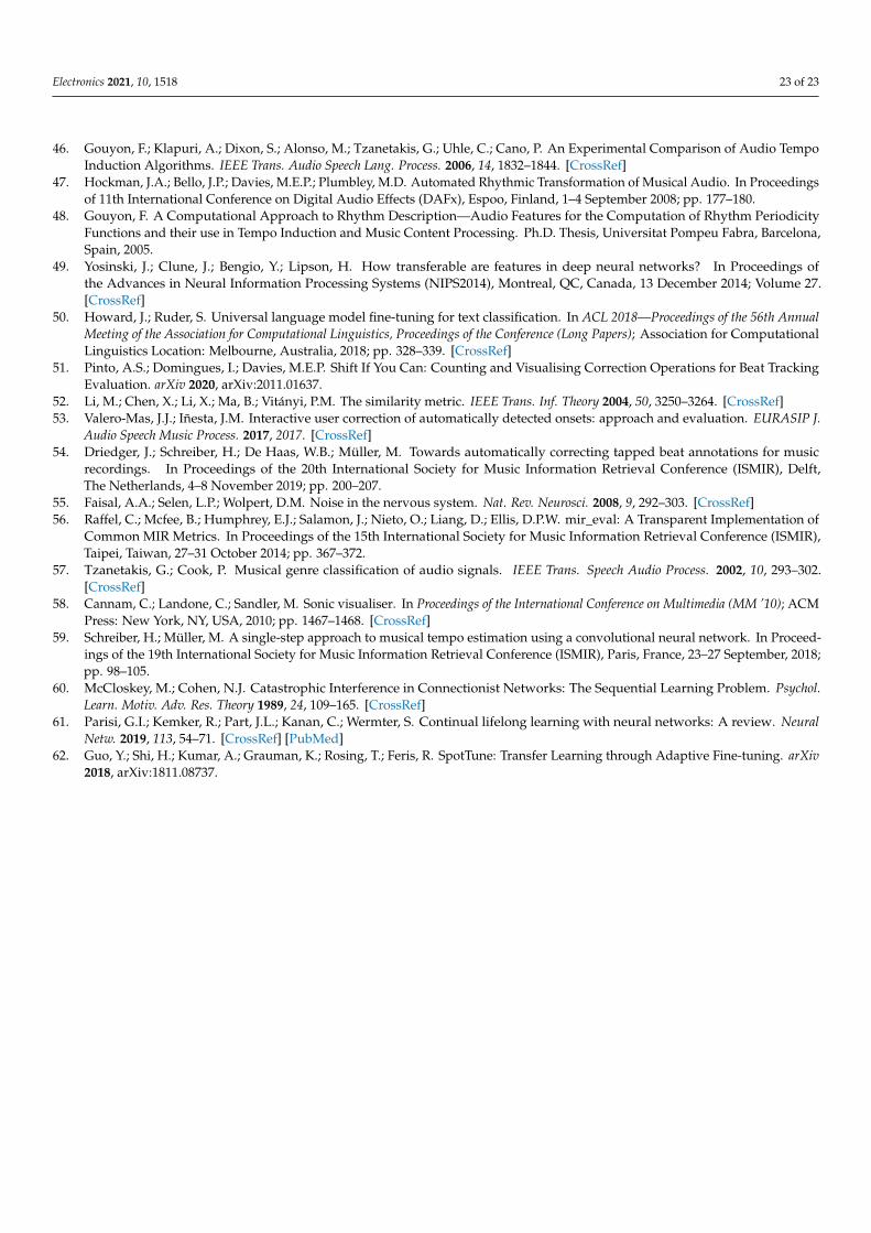
Electronics 2021, 10, 1518 23 of 23

46. Gouyon, F.; Klapuri, A.; Dixon, S.; Alonso, M.; Tzanetakis, G.; Uhle, C.; Cano, P. An Experimental Comparison of Audio TempoInduction Algorithms. IEEE Trans. Audio Speech Lang. Process. 2006, 14, 1832–1844. [CrossRef]

47. Hockman, J.A.; Bello, J.P.; Davies, M.E.P.; Plumbley, M.D. Automated Rhythmic Transformation of Musical Audio. In Proceedingsof 11th International Conference on Digital Audio Effects (DAFx), Espoo, Finland, 1–4 September 2008; pp. 177–180.

48. Gouyon, F. A Computational Approach to Rhythm Description—Audio Features for the Computation of Rhythm PeriodicityFunctions and their use in Tempo Induction and Music Content Processing. Ph.D. Thesis, Universitat Pompeu Fabra, Barcelona,Spain, 2005.

49. Yosinski, J.; Clune, J.; Bengio, Y.; Lipson, H. How transferable are features in deep neural networks? In Proceedings ofthe Advances in Neural Information Processing Systems (NIPS2014), Montreal, QC, Canada, 13 December 2014; Volume 27.[CrossRef]

50. Howard, J.; Ruder, S. Universal language model fine-tuning for text classification. In ACL 2018—Proceedings of the 56th AnnualMeeting of the Association for Computational Linguistics, Proceedings of the Conference (Long Papers); Association for ComputationalLinguistics Location: Melbourne, Australia, 2018; pp. 328–339. [CrossRef]

51. Pinto, A.S.; Domingues, I.; Davies, M.E.P. Shift If You Can: Counting and Visualising Correction Operations for Beat TrackingEvaluation. arXiv 2020, arXiv:2011.01637.

52. Li, M.; Chen, X.; Li, X.; Ma, B.; Vitányi, P.M. The similarity metric. IEEE Trans. Inf. Theory 2004, 50, 3250–3264. [CrossRef]53. Valero-Mas, J.J.; Iñesta, J.M. Interactive user correction of automatically detected onsets: approach and evaluation. EURASIP J.

Audio Speech Music Process. 2017, 2017. [CrossRef]54. Driedger, J.; Schreiber, H.; De Haas, W.B.; Müller, M. Towards automatically correcting tapped beat annotations for music

recordings. In Proceedings of the 20th International Society for Music Information Retrieval Conference (ISMIR), Delft,The Netherlands, 4–8 November 2019; pp. 200–207.

55. Faisal, A.A.; Selen, L.P.; Wolpert, D.M. Noise in the nervous system. Nat. Rev. Neurosci. 2008, 9, 292–303. [CrossRef]56. Raffel, C.; Mcfee, B.; Humphrey, E.J.; Salamon, J.; Nieto, O.; Liang, D.; Ellis, D.P.W. mir_eval: A Transparent Implementation of

Common MIR Metrics. In Proceedings of the 15th International Society for Music Information Retrieval Conference (ISMIR),Taipei, Taiwan, 27–31 October 2014; pp. 367–372.

57. Tzanetakis, G.; Cook, P. Musical genre classification of audio signals. IEEE Trans. Speech Audio Process. 2002, 10, 293–302.[CrossRef]

58. Cannam, C.; Landone, C.; Sandler, M. Sonic visualiser. In Proceedings of the International Conference on Multimedia (MM ’10); ACMPress: New York, NY, USA, 2010; pp. 1467–1468. [CrossRef]

59. Schreiber, H.; Müller, M. A single-step approach to musical tempo estimation using a convolutional neural network. In Proceed-ings of the 19th International Society for Music Information Retrieval Conference (ISMIR), Paris, France, 23–27 September, 2018;pp. 98–105.

60. McCloskey, M.; Cohen, N.J. Catastrophic Interference in Connectionist Networks: The Sequential Learning Problem. Psychol.Learn. Motiv. Adv. Res. Theory 1989, 24, 109–165. [CrossRef]

61. Parisi, G.I.; Kemker, R.; Part, J.L.; Kanan, C.; Wermter, S. Continual lifelong learning with neural networks: A review. NeuralNetw. 2019, 113, 54–71. [CrossRef] [PubMed]

62. Guo, Y.; Shi, H.; Kumar, A.; Grauman, K.; Rosing, T.; Feris, R. SpotTune: Transfer Learning through Adaptive Fine-tuning. arXiv2018, arXiv:1811.08737.