User clustering and traffic prediction in a trunked radio system
104
USER CLUSTERING AND TRAFFIC PREDICTION IN A TRUNKED RADIO SYSTEM Hao Leo Chen B.Eng., Zhejiang University, 1997 A THESIS SUBMITTED IN PARTIAL FULFILLMENT OF THE REQUIREMENTS FOR THE DEGREE OF MASTER OF SCIENCE in the School of Computing Science @ Hao Leo Chen 2005 SIMON FRASER UNIVERSITY Spring 2005 All rights reserved. This work may not be reproduced in whole or in part, by photocopy or other means, without the permission of the author.
Transcript of User clustering and traffic prediction in a trunked radio system

USER CLUSTERING AND TRAFFIC
PREDICTION IN A TRUNKED RADIO
SYSTEM
Hao Leo Chen
B.Eng., Zhejiang University, 1997
A THESIS SUBMITTED IN PARTIAL FULFILLMENT
OF THE REQUIREMENTS FOR THE DEGREE OF
MASTER OF SCIENCE in the School
of
Computing Science
@ Hao Leo Chen 2005
SIMON FRASER UNIVERSITY
Spring 2005
All rights reserved. This work may not be
reproduced in whole or in part, by photocopy
or other means, without the permission of the author.

APPROVAL
Name:
Degree:
Title of thesis:
Hao Leo Chen
Master of Science
User Clustering and Traffic Prediction in a Trunked
Radio System
Examining Committee: Dr. Arthur Kirkpatrick
Chair
Date Approved:
Dr. Ljiljana Trajkovid
Senior Supervisor
Dr. Martin Ester
Supervisor
Dr. Oliver Schulte
Supervisor
Dr. Qianping Gu
Examiner

SIMON FRASER UNIVERSITY
PARTIAL COPYRIGHT LICENCE
The author, whose copyright is declared on the title page of this work, has granted to Simon Fraser University the right to lend this thesis, project or extended essay to users of the Simon Fraser University Library, and to make partial or single copies only for such users or in response to a request from the library of any other university, or other educational institution, on its own behalf or for one of its users.
The author has further granted permission to Simon Fraser University to keep or make a digital copy for use in its circulating collection.
The author has further agreed that permission for multiple copying of this work for scholarly purposes may be granted by either the author or the Dean of Graduate Studies.
I t is understood that copying or publication of this work for financial gain shall not be allowed without the author's wrinen permission.
Permission for public performance, or limited permission for private scholarly use, of any multimedia materials forming part of this work, may have been granted by the author. This information may be found on the separately catalogued multimedia material and in the signed Partial Copyright Licence.
The original Partial Copyright Licence attesting to these terms, and signed by this author, may be found i n the original bound copy of this work, retained in the Simon Fraser University Archive.
W. A . C. Bennett Library Simon Fraser University
Burnaby, BC, Canada

Abstract
Traditional statistical analysis of network data is often employed to determine traf-
fic distribution, to summarize user's behavior patterns, or to predict future network
traffic. Mining of network data may be used to discover hidden user groups, to detect
payment fraud, or to identify network abnormalities. In our research we combine
traditional traffic analysis with data mining technique. We analyze three months of
continuous network log data from a deployed public safety trunked radio network. Af-
ter data cleaning and traffic extraction, we identify clusters of talk groups by applying
Autoclass tool and K-means algorithm on user's behavior patterns represented by the
hourly number of calls. We propose a traffic prediction model by applying the clas-
sical SARIMA models on the clusters of users. The predicted network traffic agrees
with the collected traffic data and the proposed cluster-based prediction approach
performs well compared to the prediction based on the aggregate traffic.

To my parents and my wife!

"The Tao is too great to be described by the name Tao.
If it could be named so simply, it would not be the eternal Tao."
- Tao Te Ching, LAO TZU

Acknowledgments
I am deeply indebted to my senior supervisor, Dr. Ljiljana Trajkovid, for her patient
support and guidance throughout this thesis. From her, I learned how to conduct
research and how to write research papers. It was a great pleasure for me to conduct
this thesis under her supervision.
I want to thank my supervisor Dr. Oliver Schulte for his valuable suggestions and
inspiring discussions on Bayesian learning approaches. I want to thank my supervisor
Dr. Martin Ester for his constructive comments about the clustering methods. I feel
obliged to thank Dr. Qianping Gu who read my thesis carefully and gave me advice on
thesis writing. The chair Dr. Arthur Kirkpatrick was of great help during my thesis
defense. The defense would not have gone so smoothly without his coordination.
I also want to express my sincere appreciation to all the members in our CNL
laboratory for their comments and suggestions on the thesis presentation, especially
Kenny Shao and James Song for the valuable discussions on the topic of data analysis
and prediction.

Contents
Approval
Abstract
Dedication
Quotat ion v
Acknowledgments vi
Contents vii
List of Tables x
List of Figures xi
1 Introduction 1
2 Data preparation 4 . . . . . . . . . . . . . . . . . . . . . . . . . . . . . 2.1 E-Comm network 4
. . . . . . . . . . . . . . 2.1.1 E-Comm network structure overview 4 . . . . . . . . . . . . . . . . . . 2.1.2 E-Comm network terminology 5
. . . . . . . . . . . . . . . . . . . . . . . . . . . 2.2 Network traffic Data 7 . . . . . . . . . . . . . . . . . . . . . . . . . . 2.2.1 Database setup 7
. . . . . . . . . . . . . . . . . . . . 2.2.2 Event log database schema 8 . . . . . . . . . . . . . . . . . . . . . . . . . . 2.2.3 Topic of interest 9
vii

. . . . . . . . . . . . . . . . . . . . . . . . . . . . 2.3 Data preprocessing
. . . . . . . . . . . . . . . . . . . . . . . . 2.3.1 Database shrinking
. . . . . . . . . . . . . . . . . . . . . . . . . 2.3.2 Database cleaning
. . . . . . . . . . . . . . . . . . . . . . . . . . . . . . 2.4 Data extraction
2.5 Summary . . . . . . . . . . . . . . . . . . . . . . . . . . . . . . . . .
3 Data analysis
. . . . . . . . . . . . . . . . . . . . . . . . 3.1 Analysis on Network level
. . . . . . . . . . . . . . . . . . . . . . . . . 3.2 Analysis on agency level
. . . . . . . . . . . . . . . . . . . . . . . 3.3 Analysis on talk group level
3.4 Summary . . . . . . . . . . . . . . . . . . . . . . . . . . . . . . . . .
4 Data clustering
. . . . . . . . . . . . . . . . . . . . 4.1 Data representing user's behavior
. . . . . . . . . . . . . . . . . . . . . . . . . . . . . . 4.2 AutoClass tool
. . . . . . . . . . . . . . . . . . . . . . . . . . . . 4.3 K-means algorithm
. . . . . . . . . . . . . . . . . 4.4 Comparison of AutoClass and K-means
. . . . . . . . . . . . . . . . . . . . . . . . . . . . . . . . . 4.5 Summary
5 Data prediction
. . . . . . . . . . . . . . . . . . . . . . . . . 5.1 Time series data analysis
. . . . . . . . . . . . . . . . . . . . . . . . . . . . . . 5.2 ARIMA model
. . . . . . . . . . . . . . . . . . . 5.2.1 Autoregressive (AR) models
. . . . . . . . . . . . . . . . . . 5.2.2 Moving average (MA) models
. . . . . . . . . . . . . 5.2.3 SARIMA (p, d, q) x (P. D. Q)s models
. . . . . . . . . . . . . . . . . . . . . 5.2.4 SARIMA model selection
. . . . . . . . . . . . . . . . . . 5.3 Prediction based on aggregate traffic
. . . . . . . . . . . . . . . . . . . . 5.4 Cluster-based prediction approach
. . . . . . . . . . . . . . . . . . . . . . . 5.5 Additional prediction results
5.5.1 Comparison of predictions with the (2,0, 1) x (0,1, model
5.5.2 Comparison of predictions with the (2,0, 1) x (0, 1 , 1) ls8 model
. . . . . . . . . . . . . . . . . . . . . . . . . . . . . . . . . 5.6 Summary
... Vll l

6 Conclusion 6 6
. . . . . . . . . . . . . . . . . . . . . . . . . 6.1 Related and future work 67 8
A D a t a table. SQL. a n d R scripts 6 8
. . . . . . . . . . . . . . . . . . . . . . . . . . . . . . A . 1 Call-Type table 68
. . . . . . . . . . . . . . . . . . . . A.2 SQL scripts for statistical output 69
. . . . . . . . . . . . A.3 R scripts for prediction test and result summary 69
. . . . . . . . . . . . . . . . . . . . A.3.1 R script for prediction test 69
. . . . . . . . . A.3.2 R script used to summarize prediction results 73
B Autoc lass files 76
. . . . . . . . . . . . . . . . . . . . . . . . . . . B.l Autoclass model file 76
. . . . . . . . . . . . . . . . . . . . B.2 Autoclass influence factor report 76
. . . . . . . . . . . . . . . . . . . B.3 Autoclass class membership report 80
C Bayesian network analysis 8 3
. . . . . . . . . . . . . . . . . . . . . . . . . . . . . C.l B-Course analysis 83
. . . . . . . . . . . . . . . . . . . . . . . . . . . . . . C.2 Tetrad analysis 83
Bibliography 8 8

List of Tables
Number of records per day: original vs . cleaned database . . . . . . . 13
A sample of cleaned data . . . . . . . . . . . . . . . . . . . . . . . . . 15
A sample of extracted traffic data . . . . . . . . . . . . . . . . . . . . . 17
Agency network usage . . . . . . . . . . . . . . . . . . . . . . . . . . . 23
Sample of the resource consumption for various talk groups . . . . . . 26
Sample of hourly number of calls for various talk groups . . . . . . . . 31
Autoclass results: 10 best clusters . . . . . . . . . . . . . . . . . . . . 35
Autoclass results: cluster sizes . . . . . . . . . . . . . . . . . . . . . . 35
K-means results: cluster size and distances . . . . . . . . . . . . . . . 39
Comparison of talk group calling properties (AC: Autoclass, K: K-
means. nc: number of calls) . . . . . . . . . . . . . . . . . . . . . . . . 41
Summary of SARIMA models fitting measurement . . . . . . . . . . . 49
Aggregate-traffic-based prediction results . . . . . . . . . . . . . . . . . 55
Summary of the results of cluster-based prediction . . . . . . . . . . . 58
Comparison of predictions with (2.0. 1) x (0.1. model: part 1 . . . 61
Comparison of predictions with (2.0. 1) x (0.1. model: part 2 . . 62
Comparison of predictions with (2.0. 1) x (0.1. model: part 1 . . 63
Comparison of predictions with (2.0. 1) x (0.1. model: part 2 . . 64

List of Figures
E-Comm network coverage in the Greater Vancouver Regional District.
Algorithm for extracting traffic data. . . . . . . . . . . . . . . . . . .
Comparison of number of records in original, cleaned, and extracted
databases. . . . . . . . . . . . . . . . . . . . . . . . . . . . . . . . . .
Statistical analysis of hourly (top) and daily (bottom) number of calls.
Fast Fourier Transform (FFT) analysis on hourly (top) and daily (bot-
tom) number of calls. The high frequency components a t 24 (top) and
7 (bottom) indicate that the network traffic exhibits daily (24 hours)
and weekly (168 hours) cycles, respectively. . . . . . . . . . . . . . . .
Traffic analysis by agencies (Top: the daily number of calls for each
agency. Middle: the daily average call duration of each agency. Bot-
tom: the average number of systems involved in the calls of each agency.
Calling patterns for talk groups 1 (top) and 2 (bottom) over the 168-
hour period. . . . . . . . . . . . . . . . . . . . . . . . . . . . . . . . .
Calling patterns for talk groups 20 (top) and 263 (bottom) over the
168-hourperiod . . . . . . . . . . . . . . . . . . . . . . . . . . . . . . .
Sample of the Aut,oClass header file. . . . . . . . . . . . . . . . . . .
Number of calls for three Autoclass clusters with IDS 5 (top), 17 (mid-
dle), and 22 (bottom). . . . . . . . . . . . . . . . . . . . . . . . . . .
K-means result: number of calls in three clusters. . . . . . . . . . . .
Definition of the autoregressive (AR) model. . . . . . . . . . . . . .

5.2 Definition of the moving average (MA) model . . . . . . . . . . . . . . 45
5.3 Definition of the ARIMA/SARIMA model . . . . . . . . . . . . . . . . 46
5.4 Auto-correlation function and Partial auto-correlation function . . . . 48
5.5 Residual analysis: diagnostic test for model (3,0, 1) x (0.1. . . . . 51
5.6 Residual analysis: diagnostic test for model (1.1. 0) x (0.1. . . . . 52
. . . . . . . . 5.7 Number of calls: sample auto-correlation function (ACF) 53
5.8 Number of calls: sample Partial auto-correlation function (PACF) . . 54
5.9 Predicbing 168 hours of traffic data based on the 1. 680 past data . . . 57
C.l B-Course analysis: result 1 . . . . . . . . . . . . . . . . . . . . . . . . 84
C.2 B-Course analysis: result 2 . . . . . . . . . . . . . . . . . . . . . . . . 85
C.3 Tetrad analysis: result 1 . . . . . . . . . . . . . . . . . . . . . . . . . . 86
C.4 Tetrad analysis: result 2 . . . . . . . . . . . . . . . . . . . . . . . . . . 87
xii

Chapter 1
Introduction
Analysis of traffic from operational wireless networks provides useful information
about the network and users' behavior patterns. This information enables network
operators to better understand the behavior of network users, to better use network
resources, and, ultimately, to provide better quality of services.
Traffic prediction is important in assessing future network capacity requirements
and in planning network development. Traditional prediction of network traffic usually
considers aggregate traffic from individual network users. It also assumes a constant
number of network users. This approach cannot easily adapt to a dynamic network
environment where the number of users varies. An alternate approach that focuses
on individual users is impractical in predicting the aggregate network traffic because
of the high computational cost in cases where the network consists of thousands of
users. Employing clustering technique for predicting aggregate network traffic bridges
the apparent gap between these two approaches.
Data clustering may be used to identify and define customer groups in various
business environments based on their purchasing patterns. In the telecommunica-
tion industry, clustering techniques may be used to identify traffic patterns, detect
fraudulent activities, and discover users' mobility patterns. Network users are usually
classified into user groups according to geographical location, organizational structure,
payment plan, or behavior pattern. Patterns of users' behavior reflect the nature of

CHAPTER 1. INTRODUCTION 2
user activities and, as such, are inherently consistent and predictable. However, em-
ploying users' behavior patterns to classify user groups and to predict network traffic
is non-trivial.
In this thesis, we analyze traffic data collected from a deployed network. We use
hourly number of calls to represent individual user's calling behavior. We then predict
network traffic based on the aggregate traffic and based on the identified clusters of
users. Experimental results show that the cluster-based prediction produces results
comparable to the traditional prediction of network traffic. The user cluster based
traffic prediction approach may also address the computational cost and the dynamic
number of users problems. An advantage of cluster-based prediction is that it may
be used for predictions in networks with variable number of users. This approach
provides a balance between a micro and a macro view of a network.
This thesis includes additional five chapters.
Chapter 2 begins with a brief introduction to the network and the t,raffic data that
we analyzed. It is followed by the description of data preprocessing, data extraction
and the results.
In Chapter 3, various statistical analysis routines have been applied to the traffic
data on three levels: network, agency, and talk group levels. The analysis results
include plots and basic statistical measures (maximum, minimum, mean value, and
variance).
In Chapter 4, we discuss the general clustering techniques and principles. We
apply the AutoClass clustering tool and K-means algorithm to classify talk groups
into clusters based on their calling activities. We also compare the the clustering
results of AutoClass and K-means.
In Chapter 5, we present the Seasonal Autoregressive Integrated Moving Average
(SARIMA) time series prediction model. We discuss the model selection method and
present the prediction results of the network traffic. We conclude with a comparison of
the prediction results of cluster-based models and models based on aggregate traffic.
We conclude the thesis with Chapter 6. A short summary of experiences that we
gained is given and the future work is addressed.
Appendics include additional database tables, SQL scripts, R scripts, and snippets

CHAPTER 1. INTRODUCTION 3
of Autoclass model and report files. Experimental results of conditional dependency
analysis of the traffic data using Bayesian network are also presented.

Chapter 2
Data preparation
The traffic data analyzed in this thesis were obtained from E-Comm [I]. In this Chap-
ter, we first introduce the architecture of the E-Comm network and the underlying
technology. We also examine the database schema and describe the procedure for
data cleaning and the traffic data extraction.
2.1 E-Comm network
2.1.1 E-Comm network structure overview
EComm is the regional emergency communications center for Southwest British
Columbia, Canada. It provides emergency dispatch/communication services for a
number of police and fire departments in t,he Greater Vancouver Regional District
(GVRD), the Sunshine Coast Regional District, and the Whistler/Pemberton area.
E-Comm serves sixteen agencies such as Royal Canadian Mounted Police (RCMP),
fire and rescue, local police departments, ambulance, and industrial customers such
as BC Translink [2]. Each agency has a number of affiliated t,alk groups and the entire
network serves 617 talk groups. Figure 2.1 presents a rough geographical coverage of
the E-Comm network.
Before the establishment of EComm, ambulance, fire, and police agencies could
not communicate with each ot,her effectively because they used separate radio systems.

CHAPTER 2. DATA PREPARATION 5
The deployment of the E-Comm network in 1999 provided an integrated shared com-
munications infrastructure to various emergence service agencies. It enables the cross
communication between various agencies and municipalities.
The EComm network employs Enhanced Digital Access Communications System
(EDACS), developed by MIA-COM [3] (formerly Comnet-Ericsson) in 1988. EDACS
system is a group-oriented communication system that allows groups of users to com-
municate with each other regardless of their physical locations. The main advantages
of this approach are improved coordinat,ion, efficient exchange of information, and
efficient resource usage.
The E-Comm network consists of 11 cells. Each cell covers one or more munici-
palities, such as Vancouver, Richmond, and Burnaby. Identical radio frequencies are
transmitted within one cell using multiple repeaters. This is known as simulcast. The
basic talking unit in the trunked radio network is a talk group: a group of individ-
ual users working and communicating with each other to accomplish certain tasks.
Although the E-Comm network is capable of both voice and data transmissions, we
analyze only voice traffic because it accounts for more than 99% of the network traffic.
2.1.2 E-Comm network terminology
We explain briefly the following network terms:
System/Cell: A trunked radio network is divided into smaller areas in order to
reuse the radio frequencies and to increase the network capacities. One system
represents one service area and a cell is the synonymous of a system. One system
could serve one or more municipalities, based on the frequencies availability and
geographical connection. A unique system id is associated with each system.
Within a system/cell, the radio signal is transmitted using the same range of
frequencies.
Channel: A channel is a small range of radio frequencies or a time slot. Various
numbers of channels are assigned in each system based on the traffic throughput

CHAPTER 2. DATA PREPARATION
l sland
0 Police
a Ambulance
@ Fire
Figure 2.1: E-Comm network coverage in the Greater Vancouver Regional District.
and the system needs. Two types of radio channel are used in EDACS: control
and traffic channels. There is one control channel in each cell, while the remain-
ing channels are used as traffic channels. The control channel is used to send
protocol messages between radios and the base station equipment for controlling
the operation of the system. Traffic channels are used to transmit the voice or
data messages between radios or between radios and the base stations.
Group Call: Group call is the typical call made in a trunked radio system. A group
is a set of users who need to communicate regularly in order to accomplish
certain tasks. For example, within a single city-wide system, the North and
South fire services may each have one talk group, while the police may be
subdivided into several talk groups. A user only needs to press the push-to-talk
(PTT) button on the radio device to initiate a group call. All users belonging to

CHAPTER 2. DATA PREPARATION 7
the same talk group will hear the communications in the group call irrespective
of their physical locations. Most EDACS network operators have observed that
more than 85% of calls are group calls [4].
Simulcast: In the E-Comm network, simulcast is used in a single cell. Within a cell,
identical radio frequencies are transmitted simultaneously between two or more
base station sites in order to improve signal strength and increase coverage.
Multi-System Call: It represents a single group call involving more than one
system/cell. A user may initiate a group call without knowing the physical
location of the group members. When all members of the talk group reside
within one system, the group call is a single-system call occupying only one
traffic channel in the system. However, when group members are distributed
over multiple systems, the group call becomes a multi-system call that occupies
one traffic channel in each system. Hence, the major difference between a multi-
system call and a single-system call is that the first occupies additional channels
and consumes more system resources. In the collected traffic data, more than
55 % of group calls are multi-system calls.
Network traffic Data
The traffic data received from EComm contains event log tables recording the activ-
ities occurred in the network. They are aggregated from the distributed database of
the network management systems.
2.2.1 Database setup
Analyzed data records span from 2003-03-01 00:00:00 to 2003-05-31 23:59:59 contin-
uously. The database size is -- 6G bytes, with 44,786,489 records for the 92 days of
data. It consists of 92 event log tables, each containing one data's events generated
in the network, such as the call establishment, call drop, and emergency call events.
Its sheer volume was one of the main difficulties in our data analysis. For efficiency,

CHAPTER 2. DATA PREPARATION 8
we converted the data from the MS Access format to plain text files and imported
the records into the MySQL [5] database server under Linux platform.
2.2.2 Event log database schema
The complete twenty-six data fields in the event log table are:
1. Event-UTC-At: the timestamp of the event (granularity is 3 ms).
2. Duration$ms: the duration of the event in ms (granularity is 10 ms).
3. Network-Id: the identification of the network (constant in t,he database).
4. Nodeld: the identification of the net,work node (not populated)
5. Systemld: the identification of the system/cell involved in the event, ranging
from 1 to 11.
6. Channel-Id: the identification of the channel involved in the event.
7. Slotld: this field is not populated in the database.
8. Caller: also known as LID (Logic ID). It is the caller's id, ranging from 1 to
16!000. The first 2,000 LIDs are assigned to either talk groups or individual
users. The remaining LIDs are assigned to talk groups only.
9. Callee: the callee's id in the event, having the same value range as Caller.
10. Call-Type: the type of the call, such as group call, emergency call, and individual
call.
11. CallState: the state of the call event, such as assign channel, drop, and queue.
12. Call-Direction: the direction of the call (meaning unknown).
13. Voice-Call: a flag indicat,ing a voice call.
14. DigitalLCall: a flag indicating a digital call.

CHAPTER 2. DATA PREPARATION 9
15. Interconnect-Call: a flag indicating a call interconnecting the EDACS and the
Public Switched Telephone Network (PSTN).
16. Multi-System-Call: a flag indicating a multi-system call. It is only set in the
event of call drop.
17. Confirmed-Call: a flag of the call. A call is a confirmed call when every member
of a talk group has to confirm the call before the conversation begins.
18. Msg-Trunked-Call: a flag of the call (meaning unknown).
19. Preempt-Call: a flag of the call. A preempt-call has higher queue priority.
20. Primary-Call: a flag of the call (meaning unknown).
21. Queue-Depth: the depth of the current system queue at the event moment. It
may be used to investigate the block rate of the system.
22. Queue-Pri: the priority number of the call in queue.
23. MCP (Multi-Channel-Partition): the partition number of channels (not popu-
lated).
24. Caller-Bill: set to 1 if the call is billable to the caller (not used in the current
system).
25. Callee-Bill: set to 1 if the is billable to the callee (not used in the current
system).
26. Reason-Code: the error reason code number, providing additional information
if any error occurs during the call.
2.2.3 Topic of interest
Two open questions, emanating from the discussions with E-Comm staff and the
analysis of database, are of particular interest to our analysis: the precise measurement
of network usage per agency and the traffic forecast based on user's behavior patterns.

CHAPTER 2. DATA PREPARATION 10
A. Precise measurement of network usage
The current billing policy for agencies in the E-Comm network is based on the
geographic coverage arid the approximate calling traffic volurne of each agency. Traffic
volume factors are further broken down into the number of radios, radio t,raffic! arid
user population. Shared radio infrastructure costs are allocated based on the coverage
area, number of radios, radio traffic, and population.
PresentJy, there is no precise measuring method for t,he t,raffic generated by each
individual user/talk group. The current database is an event log database, recording
every activity that occurred in the network, such as the call establishment, call drop,
and emergency calls. One group call may be recorded twice in the event log, as it
generates both call assignment and call drop events. One single multi-system call
involving several systems generates multiple entries in the database. Based solely
on the raw t.raffic logs, the calculation of network resources used by one agency is
inaccurate. Therefore, the t,raffic generated by agencies is not calculated directly
from the event database. It is, instead, based on an assumed mean value of call
duration, the coverage of cells by the agency, the number of radios possessed by the
agency, and the number of records corresponding to the agency. It is unable to identify
the number of calls made by each agency, the average/maximum number of systems
involved in calls for each agency, and the network usage for each talk group. A sample
of the data is shown in Section 2.4.
B. Traffic forecast based on user's behavior patterns
Users' behavior patterns in the trunked radio networks are different from the tradi-
tional telephone networks. Group calls involve more than two users, while traditional
telephone calls connect only two persons. Furthermore, since the E-Comm network
mainly serves emergency communications, the uncertainty of emergencies implies dif-
ferent behavior patterns of network users from users of ordinary telephone network.
In addition, different agencies may have different behavior patterns. For example,
the ambulance service may have different peak hours from the RCMP, while the fire
de~art~ment often dispatch group of firefighters tto the accident sites together with the
police groups.
CHAPTER 2. DATA PREPARATION 11
Understanding user's behavior could help improve user satisfaction and be ben-
eficial for the network optimization and the planning for network expansion. For
example, if a police department plans to increase its manpower by increasing the pa-
trol groups and using more radios. A reasonable assumption is that the new groups
have similar behavior patterns to the existing users. New patrol groups may be clas-
sified into certain existing user groups based on their behavior patterns. Considering
the number of new members in the user groups, we may forecast the net,work t,raffic
based on the existing user's behavior patterns, thus to make better assessment on the
network capacity.
2.3 Data preprocessing
The main difficulty in analyzing the network log data is the sheer volume of data.
Data preprocessing is the fundamental and mandatory step for data analysis. It is
used to clean the database and filter the outliers and redundant records. The current
database includes: surplus data fields wit,h useless entries, obscure data records, and
inconsistent data fields. The goals of the data preprocessing step are to remove useless
information and to remove the outliers. They are accomplished by acquiring the
necessary domain knowledge from the system documentation and via interviews with
the E-Comm staff. The preprocessing procedure is composed of database shrinking
and cleaning.
2.3.1 Database shrinking
Not all data fields are useful to our analysis. Certain fields are not populated in
the database (Nodeld and Slot-Id fields), while others have identical value or are
unrelated to our research (Network-Id, Caller-Bill, and Callee-Bill). We are only in-
terested in fields t,hat could capture the user's behavior and network t,raffic. Thus, the
step is to remove these unpopulated, identical, or unrelated fields from the database,
such as the Digital-Call, Interconnect-Call, Confirmed-Call, Primary-Call, Caller-Bill,
Callee-Bill, and Reason-Code fields.
CHAPTER 2. DATA PREPARATION 12
From the twenty-six original fields in the database, nine fields are of particular
interest to our analysis: 1) Event-UTC-At, 2) Duration$ms, 3) System-Id, 4) Chan-
nel ld, 5) Caller, 6) Callee, '7) Call-Type, 8) Call-State, and 9) Multi-System-Call.
2.3.2 Database cleaning
After reducing the database dimension to nine, we removed redundant records, such as
records having call-type = 100 or records with duration = 0. Records with callstate
= 1, which implies the call drop event, are redundant because each call drop event
already has a corresponding call assignment event in the database. (Note that the
reverse is not true.) Records with channel-id = 0 should also be removed as well
because the channel id 0 represents the control channel whose traffic we have not
considered. We keep the the records with call-type = 0, 1, 2, or 10, representing
group call, individual call, emergency call, and start-emergency-call, respectively. The
complete call-type table is given in Appendix A.
The result of data preprocessing step is a smaller and cleaner database. The
number of records in each data table of original and cleaned databases are compared in
Table 2.1. Approximately 55% records have been removed from the original database
after preprocessing. Furthermore, due to the effect of the dimension reduction, the
total size of the database has been reduced to only 19% of the original size.
2.4 Data extraction
The extract,ion of the network traffic may solve the first open question of imprecise
traffic measurement, as described in Section 2.2.3. A sample of the cleaned database
table is shown in Table 2.2. If a call is a multi-system call involving several systems,
several records (one for each involved system) are created to represent this call in the
original event log database. For example, based on the caller, callee, and duration
information, records 1 and 6 represent one group call from caller 13905 to callee 401,
involving systems 1 and 7 and lasting 1350 ms. Records 29, 31, 37, and 38 represent
a group call from caller 13233 to callee 249, involving systems 2, 1, 7, and 6. Thus, the

Da
te
Ori
gin
al
Cle
aned
20
03/0
3/01
46
6.86
2 20
4.35
7
2003
/03/
31
-,
~
Tot
al:
16,0
12,4
32
7,25
7,50
2
Da
te
Ori
gin
al
Cle
aned
20
03/0
4/01
57
8,83
4 26
0,75
2
Tot
al:
13,7
21,2
36
6,12
9,55
0
Dat
e O
rigi
nal
C
lean
ed
2003
/05/
01
535,
919
240,
046
, ,
Tot
al:
15.0
52.8
21
6.74
3.66
6
Tab
le 2
.1:
Num
ber
of
reco
rds
per
day:
ori
gina
l vs.
cle
aned
dat
abas
e.

CHAPTER 2. DATA PREPARATION 14
network operator cannot count the number of group calls made by a certain talk group
or agency merely based on the original multiple entries. Furthermore, it is impossible
to find the rlurnber of multi-system calls and the average nurnbcr of systems in a
multi-system call.
We explore the relationships of fields among similar records and find that, within
a certain range, multiple records with identical caller id and callee id and similar call
duration fields might represent one single group call in the database. Caused by the
transmission latency and glitch in the distributed database system, the call duration
is sometimes inconsistent. For example, records 1 (1340 ms) and 6 (1350 ms) in Table
2.2, have 10 ms difference in call duration field although they represent one single
group call. Experimental results indicate that 50 ms difference in call duration is an
acceptable choice when combining the multiple records (compared to 20 ms, 30 ms,
or 100 ms).
The algorithm for extracting and combining the traffic data from the cleaned
database is shown in Figure 2.2. It is implemented by Perl. A sample of the results
of the traffic extraction from Table 2.2 is shown in Table 2.3. Record 1 in Table 2.3
is the combination of records 1 and 6 in Table 2.2, while record 7 corresponds to the
combination of records 29, 31, 37, and 38 in Table 2.2.
2.5 Summary
In this Chapter, we provided a short presentation of the trunked radio systems and
infrastructure of the E-Comm network. The importance of the data preprocessing
have been illustrated using data shown in Table 2.1. We described the traffic data
schema, data preprocessing, and traffic extraction. The dat>a extraction process was
used to extract traffic data by combining multiple entries of one group call into a
single record. The result of data preprocessing, together with data extraction, is a
clean and neat database with - 81 % fewer records. A comparison of the number
of records in original, cleaned, and extracted database is shown in Figure 2.3. The
generated traffic data was used for further data analysis, clustering, and prediction.

~o
.1
Da
te
Tim
e (h
h:m
m:s
s) (m
s)
2003-03-01 0O:OO:OO
30
du
rati
on
1340
Cal
ler
Cal
lee
13905
401
Cal
l C
all
Mu
lti-
syst
em
typ
e st
ate
ca
ll
0 0
0
Tab
le 2
.2:
A s
ampl
e o
f cl
eane
d d
ata
.

CHAPTER 2. DATA PREPARATION
Sort the records by the event time
Obtain the
records?
Combine the records and c l ea r the already
combined records
NO
fSearch the next7
Output the extracted records
b
Figure 2.2: Algorithm for extracting traffic data.
1 0 0 records fo r the same
\ c a l l records J
1

CHAPTER 2. DATA PREPARATION
o o o ~ m m m m m ~ ~ m m w c o o o m m w g g g g g g g g g g g g g g g g g g g z 0 0 0 0 0 0 0 0 0 0 0 0 0 o 0 0 0 0 0 c O O O O O O O O O O O O O O O O O O O C O O O O O O O O O O O O O O O O O O O C

CHAPTER 2. DATA PREPARATION
Figure 2.3: Comparison of number of records in original, cleaned, and extracted databases.
Chapter 3
Data analysis
Statistical analysis on the extracted traffic trace usually includes finding maximum,
minimum, mean value, measure of variation, data plots, and histograms. Data net-
work traffic may be measured in terms of the number of packets, number of connec-
tions, or number of bytes transmitted. Similarly, the traffic of voice networks may be
measured by the number of calls and the call duration. We use the hourly number
of calls to analyze the E-Conim network traffic on three levels: aggregate network,
agency, and talk group level.
3.1 Analysis on Network level
On the network level, the traffic is the aggregation of all users' traffic. The analysis of
network-level traffic provides overview of the network usage. The aggregate traffic of
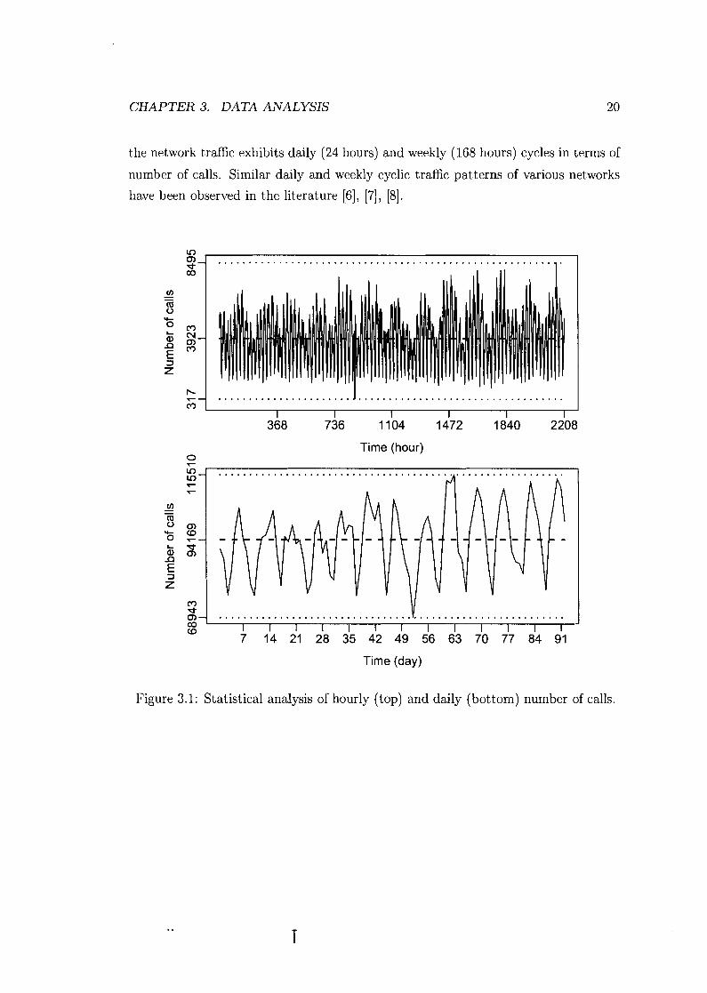
the entire network, in terms of hourly and daily number of calls, is shown in Figure 3.1.
The upper and lower dotted lines indicate the maximum and the minimum number
of calls, respectively. The middle dashed line is the mean value.
Figure 3.1 demonstrates the inherent cyclic patterns of the network traffic. We
check the periodic patterns by applying the Fast Fourier Transform (FFT) on the
network data to find t,he highest frequency in the hourly and the daily number of
calls. The FFT reveals the high frequency components at 24 for the hourly number of
calls and a t 7 for the daily number of calls, as shown in Figure 3.2. We conclude that
CHAPTER 3. DATA ANALYSIS 20
the network traffic exhibits daily (24 hours) and weekly (168 hours) cycles in terms of
number of calls. Similar daily and weekly cyclic traffic patterns of various networks
have been observed in the literature [6], [7], [8].
Time (hour)
Time (day)
Figure 3.1: Statistical analysis of hourly (top) and daily (bottom) number of calls.

CHAPTER 3. DATA ANALYSIS
Frequency (hour)
7 14
Frequency (day)
Figure 3.2: Fast Fourier Transform (FFT) analysis on hourly (top) and daily (bot- tom) number of calls. The high frequency components at 24 (top) and 7 (bottom) indicate that the network traffic exhibits daily (24 hours) and weekly (168 hours) cycles, respectively.

CHAPTER 3. DATA ANALYSIS
3.2 Analysis on agency level
Network users belong to various agencies such as RCMP, police, ambulance, and fire
department. The study of agency behavior may help network operators identify the
aggregate traffic patterns in the organizational usage of network resources. Agency
names are eliminated to protect their privacy. Instead, we use agency id to identify
the agency structure for talk groups.
The agency id in the E-Comm network ranges from 0 to 15. The agency id 0
represents unknown or corrupted agency group information of users. The network
usage statistic data of each agency is summarized in Table 3.1. The rows are sorted
in ascending order by the number of calls made by each agency. 92% of calls are made
by three agencies with id 10, 2, 5, while the remaining 13 agencies account for only
8% of the calls. The average call duration ranges from 2.3 to 5.9 seconds. We also
observed that more than 55% of calls in the network are multi-system calls. Beside
the hourly number of calls, call duration is another major factor affecting the network
resource usage. In order to measure how long and how many channels have been
occupied by a call in the network! we define the net,work resource usage for a call as:
Network resource = Call duration * Number of systems.
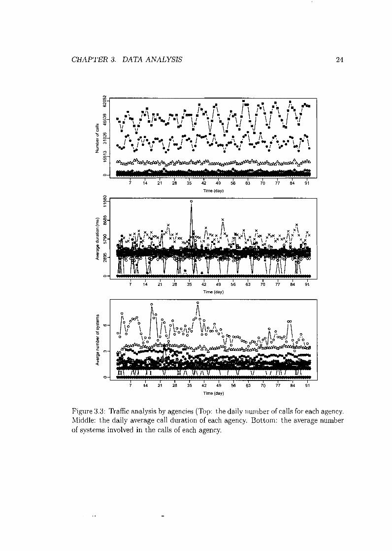
Three different aspect,s of agency traffic are shown in Figure 3.3. We use different
symbol in the figure to represent different agency. The tlop plot is the daily number
of calls for each agency. The middle plot is the daily average call duration of each
agency. The bottom plot represents the average number of systems involved in the
calls of each agency. The daily average call duration is relatively constant for agencies,
while the daily number of calls shows large variations among agencies.
3.3 Analysis on talk group level
The basic talking unit in the E-Comm network is a talk group. This is the finest
unit for our analysis. Traffic analysis on the agency level is too coarse to capture the
behavior of small talking units in the network. Even though each talk group belongs

Agency id
20 15 8 7 14 0 13 6 11 4 1 3 21 10 2 5
Sum
Number of
calls (%) 0.00% 0.00% 0.00% 0.03% 0.06% 0.11% 0.15% 0.45% 0.67% 0.95% 1.05% 1.35% 3.26% 10.97% 29.16% 51.72% 100%
Number of
calls 22 37 129
2,963 5,523 10,037 13,590 39,363 58,622 82,482 91,417 117,289 282,907 950,725
2,527,096 4,481,384 8,663,586
Number of mult i-syst em
calls
Average duration (4 2,329 2,239 4,230 4,080 3,279 3,278 5,986 3,871 3,861 3,175 3,857 4,024 3,480 3,438 3,853 3,838 3,772
4gency network usage. Table 3.1:
Number of multi-system
calls (%) 0.00% 21.62% 98.44% 20.45% 4.49% 63.44% 0.00% 3.62% 3.78% 14.38% 14.84% 33.68% 63.90% 76.02% 36.28% 71.27% 58.76%
CHAPTER 3. DATA ANALYSIS
0
7 14 21 28 35 42 49 56 63 70 77 84 91
Time (day)
0 m : -
- ln m E s - C
X
.- + m o 5 2 '0 ln
QJ 0)
f s
0
7 14 21 28 35 42 49 56 63 70 77 84 91
Time (day)
0-
I I I I 1 I I I I I I I I 7 14 21 28 35 42 49 56 63 70 77 84 91
Time (day)
Figure 3.3: Traffic analysis by agencies (Top: the daily number of calls for each agency. Middle: the daily average call duration of each agency. Bottom: the average number of systems involved in the calls of each agency.
CHAPTER 3. DATA ANALYSIS 25
to a certain agency, the organizational structure does not necessarily imply similar
usage patterns. Talk groups belonging to different agencies may have similar behavior,
while talk groups within the same agency may have dif•’ererlt behavior patterns.
A sample of talk groups' behavior patterns is shown in Table 3.2. The behavior
patterns include average resources, average duration, and average number of systems
involved in group calls. The talk groups are sorted in descending order of the total
number of calls during the 92 days. The average call duration exhibits a relatively
constant pattern with mean value of 3,621.50 ms and standard variance of 397 ms. To
the contrary, the average number of systems involved in calls is quite different. For
example, the members of talk group 1809 are usually distributed across more than 4
systems, while the members of talk group 785 often reside in one system when making
calls. Accordingly, the number of systems engaged in a call greatly affects the network
resource usage.
3.4 Summary
The preliminary st.atistica1 analysis of traffic dat,a at different levels shows the diversity
and complexity of network user's (talk group's) behavior. User's behavior exhibits
patterns that may be used to categorize talk groups. We are particularly interested
in building clusters of talk groups based on their behavior patterns. This topic is
addressed in Chapter 4.

Tal
k A
gen
cy
grou
p
id
id
801
2 81
7 2
465
5 7
85
2
1817
10
49
7 5
401
5 83
3 2
1801
10
1809
10
481
5 47
1 5
673
1
449
5 43
3 5
786
2 41
8 5
289
5 24
9 5
Nu
mb
er
of
call
s 46
1,12
8 38
2,06
5 36
3,13
8 35
4,32
4 31
2,13
1 30
3,99
1 30
3,94
8 30
3,85
4 29
4,68
7 27
8,87
2 27
8,63
4 27
6,40
4 26
0,81
3 25
8,01
9 22
6,49
2 22
5,61
2 20
7,58
3 15
9,64
9 14
5,87
5 ...
Ave
rage
A
vera
ge
Ave
rage
re
sou
rces
d
ura
tion
n
um
ber
of
use
d
bs
>
syst
ems
4,75
6.23
3,
489.
76
1.35
Table
3.2
: S
ampl
e o
f th
e r
esou
rce
consu
mptio
n fo
r va
rious
ta
lk g
roup
s.

Chapter 4
Data clustering
Data mining employs a variety of data analysis tools to discover hidden patterns and
relationships in data sets. Clustering analysis, with its various objectives, groups or
segments a collection of objects into subsets or clusters so that objects within one
cluster are more "close" to each other than objects in distinct clusters. It attempts
to find natural groups of components (or data) based on certain similarities. It is
one of the powerful tools in data mining, with applications in a variety of fields
including consumer data analysis, DNA classification, image processing, and vector
quantization.
In this Chapter, we first describe the data used for the clustering analysis. We
then introduce the Autoclass [9] tool and K-means [lo] algorithm. The results of
clustering and the comparison are also presented.
4.1 Data representing user's behavior
An object can be described by a set of measurements or by its relations to other
objects. Customers' purchasing behavior may be characterized by shopping lists with
the type and quantity of the commodities bought. Network users' behavior may be
measured as the time of calls, the average length of the call, or the number of calls
made in a certain period of time. Telecommunication companies often use call inter-
arrival time and call holding time to calculate the blocking rate and to determine the
CHAPTER 4. DATA CLUSTERING 28
network usage. In the E-Comm network, the call inter-arrival time are exponentially
distributed, while the call holding time fits a lognormal distribution [ l l ] .
The number of users' call is of particular interest to our analysis. A commonly used
metric in the telecommunication industry is the hourly number of calls. It may be
regarded as the footprint of a user's calling behavior. Units less than an hour (minute)
is large enough to capture the calling activity since a call usually lasts 3-5 seconds
in the EComm network. However, the one minute recording unit may impose large
computational cost because of the huge number of data points (92 * 24 * 60 = 132,480).
Units larger than an hour (day) are too coarse to capture user's behavior patterns
and will reduce the number of data points to merely 92 in our analysis.
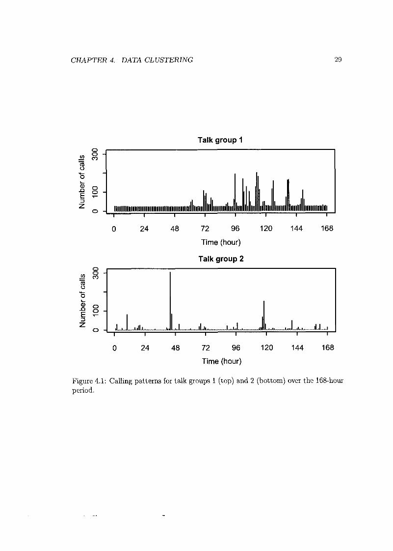
The talk group is the basic talking unit in the EComm network. Hence, we use
a talk group's hourly number of calls to capture a user's behavior. The collected 92
days of traffic data (2,208 hours) imply that each talk group's calling behavior may
be portrayed by the 2,208 ordered hourly numbers of calls. Samples of the hourly
number of calls for talk groups 1 and 2 over 168-hour are shown in Figure 4.1, while
talk group 20 and 263's calling behavior are shown in Figure 4.2. Table 4.1 shows a
small sample of the user's calling behavior. The first column shows the talk group
id. The remaining columns are the hourly number of calls starting from 2003-03-01
00:00:00 (hour 1) and ending a t 2003-05-31 23:59:59 (hour 2208). One row corresponds
to one talk group's calling behavior over the 2,208 hours. This will be used in our
clustering analysis.
For simplicity and based on prior experience with clustering tools, we selected
AutoClass [12] tool and K-means [lo] algorithms to classify the calling patterns of
talk groups.
AutoClass tool
A general approach to clustering is to view it as a density estimation problem. We
assume that in addition to the observed variables for each data point, there is a hidden,
unobserved variable indicating the "cluster membership" (cluster label). Hence, the
data are assumed to be generated from a mixture model and that the labels (cluster
CHAPTER 4. DATA CLUSTERING
Talk group I
Time (hour)
Talk group 2
0 24 48 72 96 120 144 168
Time (hour)
Figure 4.1: Calling patterns for talk groups 1 (top) and 2 (bottom) over the 168-hour period.
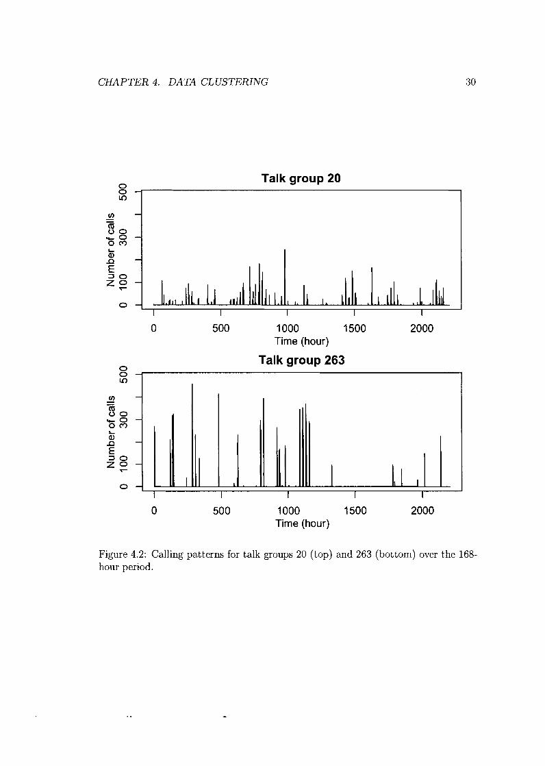
CHAPTER 4. DATA CLUSTERING
0 Talk group 20
0 V)
0 500 1000 1500 2000 Time (hour)
0 Talk group 263
0 -4 V)
V) - - - 8 o rco - 0 m L a, a - E 3 0 2 0 -
7
0 - I I I I I
0 500 1000 1500 2000 Time (hour)
Figure 4.2: Calling patterns for talk groups 20 (top) and 263 (bottom) over the 168- hour period.

CHAPTER 4. DATA CLUSTERING
Talk group id 0 1089 28 ... 113 162 230 ...
Hour 1
26 6 1 ... 3 0 3 ...
Hour 2 25 29 0 ... 0 0 0 ...
Hour 3
24 0 2 ... 0 0 3 ...
Hour 4 20 10 32 ... 5
232 77 ...
Hour 2206
30 22 13 ... 3
193 203 ...
Hour 2207
24 23 36 ... 0
176 270 ...
Hour 2208
26 0 8 1 ... 0
256 187 ...
Table 4.1: Sample of hourly number of calls for various talk groups.
identification) are hidden. In general, a mixture model M has K clusters Ci, i =
1, ..., K , assigning a probability to a data point x as:
where Wi is the mixture weight. Some clustering algorithms assume that the number
of clusters K is known a priori.
AutoClass [12] is an unsupervised classificat.ion tool based on thc classical finitme
mixture model [13]. According to Cheeseman, [9]
"The goal of Bayesian unsupervised classification is to find the most
probable set of class descriptions given the data and prior expectations."
In the past, AutoClass was applied to classify distinct user groups in Telus Mobility
Cellular Digital Packet Data (CDPD) network [8].
AutoClass was developed by Bayesian Learning Group at NASA Ames Research
Center [14]. We use AutoClass C version 3.3.4. The key features of AutoClass include:
determining the optimal number of classes automatically
handling both discrete and continuous values
handling missing values

CHAPTER 4. DATA CLUSTERING 32
"soft" probabilistic cluster membership instead of "hard" cluster membership.
AutoClass begins by creating a random classification and then manipulates it
into a high probability classification through local changes. It repeats the process
until it converges to a local maximum. It then starts over again and continues until
a maximum number of specified tries. Each effort is called a t7-y. The computed
probability is intended to cover the entire parameter space around this maximum,
rather than just the peak. Each new try begins with a certain number of clusters
and may conclude with a smaller number of clusters. In general, AutoClass begins
the process with a certain number of clusters that previous tries have indicated to be
promising.
The input data for AutoClass are stored in two files: data file (.db2) and header
file (.hd2). The data file are in vector format. The 2,208 number of calls for each talk
group are extracted from database and stored in matrix structure. Each row stands
for one talk group and each column is one of the 2,208 hourly number of calls, except
that the first column is the identification number of a talk group. In the header file,
we specify the data type, name, relative observation error for each column. Part of
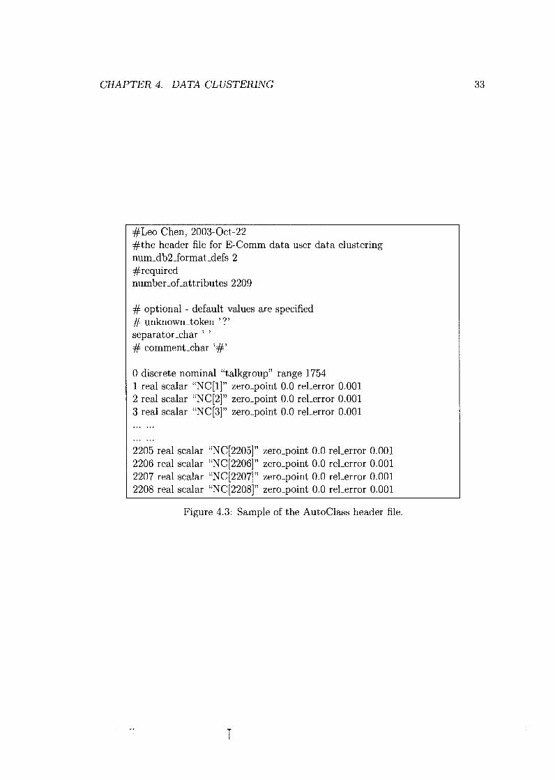
the header file is shown in Figure 4.2.
AutoClass uses a model file (.model) to describe the possible distribution model for
each attribute of the data. Four types of models are currently supported in AutoClass:
single~multinomial: models discrete attributes as multinomial distribution with
missing values. It can handle symbolic or integer attributes that are condition-
ally independent of other attributes given the class label. Missing values will be
represented by one of these existing values.
single-normal-cn: models real valued attributes as normal distribution without
missing values. The model parameters are mean and variance.
single-normal-cm: models real valued attributes as normal distribution with
missing values. The model can be applied to real scalar attributes using a
log-transform of the attributes.
CHAPTER 4. DATA CLUSTERING
#Leo Chen, 2003-Oct-22 #the header file for E-Comm data user data clustering num-db2-format-defs 2 #required number-of-attributes 2209
# optional - default values are specified # unknown-token '?' separator-char ' ' # comment-char '#'
0 discrete nominal "talkgroup" range 1754 1 real scalar "NC[l]" zero-point 0.0 rel-error 0.001 2 real scalar "NC[2Iv zero-point 0.0 rel-error 0.001 3 real scalar "NC[3In zero-point 0.0 rel-error 0.001
... ... 2205 real scalar "NC[2205]" zero-point 0.0 rel-error 0.001 2206 real scalar "NC[2206In zero-point 0.0 rel-error 0.001 2207 real scalar "NC[2207lV zero-point 0.0 rel-error 0.001 2208 real scalar "NC[2208]" zero-point 0.0 rel-error 0.001
Figure 4.3: Sample of the Autoclass header file.

CHAPTER 4. DATA CLUSTERING 34
0 multi-normal-cn: a covariant normal model without missing values. This model
applies to a set of real valued attributes, each with a constant measurement
error and without missing values, which are conditionally independent of other
attributes given the cluster label.
The model file used is given in Appendix B. A search parameters file (.sparam)
is also used to adjust the search behavior of AutoClass. The most frequently used
parameters are start-j-list, fixed-j, and max-n-tries.
0 start-jlist: AutoClass will start the search with the certain number of clusters
in the list.
0 fixed-j: AutoClass will always search for the fixed-j number of clusters, if spec-
ified.
0 maxn-tries: AutoClass stops search when it reaches the maximum number of
the tries.
The detailed description of the remaining searching and reporting parameters may be
found in the AutoClass manual [9], [15].
AutoClass used -20 hours in searching for the best clustering of the 617 talk
groups in the E-Comm data. The search results include three important values for
the clustering:
0 attribute influence values: presents the relative influence or significance of the
attributes.
0 cross-reference by case number: lists the primary class probability for each da-
tum, ordered by the case number.
0 cross-reference by class number: for each class, lists each datum in the class,
ordered by case number.
The content of one clustering report is given in Appendix B. The ten best results
of talk group clustering are summarized in Table 4.2. The number of talk groups in

CHAPTER 4. DATA CLUSTERING
Number of t r ies
653 930 940 323 542 1084 677 918 528 385
Probability
exp(-6548529.230) exp(-6592578.320) exp(-6619633.090) exp(-6622783.940) exp(-6626274.570) exp(-6637269.320) exp(-6657627.910) exp(-6658596.390) exp(-6660040.920) exp(-6671271.570)
Table 4.2: AutoClass results: 10 best clusters.
Number of clusters
24 18 21 2 4 17 24 18 19 18 12
Cluster ID Size
[3] 66 [61 23 191 20
[I21 19 [I51 18 1181 13 WI 9 PI 3
Cluster ID Size [I] 144
[41 31 PI 22
[ lo ] 20 [I31 18 1161 17 ~ 9 1 12
PI 4
Table 4.3: AutoClass results: cluster sizes.
Cluster ID Size
PI 67 PI 25 I81 21 [Ill 19 [I41 18 1171 15 POI 10
PI 3
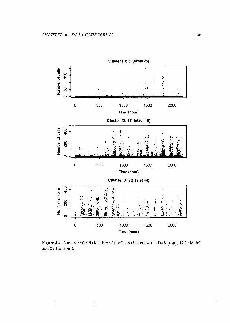
each cluster (cluster size) is also shown in the Table 4.3. Hourly number of calls for
talk groups in clusters 5, 17, and 22 are shown in Figure 4.4. Talk groups in different
clusters exhibit distinct calling behavior patterns.
4.3 K-means algorithm
K-means algorithm is one of the most commonly used data clustering algorithms. It
partitions a set of objects into K clusters so that the resulting intra-cluster similarity
is high while the inter-cluster similarity is low. The number of clusters K and the
CHAPTER 4. DATA CLUSTERING
Cluster ID: 5 (size=25)
0 500 1000 1500 2000
Time (hour)
Cluster ID: 17 (size=15)
V) - - -
s g - '5 $ - n
0 500 1000 1500 2000
Time (hour)
. -. . .I . .
Cluster ID: 22 (size=4)
5 E - . . z . . . . . ..
J.. n - I . 0 - I I I I
0 500 1000 1500 2000
Time (hour)
Figure 4.4: Number of calls for three Autoclass clusters with IDS 5 (top), 17 (middle), and 22 (bottom).

CHAPTER 4. DATA CLUSTERING 37
object similarity function are two input parameters to the K-means algorithm. Cluster
similarity is measured by the average distance from cluster objects to the mean value
of the objects in a cluster, which can be viewed as the cluster's center of gravity. The
algorithm is well-known for its simplicity and efficiency. It is relatively efficient and
stable. The use of various similarity or distance functions makes it flexible. It has
numerous variations and it is applicable in areas such as physics, biology, geographical
information system, and cosmology. However, its main drawback is its sensitivity to
the initial seeds of clusters and outliers, which may distort the distribution of data.
In addition, user sometimes may not know a priori the desired number of clusters K ,
which is the most important input parameter to the algorithm.
The distance between two points is taken as a common metric to assess the simi-
larity among the components of a population. The most popular distance measure is
the Euclidean Distance. The Euclidean distance of two data points x = (xl , 2 2 , ..., xn)
and Y = (~1,327 ..., yn) is:
We use a variation of K-means, PAM (Partitioning Around Medoids) [ lo] and our
own implementation of K-means to cluster the talk group data. The PAM algorithm
searches for K representative objects or medoids among the observations of the data
set. It finds K representative objects that minimize the sum of the dissimilarities of
the observations to their closet medoids.
We also implemented the classical K-means algorithm using the Per1 programming
language [16]. The program first seeks K random seeds as cluster centroids in the
data set. Based on the Euclidean distance of the object from the seeds, each object is
assigned to a cluster. The centroid's position is recalculated every time an object is
added to the cluster. This process continues until all the objects are grouped into the
final specified number of clusters. Objects change their cluster memberships after the
recalculation of the centroids and the re-assignment. Clusters become stable when
no object is re-assigned. Different clustering result,s are obtained depending on the
raridorn seeds. However, clustering results for different runs with the same number K

CHAPTER 4. DATA CLUSTERING 38
are relatively stable when K is not large, i.e., the clusters converge and different runs
result in almost identical cluster partitions.
Without knowing the actual cluster label for each talk group, we are unable to
measure the clustering quality using objective measurement factor, such as the F-
measure 1171. We use the inter-cluster and the intra-cluster distances to assess the
overall clustering quality. The inter-cluster distance is defined as the Euclidean dis-
tance between two cluster centroids, which reflects the dissimilarity between clusters.
The intra-cluster distance is the average distance of objects from their cluster cen-
troids, expressing the coherent similarity of data in the same cluster. A large inter-
cluster distance and a small intra-cluster distance indicate better clusters. The overall
clust,ering qualit,y indicator is defined as the difference between the minimum inter-
cluster distance and the maximum intra-cluster distance. The greater the indicator,
the better the overall clustering quality. Another measure for the clustering quality
is silhouette coefficient [lo], which is rather independent on the number of clusters,
K . Experience shows that the silhouette coefficient between 0.7 and 1.0 indicates
clustering with excellent separation between clusters.
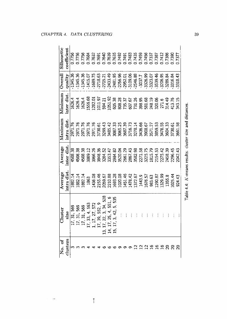
The cluster size, distance measurement, overall quality, and silhouette coefficient
of K-means clustering results for clusters with various number of K are shown in Table
4.4. Based on the overall quality and the silhouette coefficient, the best clustering
result is obtained for K = 3 (in the top three rows). Figure 4.5 shows one week
of traffic for each talk groups in the three clusters. The maximum, minimum, and
average number of calls for each cluster are also shown. The plots demonstrate the
distinct calling behavior of each cluster.
4.4 Comparison of AutoClass and K-means
To compare the clustering results of AutoClass and K-means, we enforce the number
of clusters in AutoClass by specifying the parameter f i x ed j to 3 in the search param-
eter file. The calling behavior properties for talk groups in the AutoClass clusters
and in K-means clusters are compared in Table 4.5. The three clusters identified
by K-means are more reasonable than the clusters produced by AutoClass. With
CHAPTER 4. DATA CLUSTERING
m m m m * * ? ? k t b m b m 03 0 3 m 0 3 d b 0010bhl m m m m m
m m d m ?*FV! 0 3 * 0 d b o m m * m b m m m m m

CHAPTER 4. DATA CLUSTERING
Cluster 1 (17 talk groups)
0 24 48 72 96 120 144 168
Time (hour)
Cluster 2 (31 talk groups) I
Time (hour)
Cluster 3 (569 talk groups)
Time (hour)
Figure 4.5: K-means result: number of calls in three clusters.

CHAPTER 4. DATA CLUSTERING
Table 4.5: Comparison of talk group calling properties (AC: AutoClass, K: K-means, nc: number of calls).
Alg.
K-means clustering, the first cluster has 17 talk groups, representing the busiest dis-
patch groups whose main tasks are coordinating and scheduling other talk groups
for certain tasks. The second cluster contains 31 talk groups with medium network
usage. The last, cluster ident,ifies a group of least frequent network users who made on
average no more than 16 calls per hour. These interpretations of clusters have been
confirmed by domain experts. On the contrary, it is difficult to provide reasonable
explanations for group behavior for the three clusters identified by AutoClass. Thus,
we use the three clusters identified by K-means in the prediction of network traffic.
4.5 Summary
Clu. size
Clustering analysis of the talk groups' calling behavior reveals hidden structure of
talk groups by grouping the talk groups with similar calling behavior rather than by
their organizational structure.
We used AutoClass tool and applied K-means algorithm to identify clusters of
talk groups based on their calling behavior. Talk groups' behavior patterns are then
categorized and extracted from the clusters. The optimal number of clusters is diffi-
cult to determine. By comparing the overall quality measurement and the silhouette
coefficient measure, we found that three is the best number of clusters for K-means
algorithm. Based on the domain knowledge, the three clusters identified by K-means
Min. Max. Avg. nc nc n c
Total Total nc nc (%)

CHAPTER 4. DATA CLUSTERING 42
are more reasonable than clusters produced by Autoclass. Other clustering algo-
rithms, such as hierarchical [18] and density based [19] clustering may also be used to
cluster the user data.

Chapter 5
Data prediction
In this Chapter, we describe the time series data analysis and the Auto-Regressive
Integrated Moving Average (ARIMA) models. We describe how to identify, esti-
mate, and forecast network traffic using the ARIMA model. We also present the
cluster-based prediction models and compare the prediction results with the results
of traditional prediction based on aggregate traffic.
5.1 Time series data analysis
Performance evaluation techniques are important in the design of networks, services,
and applications. Of particular interest are techniques employed to predict the QoS
related network performance. Modeling and predicting network traffic are essential
steps in performance evaluation. It helps network planners understand the underlying
network traffic process and to predict future traffic. Analysis of commercial network
traffic is difficult because the commercial network traffic traces are not easily available.
Furthermore, there are privacy and business issues to consider.
The Erlang-C model [20], currently used by the E-Comm staff, was developed
based on individual user's calling behavior in wired networks. It considers no-group
call behavior in t,runked radio systems. Network traffic may also be considered as
a series of observations of a random process, and, hence, the classical time-series
prediction ARIMA models can be used for traffic prediction.

CHAPTER 5. DATA PREDICTION 44
We employ the Seasonal Autoregressive Integrated Moving Average (SARIMA)
model [21], a special case of ARIMA, to predict the EComm network traffic. SARIMA
models have been applied to modeling and predicting traffic from both large scale
networks (NSFNET [22]) and from small scale sub-networks [23]. The fitted model
is only an approximation of the data and the quality of the model depends on the
complexity of the phenomenon being modeled and the understanding of data.
ARIMA model
The ARIMA model, developed by Box and Jenkins in 1976 [21], provides a systematic
approach to the analysis of time series data. It is a general model for forecasting a
time series that can be stationarized by transformations such as differencing and log
transformation. Lags of the differenced series appearing in the forecasting equation
are called auto-regressive terms. Lags of the forecast errors are called moving average
terms. A t,ime series that needs to be differenced to be made stationary is said to be
an integrated version of a stationary series. Random-walk and random-trend models,
autoregressive models, and exponential smoothing models (exponential weighted mov-
ing averages) are special cases of the ARIMA models [24]. ARIMA model is popular
because of its power and flexibility.
5.2.1 Aut oregressive (AR) models
Regression model is a widely applied multivariate model used to predict the target
data based on observations and to analyze the relationship between observations and
predictions. Autoregressive model is conceptually similar to the regression model. In-
stead of the multi-variative observed data, the previous observations of the univariate
target data are used as the effective factors of the target dat,a. The regression model
assumes the future value of the target variable to be determined by other related
observed data, while the autoregressive model assumes the future value of the target
variable to be determined by the previous value of the same variable. An AR model
closely resembles the traditional regression model.
CHAPTER 5. DATA PREDICTION
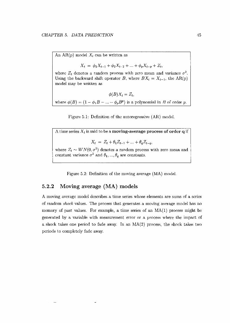
An AR(p) model Xt can be written as
Xt = 41Xt-1 + 42Xt-2 + ... + 4pXt-p + Zt,
where Zt denotes a random process with zero mean and variance a2. Using the backward shift operator B, where BXt = XtPl, the AR(p) model may be written as
4 ( W t = Zt,
where 4(B) = (1 - d l B - ... - 4,Bp) is a polynomial in B of order p.
Figure 5.1 : Definition of the autoregressive (AR) model.
A time series Xt is said to be a moving-average process of order q if
Xt = Zt + 01Zt-1 + ... + 0,Zt-,,
where Zt -- W N ( 0 , a2) denotes a random process with zero mean and constant variance a2 and 01, ..., 0, are constants.
Figure 5.2: Definition of the moving average (MA) model.
5.2.2 Moving average (MA) models
A moving average model describes a time series whose elements are sums of a series
of random shock values. The process that generates a moving average model has no
memory of past values. For example, a time series of an MA(1) process might be
generated by a variable with measurement error or a process where the impact of
a shock takes one period to fade away. In an MA(2) process, the shock takes two
periods to completely fade away.

CHAPTER 5. DATA PREDICTION
An ARIMA(p, d, q) model Xt can be written as
where q5(B) and O(B) are polynomials in B of finite order p and q, respectively. The backward shift operator B is defined as BiXt = XtPi. A SARIMA (p, d, q) x (P, D, Q)s model exhibits seasonal pattern and can be represented as:
where q5(B) and 8(B) represent the AR and MA parts, and q5(Bs) and 8(BS) represent the seasonal AR and seasonal MA parts, respectively. B is the back-shift operator BiXt = XtPi.
Figure 5.3: Definition of the AR.IMA/SARIMA model.
5.2.3 SARIMA ( p , d , q ) x ( P , D , Q ) s models
The ARIMA model includes both autoregressive and moving average parameters and
explicitly iricludes in the forrnulatiori of t,he model differericing, which is used to sta-
tionarize the series. The three types of parameters in the model are: the autoregressive
order (p), the number of differencing passes (d), and the moving average order (q).
Box and Jenkins denote it as ARIMA (p, d , q) [21]. For example, a model ARIMA (0,
1, 2) means that it contains 0 (zero) autoregressive (p) order, 2 moving average (q)
parameters, and the model fits the series after being differenced once (1). A SARIMA
model is a ARIMA model plus seasonal fluctuation. It comprises normal orders (p,
d , q) and seasonal orders (P, D, Q), and the seasonal period S. A general SARIMA
model is denoted as SARIMA (p, d, q) x (P, D, Q)s.

CHAPTER 5. DATA PREDICTION
5.2.4 SARIMA model selection
The general ARIMA model building process has three major steps:
model identification
model estimation
model ~erificat~ion.
Model identification is used to decide the orders of t,he model, i.e., to determine the
value of orders p, d, q, seasonal orders P, D, Q, and the seasonal period S. The 4(x)
and 6(x) coefficients are computed in the model estimation phase, using minimum
linear square error method or maximum likelihood estimation methods. Models are
verified by diagnostic checking on the null hypothesis of the residual or by various
tests, such as Box-Ljung and Box-Pierce tests [21], [24], [25].
The major tools used in the model identification phase include plots of the time
series, correlograms of autocorrelation function (ACF), and partial autocorrelation
function (PACF). Model identification is often difficult and in less typical cases re-
quires not only experience but also a good deal of experimentation with models with
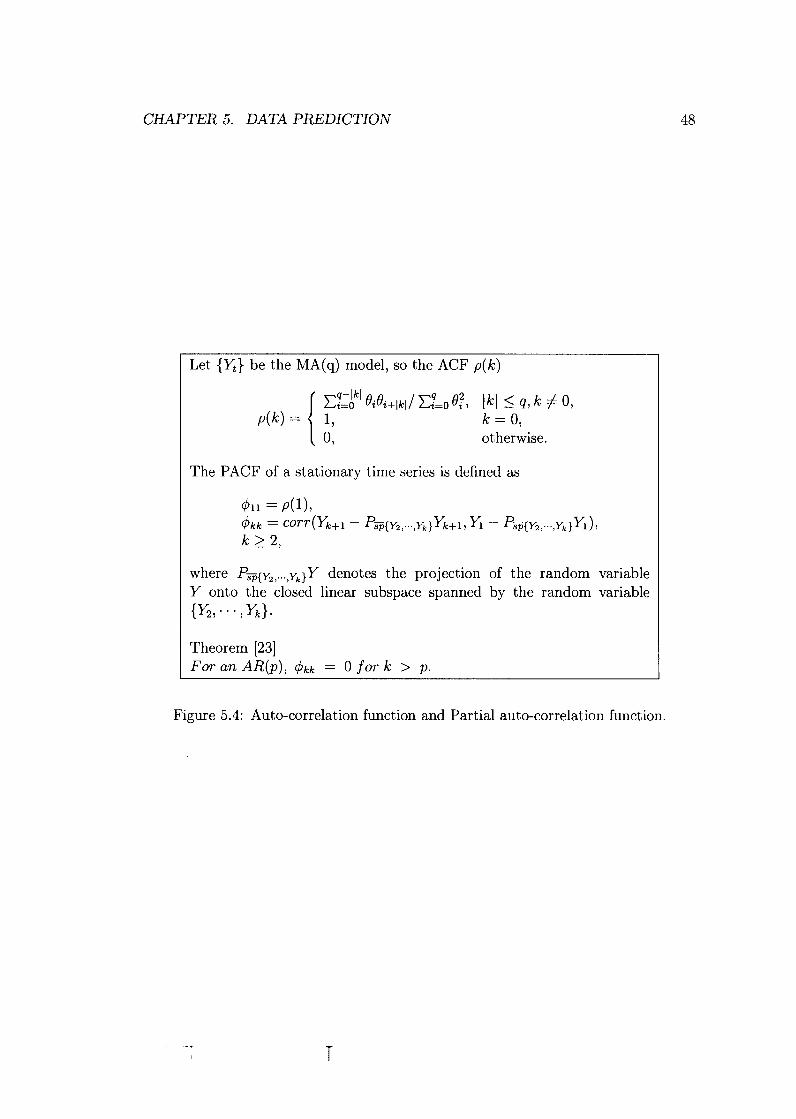
various orders and parameters. The relation of the ACF with the MA(q) model, and
the relation of the PACF with the AR(p) model, are shown in Figure 5.4.
We use three measurements to find the best models and check the validity of the
model parameters. A smaller value of the measurement indicates a better selection of
model.
Akaike's Information Criterion (AIC)
AIC = -2ln(max.likelihood) + 2p
Akaike's Information Criterion Corrected (AICc)
AICc = AIC + 2(p + l ) (p + 2)/(N - p - 2)
Bayesian Information Criterion (BIC)
B I C = -2ln(max.likelihood) + p + plnN
CHAPTER 5. DATA PREDICTION
I Let {Y,} be the MA(q) model, so the ACF p(k)
I The PACF of a stationary time series is defined as
where Pg{Y2,...,Yk}Y denotes the projection of the random variable Y onto the closed linear subspace spanned by the random variable {Y27. . . , Yk}.
Theorem 1231 For an AR(p), q5kk = 0 for k > p.
Figure 5.4: Auto-correlation function and Partial auto-correlation function.
CHAPTER 5. DATA PREDICTION
nmse 0.173 0.379 0.174 0.175
0.5253 0.411 0.546 0.537 0.404
AIC 20558.7 22744.6 23129.8 23145.1 25292.1 25332.6 25345.9 25360.5 25361.2
BIC 20590.3 22826.8 23161.9 23170.8 25382.1 25371.2 25429.4 25392.6 25399.7
Table 5.1: Summary of SARIMA models fitting measurement.
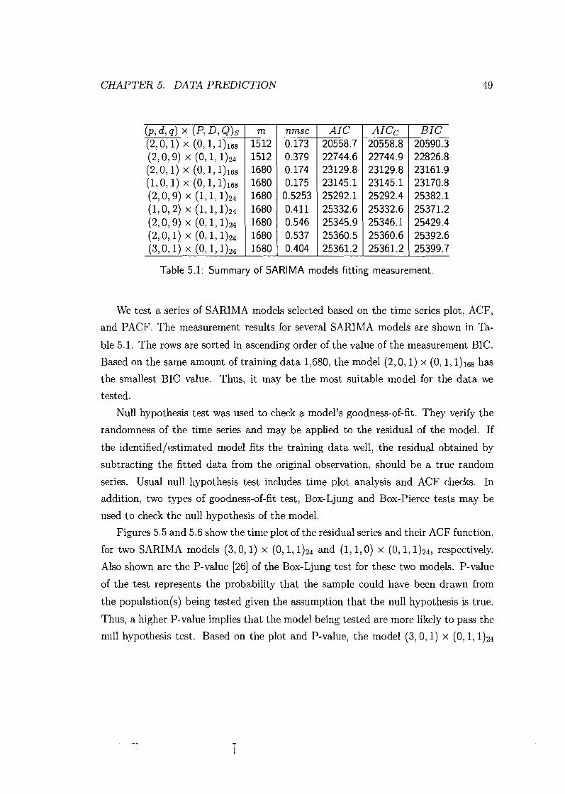
We test a series of SARIMA models selected based on the time series plot, ACF,
and PACF. The measurement results for several SARIMA models are shown in Ta-
ble 5.1. The rows are sorted in ascending order of the value of the measurement BIC.
Based on the same amount of training data 1,680, the model (2,0,1) x (O,1, has
the smallest BIC value. Thus, it may be the most suitable model for the data we
tested.
Null hypothesis test was used to check a model's goodness-of-fit. They verify the
randomness of the time series and may be applied to the residual of the model. If
the ideritified/estimated model fits the training data well, the residual obtained by
subtracting the fitted dat,a from the original observation. should be a true random
series. Usual null hypothesis test includes time plot analysis and ACF checks. In
addition, two types of goodness-of-fit test, Box-Ljung and Box-Pierce tests may be
used to check the null hypothesis of the model.
Figures 5.5 and 5.6 show the time plot of the residual series and their ACF function,
for two SARIMA models (3 ,0 , l ) x ( O , 1 , and (1,1,O) x ( O , 1 , respectively.
Also shown are the P-value 1261 of the Box-Ljung test for these two models. P-value
of the test represents the probability that the sample could have been drawn from
the population(s) being tested given the assumption that the null hypothesis is true.
Thus, a higher P-value implies that the model being tested are more likely to pass the
null hypothesis test. Based on the plot and P-value, the model (3,0,1) x ( O , 1 ,

CHAPTER 5. DATA PREDICTION
passed the null hypothesis test, while the model (1,1,O) x ( O , 1 , failed.
5.3 Prediction based on aggregate traffic
The correlograms of the autocorrelation function and the partial autocorrelation func-
tion of the E-Comm data are shown in Figures 5.7 and 5.8, respectively. By differ-
encing the sample data with 24 hours lag, we estimate from the ACF shown in Figure
5.7 that the MA order could be up to 9. Based on the PACF shown in Figure 5.8,
we estimate that the order of AR part is 2 because of the apparent cut-off at lag 2.
Hence, the ARIMA models (2, 0, 1) and (2, 0, 9) are selected as model candidates.
The order (0, 1, 1) are commonly used for seasonal part (P, Dl Q). It is selected
because the cyclical seasonal pattern itself is usually a random-walk process and may
be modeled as an MA (1) process after one time differencing. Thus, we use the order
of (0, 1, 1) for seasonal pattern.
A useful metric called normalized mean square error (nmse) is used to measure the
prediction quality by comparing the deviation of the predicted data and the observed
data. The nmse of the forecast is equal to the normalized sum of the variance of the
forecast divided by the squared bias of the forecast. It is defined as
where ai is the observed data, bi is the prediction, and Si is the mean value of ai.
Smaller values of nmse indicate better model performance.
An open source statistical tools R [27], [28], [29] was used to identify, estimate, and
verify the SARIMA model and to forecast the traffic. The E-Comm network traffic
possesses both daily and weekly patterns. Hence, both 24-hour and 168-hour (one
week) intervals are selected as seasonal period parameters. Hence, in addition to the
(2,0,9) x (O,1, and (2,0,1) x (O,1, models, two models (2,0,9) x (0,1,
and (2,0,1) x ( O , 1 , are also used to predict the network traffic. The four models
and corresponding parameters fitted for the E-Comm network traffic are shown in
Table 5.2. The model performance is tested with four groups of data (A, B, C, and

CHAPTER 5. DATA PREDICTION
Standardized Residuals
Time
p values for Ljung-Box statistic
Figure 5.5: Residual analysis: diagnostic test for model (3,0,1) x ( O , l ,

CHAPTER 5. DATA PREDICTION
Standardized Residuals
Time
ACF of Residuals
p values for Ljung-Box statistic
Figure 5.6: Residual analysis: diagnostic test for model ( 1 , 1 , O ) x ( O , l ,

CHAPTER 5. DATA PREDICTION
S'O TO- 33v
Figure 5.7: Number of calls: sample auto-correlation function (ACF).

CHAPTER 5. DATA PREDICTION
0 rn
V) CV
0 CV
0) (I] J
V) 7
0 7
V)
0
0 rn
V) CV
0 CV
0) (I] J
V) 7
0 7
V)
0
0 rn
V) CV
0 CV
0) (I] J
V) 7
0 7
V)
0
Figure 5.8: Number of calls: sample Partial auto-correlation function (PACF).

CHAPTER 5. DATA PREDICTION
No. A 1 A2 A3 A4 B 1 B2 B3 B3 C1 C2 C3 C4 D l D2 D3 D4
Trained (m) 1512 1512 1512 1512 1680 1680 1680 1680 1920 1920 1920 1920 2016 2016 2016 2016
Predicted (n) 672 672 672 672 168 168 168 168
nmse 0.3790 0.3803 0.1742 0.1732 0.3790 0.4079 0.1736 0.1745 0.3164 0.1941 0.1002 0.0969 0.3384 0.3433 0.1282 0.1178
Table 5.2: Aggregate-traffic-based prediction results.
D). We forecast the future n traffic data based 011 m past traffic data samples. In
Table 5.2, p , d , q represent the order of the AR. difference, and MA model for the
original data points, respectively. The P, D, Q represent the order of AR, difference,
and MA model for the seasonal pattern, respectively. S is the seasonal period for the
models.
Four SARIMA models with four groups of training data are shown in Table 5.2.
The models differ in the order of moving average and the seasonal period.
Model 1: (2 ,0,9) x (0,1,1)24 (rows A l l B1, C1, and D l ) is the model with
24-hour seasonal period and moving average of order 9. The model performance
does not depend on the number of training data, with nmse ranging from 0.3164
to 0.3790.
Model 2: (2 ,0,1) x (0,1,1)24 (rows A2, B2, C2, and D2) is the model with
24-hour seasonal period and moving average of order 1. It exhibits similar

CHAPTER 5. DATA PREDICTION 56
prediction effectiveness as Model 1. It performs bett'er in row C2 than model 1
in row C1.
Model 3: (2,0,9) x (O,1, (TOWS A3, B3, C3, and D3) is the model with
a 168-hour period weekly cycle. It differs from Model 1 only in the seasonal
period, but provides much better prediction results than Model 1.
Model 4: (2 ,0,1) x ( O , 1 , 1)16S (rows A4, B4, C4, and D4), differs from Model 2
in the seasonal period. It performs better than Model 2.
The comparisons of rows A1 with A2, B1 with B2, and D l with D2, indicate that
Model 1 leads to better prediction results than Model 2. However, the prediction C1 is
worse than C2. Furthermore, for all four groups of training data, Models 3 and 4 with
168-hour period always lead to better prediction results than Models 1 and 2 with 24-
hour period. The 24-hour period models assume that the traffic is relatively constant
for a weekday, while the 168-hour period models take into account traffic variations
between between weekdays. To predict traffic on a Wednesday based on Tuesday's
data not as accurate as predicting Wednesday's traffic based on the data of previous
Wednesdays. However, the computational cost of identifying and forecasting 168-hour
period models is much larger that for the 24-hour period models. Often, 168-hour
models require over 100 times the CPU needed for 24-hour models. A comparison
of the prediction results of the 24-hour model and the 168-hour model in predicting
one future week of traffic based on the 1,680 past hours is shown in Figure 5.9. It
is consistent with the nmse value. The 168-hour period model performs better than
the 24-hour period model. The continuous curve shows the observation data. Symbol
"0" indicate the predicted traffic based on the 168-hour season model. Symbol "*" denotes the prediction of the 24-hour season model. Based on the nmse values, the
prediction of the 168-hour based model fits better the observations than the prediction
based on the 24-hour model.
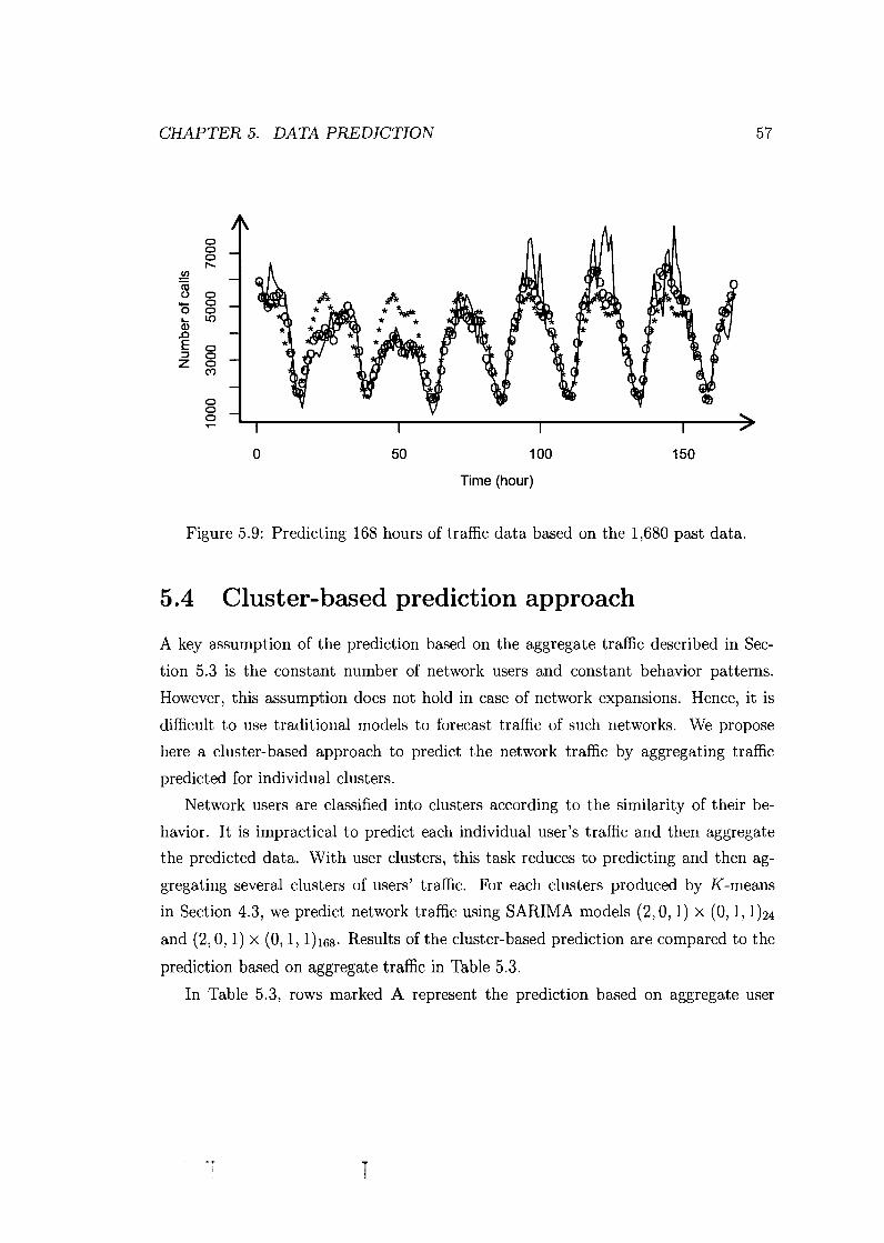
CHAPTER 5. DATA PREDICTION
50 100
Time (hour)
Figure 5.9: Predicting 168 hours of traffic data based on the 1,680 past data.
5.4 Cluster-based prediction approach
A key assumption of the prediction based on the aggregate traffic described in Sec-
tion 5.3 is the constant number of network users and constant behavior patterns.
However, this assumption does not hold in case of network expansions. Hence, it is
difficult t>o use traditional models to forecast traffic of such networks. We propose
here a cluster-based approach to predict t,he network traffic by aggregating traffic
predicted for individual clusters.
Network users are classified into clusters according to the similarity of their be-
havior. It is impractical to predict each individual user's traffic and then aggregate
the predicted data. With user clusters, this task reduces to predicting and then ag-
gregating several clusters of users' traffic. For each clusters produced by K-means
in Section 4.3, we predict network traffic using SARIMA models (2,0,1) x ( O , 1 ,
and (2,0,1) x (O,1, l)lss. Results of the cluster-based prediction are compared to the
prediction based on aggregate traffic in Table 5.3.
In Table 5.3, rows marked A represent the prediction based on aggregate user

CHAPTER 5. DATA PREDICTION
Table 5.3: Summary o f t he results o f cluster-based prediction.
Cluster 1
nmse 1.1954
( ~ , d , q ) (P,D,Q) (2,0,1) ( 0 1 )
S m n 24 1680 48

CHAPTER 5. DATA PREDICTION 59
traffic (without clustering of users) using the model shown in rows A2, B2, C2, and
D2 in Table 5.2. Rows 1, 2, and 3 represent traffic prediction for user clusters 1, 2, and
3, respectively. Row * is the weighted aggregate prediction of network traffic based
on the prediction for three user clusters. Row 0 stands for the optimized weighted
aggregate prediction. Note that the nmse > 1.0 for clusters 1 and 2 implies that the
prediction results are worse than prediction based on the mean value of past data. A
better prediction shown in row 0 is obtained if the mean value prediction is adopted
for clusters 1 and 2. We named it the optimized cluster-based prediction. Even with
un-optimized clustered based prediction (row *), the prediction results are not worse
than results of prediction based on aggregate traffic (rows A).
The advantage of the cluster-based prediction is that we could predict traffic in
a network with variable number of users as long as the new user groups could be
classified into the existing user clusters. The computational cost of forecasting the
network traffic is reduced to the number of clusters times the prediction cost for one
cluster.
5.5 Additional prediction results
Additional prediction results are presented in Tables 5.4 - 5.7. The experimental
results show that 57% of the cluster-based prediction models perform better than the
prediction models based on aggregate traffic when the seasonal period is 168 hours.
Furthermore, 7 out of 8 optimized models give better prediction results when the
model seasonal period is 24 hours.
5.5.1 Comparison of predictions with the (2 ,0 ,1 ) x (0, 1,
model
The results of cluster-based prediction and the prediction based on aggregat.e traffic
are compared in Tables 5.4 and 5.5. In the tables, pdq, PDQ, and S are SARIMA
model orders, seasonal orders, and season period, respectively. m is the number of
model training data and n is the number of predicted data. Tables 5.4 and 5.5 also

CHAPTER 5. DATA PREDICTION 60
show the nmse for prediction of each cluster, nmse for prediction based on aggregate
user traffic, nmse for cluster-based prediction, and nmse for optimized cluster-based
prediction, if any. Note that we use the same optimization method as used in Table 5.3:
we use the mean value of training data m to replace the "bad" cluster predictions when
nmse > 1.0. Rows marked "()" indicate that the cluster-based predictions perform
better than the predictions based on aggregate traffic (8 out of 56). Rows marked "[I" show that the optimized cluster-based prediction performs better than the prediction
based on aggregate traffic (7 out of 56). 7 out of 8 optimized predictions perform
better than the aggregate-traffic-based predictions, which proves the effectiveness of
the proposed optimization method.
5.5.2 Comparison of predictions with the (2,0,1) x (O,l,
model
The results of cluster-based prediction and the prediction based on aggregat,e traffic
using SARIMA model (2,0,1) x ( O , 1 , are compared in Tables 5.6 and 5.7. In
the tables, pdq, PDQ, and S are SARIMA model orders, seasonal orders, and season
period, respectively. m is the number of model training data and n is the number of
data predicted. Tables 5.6 and 5.7 also show the nmse for prediction of each cluster,
nmse for predi~t~ion based on aggregat,e user traffic, nmse for cluster-based prediction,
and nmse for optimized cluster-based prediction, if any. Note that we also applied
the same optimization method as used in Table 5.3, which replaces "bad" prediction
results (nmse > 1.0) with the mean value of training data m. None of the optimized
cluster-based predictions performs better than the predictions based on aggregate user
traffic. However, more t.han 57% cluster-based predictions perform better than the
predictions based on aggregate traffic, which are shown in rows marked "0".
5.6 Summary
In this Chapter, we described the analysis of time series data, emphasizing the
SARIMA models. The SARIMA rnodel was used to fit the aggregate network traffic

nmse nmse nmse cluster1 cluster2 cluster3 0.3237 0.5481 0.3084
nmse aggregate
0.2546 0.3431 0.3708 0.3559 0.3904 0.3905 0.3806 0.1203 0.1661 0.3206 0.3673 0.3422 0.3122 0.3016 0.221
0.2894 0.3255 0.3103 0.3081 0.334
0.4105 0.08545 0.09983 0.2409 0.3387 0.3703 0.3469 0.3378
nmse clusters ( 0.2416 ) ( 0.3324 ) ( 0.3605 ) ( 0.3456 ) ( 0.381 ) ( 0.3831 ) ( 0.3748 ) ( 0.1187 )
0.167 0.3419 0.3933 0.3633 0.3223 0.3046 0.2535 0.2986 0.3321 0.3151 0.3107 0.3352 0.4117 0.09052
0.103 0.2449 0.3429 0.3738 0.3504 0.3414
Table 5.4: Comparison of predictions with (2,0,1) x (O,1, model: part 1.
nmse optimized
n/a n/a n/a n/a n/a n/a n /a n/a n/a n/a n/a n/a n/a n /a
0.2993
n/a n/a n/a n/a n/a n/a n/a n/a n/a n/a n/a n/a n /a
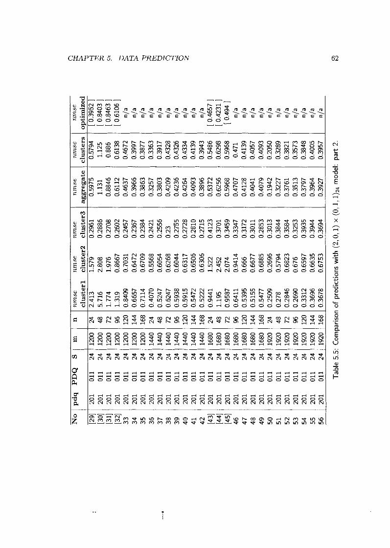
nm
se
nm
se
nm
se
clu
ster
1
clu
ster
2
clu
ster
3
2.41
3 1.
579
0.29
61
nm
se
aggre
gate
0.
5975
1.
131
0.88
46
0.61
12
0.46
37
0.39
66
0.38
63
0.32
57
0.38
03
0.42
09
0.42
36
0.42
64
0.40
93
0.38
96
0.53
72
0.62
56
0.59
68
0.47
07
0.41
28
0.40
41
0.40
79
0.19
42
0.32
27
0.37
61
0.35
13
0.37
97
0.39
64
0.39
27
nm
se
clu
ster
s 0.
5794
1.
125
0.88
6 0.
6138
0.
4672
0.
3997
0.
3877
0.
3363
0.
3917
0.
4328
0.
4326
0.
4334
0.
4139
0.
3943
0.
5486
0.
6298
0.
5968
0.
471
0.41
39
0.40
57
0.40
93
0.20
50
0.32
89
0.38
21
0.35
73
0.38
48
0.40
05
0.39
57
Tab
le 5
.5:
Com
paris
on o
f pr
edic
tions
wit
h (
2,0
,1)
x (O
,1,
mod
el:
part
2.

CHAPTER 5. DATA PREDICTION
lm I m m m m m m m m m m m m m m m m m m m m m m m m m m m w w w w w w w w w w w w w w w w w w w w w w w w w w w d d d d d d d d d d d d d d d d d d d d d d d d d d d
nnnnnnnnn n n n n 0 d rU P7 e U, W b 03 W b ~ O d d d d d d d d d ~ o d N ~ ~ m w b

Ta
ble
5.7
:
nm
se
nm
se
nm
se
clu
ster
1 cl
ust
er2
clu
ster
3
0.98
96
0.51
87
0.17
94
nm
se
aggr
egat
e 0.
1357
0.
1537
0.
1552
0.
1515
0.
1512
0.
1531
0.
1794
0.
1802
0.
1859
0.
2106
0.
2078
0.
1910
0.
1742
0.
1527
0.
1597
0.
1633
0.
1739
0.
1808
0.
1321
0.
1149
0.
1068
0.
1094
0.
1236
0.
1627
0.
1745
0.
1809
0.
1645
nm
se
clu
ster
s (
0.12
26 )
(
0.14
91 )
(
0.15
27 )
(
0.14
98 )
(
0.14
95 )
(
0.15
12 )
(
0.17
72 )
(
0.17
84 )
(
0.18
49 )
0.
2196
0.
2094
(
0.19
09 )
( 0.
1729
)
( 0.
151
) (
0.15
60 )
(
0.15
89 )
(
0.17
16 )
(
0.17
80 )
(
0.12
98 )
0.
1168
0.
1086
0.
1100
0.
1238
0.
1630
0.
1750
(
0.18
05 )
0.
1654
Com
paris
on o
f pre
dic
tions
wit
h (
2,0
,1) x
(O
,l,
mo
de
l: p
art
2
0
nm
se
opti
miz
ed
E 'n
n/a
2 n/
a 'a
n/a
9

CHAPTER 5. DATA PREDICTION 65
data and the traffic of user clusters. We compared the prediction based on aggre-
gate traffic with cluster-based prediction. Based on our tests, we noted that 57% of
the cluster-based prediction performed better than the aggregat,e t,rafic prediction
with SARIMA model (2 ,0 ,1) x (O,1, With SARIMA model (2 ,0 ,1) x (O,1,
cluster-based prediction performs better than prediction based on aggregate traffic in
8 out of 56 tests and 7 optimized cluster-based predictions gave better results too.
The advantage of clu~t~er-based traffic prediction is the flexibility of predicting variable
number of users and the reduction of the computational cost.

Chapter 6
Conclusion
In this thesis, we proposed a new prediction approach by combining clustering tech-
niques with traditional time series prediction modeling. The new approach has been
tested to predict the network traffic from an operational trunked radio system. We an-
alyzed the network traffic data arid extracted useful data from the E-Comm network.
We explored the effectiveness and usefulness of clustering techniques by applying
Autoclass tool and K-means algorithm to classify network talk groups into various
clusters based on the users' behavior patterns. To solve the computational cost prob-
lem of "bottom-up" approach and the inflexibleness problem of "top-down" approach,
we proposed a cluster-based traffic prediction method. We applied the cluster-based
SARIMA models and aggregate-traffic-based models to predict the network traffic.
The cluster-based prediction method produced comparable prediction results as the
prediction based on aggregate network traffic. In our t,ests with the 168-hour SARIMA
model, the cluster-based prediction performs better than the aggregate-traffic-based
prediction. With the 24-hour SARIMA model, cluster-based predictions (8 out of
56 tests) and optimized cluster-based prediction (7 out of 56 tests) perform better
the aggregate-traffic-based predicbions. Furt,hermore, the cluster-based prediction a p
proach is applicable to networks with variable number of users where the prediction
based on aggregate-traffic-based could not be applied. Utilizing the network user
clusters indicates a possible prediction approach for operational networks. Our ap-
proach may also enable network operators to predict network traffic and may provide

CHAPTER 6. CONCLUSION 6 7
guidance for future network expansion. Another contribution of this research project
is the illustration how data mining techniques may be used to help solve practical
real-world problems.
We developed database processing and analysis skills while dealing with the 6
Gbyte database. By applying unsupervised classification method on the traffic data,
we learned that it is rarely possible to produce useful results without having the
domain knowledge. The discovery of important clusters is a process of finding classes,
interpreting the results, transforming and/or augmenting the data, and repeating the
cycle. The cluster-based prediction model illustrates the application of clustering
techniques to traditional network traffic analysis.
6.1 Related and future work
Prior analysis of traffic from a metropolitan-area wireless network and a local-area
wireless network indicated the recurring daily user behavior and mobility patterns [6],
171. Analysis of billing records from a CDPD mobile wireless network also revealed
daily and weekly cyclic patterns [8]. The analysis of traffic from a trunked radio net-
work traffic showed that the call holding time distribution is approximately lognormal,
while the call inter-arrival time is close to an exponential distribution [ l l ] . Channel
utilization and the multi-system call behavior of trunked radio network have been
also simulated using OPNET [30] and a customized simulation tool (WarnSim) [31].
We also experimented with a Bayesian network based approach to explore the
causal and conditional relationships among the different characteristics of user behav-
ior, such as call duration, number of systems in a call, caller id, and callee id. We
used B-course 1321, 1331 and Tetrad 1341, 1351 and constructed Bayesian network from
the user calling behavior data. Analysis results are presented in Appendix C.
Since we orily have three months of traffic data, we were able to extract only
the daily and weekly patterns of the user calling behavior. A larger volume of data
may enable identifying the monthly behavior patterns. Traffic models could also be
compared using simulation tools. This would help verify the prediction results.

Appendix A
Data table, SQL, and R scripts
A.1 Call-Type table
Call-type
Group call
Individual call
Emergency call
System call
Morse code
Test
Paging
Scramble
Group set
System log
Start emergency
Cancel emergency
N/A

APPENDIX A. DATA TABLE, SQL, AND R SCRIPTS
A.2 SQL scripts for statistical output
Script to compute the average resource consumption for each talk group, in descending
order of the number of calls during the 92 days.
SELECT callee, agency, sum(n-calls) AS sn,
TRUNCATE( SUM( n-calls * avgRes ) / SUM( n-calls 1, 2 ) AS aR,
TRUNCATE( SUM( n-calls * avgDur ) / SUM( n-calls 1, 2 ) AS aD,
TRUNCATE( SUM( avgSys * n-calls ) / SUM( n-calls ) , 2 ) AS aSys
INTO OUTFILE '/tmp/dump/tg.res.stat3 FROM tgStat
GROUP BY callee ORDER BY sn desc;
A.3 R scripts for prediction test and result sum-
mary
A.3.1 R script for prediction test
pred.test.24~-function(data, p=2, d=O, q=l, P=O, D=l, Q=l,
start=240, end=1920, step=240, p.start=24, p.end=168, p.step=24, prefix)
C result<-list () ;
counter<-0 ;
for (m in seq(start, end, step))
C mm<-as . integer (m) ; worked<-0;
for (n in seq(p. start, p. end, p. step))
C f.name<-paste(prefix, "predl',mm,n,"(",p,d,q,P,D,Q,")-24",sep="-");
cat (counter, " : checking file" , f .name) ;
if (file.exists(paste("./pred.test.24/", f.name, sep=""))) C cat ( " . . . . . . tested already\nM) ;

APPENDIX A. DATA TABLE, SQL, AND R SCRIPTS
worked<-I;
if (file.info(paste("./pred.test.24/", f.name, sep=""))$size != 0) (
load(paste(" . /pred. test. 24/" ,f .name, sep="")) ; x.arima<-result$arima;
x.a.t<-result$m.t;
break;
3 3
1 if (worked == 0) (
cat ("building model based on", mm, "data! \ntt) ;
counter<-counter+l;
cat (counter, " :predictt' ,n, "based on" ,mm, "data !\nu) ;
f.name<-paste(prefix, "pred",mm,n,"(",p,d,q,P,D,Q,")-24",sep="-");
if (file . exists (paste (I1. /pred. test. 24/11, f .name, sep=" " ) ) ) (
cat ("tested already\nl') ;
next ;
1 x.p.t<-system.time(x.pred<-predict(x.arima, n.ahead=n));
x.nmse<-nmse(x.pred$pred[l:n] , data[(mm+l): (mm+n)l);
cat("nmse=",x.nmse, "for ( " ,p ,d,q,P,D,Q,")-24\n1I) ;
result. predc-x. pred$pred [I : nl ;
result<-list(par=c(p,d,q,P,D,Q,24,mm,n), arima=x.arima,

APPENDIX A. DATA TABLE, SQL, AND R SCRIPTS
pred.test.l68<-function(data, p=2, d=O, q=l, P=O, D=l, Q=1,
start=840, end=1680, step=l68, p. start=24, p. end=l68, p. step=24, prefix)
x result<-list 0 ;
counter<-0;
for (m in seq(start, end, step))
x mm<-as.integer(m);
worked<-0;
for (n in seq(p.start, p.end, p.step))
x f.name<-paste(prefix, "pred",mm,n,"(",p,d,q,P,D,Q,")-168",sep="-");
cat (counter, " :checking file" , f .name) ; if (file. exists(paste(" . /pred. test. 168/", f .name, sep="" 1)) x cat(" . . . . . . tested already\nM) ; worked<-I;
if (file. info (paste (I1. /pred. test. l68/", f .name, sep='") )$size ! = 0) (
load(paste(" . /pred. test. 168/" ,f .name ,sep='"I)) ;
x.arima<-result$arima;
x.a.t<-result$m.t;
rm(resu1t) ;
break ;
1 1 1 if (worked == 0) (
cat ("building model based on" , mm, "data! \nu') ; x. a. t<-system. t ime (x. arima<-arima(data[l :mm , order=c (p ,d,q) ,
seasonal=list(order=c(P,D,Q), period=168)));
1 for (n in seq(p.start, p.end, p.step))

APPENDIX A. DATA TABLE, SQL, AND R SCRIPTS
{
counter<-counter+l;
cat (counter, " :predictN ,n, "based on" ,mm, "data ! \n") ;
f.name<-paste(prefix, "pred",mm,n,"(",p,d,q,P,D,Q,")-168",sep="-"1;
if (file . exists (paste (" . /pred. test. 168/", f .name, sep=" "1 ) ) {
cat ("tested already\ntt) ;
next ;
> x.p.t<-system.time(x.pred<-predict(x.arima, n.ahead=n));
x .nmse<-nmse (x .pred$pred [l :n] , data[(mm+l) : (mm+n) ] ) ;
cat ("nmse=" ,x .nmse, "for (" ,p,d,q,P,D,Q, It)-168\nU) ;
result.pred<-x.pred$pred[l:n];
result<-list(par=c(p,d,q,P,D,Q,l68,mm,n), arima=x.arima,
pred=result.pred, nmse=x.nmse, m.t=x.a.t, p.t=x.p.t);
save(resu1t , f ile=paste(" . /pred. test. l68/I1, f .name, sep=" ") ;
> for (n in 2:3*168)
counter<-counter+l;
cat(~ounter,~~:predict",n,"based on",mm, "data !\n");
f .name<-paste(prefix, "predM,mm,n,"(",p,d,q,P,D,Q, "1-168",sep="-"1;
if (file. exists(paste(" . /pred. test. l68/", f .name, sep=" "1 ) ) {
cat ("tested already\nU) ;
next ;
1 x.p.t<-system.time(x.pred<-predict(x.arima, n.ahead=n));
x. nmse<-nmse (x. ~red$pred [I : n] , data [ (mm+l) : (mm+n)] ) ;
cat("nmse=",x.nmse,"for (",p,d,q,P,D,Q,")-168\nU);
result.pred<-x.pred$pred[l:n];
result<-list (par=c (p ,d,q,P,D,Q, l68,mm,n), arima=x. arima,
pred=result.pred, nmse=x.nmse, m.t=x.a.t, p.t=x.p.t);
save(result, file=paste("./pred.test.168/", f.name, sep=""));
>
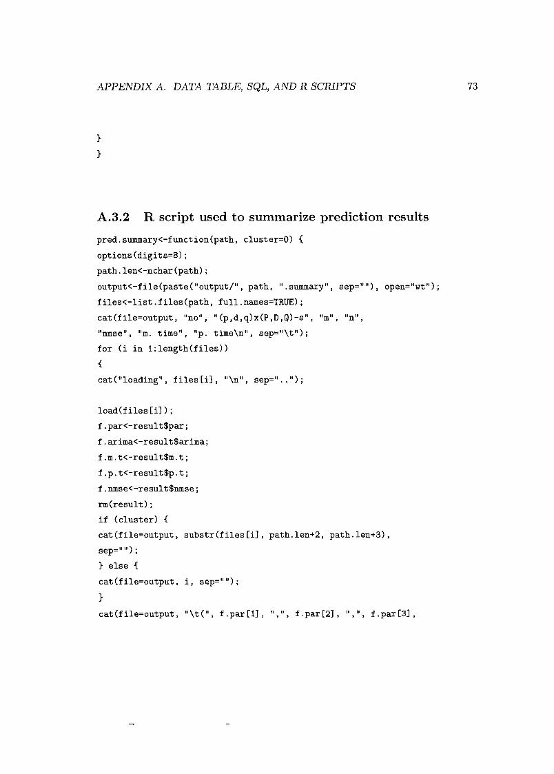
APPENDIX A. DATA TABLE, SQL, AND R SCRIPTS
A.3.2 R script used to summarize prediction results
pred. summary<-f unct ion(path, cluster=O) (:
options (digits=B) ;
path. lent-nchar (path) ;
output<-f ile (paste ("output/", path, " . summary" , sep="" 1, open="wt") ;
files<-list.files(path, full.names=TRUE);
cat(file=output, "no" , "(p,d,q)x(P ,D,Q)-s", "m" , llnlt , "nmse" , I'm. time", "p. time\nM , sep="\tM) ; for (i in l:length(files))
C
cat ("loading", files [i] , "\n" , sep=I1.. "1;
load(f iles [i] ) ;
f.par<-result$par;
f.arima<-result$arima;
f.m.t<-result$m.t;
f.p.t<-result$p.t;
f.nmse<-result$nmse;
rm(resu1t) ;
if (cluster) C cat (f ile=output , substr(f iles [il , path. len+2, path. len+3) , sep=" ") ;
1 else (:
cat (f ile=output , i , sep=" "1 ;
1 cat (f ile=output , "\t (" , f .par C11, " , " , f .par El , " , I' , f .par 131 ,

APPENDIX A. DATA TABLE, SQL, AND R SCRIPTS
cat(I1f inished" , files [il , "in" , sep=". .It);
1 flush (output) ;
close (output) ;
for (i in l:length(f iles)) (
cat ("working on", files Cil , "\n") ; f ile<-paste (dir , "/" , files [i] , sep="") ; cluster<-length(grep("kc3", files [i] ) ) ;
pdq<-substr (f iles [i] , nchar(f iles [ill - 10, nchar (f iles [ill -8) ; season<-substr(f iles[i] , 11, regexpr("-", files [ill [I] -1) ; med<-type [length(grep(I1med" , files [il ))+I] ;
cat ("pdq: " , pdq, "season: " , season, "med: " , med, "\nl1) ;
if (cluster) (
input<-scan(file, what=list('character', 'character', 'integer',
'integer', 'numeric', 'numeric', 'numeric'), skip=l);
1 else C input<-scan(file, what=list('integer', 'character', 'integer',
'integer', 'numeric', 'numeric', 'numeric'), skip=l);
1 for (i in l:length(input~C111)) (
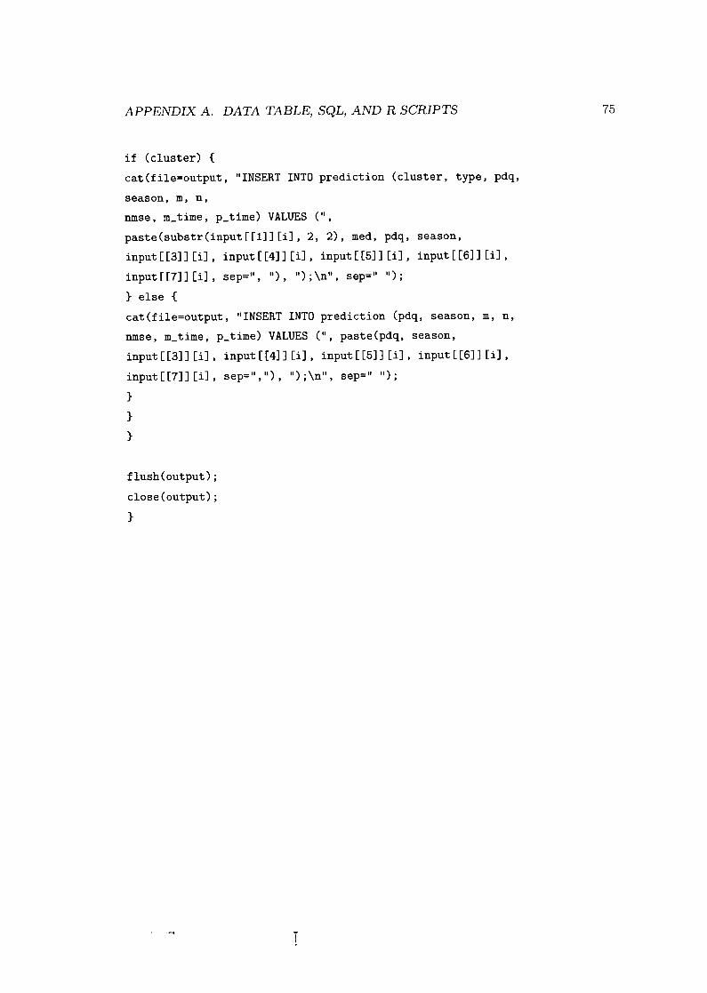
APPENDIX A . DATA TABLE, SQL, AND R SCRIPTS
if (cluster) (
cat(file=output, "INSERT INTO prediction (cluster, type, pdq,
season, m, n,
nmse , m-time , p-t ime) VALUES ( " , paste(substr(inp~t CC11 I Cil , 2, 2), med, pdq, season,
input [ ~311 Cil , input C C4ll Cil , input C C5ll Cil , input C Cell Cil , input C C7l I Cil , sep=lt , ") , ") ; \n" , sep=" ") ;
1 else ( cat(file=output, "INSERT INTO prediction (pdq, season, m, n,
nmse, m-time, p-time) VALUES (I1, paste(pdq, season,
input C C311 [i] , input C C411 Cil , input C [511 Cil , input [ [el I Cil , input [[7]] [i] , sep=", ") , ") ;\nu, sep=" ") ;
> > >
flush (output) ;
close (output) ;
>

Appendix B
AutoClass files
B.l AutoClass model file
The first column of the data file is talk group id. It should be ignored in finding the cluters.
The remaining columns use single-normal-cn model.
#Leo Chen, 2003-Sep-15
#the model file for E-Comm data user clustering
model-index 0 2
ignore 0
single-normal-cn default
;; single-normalxm
;; single~multinomial
B.2 AutoClass influence factor report
#DATA-CLSF-HEADER
#Autoclass CLASSIFICATION for the 617 cases in
#/e-comm/clustering/tg.h/2208/tg2208.db2
#/e-comm/clustering/tg.h/2208/tg2208.hd2

APPENDIX B. AUTOCLASS FILES
#with log-A<X/H> (approximate marginal likelihood) = -6548529.227
#from classification results file
#/e-comm/clustering/tg.h/2208/tg2208.results-bin
#and using models
#/e-comm/clustering/tg.h/2208/tg2208.model - index = 0
#DATA-SEARCH-SUMMARY
#SEARCH SUMMARY 1110 tries over 19 hours 17 minutes 49 seconds
#SUMMARY OF 10 BEST RESULTS
#PROBABILITY exp(-6548529.230) N-CLASSES 24 FOUND ON TRY 653 *SAVED* -1
#PROBABILITY exp(-6592578.320) N-CLASSES 18 FOUND ON TRY 930 *SAVED* -2
#PROBABILITY exp(-6619633.090) N-CLASSES 21 FOUND ON TRY 940
#PROBABILITY exp(-6622783.940) N-CLASSES 24 FOUND ON TRY 323
#PROBABILITY exp(-6626274.570) N-CLASSES 17 FOUND ON TRY 542
#PROBABILITY exp(-6637269.320) N-CLASSES 24 FOUND ON TRY 1084
#PROBABILITY exp(-6657627.910) N-CLASSES 18 FOUND ON TRY 677
#PROBABILITY exp(-6658596.390) N-CLASSES 19 FOUND ON TRY 918
#PROBABILITY exp(-6660040.920) N-CLASSES 18 FOUND ON TRY 528
#PROBABILITY exp(-6671271.570) N-CLASSES 12 FOUND ON TRY 385
DATA-POP-CLASSES
#CLASSIFICATION HAS 24 POPULATED CLASSES
(max global influence value = 10.988)
#Class Log of class Relative
#num strength class strength
00 -8.23e+03 0.00e+00
01 -2.16e+04 0.00e+00
02 -7.69e+03 0.00e+00
03 -7.54e+03 0.00e+00
04 -7.54e+03 0.00e+00
05 -1.48e+04 0.00e+00
06 -6.95e+03 I. 00e+00
Class
weight
144
67
66
31
25
23
22
Normalized
class weight
0.233
0.109
0.107
0.050
0.041
0.037
0.036

APPENDIX B. AUTOCLASS FILES
DATA-CLASS-DIVS
#CLASS DIVERGENCES
#Class (class cross entropy)
#num (w.r.t. global class)
00 1.1 le+04
0 1 5.58e+03
0 2 l.l7e+04
03 l.l9e+04
04 l.l9e+04
05 5.03e+03
06 1.25e+04
07 2.87e+03
08 1.22e+04
0 9 8.31e+03
Class
weight
144
67
66
3 1
25
23
22
2 1
20
20
Normalized
class weight
0.233
0.109
0.107
0.050
0.041
0.037
0.036
0.034
0.032
0.032

APPENDIX B. AUTOCLASS FILES
DATA-NORM-INF-VALS
#ORDERED LIST OF NORMALIZED ATTRIBUTE INFLUENCE
VALUES SUMMED OVER ALL CLASSES
# num description I-*k
4335 Log NCC811 1.000
2490 Log NCC19261 0.999
2986 Log NCC14301 0.998
4039 Log NC C3771 0.998
3732 Log NC C6841 0.998
3832 Log NC C5841 0.996
3184 Log NCC12321 0.996
3831 Log NCC5851 0.995
4043 Log NC C3731 0.992
3927 Log NCC4891 0.992
2487 Log NC C19291 0.992
4209 Log NC C2071 0.991
2506 Log NCC19101 0.991
3804 Log NCC6121 0.990

APPENDIX B. AUTOCLASS FILES
2485 Log NCC19311
3829 Log NCC5871
3948 Log NC 14681
3588 Log NCC8281
3013 Log NC C14031
3158 Log NCC12581
2700 Log NC C17161
3949 Log NC C4671
2699 Log NC 117171
B.3 AutoClass class membership report
# CROSS REFERENCE CLASS => CASE NUMBER MEMBERSHIP
#DATA-CLSF-HEADER
# AutoClass CLASSIFICATION for the 617 cases in
# /e-comm/clustering/tg.h/2208/tg2208.db2
# /e-comm/clustering/tg.h/2208/tg2208.hd2
# with log-A<X/H> (approximate marginal likelihood) = -6548529.227
# from classification results file
# /e-comm/clustering/tg.h/2208/tg2208.results-bin
# and using models
# /e-comm/clustering/tg.h/2208/tg2208.model - index = 0
DATA-CLASS 0
# CLASS = 0
#Case talkgroup NC [Ol NCClI NCC21 NCC3l NC 141 NC 151 NCC6I NC 171
NCC81 NCC91 NCClOl NCClll (Cls Prob)
008 1099.hour.n~ 0 0 0 0 0 0 0 0 0 0 0 0 1.000
009 1100.hour.n~ 0 0 0 0 0 0 0 0 0 0 0 0 1.000
015 1129.hour.n~ 0 0 0 0 0 0 0 0 0 0 0 0 1.000
016 112.hour.n~ 0 0 0 0 0 0 0 0 0 0 0 0 1.000

APPENDIX B. AUTOCLASS FILES
DATA-CLASS I
# CLASS = I
#Case talkgroup NC [Ol NC [I] NCC21 NCC31 NC [41 NC [5] NC [61 NC [7]
NCC81 NCC9I NCC101 NCC111 (Cls Prob)
001 0.hour.m 26 25 24 24 24 25 25 26 26 25 25 23 1.000
003 1089.hour.n~ 6 29 0 0 0 8 0 0 2 80 0 0 1.000
098 1429.hour.n~ 0 0 0 0 0 0 0 0 0 0 0 0 1.000
102 144l.hour.n~ 41 9 13 8 15 44 88 9 26 25 21 25 1.000
109 1474.hour.n~ 31 13 34 35 10 19 30 8 17 7 4 14 1.000
DATA-CLASS 2
# CLASS = 2
#Case talkgroup NC[O] NC[l] NC[2] NC[3] NC[41 NC[5] NC[6] NC[7]
NCC81 NC[91 NCClOl NC[11] (Cls Prob)
033 12118.hour.n~ 0 0 0 0 0 0 0 0 0 0 0 0 1.000
039 12252.hour.n~ 0 0 0 0 0 0 0 0 0 0 0 0 1.000
066 12858.hour.n~ 0 0 0 0 0 0 0 0 0 0 0 0 1.000
069 12872.hour.n~ 0 0 0 0 0 0 0 0 0 0 0 0 1.000
080 13405.hour.n~ 0 0 0 0 0 0 0 0 0 0 0 0 1.000
087 13905.hour.n~ 0 0 0 0 0 0 0 0 0 0 0 0 1.000
094 13931.hour.n~ 0 0 0 0 0 0 0 0 0 0 0 0 1.000
. . . . . .
DATA-CLASS 3
# CLASS = 3
#Case talkgroup N
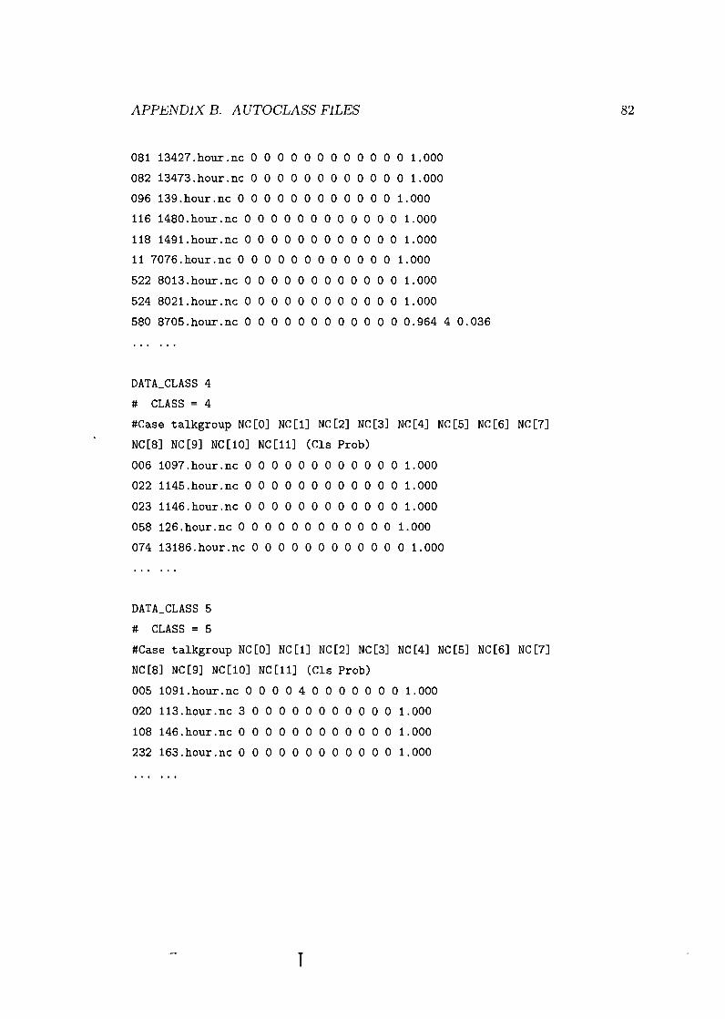
APPENDIX B. AUTOCLASS FILES
DATA-CLASS 4
# CLASS = 4
#Case talkgroup NCCOI N C C l l NCC21 NCC31 NCC41 NCC51 NCC6I NCC71
NCC81 NCC9I N C C l O l NCC111 (Cls Prob)
006 1097 .hour .n~ 0 0 0 0 0 0 0 0 0 0 0 0 1.000
022 1145 .hour .n~ 0 0 0 0 0 0 0 0 0 0 0 0 1.000
023 1146 .hour .n~ 0 0 0 0 0 0 0 0 0 0 0 0 1.000
058 1 2 6 . h o u r . n ~ 0 0 0 0 0 0 0 0 0 0 0 0 1.000
074 13186.hour .n~ 0 0 0 0 0 0 0 0 0 0 0 0 1.000
DATA-CLASS 5
# CLASS = 5
#Case talkgroup NCCOI NCC11 NCC21 NCC3l NCC41 NCC51 NCC6I NCC71
NCC81 NCC91 N C C l O l NCC111 (Cls Prob)
005 1 0 9 l . h o u r . n ~ 0 0 0 0 4 0 0 0 0 0 0 0 1.000
020 1 1 3 . h o u r . n ~ 3 0 0 0 0 0 0 0 0 0 0 0 1.000
108 1 4 6 . h o u r . n ~ 0 0 0 0 0 0 0 0 0 0 0 0 1.000
232 1 6 3 . h o u r . n ~ 0 0 0 0 0 0 0 0 0 0 0 0 1.000

Appendix C
Bayesian network analysis
C. 1 B-Course analysis
Conditional dependency analysis results from B-Course are shown in Figures C.l and C.2.
C.2 Tetrad analysis
Bayesian network analysis results from Tetrad are shown in Figures C.3 and C.4.

APPENDIX C. BAYESIAN NETWORK ANALYSIS
Figure C. 1: B-Coursc a.i~alysis: resull, 1.

APPENDIX C. BAYESIAN NETMTORIC ANALYSIS
Figure C.2: B-Course analysis: result 2.
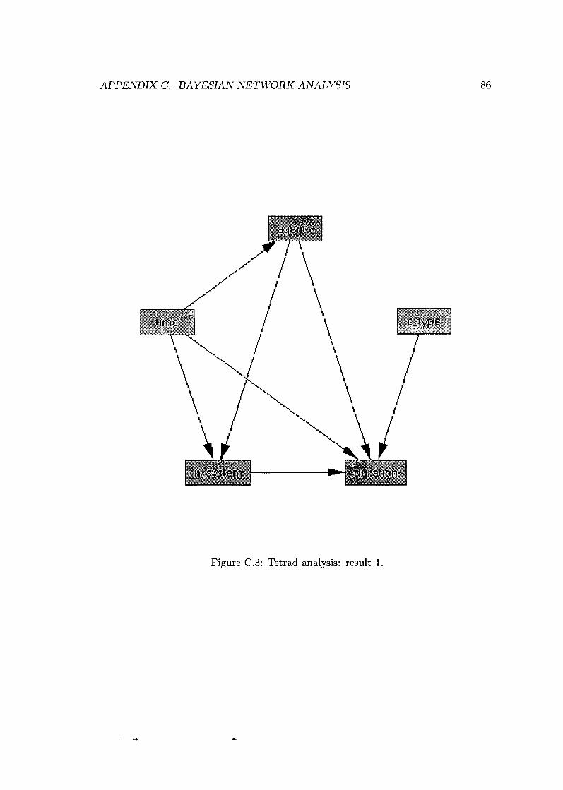
APPENDIX C. BAYESIAN NETWORK ANALYSIS
Figure C.3: Tetrad analysis: result 1.
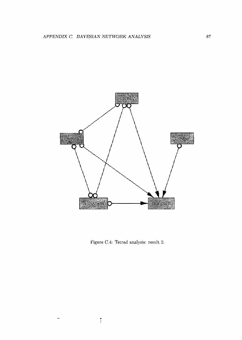
APPENDIX C. BAYESIAN NETWORK ANALYSIS
Figure C.4: Tetrad analysis: result 2.

Bibliography
[I] EComm - Emergency Communications for SW British Columbia. [Online]. Available: http://www.ecomm.bc.ca.
[2] Welcome to Translink. [Online]. Available: http://www.translink.bc.ca.
[3] MIA-COM - supplier of RF and microwave materials, devices, semiconductors, components and wireless systems. [Online]. Available: http://www.macom.com.
[4] EDACS Explained. [Online]. Available: http://www.trunkedradio.net/trunked/ edacs/EDACS-Whitepaper.pdf.
[5] MySQL: The World's Most Popular Open Source Database. [Online]. Available: http://www.mysql.com.
[6] D. Tang and M. Baker, "Analysis of a metropolitan-area wireless network," Wirel. Netw., vol. 8, no. 213, pp. 107-120, March-May 2002.
[71 - , "Analysis of a local-area wireless network," in Proc. of the 6th Annual International Conference on Mobile Computing and Networking. ACM Press, 2000, pp. 1-10.
[8] L. A. Andriantiatsaholiniaina and L. Trajkovi6, "Analysis of user behavior from billing records of a CDPD wireless network," in Proc. of Wireless Local Networks ( W L N ) 2002, Tampa, FL, November 2002, pp. 781-790.
[9] P. Cheeseman and J. Stutz, "Bayesian classification (Autoclass): theory and results," in Advances in Knowledge Discovery and Data Mining, U. M. Fayyad, G. Piatetsky-Shapiro, P. Smyth, and R. Uthurusamy, Eds. AAAI Press/MIT Press, 1996, pp. 61-83.
[lo] L. Kaufman and P. J. Rousseeuw, Finding Groups in Data: A n Introduction to Cluster Analysis. New York, NY: Wiley-Interscience, 1990.

BIBLIOGRAPHY 89
[ll] D. Sharp, N. Cackov, N. Laskovid, Q. Shao. and L. Trajkovid, "Analysis of public safety traffic on trunked land mobile radio systems," JSAC Special Issue on Quality of Service Delivery in Variable Topology Networks, vol. 22, no. 7, pp. 1197-1205, September 2004.
[12] The Autoclass Project. [Online]. Available: http://ic.arc.nasa.gov/ic/projects/ bayes-group/autoclass.
[13] G. McLachlan and D. Peel, Finite Mixture Models. Wiley-Interscience, 2000.
[14] NASA - Computational Sciences Division. [Online]. Available: http: //ic.arc.nasa.gov/ic/projects/bayes-group/index.html.
[15] R. Hansaon, J. Stutz, and P. Cheeseman, "Bayesian classification theory," NASA Arnes Research Center, Artificial Intelligerice Branch, Tech. Rep. FIA-90-12-7-01, 1991.
[16] The Per1 Directory. [Online]. Available: http://www.perl.org.
[17] C. J. Van Rijsbergen, Information Retrieval, 2nd ed. London, Butterworths: Department of Computer Science, University of Glasgow, 1979. [Online]. Available: http://citeseer.ist.psu.edu/vanrijsbergen79information.html
[18] N. Saitou and M. Nei, "The neighbor-joining method: a new method for recon- struction of phylogenetic trees," Mol. Biol. Evol., vol. 8, pp. 406-425, 1987.
[19] M. Ester, H.-P. Kriegel, J. Sander, and X. Xu, "A density-based algorithm for discovering clusters in large spatial databases with noise." in Proc. of the 2nd International Conference on Knowledge Discovery and Data Mining (KDD'96), August 1996, pp. 226-231.
[20] What is an Erlang. [Online]. Available: http://erlang.com/whatis.html.
[21] G. E. Box and G. M. Jenkins, Time Series Analysis: Forecasting and Control. San Francisco, CA: Holden-Day, 1976.
[22] N. K. Groschwitz and G. C. Polyzos, "A time series model of long-term NSFNET backbone traffic," in Proc. of the IEEE International Conference on Communi- cations (ICC'94), vol. 3, May 1994, pp. 1400-1404.
[23] N. H. Chan, Time Series: Applications to Finance. New York, NY: Wiley- Interscience, 2002.
[24] P. J. Brockwell and R. A. Davis, Introduction to Time Series and Forecasting, 2nd ed. New York, NY: Springer-Verlag, 2002.

BIBLIOGRAPHY 90
[25] C. Chat,field, The Analysis of Time Series: An Introduction, 6th ed. Boca Raton, FL: Chapman and Hall/CRC, 2003.
[26] P-Value. [Online]. Available: http://www.isixsigma.com/dictionary/ P-Value-3Ol.htm.
[27] R Development Core Team, R: a language and environment for statistical computing, R Foundation for Statistical Computing, Vienna, Austria, 2004. [Online]. Available: http://www.R- project .org.
[28] R. Ihaka and R. Gentleman, "R: a language for data analysis and graphics," Journal of Computational and Graphical Statistics, vol. 5, no. 3, pp. 299-314, 1996.
[29] B. D. Ripley, "The R project in statistical computing," MSOR Connections. The newsletter of the LTSN Maths, Stats 13 OR Network., vol. 1, no. 1, pp. 23-25, February 2001. [Online]. Available: http://ltsn.mathstore.ac.uk/ newsletter/feb2001/pdf/rproject.pdf
[30] N. Cackov, B. VujiEiC, V. S., and L. TrajkoviC, "Using network activity data to model the utilization of a trunked radio system," in Proc. of the Interna- tional Symposium on Performance Evaluation of Computer and Telecommunica- tion Systems (SPECTS'04), San Jose, CA, July 2004, pp. 517-524.
[31] J. Song and L. Trajkovii.. "Modeling and performance analysis of public safety wireless networks," in Proc. of The First IEEE International Workshop on Radio Resource Management for Wireless Cellular Networks (RRM- WCN), Phoenix, AZ, April 2005, pp. 567-572.
[32] P. Myllymaki, T . Silander, H. Tirri, and P. Uronen, "B-course: A web-based tool for Bayesian and causal data analysis," International Journal on Artificial Intelligence Tools, vol. 11, no. 3, pp. 369-387, December 2002.
[33] B-Course. [Online]. Available: http://b-course.hiit .fi.
[34] Tetrad Project Homepage. [Online]. Available: ht tp://www. phil.cmu.edu/ projectsltetrad.
[351 P. Spirtes, C. Glymour, and R. Scheines, Causation, Prediction, and Search, 2nd ed. Cambridge, MA: MIT Press, 2000.
[36] J . Han and M. Kamber, Data Mining: Concepts and Techniques. San Francisco, CA: Morgan Kaufmann Publishers, 2001.

BIBLIOGRAPHY 91
[37] G. J. McLachlan and T. Krishnan, The EM Algorithm and Extensions. New York; Chichester: Wiley-Interscience, 1997.
[38] R. Scheines, P. Spirtes, C. Glymour, C. Meek, and T. Richard, "The tetrad project: Const,raint based aids to model specification," Multivariate Behavioral Research, vol. 33, no. 1, pp. 65-118, 1998.
[39] Y.-W. Chen, "Traffic behavior analysis and modeling of sub-networks," Interna- tional Journal of Network Management, vol. 12, no. 5, pp. 323-330, September 2002.
[40] P. Cheeseman, J. Kelly, M. Self, J. Stuze, W. Taylor, and D. Freeman, "Autoclass: A Bayesian classification system," in Proc. of the 5th International Conference on Machine Learning, Ann Arbor, MI, June 1988, pp. 54-64.
[41] Making Networks and Applications Perform. [Online]. Available: http: //www.opnet.com.