
Use of structural equation modeling in operations management research: Looking back and forward
22
Use of structural equation modeling in operations management research: Looking back and forward § Rachna Shah * , Susan Meyer Goldstein 1 Operations and Management Science Department, Carlson School of Management, 321, 19th Avenue South, University of Minnesota, Minneapolis, MN 55455, USA Received 10 October 2003; received in revised form 28 March 2005; accepted 3 May 2005 Available online 5 July 2005 Abstract This paper reviews applications of structural equation modeling (SEM) in four major Operations Management journals (Management Science, Journal of Operations Management, Decision Sciences, and Journal of Production and Operations Management Society) and provides guidelines for improving the use of SEM in operations management (OM) research. We review 93 articles from the earliest application of SEM in these journals in 1984 through August 2003. We document and assess these published applications and identify methodological issues gleaned from the SEM literature. The implications of overlooking fundamental assumptions of SEM and ignoring serious methodological issues are presented along with guidelines for improving future applications of SEM in OM research. We find that while SEM is a valuable tool for testing and advancing OM theory, OM researchers need to pay greater attention to these highlighted issues to take full advantage of its potential. # 2005 Elsevier B.V. All rights reserved. Keywords: Empirical research methods; Structural equation modeling; Operations management 1. Introduction Structural equation modeling as a method for measuring relationships among latent variables has been around since early in the 20th century originating in Sewall Wright’s 1916 work (Bollen, 1989). Despite a slow but steady increase in its use, it was not until the monograph by Bagozzi in 1980 that the technique was brought to the attention of a much wider audience of marketing and consumer behavior researchers. While Operations Management (OM) researchers were slow to use this new statistical approach, structural equation modeling (SEM) has more recently become one of the preferred data analysis methods among empirical OM researchers, and articles that employ SEM as the primary data analytic tool now routinely appear in major OM journals. Despite its regular and frequent application in the OM literature, there are few guidelines for the application of SEM and even fewer standards that researchers adhere to in conducting analyses and presenting and interpreting results, resulting in a large www.elsevier.com/locate/dsw Journal of Operations Management 24 (2006) 148–169 § Note: List of reviewed articles is available upon request from the authors. * Corresponding author. Tel.: +1 612 624 4432. E-mail addresses: [email protected] (R. Shah), [email protected] (S.M. Goldstein). 1 Tel.: +1 612 626 0271. 0272-6963/$ – see front matter # 2005 Elsevier B.V. All rights reserved. doi:10.1016/j.jom.2005.05.001
-
Upload
direshan-pillay -
Category
Documents
-
view
214 -
download
1
Transcript of Use of structural equation modeling in operations management research: Looking back and forward
www.elsevier.com/locate/dsw
Journal of Operations Management 24 (2006) 148–169
Use of structural equation modeling in operations
management research: Looking back and forward§
Rachna Shah *, Susan Meyer Goldstein 1
Operations and Management Science Department, Carlson School of Management,
321, 19th Avenue South, University of Minnesota, Minneapolis, MN 55455, USA
Received 10 October 2003; received in revised form 28 March 2005; accepted 3 May 2005
Available online 5 July 2005
Abstract
This paper reviews applications of structural equation modeling (SEM) in four major Operations Management journals
(Management Science, Journal of Operations Management, Decision Sciences, and Journal of Production and Operations
Management Society) and provides guidelines for improving the use of SEM in operations management (OM) research. We
review 93 articles from the earliest application of SEM in these journals in 1984 through August 2003. We document and assess
these published applications and identify methodological issues gleaned from the SEM literature. The implications of
overlooking fundamental assumptions of SEM and ignoring serious methodological issues are presented along with guidelines
for improving future applications of SEM in OM research. We find that while SEM is a valuable tool for testing and advancing
OM theory, OM researchers need to pay greater attention to these highlighted issues to take full advantage of its potential.
# 2005 Elsevier B.V. All rights reserved.
Keywords: Empirical research methods; Structural equation modeling; Operations management
1. Introduction
Structural equation modeling as a method for
measuring relationships among latent variables has
been around since early in the 20th century originating
in Sewall Wright’s 1916 work (Bollen, 1989). Despite
a slow but steady increase in its use, it was not until the
monograph by Bagozzi in 1980 that the technique was
§ Note: List of reviewed articles is available upon request from the
authors.
* Corresponding author. Tel.: +1 612 624 4432.
E-mail addresses: [email protected] (R. Shah),
[email protected] (S.M. Goldstein).1 Tel.: +1 612 626 0271.
0272-6963/$ – see front matter # 2005 Elsevier B.V. All rights reserved
doi:10.1016/j.jom.2005.05.001
brought to the attention of a much wider audience of
marketing and consumer behavior researchers. While
Operations Management (OM) researchers were slow
to use this new statistical approach, structural equation
modeling (SEM) has more recently become one of the
preferred data analysis methods among empirical OM
researchers, and articles that employ SEM as the
primary data analytic tool now routinely appear in
major OM journals.
Despite its regular and frequent application in the
OM literature, there are few guidelines for the
application of SEM and even fewer standards that
researchers adhere to in conducting analyses and
presenting and interpreting results, resulting in a large
.
R. Shah, S.M. Goldstein / Journal of Operations Management 24 (2006) 148–169 149
variance across articles that use SEM. To the best of
our knowledge, there are no reviews of the applica-
tions of SEM in the OM literature, while there are
regular reviews in other research areas that use this
technique. For instance, focused reviews have
appeared periodically in psychology (Hershberger,
2003), marketing (Baumgartner and Homburg, 1996),
MIS (Chin and Todd, 1995; Gefen et al., 2000),
strategic management (Shook et al., 2004), logistics
(Garver and Mentzer, 1999), and organizational
research (Medsker et al., 1994). These reviews have
revealed vast discrepancies and serious flaws in the use
of SEM. Steiger (2001) notes that even SEM textbooks
ignore many important issues, suggesting that
researchers may not have sufficient guidance to use
SEM appropriately.
Due to the complexities involved in using SEM and
problems uncovered in its use in other fields, a review
specific to OM literature seems timely and warranted.
Our objectives in conducting this review are three-
fold. First, we characterize published OM research in
terms of relevant criteria such as software used,
sample size, parameters estimated, purpose for using
SEM (e.g. measurement model development, struc-
tural model evaluation), and fit measures used. In
using SEM, researchers have to make subjective
choices on complex elements that are highly inter-
dependent in order to align research objectives with
analytical requirements. Therefore, our second objec-
tive is to highlight these interdependencies, identify
problem areas, and discuss their implications. Third,
we provide guidelines to improve analysis and
reporting of SEM applications. Our goal is to promote
improved usage of SEM, standardize terminology, and
help prevent some common pitfalls in future OM
research.
2. Overview of structural equation modeling
To provide a basis for subsequent discussion, we
present a brief overview of structural equation
modeling along with two special cases frequently
used in the OM literature. The overview is intended to
be a brief synopsis rather than a comprehensive
detailing of mathematical model specification. There
are a number of books (Maruyama, 1998; Bollen,
1989) and articles dealing with mathematical speci-
fication (Anderson and Gerbing, 1988), key assump-
tions underlying model specification (Bagozzi and Yi,
1988; Fornell, 1983), and other methodological issues
of evaluation and fit (MacCallum, 1986; MacCallum
et al., 1992).
At the outset, we point to a distinction in the use of
two terms that are often used interchangeably in OM:
covariance structure modeling (CSM) and structural
equation modeling (SEM). CSM represents a general
class of models that include ARMA (autoregressive
and moving average) time series models, multi-
plicative models for multi-faceted data, circumplex
models, as well as all SEM models (Long, 1983).
Thus, SEM models are a subset of CSM models. We
restrict the current review to SEM models because
other types of CSM models are rarely used in OM
research.
Structural equation modeling is a technique to
specify, estimate, and evaluate models of linear
relationships among a set of observed variables in
terms of a generally smaller number of unobserved
variables (see Appendix A for detail). SEM models
consist of observed variables (also called manifest or
measured, MV for short) and unobserved variables
(also called underlying or latent, LV for short) that can
be independent (exogenous) or dependent (endogen-
ous) in nature. LVs are hypothetical constructs that
cannot be directly measured, and in SEM are typically
represented by multiple MVs that serve as indicators
of the underlying constructs. The SEM model is an a
priori hypothesis about a pattern of linear relationships
among a set of observed and unobserved variables.
The objective in using SEM is to determine whether
the a priori model is valid, rather than to ‘find’ a
suitable model (Gefen et al., 2000).
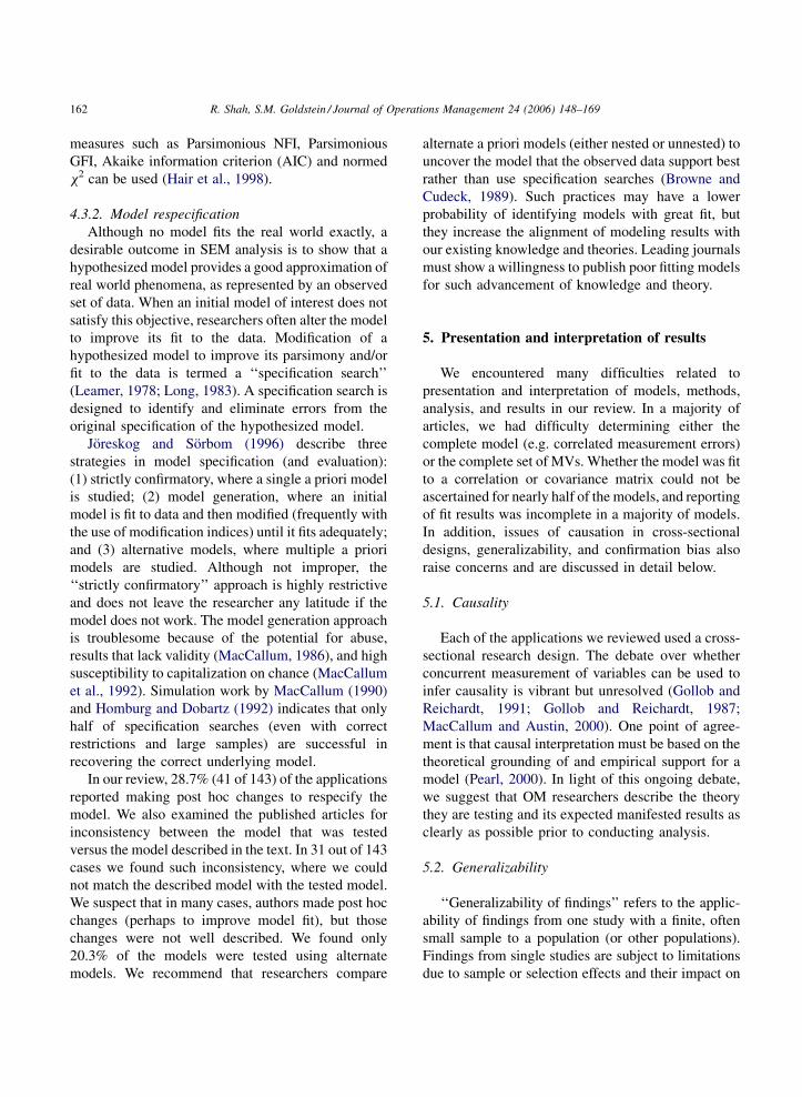
Path analysis and confirmatory factor analysis are
two special cases of SEM that are regularly used in
OM. Path analysis (PA) models specify patterns of
directional and non-directional relationships among
MVs. The only LVs in such models are error terms
(Hair et al., 1998). Thus, PA provides for the testing of
structural relationships amongMVs when theMVs are
of primary interest or whenmultiple indicators for LVs
are not available. Confirmatory factor analysis (CFA)
requires that LVs and their associated MVs be
specified before analyzing the data. This is accom-
plished by restricting the MVs to load on specific LVs
and by designating which LVs are allowed to correlate.
R. Shah, S.M. Goldstein / Journal of Operations Management 24 (2006) 148–169150
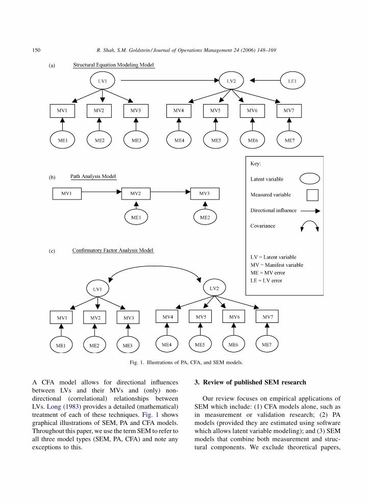
Fig. 1. Illustrations of PA, CFA, and SEM models.
A CFA model allows for directional influences
between LVs and their MVs and (only) non-
directional (correlational) relationships between
LVs. Long (1983) provides a detailed (mathematical)
treatment of each of these techniques. Fig. 1 shows
graphical illustrations of SEM, PA and CFA models.
Throughout this paper, we use the term SEM to refer to
all three model types (SEM, PA, CFA) and note any
exceptions to this.
3. Review of published SEM research
Our review focuses on empirical applications of
SEM which include: (1) CFA models alone, such as
in measurement or validation research; (2) PA
models (provided they are estimated using software
which allows latent variable modeling); and (3) SEM
models that combine both measurement and struc-
tural components. We exclude theoretical papers,
R. Shah, S.M. Goldstein / Journal of Operations Management 24 (2006) 148–169 151
papers using simulation, conventional exploratory
factor analysis (EFA), structural models estimated by
regression models (e.g. models estimated by two
stage least squares), and partial least squares (PLS)
models. EFA models are not included because the
measurement model is not specified a priori (MVs
are not restricted to load on a specific LV and a MV
can load on multiple LVs),1 whereas in SEM, the
model is explicitly defined a priori. The main
objective of regression and PLS models is prediction
of variance explanation in the dependent variable(s)
compared to theory development and testing in the
form of structural relationships (i.e. parameter
estimation) in SEM. This philosophical distinction
between these approaches is critical in deciding
whether to use PLS or SEM (Anderson and Gerbing,
1988). In addition, because assumptions underlying
PLS and regression are less constraining than
SEM, the problems and concerns in conducting
these analyses are significantly different. Therefore,
we do not include regression and PLS models in our
review.
3.1. Journal selection
We considered all OM journals that are recognized
as publishing high quality and relevant empirical OM
research. Recently, Barman et al. (2001) ranked
Management Science (MS), Operations Research
(OR), Journal of Operations Management (JOM),
Decision Sciences (DS), and Journal of Production
and Operations Management Society (POMS) as the
top OM journals in terms of quality. In the past decade,
several additional reviews have examined the quality
and/or relevance of OM journals and have consistently
ranked these journals in the top tier (Vokurka, 1996;
Goh et al., 1997; Soteriou et al., 1998; Malhotra and
Grover, 1998). We do not include OR in our review as
its mission does not include publishing empirical
research.We selected MS, JOM, DS, and POMS as the
journals most representative of high quality and
relevant empirical research in OM. In our review, we
include articles from these four journals that meet our
methodology criteria and do not exclude articles due
to topic of research.
1 Target rotation, rarely used in OM research, is an instance of
EFA in which the model is specified a priori.
3.2. Time horizon and article selection
Rather than use specific search terms for selecting
articles, we manually checked each article of the
reviewed journals. Although more time consuming,
the manual search gave us more control and better
coverage than a ‘‘keyword’’ based search because
there is no widely accepted terminology for research
methods in OM to conduct such a search. In selecting
an appropriate time horizon, we started with the most
recent issue of each journal available until August
2003 and moved backwards in time. Using this
approach, we reviewed all published issues of JOM
from 1982 (Volume 1, Number 1) to 2003 (Volume 21,
Number 4) and POM from 1992 (Volume 1, Number
1) to 2003 (Volume 12, Number 1). For MS and DS,
we moved backward in time until we no longer found
applications of SEM. The earliest application of SEM
in DS was found in 1984 (Volume 15, Number 2) and
the most recent issue reviewed is Volume 34, Number
1 (2003). The incidence of SEM in MS began in 1987
(Volume 34, Number 6) and we reviewed all issues
through Volume 49, Number 8 (2003). The earliest
publication in these two journals corresponds with our
knowledge of the field and seems to have face validity
as such because it coincides with the general
timeframe when SEM was beginning to gain attention
of the wider audience in other literature streams.
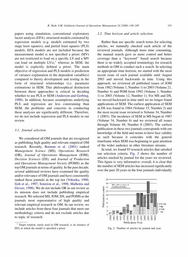
In total, we found 93 research articles that satisfied
our selection criteria. Fig. 2 shows the number of
articles stacked by journal for the years we reviewed.
This figure is very informative: overall, it is clear that
the number of SEM articles has increased significantly
over the past 20 years in the four journals individually
Fig. 2. Number of articles by journal and year.
R. Shah, S.M. Goldstein / Journal of Operations Management 24 (2006) 148–169152
and cumulatively. To assess the growth trend in the use
of SEM, we regress the number of articles on an index
of year of publication (beginning with 1984). We use
both linear and quadratic effects of time in the
regression model.
The regression model is significant (F2,17 = 39.93,
p = 0.000) and indicates that 82% of the variance in
the number of SEM publications is explained by the
linear and quadratic effects of time. Further, the linear
trend is not significant (t = �0.850, p = 0.41), whereas
the quadratic effect is significant (t = 2.94, p = .009).
So the use of SEM has not grown linearly as a function
of time, rather it has accelerated over time. In contrast,
the use of SEM in marketing and psychology grew
steadily over time and there is no indication of its
accelerated use in more recent years (Baumgartner
and Homburg, 1996; Hershberger, 2003).
There are several software programs available for
conducting SEM analysis, and each has idiosyncra-
sies and fundamental requirements for conducting
analysis. In our database, 19.6% of the articles did
not report the software used. Of the articles that
reported the software, LISREL accounted for 48.3%
followed by EQS (18.9%), SAS (9.1%), AMOS
(2.8%), RAMONA (0.7%) and SPSS (0.7%).
LISREL was the first software developed to solve
structural equation models and seems to have
capitalized on its first mover advantage not only in
psychology (MacCallum and Austin, 2000) and
marketing (Baumgartner and Homburg, 1996) but
also in OM.
3.3. Unit of analysis
In our review we found that multiple models were
sometimes presented in one article. Therefore, the unit
of analysis from this point forward (unless specified
otherwise) is the actual applications (one or more
models for each article). A single model is included in
our data set in the following situations: (1) when a
single model is proposed and evaluated using a single
sample; (2) when multiple alternative or nested
models are evaluated using a single sample, only
the final model is included in our analysis; (3) when a
single model is evaluated with either multiple samples
or by splitting a sample, only the model tested with the
verification sample is included in our analysis. Thus,
in these three cases, each article contributed only one
model to the analysis. When more than one model is
evaluated (using single, multiple, or split samples)
each distinct model is included in our analysis. In this
situation, each article contributed more than one
model to the analysis. A total of 143 models were
drawn from the 93 research articles, thus the overall
sample size for the remainder of the paper is 143. Of
the 143 models, we could not determine the method
used for four models. Of the remaining 139 models, 26
are PAs, 38 are CFAs, and 75 are SEMs. There are a
small number of articles that reported models that
never achieved adequate fit (by the authors’ descrip-
tions), and while we include these articles in our
review, the fit measures are omitted from our analysis
to avoid inclusion of data related to models with
inadequate fit.
4. Critical issues in the application of SEM
There are many important issues to consider when
using SEM, whether for evaluating a measurement
model or examining the fit of structural relationships,
separately or simultaneously. Our discussion of issues
is organized into three groups: (1) issues to consider or
address prior to analysis are categorized under the
‘‘pre-analysis’’ stage; (2) issues and concerns to
address during analysis; and (3) issues related to the
post-analysis stage, which includes issues related to
evaluation, interpretation and presentation of results.
Decisions made at each stage are highly interdepen-
dent and significantly impact the quality of results, and
we cross-reference and discuss these interdependen-
cies whenever possible.
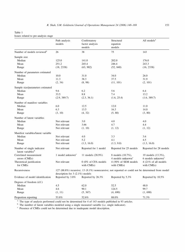
4.1. Issues related to pre-analysis stage
Issues related to the pre-analysis stage need to be
considered prior to conducting SEM analysis and
include conceptual issues, sample size issues, mea-
surement model specification, latent model specifica-
tion, and degrees of freedom issues. A summary of
pre-analysis data from the reviewed OM studies is
presented in Table 1.
4.1.1. Conceptual issues
An underlying assumption of SEM analysis is that
the items or indicators used to measure a LV are
R. Shah, S.M. Goldstein / Journal of Operations Management 24 (2006) 148–169 153
Table 1
Issues related to pre-analysis stage
Path analysis
models
Confirmatory
factor analysis
models
Structural
equation
models
All modelsa
Number of models revieweda 26 38 75 143
Sample size
Median 125.0 141.0 202.0 176.0
Mean 251.2 245.4 246.4 243.3
Range (18, 2338) (63, 902) (52, 840) (16, 2338)
Number of parameters estimated
Median 10.0 31.0 34.0 26.0
Mean 11.3 38.3 37.5 31.9
Range (2, 34) (8, 98) (11, 101) (2, 101)
Sample size/parameters estimated
Median 9.6 6.2 5.6 6.4
Mean 33.5 8.8 7.4 13.2
Range (2.9, 389.7) (2.3, 36.1) (1.6, 25.4) (1.6, 389.7)
Number of manifest variables
Median 6.0 12.5 12.0 11.0
Mean 6.3 13.5 16.3 14.0
Range (3, 10) (4, 32) (5, 80) (3, 80)
Number of latent variables
Median Not relevant 3.0 4.0 4.0
Mean Not relevant 3.66 4.7 4.4
Range Not relevant (1, 10) (1, 12) (1, 12)
Manifest variables/latent variable
Median Not relevant 4.0 3.3 3.6
Mean Not relevant 5.2 4.1 4.5
Range Not relevant (1.3, 16.0) (1.3, 9.0) (1.3, 16.0)
Number of single indicator
latent variablesbNot relevant Reported for 1 model Reported for 25 models Reported for 28 models
Correlated measurement
errors (CMEs)
1 model unknownc 11 models (28.9%) 8 models (10.7%),
4 models unknownc19 models (13.3%),
6 models unknownc
Theoretical justification
for CMEs
Not relevant 0 (0% of CFA models
with CMEs)
4 (50% of SEM models
with CMEs)
4 (21% of all models
with CMEs)
Recursiveness 127 (88.8%) recursive; 13 (9.1%) nonrecursive; not reported or could not be determined from model
description for 3 (2.1%) models
Evidence of model identification Reported by 3.8% Reported by 26.3% Reported by 5.3% Reported by 10.5%
Degrees of freedom (d.f.)
Median 4.5 62.0 52.5 48.0
Mean 4.6 90.1 124.5 99.7
Range (1, 11) (5, 367) (4, 690) (1, 690)
Proportion reporting 53.8% 52.6% 88.0% 71.3%a The type of analysis performed could not be determined for 4 of 143 models published in 93 articles.b The number of latent variables modeled using a single measured variable (i.e. single indicator).c Presence of CMEs could not be determined due to inadequate model description.

R. Shah, S.M. Goldstein / Journal of Operations Management 24 (2006) 148–169154
reflective (i.e. caused by the same underlying LV) in
nature. Yet researchers frequently apply SEM to
formative indicators. Formative (also called causal)
indicators are measures that form or cause the creation
of a LV (MacCallum and Browne, 1993; Bollen,
1989). An example of formative measures is the
amount of beer, wine and hard liquor consumed to
indicate level of mental inebriation (Chin, 1998). It
can be hardly argued that mental inebriation causes the
amount of beer, wine and hard liquor consumption. On
the contrary, the amount of each type of alcoholic
beverage affects the level of mental inebriation.
Formative indicators do not need to be highly
correlated or have high internal consistency (Bollen,
1989). In this example, an increase in beer consump-
tion does not imply an increase in wine or hard liquor
consumption. Measurement of formative indicators
requires an index (as opposed to developing a scale
when using reflective indicators), and can be modeled
using SEM, but requires additional constraints
(Bollen, 1989; MacCallum and Browne, 1993). Using
SEM without additional constraints makes the
resulting estimates invalid (Fornell et al., 1991) and
the model statistically unidentified (Bollen and
Lennox, 1991).
Another underlying assumption for SEM is that the
theoretical relationships hypothesized in the models
being tested represent actual relationships in the
studied population. SEM assesses how closely the
observed data correspond to the expected patterns
and requires that relationships represented by the
model are well established and amenable to accurate
measurement in the population. SEM is not recom-
mended for exploratory research when the measure-
ment structure is not well defined or when the theory
that underlies patterns of relationships among LVs is
not well established (Brannick, 1995; Hurley et al.,
1997).
Thus, researchers need to carefully consider: (1)
type of items, (2) state of underlying theory, and (3)
stage of development of measurement instrument,
prior to using SEM. For formative measurement items,
researchers should consider alternative techniques
such as SEM using formative indicators (MacCallum
and Browne, 1993) and components-based approaches
such as partial least squares (Cohen et al., 1990).
When the underlying theory or the measurement
structure is not well developed, simpler data analytic
techniques such as EFA and regression analysis may
be more appropriate (Hurley et al., 1997).
4.1.2. Sample size issues
Adequacy of sample size has a significant impact
on the reliability of parameter estimates, model fit,
and statistical power. Using a simulation experiment
to examine the effect of varying sample size to
parameter estimate ratios, Jackson (2003) reports that
smaller sample sizes are generally characterized by
parameter estimates with low reliability, greater
bias in x2 and RMSEA fit statistics, and greater
uncertainty in future replication. How large a sample
should be for SEM is deceptively difficult to
determine because it is dependent upon several
characteristics such as number of MVs per LV
(MacCallum et al., 1996), degree of multivariate
normality (West et al., 1995), and estimation method
(Tanaka, 1987). Suggested approaches for determin-
ing sample size include establishing a minimum (e.g.,
200), having a certain number of observations per
MV, having a certain number of observations per
parameters estimated (Bentler and Chou, 1987;
Bollen, 1989; Marsh et al., 1988), and through
conducting power analysis (MacCallum et al., 1996).
While the first two approaches are simply rules
of thumbs, the latter two have been studied
extensively.
Table 1 reports the results of analysis of SEM
applications in the OM literature related to sample size
and number of parameters estimated. The smallest
sample sizes for PA (n = 18), CFA (n = 63), and SEM
(n = 52) are significantly smaller than established
guidelines for models with even minimal complexity
(MacCallum et al., 1996; Marsh et al., 1988).
Additionally, 67.9% of all models have ratios of
sample size to parameters estimates of less than 10:1
and 35.7% of models have ratios of less than 5:1. The
lower end of both sample size and sample size to
parameter estimate ratios are significantly smaller in
the reviewed OM research than those studied by
Jackson (2003), indicating that the OM literature may
be highly susceptible to the negative outcomes
reported in his study.
Statistical power (i.e. the ability to detect and
reject a poor model) is critical to SEM analysis
because, in contrast to traditional hypothesis testing,
the goal in SEM analysis is to produce a non-
R. Shah, S.M. Goldstein / Journal of Operations Management 24 (2006) 148–169 155
significant result between sample data and the
implied covariance matrix derived from model
parameter estimates. Yet, a non-significant result
may also be due to a lack of ability (i.e. power) to
detect model misspecification. Few studies in our
review mentioned power and none estimated power
explicitly. Therefore, we employed MacCallum et al.
(1996), who define minimum sample size as a
function of degrees of freedom that is needed for
adequate power (0.80) to detect close model fit, to
assess the power of models in our sample. (We were
not able to assess power for 41 of 143 models due to
insufficient information.) Our analysis indicates that
37% of the models have adequate power and 63% do
not. These proportions are consistent with similar
analyses in psychology (MacCallum and Austin,
2000), MIS (Chin and Todd, 1995), and strategy
(Shook et al., 2004), and have not changed since
1960 (Sedlmeier and Gigenrenzer, 1989). We
recommend that future researchers use MacCallum
et al. (1996) to calculate the minimum sample size
needed to ensure adequate statistical power.
4.1.3. Degrees of freedom and model
identification
Degrees of freedom are calculated as follows:
d:f: ¼ ð1=2Þf pð pþ 1Þg � q, where p is the number
of MVs, ð1=2Þf pð pþ 1Þg is the number of equations
(or alternately, the number of distinct elements in the
input matrix ‘‘S’’), and q is the effective number of
free (unknown) parameters to be estimated minus the
number of implied variances. As the formula
indicates, degrees of freedom is a function of model
specification in terms of the number of equations and
the effective number of free parameters that need to be
estimated.
When the effective number of free parameters is
exactly equal to the number of equations (that is, the
degrees of freedom are zero), the model is said to be
‘‘just-identified’’ or ‘‘saturated’’. Just-identified mod-
els provide an exact solution for parameters (i.e. point
estimates with no confidence intervals). When the
effective number of free parameters is greater than the
number of equations (degrees of freedom are less than
zero), the model is ‘‘under-identified’’ and sufficient
information is not available to uniquely estimate the
parameters. Under-identified models may not con-
verge during model estimation, and when they do, the
parameter estimates they provide are not reliable and
overall fit statistics cannot be interpreted (Rigdon,
1995). For models in which there are fewer unknowns
than equations (degrees of freedom are one or greater),
the model is ‘‘over-identified’’. An over-identified
model is highly desirable because more than one
equation is used to estimate at least some of the
parameters, significantly enhancing reliability of the
estimate (Bollen, 1989).
Model identification is a complex issue and while
non-negative degrees of freedom is a necessary
condition, additional conditions such as establishing
a scale for each LV are frequently required (for a
detailed discourse on sufficiency conditions, see Long,
1983; Bollen, 1989). In our review, degrees of freedom
were not reported for 41 (28.7%) models (see Table 1).
We recalculated the degrees of freedom independently
for each reviewed model to assess discrepancies
between the reported and our calculated degrees of
freedom. Wewere not able to reproduce the degrees of
freedom for 18 applications based on authors’
descriptions of their models. This lack of reproduci-
bility may be due in part to poor model description or
to correlated errors in the measurement or latent
variable models that are not stated in the text. We also
examined whether the issue of identification was
explicitly addressed for each model. One author
reported that the estimated model was not identified
and only 10.5% mentioned anything about model
identification. Perhaps the issue of identification was
considered implicitly because many software pro-
grams provide a warning message if a model is not
identified.
Model identification has a significant impact on
parameter estimates: in an unidentified model, more
than one set of parameter estimates could generate the
observed data and a researcher has no way to choose
among the various solutions because each is equally
valid (or invalid, if you wish). Degrees of freedom are
critically linked to the minimum sample size required
for adequate model fit; the greater the degrees of
freedom, the smaller the sample size needed for a
given level of model fit (MacCallum et al., 1996).
Calculating and reporting the degrees of freedom are
fundamental to understanding the specified model, its
identification, and its fit. Thus, we recommend that
degrees of freedom and model identification should be
reported for every tested model.
R. Shah, S.M. Goldstein / Journal of Operations Management 24 (2006) 148–169156
4.1.4. Measurement model specification
4.1.4.1. Number of items (MVs) per LV. It is generally
accepted that multiple MVs should measure each LV
but the number of MVs that should be used is less
clear. A ratio of fewer than three MVs per LV is of
concern because the model is statistically unidentified
in the absence of additional constraints (Long, 1983).
A large number of MVs per LV is advantageous as it
helps to compensate for a small sample (Marsh et al.,
1988) but disadvantageous as it means more para-
meters to estimate, requiring a larger sample size for
adequate power. A large number of MVs per LV also
makes it difficult to parsimoniously represent the
measurement structure constituting the set of MVs
(Anderson and Gerbing, 1984). In cases where a large
number of MVs are needed to represent a LV, Bagozzi
and Heatherton (1994) suggest four methods to reduce
the number of MVs per LV. In our review, 24% of CFA
models (9 of 38) and 39% of SEM models (29 of 75)
had a MV:LV ratio of less than 3. Generally, these
applications did not explicitly discuss identification
issues or additional constraints. The number of MVs
per LV characteristic is not applicable to PA models.
4.1.4.2. Single indicator constructs. We identified
LVs represented by a single indicator in 2.6% of CFA
models and 33.3% of SEM models in our sample (not
applicable to PA models). The low occurrence of
single indicator variables for CFA is not surprising
because the central objective of CFA is construct
measurement. However, the relatively high occurrence
of single indicator constructs in SEM models is
troublesome because single indicators ignore mea-
surement reliability, one of the challenges SEM is
designed to circumvent (Bentler and Chou, 1987). The
single indicator issue is also tied to model identifica-
tion as discussed above. Single indicators are only
sufficient when one measure perfectly represents a
concept, a rare situation, or when measurement
reliability is not an issue. Generally, single MVs
should be modeled as MVs rather than LVs.
4.1.4.3. Correlated measurement errors. Measure-
ment errors should sometimes be modeled as
correlated, for instance, in a longitudinal study when
the same item is measured at two points in time
(Bollen, 1989 p. 232). The statistical effect of
correlated error terms is the same as double loading,
but the substantive meaning is significantly different.
Double loading implies that each MV is affected by
two underlying LVs. Fundamental to LV unidimen-
sionality is that eachMV load on one LVwith loadings
on all other LVs restricted to zero. Because adding
correlated measurement errors to SEM models nearly
always improves model fit, they are often used post
hoc without improving the substantive interpretation
of the model (Fornell, 1983; Gerbing and Anderson,
1984) and making reliability estimates ambiguous
(Bollen, 1989 p. 222).
To the best of our knowledge, our sample contains
no instances of double loading MVs but we found a
number of models with correlated measurement
errors: 3.8% of PA, 28.9% of CFA, and 10.7% of
SEMmodels. We read the text of each article carefully
to determine whether the authors provided any
theoretical justification for using correlated errors or
whether they were introduced simply to improve
model fit. In more than half of the applications, no
justification was provided. Correlated measurement
errors should be used only when warranted on
theoretical or methodological grounds (Fornell,
1983) and their statistical and substantive impact
should be explicitly discussed.
4.1.5. Latent model specification
4.1.5.1. Recursive/non-recursive models. Models are
non-recursive when they contain reciprocal causation,
feedback loops, or correlated error terms (Bollen,
1989, p. 83). In such models, the matrix representing
latent exogenous variables (B; seeAppendixA formore
detail) has non-zero elements both above and below the
diagonal. If B is lower triangular and the errors in
equations are uncorrelated, then the model is called
recursive (Hair et al., 1998). Non-recursive models
require additional restrictions for the model to be
identified, for the stability of estimated reciprocal
effects, and for the interpretation of measures of
variation accounted for in the endogenous variables (for
a more detailed treatment of non-recursive models, see
Long, 1983; Teel et al., 1986). In our review, we
examined each application for recursive and non-
recursive models due to either simultaneous effects or
correlated errors in equations.Whilewe did not observe
any instances of simultaneous effects, we found that in
9.1% of the models, either the authors defined their
model as non-recursiveor a careful readingof the article
R. Shah, S.M. Goldstein / Journal of Operations Management 24 (2006) 148–169 157
led to such a conclusion. However, even when authors
explicitly stated that they were testing a non-recursive
model, we saw little if any explanation of issues such as
model identification in the text. We recommend that if
non-recursive models are specified, additional restric-
tions and implications for model identification are
explicitly stated in the paper.
4.2. Issues related to data analysis
Data analysis issues comprise examining sample
data for distributional characteristics and generating
an input matrix. Distributional characteristics of the
data impact researchers’ choices of estimation
method, and the type of input matrix impacts the
selection of software used for analysis.
4.2.1. Data screening
Data screening is critical to prepare data for SEM
analysis (Hair et al., 1998). Screening through
exploratory data analysis includes investigating for
missing data, influential outliers, and distributional
characteristics. Significant missing data result in
convergence failures, biased parameter estimates,
and inflated fit indices (Brown, 1994; Muthen et al.,
1987). Influential outliers are linked to normality and
skewness issues with MVs. Assessing data normality
(along with skewness and kurtosis) is important
because many model estimation methods are based on
an assumption of normality. Non-normal data may
result in inflated goodness of fit statistics and
underestimated standard errors (MacCallum et al.,
1992), although these effects are lessened with larger
sample sizes (Lei and Lomax, 2005).
In our review, only a handful of applications
discussed missing data. In the psychology literature,
listwise deletion, pairwise deletion, data imputation
and full information maximum likelihood (FIML)
methods are commonly used to manage missing data
(Marsh, 1998). Results from Monte Carlo simulation
examining the performance of these four methods
indicate the superiority of FIML, leading to the lowest
rate of convergence failures, least bias in parameter
estimates, and lowest inflation in goodness of fit
statistics (Enders and Bandalos, 2001; Brown, 1994).
FIML method is currently available in LISREL
(version 8.50 and above), SYSTAT (RAMONA) and
AMOS.
We found that for 26.6% of applications, normality
was discussed qualitatively in the text of the reviewed
articles. Estimation methods such as maximum
likelihood ratio and generalized least square assume
normality, although some non-normality can be
accommodated (Hu and Bentler, 1998; Lei and
Lomax, 2005). Weighted least square, ordinary least
square, and asymptotically distribution free estimation
methods do not require normality. Additionally, ‘‘ML,
Robust’’ in EQS software adjusts model fit and
parameter estimates for non-normality. Finally,
researchers can transform non-normal data, although
serious problems have been noted with data transfor-
mation (cf. Satorra, 2001). We suggest that some
discussion of data screening methods be included
generally, and normality be discussed specifically in
relation to the choice of estimation method.
4.2.2. Type of input matrix
While raw data can be used as input for SEM
analysis, a covariance (S) or correlation (R) matrix is
generally used. In our review of the OM literature, no
papers report using raw data, 30.8% report using S,
and 25.2% report using R (44.1% of applications did
not report the type of matrix used to conduct analysis).
Seven of 44 applications using S and 25 of 36
applications using R provide the input matrix in the
paper. Not providing the input matrix makes it
impossible to replicate the results reported by the
author(s).
While conventional estimation methods in SEM are
based on statistical distribution theory that is
appropriate for S but not for R, there are interpreta-
tional advantages to using R: if MVs are standardized
and the model is fit to R, then parameter estimates can
be interpreted in terms of standardized variables.
However, it is not correct to fit a model to R while
treating R as if it were a covariance matrix. Cudeck
(1989) conducted exhaustive analysis on the implica-
tions of treating R as if it were S and concludes that the
consequences depend on the properties of the model
being fitted: standard errors, confidence intervals and
test statistics for the parameter estimates are incorrect
in all cases. In some cases, parameter estimates and
values of fit indices are also incorrect.
Software programs commonly used to conduct
SEM deal with this issue in different ways. Correct
estimation of a correlation matrix can be done in
R. Shah, S.M. Goldstein / Journal of Operations Management 24 (2006) 148–169158
LISREL (Joreskog and Sorbom, 1996) but requires the
user to introduce specific parameter constraints.
Although not widely used in OM, RAMONA (Browne
and Mels, 1998), EQS (Bentler, 1989) and SEPATH
(Steiger, 1999) automatically provide correct estima-
tion with a correlation matrix. Currently, AMOS
cannot analyze correlation matrices. In our review, we
found 24 instances where authors reported using a
correlation matrix with LISREL (out of 69 models run
with LISREL) but most did not mention the necessary
additional constraints. We found one instance of using
AMOS with a correlation matrix.
Given the lack of awareness among users about the
treatment of R versus S by various software programs,
we direct readers’ attention to a test devised by
MacCallum and Austin (2000) to help users determine
whether a particular SEM program provides correct
estimation of a model fit to a correlation matrix.
Otherwise, it is preferable to fit models to covariance
matrices, thus insuring correct results.
4.2.3. Estimation methods
A variety of estimation methods such as maximum
likelihood ratio (ML), generalized least square (GLS),
weighted and unweighted least square (WLS andULS),
asymptotically distribution free (ADF), and ordinary
least square (OLS) are available. Their use depends
upon the distributional properties of theMVs, and each
has computational advantages and disadvantages
relative to the others. For instance, ML assumes data
are univariate andmultivariate normal and requires that
the input data matrix be positive definite, but it is
Table 2a
Issues related to data analysis for structural model
Number of models reporting (n = 143)
x2 107
x2, p-value 76
GFI 84
AGFI 59
RMR (or RMSR) 51
RMSEA 51
NFI 49
NNFI (or TLI) 62
CFI 73
IFI (or BL89) 16
Normed x2 (x2/d.f.) reported 52
Normed x2 calculated 98b
a One model reported RMR = 145.4; this data point omitted as an outb Data not available to calculate others.
relatively unbiased under moderate violations of
normality (Bollen, 1989). GLS assumes normality
but does not impose the restriction of a positive definite
input matrix. ADF has few distributional assumptions
but requires very large sample sizes for accurate
estimates. OLS, the simplest method, has no distribu-
tional assumptions and is computationally the most
robust, but it is scale invariant and does not provide fit
indices or standard errors for estimates.
Forty-eight percent of applications in our review
did not report the estimation method used. Of the
applications that reported the estimation method, a
majority (68.9%) used ML. Estimation method, data
normality, sample size, and model specification are
inextricably linked and must be considered simulta-
neously by the researcher. We suggest that authors
explicitly state the estimation method used and link it
to the properties of the observed variables.
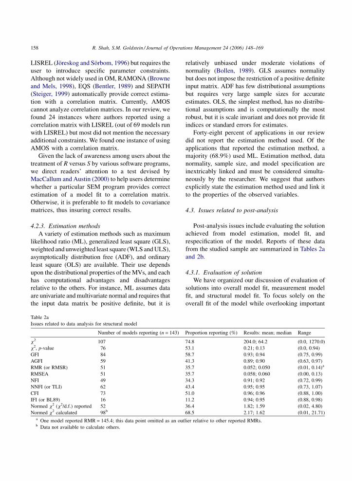
4.3. Issues related to post-analysis
Post-analysis issues include evaluating the solution
achieved from model estimation, model fit, and
respecification of the model. Reports of these data
from the studied sample are summarized in Tables 2a
and 2b.
4.3.1. Evaluation of solution
We have organized our discussion of evaluation of
solutions into overall model fit, measurement model
fit, and structural model fit. To focus solely on the
overall fit of the model while overlooking important
Proportion reporting (%) Results: mean; median Range
74.8 204.0; 64.2 (0.0, 1270.0)
53.1 0.21; 0.13 (0.0, 0.94)
58.7 0.93; 0.94 (0.75, 0.99)
41.3 0.89; 0.90 (0.63, 0.97)
35.7 0.052; 0.050 (0.01, 0.14)a
35.7 0.058; 0.060 (0.00, 0.13)
34.3 0.91; 0.92 (0.72, 0.99)
43.4 0.95; 0.95 (0.73, 1.07)
51.0 0.96; 0.96 (0.88, 1.00)
11.2 0.94; 0.95 (0.88, 0.98)
36.4 1.82; 1.59 (0.02, 4.80)
68.5 2.17; 1.62 (0.01, 21.71)
lier relative to other reported RMRs.

R. Shah, S.M. Goldstein / Journal of Operations Management 24 (2006) 148–169 159
Table 2b
Issues related to data analysis for measurement model
Number of
models reporting
(n = 143)
Proportion
reporting
(%)
Reliability assessment 123 86.0
Unidimensionality assessment 94 65.7
Discriminant validity addressed 99 69.2
Validity issues addressed
(R2; variance explained)
76 53.1
Path coefficients
(confidence intervals)
138 (3) 96.5 (2.1)
Path t-statistics (standard errors) 90 (21) 62.9 (14.7)
Residual information/analysis
provided
19 13.3
Specification search conducted
for model respecification
20 14.0
Modification indices used
for model respecification
21 14.7
Alternative models compared 29 20.3
Inconsistency between described
and tested models
31 21.7
Cross-validation sample used 22 15.4
Split sample approach used 27 18.9
information about parameters is a common error that
we encountered in our review. A model with good
overall fit but yielding nonsensical parameter esti-
mates is not a useful model.
4.3.1.1. Overall model fit. Assessing a model’s fit is
one of the more complicated aspects of SEM because,
unlike traditional statistical methods, it relies on non-
significance. Historically, the most popular index used
to assess the overall goodness of fit has been the x2-
statistic, although its conclusions regarding model
significance are generally ignored. The x2-statistic is
inherently biased when the sample size is large but is
dependent on distributional assumptions associated
with large samples. Additionally, a x2-test offers a
dichotomous decision strategy (accept /reject) for
assessing the adequacy of fit implied by a statistical
decision rule (Bollen, 1989). In light of these issues,
numerous alternative fit indices have been developed
to quantify the degree of fit along a continuum (see
Joreskog, 1993; Tanaka, 1993; Bollen, 1989, pp. 256–
289; Mulaik et al., 1989 for comprehensive reviews).
Fit indices are commonly distinguished as either
absolute or incremental (Bollen, 1989). In general,
absolute fit indices indicate the degree to which the
hypothesized model reproduces the sample data, and
incremental fit indices measure the proportional
improvement in fit when the hypothesized model is
compared with a restricted, nested baseline model (Hu
and Bentler, 1998).
Absolute measures of fit: The most basicmeasure of
absolute fit is the x2-statistic. Other commonly used
measures include root mean square error of approx-
imation (RMSEA), root mean square residual (RMR or
SRMR), goodness-of-fit index (GFI) and adjusted
goodness of fit (AGFI). GFI and AGFI increase as
goodness of fit increases and are bounded above by
1.00, while RMSEA and RMR decrease as goodness of
fit increases and are bounded below by zero (Browne
and Cudeck, 1989). Ninety-four percent of the
applications we reviewed report at least one of these
measures (Table 2a). Although the frequency of use and
the magnitude of each of these measures are similar to
those reported in marketing by Baumgartner and
Homburg (1996), the ranges in our sample are much
wider indicating greater variability in empirical OM
research. The variability may be an indication of more
complex models and/or a less established theory base.
Incremental fit measures: Incremental fit measures
compare the model under study to two reference
models: (1) a worst case or null model, and (2) an ideal
model that perfectly represents the modeled phenom-
ena in the studied population. While there are many
incremental fit indices, some of the most popular are
normed fit index (NFI), non-normed fit index (NNFI or
TLI), comparative fit index (CFI) and incremental fit
index (IFI or BL89). Sixty-nine percent of the
reviewed studies report at least one of the four
measures (Table 2a). An additional fit index that is
frequently used is the normed x2 which is reported for
36.4% of models. Because the x2-statistic by itself is
beset with problems, the ratio of x2 to degrees of
freedom (x2/d.f.) is informative because it corrects for
model size. Additionally, we calculated the normed x2
for all models that reported x2 and either reported
degrees of freedom or enough model specification
information to allow us to ascertain the degrees of
freedom (68.5% of all applications) and found a
median of 1.62 (range 0.01, 21.71). Small values of
normed x2 (<1.0) can indicate an over-fitted model
and higher values (>3.0–5.0) can indicate an under-
parameterized model (Joreskog, 1969).
A brief summary of the effects on fit indices of
small samples, normality violations, model misspe-
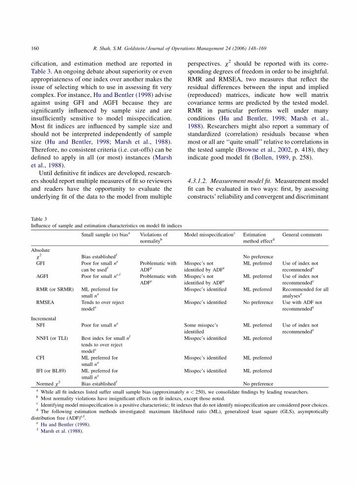
R. Shah, S.M. Goldstein / Journal of Operations Management 24 (2006) 148–169160
cification, and estimation method are reported in
Table 3. An ongoing debate about superiority or even
appropriateness of one index over another makes the
issue of selecting which to use in assessing fit very
complex. For instance, Hu and Bentler (1998) advise
against using GFI and AGFI because they are
significantly influenced by sample size and are
insufficiently sensitive to model misspecification.
Most fit indices are influenced by sample size and
should not be interpreted independently of sample
size (Hu and Bentler, 1998; Marsh et al., 1988).
Therefore, no consistent criteria (i.e. cut-offs) can be
defined to apply in all (or most) instances (Marsh
et al., 1988).
Until definitive fit indices are developed, research-
ers should report multiple measures of fit so reviewers
and readers have the opportunity to evaluate the
underlying fit of the data to the model from multiple
Table 3
Influence of sample and estimation characteristics on model fit indices
Small sample (n) biasa Violations of
normalitybM
Absolute
x2 Bias establishedf
GFI Poor for small ne
can be usedfProblematic with
ADFeM
id
AGFI Poor for small ne,f Problematic with
ADFeM
id
RMR (or SRMR) ML preferred for
small neM
RMSEA Tends to over reject
modeleM
Incremental
NFI Poor for small ne S
id
NNFI (or TLI) Best index for small nf
tends to over reject
modele
M
CFI ML preferred for
small neM
IFI (or BL89) ML preferred for
small neM
Normed x2 Bias establishedf
a While all fit indexes listed suffer small sample bias (approximatelyb Most normality violations have insignificant effects on fit indexes, ec Identifying model misspecification is a positive characteristic; fit indexd The following estimation methods investigated: maximum likelih
distribution free (ADF)e,f.e Hu and Bentler (1998).f Marsh et al. (1988).
perspectives. x2 should be reported with its corre-
sponding degrees of freedom in order to be insightful.
RMR and RMSEA, two measures that reflect the
residual differences between the input and implied
(reproduced) matrices, indicate how well matrix
covariance terms are predicted by the tested model.
RMR in particular performs well under many
conditions (Hu and Bentler, 1998; Marsh et al.,
1988). Researchers might also report a summary of
standardized (correlation) residuals because when
most or all are ‘‘quite small’’ relative to correlations in
the tested sample (Browne et al., 2002, p. 418), they
indicate good model fit (Bollen, 1989, p. 258).
4.3.1.2. Measurement model fit. Measurement model
fit can be evaluated in two ways: first, by assessing
constructs’ reliability and convergent and discriminant
odel misspecificationc Estimation
method effectdGeneral comments
No preference
isspec’s not
entified by ADFeML preferred Use of index not
recommendede
isspec’s not
entified by ADFeML preferred Use of index not
recommendede
isspec’s identified ML preferred Recommended for all
analysese
isspec’s identified No preference Use with ADF not
recommendede
ome misspec’s
entified
ML preferred Use of index not
recommendede
isspec’s identified ML preferred
isspec’s identified ML preferred
isspec’s identified ML preferred
No preference
n < 250), we consolidate findings by leading researchers.
xcept those noted.
es that do not identify misspecification are considered poor choices.
ood ratio (ML), generalized least square (GLS), asymptotically
R. Shah, S.M. Goldstein / Journal of Operations Management 24 (2006) 148–169 161
validity, and second, by examining the individual path
(parameter) estimates (Bollen, 1989).
Various indices of reliability can be computed to
summarize how well LVs are measured by their MVs
individually or jointly (individual item reliability,
composite reliability, and average variance extracted;
cf. Bagozzi and Yi, 1988; Fornell and Larcker, 1981).
Our initial attempt to report reliability measures used
by the authors proved difficult due to the diversity of
methods used. Therefore, we limit our review to
whether authors report at least one of the various
measures. Overall, 86.0% of the applications describe
some form of reliability assessment. We recommend
that authors report at least one measure of construct
reliability based on estimated model parameters (e.g.
composite reliability or average variance extracted)
(Bollen, 1989).
Cronbach alpha is an inferior measure of reliability
because in most cases it is only a lower bound on
reliability (Bollen, 1989). In our review we found that
Cronbach alpha was frequently presented as proof to
establish unidimensionality. It is not sufficient for this
purpose because a scale may not be unidimensional
even if it has high reliability (Gerbing and Anderson,
1984). Our review also examined how published
research dealt with the issue of discriminant validity.
We found that 69.2% of all applications included
evidence of discriminant validity. Our review indicates
that despite a lack of standardization in the reported
measures, most published research in OM includes
some measure of reliability, unidimensionality and
validity.
Another way to assess measurement model fit is to
evaluate path estimates. In evaluating path estimates,
sign (positive or negative), strength, and significance
should be aligned with theory. The magnitude of
standard errors associated with path estimates should
be small; a large standard error indicates an unstable
parameter estimate that is subject to sampling error.
Although recommended but rarely used in practice,
the 90% confidence interval (CI) around each path
estimate is very useful (Browne and Cudeck, 1993).
The CI provides an explicit indication of the degree of
parameter estimate precision. Additionally, the sta-
tistical significance of path estimates can be inferred
from the 90% CI: if the 90% CI includes zero, then the
path estimate is not significantly different from zero
(at a = 0.05). Overall, confidence intervals are very
informative and we recommend their use in future
studies. In our review, we found that 96.5% of the
applications report path coefficients, 62.9% provide t
statistics, 14.7% provide standard errors, and 2.1%
report confidence intervals.
4.3.1.3. Structural model fit. In SEM models, the
latent variable model represents the structural model
fit, and generally, the hypotheses of interest. In PA
models that do not have LVs, the hypotheses of interest
are generally represented by the paths between MVs.
Like measurement model fit, the sign, magnitude and
statistical significance of the structural path coeffi-
cients are examined in testing the hypotheses.
Researchers should recognize the important distinc-
tion between variance fit (explained variance in
endogenous variables as measured by R2 for each
structural equation) and covariance fit (overall good-
ness of fit, such as that tested by a x2-test). Authors
emphasize covariance fit a great deal more than
variance fit; in our review, 53.1% of the models
presented evidence of the variance fit compared to 96%
that presented at least one index of overall fit. It is
important to distinguish between these two types of fit
because a model might fit well but not explain a
significant amount of variation in endogenous variables
or conversely, fit poorly and explain a large amount of
variation in endogenous variables (Fornell, 1983).
In summary, we suggest that fit indices should
not be regarded as measures of usefulness of a model.
They each contain some information aboutmodel fit but
none about model plausibility (Browne and Cudeck,
1993). Rather than establishing that fit indices meet
arbitrarily established cut-offs, future research should
report a variety of absolute and incremental fit indices
for measurement, structural, and overall models and
include a discussion of interpretation of fit indices
relative to the study design.We foundmany instances in
which authors conclude that a particular model had
better fit than alternativemodels based on comparing fit
indices. While some fit indices can be useful for such
comparisons, most commonly employed fit indices
cannot be compared acrossmodels in thismanner (e.g. a
model with a lower RMSEA does not indicate better fit
than a model with a higher RMSEA). For nested
alternate models, x2 difference test or Target Coeffi-
cient can be used (Marsh and Hocevar, 1985). For
alternate models that are not nested, parsimony fit
R. Shah, S.M. Goldstein / Journal of Operations Management 24 (2006) 148–169162
measures such as Parsimonious NFI, Parsimonious
GFI, Akaike information criterion (AIC) and normed
x2 can be used (Hair et al., 1998).
4.3.2. Model respecification
Although no model fits the real world exactly, a
desirable outcome in SEM analysis is to show that a
hypothesized model provides a good approximation of
real world phenomena, as represented by an observed
set of data. When an initial model of interest does not
satisfy this objective, researchers often alter the model
to improve its fit to the data. Modification of a
hypothesized model to improve its parsimony and/or
fit to the data is termed a ‘‘specification search’’
(Leamer, 1978; Long, 1983). A specification search is
designed to identify and eliminate errors from the
original specification of the hypothesized model.
Joreskog and Sorbom (1996) describe three
strategies in model specification (and evaluation):
(1) strictly confirmatory, where a single a priori model
is studied; (2) model generation, where an initial
model is fit to data and then modified (frequently with
the use of modification indices) until it fits adequately;
and (3) alternative models, where multiple a priori
models are studied. Although not improper, the
‘‘strictly confirmatory’’ approach is highly restrictive
and does not leave the researcher any latitude if the
model does not work. The model generation approach
is troublesome because of the potential for abuse,
results that lack validity (MacCallum, 1986), and high
susceptibility to capitalization on chance (MacCallum
et al., 1992). Simulation work by MacCallum (1990)
and Homburg and Dobartz (1992) indicates that only
half of specification searches (even with correct
restrictions and large samples) are successful in
recovering the correct underlying model.
In our review, 28.7% (41 of 143) of the applications
reported making post hoc changes to respecify the
model. We also examined the published articles for
inconsistency between the model that was tested
versus the model described in the text. In 31 out of 143
cases we found such inconsistency, where we could
not match the described model with the tested model.
We suspect that in many cases, authors made post hoc
changes (perhaps to improve model fit), but those
changes were not well described. We found only
20.3% of the models were tested using alternate
models. We recommend that researchers compare
alternate a priori models (either nested or unnested) to
uncover the model that the observed data support best
rather than use specification searches (Browne and
Cudeck, 1989). Such practices may have a lower
probability of identifying models with great fit, but
they increase the alignment of modeling results with
our existing knowledge and theories. Leading journals
must show a willingness to publish poor fitting models
for such advancement of knowledge and theory.
5. Presentation and interpretation of results
We encountered many difficulties related to
presentation and interpretation of models, methods,
analysis, and results in our review. In a majority of
articles, we had difficulty determining either the
complete model (e.g. correlated measurement errors)
or the complete set of MVs. Whether the model was fit
to a correlation or covariance matrix could not be
ascertained for nearly half of the models, and reporting
of fit results was incomplete in a majority of models.
In addition, issues of causation in cross-sectional
designs, generalizability, and confirmation bias also
raise concerns and are discussed in detail below.
5.1. Causality
Each of the applications we reviewed used a cross-
sectional research design. The debate over whether
concurrent measurement of variables can be used to
infer causality is vibrant but unresolved (Gollob and
Reichardt, 1991; Gollob and Reichardt, 1987;
MacCallum and Austin, 2000). One point of agree-
ment is that causal interpretation must be based on the
theoretical grounding of and empirical support for a
model (Pearl, 2000). In light of this ongoing debate,
we suggest that OM researchers describe the theory
they are testing and its expected manifested results as
clearly as possible prior to conducting analysis.
5.2. Generalizability
‘‘Generalizability of findings’’ refers to the applic-
ability of findings from one study with a finite, often
small sample to a population (or other populations).
Findings from single studies are subject to limitations
due to sample or selection effects and their impact on
R. Shah, S.M. Goldstein / Journal of Operations Management 24 (2006) 148–169 163
the conclusions that can be drawn. In our review, such
limitationswere seldomacknowledged and resultswere
usually interpreted and discussed as if they were
expansively generalizable. Sample and selection effects
are controlled (but not eliminated) by identifying a
specific population and from it selecting a sample that is
appropriate to the objectives of the study. Rather than
identifying a specific population, the articles we
reviewed focused predominantly on describing their
samples. However, a structural equation model is a
hypothesis about the structure of relationships among
MVs and LVs in a specific population, and this
population should be explicitly identified.
Another aspect of generalizability involves repli-
cating the results of a study in a different sample from
the same population. We found that 15.4% of the
reviewed applications used cross-validation and
18.9% used a split sample approach. Given the
difficulty in obtaining responses from multiple
samples from a given population, the expected
cross-validation index (ECVI), an index computed
from a single sample, can indicate how well a solution
obtained in one sample is likely to fit an independent
sample from the same population (Browne and
Cudeck, 1989; Cudeck and Browne, 1983).
Selecting the most appropriate set of measurement
items to represent the domain of underlying LVs is
critical when using SEM. However, there are few
standardized instruments for LVs, making progress in
empirical OM research slow and difficult. Appropriate
operationalization of LVs is as critical as their repeated
use: repetition helps to establish validity and
reliability. (For a detailed discussion and guidelines
on the selection effects related to good indicators, see
Little et al., 1999; forOMmeasurement scales, seeRoth
andSchroeder, inpress.)Achallengingissueariseswhen
researchersareunable tovalidatepreviouslyusedscales.
In such situations, we suggest a two-pronged strategy.
First, a priori the researcher must examine the
assumptions employed in developing the previous
scales and state their impact on replication. Second,
upon failure to replicate with validity, the researcher
must use an exploratory means to develop modified
scales to be validated by future researchers. However,
this respecified model should not be given the status
of a hypothesizedmodel andwould need to bevalidated
in the future with another sample from the same
population.
5.3. Confirmation bias
Confirmation bias is defined as a prejudice in favor
of the evaluated model (Greenwald et al., 1986). Our
review suggests that OM researchers (not unlike
researchers in other fields) are highly susceptible to
confirmation bias. Researchers evaluate a single
model, give an overly positive evaluation of model
fit, and are reluctant to consider alternative explana-
tions of data. An associated problem in this context is
the existence of equivalent models, alternative models
that are indistinct from the original model in terms of
goodness of fit to the data but with a distinct
substantive meaning in terms of the underlying theory
(MacCallum et al., 1993). In a study of 53 published
applications in psychology, MacCallum et al. (1993)
showed that equivalent models exist routinely in large
numbers and are universally ignored by researchers. In
order to mitigate problems related to confirmation
bias, we recommend that OM researchers generate
multiple alternate, equivalent models a priori and if
one or more of these models cannot be eliminated due
to theoretical reasons or poor fit, to explicitly discuss
the alternate explanation(s) underlying the data rather
than confirming and presenting results from one
definitive model (MacCallum et al., 1993).
6. Discussion and conclusion
SEM has rapidly become an important and widely
used research tool in the OM literature. Its attractive-
ness to OM researchers can be attributed to two
factors. From CFA, SEM draws upon the notion of
unobserved or latent variables, and from PA, SEM
adopts the notion of modeling direct and indirect
relationships. These advantages, combined with the
availability of ever more user-friendly software, make
it likely that SEM will enjoy widespread use in the
future. We have provided both a review of the OM
literature employing SEM as well as discussion and
guidelines for improving its future use. Table 4
contains a summary of some of the most important
issues discussed here, their implications, and recom-
mendations for resolving these challenges. Below, we
briefly discuss these issues.
As researchers, we should ensure that SEM is the
correct method for examining the research question at

R. Shah, S.M. Goldstein / Journal of Operations Management 24 (2006) 148–169164
Table 4
Implications and recommendations for select SEM issues
Implications Recommendations
Formative (causal indicators) Bollen (1989), MacCallum and
Browne (1993):
Model as causal indicators
(MacCallum and Browne, 1993)
Without additional constraints, the model
is generally unidentified
Report appropriate conditions and modeling issues
Poorly developed or weak
relationships
Hurley et al. (1997):
More likely to result in a poor fitting
model requiring specification searches and
post hoc model respecification
Use alternative methods that demand less
rigorous model specification such as EFA
and Regression Analysis (Hurley et al., 1997)
Violating multivariate
normality
MacCallum et al. (1992):
Inflated goodness of fit
statistics; Underestimated
standard errors
Use estimation methods that adjust for violation
such as ‘‘ML, Robust’’ available in EQS;
Use estimation methods that do not assume
multivariate normality such as GLS, ADF
Correlation matrix
as input data
LISREL is inappropriate without
additional constraints (Cudeck, 1989):
Type of input matrix and software must be reported
RAMONA in SYSTAT (Browne and Mels, 1998),
EQS (Bentler, 1989), SEPATH (Steiger, 1999)
can be used LISREL can be used with additional
constraints (LISREL 8.50)
AMOS cannot be used
Standard errors, confidence intervals and
test statistics for parameter estimates are
incorrect in all cases
Parameter estimates and fit indices are
incorrect in some cases
Small sample size MacCallum et al. (1996), Marsh et al. (1988),
Hu and Bentler (1998):
Conduct and report statistical power
Simpler models (fewer parameters estimated, higher
degrees of freedom) are associated with higher
power (MacCallum et al., 1996)
Use fit indices that are less biased to small sample size
such as NNFI; avoid fit indices that are more biased,
such as x2, GFI and NFI (Hu and Bentler, 1998)
Associated with lower power, ceteris paribus
Parameter estimates have lower reliability
Fit indices are overestimated
Few degrees of freedom (d.f.) MacCallum et al. (1996): Report degrees of freedom
Conduct and report statistical power
Simpler models (fewer parameters estimated, higher
degrees of freedom) are associated with higher
power (MacCallum et al., 1996)
Associated with lower power, ceteris paribus
Parameter estimates have lower reliability
Fit indices are overestimated
Model identification d.f. = 0, results are not generalizable Desirable condition (d.f. > 0)
Assess and report model identification
Explicitly discuss implication of unidentified models
on generalizability of results
d.f. < 0, model cannot be estimated unless
some parameters are fixed or held constant
Number of MVs/LV To provide adequate representation of
content domain, need sufficient MVs/LV
Have at least three MVs per LV for CFA/SEM
(Rigdon, 1995)
One MV per LV May not provide adequate representation of
content domain Poor reliability and
validity because error variance cannot be
estimated (Maruyama, 1998)
Model as MV (not LV)
Single MV can be modeled as LV only when MV is the
perfect representation of the LV; specific conditions must
be imposed for identification purposes (LISREL 8.50)
Model is generally unidentified
Correlated measurement
errors
Gerbing and Anderson (1984): Report correlated errors Justify their theoretical
validity a priori
Discuss the impact on measurement and structural
parameter estimates and model fit
Alters measurement and structural
parameter estimates
Almost always improves model fit
Changes the substantive meaning of the model
Non-recursive models Without additional constraints the model
is unidentified
Explicitly report model is non-recursive and its cause
Add constraints and report their impact (Long, 1983)
R. Shah, S.M. Goldstein / Journal of Operations Management 24 (2006) 148–169 165
hand. When theory development is at a nascent stage
and patterns of relationships among LVs are relatively
weak, SEM should be used with caution so that model
confirmation and theory testing do not degenerate into
extensive model respecification. Likewise, it is
important that we use appropriate measurement
methods and understand the distinction between
formative and reflective variables.
Determining minimum sample size is, in part,
dependent upon the number of parameter estimates in
the hypothesized model. But emerging research in this
area indicates that the relationship between sample
size and number of parameter estimates is complex
and dependent upon MV characteristics (MacCallum
et al., 2001). Likewise, guidelines on degrees of
freedom and model identification are not simple or
straightforward. Researchers must be cognizant of
these issues and we recommend that all studies discuss
them explicitly. As the powerful capabilities of SEM
derive partly from its highly restrictive simplifying
assumptions, it is important that assumptions such as
normality and skewness are carefully assessed prior to
generating an input matrix and conducting analysis.
With regard to model estimation, researchers
should recognize that parameter estimates are not
fixed values, but rather depend upon the estimation
method. For instance, parameter estimates obtained by
using maximum likelihood ratio are different from
those obtained using ordinary least squares (Browne
and Arminger, 1995). Further, in evaluating model fit,
the correspondence between the hypothesized model
and the observed data should be assessed using a
variety of absolute and incremental fit indices for
measurement, structural, and overall models. In
addition to path coefficients, confidence intervals
and standard errors should be assessed.
Rather than hypothesizing a single model, multiple
alternate models should be evaluated when possible,
and research results shouldbe cross validated using split
or multiple samples. Given the very real possibility of
alternate, equivalent models, researchers should be
cautious in over-interpreting results. Because no model
represents the real world exactly, we must be more
forthright about the ‘‘imperfection’’ inherent in any
model and acknowledge the literal implausibility of the
model more explicitly (MacCallum, 2003).
One of the most poignant observations in conduct-
ing this study was the inconsistency in the published
reporting of results and, in numerous instances, our
inability to reconstruct the tested model based on the
description in the text and the reported degrees of
freedom. These issues can be resolved by attention to
published guidelines for presenting results of SEM (e.g.
Hoyle and Panter, 1995). To assist both during the
review process and in building a cumulative tradition in
the OM field, sufficient information needs to be
provided to understand (1) the population from which
the data samplewas obtained, (2) the distribution of the
data, (3) the hypothesized measurement and structural
models, and (4) statistical results to corroborate the
subsequent interpretation and conclusions.
We recommend that every published application of
SEM provide a clear and complete specification of the
model(s) and variables, preferably in the form of a
graphical figure, including the measurement model
linking LVs to MVs, the structural model connecting
LVs, and specification of which parameters are being
estimated and which are fixed. It is helpful to identify
specific research hypotheses on the graphical figure,
both to clarify the model and to reduce the text needed
to describe them. In addition to including a statement
about the type of input data matrix, software and
estimation method used, we recommend the input
matrix be included in paper for future replications and
meta-analytical research studies, but we recognize this
is an editorial decision subject to space constraints. In
terms of statistical results, we suggest researchers
include multiple measures of fit and criteria for
evaluating fit along with parameter estimates, and
associated confidence intervals and standard errors.
Finally, interpretation of results should be guided by
an understanding that models are imperfect and cannot
be made to be exactly correct.
We can enrich our knowledge by reviewing the use
of SEM in more mature research fields such as
psychology and marketing, including methodological
advances. Some advances worthy of mention are
validation studies using the multi-trait multi-method
(MTMM) matrix method (cf. Cudeck, 1988; Wida-
man, 1985), measurement invariance (Widaman and
Reise, 1997), and using categorical (Muthen, 1983) or
experimental data (Russell et al., 1998).
Our review of published SEM applications in the
OM literature suggests that while reporting has
improved over time, we need to pay attention to
methodological issues in using SEM. Like any

R. Shah, S.M. Goldstein / Journal of Operations Management 24 (2006) 148–169166
statistical technique or tool, it is important that SEM
be used prudently if researchers want to take full
advantage of its potential. SEM is a useful tool to
represent multidimensional unobservable constructs
and simultaneously examine structural relationships
that are not well captured by traditional research
methods (Gefen et al., 2000, p. 6). In the future,
utilizing the guidelines presented here will improve
the use of SEM in OM research, and thus, improve our
collective understanding of OM theory and practice.
Acknowledgements
We thank Michael Browne and Sriram Thirumalai
for helpful comments on this paper. We also thank
Carlos Rodriguez for assistance with article screening
and data coding.
Appendix A. Mathematical specification of
structural equation modeling
A structural equation model can be defined as a
hypothesis of a specific pattern of relations among a
set of measured variables (MVs) and latent variables
(LVs). The three equations presented below are
fundamental to SEM. Eq. (1) represents the directional
influences of the exogenous LVs (j) on their indicators
(x). Eq. (2) represents the directional influences of the
endogenous LVs (h) on their indicators (y). Thus,
Eqs. (1) and (2) link the observed (manifest) variables
to unobserved (latent) variables through a factor
analytic model and constitute the ‘‘measurement’’
portion of the model. Eq. (3) represents the
endogenous LVs (h) as linear functions of other
exogenous LVs (j) and endogenous LVs plus residual
terms (z). Thus, Eq. (3) specifies relationships between
LVs through a structural equation model and
constitutes the ‘‘structural’’ portion of the model
x ¼ Lxjþ d (1)
y ¼ Lyhþ e (2)
h ¼ Bhþ Gjþ z (3)
where x is the measures of exogenous manifest vari-
ables, Lx the effect of exogenous LVs on their MVs
(matrix), d the error of measurement in exogenous
manifest variables, y the measures of endogenous
manifest variables, Ly the effect of endogenous LVs
on their MVs (matrix), e the error of measurement in
endogenous manifest variables, j the latent exogenous
constructs, h the latent endogenous constructs, G the
effect of exogenous constructs on endogenous con-
structs (matrix), B the effect of endogenous constructs
on each of the other endogenous constructs (matrix)
and z is the errors in equations or residuals.
It is also necessary to define the following
covariance matrices:
(a) f
= E(jj0) is a covariance matrix for the exogen-ous LVs.
(b) u
d = E(dd0) is a covariance matrix for themeasurement errors in the exogenous MVs.
(c) u
e = E(ee0) is a covariance matrix for the measure-ment errors in the endogenous MVs.
(d) c
= E(zz0) is a covariance matrix for the errors inequation for the endogenous LVs.
Given this mathematical representation, it can be
shown that the population covariance matrix for the
MVs is a function of eight parameter matrices:Lx,Ly,
G, B, f, ud, ue andc. Thus, given a hypothesized model
in terms of fixed and free parameters of the eight-
parameter matrices, and given a sample covariance
matrix for the MVs, one can solve for estimates of the
free parameters of the model. The most common
approach for fitting the model to data is to obtain
maximum likelihood estimates of parameters, and an
accompanying likelihood ratio x2-test of the null
hypothesis that the model holds in the population.
The notation above uses SEM as developed by
Joreskog (1974) and represented in LISREL (Joreskog
and Sorbom, 1996).
References
Anderson, J.C., Gerbing, D.W., 1988. Structural equation modeling
in practice: a review and recommended two step approach.
Psychological Bulletin 103 (3), 411–423.
Anderson, J.C., Gerbing, D.W., 1984. The effects of sampling error
on convergence, improper solutions, and goodness-of-fit indices
for maximum likelihood confirmatory factor analysis. Pyscho-
metrika 49, 155–173.
R. Shah, S.M. Goldstein / Journal of Operations Management 24 (2006) 148–169 167
Bagozzi, R.P., Heatherton, T.F., 1994. A general approach to
representing multifaceted personality constructs: application
to state self-esteem. Structural Equation Modeling 1 (1), 35–67.
Bagozzi, R.P., Yi, Y., 1988. On the evaluation of structural equation
models. Journal of the Academy of Marketing Science 16 (1),
74–94.
Barman, S., Hanna, M.D., LaForge, R.L., 2001. Perceived relevance
and quality of POM journals: a decade later. Journal of Opera-
tions Management 19 (3), 367–385.
Baumgartner, H., Homburg, C., 1996. Applications of structural
equationmodeling inmarketing and consumer research: a review.
International Journal of Research in Marketing 13 (2), 139–161.
Bentler, P.M., 1989. EQS: Structural Equations Program Manual.
BMDP Statistical Software, Los Angeles, CA.
Bentler, P.M., Chou, C.P., 1987. Practical issues in structural
modeling. Sociological Methods and Research 16 (1), 78–117.
Bollen, K.A., 1989. Structural Equations with Latent Variables.
Wiley, New York.
Bollen, K.A., Lennox, R., 1991. Conventional wisdom on measure-
ment: a structural equation perspective. Psychological Bulletin
110, 305–314.
Brannick, M.T., 1995. Critical comments on applying covariance
structure modeling. Journal of Organizational Behavior 16 (3),
201–213.
Brown, R.L., 1994. Efficacy of the indirect approach for estimating
structural equation models with missing data: a comparison of
five methods. Structural Equation Modeling 1, 287–316.
Browne, M.W., Arminger, G., 1995. Specification and estimation of
mean and covariance structure models. In: Arminger, G., Clogg,
C.C., Sobel, M.E. (Eds.), Handbook of Statistical Modeling for
the Social and Behavioral Sciences. Plenum, New York, pp.
185–249.
Browne, M.W., Cudeck, R., 1989. Single sample cross-validation
indices for covariance structures. Multivariate Behavioral
Research 24 (4), 445–455.
Browne, M.W., Cudeck, R., 1993. Alternative ways of assessing
model fit. In: Bollen, K.A., Long, J.S. (Eds.), Testing Structural
Equation Models. Sage, Newbury Park, CA, pp. 136–161.
Browne, M.W., Mels, G., 1998. Path analysis: RAMONA. In:
SYSTAT for Windows: Advanced Applications (Version 8),
SYSTAT, Evanston, IL.
Browne, M.W., MacCallum, R.C., Kim, C., Anderson, B.L., Glaser,
R., 2002. When fit indices and residuals are incompatible.
Psychological Bulletin 7 (4), 403–421.
Chin, W.W., 1998. Issues and opinion on structural equation mod-
eling. MIS Quarterly 22 (1), vii–xvi.
Chin, W.W., Todd, P.A., 1995. On the use, usefulness, and ease of
use of structural equation modeling in MIS research: a note of
caution. MIS Quarterly 19 (2), 237–246.
Cohen, P., Cohen, J., Teresi, J., Marchi, M., Velez, C.N., 1990.
Problems in the measurement of latent variables in structural
equations causal models. Applied Psychological Measurement
14 (2), 183–196.
Cudeck, R., 1988. Multiplicative models and MTMM matrices.
Multivariate Behavioral Research 13, 131–147.
Cudeck, R., 1989. Analysis of correlation matrices using covariance
structure models. Psychological Bulletin 105, 317–327.
Cudeck, R., Browne, M.W., 1983. Cross-validation of covariance
structures. Multivariate Behavioral Research 18 (2), 147–167.
Enders, C.K., Bandalos, D.L., 2001. The relative performance of full
information maximum likelihood estimation for missing data in
structural equation models. Structural Equation Modeling 8 (3),
430–457.
Fornell, C., 1983. Issues in the application of covariance structure
analysis. Journal of Consumer Research 9 (4), 443–448.
Fornell, C., Larcker, D.F., 1981. Evaluating structural equation
models with unobservable variables and measurement errors.
Journal of Marketing Research 18 (1), 39–50.
Fornell, C., Rhee, B., Yi, Y., 1991. Direct regression, reverse
regression, and covariance structural analysis. Marketing Letters
2 (3), 309–320.
Garver, M.S., Mentzer, J.T., 1999. Logistics research methods:
employing structural equation modeling to test for construct
validity. Journal of Business Logistics 20 (1), 33–57.
Gefen, D., Straub, D.W., Boudreau, M., 2000. Structural equation
modeling and regression: guidelines for research practice. Com-
munications of the AIS 1 (7), 1–78.
Gerbing, D.W., Anderson, J.C., 1984. On the meaning of within-
factor correlated measurement errors. Journal of Consumer
Research 11, 572–580.
Goh, C., Holsapple, C.W., Johnson, L.E., Tanner, J.R., 1997.
Evaluating and classifying POM journals. Journal of Operations
Management 15 (2), 123–138.
Gollob, H.F., Reichardt, C.S., 1987. Taking account of time lags in
causal models. Child Development 58 (1), 80–92.
Gollob, H.F., Reichardt, C.S., 1991. Interpreting and estimating
indirect effects assuming time lags really matter. In: Collins,
L.M., Horn, J.L. (Eds.), Best Methods for the Analysis of
Change. American Psychological Association, Washington,
DC, pp. 243–259.
Greenwald, A.G., Pratkanis, A.R., Leippe, M.R., Baumgartner,
M.H., 1986. Under what conditions does theory obstruct
research progress? Psychological Review 93 (2), 216–229.
Hair Jr., J.H., Anderson, R.E., Tatham, R.L., Black, W.C., 1998.
Multivariate Data Analysis. Prentice-Hall, New Jersey.
Hershberger, S.L., 2003. The growth of structural equation model-
ing: 1994–2001. Structural Equation Modeling 10 (1), 35–46.
Homburg, C., Dobartz, A., 1992. Covariance structure analysis via
specification searches. Statistical Papers 33 (1), 119–142.
Hoyle, R.H., Panter, A.T., 1995. Writing about structural equation
modeling. In: Hoyle, R.H. (Ed.), Structural Equation Modeling:
Concepts, Issues, and Applications. Sage, Thousand Oaks, CA,
pp. 158–176.
Hu, L., Bentler, P.M., 1998. Fit indices in covariance structure
modeling: sensitivity to under-parameterized model misspeci-
fication. Psychological Methods 3 (4), 424–453.
Hurley, A.E., Scandura, T.A., Schriesheim, C.A., Brannick, M.T.,
Seers, A., Vandenberg, R.J., Williams, L.J., 1997. Exploratory
and confirmatory factor analysis: guidelines, issues, and
alternatives. Journal of Organizational Behavior 18 (6), 667–
683.
Jackson, D.L., 2003. Revisiting the sample size and number of
parameter estimates: some support for the N:q hypothesis.
Structural Equation Modeling 10 (1), 128–141.
R. Shah, S.M. Goldstein / Journal of Operations Management 24 (2006) 148–169168
Joreskog, K.G., 1969. A general approach to confirmatory max-
imum likelihood factor analysis. Psychometrika 34 (2 Part 1),
183–202.
Joreskog, K.G., 1974. Analyzing psychological data by structural
analysis of covariance matrices. In: Atkinson, R.C., Krantz,
D.H., Luce, R.D., Suppes, P. (Eds.), Contemporary develop-
ments in mathematical psychology, vol. II. W.H. Freeman, San
Francisco, pp. 1–56.
Joreskog, K.G., 1993. Testing structural equation models. In: Bol-
len, K.A., Long, J.S. (Eds.), Testing Structural Equation Models.
Sage, Newbury Park, CA, pp. 294–316.
Joreskog, K.G., Sorbom, D., 1996. LISREL 8: User’s Reference
Guide. Scientific Software International Inc., Chicago, IL.
Leamer, E.E., 1978. Specification Searches: Ad-hoc Inference with
Non-experimental Data. Wiley, New York.
Lei, M., Lomax, R.G., 2005. The effect of varying degrees of
nonnormality in structural equation modeling. Structural Equa-
tion Modeling 12 (1), 1–27.
Little, T.D., Lindenberger, U., Nesselroade, J.R., 1999. On select-
ing indicators for multivariate measurement and modeling
with latent variables: when ’good’ indicators are bad and
’bad’ indicators are good. Psychological Methods 4 (2),
192–211.
Long, J.S., 1983. Covariance Structure Models: An Introduction to
LISREL. Sage, Beverly Hill, CA.
MacCallum, R.C., 2003. Working with imperfect models. Multi-
variate Behavioral Research 38 (1), 113–139.
MacCallum, R.C., 1990. The need for alternative measures of fit in
covariance structure modeling. Multivariate Behavioral
Research 25 (2), 157–162.
MacCallum, R.C., 1986. Specification searches in covariance
structure modeling. Psychological Bulletin 100 (1), 107–
120.
MacCallum, R.C., Austin, J.T., 2000. Applications of structural
equation modeling in psychological research. Annual Review
of Psychology 51 (1), 201–226.
MacCallum, R.C., Browne,M.W., 1993. The use of causal indicators
in covariance structure models: some practical issues. Psycho-
logical Bulletin 114 (3), 533–541.
MacCallum, R.C., Browne, M.W., Sugawara, H.M., 1996. Power
analysis and determination of sample size for covariance struc-
ture modeling. Psychological Methods 1 (1), 130–149.
MacCallum, R.C., Roznowski, M., Necowitz, L.B., 1992. Model
modifications in covariance structure analysis: the problem of
capitalization on chance. Psychological Bulletin 111 (3), 490–
504.
MacCallum, R.C., Wegener, D.T., Uchino, B.N., Fabrigar, L.R.,
1993. The problem of equivalent models in applications of
covariance structure analysis. Psychological Bulletin 114 (1),
185–199.
MacCallum, R.C., Widaman, K.F., Preacher, K.J., Hong, S., 2001.
Sample size in factor analysis: the role of model error. Multi-
variate Behavioral Research 36 (4), 611–637.
Malhotra, M.K., Grover, V., 1998. An assessment of survey research
in POM: from constructs to theory. Journal of Operations
Management 16 (4), 407–425.
Marsh, H.W., 1998. Pairwise deletion for missing data in structural
equation models: nonpositive definite matrices, parameter esti-
mates, goodness of fit, and adjusted sample sizes. Structural
Equation Modeling 5, 22–36.
Marsh, H.W., Balla, J.R., McDonald, R.P., 1988. Goodness-of-fit
indexes in confirmatory factor analysis: the effect of sample size.
Psychological Bulletin 103 (3), 391–410.
Marsh, H.W., Hocevar, D., 1985. Applications of confirmatory
factor analysis to the study of self concept: first and higher
order factor models and their invariance across groups. Psycho-
logical Bulletin 97, 562–582.
Maruyama, G., 1998. Basics of Structural EquationModeling. Sage,
Thousand Oaks, CA.
Medsker, G.J., Williams, L.J., Holahan, P., 1994. A review of current
practices for evaluating causal models in organizational beha-
vior and human resources management research. Journal of
Management 20 (2), 439–464.
Mulaik, S.S., James, L.R., Van Alstine, J., Bennett, N., Lind, S.,
Stillwell, C.D., 1989. An evaluation of goodness of fit indices for
structural equation models. Psychological Bulletin 105 (3), 430–
445.
Muthen, B., 1983. Latent variable structural equation modeling
with categorical data. Journal of Econometrics 22 (1/2),
43–66.
Muthen, B., Kaplan, D., Hollis, M., 1987. On structural equation
modeling with data that are not missing completely at random.
Psychometrika 52, 431–462.
Pearl, J., 2000. Causality: Models, Reasoning, and Inference. Cam-
bridge University Press, Cambridge, UK.
Rigdon, E.E., 1995. A necessary and sufficient identification rule for
structural models estimated in practice. Multivariate Behavioral
Research 30 (3), 359–383.
Roth, A., Schroeder, R., in press. Handbook of Multi-item Scales for
Research in Operations Management. Sage.
Russell, D.W., Kahn, J.H., Spoth, R., Altmaier, E.M., 1998. Analyz-
ing data from experimental studies: a latent variable structural
equation modeling approach. Journal of Counseling Psychology
45, 18–29.
Satorra, A., 2001. Goodness of fit testing of structural equations
models with multiple group data and nonnormality. In: Cudeck,
R.C., du Toit, S., Sorbon, D. (Eds.), Structural Equation Model-
ing: Present and Future. Scientific Software International, Lin-
colnwood, IL, pp. 231–256.
Sedlmeier, P., Gigenrenzer, G., 1989. Do studies of statistical power
have an effect on the power of the studies? Psychological
Bulletin 105 (2), 309–316.
Shook, C.L., Ketchen, D.J., Hult, G.T.M., Kacmar, K.M., 2004. An
assessment of the use of structural equationmodeling in strategic
management research. Strategic Management Journal 25 (4),
397–404.
Soteriou, A.C., Hadijinicola, G.C., Patsia, K., 1998. Assessing
production and operations management related journals: the
European perspective. Journal of Operations Management 17
(2), 225–238.
Steiger, J.H., 1999. Structural equation modeling (SEPATH). Sta-
tistica for Windows, vol. III. StatSoft, Tulsa, OK.

R. Shah, S.M. Goldstein / Journal of Operations Management 24 (2006) 148–169 169
Steiger, J., 2001. Driving fast in reverse. Journal of American
Statistical Association 96, 331–338.
Tanaka, J.S., 1987. How big is big enough? Sample size and
goodness of fit in structural equation models with latent
variables. Child Development 58, 134–146.
Tanaka, J.S., 1993. Multifaceted conceptions of fit in structural
equation models. In: Bollen, K.A., Long, J.S. (Eds.), Testing
Structural EquationModels. Sage, Newbury Park, CA, pp. 10–39.
Teel, J.E., Bearden, W.O., Sharma, S., 1986. Interpreting LISREL
estimates of explained variance in non-recursive structural equa-
tion models. Journal of Marketing Research 23 (2), 164–168.
Vokurka, R.J., 1996. The relative importance of journals used in
operations management research: a citation analysis. Journal of
Operations Management 14 (3), 345–355.
West, S.G., Finch, J.F., Curran, P.J., 1995. Structural equation
models with nonnormal variables: problems and remedies. In:
Hoyle, R.H. (Ed.), Structural Equation Modeling: Issues,
Concepts, and Applications. Sage, Newbury Park, CA, pp.
56–75.
Widaman, K.F., 1985. Hierarchically nested covariance structure
models for multitrait-multimethod data. Applied Psychological
Measurement 9, 1–26.
Widaman, K.F., Reise, S., 1997. Exploring the measurement invar-
iance of psychological instruments: applications in the substance
use domain. In: Bryant, K.J.,Windle, M., West, S.G. (Eds.), The
Science of Prevention: Methodological Advances from Alcohol
and Substance Abuse. American Psychological Association,
Washington, DC, pp. 281–324.


![Looking back and looking forward[1]](https://static.fdocuments.in/doc/165x107/5559ad0dd8b42aa4288b511b/looking-back-and-looking-forward1.jpg)