Use of Hydrophilicity Plotting Procedures to Identify ... · Charged residues are often involved in...

Methods in Enzymology 178, 571-585, 1989. http://thomas-hopp.com/THscience2.html

Use of Hydrophilicity Plotting Procedures to Identify Protein Antigenic Segments and Other Interaction Sites

By THOMAS P. HOPP Introduction Techniques for analyzing the effect of hydrophobic amino acids on protein folding and function have appeared in recent scientific literature with great frequency. Much less has been written about the amino acids at the hydrophilic end of the spectrum. This situation is regrettable because much evidence supports the notion that hydrophilic amino acids also display unique attributes that can have major impacts on proteins in terms of their folding and interactions with other molecules. The hydrophilicity plotting method of Hopp and Woods1 was designed to address this imbalance and to begin to develop a detailed look at the roles of hydrophilic amino acids in protein structure and function. This method has found its most significant application in facilitating the determination of protein antigenic sites, although it has other uses as well. This chapter discusses the HYDRO computer program2 and its uses. Comparison to other hydrophilicity/hydrophobicity plotting methods is made as well. In the sections below, the following points are made: (1) Most hydrophilicity/hydrophobicity methods yield very similar overall results. (2) The procedure of Hopp and Woods shares with other methods the ability to correlate regions of helical or β-stranded secondary structure with hydrophobic segments of the plots. (3) The scale used in the Hopp and Woods procedure is optimal for locating antigenic and other protein interaction sites. (4) An averaging window of six residues is optimal for a variety of purposes. (5) A standardized hydrophilicity reporting style improves communication of results and reader comprehension. (6) The results of hydrophilicity analyses are useful in designing synthetic immunogens and in engineering new protein sequences. Similarity of Most Methods In recent years, a great number of procedures have been published that are similar to the hydrophilicity plotting method of Hopp and Woods.1 The product of most of these methods can best be understood as plots or “profiles” as seen in Fig. 1. Because each plotting procedure was developed for a different purpose or by alternative means, it had not become clear until recently that a significant redundancy existed among these methods. The various procedures2 have been recently reviewed, and a direct comparison of their output demonstrated that, for the most part, identical information was to be found in most of the profiles. Key obscuring factors were found to be the choices made by each investigator concerning scale orientation (hydrophilic at top or bottom?), averaging group length (wide or narrow window?), and the means of deriving the scale (aqueous/organic solubility, solvent accessibility, atomic mobility, etc.). Of these factors, the first two are the source of most confusion concerning interpretation of results, while the third is of surprisingly little importance for most functions (locating membrane-spanning segments, identifying probable secondary structure elements) but is of major significance in correctly

HYDROPHILICITY ANALYSIS THOMAS P. HOPP

2

identifying protein interaction sites, including antigenic determinants (the discussion in this chapter is confined to B-cell antigenic sites and avoids T-cell antigenic sites, which are derived by a processing mechanism that eliminates the requirement for surface exposure).

Fig.1 Hydrophilicity plot for an all-helical protein compared to an all-β-stranded protein. (A) Profile of sperm whale myoglobin, derived by the HYDRO3 procedure. Above the plot, the solid boxes and lines indicate the major continuous antigenic segments and individual antigenic residues, respectively. The open bars below the myoglobin plot represent the eight helices found in this molecule. The most hydrophilic segments are associated with antigenic sites, and the deepest valleys are associated with the larger helical secondary structure elements. (B) Hydrophilicity profile of interleukin 1β. The solid boxes above the profile indicate synthetic peptides capable of raising antibodies to native IL-1β. The open bars below the plot represent the 12 β-strands of this molecule. There is a clear correlation between the β-strands and the deepest valleys on this profile.

When one superimposes plots like the ones in Fig. 1 on top of profiles determined by the methods of others, many striking similarities are seen. Most hydrophobicity plots, including those made with the procedures of Kyte and Doolittle3 and of Eisenberg4 show exactly the same distribution of major peaks and valleys after inverting the values on the y axis. Because valleys are known to correlate with areas of helical or β-stranded secondary structure, all methods appear to “see” these structural elements. This extends to procedures that were specifically designed for secondary structure prediction as well. Plots made with the turn predicting values of Chou and Fasman5 and of Garnier6 also show, generally, the same distribution of peaks and valleys. Furthermore, inversion of these authors’ β-strand predicting scales also leads to similar plots. This similarity extends even further, to include profiles generated by procedures intended to identify interaction sites by locating mobile segments of peptide chain. Of course, minor differences in the heights of peaks and depths of valleys are always seen. Other features that are universally apparent in plots are the wide, low hydrophobic valleys that correspond to signal peptide and membrane-spanning segments of polypeptides (e.g., the left-hand side of Fig. 2).


3

FIG. 2. Hydrophilicity plot for influenza virus neuraminidase. The profile was generated by the HYDRO3 procedure. The black bar below the plot indicates the amino-terminal membrane anchor segment. The open boxes correspond to the 25 β-strands of this large molecule. Most of these strands are associated with narrow valleys in the plot, as was seen in Fig. 1B. The short black bars above the right-hand side of the plot indicate the segments of neuraminidase that are in contact with a neutralizing monoclonal antibody in a complex for which a three-dimensional structure has recently been determined by X-ray crystallography. The most hydrophilic and the fifth-most hydrophilic peaks on this profile are associated with the last and first of these five contact segments, respectively.

One of the most profound obscuring effects in these procedures occurs as a result of varying the averaging group length (window). The optimum match of profile to structure occurs at a group length of six contiguous amino acids. This is true for antigenic determinant predictions,1 and secondary structure predictions as well,2 for the majority of scales. Different authors have chosen a variety of window lengths, and this has tended to impede a comparison of one method to another. Only by setting a standard window length can two plots be compared properly. Once this is done, the similarity of the various methods becomes more apparent. Advantages of the Hopp and Woods Hydrophilicity Method The hydrophilicity analysis method of Hopp and Woods1 was the first to combine a moving-average plotting procedure with a complete scale of hydrophilicity values. It uses the six-residue window, the utility of which was discovered during its development. The most salient feature, however, is the hydrophilicity scale, which is key to its greater success in several important functions. This scale was derived from the hydrophobicity values of Nozaki and Tanford,7 but was extended to provide a complete set of values including those for the hydrophilic amino acids not investigated by those authors. A comparison of all available hydrophilicity/hydrophobicity methods showed that the scale of Hopp and Woods was superior to all others for locating sites of major antigenicity on proteins.2 The unique feature of the scale of values used in hydrophilicity calculations by our method is the equivalent values given to the four highly charged residues, Asp, Glu, Lys, and Arg, which all have the maximum value of 3.0. No other scale sets these values equal, and it was shown by us that this equivalence improves success rates for protein interaction site identification.1,2 Therefore, the original scale of hydrophilicity values remains the best scale for this purpose, because the other scales tend to favor one charged residue over another, or other residues over charged residues. The orientation of the hydrophilicity scale with polar residues at the top and nonpolar at the bottom is intuitively better than placing the hydrophobic residues at the top, because it enables an easy grasp of the information conveyed. With this orientation, the peaks seen on profiles represent highly exposed polypeptide chain loops (up = exposed), whereas valleys represent secondary structure regions and other elements occurring in the core of the protein (down =


4

buried). The wide, low valleys corresponding to signal and transmembrane domains can be thought of as being buried as well, this time in the membrane lipid bilayer. As mentioned above, not only antigenic sites are identified by this procedure. The charged and other highly polar amino acids that are at the top of the hydrophilicity scale are often involved in other interactions besides the antibody-antigen interaction.2,8 Protein-protein binding in other systems often occurs at these sites, as well as protein-RNA and protein-DNA interactions. Proteins are often attacked enzymatically at these sites, leading to phosphorylation, acetylation, and other addition reactions; such locations are frequently sites of limited proteolytic cleavage as well. While the effect of charge-charge interactions in antigen-antibody reactions has been noted in the past, such interactions have not been considered to have a major role in stabilizing the complexes. Most hypotheses have favored hydrophobic bonding as the driving force for complex maintenance, prescribing a lesser role for charge-charge or hydrogen bond interactions. However, our findings1,2 would suggest that charges must play crucial roles at some point in antigen-antibody interactions. Charged residues are often involved in the antigenic drift mutations that lead to the escape of viruses from preexisting host immunity, as is the case for the influenza virus neuraminidase shown in Fig. 2.9 The five bars above the profile represent five chain segments that are in contact with a monoclonal antibody in a recently determined three-dimensional structure.10 Two of these segments are associated with major peaks of hydrophilicity, and, in both of these sites, a single amino acid substitution to or from a charged residue has been shown to cause an important antigenic shift and to eliminate the ability of the monoclonal antibody to bind to the molecule.9 One aspect of charge-charge interactions that has often been neglected in models of antigen-antibody complexes is the orienting role that charges may have in the initial approach of antibody to its epitope. Hydrophobic and hydrogen bonding effects cannot take place until an antibody actually contacts its antigen, whereas charges are able to detect their counterparts at a distance via electrostatic field interactions. This means that an antibody may be attracted toward an antigenic surface from a short distance away if the distribution of charges on the surface are complementary to its own combining site charge distribution. This should lead to an increased association rate, aiding in rapid formation of the antigen-antibody complex, which then may be stabilized by hydrophobic and other forces. The tendency for antigenic sites to mutate to and from charged residues probably has a similar effect on the antibody complementarity determining regions. This is manifested by the frequent occurrence of charged residues in the complementarity-determining regions (CDRs) of many immunoglobulins. In turn, this assures that many of the idiotype-determining residues are charged, which is then reflected in the appearance of large hydrophilic peaks in these segments. This results in idiotopes that are similar in nature to the epitopes that they are complementary to and causes the idiotopes to constitute typical antigenic determinants. Therefore, CDR segments are often useful as synthetic peptide immunogens and can lead to anti-idiotype antibody responses.11 It is probably no coincidence that all of the three currently known crystallographic structures of protein antigen-antibody complexes show binding of the antibodies to regions of the antigenic protein that represent major peaks on hydrophilicity plots. Structures of the neuraminidase-antibody complex10 and a lysozyme-antibody complex12 both show interactions that include contacts of residues in the number one prediction peak hexapeptide, while the lysozyme-antibody structure also shows contacts with the second- and sixth-most hydrophilic segments. In another lysozyme-antibody complex13 both the third and fifth highest peak hexapeptides are


5

involved in the antibody contact region. Reading these references would be a useful basis for better understanding of the discussion that follows. Work with monoclonal antibodies and synthetic peptides has shown that virtually any portion of a protein, inside or out, is capable of stimulating the production of specific antibodies under one condition or another, so it is important to remember that the sites identified in hydrophilicity plots are usually major antigenic sites of native protein antigens. These are locations on the surface of a protein which bind a larger proportion of the antibodies produced in a normal immune response against a native protein antigen than do other surface areas. Small globular proteins (Mr 10,000-20,000) usually possess three to six major antigenic sites while larger proteins may have more. In multidomain proteins, it seems reasonable to consider each domain as a separate entity, and to identify the most hydrophilic segments of each domain as major antigenic sites. Antigenic sites may be continuous (comprising a single segment of peptide chain) or assembled (comprising two or more chain segments brought together in the tertiary structure of the protein). The antigen-antibody complexes determined by X-ray crystallography have all shown complex sites, each of which incorporated one or more hydrophilic peak regions. Averaging Group Length. Although we have shown that an averaging group length of six amino acids is optimal for most purposes,1,14 many investigators have used a window of five or seven (and even up to 18) amino acids for making their profiles. The use of long windows should be discouraged, however, because this causes the profiles to lack the necessary resolution to identify buried versus exposed segments, which occur frequently as the peptide chain moves from internal to external locations in the space of several residues. Longer windows usually lead to a substantial rearrangement of the locations of the highest peaks on profiles and, hence, of the predicted interaction sites. Many investigators tend to use odd-numbered window sizes in order to locate the center of the averages directly on the central amino acid rather than between amino acids, as is the case with even-numbered windows. However, this choice has no real meaning, because each average represents information derived from all of the amino acids in the averaging group, not just the central residue. Finally, as mentioned before, a standard window size is important for clear communication between investigators. If windows are chosen arbitrarily, then researchers studying the same protein might report different polypeptide segments as the most hydrophilic site on the molecule. Chain Reversal or Turn Regions. Predictions of antigenic sites often include consideration of secondary structures such as β-bends. However, we have shown that β-bend predictions are usually antipredictive for antigenic sites,2 probably because many β-bends actually occur in low relief or semiburied locations in proteins and are therefore not exposed to the immune system. The procedure of Hopp and Woods is probably more successful because it identifies the subset of turns that are highly exposed and contain polar and charged residues. The Computer Program The easiest way to assure that investigators achieve comparable results is to provide a common computerized method. A FORTRAN procedure is included that embodies all of the points made in this chapter. Similar programs are available in software packages sold by commercial organizations; however, many of these are flawed, and none have been approved by us. The HYDRO program is shown in Fig. 3 along with a copy of a sample printout for the protein myoglobin. Copies of this procedure in Apple or IBM Basic will be provided on request. There are several unique features of the HYDRO program. First, the only permissible averaging group length is six amino acids. This is important to assure that different users will obtain the same results for a given protein. Second, the program contains a peak finder subroutine, which ranks


6

the peaks in order of decreasing height. This subroutine should avoid confusion by distinguishing unique hydrophilic peaks from those secondary high points that are caused by shoulders on the sides of a main peak. By ranking the peaks in height order, the subroutine gives information concerning which sites should be chosen as priority targets for investigation. Finally, this procedure makes it impossible for different investigators to miscommunicate based on different judgments concerning what constitutes the second or third highest peak of a particular protein. We have recently described several procedures that enhance the capabilities of hydrophilicity analysis.2 These are embodied in a series of versions of the program that modify the basic procedure by adding subroutines. These subroutines use the basic hydrophilicity profile as a starting point and then add further information. They can be accessed by answering the prompt “HYDRO version 1, 2, 3 or 4?” with the number of the desired version. Version 1 produces a standard hydrophilicity profile as in the original method.1 Version 2 makes an upward adjustment of the values of the first and last hexapeptide averages. It has been observed that the amino and carboxy termini of proteins are typically more highly exposed than might be expected from their hydrophilicity alone, and we showed that this correlates with greater antigenicity.2 Using the database of antigenic proteins, we found that prediction success increases when this adjustment is made, verifying that amino and carboxy termini are indeed more antigenic.

FIG. 3. The hydrophilicity computer program (below). The FORTRAN code for the HYDRO program is listed on the left-hand side. On the right-hand side, a sample printout for sperm whale myoglobin is shown. When run, the program reads sequence data from a preexisting file in NBRF format (see Fig. 4), then calculates the hydrophilicity profile and stores it in a newly created data file along with a list of the highest peaks. The program is interactive, requesting the name of the file to be read and giving the option to perform hydrophilicity analysis by any of the four published versions. If version 1 is chosen, the original Hopp and Woods procedure is run. Version 2 adds amino- and carboxy-terminal upward adjustments. Version 3 adds Gly, Ser, and Thr downward adjustments for membrane-spanning region analysis, and version 4 adds upward adjustments for selected His, Tyr, and Trp residues. The latter version should be considered to be experimental at this point, so that the recommended version for most purposes is version 3.

C HYDRO PROGRAM - FORTRAN VERSION C HYDROPHILICITY ANALYSIS C by Thomas P. Hopp, Immunex Corporation MYOGLOBIN C 51 University Street, Seattle, WA 98101 C All rights reserved. This program or its use may not Hydrophilicity 3 analysis C be sold without the author's permission. C First Average C This program interactively obtains protein sequence from AA H value C a file in NBRF format, then creates a file containing C the sequence, the hydrophilicity averages and a table 1 V 1.167 C of the highest peaks. 2 L 0.183 CHARACTER*25 PROTEIN 3 S 0.517 INTEGER Q,A(30000) 4 E 0.167 CHARACTER*80 TEXT 5 G -0.583 CHARACTER*1 SEQ(30000), AAIN, AA 6 E -0.883 INTEGER D, N, H 7 W -1.467 DIMENSION HVAL(20),AA(21),B(30000),C(30000) 8 Q -1.150 DATA AA /'D','N','T','S','E','Q','P’,’G’,’A’, 9 L -1.750 $ 'C','V','M','I','L','Y','F','W','K’,’H’,’R’,’*’/ 10 V -1.533 DATA HVAL /3,.2,-.4,.3,3,.2,0,0,-.5,-1,-1.5,-1.3,-1.8, 11 L -0.783 $-1.8,-2.3,-2.5,-3.4,3,-.5,3/ 12 H -0.733 Q=0 13 V -0.150 D=0 14 W 0.017 C Get data 15 A 1.083 TYPE 50 16 K 0.917 READ (5,51)PROTEIN 17 V 0.333 50 FORMAT(' ENTER NAME OF PROTEIN') 18 E 0.583 51 FORMAT(A25) 19 A 0.000 OPEN (UNIT = 23, FILE = PROTEIN//'.SEQ’, STATUS = ‘OLD’) 20 D 0.083 DO 55, I=1,1000 21 V -0.383 READ (23,52)TEXT 22 A 0.367 52 FORMAT(A80) 23 G 0.150


7

IF (I.LE.2) GOTO 55 24 H -0.150 DO 54 J=1,30 25 G -0.367 AAIN=TEXT(2*J:2*J) 26 Q 0.133 IF (AAIN.EQ.'*') GOTO 56 27 D -0.200 N=J+D 28 I -1.117 SEQ(N)=AAIN 29 L -0.317 54 CONTINUE 30 I 0.033 D=D+30 31 R 0.250 55 CONTINUE 32 L -0.250 56 DO 23 I=1,N 33 F 0.550 AAIN=SEQ(I) 34 K 0.900 DO 21 J=1,20 35 S 0.100 21 IF (AAIN.EQ.AA(J)) GOTO 22 36 H 0.500 22 A(I)=J 37 P 1.133 23 B(I)=HVAL(J) 38 E 0.717 TYPE 91 39 T 0.717 READ (5,92) H 40 L 1.283 GOTO (1,2,3,4),H 41 E 1.167 C Value adjustments 42 K 1.167 4 CALL HYW (N,B,SEQ) 43 F 0.583 3 CALL GST (N,B,SEQ) 44 D 0.700 2 B(1)=B(1)+4.0 45 R 0.700 B(N)=B(N)+4.0 46 F 0.133 1 DO 24 I=1,3 47 K 1.050 C(I)=-3.4 48 H 0.467 24 C(N+2-I)=-3.4 49 L 1.050 DO 25 I=1,N-5 50 K 1.133 X=B(Q+1)+B(Q+2)+B(Q+3)+B(Q+4)+B(Q+5)+B(Q+6) 51 T 1.133 C(I+3)=X/6.0 52 E 1.117 25 Q=Q+1 53 A 0.667 C Store in file 54 E 1.250 OPEN (UNIT=66, FILE=PROTEIN, STATUS='NEW') 55 M 1.250 WRITE (66,95) 56 K 1.167 WRITE (66,99) PROTEIN 57 A 1.167 WRITE (66,95) 58 S 1.750 WRITE (66,96) H 59 E 1.617 WRITE (66,95) 60 D 1.117 WRITE (66,93) 61 L 0.367 WRITE (66,94) 62 K 0.100 WRITE (66,95) 63 K -0.650 DO 26 I=1,N-5 64 H -1.450 WRITE (66,102) I,SEQ(I),C(I+3) 65 G -1.933 26 CONTINUE 66 V -2.017 DO 27 I=N-4,N 67 T -2.067 WRITE (66,103) I,SEQ(I) 68 V -2.067 27 CONTINUE 69 L -1.900 CALL PEAKS (N,C,SEQ) 70 T -1.900 STOP 71 A -1.633 91 FORMAT(' HYDRO version 1,2,3 or 4 ?') 72 L -1.050 92 FORMAT(I1) 73 G -0.250 93 FORMAT(7X,'First Average') 74 A 0.817 94 FORMAT(8X,'AA H value') 75 I 0.900 95 FORMAT(X) 76 L 1.117 96 FORMAT(' Hydrophilicity ',I1,' analysis') 77 K 1.333 97 FORMAT(A25) 78 K 1.333 99 FORMAT(X,A25) 79 K 0.750 100 FORMAT(A1) 80 G 0.750 102 FORMAT(I5,A5,4X,F8.3,4X) 81 H 0.450 103 FORMAT(I5,A5) 82 H 1.033 END 83 E 1.117 SUBROUTINE GST (N,B,SEQ) 84 A 0.317 C Adjusts values of G,S,T dependinq on neighbors 85 E 0.317 DIMENSION B(30000) 86 L -0.150 CHARACTER*1 SEQ(30000) 87 K 0.200 DO 5, I=3,N-2 88 P -0.383 IF (SEQ(I).EQ.'T') GOTO 1 89 L -0.467 IF (SEQ(I).NE.'G' .AND. SEQ(I).NE.'S') GOTO 5 90 A -0.233 1 DO 3, J=-2,2 91 Q 0.350 IF (J.EQ.0) GOTO 3 92 S 0.233 IF ((SEQ(I+J).EQ.'D') .OR. (SEQ(I+J).EQ.'N')) GOTO 5 93 H 0.683 IF ((SEQ(I+J).EQ.'E') .OR. (SEQ(I+J).EQ.'Q')) GOTO 5 94 A 0.467 IF ((SEQ(I+J).EQ.'K') .OR. (SEQ(I+J).EQ.'R')) GOTO 5 95 T 0.550 IF ((SEQ(I+J).EQ.'H') .OR. (SEQ(I+J).EQ.'Y')) GOTO 5 96 K 0.317 IF ((SEQ(I+J).EQ.'W’) .OR. (SEQ(I+J).EQ.'P')) GOTO 5 97 H 0.317 IF (SEQ(I+J).EQ.'S') GOTO 6 98 K 0.017 3 CONTINUE 99 I -0.783 B(I)=-3.4 100 P 0.017 5 CONTINUE 101 I -0.400 RETURN 102 K -0.400


8

C Ser loop 103 Y -0.850 6 DO 7 K=-2,2 104 L 0.033 IF (K.EQ.0) GOTO 7 105 E 0.250 IF (K.EQ.J) GOTO 7 106 F -0.550 IF ((SEQ(I+K).EQ.'S') .OR. (SEQ(I+K).EQ.'T')) GOTO 5 107 I -0.433 IF ((SEQ(I+K).EQ.'G') .AND. (SEQ(I).NE.'G')) GOTO 5 108 S -0.217 7 CONTINUE 109 E -0.517 GOTO 3 110 A -1.317 END 111 I -1.317 SUBROUTINE HYW (N,B,SEQ) 112 I -0.967 C Adjusts values of H,Y,W depending on neighbors 113 H -0.167 DIMENSION B(30000) 114 V -0.167 CHARACTER*1 SEQ(30000) 115 L 0.083 DO 3, I=3,N-2 116 H 0.383 IF ((SEQ(I).EQ.'H') .OR. (SEQ(I).EQ.'Y')) GOTO 1 117 S 0.967 IF (SEQ(I).EQ.'W') GOTO 1 118 R 0.500 GOTO 3 119 H 0.000 1 S=0 120 P 0.000 DO 2 J=-2,2 121 G 0.500 IF (J.EQ.0) GOTO 2 122 D 0.417 IF ((SEQ(I+J).EQ.'D') .OR. (SEQ(I+J).EQ.'N')) S=S+1.0 123 F -0.050 IF ((SEQ(I+J).EQ.'S') .OR. (SEQ(I+J).EQ.'E')) S=S+1.0 124 G 0.367 IF ((SEQ(I+J).EQ.'Q') .OR. (SEQ(I+J).EQ.'P')) S=S+1.0 125 A 0.283 IF ((SEQ(I+J).EQ.'K') .OR. (SEQ(I+J).EQ.'H')) S=S+1.0 126 D 0.150 IF (SEQ(I+J).EQ.'R') S=S+1.0 127 A -0.317 IF ((SEQ(I+J).EQ.'T') .OR. (SEQ(I+J).EQ.'G')) S=S+0.5 128 Q 0.267 2 CONTINUE 129 G 0.150 IF (S.GE.2.5) B(I)=B(I)+2.4 130 A -0.150 3 CONTINUE 131 M 0.433 END 132 N 0.350 SUBROUTINE PEAKS (N,C,SEQ) 133 K -0.100 C Finds peaks and ranks them in order of height 134 A -0.100 INTEGER D(30000),P(20) 135 L 0.483 DIMENSION C(30000) 136 E 1.283 CHARACTER*1 SEQ(30000) 137 L 0.483 DO 1 I=1,N+1 138 F 0.700 1 D(I)=0 139 R 1.033 C Locate peaks 140 K 1.033 DO 2 I=4,N-2 141 D 0.150 IF (C(I).LE.C(I-1)) GOTO 2 142 I 0.150 IF (C(I).LE.C(I-2)) GOTO 2 143 A 0.950 IF (C(I).LE.C(I-3)) GOTO 2 144 A 0.733 IF (C(I).LT.C(I+1)) GOTO 2 145 K 0.817 IF (C(I).LT.C(I+2)) GOTO 2 146 Y -0.067 IF (C(I).LT.C(I+3)) GOTO 2 147 K 0.350 D(I)=1 148 E 0.517 2 CONTINUE 149 L C Rank peaks by height 150 G DO 4 I=1,20 151 Y P(I)=0 152 Q Y=-3.4 153 G Z=0 DO 3 J=4,N-2 IF (D(J).EQ.0) GOTO 3 Peaks IF (C(J).GT.Y) Z=J IF (C(J).GT.Y) Y=C(J) 1 58 SEDLKK 3 CONTINUE 2 77 KKKGHH P(I)=Z 3 40 LEKFDR D(Z)=0 4 136 ELFRKD 4 CONTINUE 5 54 EMKASE WRITE (66,201) 6 1 VLSEGE WRITE (66,201) 7 50 KTEAEM WRITE (66,202) 8 83 EAELKP WRITE (66,201) 9 15 AKVEAD DO 5 I=1,20 10 117 SRHPGD IF (P(I).EQ.0) GOTO 6 11 93 HATKHK Q=P(I)-3 12 131 MNKALE WRITE (66,200) I,P(I)-3,SEQ(Q),SEQ(Q+1),SEQ(Q+2), 13 22 AGHGQD $SEQ(Q+3),SEQ(Q+4),SEQ(Q+5) 14 105 EFISEA 5 CONTINUE 6 WRITE (66,201) RETURN 200 FORMAT(I5,I5,5X,A,A,A,A,A,A) 201 FORMAT(X) 202 FORMAT(5X,'Peaks') END


9

The third version of hydrophilicity analysis includes a further subroutine that serves to locate Gly, Ser, and Thr residues that are likely to be buried in the interiors of proteins or in transmembrane segments. These are picked out by their occurrence between four adjacent hydrophobic neighbors, two on each side. Lowering the values of these Gly, Ser, and Thr residues to the bottom of the hydrophilicity scale (–3.4) results in additional emphasis on transmembrane valley regions without resorting to longer windows. The Gly, Ser, Thr adjustment subroutine never changes the highest peaks, and so has no effect on antigenic site predictions. The fourth version is an experimental routine that raises the values of His, Tyr, and Trp residues that occur in generally hydrophilic segments, on the assumption that these residues are more likely to contribute to protein-protein interactions when they occur in a hydrophilic context. The use of this procedure is encouraged, but it has yet to be established that it is effective. Until that time, version 3 would seem to be the most reliable. The following is an example of the dialog necessary to run the program and to analyze myoglobin (data from Fig. 4) using version 3:

$RUN HYDRO ENTER NAME OF PROTEIN MYOGLOBIN HYDRO version 1, 2, 3, or 4? 3 FORTRAN STOP

The first, third, and fifth lines were entered by the user; lines 2, 4, and 6 are prompts generated by the program.

>P1;MYWH P Myoglobin - Sperm whale and dwarf sperm whale V L S E G E W Q L V L H V W A K V E A D V A G H G Q D I L I R L F K S H P E T L E K F D R F K H L K T E A E M K A S E D L K K H G V T V L T A L G A I L K K K G H H E A E L K P L A Q S H A T K H K I P I K Y L E F I S E A I I H V L H S R H P G D F G A D A Q G A M N K A L E L F R K D I A A K Y K E L G Y Q G * C;The sperm whale sequences is shown. R;Romero-Herrera, A.E., and Lehmann, H. Biochim. Biophys. Acta 336, 318-323, 1974 (Sperm whale, Physeter catodon, skelet al muscle) R;Takano, T. J. Mol. Biol. 110, 537-568, 1977 (Sperm whale, X-ray crystallography of metmyogl obin, 2.0 angstroms) A;The metmyoglobin sequence differs from that shown in having 121-Ala. R;Takano, T. J. Mol. Biol. 110, 569-584, 1977 (Sperm whale, X-ray crystallography of deoxymyo globin, 2.0 angstroms) R;Edmundson, A.B. Nature 205, 883-887, 1965 (Sperm whale, heart muscle, complete sequence) A;This sequence differs from that shown in having 122-Asn. R;Dwulet, F.E., Jones, B.N., Lehman, L.D., and Gurd, F.R.N. Biochemistry 16, 873-877, 1977 (Dwarf sperm whale, Kogia simus, complete sequenc e with experimental details) A;The dwarf sperm whale sequence differs from that shown in having 21-Ile, 35-Hi s, 51-Ser, 121-Ala, and 132-Ser.

FIG. 4. Typical input file. This file is the output of the “copy” function of the “Protein Sequence Query” system of the National Biomedical Research Foundation (NBRF). In reading such a file, HYDRO ignores the first two lines, then reads subsequent lines until the asterisk character is encountered. Any lines beyond the asterisk are ignored as well. This file was named MYOGLOBIN.SEQ and used to generate the HYDRO output shown in Fig. 3. File names should be of the form NAME.SEQ for input. Output data file names will be of the form NAME.DAT.


10

Analyzing Output Regardless of which version of HYDRO is used, the analysis of the resulting profile is the same. The three highest peaks (per molecule or per domain) are likely sites of major antigenicity in the native molecule. They also represent segments to be considered for sites of other types of protein interactions (DNA, RNA, or protein binding, modification, or cleavage sites). Valley regions are most often associated with partially or completely buried portions of the peptide chain. These most often are regions of packed secondary structure, including helices and strands that form the interior of a protein, and, in the case of longer valleys, transmembrane helices or signal peptide segments. The output file ends with the list of peaks identified by the PEAKS subroutine. The sequences of peaks are printed out to avoid confusion regarding the extent of the polypeptide chain segment that corresponds to the peak. As seen in Fig. 3, the peaks are ranked with the highest at the top, then in descending height order. Up to 20 peaks can be listed, although not all of the lower peaks are strongly hydrophilic. The number in the second column indicates the first amino acid of the hexapeptide, while the letters define the exact hexapeptide sequence responsible for the peak. This is sufficient information to precisely define the peak segments within the original sequence. This output is conducive to reporting the results in scientific publications in a standardized way. The numerical values can be used to generate plots similar to those seen in this chapter, and therefore allow comparison to them (or other plots) with relative ease. When plotting data it should be remembered that each value is plotted at the center of its group position. Therefore, the first average is plotted at x axis position 3.5, the second average at 4.5, and so forth. This places the peaks over the center of the hexapeptides from which they were derived. If one wishes to compare profiles generated with the amino acid values of other authors, this can be accomplished by entering those values (in the correct order) in the program line marked “DATA HVAL.” The scales of a number of authors have been inverted and matched to the +3.0 to –3.0 scale in a previous review.2 Only after these scales have been modified and run in a method using a six-amino acid window can they properly be compared to the results obtained by our procedure. The similarities should then be readily apparent. Using the Results Synthetic Peptide Immunogens. Hydrophilicity analysis has found a major application in determining choices for synthetic peptides to be used in obtaining antiprotein antisera. Figure 1 shows that two IL-1 peptide sequences, one the most hydrophilic, the other from the carboxy terminus, were capable of producing immunoprecipitating antisera when injected into rabbits. We have also been successful in raising antisera to hepatitis B virus using a synthetic peptide corresponding to the most hydrophilic site in the surface antigen.1 On the other hand, a second group reported negligible titers using this segment.15 In this case, we used a slightly longer version of the peptide and a new carrier, dipalmitoyllysine,16 whereas they used a keyhole limpet hemocyanin conjugate of their shorter peptide. The preceding results imply that one should be open-minded concerning the immunization protocols used, and that exploration of a variety of peptide sizes and carrier types can improve the prospects for success.


11

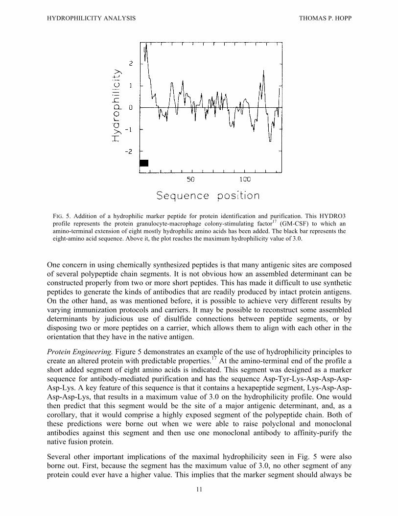
FIG. 5. Addition of a hydrophilic marker peptide for protein identification and purification. This HYDRO3 profile represents the protein granulocyte-macrophage colony-stimulating factor17 (GM-CSF) to which an amino-terminal extension of eight mostly hydrophilic amino acids has been added. The black bar represents the eight-amino acid sequence. Above it, the plot reaches the maximum hydrophilicity value of 3.0.

One concern in using chemically synthesized peptides is that many antigenic sites are composed of several polypeptide chain segments. It is not obvious how an assembled determinant can be constructed properly from two or more short peptides. This has made it difficult to use synthetic peptides to generate the kinds of antibodies that are readily produced by intact protein antigens. On the other hand, as was mentioned before, it is possible to achieve very different results by varying immunization protocols and carriers. It may be possible to reconstruct some assembled determinants by judicious use of disulfide connections between peptide segments, or by disposing two or more peptides on a carrier, which allows them to align with each other in the orientation that they have in the native antigen. Protein Engineering. Figure 5 demonstrates an example of the use of hydrophilicity principles to create an altered protein with predictable properties.17 At the amino-terminal end of the profile a short added segment of eight amino acids is indicated. This segment was designed as a marker sequence for antibody-mediated purification and has the sequence Asp-Tyr-Lys-Asp-Asp-Asp-Asp-Lys. A key feature of this sequence is that it contains a hexapeptide segment, Lys-Asp-Asp-Asp-Asp-Lys, that results in a maximum value of 3.0 on the hydrophilicity profile. One would then predict that this segment would be the site of a major antigenic determinant, and, as a corollary, that it would comprise a highly exposed segment of the polypeptide chain. Both of these predictions were borne out when we were able to raise polyclonal and monoclonal antibodies against this segment and then use one monoclonal antibody to affinity-purify the native fusion protein. Several other important implications of the maximal hydrophilicity seen in Fig. 5 were also borne out. First, because the segment has the maximum value of 3.0, no other segment of any protein could ever have a higher value. This implies that the marker segment should always be


12

exposed and express its antigenicity on any protein to which it is attached. So far, we have produced marker-fusion proteins derived by placing this sequence at the amino terminus of eight different proteins, all of which were immunoprecipitable by antimarker antibodies. Furthermore, because the marker does not fold into the protein, native biological activity is preserved. Finally, limited proteolysis tends to occur at hydrophilic peak regions. As expected, enterokinase, a protease specific for the Asp-Asp-Asp-Lys sequence, is able to rapidly cleave the marker segment to yield the authentic protein product. This further verifies the highly exposed nature of the marker segment. Summary Hydrophilicity analysis of the surface properties of proteins continues to be an important means for understanding the interactions that occur between proteins and other macromolecules. We have shown that the procedure of Hopp and Woods is useful in developing synthetic peptide immunogens and for understanding the relationship of protein sequence and folding to the interactions between macromolecules. Using a standardized procedure and the optimized hydrophilicity scale of amino acid values, it is possible to display the surface-exposed and buried portions of a polypeptide chain, as well as such features as membrane-spanning segments. Finally, an example was provided to show that hydrophilicity analysis has a place in protein engineering, allowing the creation of new surface segments with predictable properties. REFERENCES 1 T. P. Hopp and K. R. Woods, Proc. Natl. Acad. Sci. U.S.A. 78, 3824 (1981). 2 T. P. Hopp, J. Immunol. Methods 88, 1 (1986). 3 J. Kyte and R. F. Doolittle, J. Mol. Biol. 157, 105 (1982). 4 R. M. Sweet and D. Eisenberg, J. Mol. Biol. 171, 479 (1983). 5 P. Y. Chou and G. D. Fasman, Adv. Enzymol. 47, 45 (1978). 6 J. Garnier, D. J. Osguthorpe, and B. Robson, J. Mol. Biol. 120, 97 (1978). 7 Y. Nozaki and C. Tanford, J. Biol. Chem. 246, 2211 (1971). 8 T. P. Hopp, Annali Sclavo 1(2), 47 (1984). 9 P. M. Colman, J. N. Varghese, and W. G. Laver, Nature (London) 303, 41 (1983). 10 P. M. Colman, W. G. Laver, J. N. Varghese, A. T. Baker, P. A. Tulloch, G. M. Air, and R. G. Webster, Nature

(London) 326, 358 (1987). 11 S. McMillan, M. V. Seiden, R. A. Houghten, B. Clevinger, J. M. Davie, and R. A. Lerner, Cell (Cambridge,

Mass.) 35, 859 (1983). 12 A. G. Amit, R. A. Mariuzza, S. E. V. Phillips, and R. J. Poljak, Nature (London) 313, 156 (1985). 13 S. Sheriff, E. W. Silverton, E. A. Padlan, G. H. Cohen, S. J. Smith-Gill, B. C. Finzel, and D. R. Davies, Proc.

Natl. Acad. Sci. U.S.A. 84, 8075 (1987). 14 T. P. Hopp, Protides Biol. Fluids 34, 59 (1986). 15 R. A. Lerner, N. Green, H. Alexander, F. T. Liu, J. G. Sutcliffe, and T. M. Shinnick, Proc. Natl. Acad. Sci. U.S.A.

78, 3403 (1981). 16 T. P. Hopp, Mol. Immunol. 21, 13 (1984). 17 T. P. Hopp, K. S. Prickett, V. L. Price, R. T. Libby, C. J. March, D. P. Cerretti, D. L. Urdal, and P. J. Conlon,

BioTechnology 6, 1204 (1988).

Use of Hydrophilicity Plotting Procedures to Identify ... · Charged residues are often involved in...

Documents

Transcript of Use of Hydrophilicity Plotting Procedures to Identify ... · Charged residues are often involved in...