Use of ADCPs for suspended sediment transport monitoring...

RESEARCH ARTICLE10.1002/2015WR017348

Use of ADCPs for suspended sediment transport monitoring:An empirical approachJ. G. Venditti1, M. Church2, M. E. Attard1, and D. Haught1

1Department of Geography, Simon Fraser University, Burnaby, British Columbia, Canada, 2Department of Geography, TheUniversity of British Columbia, Vancouver, British Columbia, Canada

Abstract A horizontally mounted 300 kHz acoustic Doppler current profiler was deployed in Fraser Riverat Mission, British Columbia, to test its capability to detect size-classified concentration of suspended sedi-ment. Bottle samples in-beam provide a direct calibration of the hADCP signals. We also deployed a600 kHz vertically mounted ADCP from a boat in combination with bottle samples. Fraser River at Mission is525 m wide with moderate suspended sediment concentration (up to 350 mg L21 in our measurements,mostly silt), and a modest sand load only at high flows. We use an entirely empirical approach to calculatethe sediment load using ADCPs to test the reliability of acoustic methods when assumptions embedded inthe sonar equation about the relation between suspended sediment size and concentration, and acousticsignals are violated. vADCP calibration using matched individual bottle samples and acoustic backscatterdeparted from the expected theoretical relation. Calibration using depth-averaged sediment concentrationand acoustic backscatter more closely matched theoretical expectations, but varied through the season.hADCP calibrations conformed with theoretical expectations and did not exhibit seasonal variation. Silt andsand were successfully discriminated; however, silt dominates the correlations. We found no coherent rela-tion between acoustic attenuation and silt concentration. In-beam results are extended by correlation toestimate mean sediment concentration and total suspended flux in the entire channel: this auxiliary correla-tion cancels any calibration bias and permits monitoring of size-classified suspended sediment in absenceof detailed information of sediment grain-size distribution.

1. Introduction

Suspended sediment concentration in water bodies has traditionally been determined by bottle or pumpsampling and subsequent laboratory analysis of filtered solids content. The physical sample provides adefinitive indication of sediment concentration and size, but its acquisition and analysis are laborious proce-dures that do not permit high-resolution measurement, either spatially or temporally (see Gray and Landers[2013] for a recent review of traditional measurements based on the widely adopted practices of the UnitedStates Geological Survey). Automatic pump samplers may improve temporal resolution to some degree, butdo not improve important spatial resolution, and still require substantial attention and labor.

The application of suspended sediment rating curves may to some extent overcome the temporal limitationof measurements, but suspended sediment concentration varies substantially with variable sediment supplyto the water body so that rating curves are subject to significant errors [Walling, 1977]. Optical instrumentshave been developed to continuously sense suspended sediment concentration at-a-point by measuringlight transmission or backscatter, but the response depends on grain size and is a nonlinear function of con-centration [Downing, 1983]. More problematic is that the sensing elements of these instruments are subjectto fouling, necessitating frequent maintenance [Hamilton et al., 1998], often yielding only a few days’ datain biologically productive environments [Gartner, 2004].

Over the past two decades, the development of hydroacoustic instruments (Acoustic Doppler Current Pro-filers, hereafter ‘‘ADCP’’) for measuring water velocity by detecting acoustic energy backscattered from par-ticulate matter in the water column has permitted the detection of suspended sediment with very hightemporal resolution and, potentially, high spatial resolution. It is also a substantial advantage for sedimentflux estimation that these instruments can return data of both velocity and sediment concentration. Thetheory that underlies the application of acoustic transducers to measure suspended sediment is summar-ized by Thorne and Hanes [2002] and, more recently, by Thorne and Hurther [2014].

Key Points:� ADCP calibrations for suspended

sediment conform with acoustictheory� Sand and silt both correlate with

acoustic backscatter� Auxiliary relations extend results to

full-channel transport

Correspondence to:M. Church,[email protected]

Citation:Venditti, J. G., M. Church, M. E. Attard,and D. Haught (2016), Use of ADCPsfor suspended sediment transportmonitoring: An empirical approach,Water Resour. Res., 52, 2715–2736,doi:10.1002/2015WR017348.

Received 3 APR 2015

Accepted 7 MAR 2016

Accepted article online 12 MAR 2016

Published online 8 APR 2016

VC 2016. American Geophysical Union.

All Rights Reserved.

VENDITTI ET AL. ADCPS FOR SUSPENDED SEDIMENT MONITORING 2715

Water Resources Research

PUBLICATIONS

http://dx.doi.org/10.1002/2015WR017348

http://onlinelibrary.wiley.com/journal/10.1002/(ISSN)1944-7973/

http://publications.agu.org/

Combining equations given in Thorne and Hanes [2002], the foundational sonar equation can be written inlogarithmic form as

RL5SL2ðSP1ATÞ110 log 10Mqs

� �110 log 10 ff 2 3

16scas

0:96kat

� �2( )

(1)

wherein RL is reverberation level (i.e., the signal recorded by the ADCP), SL is source level (outgoing signal),SP is the beam spreading loss, AT is the signal attenuation loss, M is sediment mass concentration, and qs issediment density. The last term is the target strength, TS, which depends on ff, the form function, sc, thepulse length (pulse time 3 pulse celerity), as, the sediment grain radius, k, the acoustic wave number, andat, the transducer radius. The form function represents the cross section of the particle that is backscatteringacoustic energy, which varies with particle diameter and shape. Combining SL, which is constant for a trans-ducer, and the target strength term in equation (1), which is a constant for a given particle size and ADCP,into a constant Kt, the sonar equation becomes, with some rearrangement

log 10Mqs

� �50:1ðRL12TLÞ20:1Kt (2)

with 2TL 5 SP 1 AT denoting the two-way transmission loss [Wright et al., 2010]. The term (RL 1 2TL) isthe adjusted backscatter measured by the transducer, corrected for transmission losses along thebeam path. Linear regression between backscatter and the logarithm of volumetric sediment concen-tration should, then, theoretically yield a slope of 0.1 and an intercept of 0.1Kt [Gartner, 2004; Wrightet al., 2010]. Correction of RL (which is what is measured by the transducer) for two-way transmissionlosses can be estimated from

2TL520log 10ðrÞ12af r12asr (3)

wherein af and as are the fluid and sediment attenuation coefficients [Wright et al., 2010] and r is the dis-tance from the transducer, with further correction in the near field. Theoretical expressions for the attenua-tion coefficients involve infinite series, so they are commonly estimated from empirical relations (see reviewin Flammer [1962]; also our equations (7) and (8)).

There has been extensive research-focused application of the sonar equation and acoustic signals topredict mass concentration and grain size of particle suspensions: reviews of early work are given byHay and Sheng [1992] and by Thorne and Hanes [2002]. Much of this research has been laboratorybased and has provided the basis to invert acoustic signals to estimate suspended sediment concen-tration and grain size for sand-sized particles [cf. Hay, 1991; Hay and Sheng, 1992; Crawford and Hay,1993; Thorne et al., 1993; Thorne and Hardcastle, 1997; Thosteson and Hanes, 1998; Thorne and Hanes,2002; Thorne and Buckingham, 2004; Moate and Thorne, 2009, 2013; Moore and Hay, 2009; Thorneet al., 2010; MacDonald et al., 2013]. The primary focus of this work has been to define expressions forthe scattering properties of the particle and the attenuation characteristics of the scatterers. Itemerges—as is implicit in equation (1)—that both acoustic scatterance and attenuation depend onsediment size and mass concentration of the scatterers. Without prior knowledge of those properties,inversions for sediment concentration from acoustic backscatter may remain unbiased only for suspen-sions of fixed size distribution and uniform concentration.

Accordingly, early applications of acoustics for sensing sediment, mostly in ocean and estuarine environ-ments (summarized by Hay and Sheng [1992] and Thorne and Hanes [2002]), used custom-designed instru-ments operating at multiple frequencies of order 1 mHz to obtain observations of suspended sedimentconcentration over short ranges within which sediment properties remained essentially constant. The morerecent proliferation of commercially available, single-frequency, downward-looking ADCPs (vADCPs) hasextended the range of observations that can be obtained to the whole water column. vADCPs are increas-ingly used in examinations of sediment dynamics in estuaries [e.g., Thevenot and Kraus, 1993; Hill et al.,2003; Gartner, 2004; Wall et al., 2006, 2008; Wargo and Styles, 2007; Defendi et al., 2010; Sassi et al., 2012;Bradley et al., 2013] and rivers [e.g., Reichel and Nachtnebel, 1994; Holdaway et al., 1999; Filizola and Guyot,2004; Kostaschuk et al., 2005; Jugaru Tiron et al., 2009; Szupiany et al., 2009; Shugar et al., 2010; Sassi et al.,2013a,b; Guerrero et al., 2013; Tiron Dutu et al., 2014]. In these environments, sediment properties varysignificantly.

Water Resources Research 10.1002/2015WR017348


Conventional vADCPs still require supervised deployment, which limits their use as monitoring instruments,though much useful information might be recovered in the course of routine hydrometric measurements.However, the development of horizontally mounted ADCPs (hADCPs) for velocity-index discharge measure-ments permits a temporally continuous and spatially extended index measurement to be gained of passingsuspended sediment in rivers without continuous supervision. Arrays of hADCPs to measure fluvial sus-pended sediment concentration in a river cross section (or portion thereof) have been deployed by Toppinget al. [2007] in the Colorado River [see also Wright et al., 2010], by Moore et al. [2011] in the Rhone, Saone,and Isere Rivers (France) [see also Moore et al., 2013], and by Wood and Teasdale [2013] in the Clearwaterand Snake Rivers (USA). Topping et al. [2007], building on the work of Flammer [1962], identified two acous-tic size classes: a finer size class (silt/clay), in which increasing concentration results in greater attenuation ofsound due to viscous losses (see Moore et al. [2013] for sample attenuation curves), and a coarser size class,corresponding to sand, that results in increased backscattering of sound. They correlated the acoustic sig-nals against velocity-weighted, cross-section-averaged sediment concentrations derived from depth-integrated sampling. Correlations were developed between the silt-clay concentrations and the hADCP sig-nal attenuation and between sand and the backscatter, yielding predictions of sediment concentration spe-cific to each grain-size class and opening the way to obtain size-classified information from a singleinstrument of fixed frequency. But earlier investigators have successfully correlated silt concentration withacoustic backscatter [e.g., Hoitink and Hoekstra, 2005; see also Wood and Teasdale, 2013].

Most of the exercises with vADCPs have sought correlations between acoustic backscatter and depth-integrated suspended sediment concentration (that is, profile-average SSC), but Wall et al. [2006] correlatedthe signals from individual ADCP bins (essentially, fixed depths) with collocated point-integrated SSC, usingthe average of four ADCP beams to gain a measure of local spatial averaging. Sassi et al. [2012, 2013b] alsoemployed point-integrated samples. They used the measured backscatter profile and the samples to calcu-late sediment scattering attenuation due to mass concentration. Viscous attenuation and scattering attenu-ation due to sediment size variation along the acoustic beam were assumed to be negligible. AmonghADCP users, Topping et al. [2007] and Wood and Teasdale [2013] sought their results by correlatingobserved backscatter with the depth-integrated mean sediment concentration in the river. Moore et al.[2011] correlated hADCP signal returns with the data of an optical backscatter instrument; direct sedimentsamples were taken to calibrate the optical instrument and for grain-size confirmation. In this case, then,one index signal was used to investigate the consistency of another.

The field applications described above come face to face with constraints posed by the sonar equation,which generally limit the possibility to obtain theoretically strict estimates of suspended sediment concen-tration and size by acoustic means [Sassi et al., 2012; Hanes, 2013]. While equation (1) is specified for an indi-vidual grain size, in a natural water column, one always senses a range of sizes which, furthermore, usuallyvary along the beam vertically and, potentially, across stream. Correlation of the acoustic signal with spa-tially integrated measures of SSC directly addresses the objective of measuring suspended sediment con-centration but does not constitute a critical test of acoustic principles as the basis for the method. It issimply an empirical correlation based on the sonar principle and, since the instruments view only arestricted sample of the water column, its success relies on there being a consistent distribution of sus-pended sediment throughout the water body. Most prior investigations in natural water bodies haveassumed a correlation between acoustic backscatter and some bulk measure of sediment concentrationwithout critical examination of these assumptions.

There has not yet been a direct comparison of primary hADCP signal returns with collocated conventionalbottle or pump sampling techniques and, to our knowledge, only the work of Wall et al. [2006] and Sassiet al. [2012] has achieved this standard of investigation for vADCPs. In this paper, we seek to advance thebasis for routine monitoring of suspended sediment by directly calibrating the ADCPs using physical sedi-ment samples taken directly in the beam of the instrument to provide a test of the robustness of empiricalcorrelations based on the sonar equation. Further, we extend our observations to study the correlationbetween both vADCP and hADCP observations and measures of mean sediment concentration in the entirewater column to predict sediment flux in the river.

Many of the rivers in which ADCPs have been deployed to monitor sediment fluxes are characterized byhigh sediment loads. The Colorado River site has sediment concentrations up to 20,000 mg L21, of which3000 mg L21 is sand [Topping et al., 2007] (hADCP). The sites in the French Rivers are also characterized by



high sediment concentrations, up to 8000 mg L21 during high flows (hADCP; S. A. Moore, Monitoring flowand fluxes of suspended sediment in rivers using side-looking acoustic Doppler current profilers, unpub-lished PhD dissertation, University of Grenoble, 2011) most of which is silt-clay-sized sediment. In contrast,in the Hudson estuary [Wall et al., 2006, 2008] (vADCP), SSC did not exceed 100 mg L21, and in the Clear-water and Snake Rivers [Wood and Teasdale, 2013] (hADCP) concentrations remained below 180 and500 mg L21, respectively. In these conditions, sediment-associated beam attenuation may not pose a signif-icant problem. We deployed a shore-mounted 300 kHz hADCP in Fraser River at Mission, British Columbia(Figure 1), where sediment concentrations are intermediate between the extremes previously studied,approaching but rarely exceeding 1000 mg L21 while our measurements did not exceed 350 mg L21.Although a significant portion during high flows is sand, the suspended sediment load is dominantly silt[McLean et al., 1999].

Fraser River is �525 m wide at Mission, so we chose a 300 kHz instrument for its superior range. Wealso made periodic observations with a boat-mounted 600 kHz vADCP. Our work is distinguished fromthe work with hADCPs of Topping et al. [2007], Moore (unpublished PhD dissertation, 2011), and Woodand Teasdale [2013], in that we made direct measurements of sediment concentration and grain sizeusing conventional bottle sampling in the acoustic beam. This allowed us to develop a formal calibrationof the ADCP instrument signals with reference to the sonar equation in the manner of Wall et al. [2006,2008] for a vADCP. The goal of our work is to determine whether we can calculate suspended sedimentfluxes accurately in a river without embedding the analysis in all the assumptions implicit in the sonarequation. We seek to answer the following questions: (i) How do field-based calibrations of ADCP signalsagainst conventional bottle-sample measurements of SSC compare to sonar theory? (ii) What is the mostappropriate methodology to calculate sediment loads from a calibrated ADCP in light of the limitationsposed by sonar theory? We thereby hope to critically test an empirical basis for hydroacoustic detectionof suspended sediment in rivers and estuaries, where significant gradients in suspended sediment prop-erties are the rule. As noted, we extend our results to present consistent means to estimate the sedi-ment flux in the entire channel.

2. Methods

2.1. Study SiteFraser River at Mission drains 228,000 km2 of the humid British Columbia Coast Mountains, subhumid inte-rior plateaux, and the Columbia and Rocky Mountains. The annual hydrograph is dominated by the springsnowmelt freshet, with high flows occurring from late May until early July, and an extended recessionthrough the rest of the year with minor rises due to autumn rainstorms. One has, in effect, a single eventhydrograph at annual scale. Mean annual flood is 9790 m3 s21. The sediment load, averaging 17 3 106

tonnes per annum (on the basis of 1966–1986 measurements by the Water Survey of Canada (WSC)), iscomposed mainly of fine sand (<180 mm), silt and subordinate clay derived from the erosion of Quaternarysediments along the length of the river. On average, 18% of the annual suspended sediment load issand> 180 mm [McLean et al., 1999], all of which is transported during the freshet. The river bed at Missionis composed of sand (median diameter �380 mm) [Attard et al., 2014] that contributes intermittently sus-pended material and a bedload component. The bed is relatively flat at the study site but is covered withdunes in the upstream reach with amplitudes of order 1 m during flood.

The observation section is located 240 m upstream from the Mission water level gauge (WSC Stn.08MH024) and the Mission railway bridge (Figure 1), from which the WSC measurements were taken. Riverwidth here at mean annual flood is 540 m, declining to 520 m at mean flow stage. The river is tidally influ-enced at this point (85 km from the mouth at Sand Heads): during freshet the tidal variation is only a fewcentimeters but it may exceed one meter during winter high tides. The effect on velocity, however, remainssignificant at the highest flows as the river is subject to a backwater effect on rising tide. This semidiurnalvariation is an additional reason to establish a system of automated continuous recording of suspendedsediment concentration and flux. The seasonally reliable variation in flow and suspended sediment contentmakes the site ideal for exploratory investigation of acoustic instruments for detection of suspendedsediment.



2.2. Instrument DeploymentA 300 kHz (exact frequency 307.2 kHz) Teledyne RD ChannelMasterVR hADCP was mounted on the MissionHarbour dock (Figure 1) on the right bank of the river. It was fixed at 20.9 m geodetic datum and tilteddown at 1.28 in order to sample the full water column and to avoid interference from the water surface. ThehADCP has a beam spread of 2.28; the consequent beam projection is shown in Figure 2. The instrument

was set to collect data in128 bins each of 2 m widthso that, with a 3 m blankingdistance, its theoreticalrange extended 259 m intothe channel—that is, abouthalfway across. Data weredownloaded at approxi-mately 0.2 Hz to a com-puter mounted on thedock. Data collection com-menced on 12 April 2010and was continuous until19 August except for apower outage on 26 June.From 19 August until 3November, data were col-lected intermittently sincethe shortening days did notpermit the solar panels thatpowered the installation togenerate sufficient energyfor continuous operation.

Profile 1 Profile 2 Profile 3 Profile 4 Profile 5

-15

-10

-5

0

5

10

0 100 200 300 400 500

Elev

atio

n re

lativ

e to

geo

detic

dat

um (m

)

Distance across the channel (m)

Figure 2. Ensonified areas of the 300 kHz horizontal ADCP (blue) and the 600 kHz vertical ADCP(red is all four beams and green is the forward looking beam #3). Solid black lines are the bedtopography immediately upstream and downstream surveyed in 2008 by Public Works Canada.Crosses mark the positions of the bottle-sampled profiles and vADCP observations. The longdashed line is the water level at Mission when the discharge at Hope was �5000 m3/s(�6060 m3/s at Mission) in 2010. The short dashed line is the water level at Mission during thepeak 2010 discharge (�7500 m3/s).

Figure 1. Bed topography of Mission Reach and Hatzic bend showing the location of the 300 kHz hADCP and the study cross section. Insetshows locations of bottle sampling and 600 kHz vertical ADCP profiles (numbered 1–5). Bed topography is from Public Works Canada crosssections measured every 100 m along the channel in 2008. Main imagery from 1995 airphotos. Inset imagery from Google Earth accessed6 July 2013.



A 600 kHz (exact frequency 614.4 kHz) Teledyne RD Workhorse Rio GrandeVR vADCP was deployed from a6 m launch to collect vertical profiles of velocity and suspended sediment concentration at five positionsacross the channel (Figure 2). Data were recorded at approximately 1 Hz to an onboard computer. A TrimbleGPS Rover operated in RTK mode was used for positioning. Sampling dates are listed in Figure 4.

Bottle samples were taken in the beam of the hADCP at eight fixed distances from the instrument between27.5 and 300 m with a P63 suspended sediment sampler. The P63 [Gray and Landers, 2013] is a point-integrating sampler that collects an isokinetic sample in a 950 mL bottle. Sampling times were varied toachieve samples that typically varied from 700 to 850 mL. Bottle samples were also collected at the fivevADCP profile positions for calibration purposes and to calculate the total sediment flux in the channelindependently of the ADCP observations (see Attard et al. [2014] for analysis of bottle sampled sedimentflux). The P63 was deployed from the opposite side of the launch (separation from the acoustic signalapproximately 2 m) and samples were taken at 0.1, 0.2, 0.4, 0.6, and 0.8 of full depth, with minor variationson 16 April (four positions in profile) and 28 June (Profile 5 not collected) due to instrument failures.

2.3. Data ProcessingThe use of hydroacoustic instruments to measure suspended sediment is based on the sonar equation inthe form of equation (2), extended by an empirical relation between suspended sediment concentrationand acoustic backscatter adjusted for two-way transmission losses. ADCPs return a measure of backscatter(RL) as the echo intensity (EI) in counts, which is converted to RL in decibel units as:

RL5sf 3EI (4)

in which sf is an instrument-specific scale factor. The measured backscatter is corrected for two-way trans-mission losses associated with fluid attenuation by applying the sonar equation [Urick, 1975] to calculatethe fluid-corrected backscatter (FCB) from

FCB5RL120 log10 rð Þ12af (5)

wherein r is distance along the acoustic beam. This has the effect of replacing the backscatter lost to fluidattenuation with distance from the transducer. In the ‘‘near field,’’ the second term becomes 20log10(rw)wherein w is an additional correction. Wall et al. [2006] determined that this factor makes of order 1% differ-ence to the final result, so we have ignored it. We have also ignored several instrument-specific constantsbecause they affect only the magnitude of the signal, but not its relative variability [cf. Deines, 1999; Sassiet al., 2012]. The water absorption coefficient, af, is computed [Schulkin and Marsh, 1962] for zero salinity from

af 58:68633:3831026 f 2

fT(6a)

fT 521:9310 62 1520T1273ð Þ (6b)

wherein f is the frequency of the ADCP and T is the water temperature in degrees Celsius.

In flows with high sediment concentrations, corrections for two-way transmissions losses associated withsediment in suspension may also be needed. This can be accomplished by calculating the sediment cor-rected backscatter as

SCB5FCB12asr (7)

where as is a sediment attenuation coefficient which can be calculated from theory [Hay, 1991], semitheoreti-cally [e.g., Sassi et al., 2012] or empirically [Topping et al., 2007; Wright et al., 2010]. This correction has theeffect of replacing the backscatter lost to viscous and scattering attenuation with distance from the trans-ducer. The theoretically strict calculation requires the grain-size distribution and mass concentration of par-ticles in suspension [e.g., Moore et al., 2013; Moate and Thorne, 2013]. If the size or mass concentration variesalong the acoustic beam or through time, that variation must also be known. The consequent need for con-tinuous physical sampling would defeat the purpose of the acoustic observations in a long-term monitoringprogram.

Sassi et al. [2012] introduced a semitheoretical method to account for attenuation that simplifies the datarequirements somewhat by requiring only mass concentration near the transducer, where sediment



attenuation is assumed to be negligible, and somewhere else along the acoustic beam where scatteringattenuation is assumed to occur due to the gradient in mass concentration. Viscous attenuation by sedi-ment and scattering attenuation that may occur due to a gradient in sediment size is ignored. This methodcannot be successfully applied to our data because viscous sediment attenuation is not negligible for thecombination of suspended sediment sizes in the Fraser and our acoustic frequencies (Figure 3). Further-more, there is a substantial grain-size gradient (see below) that can contribute to the scattering attenuation.

An empirical approach is somewhat simpler in that as is calculated as

as5212

SFCB;r (8)

where SFCB;r is the slope of the least squares linear regression between FCB and r [Topping et al., 2007; Wrightet al., 2010] (equation (8) is the derivative, d/dr, of equation (7), under the assumption that sediment con-centration is independent of r). However, its calculation assumes spatially uniform sediment properties suchthat SFCB;r is negative. In the presence of physical gradients in size and mass concentration, SFCB;r dependson sediment attenuation and those gradients. The requirement for uniform mass concentration and sedi-ment properties along the acoustic beam can be coincidentally met in some hADCP deployments, but

rarely in vADCP deployments.

We implemented the empirical sedi-ment correction method for thehADCP because the underlyingassumptions could be met. A fortunateconsequence of selecting a 300 kHzinstrument for maximum range is thatthe instrument has minimum sensitiv-ity to both viscous and scattering sedi-ment attenuation for sedimentssuspended in Fraser River (Figure 3).This means that the sediment correc-tions are small. Some care needs to betaken in calculating SFCB;r becauseobstructions within the ensonified vol-ume of flow and signal decay beyondthe specified operating range of theADCP will affect the FCB-r relation, but

0.00

0.01

0.02

0.03

0.04

0.05

0.06

0.07

0.08

0.09

0.10

0.00

0.01

0.02

0.03

0.04

0.05

0.06

0.07

0.08

0.09

0.10

0.01 0.1 1 10 100 1000 10000 100000 1000000

F rac

on in

sus

pens

ion

Aen

uaon

coe

ffici

ent

(m2 /

kg)

D50 (microns)

Sca ering 600

Sca ering 300

Viscous 600

Viscous 300

April 16 2010

May 19 2010

May 28 2010

June 7 2010

June 28 2010

August 4 2010

Figure 3. Viscous and scattering attenuation coefficients plotted as a function of median grain size for the 300 and 600 kHz transducers.Also plotted are the grain-size distributions from each sampling campaign for Profile 3 at 0.6d.

00.10.20.30.40.50.60.70.80.9

1

60 70 80 90 100 110

z/d

Fluid Corrected Backscatter (dB)

16-Apr-10

18-May-10

28-May-10

8-Jun-10

28-Jun-10

4-Aug-10

Figure 4. Typical vertical profiles of fluid corrected backscatter from the 600 kHzvADCP at Profile 3. Profile 4 is substituted for Profile 3 on 16 April 2010 because ofan instrument failure.



not necessarily the recorded velocity. This correction reduced hADCP backscatter to a common integralvalue, obviating the possibility to make bin-by-bin estimates of sediment concentration.

Application of this empirical method to correct the vADCP data is not possible due to the gradients in massconcentration and grain size. Removing the vertical gradient in the same manner as the hADCP would havethe effect of rotating the profile about the first point not affected by near-field effects. SCB would be lessthan the measured backscatter. We applied the Sassi et al. [2012] method to our 600 kHz records and foundnegative values of as along the entire profile, so we did not pursue this method further. We therefore focusfurther analysis on the bin-by-bin and depth-averaged FCB. Like the 300 kHz instrument, the 600 kHz vADCPhas minimum sensitivity to both viscous and scattering attenuation for the majority of suspendedsediments in the Fraser River (Figure 3). This suggests that the necessary correction is small and can prob-ably be ignored, an assumption we can test by comparison of our FCB observations with theoreticalexpectations.

In order to calculate suspended sediment concentration (SSC) from FCB, we used the following relation, dueto Gartner [2004]:

SSC510 a�FCB1bð Þ (9a)

wherein a and b are the slope and intercept of a least squares regression, respectively. We investigated theseparate sand and silt-clay calibrations with FCB and investigated the hADCP calibrations with SSC com-puted from SCB as

SSC510 a�SCB1bð Þ (9b)

Topping et al. [2007] and Wright et al. [2010] have argued that FCB can be related to total sediment concen-tration, SCB to sand concentration, and silt-clay concentrations to as. We also studied the correlationbetween silt-clay concentration and as but, finding no significant result, we did not pursue this relation.

Data were correlated using linear least squares under logarithmic transformation of SSC. Because residualsare not normally distributed, back-transform bias was eliminated to obtain equations (9) using the ‘‘smear-ing’’ method [Duan, 1983; Newman, 1993]. The underlying calibrations were obtained as reduced major axisfunctional relations, which assume that the error ratio of the variables is equal to the ratio of their sums ofsquared departures from the mean, and is the maximum likelihood estimate of the error ratio when it is infact unknown [see Mark and Church, 1977].

3. ADCP Calibrations

3.1. The 600 kHz vADCPFigure 4 displays fluid-corrected backscatter from the vADCP in the center of the channel. Backscatterincreased toward the bed, as expected, and the backscatter intensity varied through the season in concertwith flow and suspended sediment concentration. Calibrations were developed between the variously cor-rected acoustic signals and sampled sediment mass concentration for the total and component concentra-tions. In the calibration exercise, vADCP data immediately adjacent to the surface and the bed that wereobviously perturbed by the presence of the boundaries were ignored. This entailed deleting data aboveand below the infection points in Figure 4.

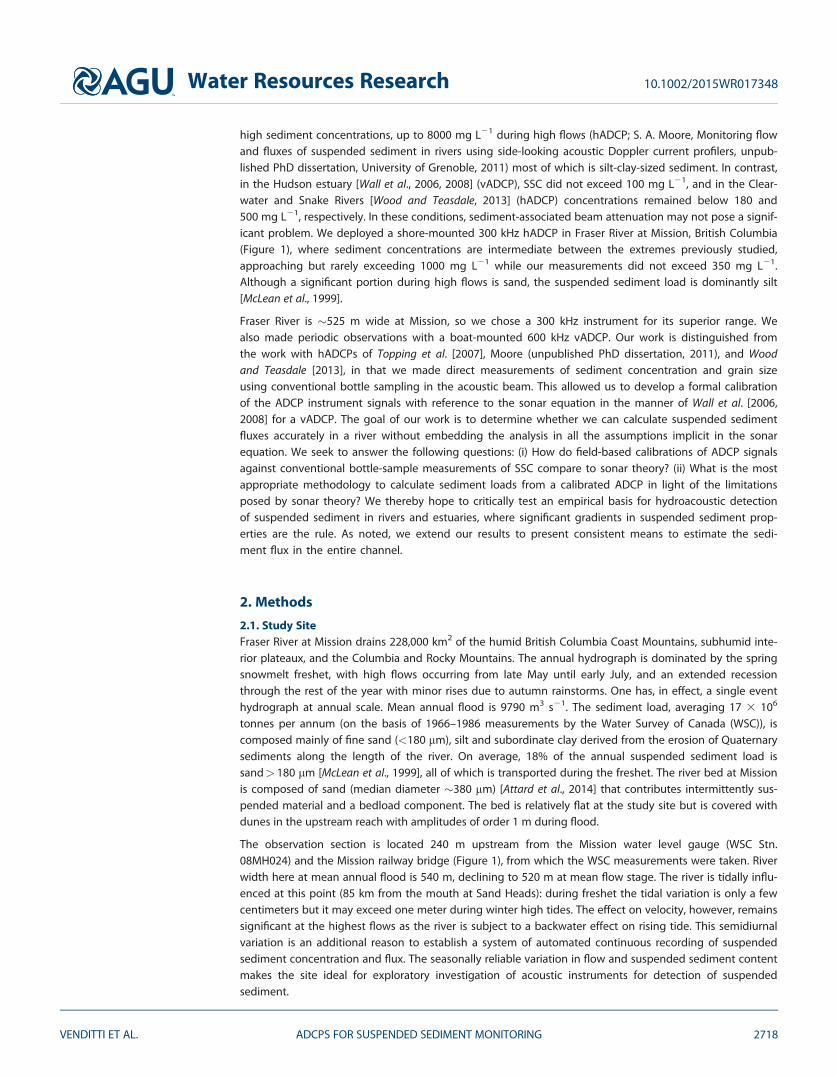
The most direct relation between the acoustic signal and SSC is obtained by correlation between the physi-cal sample and the acoustic signal from the vADCP profile bin in (or very near) which the physical sedimentsample was collected (bin-by-bin calibration), which we obtain for FCB. We also obtained the correlationbetween the depth-averaged FCB and SSC—’’indirect’’ results, but convenient for prediction of profile-average SSC. Figure 5 displays bin-by-bin and depth-averaged calibrations. The bin-by-bin results are basedon the instrument signal observed in the profile bin at the depth at which the physical sample was taken,but there remains the 2 m lateral distance between the two observations. All samples were used, normallyyielding five calibration points per profile.

The depth-averaged SSC from bottle sampling was calculated as



<SSC> 5X

ci di ui=X

di ui (10)

in which <SSC> is the profile-averaged SSC (angle brackets indicate a depth-average), ci is a sample value,di is the height of the water column that the sample represents, and ui is the velocity from the correspond-ing ADCP bin, representing the mean velocity for the corresponding depth range. The depth-averaged SSCfrom the vADCP is calculated in similar fashion with ci derived from the ADCP calibration.

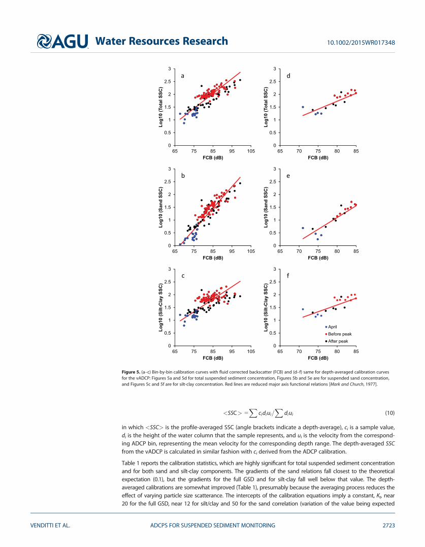
Table 1 reports the calibration statistics, which are highly significant for total suspended sediment concentrationand for both sand and silt-clay components. The gradients of the sand relations fall closest to the theoreticalexpectation (0.1), but the gradients for the full GSD and for silt-clay fall well below that value. The depth-averaged calibrations are somewhat improved (Table 1), presumably because the averaging process reduces theeffect of varying particle size scatterance. The intercepts of the calibration equations imply a constant, Kt, near20 for the full GSD, near 12 for silt/clay and 50 for the sand correlation (variation of the value being expected

0

0.5

1

1.5

2

2.5

3

65 75 85 95 105

L og1

0 ( S

a nd

SSC

)

FCB (dB)

b

0

0.5

1

1.5

2

2.5

3

65 75 85 95 105

L og1

0 (S

ilt-C

l ay

SSC

)

FCB (dB)

c

0

0.5

1

1.5

2

2.5

3

65 75 85 95 105

Log1

0 (T

otal

SSC

)FCB (dB)

a

0

0.5

1

1.5

2

2.5

3

65 70 75 80 85

Log1

0 (T

o tal

SSC

)

FCB (dB)

d

0

0.5

1

1.5

2

2.5

3

65 70 75 80 85

Log1

0 (S

and

SSC

)FCB (dB)

e

0

0.5

1

1.5

2

2.5

3

65 70 75 80 85

L og1

0 (S

ilt-C

lay

SSC

)

FCB (dB)

AprilBefore peakAfter peak

f

Figure 5. (a–c) Bin-by-bin calibration curves with fluid corrected backscatter (FCB) and (d–f) same for depth-averaged calibration curvesfor the vADCP: Figures 5a and 5d for total suspended sediment concentration, Figures 5b and 5e are for suspended sand concentration,and Figures 5c and 5f are for silt-clay concentration. Red lines are reduced major axis functional relations [Mark and Church, 1977].



because it depends, amongst other factors, on the ‘‘effective grain size’’ of the sediment scatterers). It is clearthat the silt-clay fraction dominates the total GSD of suspended sediment in Fraser River (Figure 6), accountingfor the similarity of the calibrations for total GSD and for silt-clay.

We find, however, that the overall calibrations displayed above are not stable. Figure 7 shows that results froman individual sampling may remain biased. Indeed, dividing the data into subsets for the rising limb and fallinglimb of the hydrograph leads to distinct clusters of data (Figure 5) and to calibration equations with significantlydifferent slopes (0.062 versus 0.041; p< 0.05 for total SSC with FCB bin-by-bin). Before the freshet peak, sus-pended sediment concentration appears to respond with more sensitivity than after the peak. But if, instead, wegroup the low flow observations of 16 April (before the commencement of the freshet, when total suspendedsediment concentration was very low (values 10–30 mg L21) with the post-freshet observations, we find twoequations with equivalent slope but different intercepts, implying a systematically changed grain size. The pres-ence/absence of a significant suspended sand component (Figure 3) may account for the shift. The depth-averaged results appear to be more stable in this regard.

3.2. The 300 kHz Horizontal ADCPFigure 8a shows the season-long cross-stream backscatter signal (water corrected) recovered from thehADCP, which follows the seasonal pattern of streamflow, as does sediment concentration. Figure 8b showsin detail the raw and corrected signals for 28 June (the peak flow day). Both parts of the figure exhibit thesame unexpected feature: signal strength declines as expected out to 60 m, but then increases to 130 m

before beginning to decrease again. The signal also showsincreased local variation beyond 60 m. We interpret thesefeatures to indicate that the beam has encountered someunusual interference beyond 60 m. Figure 2 shows thatbed interference should be encountered only near 180 mand that water surface interference should not occur. Thebed is probably the source of interference in view of trans-ducer side-lobe effects but we remain uncertain—in anyevent, the signal appears to be spurious beyond 60 m. Thisoutcome compromises hADCP in-beam calibration meas-urements beyond that distance, consequently we confineattention to a beam-averaged calibration covering the first60 m. In this sector, relatively quiet water carries silt andfine sand with limited size variation over the season and inthe vertical (Figure 9), and a small range in concentration(Figure 10), making the accessible sampling volume rela-tively ideal for consistent hADCP sediment detection.(Buschman et al. [2012] have previously described lowcross-sectional variation in suspended sediment concentra-tion in a silt-clay dominated river.)

0

50

100

150

0 50 100 150 200

Silt-

Cla

y SS

C (m

g/L)

Total SSC (mg/L)

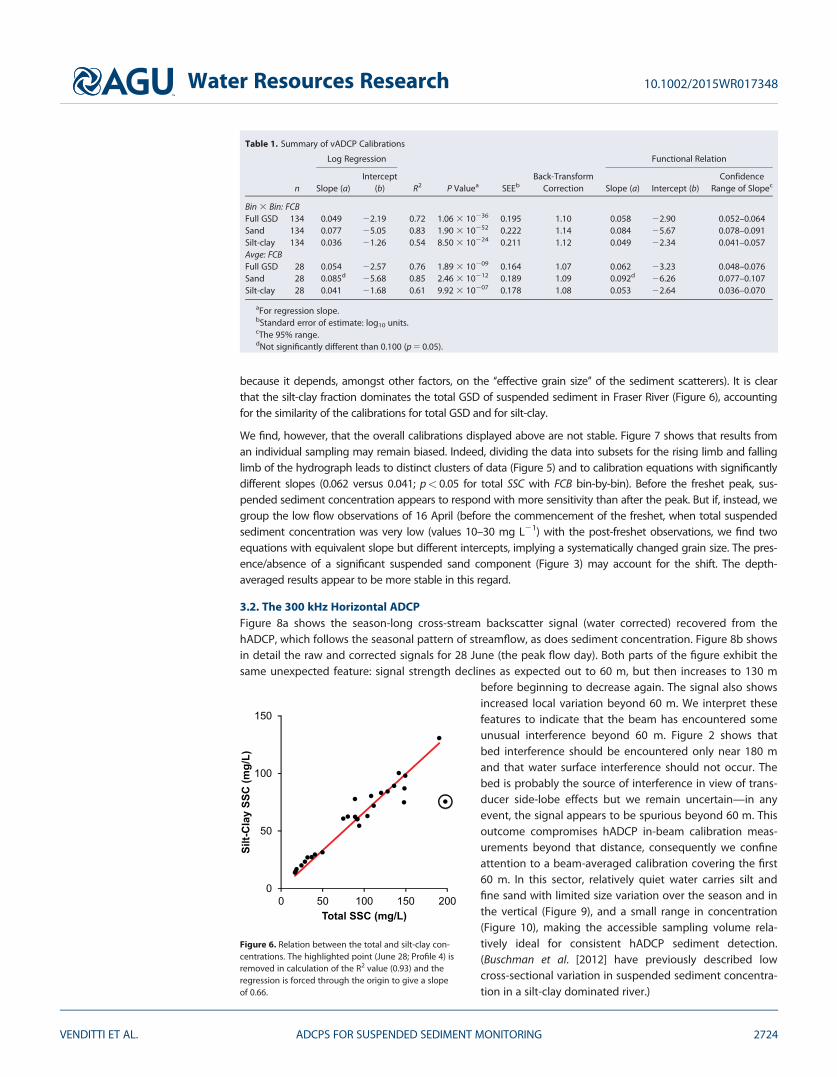
Figure 6. Relation between the total and silt-clay con-centrations. The highlighted point (June 28; Profile 4) isremoved in calculation of the R2 value (0.93) and theregression is forced through the origin to give a slopeof 0.66.

Table 1. Summary of vADCP Calibrations

n

Log Regression

R2 P Valuea SEEbBack-Transform

Correction

Functional Relation

Slope (a)Intercept

(b) Slope (a) Intercept (b)Confidence

Range of Slopec

Bin 3 Bin: FCBFull GSD 134 0.049 22.19 0.72 1.06 3 10236 0.195 1.10 0.058 22.90 0.052–0.064Sand 134 0.077 25.05 0.83 1.90 3 10252 0.222 1.14 0.084 25.67 0.078–0.091Silt-clay 134 0.036 21.26 0.54 8.50 3 10224 0.211 1.12 0.049 22.34 0.041–0.057Avge: FCBFull GSD 28 0.054 22.57 0.76 1.89 3 10209 0.164 1.07 0.062 23.23 0.048–0.076Sand 28 0.085d 25.68 0.85 2.46 3 10212 0.189 1.09 0.092d 26.26 0.077–0.107Silt-clay 28 0.041 21.68 0.61 9.92 3 10207 0.178 1.08 0.053 22.64 0.036–0.070

aFor regression slope.bStandard error of estimate: log10 units.cThe 95% range.dNot significantly different than 0.100 (p 5 0.05).



Initial plotting of the data reveals an excellent correlation save one errant datum (observations of 27 May:see Figure 11). We are uncertain why this datum plots off-trend, but we delete it from the calibration.Table 2 gives statistics of the beam-averaged correlation based on the backscatter data from the first 60 mof the cross-stream record collected in the five remaining measurement campaigns, and on an average ofthe corresponding observed SSC from in-beam bottle samples collected at 27.5, 50, and 55 m from theinstrument. The bottle sample data were averaged as

cT 5X

ci wi=X

wi (11)

in which wi is the width of channel that each sample represents.

00.10.20.30.40.50.60.70.80.9

1

0 100 200 300 400 500

z / d

Total SSC (mg/L)

00.10.20.30.40.50.60.70.80.9

1

0 100 200 300 400 500

z / d

00.10.20.30.40.50.60.70.80.9

1

0 100 200 300 400 500

z / d

00.10.20.30.40.50.60.70.80.9

1

0 100 200 300 400 500z

/ d

00.10.20.30.40.50.60.70.80.9

1

0 100 200 300 400 500

z / d

00.10.20.30.40.50.60.70.80.9

1

0 100 200 300 400 500

z / d

Total SSC (mg/L)

vADCPBottle Samples

a) April 15

c) May 27

e) June 28

b) May 18

d) June 7

f) August 4

Figure 7. Vertical profiles of measured suspended sediment concentration from the bin 3 bin calibrated vADCP and corresponding bottlesamples. Data from Profile 3, except 15 April and 7 June which are Profile 4 because either bottle or VADCP profiles were not available.



The correlations displayed in Figure 11 are very high and the gradients not significantly different than thetheoretically expected value of 0.1. Silt-clay correlates very well with backscatter and clearly controls thecorrelation with total suspended solids. There is no coherent relation between sediment attenuation andsilt-clay concentrations (Figure 12), except during peak flow (28 June) when SFCB;r is negative, indicatingthere is some attenuation of the signal at high sediment concentrations [cf. Moore et al., 2013]. At lowerflows, SFCB;r is negligibly small and varies between positive and negative values. Gradients in the FCB profileare due to variability in the shape of the measured profile. The result confirms initial expectations thatattenuation is negligibly small—an assumption underlying the adoption of equation (9a)—so FCB-correctedresults and SCB-corrected results are virtually the same (that is, removal of the residual slope has no materialeffect on the results). Kt appears to vary between 65 and 110, the high values being for sand. The correla-tions are so high that no back transform correction was applied (correlation is essentially 1.0), and the func-tional estimate coincides with the regression equation.

4. Calculation of Sediment Loads

4.1. Bottle SamplesSediment flux in each of the five profiles was calculated from bottle samples according to

qsj5X

ci ui di (12)

in which j indexes a profile, and for the channel as

Qs5X

qsjwj (13)

Details of the analysis of the bottle samples for sediment flux estimation are given in Attard et al. [2014].

Figure 8. (a) Cross-stream profiles of fluid corrected backscatter (FCB) plotted through time. (b) Profiles of measured backscatter (MB), FCB,and sediment and water-corrected backscatter (SCB) measured on 28 June 2010. The corrected plots are truncated at 60 m. Inset:expanded view of corrected plots.



4.2. Comparison of Flux Estimates:600 kHz Vertical ADCPThe sediment flux was estimated from thevADCP measurements using equations(12) and (13), but ci was derived from thevADCP bin-by-bin calibration. Using thedepth-averaged calibration, sediment fluxwas also calculated for each profile from

<qsj > 5 <SSCj ><uj > dj (14)

wherein <u> is the depth-averaged veloc-ity. Sediment flux for the channel is then

Qs5X

<qsj > wj (15)

Figure 13 compares SSC estimates derivedfrom the bin-by-bin vADCP calibration(Figure 5). The correspondence is goodbut shows some significant underes-timates at low to moderate sedimentconcentrations. Comparison with depth-averaged sediment fluxes, also shown inFigure 13, shows generally superior preci-sion, but some significant overestimateson the high flow dates. The biased resultscan be traced to variation about the meancalibration relations (Figure 5), effects ofwhich are also displayed in Figure 7.

4.3. Comparison of Flux Estimates:300 kHz Horizontal ADCPIn order to calculate suspended sedimentflux in the channel from continuoushADCP records, we must establish a corre-lation between the beam-averaged cali-bration based on measurements in thebeam, reported in Table 2, and somemeasure of sediment flux in the entirechannel. We have explored two ways ofaccomplishing this:

1. We correlate the sediment flux in thechannel (determined from integrationof the bottle samples) with fluxthrough the ensonified volume. Sedi-ment flux passing through the acous-tic cone of the hADCP is estimated as

Qsh5SSCh < uh > Ac (16)

wherein SSCh is the suspended sedi-ment concentration obtained from thebeam-averaged calibration, <uh > isthe mean velocity of the water column,averaged along the beam, and Ac is the2-D cross section of the acoustic beam

0.0

10.0

20.0

30.0

40.0

50.0

60.0

01/04 01/05 31/05 30/06 30/07 29/08

D50

(mic

rons

)

Date (dd/mm)

0.1d0.2d0.4d0.6d0.8d

0.0

10.0

20.0

30.0

40.0

50.0

60.0

70.0

80.0

90.0

01/04 01/05 31/05 30/06 30/07 29/08

D50

(mic

rons

)

Date (dd/mm)

Sand

Silt

b) Profile 2

a) Profile 1

Figure 9. Profiles of suspended sediment grain size (D50) on Profiles 1 and 2,through the season. The point for 30.06 at 0.2d on Profile 1 (in true beam)may be spurious, but points on Profile 2 (in the contaminated beam) indicatethat significant excursions in sediment grain size do occur. Data in Attardet al. [2014, Figure 8]; 0.1d is near the bed and 0.8d is near the water surface.

0

20

40

60

80

100

120

140

4/15 5/19 5/27 6/7 6/27 8/3

Dep

th-a

vera

ged

Conc

entr

aon

(mg/

L)

Date

Profile 1

Profile 2

Figure 10. Comparison of profile-average suspended sediment concentrationat Profiles 1 and 2, from bottle sampling.



Ac512

30 bins � 2mbin

� �hb (17)

wherein hb is the height of acoustic beam at60 m and 2 m/bin denotes the 2 m width ofa bin. Using this estimate, we develop a cor-relation between Qsh and sediment flux inthe channel based on bottle sample verticalprofiles, QsChan, that has the form

QsChan5aQshb (18)

where a and b are derived from leastsquares regression.

2. We relate channel-averaged SSC to SSC inthe ensonified area. A correlation is estab-lished between SSCh and the measuredchannel-averaged suspended sedimentconcentration, SSCChan, that has the form

SSCChan5aSSChb (19a)

in which a and b are, again, derived fromleast squares regression. Sediment flux isthen calculated as

QsChan5SSCChan � Q (19b)

wherein Q is the discharge from the WSCgauging station at Mission. In a relation sim-ilar to that of equation (19a), we also studythe correlation between SSCh and SSCp3, thedepth-averaged suspended sediment con-centration at Profile 3 (Figure 2), a centralprofile formerly used by the Water Survey ofCanada to obtain single-vertical bottle sam-ples as an index of suspended sediment fluxin the river. In each case, we examine rela-tions for total SSC, sand, and silt/clay.

In deriving both Qsh and SSCh, we use sum-mary mean values directly derived from

Figure 11. Along-beam-averaged hADCP calibration curves betweensediment corrected backscatter (SCB) and (a) total suspended sedimentconcentration (SSC) and (b) sand and silt concentration. Lines areregression equations: further details in text. Because of interference, theacoustic profiles are truncated at 60 m. The circled point is the errantdatum from 27 May.

Table 2. Summary of hADCP Calibrations

n Slope (a) Intercept (b) R2 P Valuea SEEb Confidence Range of Slopec

30 Bins: FCBFull GSD 5 0.098d 26.89 0.99 2.82 3 10204 0.037 0.082–0.113Sand 5 0.125d 210.0 0.95 4.64 3 10203 0.123 0.073–0.177Silt-clay 5 0.092d 26.46 0.99 2.89 3 10204 0.035 0.077–0.10730 Bins: SCBFull GSD 5 0.106d 27.63 0.99 4.50 3 10204 0.043 0.086–0.126Sand 5 0.136d 211.0 0.95 4.81 3 10203 0.124 0.079–0.193Silt-clay 5 0.100d 27.16 0.99 4.93 3 10204 0.042 0.080–0.119

aFor regression slope.bStandard error of estimate: log10 units.cThe 95% range.dNot significantly different than 0.100 (p 5 0.05).



beam-average quantities, hence covariance issues (between flow and sediment concentration) do not arise.We employ regression since the results will be used for prediction. Either method can be used to predict acontinuous record of sediment flux from the hADCP data. We seek to learn whether beam-average resultsyield unbiased estimates of the load. (The regression equation may, of course, offset systematic biasbetween the two estimates provided that bias is consistent across the range of values.) We conducted theanalysis using SCB corrected data. The regressions described in equations (18) and (19b) were establishedfor the full grain-size distribution and for the load components in log linear form (Figure 14). Table 3 sum-marizes the parameters of these relations. In Table 3, we give parameters for the median regressions: that isthe back-transformed power relations without transform bias correction. This form discounts the effect ofexcentric outliers (here particularly, the high flow points) and is adopted because of the irregular distribu-tion of the small data sets.

The correlations for the full-channel sediment flux, illustrated in Figure 14, are all strong, most R2 valuesbeing around 0.90 or above for the full grain-size distribution (Table 3). However, the full-channel correla-tions for sand in SSC-derived relations fall to 0.80. The small number of data points (n 5 6) means that theanalyses have low statistical power so that standard errors of the regression coefficients are large. However,all regression slopes for the full-channel actually cluster around the value 1.0. The value 1.0 implies simpleproportional relations between sediment load and concentration in the hADCP beam and in the river, theproportional ratio being the intercept of the relation. On this basis, Qs � 170 Qsh for the full range of sus-pended sediment, while Qs-sand � 300Qsh-sand and Qs-silt.clay � 140Qsh-silt/clay.

The proportional relations based on SSC are close to 2.0, except sand rises to 2.34, as one would expectsince most sand suspension occurs in the unensonified main flow. The correlation of SSCh with SSCp3 (n 5 5)returns R2 � 0.75 and regression slopes fall near 0.75 (though no result can be confidently declared to bestatistically different than 1.0). In this case, there is no simple proportionality between hADCP values andthose at P3. This is not surprising as P3, in the thalweg, is subject to relatively high sediment concentrationsall season, reflected in larger coefficients but a less rapid rate of adjustment with increasing flow than in theequivalent full-channel comparisons.

All the results are unbiased (Figure 15) and, apart from one set of underpredictions for total grain-size distri-bution and sand deriving from an excentric high flow datum (Figure 14), relatively precise.

4.4. The Sediment Flux RegimeFigure 16 reveals that the annual sedigraph exhibits hysteresis, with higher sediment concentration and,therefore, sediment flux on the rising limb than on the falling limb. This feature of the annual sediment loadis well known [McLean et al., 1999; Attard et al., 2014], so the result confirms that the measurements usingADCP data capture an important detail of the annual sediment load. However, the hADCP estimates predictgreater flux on the rising limb of the seasonal flood than indicated by the physical samples while at the

peak flow and on the falling limb the reverseoccurs. This results in greater hysteresis than is dis-played by the physical samples. In comparison, thevADCP estimates of sediment transport, sampled inthe same positions as the bottle samples, showgreater congruence with the physical samples andlesser hysteresis.

5. Discussion

5.1. Can we Directly Calibrate ConventionalBottle Sample Field Measurements of SSCAgainst Acoustic Signals?The sensitivity of acoustic signals to suspendedsediment concentration has been demonstrated inseveral rivers [e.g., Wall et al., 2006; Topping et al.,2007; Wright et al., 2010; Moore et al., 2011, 2013;Sassi et al., 2012; Wood and Teasdale, 2013], in

-0.04

-0.03

-0.02

-0.01

0

0.01

0.02

0 50 100 150

S FC

B,r

(dB

/m)

Silt-Clay SSC (mg/L)

AprilBefore peakAfter peak

Figure 12. Data of sediment attenuation versus silt-clay concen-tration for the hADCP; the circled point is from 28 Junemeasurements.



conditions both of a high silt/clay load and a low overall load. In comparison, the silt/clay load in FraserRiver is modest, and the preponderance is silt, while the overall load peaks at an intermediate level due tothe entrainment of sand from the bed in the higher flows. Our tests have been conducted in a substantiallydifferent environment than previous investigations and so contribute to a robust evaluation of how widelythe method might be employed.

Topping et al. [2007] and Wright et al. [2010] contrasted the response of fine (silt-clay) and coarse (sand) sus-pended material to acoustic energy, noting that fines dominantly attenuate the reflected signal whilecoarse material scatters acoustic energy. Accordingly, they suggested that suspended silt and clay

0

1

2

3

4

5

0 1 2 3 4 5

V-AD

CP

Tota

l qs

( kg/

m/ s

)

Bottle Sample Total qs (kg/m/s)

0

0.5

1

1.5

2

2.5

3

0 0.5 1 1.5 2 2.5 3V-

ADC

P Sa

n d q

s ( k

g/m

/ s)

Bottle Sample Sand qs (kg/m/s)

0

0.5

1

1.5

2

2.5

3

0 0.5 1 1.5 2 2.5 3

V-AD

CP

Silt-

clay

qs

(kg/

m/s

)

Bottle Sample Silt-clay qs (kg/m/s)

15-Apr19-May27-May7-Jun27-Jun3-Aug

0

1

2

3

4

5

0 1 2 3 4 5

V-AD

CP

Tota

l qs

(kg/

m/s

)

Bottle Sample Total qs (kg/m/s)

0

0.5

1

1.5

2

2.5

3

0 0.5 1 1.5 2 2.5 3

V -AD

CP

Sand

qs

(kg/

m/s

)

Bottle Sample Sand qs (kg/m/s)

0

0.5

1

1.5

2

2.5

3

0 0.5 1 1.5 2 2.5 3

V -AD

CP

Sil t-

clay

qs

(kg/

m/ s

)

Bottle Sample Silt-clay qs (kg/m/s)

a

b

c

d

e

f

Figure 13. Comparison of vADCP bin-by-bin calibrated (a–c) and depth-averaged (d–f) sediment fluxes. Figures 13a and 13d are for totalsuspended sediment concentration, Figures 13b and 13e are for suspended sand concentration, and Figures 13c and 13f are for silt-clayconcentration. The thick dashed lines are 650% and the thin dashed lines are 6100%.



concentration be measured via acoustic signalattenuation, while sand can be measured via acous-tic backscatter. It has been suggested [Topping et al.,2007] that this division should remain valid for sus-pended sediment concentration varying from 10 to104 mg L21. In this light, our relation of silt-clay tobackscatter appears unusual, though not withoutprecedent, and perhaps related to the dominantlycoarse silt makeup of the load and its relation toattenuation properties of our instruments (Figure 3).Considering backscatter, at 300 kHz response at 20mm (see Figure 9 for grain size) is an order of magni-tude less effective than at 200 mm. However, similarresults (that is, good correlation of silt-clay with SCB)have previously been obtained in Snake and Clear-water Rivers using 1.5 and 3.0 MHz hADCPs [Woodand Teasdale, 2013] and the coefficients obtained intheir equations are similar to those we haveobtained. Our calibrations for total SSC and for sandconcentration are highly significant but in view ofthe dominance of silt in the suspended load of theriver, the calibration of total SSC mainly depends onthe coherent relation obtained for silt-clay.

The bin-by-bin correlation derived from the vADCPis slightly poorer than the averaged results, possiblybeing degraded by variation due to the imperfectcollocation of samples and the ADCP profiles, butalso by the significant variation in grain size andconcentration in the vertical profile. While the slopeof the sand relation approximately conforms withtheory, the slopes for total SSC and silt-clay departfrom the theoretically expected value of 0.1. Thebeam-averaged procedure yields the more robustresults. Bin-by-bin correlation must contend with thepossibility that the grain size of suspended sedimentmay vary from bin to bin in a systematic way, whichmay contribute a portion of variance to the

1

10

100

1000

0.01 0.1 1 10

Qs

( kg/

s)

Qh (kg/s)

SandFull GSDSilt-Clay

1

10

100

0.1 1 10 100 1000

SSC

P3(m

g/L )

SSCh (mg/L)

1

10

100

1 10 100 1000

SSC

chan

(mg/

L)

SSCh (mg/L)

a

b

c

Figure 14. (a) Relations between sediment flux in the 300 kHzhADCP cone derived from the sediment corrected backscattercalibration (Qh) and sediment flux in the channel (Qs), (b) SSC inthe 300 kHz hADCP cone (SSCh) and SSC in the channel (SSCchan),and (c) SSCh and SSC at Profile 3 (SSCP3).

Table 3. Summary of SCB-Corrected hADCP Correlations Plotted in Figure 14

Relation n Intercept (a)a Slope (b) R2 P Value Confidence Range of Slope Std. Error of Estimate

Full GSDQs5aQh

b 6 172 1.01b 0.94 1.4 3 1023 0.66–1.36 230 to 144%SSCChan5aSSCh

b 6 1.92 0.93b 0.89 4.4 3 1023 0.48–1.37 226 to 135SSCP35aSSCh

b 5 3.92 0.76b 0.78 4.9 3 1022 0.01–1.51 226 to 135SandQs5aQh


b 6 2.34 0.99b 0.79 1.8 3 1022 0.28–1.70 246 to 185SSCP35aSSCh

b 5 4.63 0.74b 0.73 6.6 3 1022 20.09–1.57 235 to 154Silt/ClayQs5aQh


b 6 1.91 0.86b 0.96 5.0 3 1024 0.62–1.09 214 to 116SSCP35aSSCh

b 5 3.44 0.71b 0.82 3.4 3 1022 0.10–1.32 221 to 126

aIntercept is back-transformed from the log linear form without bias correction: this gives the ‘‘median regression,’’ which is robustagainst excentric outliers. We have adopted these results because the distribution of the data is irregular. Range of regression slope isbased on the 95% confidence interval.

bNot significantly different than 1.0 (p 5 0.05).



calibration relation. Beam-averaged calibration avoidsthis possibility, but not the related possibility that theentire population of suspended sediment in the watercolumn might, over time, change in a way that affectsits backscatter and/or attenuation effects, hence theentire calibration. This may happen within a shortperiod as suspended sediment load varies with flowand might, again, bias a calibration.

There is, indeed, the appearance of seasonal drift inthe vADCP calibrations that we infer—consistent withthe constraints posed by the sonar equation—to beassociated with the changing character of the sus-pended sediments. If we group low flow and postfre-shet data, the slopes of the prefreshet and postfreshetinstrument calibrations are essentially the same, butthe grain-size-dependent constant (Kt) changes. It ispossible that both the calibration slope and Kt changeover the season. If this phenomenon is general [seealso Sassi et al., 2012], it will greatly handicap estima-tion of suspended sediment load in association withroutine ADCP measurements of streamflow. These cal-ibrations can, then, be viewed only as empiricalresults, the continuing validity of which will dependon consistency in the makeup of the suspended sedi-ment load in the river. There remains the possibilitythat in rivers with a strong and consistent flow-relatedhysteresis in grain size, separate calibrations for therising and falling limb of hydrographs may producestable calibrations, but it is not possible to assess thiswith our limited data set.

The beam-averaged correlations for the hADCP arevery high. The slope of the relation for the full sedi-ment load is not significantly different than the theo-retically predicted value of 0.1, but that for the sandload exceeds that value by 25–35%, presumably,again, because of grain-size variation. The season-long consistency of these results may be the conse-quence of the consistency of suspended sedimentsize in the nearshore ensonified zone (Figure 9), but itremains remarkable that the correlation with thebackscatter signal is so coherent, given the evengreater dominance of silt in that zone than in thechannel as a whole.

In sum, our results suggest that both the 300 and 600 kHz instruments are sensitive to suspended sediment.In particular, we are able to obtain linear relations between the logarithm of SSC and acoustic backscatterfor the full grain-size distribution and for two components of the load. However, it should be recognizedthat that determination of one or other of these components is redundant inasmuch as their sum consti-tutes the total load. That we were able to achieve the hADCP calibrations with only five data points (oneclearly aberrant point being ignored) suggests that random sources of variation are not strong. Clearly, how-ever, the possibility for calibration drift requires further investigation.

The respective agreement and deviations from theoretical expectations between the 300 and 600 kHzinstruments raise the question of whether the seasonal drift we observe is due to the lack of a suitable sedi-ment attenuation correction for the vADCP. This is certainly possible, but unlikely. Theoretical attenuation

0

500

1000

1500

0 500 1000 1500

H-A

DC

P To

tal Q

s (k

g/s)

Bottle Sample Total Qs (kg/s)

Qs-Qcone

SSC Chan*Q

SSC P3 *Q

0

250

500

750

0 250 500 750

H-A

DC

P Sa

nd Q

s (k

g/s)

Bottle Sample Sand Qs (kg/s)

0

250

500

750

0 250 500 750

H-A

DC

P Si

lt-cl

ay Q

s (k

g/s)

Bottle Sample Silt-clay Qs (kg/s)

a

b

c

Figure 15. Comparison of sediment flux Qs measured by bot-tle sampling and the calibrated 300 kHz hADCP. The thickdashed lines are 650% and the thin dashed lines are 6100%.



coefficients (Figure 3) for our instrument frequency, sediment size, and mass concentration should be small(102221023 dB/m) owing to the gap between viscous and scattering sediment attenuation centered at�35 mm (Figure 3). The contribution of the sum of viscous and scattering attenuation to the variation in FCBover the range (�10 m depth) would be <3% at high flows and <0.1% at low flows. Therefore, the attenua-tion is negligible for our conditions. It is possible that a more rigorous application of acoustic theory to ourdata could eliminate the seasonal drift we observe, but that would require frequent observations of massconcentration, grain size and its distribution, which would largely eliminate the need for hydroacoustic sedi-ment observations.

5.2. What Is the Most Appropriate Methodology to Calculate Sediment Loads From a CalibratedADCP?Acoustic measurements are relatively easily taken and appear to retain essentially all of the variability con-tained in traditional physical measurements. However, while vADCP results may be integrated up to esti-mate total suspended sediment flux in much the same manner that one integrates physical bottle samples,the hADCP results, integrated up for the entire sampled volume, remain index results only since only the

0

200

400

600

800

1000

1200

1400

0 2000 4000 6000 8000

Tota

l Qs

(kg/

s)

Q (m^3/s)

Qs bot sampQs-QconeSSC Chan*QSSC P3 *Q

0

250

500

750

1000

1250

1500

1750

0 2000 4000 6000 8000

Tota

l Qs

(kg/

s)

Q (m^3/s)

Qs bot sampVADCP bin by binVADCP depth ave

0

100

200

300

400

500

600

700

0 2000 4000 6000 8000

San d

Qs

(kg/

s)

Q (m^3/s)


0

250

500

750

1000

0 2000 4000 6000 8000

Sand

Qs

(kg/

s)

Q (m^3/s)


0

200

400

600

800

1000

0 2000 4000 6000 8000

Silt-

Cla

y Q

s (k

g/s )

Q (m^3/s)


0

200

400

600

800

1000

0 2000 4000 6000 8000

Silt-

Cla

y Q

s ( k

g/s )

Q (m^3/s)


a

b

c

d

e

f

Figure 16. Measured (Qs bottle samples) and predicted hysteresis curves using the (a–c) 300 kHz hADCP and (d–f) the 600 kHz vADCP forthe (a, d) total sediment load, (b, e) sand load, and (c, f) silt-clay load. Only the sediment corrected calibrations are used. The hysteresis pro-ceeds in clockwise order.



ensonified volume of water along the beam is directly sampled. Hence, there must still be an ancillary corre-lation between the acoustic measurement and some sample that is considered to fairly represent the sus-pended sediment load in the channel. Direct correlations between characteristics of hADCP acoustic beamsand depth-integrated sediment samples lump the acoustic calibration and the index correlation together.We have separated the two relations in our hADCP methods, providing an opportunity to assess acousticcalibration and index correlation separately.

In light of this, it is useful to assess how well the vADCP and hADCP surrogate measurements reproduce thepattern and magnitude of sediment flux in the Fraser River. There are two components of the pattern thatneed to be reproduced by the ADCP measurements—the seasonal increase and decrease in sediment con-centration and the associated hysteresis that occurs in SSC [McLean et al., 1999; Attard et al., 2014]. Figure16 indicates that the seasonal effect is captured by both the vADCP and the hADCP, regardless of the indexcorrelation method used to calculate the sediment flux from the hADCP. It appears, however, that thehADCP results are first positively, then negatively biased through the season in comparison with physicalsamples taken across the full channel. Sediment dynamics in the ensonified area—a nearshore area of rela-tively quiescent flow—in comparison with those for the channel as a whole can produce such an effect. ThevADCP appears to predict the magnitude of flux and shape of the hysteresis better than the hADCP. Thedepth-averaged vADCP flux correctly maps the shape of the hysteresis, but the magnitude of sediment fluxat high flow is missed. The bin-by-bin correlation better matches the high flow measured flux, but under-predicts moderate flow sediment flux on the rising limb of the hydrograph, missing the shape of thehysteresis.

On the basis of the calibrations, however, the hADCP performs with better precision in direct prediction ofsediment flux in the beam. In principle, the instrument has several distinct advantages over the vADCP andat-a-point instruments. The hADCP measurements can be acquired continuously, hence preserving as directmeasurements the full range of temporal variability. The hADCP signals can also be selected to vary therange of spatial integration, from minimum bin size out to the full range of the instrument (provided inter-ference from the bed, the water surface or structures be avoided). Hence both spatial and temporal variabil-ity can be recovered with far higher resolution than any prior measurement technique has achieved. Butcurrent instruments do not sample the entire width of large rivers so that the auxiliary correlation remainsnecessary.

The method of correlation used to link the hADCP index of sediment flux to sediment flux in the channelmatters. For the full GSD, all the methods predict sediment flux and the result is generally within �50% ofthe actual sediment flux (Figure 15): since the relations are unbiased, integration over time will yield resultswith much lower variance. The peak flow measurement sits above the index correlation curve (Figure 14),which results in underprediction of sediment flux from the hADCP (Figure 15). This affects both the magni-tude and pattern of hysteresis. While the accuracy of the index correlation appears to matter, there is littleto recommend one correlation method over another. All index correlations appear to produce similarresults (Figures 14–16).

6. Conclusions

We conclude from the strength of our calibration exercises that there is a firm basis for inferring SSC andsuspended sand concentrations on a continuous basis from hADCP measurements. It appears, however,that empirical elements of the calibration in field conditions dictate that the maintenance of a consistentcalibration depends on consistency in the makeup of the suspended sediment flux in the river. Accordingly,vADCP measurements appear to be particularly exposed to calibration drift that might also affect hADCPmeasurements, depending on suspended sediment dynamics in the ensonified field.

In this paper, we have, then, confirmed that

i. vADCP measurements reliably assess suspended sediment concentration in the water column, butpurely empirical calibration remains subject to variations in the size of suspended sediments;

ii. Profile-averaged calibrations are more consistent with theoretical expectations than bin-by-bincalibrations;

iii. Silt content in moderate concentration calibrates to the acoustic backscatter signal;



iv. Empirical hADCP calibrations are robust and conform with sonar theory so long as suspended sedimentsize distribution remains relatively consistent;

v. Auxiliary index correlations can be derived to support hADCP sediment flux measurements, but theymust accurately represent a wide range flows;

vi. Sediment-associated beam attenuation appears to be negligible at concentrations below 150 mg L21(our overall mean suspended sediment concentration) for our conditions.

These results hold the promise that ADCP measurements may be adaptable for routine measurement ofsuspended sediment flux in rivers.

ReferencesAttard, M. E., J. G. Venditti, and M. Church (2014), Suspended sediment transport in the Lower Fraser River, British Columbia, Can. Water

Resour. J., 39, 356–371.Bradley, R. W., J. G. Venditti, R. A. Kostaschuk, M. Church, M. Hendershot, and M. A. Allison (2013), Flow and sediment suspension events

over low-angle dunes: Fraser Estuary, Canada, J. Geophys. Res. Earth Surf., 118, 1693–1709, doi:10.1002/jgrf.20118.Buschman, F. A., A. J. F. Hoitink, S. M. de Jong, P. Hoekstra, H. Hidayat, and M. G. Sassi (2012), Suspended sediment load in the tidal zone of

an Indonesian river, Hydrol. Earth Syst. Sci., 16, 4191–4204.Crawford, A. M., and A. E. Hay (1993), Determining suspended sand size and concentration from multifrequency acoustic backscatter, J.

Acoust. Soc. Am., 94(6), 3312–3324.Defendi, V., V. Kovac�evic, F. Arena, and L. Zaggia (2010), Estimating sediment transport from acoustic measurements in the Venice Lagoon

inlets, Cont. Shelf Res., 30, 883–893.Deines, K. L. (1999), Backscatter estimation using broadband acoustic Doppler current profilers, in Current Measurement, 1999, Proc. IEEE

6th Working Conf., pp. 249–253. IEEE, N. Y.Downing, J. P. (1983), An optical instrument for monitoring suspended particles in ocean and laboratory, in Proceedings of OCEANS 1983,

pp. 199–202, IEEE, N. Y.Duan, N. (1983), Smearing estimate: A nonparametric retransformation method, J. Am. Stat. Assoc., 78, 605–610.Filizola, N., and J. L. Guyot (2004), The use of Doppler technology for suspended sediment discharge determination in the River Amazon,

Hydrol. Sci. J., 49, 143–153.Flammer, G. H. (1962), Ultrasonic measurement of suspended sediment, U.S. Geol. Surv. Bull., 1141-A, 48 pp.Gartner, J. W. (2004), Estimating suspended solids concentrations from backscatter intensity measured by acoustic Doppler current profiler

in San Francisco Bay, California, Mar. Geol., 211, 169–187.Gray, J. R., and M. N. Landers (2013), Measuring suspended sediment, in Comprehensive Water Quality and Purification, vol. 1, pp. 157–204,

edited by S. Ahuja, Elsevier, Amsterdam.Guerrero, M., R. N. Szupiany, and F. Latosinski (2013), Multi-frequency acoustics for suspended sediment studies: An application in the Par-

ana River, J. Hydraul. Res., 51, 696–707.Hamilton, L. J., Z. Shi, and S. Y. Zhang (1998), Acoustic backscatter measurements of estuarine suspended cohesive sediment concentration

profiles, J. Coastal Res., 14, 1213–1224.Hanes, D. M. (2013), Erratum to ‘‘On the possibility of single-frequency acoustic measurement of sand and clay concentrations in uniform

suspensions’’ [Cont. Shelf Res., 46, 64–66], 54, 117–118.Hay, A. E. (1991), Sound scattering from a particle-laden, turbulent jet, J. Acoust. Soc. Am., 90, 2055–2074.Hay, A. E., and J. Sheng (1992), Vertical profiles of suspended sand concentration and size from multifrequency acoustic backscatter, J. Geo-

phys. Res., 97, 15,661–15,677.Hill, D. C., S. E. Jones, and J. Prandle (2003), Derivation of sediment resuspension rates from acoustic backscatter time-series in tidal waters,

Cont. Shelf Res., 23, 19–40.Hoitink, A. J. F., and P. Hoekstra (2005), Observations of suspended sediment from ADCP and OBS measurements in a mud-dominated

environment, Coastal Eng., 52, 103–118.Holdaway, G. P., P. D. Thorne, D. Flatt, S. E. Jones, and D. Prandle (1999), Comparison between ADCP and transmissometer measurements

of suspended sediment concentration, Cont. Shelf Res., 19, 421–441.Jugaru Tiron, L., J. Le Coz, M. Provansal, N. Panin, G. Raccasi, G. Dramais, and P. Dussouillez (2009), Flow and sediment processes in a cutoff

meander of the Danube delta during episodic flooding, Geomorphology, 106, 189–197.Kostaschuk, R. A., J. Best, P. Villard, J. Peakall, and M. Franklin (2005), Measuring flow velocity and sediment transport with an acoustic

Doppler current profiler, Geomorphology, 68, 25–37.MacDonald, I. T., C. E. Vincent, P. D. Thorne, and B. D. Moate (2013), Acoustic scattering from a suspension of flocculated sediments, J. Geo-

phys. Res. Oceans, 118, 2581–2594, doi:10.1002/jgrc.20197.Mark, D. M., and M. Church (1977), On the misuse of regression in earth science, Math. Geol., 9, 63–75.McLean, D. G., M. Church, and B. Tassone (1999), Sediment transport along lower Fraser River: 1. Measurements and hydraulic computa-

tions, Water Resour. Res., 35, 2533–2548.Moate, B. D., and P. D. Thorne (2009), Measurements and inversion of acoustic scattering from suspensions having broad size distributions,

J. Acoust. Soc. Am., 126, 2905–2917.Moate, B. D., and P. D. Thorne (2013), Scattering from suspended sediments having different and mixed mineralogical compositions: Com-

parison of laboratory measurements and theoretical predictions, J. Acoust. Soc. Am., 133, 1320–1334.Moore, S. A., and A. E. Hay (2009), Angular scattering of sound from solid particles in turbulent suspension, J. Acoust. Soc. Am., 126,

1046–1056.Moore, S. A., J. LeCoz, D. Hurther, and A. Paquier (2011), On the application of horizontal ADCPs to suspended sediment transport surveys

in rivers, Cont. Shelf Res., 46, 50–63.Moore, S. A., J. LeCoz, D. Hurther, and A. Paquier (2013), Using multi-frequency acoustic attenuation to monitor grain size and concentra-

tion of suspended sediment in rivers, J. Acoust. Soc. Am., 133, 1959–1970.

AcknowledgmentsWe thank Russell White and BrunoTassone from the Water Survey ofCanada, Environment Canada forproviding funding for the project.Emily Huxter, Curt Naumann, and WSCstaff provided technical support,including water dischargemeasurements during our samplingcampaigns. Megan Hendershot, SallyHaggerstone, and Jessica Fickellprovided technical support for thesediment sampling operation andsample/data analysis. A perceptivereview by A. J. F. Hoitink prompted usto give increased attention toconsiderations of acoustic theory andthe empirical nature of ourmeasurements. M.A. was supported bya SFU Graduate Fellowship andDiscovery grants from the NaturalSciences and Engineering ResearchCouncil of Canada to J.V. and M.C. Allsummary data related to this articleare presented in the paper and may beobtained from the senior author.



http://dx.doi.org/10.1002/jgrf.20118

http://dx.doi.org/10.1002/jgrc.20197

Newman, M. C. (1993), Regression analysis of log-transformed data: Statistical bias and its correction, Environ. Toxicol. Chem., 12,1129–1133.

Reichel, G., and H. P. Nachtnebel (1994), Suspended sediment monitoring in a fluvial environment: Advantages and limitations applying anacoustic Doppler current profiler, Water Res., 28, 751–761.

Sassi, M. G., A. J. F. Hoitink, and B. Vermeulen (2012), Impact of sound attenuation by suspended sediment on ADCP backscatter calibra-tions, Water Resour. Res., 48, W09520, doi:10.1029/2012WR012008.

Sassi, M. G., A. J. F. Hoitink, and B. Vermeulen (2013a), Quantified turbulent diffusion of suspended sediment using acoustic Doppler cur-rent profilers, Geophys. Res. Lett., 40, 5757–5763, doi:10.1002/2013GL058299.

Sassi, M. G., A. J. F. Hoitink, B. Vermeulen, and H. Hidayat (2013b), Sediment discharge division at two tidally influenced river bifurcations,Water Resour. Res., 49, 2119–2134, doi:10.1002/wrcr.20216.

Schulkin, M., and H. W. Marsh (1962), Sound absorption in sea water, J. Acoust. Soc. Am., 34, 864–865.Shugar, D. H., R. A. Kostaschuk, J. L. Best, D. R. Parsons, S. N. Lane, O. Orfeo, and R. J. Hardy (2010), On the relationship between flow and

suspended sediment transport over the crest of a sand dune, R�ıo Paran�a, Argentina, Sedimentology, 57, 252–272.Szupiany, R. N., M. L. Amsler, D. R. Parsons, and J. L. Best (2009), Morphology, flow structure, and suspended bed sediment transport at two

large braid-bar confluences, Water Resour. Res., 45, W05415, doi:10.1029/2008WR007428.Thevenot, M. M., and N. C. Kraus (1993), Comparison of acoustical and optical measurements of suspended material in the Chesapeake

Estuary, J. Mar. Environ. Eng., 1, 65–79.Thorne, P. D., and M. J. Buckingham (2004), Measurements of scattering by suspensions of irregularly shaped sand particles and compari-

son with a single parameter modified sphere model, J. Acoust. Soc. Am., 116, 2876–2889.Thorne, P. D., and D. M. Hanes (2002), A review of acoustic measurements of small-scale sediment processes, Cont. Shelf Res., 22, 603–632.Thorne, P. D., and P. J. Hardcastle (1997), Acoustic measurement of suspended sediments in turbulent currents and comparison with in-

situ samples, J. Acoust. Soc. Am., 101, 2603–2614.Thorne, P. D., and D. Hurther (2014), An overview on the use of backscattered sound for measuring suspended particle size and concentra-

tion profiles in non-cohesive inorganic sediment transport studies, Cont. Shelf Res., 73, 97–118.Thorne, P. D., P. J. Hardcastle, and R. L. Soulsby (1993), Analysis of acoustic measurements of suspended sediments, J. Geophys. Res., 98,

899–910.Thorne, P. D., D. Hurther, and B. D. Moate (2010), Acoustic inversions for measuring boundary layer suspended sediment processes, J.

Acoust. Soc. Am., 130, 1188–1200.Thosteson, E. D., and D. M. Hanes (1998), A simplified method for determining sediment size and concentration from multiple frequency

acoustic backscatter measurements, J. Acoust. Soc. Am., 104, 820–830.Tiron Dutu, L., M. Provansal, J. Le Coz, and F. Dutu (2014), Contrasted sediment processes and morphological adjustments in three succes-

sive cutoff meanders of the Danube delta, Geomorphology, 204, 154–164.Topping, D. J., S. A. Wright, T. S. Melis, and D. M. Rubin (2007), High-resolution measurements of suspended-sediment concentration and

grain size in the Colorado River in Grand Canyon using a multi-frequency acoustic system, in Proceedings of the 10th International Sym-posium on River Sedimentation, Moscow, 1–4 August, vol. III, pp. 330–339, International Research and Training Center for Erosion andSedimentation, Beijing.

Urick, R. J. (1975), Principles of Underwater Sound for Engineers, 384 pp., McGraw Hill, N. Y.Venditti, J. G., R. P. Humphries, M. A. Allison, J. A. Nittrouer, and M. Church (2010), Morphology and dynamics of a gravel-sand transition,

paper presented at the 2nd Joint Federal Interagency Sedimentation Conference, (U.S.) Advisory Committee on Water Information,Subcommittee on Hydrology and Sedimentation, Las Vegas, Nev., 27 June to 1 July. [Available at http://acwi.gov/sos/pubs/2ndJFIC.]

Wall, G. R., E. A. Nystrom, and S. Litten (2006), Use of an ADCP to compute suspended sediment discharge in the tidal Hudson River, NewYork, U. S. Geol. Surv. Sci. Invest. Rep., 2006-5055, 16 pp.

Wall, G. R., E. A. Nystrom, and S. Litten (2008), Suspended sediment transport in the freshwater reach of the Hudson River estuary in easternNew York, Estuaries Coasts, 31, 542–553.

Walling, D. E. (1977), Limitations of the rating curve technique for estimating suspended sediment loads with particular reference to Britishrivers, in Erosion and Solid Matter Transport in Inland Waters: Proceedings of the Paris Symposium, Publication 122, pp. 34–48, Int. Assoc. ofHydrol. Sci., Wallingford, U. K.

Wargo, C. A., and R. Styles (2007), Along channel flow and sediment dynamics at North Inlet, South Carolina, Estuarine Coastal Shelf. Sci., 71,669–682.

Wood, M. S., and G. N. Teasdale (2013), Use of surrogate technologies to estimate suspended sediment in the Clearwater River, Idaho, andSnake River, Washington, 2008-10, U. S. Geol. Surv. Sci. Invest. Rep., 2013-5052, 30 pp.

Wright, S. A., D. T. Topping, and C. A. Williams (2010), Discriminating silt-and-clay from suspended-sand in rivers using side-looking acousticprofilers, paper presented at 2nd Joint Federal Interagency Sedimentation Conference, (U.S.) Advisory Committee on Water Information,Subcommittee on Hydrology and Sedimentation, June, Las Vegas, Nev. [Available at http://acwi.gov/sos/pubs/2ndJFIC.]



http://dx.doi.org/10.1029/2012WR012008

http://dx.doi.org/10.1002/2013GL058299

http://dx.doi.org/10.1002/wrcr.20216

http://dx.doi.org/10.1029/2008WR007428

http://acwi.gov/sos/pubs/2ndJFIC

http://acwi.gov/sos/pubs/2ndJFIC

Use of ADCPs for suspended sediment transport monitoring...

Documents

Transcript of Use of ADCPs for suspended sediment transport monitoring...