Use and limitations of ecological niche prediction based ... · PDF fileUse and limitations of...
113
Use and limitations of ecological niche prediction based on species distribution modeling Silvana Amaral Symposium in Modelling of Terrestrial Systems and Evolution UFOP, May 10-13, 2011
Transcript of Use and limitations of ecological niche prediction based ... · PDF fileUse and limitations of...

Use and limitations of ecological
niche prediction based on species
distribution modeling
Silvana Amaral
Symposium in Modelling of Terrestrial Systems and Evolution UFOP, May 10-13, 2011

Ecological Questions:
Assessing spp invasion and
proliferation
Suggesting unsurveyed sites of high
potential of occurrence for rare
species
Management plans for species
recovery and mapping suitable sites
for species reintroduction
Conservation planning and reserve
selection
Impact of CC, LUCC and other
environmental changes on species
distributions
Quantifying the environmental
niche of species
Testing biogeographical, ecological
and evolutionary hypotheses
Modelling species assemblages
(biodiversity, composition) from
individual spp predictions
Building bio- or ecogeographic
regions
Improving the calculation of
ecological distance between
patches in landscape meta-
population dynamic and gene flow
models
cervo-do pantanal
(Blastocerus dichotomus)
Caramujo gigante africano
(Achatina fulica)

What are SDMs and how do they work?
Environmental niche modelling, ecological niche modelling, fundamental niche modelling, or niche modelling
SDMs – Species distribution models are empirical models relating field observations to
environmental predictor variables, based on statistically or theoretically derived
response surfaces (Guisan & Zimmermann 2000).
Dados das espécies: presença, presença-ausência, observações de abundância a partir de
amostragem de campo aleatória ou estratificada, ou oportunistas – coleções
Preditores ambientais – efeitos diretos ou indiretos: Fatores limitantes (reguladores): controlam eco-fisiologia (temp, água, solo)
Distúrbios: perturbações (naturais ou antropogênicas) no ambiente
Recursos: todos componentes assimiláveis (energia, nutrientes, água)
Padrões espaciais diferenciados conforme a escala, hierarquicamente:
Distribuição gradual –grande extensão e resolução grosseira– controle por reguladores climáticos
Distribuição agrupada – pequena área e resolução fina – controle por distribuição agrupada de recursos (variação micro-topográfica ou fragmentação de habitat)
–

The process of Species Distribution Modeling
Geographical coordinates
Occurrence Poitns
precipitation
topography
temperature
Environemntal Variables
Predictive Distribution
Specie Distribution Model
Alg
ori
thm
Source: modified from Siqueira (2005)

Ecological Niche Modelling
The Niche concept
Abiotic niche
Biotic interactionsAccessibility
Area presenting appropriate combinations of abiotic and biotic conditions (= potentialdistribution)
Actual geographic distribution(abiotic and biotic conditions fulfilled,accessible to dispersers)
COMPONENTS:

Ecological Niche Modelling
The niche concept
Grinnell : a spatial unit
Elton: sp function in the trophic web
Hutchinson:
the ways in which tolerances and requirements interact to define
the conditions and resources needed by an individual or a
species in order to practice its way of life.
J.Grinnell1877 - 1939
C. Elton 1990-1991
G.E. Hutchinson1944-1958
Hutchinson (1957)
Diana Valeriano, Depto Ecologia - USP

Ecological Niche Modelling
Niche: defined as the sum of all the environmental factors
acting on the organism, is a region of a hyper-n-
dimensional space ... "(1944).G.E. Hutchinson1944-1958
Ecological Space
Temperature
Mo
istu
re
Considering all variables Xn, (physical and biological ) the FUNDAMENTAL niche of any sp will define its ecological properties.
The fundamental niche is a mere abstract formalization from the ecological niche (1957).
Diana Valeriano, Depto Ecologia - USP
Usually, conditions where an organims (sp or population)
can persist (survive and reproducing) are wider than the
conditions in which the organism lives.
This reduction is due to biotic interactions !

Ecological Niche Modelling
Hutchinsonian niche
Fundamental Niche – every factors in the hiper-volumen of n-dimension, considering the
absence of other spp
Realized Niche – part of fundamental niche considering inter-specific interactions.
Diana Valeriano, Depto Ecologia - USP
Temperature
Mo
istu
re
Realized Niche
Fundamental Niche
Fitness (for organisms) or
Growth population rate (populations)
Out of this limit = 0
- “Realized niches do not intersect” (1957) – excluding competition is part of the concept
- Niche is a property of the occupant and not of the environment
- Niche has a temporal dimension, Niche changes, evolutes !
- Niche can be quantified: environmental variables are continuous axis; niche internal structure depends on the sp performance that can be measured by the population fitness

Ecological Niche Modelling
Simplification:
Based on the observed distribution (occurrences) SDMs quantifies the
realized niche of Hutchinson
Realized Niche is replaced by Potential Niche
Potential Niche: defined as part of fundamental niche available for the sp and restricted by realized environment (Ackerly, 2003)
The study site does NOT contain all the possible variables combination to explore the sp gradient
Abiotic Niche
Biotic InteractionsAccess
Initial Situation
Abiotic Niche
Biotic InteractionsAccess
Specie invasion
Modelling can be useful …
Diana Valeriano, Depto Ecologia - USP

Ecological Niche Modelling
Simplification:
Based on the observed distribution (occurrences) SDMs quantifies the
realized niche of Hutchinson
Realized Niche is replaced by Potential Niche
Potential Niche: defined as part of fundamental niche available for the sp and restricted by realized environment (Ackerly, 2003)
The study site does NOT contain all the possible variables combination to explore the sp gradient
Abiotic Niche
Biotic InteractionsAccess
Initial Situation
Modelling can be useful …
Abiotic Niche
Biotic InteractionsAccess
Climate ChangesDiana Valeriano, Depto Ecologia - USP
What are SDMs and how do they work?
Sp occurrence – geographical coordinates of individual records
Niche points – environmental variable values for the occurrence points
Niche model – occurrence probability function for the specie
Potential Distribution mapping: applying the niche model over a geographical region to obtain a geo-refereced map with the potential niche
Niche modelling Environmental variables (other area/time)
Model Projection
Potential Distribution Mapping
Algorithm
Elisangela S. C. Rodrigues (2010)

What are SDMs and how do they work?
SDMs – Species distribution models are empirical models relating field
observations to environmental predictor variables, based on
statistically or theoretically derived response surfaces.
SDMs – Ideally 6 steps:
1. Formulation
2. Data preparation
3. Model Fitness
4. Model Evaluation
5. Spatial Predictions
6. Model usefulness
(Guisan & Zimmermann, 2000)

1. Formulation
Assumption - the Equilibrium postulate
Environmental data and species refers to a time and space
sampling
Models are snapshots of spp x environment relations
Postulate: modelling spp are in pseudo-equilíbrium with their
environment
BUT:
Is the environment in equilibrium?
How long would take to be back in equilibrium after disturbed?
Invasive spp are not in equilibrium, they must be modeled from the native distribution
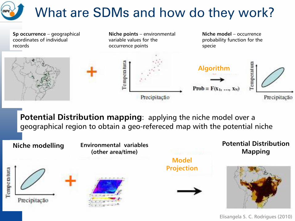
1. Formulation
Equilibrium
Important for general scale model
OK for persistent spp
Advantage: less physiology and behavior knowledge
Disadvantage: human influence, disturbs and successionalprocess are not included (individual behaviour, dispersion, migration, plasticity, adapatation, etc)
Static Models - consider equilibrium or pseudo-
equilibrium
Non-equilibrium: more realistic, BUT model should be dynamic and stochastic
Alternative – Dynamic simulation modelling Difficulty: knowledge about sp and environment relation, datasets
Modelling for what?What is the scientific question???

2. Data Preparation
SDMs – Species distribution models are empirical models relating field
observations to environmental predictor variables, based on
statistically or theoretically derived response surfaces.
Species occurrence data:
Presence, presence-absence, abundance; from field sampling or opportunistic - collections
Environmental predictors – direct or indirect effects
Limitation Factors (regulators): controlling eco-physiology (temp, H2O, soil)
Disturbances: disturbances (natural or anthropogenic) in the environment
Resources : any assimilable component (energy, nutrients, H2O)
Different spatial patterns according to the scale, hierarchically:

2. Data Preparation
Sampling and Data
Spatial Scale
Explicative variable (physiology) for preditive modelling
Sampling Desingn – GRADIENT Gradsect – (Gradient-Oriented Transect (Gradsect) Sampling)
Random-Stratified – random/sistematic sampling in homogeneus enviroment
Gradsect – for sp richness betterthan just sistematic or random
Data collected based on observation=> should samplie fixed sub-set fixo/ environmental estratum
Auto-correlation analysis to identifymimunum distance between samples

Specie occurence
Point Data
Latitude and longitude (cartography)
Spp identification (taxonomy)
Collection / project specialist inventories
Restrict area (usually small)
Sampling design – not planned for modelling
Geographical position can be imprecise
Data Availability– politics ("my data")
Interesting initiative -Biota-FAPESP and MCT
Data from Biological Collections and Herbarium

Specie occurence
Data from Scientific Herbaria
Classification System
Family, gender and specie
Appropriate storage
Suitable environmental conditions
Maria Cândida H. Mamede - IBt
Excicata
Herborization
Sp distribution – time and space
Flora from conserved disturbed areas
Taxonomic and phylogenetic studies
Precise sp identification (curator)
Associated collections
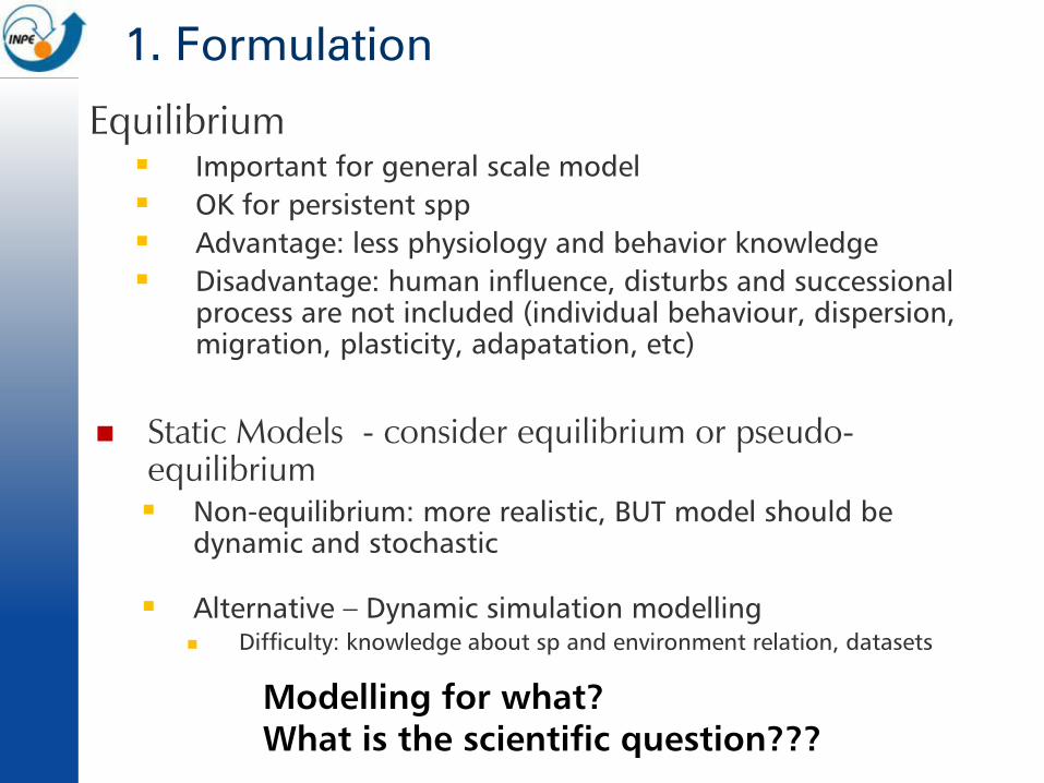
Specie occurence
Lable – informations – Geo-reference
Type
Maria Cândida H. Mamede - IBt

Specie occurence
Lable – informations – Geo-reference
Type
Maria Cândida H. Mamede - IBt

Specie occurence
Lable – informations – Geo-reference
Maria Cândida H. Mamede - IBt

Specie occurence
Database –
Data Cleaning
Taxonomic
Collections
Geographic UTM
GPS
DMS, ....
precision

http://splink.cria.org.br/tools?criaLANG=pt
Data &Tools

2. Data Preparation
SDMs – Species distribution models are empirical models relating field
observations to environmental predictor variables, based on
statistically or theoretically derived response surfaces.
Species occurrence data:
Presence, presence-absence, abundance; from field sampling or opportunistic - collections
Environmental predictors – direct or indirect effects
Limitation Factors (regulators): controlling eco-physiology (temp, H2O, soil)
Disturbances: disturbances (natural or anthropogenic) in the environment
Resources : any assimilable component (energy, nutrients, H2O)
Different spatial patterns according to the scale, hierarchically:

Gradual Distribution – large extend, corse resolution climatic regulators
Disperse Distribution – small area and fine resolution – controled by cluster resource distribution
(micro-topographic variation or habitat fragmentation)
SDM – limiting factors x sccale
–

Environmental Information
Field work, systematic mapping, remote sensing and GIS model resultant
DEM – important because of correlation with other variables. Precision. However low Predictive power
Topographic gradient can be useful to verify the correspondence between digital attributes and field data
TASK: select the adequate dataset to parameterize the model.
??? How selecting the predictive variables???
Based on the specialist knowledge of the group: minimum environmental requirements
Statistical procedures to select the predictive variables
stepwise for LS, GLMs and CCA
Jackknife, etc.
Data Preparation

Environmental variables
Usually selected – regional scales (!)
Climatic
Topographic
Soil
RS...
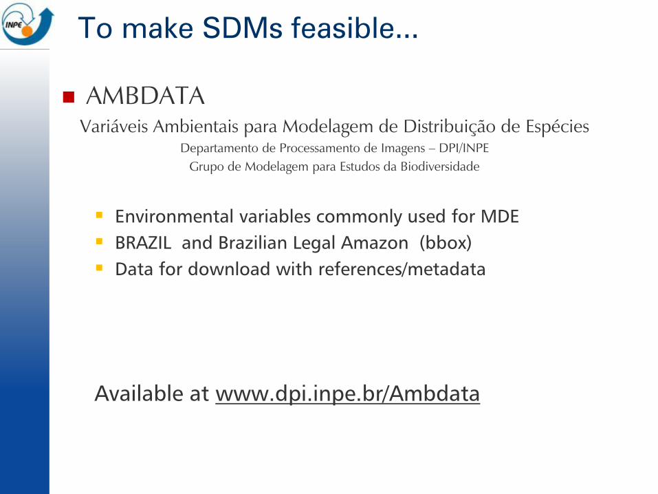
To make SDMs feasible...
AMBDATA
Variáveis Ambientais para Modelagem de Distribuição de Espécies
Departamento de Processamento de Imagens – DPI/INPE
Grupo de Modelagem para Estudos da Biodiversidade
Environmental variables commonly used for MDE
BRAZIL and Brazilian Legal Amazon (bbox)
Data for download with references/metadata
Available at www.dpi.inpe.br/Ambdata

To make SDMs feasible...
AMBDATA
Variáveis Ambientais para Modelagem de Distribuição de Espécies
Departamento de Processamento de Imagens – DPI/INPE
Grupo de Modelagem para Estudos da Biodiversidade
Variáveis ambientais normalmente usadas para MDE
Recorte BRASIL e Amazônia Legal
Dados para download com referências/metadados
Disponível em www.dpi.inpe.br/Ambdata

Statistical Model Formulation
Select an adequate algorithm to predict a certain responsevariable and estimate the model coefficients
Statistical models – most are specific to the probability distribution. Test: response variable statistical distribution
Generalized Regression
Relate a response variable to a single (simple) or a combination of (multiple) environmental variables (predictors)
Predictors - environmental var or derivate orthogonal components (avoid multi-collinearity) from multivariate analysis (PCs).
Classical regression (LR) - response variable has normal distributionand variance that does not change with the average (homoscedasticity)
3. Model Fitness

Generalized Regressions
GLMs – more flexible – response var. with other distributions and non-constant variance function
Linear Transformation
Predictions with values in a defined interval
Distributions: Gaussian, Poisson, Binomial or Gamma, and identity functions logarithmic, logistic e inverse
GAMs – Alternative regression: non-parametric functions to smooth the preditor Moving-averages – regression weighted by local or density functions weighted locally
Generalized Aditive Models – smoothes each predictor and calculates addictively the response variable; Multidimensional
Regression models can incorporate
ecological processes as dispersion or connectivity
Model Fitness

Classification Techniques
Classification trees (qualitative) and regression (quantitative) based on rules, or maximum likelihood.
It attributes a class for the response variable (binomial or multinomial) for every environmental predictors combination (nominal or continuous).
Model Fitness
Built from simple rules inter-relations from previous knowledge – literature, lab, observation, etc.

Environmental/climatic envelops – actual distribution x climatic
variables comparison envelop (hypercube) that describes the
environmental influence over specie variation
Climate Change scenarios simulation
Model Fitness
Elith & Leathwick, 2009

Environmental envelops
BIOCLIM – minimum retangular envelop in a multi-dimentional climatic space
HABITAT – more restrict space: convex hull envelops.
Model Fitness
DOMAIN – based on similarity metrics point-by-point (multivariate distance measures)
Environmental Distance (OM):
environmental dissimilarity distance;
Euclidian, Mahalanobis,Gower, etc.

Ordination techniques – spp or communities
Canonic Correspondence Analysis
Gradient direct analysis, principal ordination are linear combination of environmental data
Suppose Gaussian distribution for spp; lower and upper occurrence threshold and optimum along the gradient.
Very robust method. Adequate when absence data is abundant
Model Fitness

Bayesian approach
Combine a priori probability of a sp (community) observation with the probabilities related to every environmental predictor
Model Fitness
Conditional probability can be the rative frequency of a sp in a discrete class of a nominal preditor
P a priori can be based on literature
For vegetation mapping: P a posteriori is estimate for every vegetation unity
the unity with hishest P is associated to every candidate location

Neural Networks
Promissing tool : a few references for predicting sp space distribution based on biophysical variables
More powerefunn than miultivariate regression to model non-linear relations
Problem – non-parametric process of classification (“black art”)
Other approaches
ENFA – Ecological Niche-factor analysis –difers from CCA by considering one sp each time. Only presence data (animals).
MONOMAX –fits a monotonic max likelihood function iteractively
Discriminat function analysis
GIS Models – environmental overlay, variation metrics, similarity and rules to combine probabilites
Model Fitness

GARP
3
11
10
13
4
10
6
7
Fitness
11000000000000000001
10111010111000100101
10101000101001110110
11001110101011101101
00001000101000000100
11001010101010100101
00011000101010000010
11001000101000100100
População inicial
8
7
6
5
4
3
2
1
Ind.
3
11
10
13
4
10
6
7
Fitness
11000000000000000001
10111010111000100101
10101000101001110110
11001110101011101101
00001000101000000100
11001010101010100101
00011000101010000010
11001000101000100100
População inicial
8
7
6
5
4
3
2
1
Ind.
11001010101010100101
11001110101011101101
10101000101001110110
11001110101011101101
11001000101000100100
10111010111000100101
10101000101001110110
11001010101010100101
Cromossomos pais
3
5
6
5
1
7
6
3
Indivíduo
11001010101010100101
11001110101011101101
10101000101011101101
11001110101001110110
11001010111000100101
10111000101000100100
10101000101001100101
11001010101010110110
Cromossomos filhos
27
81
37
50
Sorteio
11001010101010100101
11001110101011101101
10101000101001110110
11001110101011101101
11001000101000100100
10111010111000100101
10101000101001110110
11001010101010100101
Cromossomos pais
3
5
6
5
1
7
6
3
Indivíduo
11001010101010100101
11001110101011101101
10101000101011101101
11001110101001110110
11001010111000100101
10111000101000100100
10101000101001100101
11001010101010110110
Cromossomos filhos
27
81
37
50
Sorteio
11001010101010100101
11001110101011101101
10101000101011101101
11001110101001110110
11001010111000100101
10111000101000100100
10101000101001100101
11001010101010110110
Cromossomos filhos
11001110101010100101
11001110101011101101
10101000101011101111
11001110101001110110
11001100101000100100
11111010111000100101
10101000101001110110
11101010101010000101
Cromossomos (mutação)
8
7
6
5
4
3
2
1
Indivíduo
11001010101010100101
11001110101011101101
10101000101011101101
11001110101001110110
11001010111000100101
10111000101000100100
10101000101001100101
11001010101010110110
Cromossomos filhos
11001110101010100101
11001110101011101101
10101000101011101111
11001110101001110110
11001100101000100100
11111010111000100101
10101000101001110110
11101010101010000101
Cromossomos (mutação)
8
7
6
5
4
3
2
1
Indivíduo
3
11
10
13
4
10
6
7
Fitness
11000000000000000001
10111010111000100101
10101000101001110110
11001110101011101101
00001000101000000100
11001010101010100101
00011000101010000010
11001000101000100100
População inicial
11001110101010100101
11001110101011101101
10101000101011101111
11001110101001110110
11001100101000100100
11111010111000100101
10101000101001110110
11101010101010000101
População 1a geração
8
7
6
5
4
3
2
1
Ind.
11
13
12
12
8
12
10
10
Fitness
3
11
10
13
4
10
6
7
Fitness
11000000000000000001
10111010111000100101
10101000101001110110
11001110101011101101
00001000101000000100
11001010101010100101
00011000101010000010
11001000101000100100
População inicial
11001110101010100101
11001110101011101101
10101000101011101111
11001110101001110110
11001100101000100100
11111010111000100101
10101000101001110110
11101010101010000101
População 1a geração
8
7
6
5
4
3
2
1
Ind.
11
13
12
12
8
12
10
10
Fitness
Aldair Santa Catarina (2006)
GARP - Genetic Algorithm for Rule-set Production
Genetic Algorithm to predict potential specie distribution from
environmental and biological data;
Automatic and um-supervised method;
Robust: tests several solutions and models (rules);
Maximize the significance and accuracy of prediction rules.

Maxent Potential probability distribution for the entire area
Distr Prob ?
Elisangela S. C. Rodrigues (2010)
Sp occurrence points
Environmental variables
Potential sp distribution estimate
Algorithm

Maxent
Data (no meaning ) = 25 - can be stored in the computer
Information (meaning associated) temperature = 25
(information can be represented by data)
Mean February max temperature = 25
二月份的平均最高氣溫 = 25
(this data represetation does not bring us any information)
Knowledge without knowing what is MEAN, the information does not
make any sense! (it depends on personal experience)
Entropy is a measure of disorder or predictability of a system. It
is a measure of uncertainty of an event
Unexpected observations have more information than expected observations !
Elisangela S. C. Rodrigues (2010)

Maxent
ENTROPY: is a measure of uncertainty of information
about the occurrence of an event
But if I have no previous idea, and an event occurs,
the entropy is greater because it brings me more information
It is s related to the probability of an event: the higher the probability
of an event, the lower the entropy.
If P is high the result is expected No information associated to the event.
If P is low It will be a asurprise! the event will bring information!
Maximum entropy: P is uniform.
If the dice has two sides #2, the entropy will be smaller because P(#2) will be
higher.
Uncertainty → surprise → information (or the entropy for an event, uncertainty)
Elisangela S. C. Rodrigues (2010)

Maxent
Entropy: uncertainty in an event, related to amount of information that
is transmitted when it occurs (“metric”)
Maximum entropy principle: from a set of possible probability
distribution, it must choose the Pdistr with present maximum entropy
i.e., that is most spread out, or closest to uniform, subject to a set of
constraints.
For that sp occurrence data and environmental layers a set of possible probability distribution
????
Choose/find the Pdist that provides more possible information – or the maximum entropy !
Probability Distribution
Elisangela S. C. Rodrigues (2010)

Maxent
Constraints=> represent the evidence, i.e. known facts about
input dataset. In our case: the environmental layers = features
X => geographic region
x1, x2,...,xn => observed/registered points
f1, f2,...,fn => features (layer values or a function of them )
Task: Having set points and layers, find the probability
distribution for this dataset:
Restrictons:
Features , evidences
(criteria about the layer values)
Probabilities Sum has to be = 1.
xn
x1
x2
x3
x4
Several possibleprobability distribuition
Elisangela S. C. Rodrigues (2010)

Maxent Maxent : estimate a target probability distribution by finding the probability distribution of
maximum entropy (i.e., that is most spread out, or closest to uniform), subject to a set
of constraints that represent our incomplete information about the target distribution.
There are several probability distribution that satisyes all the restrictions!!
(Then, the model is consistent and among then, it has to choose the one with contains maximum entropy!)
Find the weight for every features in a way that the result is the Max entropy
x1
x2
x3
x4
xn
The model express the adequacy of each cell as a function from environmental variables.
High maxent values for a cell indicates that it contains favorable condition for that specie! Prediction of favorable conditions!!!
From the model, projects to the geographical area, using environmental variables data set
http://www.cs.princeton.edu/~schapire/maxent/
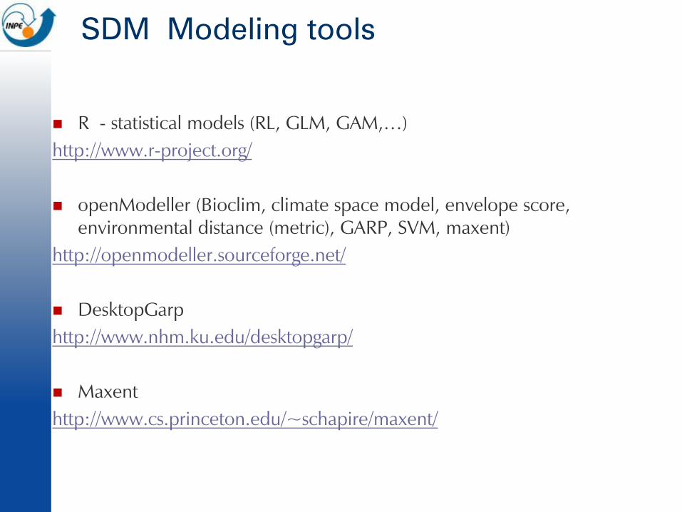
SDM Modeling tools
R - statistical models (RL, GLM, GAM,…)
http://www.r-project.org/
openModeller (Bioclim, climate space model, envelope score,
environmental distance (metric), GARP, SVM, maxent)
http://openmodeller.sourceforge.net/
DesktopGarp
http://www.nhm.ku.edu/desktopgarp/
Maxent
http://www.cs.princeton.edu/~schapire/maxent/

5. Predictions/ Model Results
Predict the potential sp distribution
Potential distribution maps OR cartographic representation of: Occurrence Probability ( GLMs logistics)
Likely Abundance (GLM ordinal)
Predicted Occurrence – non-probabilistic metric (CCA)
Likely Entity (from hierarchical analysis)
Occurrence Probability

6. Model evaluation
Validation –measure the adequacy between the predictcted model and
field observation (~accuracy for RS)
BUT Validation = formulation of the theory model
EVALUATION is better : not to verify if T or F, but for hypothesis testing and biological patterns prediction
Evaluation – as a measure of adequacy , dependent of the project
objectives and the application domain of the modeling
Usually :
Two independent datasets: training (to calibrate) and testing (evaluation)
Confusion matrix
Jack-knife, Cross Validation (CV) and/or bootstrap

6. Model evaluation Evaluation based on independent dataset
To calibrate and evaluate
split-sample – large dataset (Inadequate for small datasets)
Do not mix sampling and observational datasets
Confusion Matrix
Commission error are not errors from the model
Omission errors are serious!
Minimum predicted area:
predict smallest possible area of
sp potential occurrence
+ -
+ a b
- c dPredicted
Real
Omission Errors
Commission Errors
OmissionCommission
Real Geographical DistributionPredicted Geographical
Distribution
Iwashita (2007)

6. Model evaluation
JackKnife – Calculates confident intervals
Computed taking one observation off each time
Cross-validation – verifies the hypothesis if the result can be replicated
or it was just random
Part of dataset to calibrate the model and the other to test the error
Simple , double or Multi – repeats the pair several any times, selecting sub-samples
Bootstrap – addresses the deviation of the estimate performing
multiple re-sampling with replacement within the calibration dataset.
Obtaining an estimate without deviations.
Bias - difference between parameter estimate and the actual population value.
If the difference between the value obtained and corrected for deviation is very high, the adequacy of the model should be questioned

Model evaluation
Receiver operator characteristic (ROC-plot)
sensibility x especificity plot
Sensitivity is the probability
of a pixel x be correctly
classified as occurrence
Specificity is the probability of a
pixel be correctly
classified as absence
The closer to 1 is the area under
the curve - AUC, the better is
the model !
(BUT take care about the predicted area)

Research Perspectives
Environemtal Layers limitation
Accuracy and resolution from env data Remote sensing as additional data source. Precise
information about moisture, soil wetness, vegetation indices, land use class, etc.
Biotic Interactions Limitations
Competition – challenging.
Integrated systems of simultaneous regressions, GLMs?
Modeling system has to be close to equilibrium
From spp community modeling

Research Perspectives
Cause-effect Limitations
From Static models to space-temporal models??
Integration between eco-physiologist and succession dynamic modelers !
Historical Factors
Include biogeographical and evolutive factor into static SDMs. Place history
Sp absence in adequate environment – past geological or climatic events; physical barriers…
Organism history
Try to integrate evolution studies (phylogeny), population genetics, spp genetic integrity
Sampling design
Re-sampling strategies for modeling purposes, including environmental gradient

Research Perspectives
Space explicitly uncertainties evaluation
Include the uncertainties in the geographical space Important for model credibility and applicability;
Mapping of the uncertainties
Special auto-correlation
Auto-correlation and spatial variance of occurrence and environmental data
Include dispersion patterns in the modelling
Cellular automata
deal with neighborhood relations (spatial correlation) and dynamic
environments
Cells, their and transitions states –to model sp distribution of plants in climate change, simulation of migration of plants along corridors in segmented landscapes

SDMs – Remark
1. Formulation
2. Data Preparation
3. Model Fitness
4. Evaluation
5. Spatial predictions
6. Model usefullness
IMPORTANT: keep in mind the limitation and
assumptions in every step during the modelling
process

Normalized Difference Vegetation Index (NDVI) improving species distribution models: an example with the neotropical genus Coccocypselum (Rubiaceae)
Silvana Amaral
Cristina Bestetti Costa
Camilo Daleles Rennó
Divisão de Processamento de Imagens – DPI /INPE
XII Simpósio Brasileiro de Sensoriamento Remoto Florianópolis, April/2007

Context
The availability of observational data of species, and the scope
and resolution of spatially explicit environmental data, are
increasing,
Capabilities of the computational and analytical tools
Remote sensing data can contribute to the modeling process by improving the environmental data set and the niche characterization.
AVHRR/NOAA imagery, in combination with other variables, proved to have sufficient resolution to model the range of bird species.
METEOSAT temporal series was tested to improve climate data for wild life distribution models
Osborne et al, 2001

Context
Multi-temporal Normalized Difference Vegetation Index (NDVI) can be
used to model trends in species richness
The use of a vegetation index contributes providing information about
the canopy closure,
the phenological status
the water content variation within the different physiognomies.
We hypothesize that species distribution models that uses vegetation
index (NDVI) as an additional environmental variable would improve
the representation of a species spatial distribution.

Objective
This work analyses the contribution of
remote sensing data, specifically the NDVI,
for species distribution models, based on the
taxonomic revision of the neotropical genus
Coccocypselum P. Br.

The genus Coccocypselum
C. lanceolatum C. lanceolatum
C. hasslerianum C. erythrocephalum
Photo: C.B. Costa

The genus Coccocypselum
Genus Coccocypselum Rubiaceae family:
One of the most important families in the tropics.
Prostrate and creeping herbs with a spongy blue berries fruits.
18 species - small herbaceous genus, widely distributed in the Neotropics, south Mexico to northern Argentina
15 species occur in Brazil, 5 species selected.
Assumption: the observed species pattern is in a relative equilibrium with the environment

5:2:18
14:10:18
3:0:18
5:0:18
5:2:18
14:10:18
3:0:18
5:0:18
Geographic range and biodiversity
Source: Costa 2005
Coccocypsellum
Species
Distribution
C. anomalum Brazil – Atlantic coast
C. aureum Neotropics
C. bahiensis Brazil – Atlantic coast
C. capitatum Brazil – Atlantic coast
C. condalia Neotropics
C. cordifolium Neotropics
C. erythrocephamlum Brazil – Atlantic coast
C. geophiloides Equator, Colombia, Brazil, Bolívia
C. glabrifolium Brazil – Atlantic coast
C. guianense Central America, north of AS
C. hasslerianum Brazil, Bolivia, Paraguay,
Argentina
C. hirsutum Colombia, Venezuela, Guiana,
Peru, Brazil e Bolivia
C. hispidulum Central America, Colombia,
Venezuela, Trinidad, Peru
C. lanceolatum Neotropics
C. lymansmithii Brazil – Atlantic coast
C. pedunculare BA, MG
C. pulchellum PR, RS, SC
C. repens Central America and Antilles

Data Sources
Presence data:
taxonomic revision of Coccocypselum(Costa 2005)
Information associated with specimen vouchers in natural history museums.
Pseudo-absent data criteria:
Visited sites - species not recorded;
Visited sites, but other excluding species collected.
Not visited sites, but floristic studies did not record the species.
Sites that did not contain Coccocypselum species and the habitat is unsuitable.
Evaluation training set: 20% of the records
Training points Evaluation points Studied species
Presence Presence Absence
C. capitatum (Graham) C.B. Costa & Mamede 65 15 15
C. cordifolium Nees & Mart. 72 16 16
C. erythrocephalum Cham. & Schltdl. 33 8 8
C. lymansmithii Standl. 22 5 5
C. pulchellum Cham. 52 12 12

Data Sources / Tools
TerraView: TerraLib–OM Plugin
Species occurrences
Environmental variables
Results of species distribution
modeling

Environmental Variables
Selection based on specialist knowledge
general distribution of Coccocypselum genus is related to the conditions of humidity and altitudinal gradients
Nature Variables Resolution
(Degree) Source Date
Maximum temperature
Minimum temperature
Average temperature
Precipitation
Clima
Bioclimatic variables
0.25
Weather stations
WordClim Project
Average monthly climate data from 1950-2000 series
Elevation
Slope Relieve
Aspect
0.0089
SRTM
NASA
2000 imagery
Maximum NDVI
Minimum NDVI
Average NDVI
Vegetation RS
Standard deviation NDVI
1.0
AVHRR-17
NASA/CPTEC
Fortnightly mosaic 2005

Environmental Variables
AVHRR/NOAA17 -
NDVI
Derived measure of photosynthetic activity
Mosaic fortnightly series for 2005
Mosaic Images –cloud detection procedure – nodata values pixels
Images of NDVI Minimum, Maximum, Average and Standard Deviation

3
11
10
13
4
10
6
7
Fitness
11000000000000000001
10111010111000100101
10101000101001110110
11001110101011101101
00001000101000000100
11001010101010100101
00011000101010000010
11001000101000100100
População inicial
8
7
6
5
4
3
2
1
Ind.
3
11
10
13
4
10
6
7
Fitness
11000000000000000001
10111010111000100101
10101000101001110110
11001110101011101101
00001000101000000100
11001010101010100101
00011000101010000010
11001000101000100100
População inicial
8
7
6
5
4
3
2
1
Ind.
11001010101010100101
11001110101011101101
10101000101001110110
11001110101011101101
11001000101000100100
10111010111000100101
10101000101001110110
11001010101010100101
Cromossomos pais
3
5
6
5
1
7
6
3
Indivíduo
11001010101010100101
11001110101011101101
10101000101011101101
11001110101001110110
11001010111000100101
10111000101000100100
10101000101001100101
11001010101010110110
Cromossomos filhos
27
81
37
50
Sorteio
11001010101010100101
11001110101011101101
10101000101001110110
11001110101011101101
11001000101000100100
10111010111000100101
10101000101001110110
11001010101010100101
Cromossomos pais
3
5
6
5
1
7
6
3
Indivíduo
11001010101010100101
11001110101011101101
10101000101011101101
11001110101001110110
11001010111000100101
10111000101000100100
10101000101001100101
11001010101010110110
Cromossomos filhos
27
81
37
50
Sorteio
11001010101010100101
11001110101011101101
10101000101011101101
11001110101001110110
11001010111000100101
10111000101000100100
10101000101001100101
11001010101010110110
Cromossomos filhos
11001110101010100101
11001110101011101101
10101000101011101111
11001110101001110110
11001100101000100100
11111010111000100101
10101000101001110110
11101010101010000101
Cromossomos (mutação)
8
7
6
5
4
3
2
1
Indivíduo
3
11
10
13
4
10
6
7
Fitness
11000000000000000001
10111010111000100101
10101000101001110110
11001110101011101101
00001000101000000100
11001010101010100101
00011000101010000010
11001000101000100100
População inicial
11001110101010100101
11001110101011101101
10101000101011101111
11001110101001110110
11001100101000100100
11111010111000100101
10101000101001110110
11101010101010000101
População 1a geração
8
7
6
5
4
3
2
1
Ind.
11
13
12
12
8
12
10
10
Fitness
3
11
10
13
4
10
6
7
Fitness
11000000000000000001
10111010111000100101
10101000101001110110
11001110101011101101
00001000101000000100
11001010101010100101
00011000101010000010
11001000101000100100
População inicial
11001110101010100101
11001110101011101101
10101000101011101111
11001110101001110110
11001100101000100100
11111010111000100101
10101000101001110110
11101010101010000101
População 1a geração
8
7
6
5
4
3
2
1
Ind.
11
13
12
12
8
12
10
10
Fitness
Species Distribution Modeling
To evaluate the importance of NDVI:
climatologic and topographic variables
climatologic and topographic variables +NDVI
Genetic Algorithm for Rule-Set Production (GARP) Best
sub-set, in the OpenModeller (OM).
Gerar uma população
Estimar a população
Parar
Seleção
Cruzamento
Mutação
Estimação da nova população
Não
Sim
Fim da busca?
Source: Santa Catarina, 2006

Species Distribution Modeling
GARP Best-subset
random approach, 10 models per species.
result is a summary with the potential distribution (%)
Statistical Test
Comparison: models with and without NDVI data
Confusion Matrix: presence and absence evaluation points
Are the models different from what would be expected from a random classification?? Kappa statistic
Different number of evaluation points=> non-parametric statistic to compare samples: the Mann-Whitney test (U)
Evaluation of sample size effect
Compare models – smaller U statistic, better models.

Coccocypselum Distributions
Coccocypselum species - wet forest, along rivers and wet places.
The NDVI data incorporated to models can predict a relation between the
species in open or more forested physiognomy.
C. cordifolium modeled with climatic and topography data. C. cordifolium modeled with climatic, topography and NDVI data.

Coccocypselum Distributions
Predicted distribution map with NDVI reveals a more restricted pattern for
all species of Coccocypselum studied.
C. capitatum and C. cordifolium present a wider distributional pattern. The
others species have a more restricted range and the models seem to be more
accurate.
C. erythrocephalum - climatic and topography data. C. erythrocephalum - climatic, topography and NDVI data.
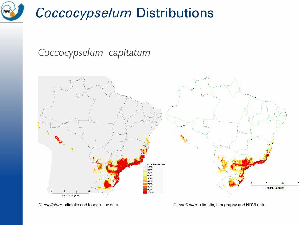
Coccocypselum Distributions
Coccocypselum capitatum
C. capitatum - climatic and topography data. C. capitatum - climatic, topography and NDVI data.

Coccocypselum Distributions
Coccocypselum lymansmithii
C. lymansmithii - climatic and topography data. C. lymansmithii - climatic, topography and NDVI data.

Coccocypselum Distributions
Coccocypselum pulchellum
C. pulchellum - climatic and topography data. C. pulchellum - climatic, topography and NDVI data.

Coccocypselum Distributions
The usefulness of the environmental niche modeling when applied
to biogeographical and conservation approaches has been
contested (Araújo and Guisan 2006).
The species distribution models shows a result consistent to the
distributional observation found in the taxonomic study of the
genus Coccocypselum (Costa 2005).
As expected, the SDM showed a wider distributional pattern.
SDM can be improved by restricting the predicted ranges using
expert drawn range maps and biogeographical regions information.

Statistical Analysis
Kappa analysis
values higher than 0.5 => good fit between the evaluation points and the modeled species distribution.
The models were better than random.
Models with NDVI were NOT superior to those fitted with climatic and topographical predictors only.
Mann-Whitney test
Only C. pulchellum, C. capitatum and C. cordifolium models differentiated statistically between the presence and absence occurrence data.
C. lymansmithii and C. erythrocephalum the distribution model was not conclusive.
Limited distribution of theses species and the low number of samples points (<10).
Kappa Mann-Whitney (U Statistic)
Specie
no NDVI NDVI no NDVI NDVI
Critical value
(α =5%) N
C. lymansmithii 0.8 0.8 7.5 7.5 2 5
C. erythrocephalum 0.5 0.5 21.5 22.5 12 8
C. pulchellum 0.83 0.83 16* 15* 37 12
C. capitatum 0.6 0.53 55* 48.5* 64 15
C. cordifolium 0.75 0.56 46.5* 36* 75 16
* Significative at 5%

Contribution
The species distribution models generate by GARP indicates a potential
presence of the species studied closely related to the known distribution of
the species studied.
The models for wide distribution species (C. capitatum and C. cordifolium),
were more consistent to the real distribution then the restrict ones
(C. lymansmithii, C. erythrocephalum and C. pulchellum).
It presents a very robust statistical analysis of the models, since absent data
were generated exclusively for this purpose. Approach is not frequent in the
species distribution modeling analysis by the difficulty of having absence data.

Contribution
Comparing the species distribution models generated including NDVI data,
they presented better results than the distribution models generated without
NDVI data.
Despite the values were very similar, this results suggested an improvement
when using NDVI as environmental variables in the modeling process.
This study illustrated the potential of incorporating NDVI data into large-
scale models of plant species distribution.
The same approach should be applied over other species with higher sample
size for more accurate analysis.

SEM
coord.
64,72%
COM coord.
válidos
27,69%
(2637
ou
77,79%)
COM
coord.
35,28%
(3360)
erros
7,59%
(723 ou
21,33%)
Pam species occurrence database for SDMs
São Paulo – 763 reg.
Amazonas –
427 reg.
Acre – 298 reg.Bahia – 298 reg.
Mato Grosso – 129 reg.
Goiás – 106 reg.
Pará – 99 reg.
Maranhão – 94 reg.
São Paulo – 763 reg.
Amazonas –
427 reg.
Acre – 298 reg.Bahia – 298 reg.
Mato Grosso – 129 reg.
Goiás – 106 reg.
Pará – 99 reg.
Maranhão – 94 reg.• TOTAL 9524 records;• 3360 with geographic coordinates• 2637 records after initial corrections (coordinates in the sea, replication, taxonomy )
• Richer genders : Bactris (38spp.), Geonoma (37), Syagrus(25), Attalea (22) and Astrocaryum (13).
Arasato et al., 2007

Arasato et al., 2007
Registros /spp
No Brasil
São Paulo – 763 reg.
Amazonas –
427 reg.
Acre – 298 reg.Bahia – 298 reg.
Mato Grosso – 129 reg.
Goiás – 106 reg.
Pará – 99 reg.
Maranhão – 94 reg.
São Paulo – 763 reg.
Amazonas –
427 reg.
Acre – 298 reg.Bahia – 298 reg.
Mato Grosso – 129 reg.
Goiás – 106 reg.
Pará – 99 reg.
Maranhão – 94 reg.
Pam species occurrence database for SDMs

Environmental variables
WORLDCLIM.ORG (10arc-min or +18,5km)
Climate: temperatures, minimum and maximum, and precipitation for January and July;
Bioclimatic: bio1, bio4, bio13
SRTM (Shuttle Radar Topography Mission)
Altitude, slope and aspect: ~ 1 km
HAND: 30 arc-sec ou +1km ; limiar de 100
Densidade de drenagem (Kernel): r.e. 10 km; raio de influência de 43000 km²
HAND: 30 arc-sec or +1 km; 100 limiar for drainage Density (Kernel): r.e. 10 km; radius of influence of 43000 km²
Algorithms
Maxent: http://www.cs.princeton.edu/~schapire/maxent
GARP best subset: http://openmodeller.sourceforge.net/
Drainage Density and SRTM - HAND do SRTM for Palm species distribution modelling
Arasato et al., 2009
Euterpe edulis Mart.

A
GARP
B
Maxent
A
no DDren
B
DDren
Resultados
GARP – very generalised
Distribution of Euterpe edulis Mart., proved really dependent
on the seasonality of temperature (bio4) and the availability of
water (prec and drainage density), this order, as indicated by
literature
Data from SRTM, drainage density, and HAND were not
sufficient to override other relieve variables
Drainage Density and SRTM - HAND do SRTM for Palm species distribution modelling

A
no HAND
B
HAND
A
GARP
B
Maxent
Results
The best model was the resulting from the
use of variable altitude, slope, aspect,
drainage density and hand to define the
limits of distribution of Euterpe Edulis
Drainage Density and SRTM - HAND do SRTM for Palm species distribution modelling

Remarks
SDM has many limitations...
A tool to understand the variables/processes that defines sp
distribution
Ex. Can be useful for conservation
Input Database precision & trustworthy sp occurrence data
Remote Sensing and geoinformation basic for modeling
Georeferecing
Environmental variables – precision and temporal cover

Our Biodiversity group...
Silvana Amaral
Dalton Valeriano
Cristina B. Costa
Luciana S. Arasato
Diana Valeriano
Camilo Rennó
Marco Antonio Ribeiro Jr.
Arimatéa de C. Ximenes

Study Group

Biodiversity
Based on environmental variability
Self Organizing Mapping (SOM) for ecoregions definition/mapping
Arimatea C. Ximenes
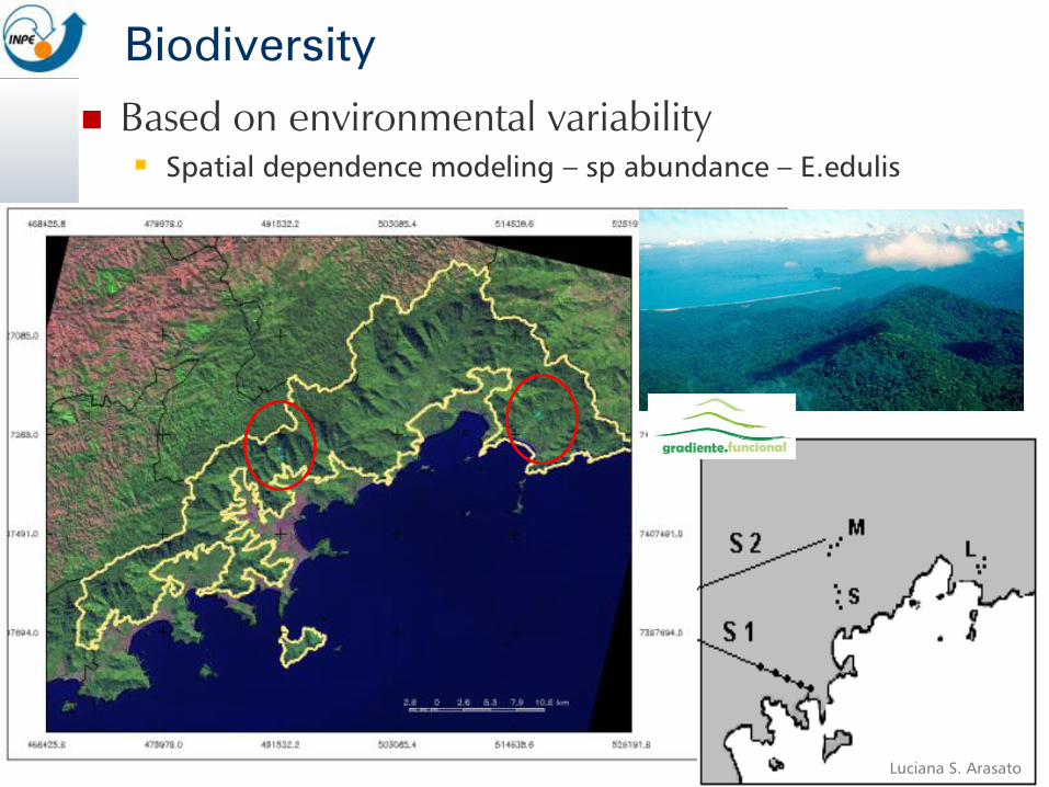
Biodiversity
Based on environmental variability
Spatial dependence modeling – sp abundance – E.edulis
DEM / Hand
Occurence data (palmeiras)
Luciana S. Arasato

Biodiversity
DEM / Hand
Spatial dependence modeling – Arecaceae
Luciana S. Arasato

HAND x Abundance + spatial correlation
Atlantic Rain Forest – Arecaceae (palm trees)
Biodiversity
Occurrence data
Pontos de altitude
Curvas de nível
Luciana S. Arasato

Based on Phylogenetic Richness
Amazon Forest – trees from RadamBrasil invetory
Biodiversity
Cristina B. Costa

Based on Phylogenetic Richness
Amazon Forest – trees from RadamBrasil invetory Conservation issues
Biodiversity
Cristina B. Costa

Based on life forms – BOX model
Contact Amazon Forest / Cerrado
FLORESTA AMAZÔNICA CERRADO
Arborescentes perenifólias Arborescentes de tronco suculento
Arbustos em roseta mesófilos (palmeiras anãs) Arbustos em roseta mesófilos (palmeiras anãs)
Arbustos em roseta xerófilos (bromélias terrestres) Arbustos em roseta xerófilos (bromélias terrestres)
Arbustos espinhentos caducifólios Arbustos espinhentos caducifólios
Arbustos latifoliados perenifólios tropicais Arbustos latifoliados perenifólios tropicais
Árvores baixas latifoliadas caducifólias Árvores anãs latifoliadas perenifólias tropicais
Árvores caducifólias mesófilas Árvores baixas latifoliadas caducifólias
Árvores caducifólias xerófilas Árvores caducifólias mesófilas
Árvores de floresta pluvial tropical Árvores palmiformes (palmeiras)
Árvores palmiformes (palmeiras) Árvores microfilas perenifólias tropicais
Árvores microfilas perenifólias tropicais Árvores pequenas de floresta montana
Árvores pequenas latifoliadas perenifólias tropicais Árvores pequenas latifoliadas perenifólias tropicais
Árvores perenifólias de região temperada quente Arvoretas palmiformes (palmeiras baixas)
Arvoretas palmiformes (palmeiras baixas) Epífitas de folha estreita
Epífitas de folha estreita Epífitas latifoliadas caducifólias
Ervas latifoliadas perenifólias tropicais Ervas latifoliadas caducifólias
Ervas latifoliadas suculentas Ervas latifoliadas perenifólias tropicais
Gramíneas altas (típicas) Ervas latifoliadas suculentas
Gramíneas altas (tipo cana) Gramíneas altas (típicas)
Gramíneas arborescentes Gramíneas altas (tipo cana)
Gramíneas pequenas (em tufo) Gramíneas arborescentes
Gramíneas pequenas (tipo gramado) Gramíneas pequenas (em tufo)
Hemiepífitas Gramíneas pequenas (em touceira espessa)
Lianas latifoliadas perenifólias tropicais Gramíneas pequenas (tipo gramado)
Palmeiras trepadeiras Lianas latifoliadas perenifólias tropicais
Pteridófitas perenifólias Trepadeiras latifoliadas caducifólias
Trepadeiras latifoliadas perenifólias
Biodiversity
André Jardim
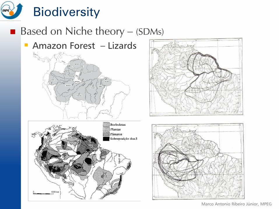
Based on Niche theory – (SDMs)
Amazon Forest – Lizards
Biodiversity
Marco Antonio Ribeiro Júnior, MPEG

Based on Niche theory – (SDMs)
Amazon Forest – Lizards
Biodiversity
Marco Antonio Ribeiro Júnior, MPEG

Based on Niche theory – (SDMs)
Amazon Forest – Lizards
Biodiversity
OG
RO
SW WSE
EGui
WGui
Similarity between
areas
Environmental
factors and
distribution patterns
PhylogenyScenarios
Hypothesis about evolution context for the biogeography scenarios associating:
Marco Antonio Ribeiro Júnior, MPEG

Based on Niche theory – (ARECACEAE SDM)
http://www.dpi.inpe.br/Ambdata/index.php (Rubiaceae, Croton, Poaceae,...)
Biodiversity

Based on Individual / community modelling
NE Brazilian coast - Mangrove forest -spp succession
Ombrophylous Mixed Forest in Southeast Brazil - Tree Species –TROLL (?)
Biodiversity
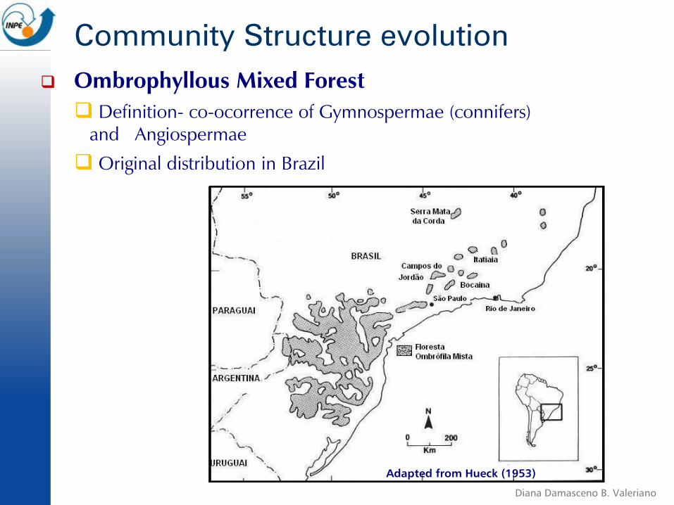
Ombrophyllous Mixed Forest
Definition- co-ocorrence of Gymnospermae (connifers)
and Angiospermae
Original distribution in Brazil
Adapted from Hueck (1953)
Community Structure evolution
Diana Damasceno B. Valeriano

Araucaria Forest BiogeographyPast (~200.000 km2) x Present (~2%)
Large emergent trees – defines the forest structure – long life span –recruitment failure in the absence of large disturbances
Diana Damasceno B. Valeriano

Biogeography
Mixed Araucaria Forests –
exclusive of Southern
Hemisphere
Two species in South
America:
• Araucaria araucana (Chile)
• Araucaria angustifolia (Brazil)
Life History & Structure
Monodominance of long-lived
pioneers
(Large emergent trees – defines the
forest structure – long life span –
recruitment failure in the absence of
large disturbances)
Araucaria Forest
Diana Damasceno B. Valeriano

Mixed Forests with Monodominance of Connifers:
1. Biogeographical Model of Forest Expansion (Klein 1960) – Connifers expansion in open areas – failure to recrute inside the forest
2. Gap Model – autogenic succession (Jarenkow & Batista 1987) – gap from a fallen connifer – allows regeneration
3. Temporal Plot Replacement Model (Lozenge) (Ogden & Stewart 1995) - intermittent recruitment dependent of severe disturbances
Dynamic Models for Mixed Forests
Diana Damasceno B. Valeriano

Study AreaCampos do Jordão State Park, SP
Diana Damasceno B. Valeriano

Forests and High Altitude Fields Mosaic(Campos do Jordão State Park - Ikonos Satellite Image – 2005)
Diana Damasceno B. Valeriano

Methods:
1. Permanent plot (0.5ha)
2. Two inventories – 20 years apart (1988 – 2008)
3. Biometric and floristic data of all trees with dbh ≥ 1.6cm
4. All trees had their position recorded (x,y coordinates- 0.1m precision) and received an identification tag
Main Goal: to evaluate the forest dynamics
1.Mature forest or under ongoing succession?
2.Which model better describes the forest dynamics?
Approachs:
1.Structural and Floristic dynamics
2.Dominant Population Dynamics
3.Horizontal Structural Dynamics (exploratory)
Forest Dynamic - 20 years apart
Diana Damasceno B. Valeriano

Height stratification
1988 (t1) - 2008 (t2)Dominant tree populations (cover value)(14 species - )
emergents
canopy
understory
Diana Damasceno B. Valeriano

Diameter stratification1988 (t1) - 2008 (t2)Dominant tree populations (14 species)
Emergents canopy understory(exclusive)
Diana Damasceno B. Valeriano

Tree Locations - Surface Density MapsKernel Spatial Interpolation
Understorey 2008
Understory1988 Dominant1988
Dominant 2008
N88_understory x N88_dominant
r = -0,73
N08_understory x N08_dominant
r = 0,06
Diana Damasceno B. Valeriano

Mortality and Recruitment Surface DensityMaps
Kernel Spatial Interpolation
Chablis areas
= 1988 mapped logs;
= 2008 mapped logs
(darker’s over lighter’s).
A. angustifolia and P. lambertii - dap ≥ 50cm (stars)
Diana Damasceno B. Valeriano
Modelling Forest Dynamics
The question:
What is the stage of Campos do Jordão Mixed Forest: Dynamic
equilibrium /mature forest? under ongoing succession?
GOAL
To predict the effect of forest dynamics on tree biomass,
structure and species composition
Use of spatially explicit forest models - TROLL???
Steps:
1. Group species into functional types
2. Discriminate height groups
3. Parameterization of growth, mortality, recruitment rates
4. Characterize tree population structure (dbh) and successionalpattern
Diana Damasceno B. Valeriano

Thank you!
No hard questions, please!!
(Take a look at our “Referatas” - www.dpi.inpe.br/referata)
“All models are wrongbut some are useful!”
(Box, 1979).
References
Guisan, A. ; Thuiller, W. 2005, Predicting species distribution: offering
more than simple habitat. Ecology Letters, 8:993-1009.
Guisan, A. ; Zimmermann. 2000, Predictive habitat distribution models
in ecology. Ecological Modelling, 135:147-186.
Ambdata (http://www.dpi.inpe.br/Ambdata/index.php)
Referatas (http://www.dpi.inpe.br/referata/)
IWASHITA, F. Sensibilidade de modelos de distribuição de espécies a erros de
posicionamento de dados de coleta. 2007. 103 p. (INPE-15174-TDI/1291). Dissertação
(Mestrado em Sensoriamento Remoto) - Instituto Nacional de Pesquisas Espaciais, São José
dos Campos, 2007. Disponível em: <http://urlib.net/sid.inpe.br/mtc-
m17@80/2007/06.13.12.04>. Acesso em: 06 abr. 2011.

References
XIMENES, A. C. ; AMARAL, S. ; VALERIANO, D. M. . O conceito de ecorregião e os métodos utilizados para o seu
mapeamento. Geografia (Rio Claro. Impresso), v. 35, p. 219-226, 2010.
FOOK, K. D. ; AMARAL, S. ; MONTEIRO, Antônio Miguel Vieira ; CAMARA, Gilberto ; XIMENES, A. C. ; ARASATO, L. S. .
Making species distribution models available on the web for reuse in biodiversity experiments: euterpe edulis species case
study. Sociedade & natureza (UFU. Online), v. 21, p. 39-49, 2009.7.
FOOK, K. D. ; AMARAL, S. ; Vieira Monteiro, Antônio Miguel ; CÂMARA, Gilberto ; Casanova, Marco Antônio ; Amaral,
Silvana . Geoweb Services for Sharing Modelling Results in Biodiversity Networks. Transactions in GIS, v. 13, p. 379-399,
2009.
XIMENES, A. C. ; AMARAL, S. . Mapeamento das Ecorregiões do Distrito Florestal Sustentável da BR-163 na Amazônia
Brasileira com uso de redes neurais. In: SIMPÓSIO BRASILEIRO DE SENSORIAMENTO REMOTO, 15. (SBSR), 2011,
Curitiba, PR. SIMPÓSIO BRASILEIRO DE SENSORIAMENTO REMOTO, 15. (SBSR). São José dos Campos : INPE, 2011. p.
3094-3102.
ARASATO, L. S. ; AMARAL, S. ; RENNÓ, C. D. . Detecting individual palm trees (Arecaceae family) in the Amazon
rainforest using high resolution image classification. In: SIMPÓSIO BRASILEIRO DE SENSORIAMENTO REMOTO, 15.
(SBSR), 2011, Curitiba, PR. SIMPÓSIO BRASILEIRO DE SENSORIAMENTO REMOTO. São José dos Campos : INPE, 2011.
p. 7628-7635.
ARASATO, L. S. ; AMARAL, S. ; XIMENES, A. C. . Densidade de drenagem e HAND (Height Above the Nearest Drainage)
do SRTM para modelagem de distribuição de espécie de palmeiras no Brasil. In: SIMPÓSIO BRASILEIRO DE
SENSORIAMENTO REMOTO, 14, 2009, Natal. SIMPÓSIO BRASILEIRO DE SENSORIAMENTO REMOTO, 14., 2009.
XIMENES, A. C. ; AMARAL, S. ; ARCOVERDE, G. F. B. ; MONTEIRO, Antônio Miguel Vieira . Redes neurais para a seleção
de variáveis ambientais no processo de modelagem de distribuição de espécies na região Norte do Brasil. In: XIV
SIMPÓSIO BRASILEIRO DE SENSORIAMENTO REMOTO, 2009, Natal. XIV SIMPÓSIO BRASILEIRO DE
SENSORIAMENTO REMOTO. São José dos Campos : INPE, 2009.
FOOK, K. D. ; AMARAL, S. ; MONTEIRO, Antônio Miguel Vieira ; CAMARA, Gilberto . Sharing executable models through
an Open Architecture based on Geospatial Web Services: a Case Study in Biodiversity Modelling. In: GEOINFO, 2008,
Rio de Janeiro. Geoinfo, 2008.

References AMARAL, S. ; COSTA, C. B. ; RENNÓ, C. D. . Normalized Difference Vegetation Index (NDVI) improving species
distribution models: an example with the neotropical genus Coccocypselum (Rubiaceae). In: XIII Simpósio Brasileiro de
Sensoriamento Remoto, 2007, Florianópolis, 2007.
XIMENES, A. C. ; RIBEIRO, J. R. ; AMARAL, S. . Mapas auto-organizáveis e parâmetros geofísicos para a caracterização da
heterogeneidade de paisagens. In: XIII Simpósio Brasileiro de Sensoriamento Remoto, 2007, Florianópolis, 2007.
IWASHITA, Fabio ; AMARAL, S. ; MONTEIRO, Antônio Miguel Vieira ; Friedel, M. J. . Evaluating the effects of positioning
errors on the accuracy of species distribution models using synthetic data. In: he 3rd USGS Modeling Conference, 2010,
Denver, Colorado, EUA. 3rd USGS Modeling Conference: Understanding and Predicting for a Changing World, 2010.
ARASATO, L. S. ; AMARAL, S. ; RENNÓ, C. D. ; FISH, S. T. V. . MODELAGEM DE DISTRIBUIÇÃO DE Euterpe edulis
MART. NO BRASIL: USO DE INFERÊNCIA FUZZY. In: XVIII Congresso da Sociedade Botânica de São Paulo, 2010, São
Paulo. XVIII Congresso da Sociedade Botânica de São Paulo, 2010.
ARASATO, L. S. ; AMARAL, S. ; COSTA, C. B. . Banco de dados de palmeiras para modelagem de distribuição de
espécies. In: Conferência Científica Internacional LBA/GEOMA/PPBio. Amazônia em Perspectiva: Ciência Integrada para
um Futuro Sustentável Manaus, LBA/GEOMA/PPBio, 2008, Manaus. Conferência Científica Internacional
LBA/GEOMA/PPBio., 2008
JARDIM, A. C. ; VINHAS, L. ; CAMARA, Gilberto ; AMARAL, S. . Implementação de uma base de dados ambientais
remota para modelagem de biodiversidade. In: Conferência Científica Internacional LBA/GEOMA/PPBio. Amazônia em
Perspectiva: Ciência Integrada para um Futuro Sustentável, 2008, manaus. Conferência Científica Internacional
LBA/GEOMA/PPBio, 2008.
JARDIM, A. V. F. ; AMARAL, S. ; COSTA, C. B. ; VALERIANO, D. M. . Impacto das mudanças climáticas na composição de
formas de vida de plantas na fronteira entre Amazônia e Cerrado: dados preliminares. In: Conferência Científica
Internacional LBA/GEOMA/PPBio. Amazônia em Perspectiva: Ciência Integrada para um Futuro Sustentável, 2008.
Conferência Científica Internacional LBA/GEOMA/PPBio.
XIMENES, A. C. ; AMARAL, S. ; MONTEIRO, Antônio Miguel Vieira . Mapas auto-organizáveis para identificação de
ecorregiões no interflúvio Madeira-Purus: uma abordagem da biogeografia ecológica. In: Conferência Científica
Internacional LBA/GEOMA/PPBio. Amazônia em Perspectiva: Ciência Integrada para um Futuro Sustentável, 2008,
manaus. Conferência Científica Internacional LBA/GEOMA/PPBio, 2008.