
U.S. Fish & Wildlife Service Mourning Dove, White-winged Dove
45
Mourning Dove, White-winged Dove, and Band-tailed Pigeon 2009 Population Status U.S. Fish & Wildlife Service
Transcript of U.S. Fish & Wildlife Service Mourning Dove, White-winged Dove

Mourning Dove, White-winged Dove, and Band-tailed Pigeon2009 Population Status
U.S. Fish & Wildlife Service

Mourning Dove, White-winged Dove, and Band-tailed Pigeon Population Status, 2009 Edited by: Todd A. Sanders U.S. Fish and Wildlife Service Division of Migratory Bird Management Population and Habitat Assessment Branch 11510 American Holly Drive Laurel, MD 20708-4002 June 2009 Cover photograph: White-winged dove by Roy Tomlinson Suggested citations: Sanders, T. A., editor. 2009. Mourning dove, white-winged dove, and band-tailed pigeon population
status, 2009. U.S. Fish and Wildlife Service, Laurel, Maryland, USA. Dolton, D. D., T. A. Sanders, and K. Parker. 2009. Mourning dove population status, 2009. Pages 1–22
in T. A. Sanders, editor. Mourning dove, white-winged dove, and band-tailed pigeon population status, 2009. U.S. Fish and Wildlife Service, Laurel, Maryland, USA.
Rabe, M. J. 2009. White-winged dove status in Arizona, 2009. Pages 25–32 in T. A. Sanders, editor.
Mourning dove, white-winged dove, and band-tailed pigeon population status, 2009. U.S. Fish and Wildlife Service, Laurel, Maryland, USA.
Sanders, T. A. 2009. Band-tailed pigeon population status, 2009. Pages 33–42 in T. A. Sanders, editor.
Mourning dove, white-winged dove, and band-tailed pigeon population status, 2009. U.S. Fish and Wildlife Service, Laurel, Maryland, USA.
All Division of Migratory Bird Management reports are available on our home page at: http://www.fws.gov/migratorybirds

MOURNING DOVE POPULATION STATUS, 2009 DAVID D. DOLTON, U.S. Fish and Wildlife Service, Division of Migratory Bird Management, PO Box 25486 DFC,
Denver, CO 80225-0486, USA TODD A. SANDERS, U.S. Fish and Wildlife Service, Division of Migratory Bird Management, 911 NE 11th Avenue,
Portland, OR 97232-4181, USA KERI PARKER, U.S. Fish and Wildlife Service, Division of Migratory Bird Management, Patuxent Wildlife Research
Center, 11510 American Holly Drive, Laurel, MD 20708-4002, USA Abstract: This report summarizes information on the abundance and harvest of mourning doves collected annually in the United States. The focus is on results from the Mourning Dove Call-count Survey, but also includes results from the Breeding Bird Survey and the Migratory Bird Harvest Information Program. According to the Call-count survey, the mean number of doves heard per route over the recent 2 years (2008–2009) increased significantly in the Central Management Unit, but did not change significantly in either the Eastern or Western Units. Over the most recent 10 years (2000–2009), there was no significant trend in doves heard for either the Eastern or Western Management Units while the Central Unit declined significantly. Over the 44-year period (1966–2009), there was no significant change in doves heard for the Eastern Unit while the Central and Western Units declined significantly. Based on the mean number of doves seen per route, however, there was no significant change for any of the three Management Units during the recent 10-year period. Over 44 years, there was no change in doves seen for the Eastern and Central Units while the Western Unit declined significantly. The mourning dove (Zenaida macroura) is one of the most abundant species in urban and rural areas of North America, and is familiar to millions of people. Authority and responsibility for management of this species in the United States is vested in the Secretary of the Interior. This responsibility is conferred by the Migratory Bird Treaty Act of 1918 which, as amended, implements migratory bird treaties between the United States and other countries. Mourning doves are included in the treaties with Great Britain (for Canada) and Mexico (U.S. Department of the Interior 1988). These treaties recognize sport hunting as a legitimate use of a renewable migratory bird resource. The annual harvest is estimated to be between 5 and 10% of the population (Otis et al. 2008a). Maintenance of mourning dove populations in a healthy, productive state is a primary management goal. Management activities include population assessment, harvest regulation, and habitat management. Each year, counts of mourning doves heard and seen are conducted by state, federal, tribal, and other biologists in the 48 conterminous states to monitor
mourning dove populations. The resulting information is used by wildlife administrators in setting annual hunting regulations. A history of dove hunting regulations is provided in Appendix A. DISTRIBUTION AND ABUNDANCE Mourning doves breed from southern Canada throughout the United States into Mexico, Bermuda, the Bahamas and Greater Antilles, and in scattered locations in Central America (Fig. 1). While mourning doves winter throughout much of the breeding range, the majority winter in the southern United States, Mexico, and south through Central America to western Panama (Aldrich 1993, Mirarchi and Baskett 1994). The mourning dove is one of the most widely distributed and abundant birds in North America (Peterjohn et al. 1994, Fig. 1). The fall population for the United States was recently estimated to be about 350 million (Otis et al. 2008b). The primary purpose of this report is to facilitate the
prompt distribution of timely information. Results are preliminary and may change with the inclusion of additional data.
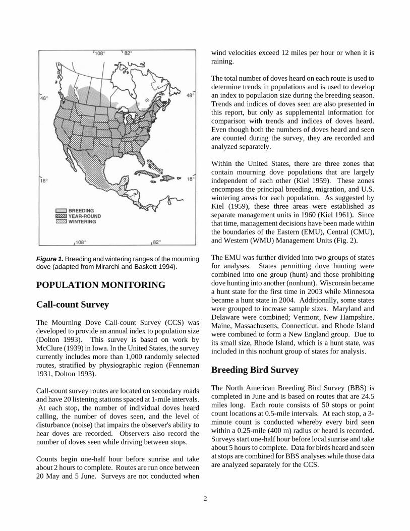
Figure 1. Breeding and wintering ranges of the mourning dove (adapted from Mirarchi and Baskett 1994). POPULATION MONITORING Call-count Survey The Mourning Dove Call-count Survey (CCS) was developed to provide an annual index to population size (Dolton 1993). This survey is based on work by McClure (1939) in Iowa. In the United States, the survey currently includes more than 1,000 randomly selected routes, stratified by physiographic region (Fenneman 1931, Dolton 1993). Call-count survey routes are located on secondary roads and have 20 listening stations spaced at 1-mile intervals. At each stop, the number of individual doves heard calling, the number of doves seen, and the level of disturbance (noise) that impairs the observer's ability to hear doves are recorded. Observers also record the number of doves seen while driving between stops. Counts begin one-half hour before sunrise and take about 2 hours to complete. Routes are run once between 20 May and 5 June. Surveys are not conducted when
wind velocities exceed 12 miles per hour or when it is raining. The total number of doves heard on each route is used to determine trends in populations and is used to develop an index to population size during the breeding season. Trends and indices of doves seen are also presented in this report, but only as supplemental information for comparison with trends and indices of doves heard. Even though both the numbers of doves heard and seen are counted during the survey, they are recorded and analyzed separately. Within the United States, there are three zones that contain mourning dove populations that are largely independent of each other (Kiel 1959). These zones encompass the principal breeding, migration, and U.S. wintering areas for each population. As suggested by Kiel (1959), these three areas were established as separate management units in 1960 (Kiel 1961). Since that time, management decisions have been made within the boundaries of the Eastern (EMU), Central (CMU), and Western (WMU) Management Units (Fig. 2). The EMU was further divided into two groups of states for analyses. States permitting dove hunting were combined into one group (hunt) and those prohibiting dove hunting into another (nonhunt). Wisconsin became a hunt state for the first time in 2003 while Minnesota became a hunt state in 2004. Additionally, some states were grouped to increase sample sizes. Maryland and Delaware were combined; Vermont, New Hampshire, Maine, Massachusetts, Connecticut, and Rhode Island were combined to form a New England group. Due to its small size, Rhode Island, which is a hunt state, was included in this nonhunt group of states for analysis. Breeding Bird Survey The North American Breeding Bird Survey (BBS) is completed in June and is based on routes that are 24.5 miles long. Each route consists of 50 stops or point count locations at 0.5-mile intervals. At each stop, a 3-minute count is conducted whereby every bird seen within a 0.25-mile (400 m) radius or heard is recorded. Surveys start one-half hour before local sunrise and take about 5 hours to complete. Data for birds heard and seen at stops are combined for BBS analyses while those data are analyzed separately for the CCS.
2

Figure 2. Mourning dove management units with 2008 hunt and nonhunt states. There has been considerable discussion about utilizing the BBS as a measure of mourning dove abundance. Consequently, we are including 1966–2008 BBS trend information in this report to allow comparisons to those from CCS results over the same time period (Dolton et al. 2008) for consistency in intervals of years. Sauer et al. (1994) discussed the differences in the methodology of the 2 surveys. BBS data are not available in time for use in regulations development during the year of the survey. Research is currently underway to evaluate the causes of differences in estimated trends between the CCS and BBS results. Harvest Survey Wildlife professionals have long recognized that reliable harvest estimates are needed to monitor the impact of hunting. In past years, state harvest surveys were used to obtain rough estimates of mourning dove harvest and hunter activity in the United States. However, the results from state surveys were not directly comparable because of a lack of consistent survey methodology among states and limitations in geographic coverage. To remedy the limitations associated with using the results of state surveys, the U.S. Fish and Wildlife Service initiated the Migratory Bird Harvest Information Program (HIP). HIP was established in 1992 and became fully operational on a national scale in 1999. This Program is designed to enable the U.S. Fish and Wildlife Service to conduct nationwide surveys that provide reliable annual estimates of the harvest of
mourning doves and other migratory game bird species on state, management unit, and national levels. Under HIP, states provide the U.S. Fish and Wildlife Service with the names and addresses of all licensed migratory bird hunters each year and then surveys are conducted to estimate harvest and hunter participation (total harvest, number of active hunters, days hunted, and seasonal harvest per hunter) in each state. All states except Hawaii are participating in the program. METHODS Estimation of Population Trends A population trend is defined as an interval-specific rate of change. For two years, the change is the ratio of the dove population in an area in one year to the population in the preceding year. For more than two years of data, the trend is expressed as an average annual rate of change. A trend was first estimated for each route by numerically solving a set of estimating equations (Link and Sauer 1994). Observer data were used as covariates to adjust for differences in observers’ ability to hear or see doves. The reported sample sizes are the number of routes on which a given trend estimate is based. This number may be less than the actual number of routes surveyed for several reasons. The estimating equations approach requires at least two non-zero counts by at least one observer for a route to be used. Routes that did not meet this requirement during the interval of interest were not included in the sample size. State and management unit trends were obtained by calculating a mean of all
3

route trends weighted by land area, within-route variance in counts, and relative abundance (mean numbers of doves counted on each route). Variances of state and management unit trends were estimated by bootstrapping route trends (Geissler and Sauer 1990). For the CCS, the annual change, or trend, for each area in doves heard over the most recent 2- and 10-year intervals and for the entire 44-year period were estimated (Table 1). Additionally, trends in doves seen were estimated over 10- and 44-year periods as supplemental information for comparison (Table 2). For purposes of this report, statistical significance was defined as P<0.05, except for the 2-year comparison where P<0.10 was used because of the low power of the test. Significance levels may be unreliable for states with less than 10 routes. For the BBS, trends were calculated over 10-year (1999–2008) and 43-year (1966–2008) periods and are presented in Table 3. Estimation of Annual Indices Annual indices show population fluctuations about fitted trends (Sauer and Geissler 1990). The estimated indices were determined for state and management units by finding the deviation between observed counts on a route and those predicted from the area trend estimate. These residuals were averaged by year for all routes in the area of interest. To adjust for variation in sampling intensity, residuals were weighted by the land area of the physiographic regions within each state. These weighted average residuals were then added to the fitted trend for the area to produce the annual index of abundance. This method of determining indices superimposes yearly variation in counts on the long-term fitted trend. These indices should provide an accurate representation of the fitted trend for regions that are adequately sampled by survey routes. Since the indices are adjusted for observer differences and trend, the index for an area may be quite different from the actual count. In order to estimate the percent change from 2008 to 2009, a short-term trend was calculated. The percent change estimated from this short-term trend analysis is the best estimator of annual change. Attempts to estimate short-term trends from the breeding population indices (which were derived from residuals of the long-term trends) will yield less precise results. The annual index value incorporates data from a large number of routes that are not comparable between the two years 2008 and 2009,
i.e., routes not run by the same observers. Therefore, the index is much more variable than the trend estimate. In contrast to the estimated annual indices presented in Table 4 (which illustrate population changes over time based on the regression line), the estimated relative abundance shown in Figures 3, 7, and 11 illustrate the average actual numbers of doves heard per route in 2008 and 2009. CALL-COUNT SURVEY RESULTS Eastern Management Unit The Eastern Management Unit (EMU) includes 27 states comprising 30% of the land area of the contiguous United States. Dove hunting is permitted in 19 states, representing 80% of the land area of the unit (Fig. 2). 2008–2009 Population Distribution.— North Carolina had the highest count in the EMU with an average of 45 doves heard per route over 2 years (Fig. 3). Pennsylvania, Virginia, and the New England states had <10 per route. Georgia had an average of 22 doves heard per route, and all other states had mean counts in the range of 10–20 doves heard per route.
Figure 3. Mean number of mourning doves heard per route by state in the Eastern Management Unit (EMU), 2008–2009.
4

10
15
20
25Heard index Heard trend Seen index Seen trend
Mou
rnin
g do
ves
per r
oute
10
15
20
25
Year
1970 1980 1990 20000
5
10
15
20
EMU
EMU Hunt States
EMU Nonhunt States
Figure 4. Population indices and predicted trends of breeding mourning doves in the Eastern Management Unit (EMU), EMU hunt states, and EMU nonhunt states, 1966–2009. 2008–2009 Population Changes.— The average number of doves heard per route in the EMU did not change significantly (Table 1). The average number heard also did not change significantly between years in the hunt states, but decreased significantly by 13.9% in the nonhunt states. The 2009 population index of 16.6 doves heard per route for the EMU is slightly above the predicted count based
on the long-term estimate of 16.1 (Fig. 4, Table 4). In the hunt states, the index of 17.3 is slightly above the predicted estimate of 16.7 and, in the nonhunt states, the index of 13.5 is essentially the same as the predicted estimate of 13.6. The number of doves heard increased significantly in Georgia, Louisiana, and Tennessee while they decreased significantly in Michigan (Table 1). No significant changes were detected for the other states. Population Trends: 10 and 44 year.— Over the most recent 10 years, there was no significant trend in doves heard for either group of hunt or nonhunt states or the EMU (Table 1). For the 44-year period, the trend declined significantly in hunt states while there was no significant change for nonhunt states or the EMU. Annual indices both for doves heard and seen are shown in Figure 4. In contrast to doves heard, an analysis of doves seen over the recent 10 years indicated no significant trend for either group of hunt and nonhunt states or the EMU (Table 2). Over 44 years, the number of doves seen increased significantly for the nonhunt states; there was no significant change for the combined hunt states or the EMU.
Figure 5. Trends in number of mourning doves heard per route by state in the Eastern Management Unit (EMU), 2000–2009. A stable trend is considered increasing non-significant.
5

Figure 6. Trends in the number of mourning doves heard per route by state in the Eastern Management Unit (EMU), 1966–2009. A stable trend is considered increasing non-significant. State population trends for doves heard are shown in Figure 5 (10-year interval), Figure 6 (44-year interval), and Table 1. Over the recent 10 years, the combined New England states showed a significant decline while no state had a significant increase. Between 1966 and 2009, the New England states had a significant increase while Georgia, Ohio, South Carolina, and Tennessee declined significantly. Central Management Unit The Central Management Unit (CMU) consists of 14 states, containing 46% of the land area of the contiguous United States. It has the highest population index of the 3 Units. Within the CMU, dove hunting is permitted in 13 states (Fig. 2). 2008–2009 Population Distribution.— South Dakota and Kansas had the highest actual average number of doves heard per route over the 2 years (39 and 30, respectively) (Fig. 7). Historically, these states often have the highest average counts in the Nation (Table 4). This year, no states averaged less than 10 doves per route. The remaining states had intermediate values (Fig. 7).
6
Figure 7. Mean number of mourning doves heard per route by state in the Central Management Unit (CMU), 2008–2009. 2008–2009 Population Changes.— The average number of doves heard per route in the CMU increased significantly by 10.1% between the 2 years (Table 1). The 2009 index for the CMU of 20.8 doves heard per route is slightly above the predicted long-term trend estimate of 20.4 (Fig. 8, Table 4). The population increased significantly in New Mexico, Oklahoma, and
Year
1970 1980 1990 2000
Mou
rnin
g do
ves
per r
oute
15
20
25
30
35
40Heard index Heard trend Seen index Seen trend
Figure 8. Population indices and predicted trends of breeding mourning doves in the Central Management Unit (CMU), 1966–2009.

Figure 9. Trends in number of mourning doves heard per route by state in the Central Management Unit (CMU), 2000–2009. A stable trend is considered increasing non-significant. Texas while it decreased significantly in South Dakota and Wyoming. No significant change was found in any other state (Table 1). Population Trends: 10 and 44 year.— Number of doves heard declined significantly for the CMU over both the recent 10-year and 44-year periods (Table 1). In contrast, there was no significant change in doves seen for either time period (Table 2). State trends in doves heard over 10 years are illustrated in Fig. 9 and Table 1. No state had a significant increase in doves heard while Nebraska, North Dakota, and Texas had a significant decline. Figure 10 portrays trends over 44 years. New Mexico had a significant increase in doves heard while Minnesota, Missouri, Nebraska, Texas, and Wyoming all had significant declines (Table 1). Western Management Unit Seven states comprise the Western Management Unit (WMU) and represent 24% of the land area of the contiguous United States. All states within the WMU permit mourning dove hunting (Fig. 2).
Figure 10. Trends in mourning doves heard per route by state in the Central Management Unit (CMU), 1966–2009. A stable trend is considered increasing non-significant. 2008–2009 Population Distribution.— Arizona and California averaged 15 and 10 actual doves heard per route, respectively (Fig. 11). The other states in the WMU averaged less than 10 birds per route. 2008–2009 Population Changes.— The average number of doves heard per route did not change significantly between years (Table 1). The 2009 population index of 8.3 doves heard per route is essentially the same as the predicted count of 8.4 based on the long-term trend estimate (Fig. 12, Table 4). No state had a significant decrease in doves heard between years. The number of doves heard per route increased significantly in Oregon and Washington (Table 1). No significant differences were found in other states. Population Trends: 10 and 44 year.— For the WMU, there was no significant change in number of doves heard over the most recent 10 years although a significant decline was apparent over 44 years (Table 1). Analyses of doves seen gave the same pattern of results (Table 2). Trends by state are illustrated in Figs. 13 and 14, and Table 1. Utah had a significant increase in doves heard over the recent 10 years while California had a significant decline. Between 1966 and 2009, Idaho and
7
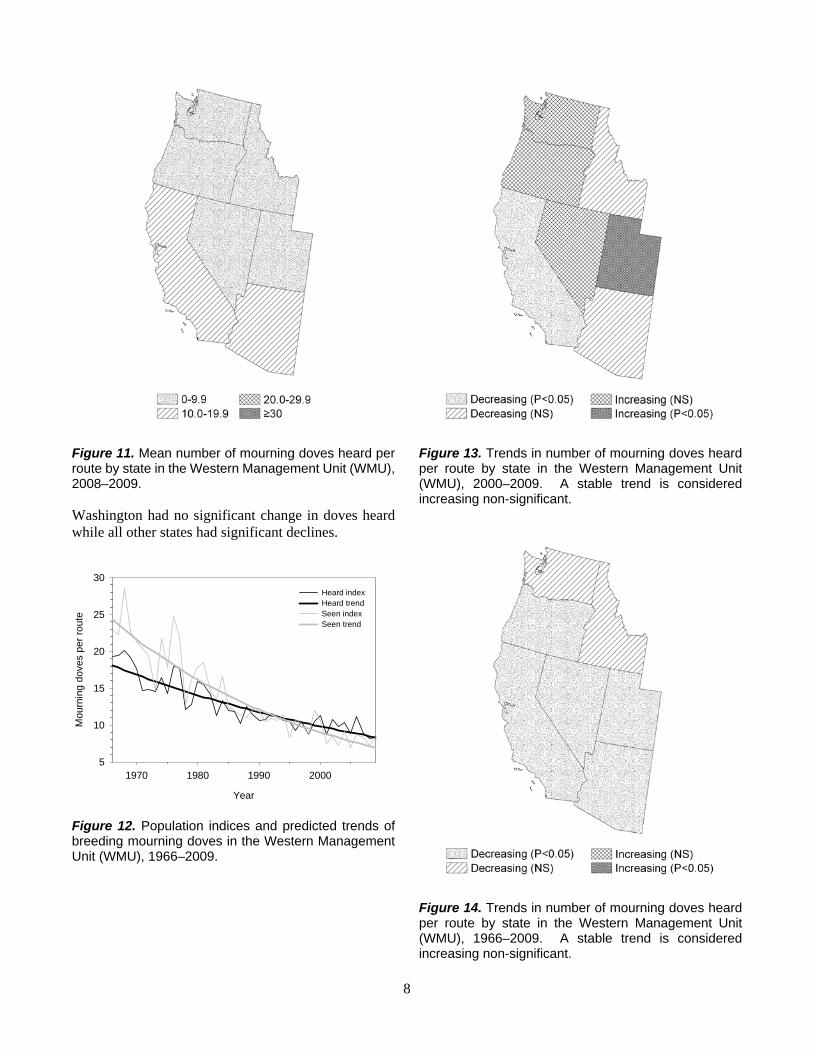
Figure 11. Mean number of mourning doves heard per route by state in the Western Management Unit (WMU), 2008–2009. Washington had no significant change in doves heard while all other states had significant declines.
Year
1970 1980 1990 2000
Mou
rnin
g do
ves
per r
oute
5
10
15
20
25
30Heard index Heard trend Seen index Seen trend
Figure 12. Population indices and predicted trends of breeding mourning doves in the Western Management Unit (WMU), 1966–2009.
Figure 13. Trends in number of mourning doves heard per route by state in the Western Management Unit (WMU), 2000–2009. A stable trend is considered increasing non-significant.
Figure 14. Trends in number of mourning doves heard per route by state in the Western Management Unit (WMU), 1966–2009. A stable trend is considered increasing non-significant.
8

9
BREEDING BIRD SURVEY RESULTS In general, trends indicated by the BBS, which records doves heard and seen together, tend to indicate fewer declines than the CCS, which analyzes doves heard and seen separately. The major differences occur in the EMU. This is likely due to the larger sample size of BBS survey routes and greater consistency of coverage by BBS than CCS routes in the unit (Sauer et al. 1994), although additional analyses are needed to clarify some differences in results between surveys within states. Comparisons below are from Table 3 in this report, and Table 1 (CCS results for doves heard) and Table 2 (CCS results for doves seen) in Dolton et al. (2008). Eastern Management Unit For the 10-year period, 1999–2008, the BBS showed that doves heard and seen increased significantly in the EMU while the CCS indicated no significant trend in either doves heard or seen. Over 43 years, 1966–2008, the BBS showed a significant increase while the CCS showed a significant decrease in doves heard and no significant trend in doves seen. Central Management Unit Over 10 years (1999–2008), there was a significant increase in doves heard and seen in the CMU according to BBS results. In contrast, CCS indicated doves heard decreased significantly, but there was no significant change in doves seen. For the 43-year period, both the BBS and CCS heard indicated significant declines while the CCS seen showed no significant trend. Western Management Unit There was no significant trend in doves heard and seen in the WMU indicated by the BBS over recent 10 and 43-year time periods. Similarly, there was no significant trend over the recent 10 years with the CCS for either doves heard or seen, but there was a significant decline for both doves heard and seen over 43 years. HARVEST SURVEY ESTIMATES Preliminary results of mourning dove harvest and hunter participation from HIP for the 2007 and 2008 hunting seasons are presented in Tables 5 and 6, respectively. The total estimated harvest for the 2008 season by Management Unit and for the U.S. are as follows:
Eastern: 7,671,800 ± 6%; Central: 7,520,000 ± 10%; Western: 2,210,700 ± 8%; and, U.S.: 17,402,400 ± 5%. Additional information about HIP, survey methodology, and results can be found in annual reports located at http://www.fws.gov/migratorybirds/newreportspublications/hip/hip.htm ACKNOWLEDGMENTS Personnel of state wildlife agencies and the U.S. Fish and Wildlife Service (USFWS) cooperated to collect the data presented in this report. Special thanks to state and regional Call-count Survey Coordinators including: T. Aldrich (UT DWR), R. Applegate (TN WRA), J. Austin (VT FWD), S. Baker (MS DWFP), T. Bogenschutz (IA DNR), M. Weaver (PA GC), R. Marshalla (IL DNR), B. Crose (OH DNR), M. DiBona (DE DNREC), J. Dickson (CT DEP), B. Dukes (SC DNR), L. Fendrick (OH DNR), K. Fothergill (CA DFG), V. Frawley (MI DNR), M. Frisbie (TX PWD), J. Fuller (NC WRC), J. Garris (NJ FW), E. Gorman (CO DNR), H. Hands (KS DWP), J. Hansen (MT FWP), B. Harvey (MD DNR), J. Knetter (ID DFG), K. Hodges (FL FWC), C. Huxoll (SD DGFP), D. Kraege (WA DFW), J. Lusk (NE GPC), D. McGowan (GA DNR), M. McInroy (IA DNR), T. Mitchusson (NM DGF), C. Mortimore (NV DW), M. Olinde (LA DWF), J. Richardson (OK DWC), J. Powers (AL DCNR), M. Rabe (AZ GFD), E. Robinson (NH FGD), R. Rothwell (WY GFD), D. Scarpitti (MA DFW), G. Sheridan (WY GFD), J. Schulz (MO DC), A. Stewart (MI DNR), N. Stricker (OH DNR), B. Swift (NY DEC), M. Szymanski (ND GFD), B. Tefft (RI DEM), B. Veverka (IN DFW), T. White (TN WRA), S. Wilson (WV DNR), and B. Bortner, H. Browers, A. Daisey, D. Davis, J. Dubovsky, C. Dwyer, T. Edwards, K. Frizzell, R. Ford, D. Haukos, D. James, S. Kelly, M. Mills, M. Strassburger, D. Viker, J. West, R. Wilson (USFWS). R. Rau (USFWS) developed and maintained the data entry website, provided guidance and historical perspective regarding Call-count Survey implementation, and provided assistance with data screening and management. K. Magruder (USFWS) provided assistance with data entry and management. R. Maruthalingam (USFWS) assisted in maintaining the website and developing data management applications for the Call-count Survey. J. R. Sauer (USGS) analyzed the data and provided statistical support. K. Richkus, H. Spriggs, S. Williams, and K. Wilkins (USFWS) provided the HIP data and explanation. M. Koneff, R. Rau and F. Rivera (USFWS) reviewed a draft of this report.

LITERATURE CITED Mirarchi, R.E. and T.S. Baskett. 1994. Mourning dove (Zenaida macroura). In A. Poole and F. Gill, editors, The birds of North America, No. 117. The Academy of Natural Sciences, Philadelphia and The American Ornithologists' Union, Washington, D.C., USA.
Aldrich, J.W. 1993. Classification and distribution.
Pages 47-54 in T.S. Baskett, M.W. Sayre, R.E. Tomlinson, and R.E. Mirarchi, Editors. Ecology and management of the mourning dove. Stackpole Books, Harrisburg, Pennsylvania, USA. Otis, D. L., J. H. Schulz, and D. P. Scott. 2008a.
Mourning dove (Zenaida macroura) harvest and population parameters derived from a national banding study. U.S. Department of Interior, Fish and Wildlife Service, Biological Technical Publication FWS/BTP-R3010-2008, Washington, D.C., USA/
Dolton, D.D. 1993. The call-count survey: historic development and current procedures. Pages 233–252 in T.S. Baskett, M.W. Sayre, R.E. Tomlinson, and R.E. Mirarchi, editors. Ecology and management of the mourning dove. Stackpole Books, Harrisburg, Pennsylvania, USA.
Otis, D. L., J. H. Schulz, D. A. Miller, R. Mirarchi, and T. Baskett. 2008b. Mourning dove (Zenaida macroura). In The Birds of North America, No. 117. (A. Poole and F. Gill, editors.). Philadelphia: The Academy of Natural Sciences; Washington, D.C., USA.
Dolton, D.D., R.D. Rau, and K. Parker. 2008. Mourning dove breeding population status, 2008. U.S. Fish and Wildlife Service, Laurel, Maryland, USA.
Fenneman, N.M. 1931. Physiography of western United States. McGraw Hill Book Co., New York. 534 pp.
Peterjohn, B.G., J.R. Sauer and W.A. Link. 1994. The 1992 and 1993 summary of the North American breeding bird survey. Bird Populations 2:46–61.
Geissler, P.H. and J.R. Sauer. 1990. Topics in route regression analysis. Pages 54–57 in J.R. Sauer and S. Droege, editors. Survey designs and statistical methods for the estimation of avian population trends. U.S. Fish and Wildlife Service, Biological Report 90(1).
Sauer, J.R. and P.H. Geissler. 1990. Annual indices from route regression analyses. Pages 58–62 in J.R. Sauer and S. Droege, eds. Survey designs and statistical methods for the estimation of avian population trends. U.S. Fish and Wildlife Service, Biological Report. 90(1).
Kiel, W.H. 1959. Mourning dove management units, a progress report. U.S. Fish and Wildlife Service, Special Scientific Report—Wildlife 42.
Sauer, J.R., D.D. Dolton, and S. Droege. 1994.Mourning dove population trend estimates from Call-count and North American Breeding Bird Surveys. Journal of Wildlife Management. 58(3):506–515.
Kiel, W.H. 1961. The mourning dove program for the future. Transactions of the North American Wildlife and Natural Resources Conference 26:418–435.
Link, W.A. and J.R. Sauer. 1994. Estimating equations estimates of trends. Bird Populations 2:23–32.
U.S. Department of the Interior. 1988. Final Supplemental Environmental Impact Statement: Issuance of annual regulations permitting the sport hunting of migratory birds. U.S. Fish and Wildlife Service. Washington, D.C., USA.
McClure, H.E. 1939. Cooing activity and censusing of the mourning dove. Journal of Wildlife Management 3:323–328.
10

11
Table 1. Trends (% changea per year as determined by linear regression) in number of mourning doves heard along Call-count Survey routes, 1966–2009. Management Unit 2 year (2008–2009b) 10 year (2000–2009) 44 year (1966–2009) State N % changec 90% CI N % changec 90% CI N % changec 90% CI Eastern 366 1.5 -3.9 6.9 469 -0.4 -1.0 0.3 620 -0.3 * -0.6 0.0 Hunt states 299 4.8 -1.2 10.8 380 -0.6 -1.3 0.1 479 -0.5 *** -0.8 -0.2 AL 25 0.4 -15.9 16.8 30 -1.5 -3.8 0.9 45 -0.7 * -1.3 -0.1 DE-MD 13 19.7 -15.3 54.7 15 2.1 -0.1 4.3 20 -0.5 -1.9 0.9 FL 20 -17.2 -42.2 7.8 24 -2.9 -6.4 0.6 29 -0.7 -1.5 0.2 GA 19 21.5 * -2.8 45.8 23 2.6 -0.1 5.3 31 -0.9 ** -1.6 -0.2 IL 12 13.5 -8.0 35.0 21 -0.9 -3.1 1.4 23 0.2 -0.9 1.3 IN 13 8.4 -13.8 30.7 15 0.4 -3.0 3.9 18 -1.2 * -2.2 -0.2 KY 17 11.7 -4.7 28.0 20 -0.6 -1.7 0.5 26 -0.4 -1.4 0.7 LA 18 30.8 * -0.2 61.8 19 0.5 -1.8 2.7 23 1.2 * 0.0 2.3 MS 15 -5.0 -27.1 17.2 23 -1.9 -4.0 0.2 32 -1.6 * -3.2 0.0 NC 19 -1.2 -10.7 8.2 22 0.4 -1.5 2.2 25 0.3 -0.5 1.0 OH 32 2.8 -17.4 22.9 37 0.0 -1.7 1.6 57 -1.1 *** -1.7 -0.4 PA 14 7.9 -6.9 22.7 20 0.2 -3.0 3.3 20 1.0 -0.3 2.3 SC 16 1.2 -11.2 13.5 21 -1.6 -3.8 0.7 27 -1.2 ** -2.0 -0.3 TN 16 41.5 *** 10.6 72.5 25 -2.1 -4.3 0.1 35 -1.6 *** -2.6 -0.7 VA 23 13.6 -9.4 36.5 32 0.3 -3.3 3.9 33 -1.7 * -3.2 -0.2 WI 17 -9.7 -35.3 16.0 22 -0.3 -2.7 2.2 23 0.9 -0.2 2.0 WV 10 -5.6 -27.5 16.3 11 3.3 -0.2 6.8 12 1.6 0.0 3.3 Nonhunt states 67 -13.9 ** -25.7 -2.1 89 0.7 -1.2 2.7 141 1.1 * 0.1 2.1 MI 17 -19.9 ** -35.4 -4.4 19 1.9 -1.1 4.9 23 1.1 -0.5 2.6 N. Englandd 29 7.6 -11.7 27.0 42 -2.9 *** -4.4 -1.3 76 0.9 ** 0.2 1.6 NJ 11 28.0 -26.7 82.8 11 -2.0 -4.3 0.3 20 -2.0 -4.5 0.4 NY 10 -6.3 -27.5 14.9 17 1.2 -1.6 3.9 22 2.3 * 0.0 4.5
Central 303 10.1 ** 1.5 18.8 406 -2.6 *** -3.3 -1.9 551 -0.8 *** -1.2 -0.5 AR 13 2.0 -28.6 32.6 18 1.1 -1.1 3.4 21 -0.8 -1.9 0.3 CO 11 -16.7 -37.9 4.4 16 1.4 -2.6 5.4 21 -0.9 * -1.6 -0.1 IA 15 -9.1 -35.5 17.4 17 2.1 -0.5 4.8 19 0.3 -0.6 1.2 KS 20 9.0 -11.0 29.0 28 1.1 -1.1 3.4 36 0.0 -0.7 0.8 MN 9 0.5 -24.3 25.4 12 -0.8 -6.4 4.7 13 -2.0 ** -3.4 -0.6 MO 14 3.5 -22.1 29.0 20 0.3 -2.1 2.6 28 -2.1 *** -3.4 -0.9 MT 17 -3.9 -31.2 23.3 20 -1.4 -5.8 3.0 29 -1.7 * -3.3 -0.1 NE 17 21.8 -9.4 52.9 24 -2.8 *** -4.2 -1.4 28 -1.1 *** -1.7 -0.5 NM 19 28.1 * -1.3 57.5 28 3.9 * 0.3 7.5 31 1.4 ** 0.4 2.4 ND 20 -7.1 -26.6 12.3 27 -3.5 *** -5.0 -2.0 31 -0.8 -1.8 0.2 OK 12 52.9 ** 4.1 101.7 16 -0.9 -3.4 1.6 25 0.1 -2.6 2.8 SD 18 -31.5 ** -58.6 -4.5 22 -0.6 -2.9 1.8 30 -0.7 -1.9 0.4 TX 106 33.4 *** 16.0 50.9 139 -4.7 *** -5.9 -3.4 213 -1.1 *** -1.7 -0.4 WY 12 -35.6 *** -50.5 -20.6 19 -4.5 -9.4 0.5 26 -2.4 ** -4.3 -0.5
Western 139 2.6 -13.7 18.8 213 -1.0 -2.2 0.2 291 -1.8 *** -2.3 -1.3 AZ 27 -10.8 -43.4 21.8 50 -0.8 -3.3 1.8 71 -0.9 ** -1.6 -0.1 CA 40 0.3 -16.4 17.1 60 -2.5 *** -4.0 -1.1 84 -2.4 *** -3.4 -1.4 ID 16 -12.2 -49.1 24.7 23 -0.1 -3.8 3.5 29 -0.7 -2.0 0.5 NV 17 30.9 -15.5 77.4 21 0.0 -5.1 5.1 34 -3.2 *** -4.9 -1.4 ORe 10 22.2 * -2.5 46.9 20 2.1 -2.8 7.0 25 -1.5 ** -2.7 -0.3 UT 13 62.0 -34.7 158.7 16 5.7 ** 1.8 9.5 20 -3.6 ** -6.1 -1.2 WA 16 27.2 * -1.5 55.9 23 0.7 -2.1 3.4 28 -1.9 * -3.8 0.0
a Mean of route trends weighted by land area and population density. The estimated count in the next year is (%/100+1) times the count in the current year where % is the annual change. Note: extrapolating the estimated trend statistic (% change per year) over time (e.g., 44 years) may exaggerate the total change over the period.
b The 2-year trend is the best estimate of the change between 2008 and 2009. This is because only data from comparable routes (those run by the same observer in both years) are used in the analysis. This change will differ from the change calculated from 2008 to 2009 using the annual indices because the index values are less precise, as they incorporate data from routes not surveyed in both years. The 2-year trend is useful in evaluating short-term change; however, the long-term trend is more relevant to management decision-making.
c *=P<0.1, **=P<0.05, and ***=P<0.01. For purposes of this report, statistical significance was defined as P<0.05, except for the 2-year comparison where P<0.10 was used because of the low power of the test.
d New England consists of CT, ME, MA, NH, RI, and VT; RI is a hunt state but was included in this group for purposes of analysis. e Due to small sample sizes within Oregon strata, a pooled estimate amongst strata is provided for Oregon for the 2-year trend.

12
Table 2. Trends (% changea per year as determined by linear regression) in number of mourning doves seen along Call-count Survey routes, 1966–2009. Management Unit 10 year (2000–2009) 44 year (1966–2009) State N % changeb 90% CI N % changeb 90% CI Eastern 467 -0.7 -1.5 0.1 615 0.3 -0.2 0.9 Hunt states 380 -0.9 * -1.7 0.0 477 0.1 -0.4 0.7 AL 30 -2.7 -6.2 0.7 45 -1.3 ** -2.4 -0.3 DE-MD 15 -1.8 -4.7 1.1 20 0.3 -0.7 1.4 FL 25 -1.3 -4.1 1.5 29 3.3 *** 2.1 4.4 GA 23 1.2 -3.9 6.2 31 0.5 -0.7 1.7 IL 21 -0.4 -2.4 1.6 23 -0.8 -2.2 0.6 IN 15 -2.9 -7.6 1.8 18 -1.8 -4.6 1.0 KY 20 -2.2 -5.5 1.1 24 1.2 -0.1 2.6 LA 18 0.2 -1.1 1.4 23 2.1 *** 1.3 2.9 MS 23 0.7 -1.1 2.6 32 -1.2 -3.1 0.8 NC 22 3.4 ** 0.8 6.0 25 -0.1 -1.1 0.9 OH 37 -2.5 * -4.7 -0.4 57 0.6 -0.8 1.9 PA 20 -3.2 * -6.3 -0.2 20 0.8 -0.7 2.4 SC 21 3.6 -1.0 8.1 27 1.5 ** 0.3 2.6 TN 25 -0.9 -2.7 0.9 35 -0.7 -1.7 0.2 VA 33 -0.3 -5.3 4.7 33 -0.4 -2.4 1.7 WI 21 3.8 * 0.6 7.0 23 2.9 *** 1.8 4.1 WV 11 -2.2 -8.8 4.4 12 3.3 *** 1.6 5.1 Nonhunt states 87 0.0 -2.0 2.1 138 2.0 *** 1.1 2.9 MI 19 0.6 -2.2 3.3 23 2.1 *** 1.0 3.3 N. Englandc 40 -2.4 -5.0 0.2 73 1.6 -0.1 3.2 NJ 11 3.7 * 0.5 6.9 20 -0.6 -2.2 1.0 NY 17 -0.8 -5.4 3.7 22 2.8 * 0.2 5.3
Central 402 0.2 -1.0 1.3 549 0.0 -0.4 0.4 AR 18 1.9 -0.6 4.4 21 -1.0 ** -1.7 -0.3 CO 15 -3.0 -6.0 0.0 20 -0.6 -2.0 0.7 IA 17 1.1 -2.8 4.9 19 0.5 -0.8 1.9 KS 28 2.3 * 0.3 4.3 36 -0.3 -1.1 0.4 MN 12 0.2 -7.0 7.5 14 -0.9 -2.8 0.9 MO 20 0.0 -1.9 1.9 28 -3.0 *** -4.8 -1.1 MT 20 7.1 -2.0 16.3 29 1.8 * 0.1 3.4 NE 24 0.7 -2.0 3.3 28 -0.5 -2.0 0.9 NM 28 7.7 *** 6.5 9.0 31 0.9 -1.5 3.3 ND 27 -3.0 -6.2 0.1 31 -0.4 -1.3 0.5 OK 16 0.5 -2.2 3.3 25 0.3 -0.8 1.3 SD 22 1.2 -1.7 4.0 30 -1.0 -2.2 0.3 TX 139 -0.4 -2.2 1.4 213 0.6 * 0.0 1.1 WY 16 -3.7 -9.1 1.7 24 -3.3 ** -6.0 -0.6
Western 202 -0.9 -2.7 0.9 287 -2.9 *** -3.7 -2.1 AZ 45 -3.7 * -7.0 -0.4 72 -3.9 *** -5.7 -2.2 CA 58 -2.9 *** -4.6 -1.2 84 -2.4 *** -3.4 -1.4 ID 22 8.0 *** 3.0 13.0 29 -2.0 -4.6 0.5 NV 20 6.0 -2.7 14.7 34 -1.2 -4.2 1.7 OR 19 4.3 -5.5 14.0 23 -4.4 *** -6.7 -2.1 UT 15 5.3 * 0.2 10.4 20 -4.9 ** -8.7 -1.2 WA 23 0.3 -5.6 6.1 25 0.7 -1.6 3.1
a Mean of route trends weighted by land area and population density. The estimated count in the next year is (%/100+1) times the count in the current year where % is the annual change. Note: extrapolating the estimated trend statistic (% change per year) over time (e.g., 44 years) may exaggerate the total change over the period.
b *=P<0.1, **=P<0.05, and ***=P<0.01. For purposes of this report, statistical significance was defined as P<0.05, except for the 2-year comparison where P<0.10 was used because of the low power of the test.
c New England consists of CT, ME, MA, NH, RI, and VT; RI is a hunt state but was included in this group for purposes of analysis.

13
Table 3. Trends (% changea per year as determined by linear regression) in number of mourning doves heard and seen along Breeding Bird Survey routes, 1966–2008. Management Unit 10 year (1999–2008) 43 year (1966–2008) State N % changeb 90% CI N % changeb 90% CI Eastern 1375 0.7 *** 0.3 1.0 1664 0.4 *** 0.2 0.7 Hunt states 1069 1.0 *** 0.6 1.5 1269 0.3 0.0 0.5 AL 90 -0.7 -1.9 0.5 103 -1.3 *** -1.9 -0.6 DE-MD 67 -1.6 *** -2.5 -0.7 79 0.1 -0.3 0.6 FL 72 -1.8 -3.7 0.1 87 1.4 *** 0.8 2.1 GA 67 -1.1 -2.9 0.6 83 -1.6 *** -2.5 -0.7 IL 100 5.1 *** 3.8 6.4 102 1.2 *** 0.6 1.9 IN 55 1.8 *** 0.8 2.8 61 0.3 -0.1 0.7 KY 41 0.9 -0.6 2.4 58 0.5 -0.2 1.2 LA 55 1.2 -0.4 2.8 75 2.2 *** 1.0 3.4 MS 30 1.7 -0.5 3.8 39 -1.7 *** -2.5 -0.8 NC 75 1.9 *** 1.0 2.8 88 0.3 -0.4 1.1 OH 58 -0.1 -1.4 1.3 78 0.8 ** 0.3 1.3 PA 98 -0.7 -1.6 0.3 122 1.6 *** 1.1 2.2 SC 31 1.4 -1.5 4.2 39 -0.1 -0.9 0.7 TN 41 -1.6 -3.2 0.1 47 -0.7 -1.4 0.0 VA 47 -1.1 -3.0 0.9 55 -0.8 ** -1.3 -0.2 WI 93 2.4 *** 1.7 3.1 96 1.6 *** 1.0 2.3 WV 49 -0.1 -1.9 1.7 57 4.7 *** 4.0 5.4 Nonhunt states 306 -1.4 *** -2.0 -0.8 395 1.6 *** 1.2 2.0 MI 60 1.0 * 0.1 1.9 85 0.7 ** 0.2 1.3 N. Englandc 125 -4.1 *** -5.1 -3.1 155 2.3 *** 1.7 2.9 NJ 25 -1.1 -3.3 1.2 37 0.2 -0.9 1.3 NY 96 -1.0 -2.2 0.1 118 2.4 *** 2.0 2.8
Central 900 0.9 ** 0.3 1.6 1060 -0.4 *** -0.6 -0.1 AR 30 -0.4 -2.2 1.4 35 0.9 -0.2 2.1 CO 119 3.5 *** 1.7 5.4 134 1.2 * 0.2 2.1 IA 33 3.5 *** 1.5 5.5 39 -0.3 -1.3 0.6 KS 62 2.5 * 0.2 4.8 63 0.0 -0.7 0.8 MN 61 0.0 -2.4 2.5 72 -0.9 * -1.8 -0.1 MO 51 1.3 -0.3 2.8 66 -1.4 *** -2.2 -0.6 MT 45 -0.7 -3.2 1.7 53 -0.7 -1.5 0.0 NE 46 4.2 ** 0.9 7.5 49 -0.2 -1.0 0.7 NM 61 -0.8 -3.1 1.6 74 -0.1 -1.0 0.9 ND 42 -1.5 -3.6 0.7 47 0.4 -0.3 1.1 OK 53 -0.7 -2.2 0.8 60 -1.2 *** -1.8 -0.6 SD 43 -0.4 -3.0 2.1 52 0.4 -0.4 1.2 TX 180 -0.8 -2.1 0.5 209 -1.3 *** -1.8 -0.8 WY 74 1.6 -0.4 3.6 107 0.7 -0.9 2.4
Western 503 0.8 -0.7 2.2 647 -0.7 -1.4 0.0 AZ 56 1.0 -2.9 4.9 78 0.3 -2.4 3.0 CA 162 1.0 -0.2 2.3 226 -0.9 * -1.7 -0.1 ID 39 2.1 -1.2 5.4 43 -0.3 -1.3 0.7 NV 25 -3.6 ** -6.1 -1.1 36 1.2 -0.2 2.6 OR 77 0.5 -2.6 3.6 103 -1.8 ** -3.0 -0.6 UT 86 0.8 -1.7 3.3 95 -1.5 *** -2.4 -0.6 WA 58 1.2 -0.7 3.2 66 0.4 -0.6 1.3
a Mean of route trends weighted by land area and population density. The estimated count in the next year is (%/100+1) times the count in the current year where % is the annual change. Note: extrapolating the estimated trend statistic (% change per year) over time (e.g., 44 years) may exaggerate the total change over the period.
b *=P<0.1, **=P<0.05, and ***=P<0.01. For purposes of this report, statistical significance was defined as P<0.05, except for the 2-year comparison where P<0.10 was used because of the low power of the test.
c New England consists of CT, ME, MA, NH, RI, and VT; RI is a hunt state but was included in this group for purposes of analysis.

14
Table 4. Breeding population indicesa based on mourning doves heard along Call-count routes, 1966–2009. Management Unit Year State 1966 1967 1968 1969 1970 1971 1972 1973 1974 1975 Eastern 19.9 19.0 17.7 17.7 18.3 18.6 19.1 17.6 17.4 18.2 Hunt states 22.5 21.1 20.3 20.3 21.1 20.2 20.8 19.2 19.6 19.8 AL 25.8 23.0 20.7 21.0 21.3 17.5 25.0 21.8 16.6 21.1 DE-MD 13.9 17.3 12.1 12.9 16.0 13.8 15.1 15.0 16.3 11.7 FL 13.4 12.8 10.9 11.5 14.6 12.2 12.5 12.6 14.8 15.1 GA 29.6 27.7 23.8 25.5 32.2 25.4 24.2 26.7 27.7 30.1 IL 24.0 20.7 24.6 21.4 24.5 22.4 23.0 22.5 19.1 26.3 IN 35.9 33.1 32.6 31.7 30.7 41.5 36.4 32.6 31.2 33.0 KY 24.0 21.7 21.2 22.2 26.7 23.9 20.1 23.9 27.7 19.5 LA 10.2 10.4 9.8 11.4 7.1 10.2 11.3 8.8 10.3 10.7 MS 39.6 34.0 28.8 26.6 29.6 30.2 33.6 30.1 24.3 25.8 NC 34.4 27.8 29.4 42.2 48.8 28.5 23.1 44.0 25.1 14.2 OH 24.7 23.3 21.1 24.0 23.7 24.6 25.6 20.4 24.8 37.9 PA 8.9 9.5 8.8 8.4 5.5 6.4 8.9 5.8 8.6 6.0 SC 33.6 36.7 37.3 36.0 33.9 29.7 26.3 30.1 28.0 27.7 TN 33.6 24.5 25.2 24.8 33.7 23.8 30.0 22.8 24.4 23.3 VA 24.7 20.7 23.5 20.8 26.5 21.5 12.8 15.1 20.8 23.2 WI 10.0 12.9 13.0 9.9 10.8 15.6 16.4 10.9 11.5 14.6 WV 6.5 5.5 5.6 6.0 5.6 5.1 6.7 3.9 4.2 2.4 Nonhunt states 9.0 9.4 7.6 7.4 7.6 10.6 10.7 10.1 8.5 10.5 MI 12.7 13.8 9.1 9.3 7.5 14.9 15.8 12.8 10.9 12.3 N. Englandb 6.5 7.0 6.4 5.4 6.3 6.6 7.3 8.5 5.3 5.0 NJ 20.5 17.5 21.7 20.0 27.0 25.5 26.7 23.6 23.3 16.7 NY 5.9 5.9 5.6 5.6 6.9 8.1 6.4 6.7 6.9 12.5
Central 31.5 28.3 29.1 27.7 26.8 26.2 29.8 24.8 27.8 27.1 AR 22.0 23.0 22.0 21.2 22.9 23.0 21.5 24.3 22.3 21.5 CO 24.2 23.8 21.7 29.6 29.6 21.5 27.3 16.9 26.8 19.7 IA 31.0 27.9 30.3 27.3 19.8 24.3 32.8 30.9 24.7 23.0 KS 46.7 48.1 49.9 50.6 46.6 47.5 53.1 47.2 46.9 44.9 MN 33.5 26.7 28.7 21.2 16.7 24.0 27.7 20.9 29.0 31.5 MO 40.4 38.1 47.7 28.8 39.8 33.4 45.2 33.9 29.0 33.9 MT 28.6 26.5 20.8 23.0 18.4 26.1 20.8 14.9 17.4 23.8 NE 46.1 40.4 51.5 50.3 48.6 46.0 44.0 42.1 43.6 41.0 NM 12.6 9.3 13.1 10.0 9.9 9.4 10.8 7.8 9.6 12.1 ND 43.2 41.1 56.2 46.6 41.1 41.9 43.4 47.2 45.1 32.5 OK 19.6 24.2 28.6 28.8 21.7 16.6 27.2 25.6 27.0 24.4 SD 54.8 34.3 46.9 39.9 47.4 41.7 41.4 43.7 52.2 44.1 TX 29.7 24.6 23.9 21.5 23.4 22.2 29.6 23.3 24.4 21.9 WY 24.6 25.7 13.6 22.3 21.5 12.3 17.0 17.0 24.3 21.6
Western 19.3 19.5 20.2 19.2 17.7 14.7 14.8 14.5 16.5 14.3 AZ 28.5 28.7 25.6 30.6 30.7 20.7 23.3 28.2 24.5 26.9 CA 28.9 27.3 25.2 25.0 24.2 18.2 22.2 21.3 23.1 19.5 ID 12.8 13.0 12.3 13.4 12.4 10.2 9.7 12.4 10.9 7.6 NV 10.5 9.8 23.4 16.9 12.1 7.4 10.0 7.1 9.6 6.3 OR 14.2 9.5 11.2 10.2 7.8 6.9 6.8 6.8 12.0 9.2 UT 24.0 36.7 18.5 17.5 20.4 28.6 16.6 14.4 16.4 17.5 WA 11.8 17.4 16.3 13.0 13.2 15.7 11.2 10.3 13.0 14.2
a Annual indices are the predicted value from the trend analysis plus the deviation from the expected value in a year. Large but nonsignificant changes due to small sample sizes produce exaggerated indices over the 44-year period.
b New England consists of CT, ME, MA, NH, RI, and VT; RI is a hunt state but was included in this group for purposes of analysis.

15
Table 4. Continued. Management Unit Year State 1976 1977 1978 1979 1980 1981 1982 1983 1984 1985 Eastern 17.8 19.1 17.1 15.4 17.7 18.6 18.1 17.2 15.5 16.4 Hunt states 19.9 21.5 18.5 17.7 19.0 19.9 19.9 18.9 16.9 17.9 AL 20.3 22.4 24.5 23.6 23.6 22.5 22.9 23.0 19.2 24.5 DE-MD 14.6 13.4 14.4 14.1 13.5 12.9 13.6 9.7 11.2 12.4 FL 14.0 15.3 12.0 13.0 10.3 9.1 10.6 12.4 8.4 10.8 GA 23.7 24.7 27.2 23.8 24.2 26.8 28.8 25.8 21.0 26.8 IL 25.8 27.6 21.1 18.4 18.8 21.1 25.7 26.4 21.4 18.4 IN 33.4 37.5 20.3 21.6 27.4 31.7 22.6 19.5 21.2 18.7 KY 24.5 23.0 24.6 16.9 16.4 27.9 24.0 13.4 21.5 22.4 LA 10.8 8.9 10.5 8.9 12.4 10.6 13.3 12.3 11.7 10.5 MS 26.3 27.1 30.7 26.3 25.0 25.1 31.7 26.6 19.6 25.9 NC 17.4 47.0 25.1 29.8 28.9 28.4 24.0 28.3 31.8 22.1 OH 27.6 26.4 14.0 13.6 16.3 19.8 18.8 20.0 18.7 17.5 PA 6.0 4.9 6.1 6.7 8.0 9.6 9.1 9.0 8.3 9.1 SC 27.4 23.3 30.8 26.1 32.8 31.9 32.9 31.3 28.4 28.5 TN 23.0 25.2 31.2 21.3 23.1 19.6 26.2 20.3 17.4 22.3 VA 22.4 29.9 22.1 19.5 18.9 16.3 18.0 18.0 17.6 16.5 WI 14.7 19.4 7.8 11.5 14.8 19.9 11.2 13.1 10.3 10.7 WV 6.1 5.8 6.5 7.3 8.5 6.8 6.5 6.2 5.4 6.7 Nonhunt states 8.9 9.7 10.2 7.1 11.2 11.9 10.2 9.8 9.3 9.8 MI 12.5 10.8 12.4 7.3 13.6 15.6 11.4 10.1 10.9 12.1 N. Englandb 4.7 8.7 7.3 6.0 7.5 9.0 7.4 7.9 6.7 7.4 NJ 21.0 23.0 18.2 19.4 18.1 14.8 17.1 20.4 12.9 13.0 NY 7.4 7.4 9.0 6.1 11.0 9.2 10.0 9.3 9.3 8.4
Central 27.8 26.5 26.0 25.5 28.6 27.8 27.6 24.4 22.8 24.8 AR 26.1 21.3 15.0 12.2 20.2 22.1 25.7 19.3 13.7 13.6 CO 27.9 25.8 28.5 23.6 27.3 30.9 29.9 16.5 20.6 24.5 IA 28.2 21.9 24.7 21.0 28.4 31.5 22.7 16.1 23.7 26.2 KS 49.4 46.9 36.8 53.7 58.7 56.1 53.5 60.3 47.7 61.9 MN 27.3 31.4 30.2 30.8 33.1 29.2 25.6 22.3 18.9 20.5 MO 30.0 34.8 22.2 21.1 33.0 27.8 24.4 23.6 22.5 21.4 MT 17.2 21.1 20.3 20.2 18.5 17.3 22.2 17.8 13.5 18.7 NE 46.2 46.6 38.2 40.9 51.9 49.3 48.0 43.7 41.6 42.7 NM 11.9 10.7 10.8 7.4 12.2 12.1 9.5 13.0 14.1 12.2 ND 52.1 42.8 45.2 42.0 47.3 47.3 44.2 42.1 32.7 42.6 OK 25.8 33.2 25.5 24.8 25.8 25.6 26.8 27.5 20.5 20.0 SD 47.4 41.4 44.6 43.6 43.7 39.3 46.8 40.3 44.8 42.1 TX 21.3 20.3 21.1 26.0 24.7 22.3 21.4 19.7 19.3 19.9 WY 20.2 12.8 20.9 16.4 14.8 16.3 21.1 14.4 13.1 15.4
Western 17.9 17.9 12.1 12.8 15.9 15.6 14.2 11.3 13.3 12.0 AZ 27.8 25.0 25.1 24.5 22.0 24.8 28.4 22.1 27.2 21.9 CA 23.3 17.9 16.1 12.5 21.2 17.6 21.7 13.4 18.6 13.2 ID 14.0 17.1 9.6 9.4 10.1 11.2 11.6 9.3 11.0 10.2 NV 10.3 10.6 6.3 9.3 13.7 10.0 5.7 5.1 5.1 6.5 OR 9.6 10.9 5.9 6.1 9.2 7.9 7.7 6.0 7.6 8.4 UT 20.2 23.7 10.5 12.8 15.4 20.4 11.0 12.4 13.8 9.1 WA 13.7 15.0 9.7 13.7 9.4 11.4 10.6 9.0 7.9 9.9
a Annual indices are the predicted value from the trend analysis plus the deviation from the expected value in a year. Large but nonsignificant changes due to small sample sizes produce exaggerated indices over the 44-year period.
b New England consists of CT, ME, MA, NH, RI, and VT; RI is a hunt state but was included in this group for purposes of analysis.
16
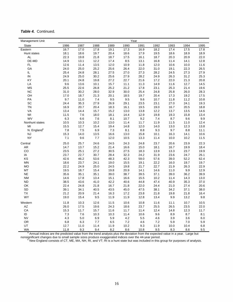
Table 4. Continued. Management Unit Year State 1986 1987 1988 1989 1990 1991 1992 1993 1994 1995 Eastern 16.7 17.0 17.8 19.1 17.3 16.9 18.2 17.4 17.5 17.8 Hunt states 18.1 18.6 19.7 20.4 18.6 17.9 19.5 18.6 18.9 18.9 AL 22.3 19.8 21.8 18.7 17.5 16.1 18.7 20.3 20.9 22.0 DE-MD 14.9 13.1 12.2 17.4 8.5 13.1 16.8 11.4 14.1 12.8 FL 12.6 11.4 13.5 12.0 10.9 11.8 12.0 10.6 10.0 11.6 GA 24.0 25.0 25.2 25.6 26.4 22.0 31.0 19.1 22.3 26.5 IL 25.4 24.8 28.1 27.5 27.0 27.3 28.2 24.5 27.3 27.9 IN 24.9 25.0 30.2 25.6 27.9 28.2 24.9 26.3 31.2 25.3 KY 20.1 24.8 19.8 27.2 22.7 21.6 17.2 22.0 21.3 20.8 LA 9.6 13.6 10.1 15.7 11.1 11.3 14.9 11.6 12.7 14.5 MS 25.5 22.6 26.8 25.2 21.2 17.8 23.1 25.3 21.4 19.6 NC 31.0 30.2 28.0 32.9 30.0 25.4 24.8 25.8 26.0 28.3 OH 17.0 18.7 21.3 20.1 18.5 19.7 20.4 17.3 19.2 17.5 PA 9.7 11.0 7.4 9.5 9.5 9.6 10.7 11.8 11.2 10.8 SC 24.4 35.3 27.9 26.9 29.1 23.5 23.1 27.0 24.1 19.3 TN 16.9 20.7 20.4 18.3 16.1 19.5 19.0 16.7 20.5 18.8 VA 13.4 14.4 15.7 15.2 13.0 13.8 12.2 13.7 13.5 14.6 WI 11.5 7.6 18.0 18.1 14.4 12.9 19.8 19.3 15.8 13.4 WV 6.3 6.6 7.6 8.1 10.7 9.2 7.4 8.7 9.6 9.9 Nonhunt states 10.5 10.3 10.2 13.0 11.4 11.7 11.9 11.5 11.0 12.4 MI 15.5 12.7 15.4 19.4 14.8 12.0 14.0 13.0 12.3 13.8 N. Englandb 7.8 7.5 6.9 7.3 8.1 8.8 9.3 9.7 8.8 11.1 NJ 15.3 14.0 13.5 16.6 13.0 15.8 10.1 16.3 14.1 10.6 NY 7.1 9.6 7.7 12.0 10.5 13.3 11.4 10.0 10.2 11.5
Central 25.0 25.7 24.6 24.5 24.3 24.8 23.7 20.6 23.9 22.3 AR 14.7 13.7 15.2 21.4 16.6 15.0 18.1 16.7 19.9 18.4 CO 23.5 25.1 27.2 30.5 27.5 18.3 13.9 13.3 23.7 19.9 IA 23.7 22.7 30.7 28.4 32.3 24.2 31.9 23.6 24.7 26.1 KS 42.6 46.2 53.6 48.3 42.3 59.0 57.6 39.0 52.2 62.4 MN 18.6 23.7 24.1 19.0 15.5 19.1 22.2 16.0 19.7 19.7 MO 22.2 24.9 25.0 24.5 19.8 21.7 22.7 21.9 26.3 22.9 MT 19.5 18.7 15.4 19.8 20.9 14.1 14.6 11.0 9.9 12.9 NE 35.6 35.1 35.1 39.0 38.7 39.5 37.1 39.0 36.2 39.9 NM 14.6 17.8 13.4 15.1 16.6 15.5 10.2 11.4 14.3 13.0 ND 38.5 43.6 41.0 42.2 40.6 44.8 47.4 40.9 35.3 37.0 OK 22.4 24.8 21.8 16.7 21.8 22.0 24.4 21.0 27.4 20.6 SD 39.1 34.1 40.5 43.5 45.0 47.5 38.1 34.2 37.1 38.0 TX 21.2 20.9 21.4 16.3 17.2 23.8 21.8 19.8 21.8 16.4 WY 19.0 15.4 9.5 11.9 11.9 12.8 13.4 9.9 13.2 9.8
Western 11.8 10.3 12.6 11.5 10.6 10.8 11.6 11.1 10.7 10.5 AZ 26.0 17.5 19.6 24.3 18.6 23.7 25.5 26.5 23.5 22.0 CA 15.3 11.7 15.7 11.6 11.7 11.4 12.4 14.8 12.3 11.7 ID 7.3 7.6 10.3 10.3 11.4 10.6 9.6 8.9 8.7 8.1 NV 4.3 5.0 6.9 5.9 4.2 5.5 4.6 3.9 3.6 6.0 OR 6.8 6.3 7.7 6.5 7.2 4.6 7.2 5.9 7.0 5.9 UT 12.7 11.0 11.4 11.9 10.2 9.3 11.9 10.0 10.4 6.8 WA 11.8 9.3 9.4 8.2 8.6 10.8 9.5 8.3 8.6 9.5
a Annual indices are the predicted value from the trend analysis plus the deviation from the expected value in a year. Large but nonsignificant changes due to small sample sizes produce exaggerated indices over the 44-year period.
b New England consists of CT, ME, MA, NH, RI, and VT; RI is a hunt state but was included in this group for purposes of analysis.

17
Table 4. Continued. Management Unit Year State 1996 1997 1998 1999 2000 2001 2002 2003 2004 2005 Eastern 15.5 15.6 16.3 17.5 18.4 16.6 16.2 16.5 15.8 16.7 Hunt states 16.3 16.5 17.3 18.3 19.1 17.5 16.7 17.3 16.7 17.5 AL 16.9 16.0 17.8 17.1 18.3 17.3 20.3 15.6 17.8 17.7 DE-MD 12.1 10.1 14.0 10.0 9.6 9.6 8.1 13.1 13.6 12.4 FL 10.8 10.0 12.3 12.8 12.4 8.8 9.7 10.3 9.8 10.8 GA 22.3 19.2 18.4 18.7 16.5 22.9 12.5 19.9 18.7 20.5 IL 22.0 22.5 22.6 20.8 27.1 22.7 24.2 26.9 22.1 25.4 IN 21.7 21.5 21.7 22.6 24.8 21.9 19.7 19.6 21.7 24.9 KY 17.5 16.4 21.0 21.6 22.8 19.1 22.0 20.6 17.7 17.1 LA 11.9 12.0 13.5 14.2 17.1 18.2 14.4 16.9 13.7 16.6 MS 18.0 17.4 18.0 21.8 19.1 18.1 14.8 16.8 12.9 14.5 NC 28.8 31.7 31.2 31.9 37.9 42.0 35.6 34.3 29.7 28.1 OH 14.2 14.1 16.5 17.2 18.2 15.0 17.1 16.5 15.4 15.1 PA 10.5 9.7 11.3 9.7 12.2 11.0 10.9 9.9 10.2 10.2 SC 24.1 23.0 26.0 24.6 23.9 23.9 22.2 23.2 22.4 20.9 TN 16.5 17.5 16.5 17.0 19.0 14.7 15.7 15.3 14.2 13.7 VA 11.7 14.8 13.8 14.1 15.3 11.7 13.7 10.5 11.7 13.1 WI 12.2 12.6 10.1 19.7 17.4 16.9 14.3 19.6 20.6 22.2 WV 4.9 10.4 8.6 10.0 9.6 6.5 9.4 5.6 10.3 9.3 Nonhunt states 11.2 11.0 11.8 13.3 14.8 12.2 13.4 13.0 11.9 12.9 MI 14.3 13.9 15.9 16.1 17.9 15.5 15.2 16.6 13.5 17.0 N. Englandb 7.6 7.6 8.4 9.7 10.3 8.5 11.4 9.0 9.0 7.7 NJ 13.7 7.3 12.0 9.9 12.6 6.7 10.8 9.0 9.1 8.2 NY 10.9 11.7 10.2 13.6 15.5 13.1 12.9 13.5 13.0 15.7
Central 20.5 23.1 24.0 23.7 23.8 19.9 20.8 22.1 20.3 21.2 AR 18.7 18.6 19.5 17.5 17.1 16.8 12.8 17.5 14.2 14.5 CO 14.8 20.1 21.1 22.9 23.0 14.7 18.0 16.5 22.1 16.1 IA 34.2 27.7 30.5 26.3 23.7 23.1 24.4 31.7 30.3 28.5 KS 32.8 58.7 54.7 67.7 51.1 31.4 44.4 52.3 44.1 55.6 MN 18.7 19.7 18.4 16.6 17.2 13.8 18.7 9.7 10.7 12.9 MO 22.2 21.9 19.6 18.0 18.7 15.7 17.6 19.3 16.4 16.3 MT 13.1 12.0 14.2 13.1 15.1 10.8 13.1 12.7 12.6 11.4 NE 33.2 30.5 38.7 35.2 35.2 29.9 28.1 38.1 31.4 32.8 NM 11.3 15.4 13.0 15.4 17.5 18.2 12.2 17.9 14.9 15.9 ND 38.5 34.1 31.1 41.9 41.2 33.0 27.6 41.4 26.2 44.6 OK 21.9 21.1 30.5 27.5 23.6 24.3 23.2 30.2 32.1 30.2 SD 39.2 33.2 35.5 37.4 39.9 35.6 37.9 36.7 35.8 32.2 TX 14.0 20.9 21.3 20.9 18.3 18.8 18.5 19.1 15.6 19.2 WY 11.8 11.4 12.5 9.5 13.5 8.3 11.2 8.7 9.5 7.5
Western 9.3 10.5 8.7 10.4 11.3 8.8 10.8 9.8 10.4 8.8 AZ 13.0 19.8 22.8 24.8 25.4 19.2 19.1 17.0 20.2 23.6 CA 12.3 10.8 11.3 11.6 10.8 10.0 12.8 11.8 12.5 9.0 ID 7.8 11.2 6.5 9.1 8.6 7.2 11.3 8.1 10.2 8.0 NV 5.5 5.0 4.2 5.3 4.2 3.8 4.2 4.1 3.9 3.1 OR 5.5 5.6 4.3 4.4 7.5 5.1 6.4 6.7 6.0 5.3 UT 7.8 9.7 5.6 8.8 13.3 5.9 8.4 6.7 7.9 5.3 WA 6.3 7.8 5.4 7.4 8.4 8.0 8.2 8.8 7.0 8.9
a Annual indices are the predicted value from the trend analysis plus the deviation from the expected value in a year. Large but nonsignificant changes due to small sample sizes produce exaggerated indices over the 44-year period.
b New England consists of CT, ME, MA, NH, RI, and VT; RI is a hunt state but was included in this group for purposes of analysis.

18
Table 4. Continued. Management Unit Year State 2006 2007 2008 2009 2010 2011 2012 2013 2014 2015 Eastern 16.6 17.6 16.5 16.6 Hunt states 17.3 18.5 17.0 17.3 AL 18.3 17.6 18.9 17.1 DE-MD 11.9 15.1 10.7 13.8 FL 11.4 9.7 11.3 8.9 GA 19.1 16.0 20.6 22.9 IL 28.0 28.2 19.5 22.8 IN 19.4 23.2 20.5 21.8 KY 18.6 23.5 20.1 23.7 LA 11.7 18.5 12.4 17.3 MS 16.2 18.7 15.6 16.3 NC 33.7 31.9 35.0 33.3 OH 15.3 17.4 14.2 16.0 PA 12.3 11.9 11.2 9.6 SC 19.1 23.8 20.9 22.4 TN 13.8 12.6 13.7 18.2 VA 12.3 13.8 13.1 11.6 WI 19.3 21.6 16.9 12.4 WV 11.0 12.4 12.1 11.7 Nonhunt states 13.3 13.8 14.0 13.5 MI 15.7 15.7 21.7 18.6 N. Englandb 8.8 9.5 8.0 8.8 NJ 10.0 8.5 11.4 10.8 NY 16.3 17.4 13.4 13.2
Central 21.6 20.8 18.6 20.8 AR 15.4 16.2 18.8 15.6 CO 27.4 19.3 14.6 16.7 IA 34.9 34.0 31.6 30.6 KS 59.6 50.4 44.7 48.4 MN 11.7 16.7 11.2 15.1 MO 21.2 18.2 14.9 13.2 MT 12.0 11.4 11.1 13.4 NE 31.1 29.7 26.4 31.7 NM 16.9 20.3 14.8 18.6 ND 35.2 28.5 37.0 32.0 OK 24.1 27.1 17.2 26.7 SD 38.3 36.0 37.1 32.6 TX 15.2 14.2 12.4 17.1 WY 8.4 8.4 10.3 7.3
Western 11.1 8.9 8.2 8.3 AZ 24.1 16.6 17.2 17.6 CA 8.3 8.6 8.6 9.0 ID 11.1 11.9 8.4 7.7 NV 7.5 2.6 2.9 3.5 OR 5.7 8.5 6.5 4.6 UT 9.1 5.3 5.3 5.6 WA 8.4 7.3 5.7 7.3
a Annual indices are the predicted value from the trend analysis plus the deviation from the expected value in a year. Large but nonsignificant changes due to small sample sizes produce exaggerated indices over the 44-year period.
b New England consists of CT, ME, MA, NH, RI, and VT; RI is a hunt state but was included in this group for purposes of analysis.
19
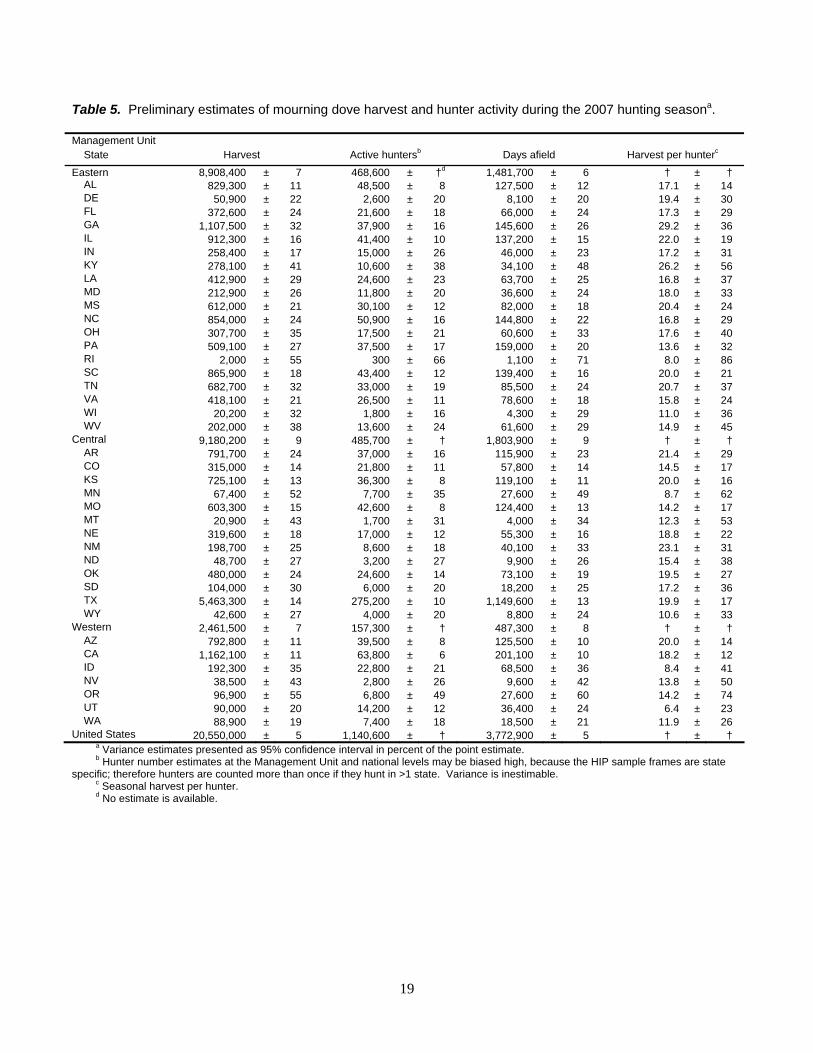
Table 5. Preliminary estimates of mourning dove harvest and hunter activity during the 2007 hunting seasona. Management Unit State Harvest Active huntersb Days afield Harvest per hunterc
Eastern 8,908,400 ± 7 468,600 ± †d 1,481,700 ± 6 † ± † AL 829,300 ± 11 48,500 ± 8 127,500 ± 12 17.1 ± 14 DE 50,900 ± 22 2,600 ± 20 8,100 ± 20 19.4 ± 30 FL 372,600 ± 24 21,600 ± 18 66,000 ± 24 17.3 ± 29 GA 1,107,500 ± 32 37,900 ± 16 145,600 ± 26 29.2 ± 36 IL 912,300 ± 16 41,400 ± 10 137,200 ± 15 22.0 ± 19 IN 258,400 ± 17 15,000 ± 26 46,000 ± 23 17.2 ± 31 KY 278,100 ± 41 10,600 ± 38 34,100 ± 48 26.2 ± 56 LA 412,900 ± 29 24,600 ± 23 63,700 ± 25 16.8 ± 37 MD 212,900 ± 26 11,800 ± 20 36,600 ± 24 18.0 ± 33 MS 612,000 ± 21 30,100 ± 12 82,000 ± 18 20.4 ± 24 NC 854,000 ± 24 50,900 ± 16 144,800 ± 22 16.8 ± 29 OH 307,700 ± 35 17,500 ± 21 60,600 ± 33 17.6 ± 40 PA 509,100 ± 27 37,500 ± 17 159,000 ± 20 13.6 ± 32 RI 2,000 ± 55 300 ± 66 1,100 ± 71 8.0 ± 86 SC 865,900 ± 18 43,400 ± 12 139,400 ± 16 20.0 ± 21 TN 682,700 ± 32 33,000 ± 19 85,500 ± 24 20.7 ± 37 VA 418,100 ± 21 26,500 ± 11 78,600 ± 18 15.8 ± 24 WI 20,200 ± 32 1,800 ± 16 4,300 ± 29 11.0 ± 36 WV 202,000 ± 38 13,600 ± 24 61,600 ± 29 14.9 ± 45 Central 9,180,200 ± 9 485,700 ± † 1,803,900 ± 9 † ± † AR 791,700 ± 24 37,000 ± 16 115,900 ± 23 21.4 ± 29 CO 315,000 ± 14 21,800 ± 11 57,800 ± 14 14.5 ± 17 KS 725,100 ± 13 36,300 ± 8 119,100 ± 11 20.0 ± 16 MN 67,400 ± 52 7,700 ± 35 27,600 ± 49 8.7 ± 62 MO 603,300 ± 15 42,600 ± 8 124,400 ± 13 14.2 ± 17 MT 20,900 ± 43 1,700 ± 31 4,000 ± 34 12.3 ± 53 NE 319,600 ± 18 17,000 ± 12 55,300 ± 16 18.8 ± 22 NM 198,700 ± 25 8,600 ± 18 40,100 ± 33 23.1 ± 31 ND 48,700 ± 27 3,200 ± 27 9,900 ± 26 15.4 ± 38 OK 480,000 ± 24 24,600 ± 14 73,100 ± 19 19.5 ± 27 SD 104,000 ± 30 6,000 ± 20 18,200 ± 25 17.2 ± 36 TX 5,463,300 ± 14 275,200 ± 10 1,149,600 ± 13 19.9 ± 17 WY 42,600 ± 27 4,000 ± 20 8,800 ± 24 10.6 ± 33 Western 2,461,500 ± 7 157,300 ± † 487,300 ± 8 † ± † AZ 792,800 ± 11 39,500 ± 8 125,500 ± 10 20.0 ± 14 CA 1,162,100 ± 11 63,800 ± 6 201,100 ± 10 18.2 ± 12 ID 192,300 ± 35 22,800 ± 21 68,500 ± 36 8.4 ± 41 NV 38,500 ± 43 2,800 ± 26 9,600 ± 42 13.8 ± 50 OR 96,900 ± 55 6,800 ± 49 27,600 ± 60 14.2 ± 74 UT 90,000 ± 20 14,200 ± 12 36,400 ± 24 6.4 ± 23 WA 88,900 ± 19 7,400 ± 18 18,500 ± 21 11.9 ± 26 United States 20,550,000 ± 5 1,140,600 ± † 3,772,900 ± 5 † ± †
a Variance estimates presented as 95% confidence interval in percent of the point estimate. b Hunter number estimates at the Management Unit and national levels may be biased high, because the HIP sample frames are state
specific; therefore hunters are counted more than once if they hunt in >1 state. Variance is inestimable. c Seasonal harvest per hunter. d No estimate is available.

20
Table 6. Preliminary estimates of mourning dove harvest and hunter activity during the 2008 hunting seasona. Management Unit State Harvest Active huntersb Days afield Harvest per hunterc
Eastern 7,671,800 ± 6 404,000 ± † 1,269,500 ± 6 †d ± † AL 877,400 ± 15 42,300 ± 9 113,500 ± 12 20.7 ± 17 DE 33,800 ± 35 2,000 ± 29 5,700 ± 34 16.7 ± 45 FL 516,500 ± 24 20,300 ± 16 94,800 ± 23 25.4 ± 29 GA 718,700 ± 22 36,100 ± 15 102,300 ± 19 19.9 ± 27 IL 683,100 ± 21 31,600 ± 12 97,000 ± 18 21.6 ± 24 IN 255,700 ± 16 14,300 ± 17 38,500 ± 17 17.9 ± 23 KY 369,400 ± 18 18,700 ± 21 43,700 ± 17 19.8 ± 28 LA 188,200 ± 38 17,200 ± 26 38,400 ± 31 11.0 ± 46 MD 151,800 ± 26 9,300 ± 19 28,400 ± 25 16.3 ± 32 MS 452,400 ± 20 17,300 ± 11 53,800 ± 18 26.1 ± 23 NC 757,900 ± 18 43,800 ± 15 112,900 ± 18 17.3 ± 24 OH 205,900 ± 28 13,500 ± 21 61,600 ± 32 15.3 ± 35 PA 340,900 ± 19 30,700 ± 19 129,900 ± 24 11.1 ± 26 RI 4,400 ± 108 300 ± 61 2,000 ± 78 13.4 ± 124 SC 844,500 ± 17 39,900 ± 12 140,900 ± 19 21.2 ± 21 TN 798,200 ± 38 37,500 ± 16 103,000 ± 30 21.3 ± 41 VA 333,600 ± 27 17,300 ± 20 59,000 ± 23 19.3 ± 33 WI 122,300 ± 37 10,500 ± 26 40,600 ± 31 11.6 ± 45 WV 16,900 ± 29 1,400 ± 20 3,700 ± 28 12.0 ± 35 Central 7,520,000 ± 10 443,900 ± † 1,496,900 ± 9 † ± † AR 422,000 ± 23 23,300 ± 18 76,600 ± 33 18.1 ± 29 CO 288,400 ± 19 23,200 ± 12 60,400 ± 18 12.4 ± 23 KS 443,700 ± 15 26,800 ± 11 78,500 ± 15 16.6 ± 19 MN 83,500 ± 48 11,300 ± 28 34,900 ± 42 7.4 ± 55 MO 467,800 ± 16 34,300 ± 9 93,400 ± 14 13.7 ± 19 MT 18,400 ± 51 2,100 ± 45 3,700 ± 44 8.8 ± 68 NE 238,600 ± 49 13,600 ± 33 48,800 ± 52 17.6 ± 59 NM 138,100 ± 30 6,300 ± 18 26,200 ± 29 22.0 ± 35 ND 26,400 ± 31 2,700 ± 30 9,200 ± 44 9.6 ± 43 OK 361,200 ± 18 19,300 ± 12 57,800 ± 17 18.7 ± 22 SD 152,100 ± 30 7,300 ± 18 27,500 ± 34 20.9 ± 35 TX 4,849,600 ± 14 271,300 ± 10 974,100 ± 13 17.9 ± 18 WY 30,100 ± 36 2,500 ± 25 5,900 ± 33 11.9 ± 44 Western 2,210,700 ± 8 146,100 ± † 426,200 ± 7 † ± † AZ 726,600 ± 12 34,000 ± 10 118,000 ± 13 21.4 ± 16 CA 1,113,700 ± 12 72,700 ± 7 207,200 ± 10 15.3 ± 14 ID 127,400 ± 24 11,800 ± 19 33,600 ± 25 10.8 ± 30 NV 45,000 ± 25 4,900 ± 15 12,200 ± 26 9.1 ± 29 OR 45,500 ± 35 5,800 ± 22 14,600 ± 28 7.9 ± 42 UT 74,100 ± 38 9,600 ± 28 22,100 ± 33 7.7 ± 48 WA 78,500 ± 31 7,300 ± 23 18,500 ± 31 10.8 ± 38 United States 17,402,400 ± 5 994,100 ± † 3,192,600 ± 5 † ± †
a Variance estimates presented as 95% confidence interval in percent of the point estimate. b Hunter number estimates at the Management Unit and national levels may be biased high, because the HIP sample frames are state
specific; therefore hunters are counted more than once if they hunt in >1 state. Variance is inestimable. c Seasonal harvest per hunter. d No estimate is available.

21
Appendix A. History of federal framework dates, season length, and daily bag limits for hunting mourning doves in the United States. Management Unit Eastern Central Western Year Datesa Days Bag Dates Days Bag Dates Days Bag 1918 Sep 1–Dec 31 107 25 Sep 1–Dec 15 106 25 Sep 1–Dec 15 106 251919–22 Sep 1–Jan 31 108 25 Sep 1–Dec 15 106 25 Sep 1–Dec 15 106 25 1923-28 Sep 1–Jan 31 108 25 Sep 1–Dec 31 106 25 Sep 1–Dec 15 106 25 1929 Sep 1–Jan 31 106 25 Sep 1–Dec 31 106 25 Sep 1–Dec 15 106 25 1930 Sep 1–Jan 31 108 25 Sep 1–Dec 15 106 25 Sep 1–Dec 15 106 25 1931 Sep 1–Jan 31 106 25 Sep 1–Dec 15 106 25 Sep 1–Dec 15 106 25 1932–33 Sep 1–Jan 31 106 18 Sep 1–Dec 15 106 18 Sep 1–Dec 15 106 18 1934 Sep 1–Jan 31 106 18 Sep 1–Jan 15 106 18 Sep 1–Dec 15 106 18 1935 Sep 1–Jan 31 107 20 Sep 1–Jan 16 106 20 Sep 1–Jan 05 107 20 1936 Sep 1–Jan 31 77 20 Sep 1–Jan 16 76 20 Sep 1–Nov 15 76 20 1937b Sep 1–Jan 31 77 15 Sep 1–Nov 15 76 15 Sep 1–Nov 15 76 15 1938 Sep 1–Jan 31 78 15 Sep 1–Nov 15 76 15 Sep 1–Nov 15 76 15 1939 Sep 1–Jan 31 78 15 Sep 1–Jan 31 77 15 Sep 1–Nov 15 76 15 1940 Sep 1–Jan 31 77 12 Sep 1–Jan 31 76 12 Sep 1–Nov 15 76 12 1941 Sep 1–Jan 31 62 12 Sep 1–Oct 27 42 12 Sep 1–Oct 12 42 12 1942 Sep 1–Oct 15 30 10 Sep 1–Oct 27 42 10 Sep 1–Oct 12 42 10 1943 Sep 1–Dec 24 30 10 Sep 1–Dec 19 42 10 Sep 1–Oct 12 42 10 1944 Sep 1–Jan 20 58 10 Sep 1–Jan 20 57 10 Sep 1–Oct 25 55 10 1945 Sep 1–Jan 31 60 10 Sep 1–Jan 31 60 10 Sep 1–Oct 30 60 10 1946 Sep 1–Jan 31 61 10 Sep 1–Jan 31 60 10 Sep 1–Oct 30 60 10 1947–48c Sep 1–Jan 31 60 10 Sep 1–Dec 3 60 10 Sep 1–Oct 30 60 10 1949 Sep 1–Jan 15 30 10 Sep 1–Nov 14 45 10 Sep 1–Oct 15 45 10 1950 Sep 1–Jan 15 30 10 Sep 1–Dec 3 45 10 Sep 1–Oct 15 45 10 1951 Sep 1–Jan 15 30 8 Sep 1- Dec 24 42 10 Sep 1–Oct 15 45 10 1952 Sep 1–Jan 10 30 8 Sep 1–Nov 6 42 10 Sep 1–Oct 12 42 10 1953 Sep 1–Jan 10 30 8 Sep 1–Nov 9 42 10 Sep 1–Oct 12 42 10 1954d Sep 1–Jan 10 40 8 Sep 1–Nov 9 40 10 Sep 1–Oct 31 40 10 1955 Sep 1–Jan 10 45 8 Sep 1–Nov 28 45 10 Sep 1–Dec 31 45 10 1956e Sep 1–Jan 10 55 8 Sep 1–Jan 10 55 10 Sep 1–Jan 10 50 10 1957 Sep 1–Jan 10 60 10 Sep 1–Jan 10 60 10 Sep 1–Jan 10 50 10 1958–59 Sep 1–Jan 15 65 10 Sep 1–Jan 15 65 10 Sep 1–Jan 15 50 10 1960–61f Sep 1–Jan 15 70g 12 Sep 1–Jan 15 60 15 Sep 1–Jan 15 50 10 1962 Sep 1–Jan 15 70g 12 Sep 1–Jan 15 60 12 Sep 1–Jan 15 50 10 1963 Sep 1–Jan 15 70g 10 Sep 1–Jan 15 60 10 Sep 1–Jan 15 50 10 1964–67 Sep 1–Jan 15 70g 12 Sep 1–Jan 15 60 12 Sep 1–Jan 15 50 12 1968 Sep 1–Jan 15 70g 12 Sep 1–Jan 15 60 12 Sep 1–Jan 15 50 10 1969–70 Sep 1–Jan 15 70g 18h Sep 1–Jan 15 60 10 Sep 1–Jan 15 50 10 1971–79 Sep 1–Jan 15 70g 12 Sep 1–Jan 15 60 10 Sep 1–Jan 15 50 10 1980 Sep 1–Jan 15 70 12 Sep 1–Jan 15i 60 10 Sep 1–Jan 15 70j 10k
1981 Sep 1–Jan 15 70 12 Sep 1–Jan 15i 45l 15l Sep 1–Jan 15 70j 10k
1982 Sep 1–Jan 15 45m 15m Sep 1–Jan 15i 45m 15m Sep 1–Jan 15 45m 15m
1983–86 Sep 1–Jan 15 60m 15m Sep 1–Jan 15i 60m 15m Sep 1–Jan 15 60m 15m
1987–07n Sep 1–Jan 15 60m 15m Sep 1–Jan 15i 60m 15m Sep 1–Jan 15 45o 10 2008 Sep 1–Jan 15 70 15 Sep 1–Jan 15i 60m 15m Sep 1–Jan 15 45o 10
a From 1918–1947, seasons for doves and other "webless" species were selected independently and the dates were the earliest opening and latest closing dates chosen. Dates were inclusive. There were different season lengths in various states with some choosing many fewer days than others. Only bag and possession limits, and season dates were specified.
b Beginning in 1937, the bag and possession limits included white-winged doves in selected states. c From 1948–1953, states permitting dove hunting were listed by waterfowl flyway. Only bag and possession limits, and season dates
were specified. d In 1954–1955, states permitting dove hunting were listed separately. Only bag and possession limits, and season dates were specified. e From 1956–1959, states permitting dove hunting were listed separately. Framework opening and closing dates for seasons (but no
maximum days for season length) were specified for the first time along with bag and possession limits. f In 1960, states were grouped by management unit for the first time. Maximum season length was specified for the first time. g Half days. h More liberal limits allowed in conjunction with an Eastern Management Unit hunting regulations experiment. i The framework extended to January 25 in Texas.

22
Appendix A. Continued.
j 50–70 days depending on state and season timing. k Arizona was allowed 12. l States had the option of a 60-day season and daily bag limit of 12. m States had the option of a 70-day season and daily bag limit of 12. n Beginning in 2002, the limits included white-winged doves in all states in the Central Management Unit. Beginning in 2006, the limits
included white-winged doves in all states in the Eastern Management Unit. o 30–45 days depending on state and season timing.

White-winged Doves Traditionally, the Service has requested that Arizona and Texas provide information about white-winged dove status in their respective states since those states conduct their own surveys with no federal involvement. In past years, we have taken those reports and summarized them orally for discussions pertaining to the regulations-setting process. In order to provide more comprehensive information, we are including a formal report from Arizona. In the future, we expect to include a report from Texas and possibly other areas as well. Texas is transitioning to a new survey methodology that includes urban areas statewide and data have not been analyzed fully.
23

24

WHITE-WINGED DOVE STATUS IN ARIZONA, 2009 MICHAEL J. RABE, Arizona Game and Fish Department, 5000 W. Carefree Highway, Phoenix, Arizona 85086-
5000, USA Abstract: The Arizona Game and Fish Department (AGFD) has monitored white-winged dove populations by means of a call-count survey to provide an annual index to population size. It runs concurrently with the U.S. Fish and Wildlife Service’s Mourning Dove Call-count Survey. The index peaked at 52.3 mean number doves heard per route in 1968, but fell precipitously in the late 1970s. The index has stabilized to around 25 doves per route in the last few years; in 2009, the mean number of doves heard per route was 27.9. AGFD also monitors harvest. Harvest during the 15-day season (September 1-15) peaked in the late 1960’s at ~740,000 birds (1968 AGFD estimate) and has since stabilized at around 100,000 birds; the preliminary 2008 Migratory Bird Harvest Information Program (HIP) estimate of harvest was 95,300 birds. In 2007, AGFD redesigned their dove harvest survey to sample only from hunters registered under HIP so that results from the AGFD survey would be comparable to those from HIP. The preliminary 2008 Arizona harvest estimate was 79,488.
BACKGROUND The white-winged dove (Zenaida asiatica) is one of 14 species of Columbidae occurring in North America north of Mexico (Aldrich 1993). Twelve subspecies of white-winged doves have been described for North, Central and South America, and the West Indies (Saunders 1968). Of these, four are known to reside and breed in the United States (Western, Z. a. mearnsi; Eastern, Z. a. asiatica; Big Bend, Z. a. grandis; and Mexican Highland, Z. a. monticola). Only the Western and Eastern races represent populations of significant size in the U.S. In Arizona, only the Western subspecies is known to occur (Fig. 1). Distribution of the white-winged dove in Arizona is mostly restricted to lower desert areas although there are infrequent reports of birds summering as far north as Flagstaff, (2,100 m elevation). The highest populations occur in the lowland Sonoran desert areas. Large numbers of birds can be found in the urban complexes of Phoenix and Tucson. There are small populations in Casa Grande and Tucson that apparently do not migrate. White-winged doves nest at relatively low densities throughout the Sonoran, Mohave, and Chihuahua deserts of southern and western Arizona, southern California, and southern New Mexico. However, in riparian woodlands near agricultural areas, populations have historically been present in high densities. Butler (1977) found that birds that nested in high densities in
mesquite (Prosopis sp) or salt cedar (Tamarix ramosissima) had higher nest success. Brown (1977) referred to these nesting concentrations as colonial
Figure. 1. The principal breeding, wintering, and resident area of migratory white-winged dove populations in North America, from George et al. (1994). Since George et al. (1994), white-winged doves have expanded their range into north-central New Mexico and southern Colorado. These new range expansions most likely are Mexican highland birds. The Eastern Population has expanded northward throughout most of the central United States.

populations, as opposed to the non-colonial populations in upland desert regions. Cottam and Trefethen (1968) speculated that white-winged doves may have been relatively uncommon in Arizona prior to the advent of agriculture because of the near absence of white-winged dove remains at prehistoric ruins in Arizona and because early European explorers failed to mention the species in their journals. Although many of the early explorations in Arizona were conducted during cool winter months after white-winged doves had presumably migrated south, some expeditions occurred during the nesting season; surely the dove’s presence would have been documented had the populations along the Gila River approached even current densities. Cottam and Trefethen (1968) present arguments that the Imperial Valley population represents a relatively recent range expansion, probably since 1901, as the result of flooding of the Salton Sink and subsequent development of agriculture. In contrast, Brown (1989:239) maintains that white-winged doves were common in Arizona from the beginning of settlement. Haughey (1986) studied desert nesting white-winged doves and their relationships to saguaro cactus (Carnegiea gigantea) in the Saguaro National Monument in southern Arizona, where they are totally dependent on native food sources. Saguaros were used extensively for both nectar and fruit in Arizona. The similarity in the nesting range of white-winged doves and that of the saguaro has been cited by several authors as noted by Haughey (1986). Those areas where white-wings occur and saguaro do not, i.e., southeastern California, southwestern New Mexico, southeastern Arizona and southern Nevada, may represent recent range extensions in response to agriculture. In recent times, white-winged dove densities have been greatest in areas near agriculture because of the abundance of food available there. Response of white-winged doves to agricultural activities are well documented and are likely partially responsible for recent large changes in abundance in the southwestern U.S. Rapid declines in white-winged dove populations following either loss of food crops or nesting habitat have been noted in Arizona (Cunningham et al. 1977, Rea 1983) and Mexico (Tomlinson 1993). White-winged doves typically migrate into Arizona beginning in March. Breeding usually occurs in two
peaks in the summer, although the timing of their breeding varies among years. The peak breeding times for these desert doves occur from May-June to July-August (Cunningham et al., 1977). Breeding in urban areas also occurs in two peaks but may be somewhat offset in timing compared to the desert birds. By early September, most of the adult birds have already begun the migration south. The young leave the state soon after. In most years much of the harvest consists of juvenile birds. IMPORTANCE White-winged doves are important pollinators of saguaro cactus in Arizona. Haughey (1986) noted that white-winged doves visited saguaro blooms more often than any other bird species. For desert-dwelling doves, 60% or more of the diet is saguaro (Haughey 1986, Wolf and Martinez del Rio 2000). Haughey (1986) suggested that the breeding cycle of these birds is timed to coincide with the saguaro bloom. Fleming et al. (1996) identified white-winged doves as the major vertebrate pollinator of saguaro. White-winged doves are also popular with non-hunting interests. People in many areas provide feeding stations and water in backyards to attract them for observation. Bird watchers and photographers also avidly pursue white-winged doves for observation and the satisfaction of adding them to their life-lists. POPULATION MONITORING AGFD has conducted their White-winged Dove Call-count Survey, similar to the Mourning Dove Call-count Survey, since 1962 (Table 1). Arizona collects data from 25–30 routes (the number varies with logistic circumstances that may prevent running some routes in some years). Typically, AGFD runs 19–22 routes in Sonoran/Mohave desert habitat, 3 routes in chaparral habitat, and 4–5 routes in Chihuahua desert habitat. The index is calculated as a simple weighted mean of the counts from the single year. In 2009, 26 routes were run: 19 in Sonoran Desert, 3 in chaparral, and 4 in Chihuahua desert habitat. The Sonoran routes were weighted 0.731 (19/26), chaparral 0.115 (3/26) and the Chihuahua desert route mean was weighed as 0.154 (4/26) of the total yearly mean. The numbers of routes in each habitat are representative of the total
26

area of white-winged dove habitat in the state. There is no attempt to monitor the population of urban doves. The index peaked at 52.3 mean doves heard per route in 1968 and decreased significantly during the next four years to less than 40 doves per route. Indices remained fairly stable from 1985-2000. Call-counts have declined since then (Table 1, Fig. 2). Most of the recent white-winged dove decline in Arizona is likely due to loss of large nesting colonies in the 1960’s and 1970’s from habitat destruction, shifts in agricultural trends, and possible over harvest. Clearing of the large mesquite forests in river bottoms for flood control and fuel wood removed the most productive nest areas. Large breeding colonies in the past were attracted to and maintained by grain fields that now grow vegetables and cotton. The more dispersed, solitary nesting white-winged populations have been less affected by these changes and have remained relatively stable in Arizona. Two check stations are run on opening day (September 1) for the dove season in Arizona. One check station is at Milligan Road, near Picacho, Arizona. The other check station is at Robbin’s Butte, a state wildlife area managed by AGFD and located west of Buckeye, Arizona. Both areas were chosen because they were popular with dove hunters and have been monitored since 1968. The number of white-winged doves examined at the two check stations varies from year to year, and numbered in the thousands in the late 1960s
and early 1970s. The number of dove hunters and doves monitored has since declined due to loss of hunters and changes in the bag limit. In a typical year, 250–500 doves are sampled to estimate the percent of young in the harvest. Since 1968 to the 2008 season, mean percent young was 62.8 (SE = 1.86, n = 41) (Table 1). HARVEST Hunting season dates and bag limits in Arizona have changed significantly during the past 60 years (Table 2; see Cottam and Trefethen 1968:320 for Arizona regulations prior to 1956), becoming much more restrictive since 1970. Arizona has conducted random mail surveys of general license holders to obtain harvest statistics specific to white-winged doves (Table 2, and Fig. 2). These surveys are sent to general license holders at the end of the season. From 1982 to 2001, the mean number of white-winged hunters per year sampled from this survey was 430. Results of the surveys are then multiplied by the estimated proportion of license holders that hunted doves each year. In 2007, AGFD redefined the sampling frame for their white-winged dove harvest survey. Instead of surveying a random sample of state hunting license holders, the survey sampled hunters who had migratory bird stamps. Thus AGFD harvest survey and HIP are now using the same sampling frame,
Y E A R
1 9 6 0 1 9 6 4 1 9 6 8 1 9 7 2 1 9 7 6 1 9 8 0 1 9 8 4 1 9 8 8 1 9 9 2 1 9 9 6 2 0 0 0 2 0 0 4 2 0 0 8
Mea
n D
oves
Hea
rd p
er R
oute
1 5
2 0
2 5
3 0
3 5
4 0
4 5
5 0
5 5
HA
RVE
ST
0
1 0 0 0 0 0
2 0 0 0 0 0
3 0 0 0 0 0
4 0 0 0 0 0
5 0 0 0 0 0
6 0 0 0 0 0
7 0 0 0 0 0
8 0 0 0 0 0
D o v e s h e a r d p e r r o u t eH a r v e s t
Figure 2. Mean white-winged doves heard per route and harvest in Arizona, 1975–2009. Harvest estimates from 2002–2008 are from the Harvest Information Program; prior to 2002, estimates are from Arizona Game and Fish Department’s small game harvest survey.
27

although the two programs make no effort to survey the same hunters. AGFD sampled 8,200 white-winged dove hunters in 2007 and 8,000 hunters in 2008. The revised AGFD harvest survey is more likely to provide results similar to HIP. In the past, AGFD estimates differed from HIP estimates, sometimes by a substantial amount (Table 3). White-winged dove populations in high-density nesting areas have been subjected to high hunting pressure, particularly during the 1960s when the bag limit in Arizona was 25 birds per day (Table 2). White-winged doves appear more vulnerable to over harvest than mourning doves (George 1993). A combination of high dove harvest in Arizona during the 1960s (Fig. 2), destruction of river-bottom nesting habitat, and a shift in agricultural crops (substantial shifts from cereal grains to cotton and other non-food crops) (Cunningham et al. 1977) was associated with declining harvests. In response, bag limits were reduced from 25 per day to 10 per day in 1970. Continued harvest declines prompted further reduction in bag limits (6 per day) in 1980 where they remain today. In 1988, season length was reduced from 3 weeks to 2 weeks and half day shooting was implemented in 1989 (Table 1). The white-winged dove harvest in Arizona peaked in 1968 (740,000) and dropped to a plateau of about 400,000 for 7 or 8 years in the mid-1970s (Table 1). However, it has continued to decline. Although the specific levels of harvest estimates are likely inaccurate, the downward trend is real. The declining harvest trend can be partially attributed to hunting restrictions, but there clearly are far fewer white-winged doves in Arizona now than there were in the 1950s and 1960s. Recent discrepancies between the call-counts and harvest trends appears to be a function of the disproportionate weight given by the call-count survey to desert nesting populations that have not experienced as much habitat loss, changes in food availability, and high hunting pressure colonial nesting doves have. Arizona white-winged dove harvest appears to have stabilized since 1/2 day shooting hours were implemented in 1989 (Tables 1 and 2). ACKNOWLEDGMENTS I thank AGFD Wildlife Managers who conducted surveys and collected data used in this report. Also, I
am grateful to D.D. Dolton (USFWS) for helping to edit and format this report while T. A. Sanders, R. D. Rau, K. Parker, and M.D. Koneff reviewed a draft and provided helpful comments. LITERATURE CITED Aldrich, J. W. 1993. Classification and distribution.
Pages 47-54 in T.S. Baskett, T. S., Sayre, M.W. Tomlinson, R.E. and R.E. Mirarchi, editors. Ecology and management of the mourning dove. Wildlife Management Institute, Washington, D.C., USA.
Brown, D. E. 1977. White-winged dove (Zenaida asiatica). Pages 217-274 in G. C. Sanderson, editor. Management of migratory shore and upland game birds in North America. International Association of Fish and Wildlife Agencies, Washington, D.C., USA.
Brown, D. E. 1989. Arizona game birds. The University of Arizona Press. Tucson, Arizona, USA.
Butler, W. I. 1977. A white-winged dove nesting study in three riparian communities on the lower Colorado River. M. S. Thesis, Arizona State University, Tempe, Arizona, USA.
Cottam C. and J. B. Trefethen. 1968. Whitewings: The Life History, Status, and Management of the White-winged Dove. D. van Nostrand Company Inc., Princeton, New Jersey, USA.
Cunningham, S. C., Engel-Wilson, R. W., Smith, P. M., and W. B. Ballard. 1977. Food habitat and nesting characteristics of sympatric mourning doves in Buckeye-Arlington Valley, Arizona. Arizona Game and Fish Department Technical Report 26, Phoenix, Arizona, USA.
Fleming, T. E., M. D. Tuttle, and M. A. Horner. 1996. Pollination biology and the relative importance of nocturnal and diurnal pollinators in three species of Sonoran desert columnar cacti. Southwestern Naturalist 41: 257-269.
George, R. R. 1993. White-winged dove banding analysis. Final Report. Federal Aid Project W-128-R, Job 6. Texas Parks and Wildlife Department, Austin Texas, USA.
George, R. R., R. E. Tomlinson, R. W. Engle-Wilson, G. L. Waggerman, A. G. Spratt. 1994. White-winged dove. Pages 29-50 in T. C. Tacha and C. E. Braun, editors. Migratory Shore and Upland Game Bird Management in North America.
28

Tomlinson, R. E. 1993. White-winged dove nesting areas in Tamaulipas, Mexico. Trip report. Office of Migratory Bird Management, US Fish and Wildlife Service, Albuquerque, New Mexico, USA.
International Association of Fish and Wildlife Agencies, Washington, D. C., USA.
Haughey, R. A. 1986. Diet of desert nesting western white-winged doves. M.S. Thesis, Arizona State University, Tempe, Arizona, USA.
Wolf, B. O. and Carlos Martinez del Rio. 2000. Use of saguaro fruit by white-winged doves: isotopic evidence of a tight ecological association. Oecologia 124:536-543.
Rea, A. M. 1983. Once a river. University of Arizona Press, Tucson, Arizona, USA.
Saunders, G. B. 1968. Seven new white-winged doves from Mexico, Central America, and southwestern United States. North American Fauna No. 65. U.S. Fish and Wildlife Service, Wash., D.C., USA.
29

Table 1. Mean number of white-winged doves heard per route and harvest from AGFD surveys, and percent young estimated in hunter bags from two check stations in Arizona, 1962–2009. Year Heard Harvest Percent young 1962 33.1 448,398 †a
1963 40.2 385,249 † 1964 35.9 412,542 † 1965 43.2 549,045 † 1966 48.4 578,166 † 1967 51.5 703,157 † 1968 52.3 740,079 57 1969 41.1 664,053 69 1970 33.9 407,921 58 1971 31.3 390,016 54 1972 35.4 355,633 79 1973 36.5 484,095 67 1974 31.0 425,127 75 1975 29.0 502,225 58 1976 30.9 455,692 66 1977 32.7 274,998 74 1978 35.6 327,555 65 1979 30.8 288,516 43 1980 34.9 75,611 51 1981 32.9 182,535 65 1982 29.3 134,981 61 1983 32.9 137,284 83 1984 31.1 177,957 82 1985 37.7 194,508 41 1986 34.1 192,734 69 1987 29.9 112,838 78 1988 26.7 99,955 78 1989 30.7 74,944 73 1990 28.0 100,163 71 1991 30.6 107,455 46 1992 30.8 94,551 63 1993 32.6 107,393 51 1994 26.9 138,080 44 1995 31.2 106,925 51 1996 31.1 140,974 63 1997 31.0 119,446 56 1998 35.0 165,190 41 1999 26.2 135,226 68 2000 30.9 123,259 70 2001 28.5 102,941 45 2002 24.6 186,532 61 2003 20.3 147,711 55 2004 20.3 86,355 69 2005 25.2 139,984 82 2006 25.0 236,126 60 2007 24.7 84,142 61 2008 26.9 79,488 74 2009 27.9 † †
a No estimate is available.
30

Table 2. White-winged dove season dates, days, and daily bag and possession limits in Arizona, 1956–2009.
Year Datesa Days Bag/possessionb
1956 Sep 1–Oct 4 and Dec 8–23 34 and 16 12/15 1957 Sep 1–29 and Dec 7–27 29 and 21 25/25 1958 Sep 1–28 and Dec 13–Jan 3 27 and 23 25/25 1960 Sep 1–25 and Dec 10–Jan 3 25 and25 25/25 1961 Sep 1–24 and Dec 9–Jan 3 24 and 26 25/25 1962 Sep 1–24 and Dec 8–Jan 2 24 and 26 25/25 1963 Sep 1–25 and Dec 7–31 25 and 25 25/25 1964 Sep 1–27 and Dec 12–Jan 3 27 and 23 25/25 1965 Sep 1–26 26 25/25 1966 Sep 1–26 25 25/25 1967 Sep 1–24 24 25/25 1968 Sep 1–24 and Dec 11–Jan 5 24 and 26 25/25 1969 Sep 1–28 and Dec 21–Jan 11 28 and 22 25/25 1970 Sep 1–20 and Dec 12–Jan 10 20 and 30 10/10 1971 Sep 1–12 12 10/10 1972 Sep 1–12 12 10/10 1973 Sep 1–23 23 10/10 1974 Sep 1–22 22 10/10 1975 Sep 1–21 21 10/10 1976 Sep 1–20 20 10/10 1977 Sep 1–25 25 10/10 1978 Sep 1–24 24 10/10 1979 Sep 1–23 23 10/10 1980c Sep 1–28 28 5/10 North and 6/12 South 1981 Sep 1–27 27 6/12 1982 Sep 1–26 26 6/12 1983 Sep 1–26 25 6/12 1984 Sep 1–23 23 6/12 1985 Sep 1–22 23 6/12 1986 Sep 1–21 22 6/12 1987 Sep 1–13 21 6/12 1988 Sep 1–11 13 6/12 1989 Sep 1–10 10 6/12 1990 Sep 1–10 10 6/12 1991 Sep 1–10 10 6/12 1992 Sep 1–10 10 6/12 1993 Sep 1–12 12 6/12 1994 Sep 1–11 11 6/12 1995 Sep 1–10 10 6/12 1996 Sep 1–10 10 6/12 1997 Sep 1–14 14 6/12 1998 Sep 1–15 15 6/12 1999 Sep 1–15 15 6/12 2000 Sep 1–15 15 6/12 2001 Sep 1–15 15 6/12 2002 Sep 1–15 15 6/12 2003 Sep 1–15 15 6/12 2004 Sep 1–15 15 6/12 2005 Sep 1–15 15 6/12 2006 Sep 1–15 15 6/12 2007 Sep 1–15 15 6/12 2008 Sep 1–15 15 6/12
a Federal white-winged dove frameworks have been set to coincide with those of mourning doves. The frameworks have allowed a white-winged dove season only during the first segment of a split mourning dove season from 1971 to present. From 1983–1986, all WMU states were permitted a mourning dove framework option (including white-wings in CA, AZ, and NV) of 60 days (45 in 1982) and 15/30 aggregate bag/possession.
b Between 1957 and 1979, mourning and white-winged doves had separate limits; since 1980, aggregate bag limits permitting either 10 or 12 doves, no more than 5 or 6 could be white-wings, have been in effect.
c Arizona was divided into a special white-winged dove zone and the remainder of the state in 1979. Hunting was permitted from noon to sunset during the first 3 days of the season in the special zone. In 1980, the state was divided into North and South zones, that latter having shooting hours of sunrise to noon. Since then season and bag limits have applied statewide.
31

Table 3. Harvest and hunter participation estimates for white-winged doves in Arizona from the Migratory Bird Harvest Information Program (HIP) and Arizona Game and Fish Department (AGFD) harvest survey, 1999–2008. Note the difference between the 2006 estimates and other years. AGFD redesigned their harvest survey in 2006. The 2006 questionnaire had a 17% return rate and results may be unreliable.
Survey and Year Harvest Active hunters Days afield HIP
1999 122,100 24,900 71,200 2000 84,500 19,600 56,400 2001 86,500 12,100 62,500 2002 120,400 22,700 72,700 2003 112,300 23,000 75,500 2004 120,300 24,200 81,200 2005 110,100 21,200 65,700 2006 107,400 18,300 56,500 2007 127,600 23,200 68,700 2008 95,300 19,800 82,400
AGFD 1999 143,129 26,689 89,709 2000 128,695 28,652 87,868 2001 102,941 21,180 77,462 2002 185,654 35,747 107,525 2003 147,711 26,598 86,120 2004 86,355 20,962 69,104 2005 139,984 29,057 98,477 2006 236,126 30,017 86,255 2007 84,142 13,852 46,203 2008 79,488 13,370 44,920
32

BAND-TAILED PIGEON POPULATION STATUS, 2009 TODD A. SANDERS, U.S. Fish and Wildlife Service, Division of Migratory Bird Management, 911 NE 11th Avenue,
Portland, OR 97232-4181, USA Abstract: This report summarizes information on the abundance and harvest of band-tailed pigeons collected annually in the western United States and British Columbia. Annual counts of Interior band-tailed pigeons seen and heard per route have not changed significantly since implementation of the Breeding Bird Survey (BBS) in 1966; however, they decreased (P <0.01) over the last 10 years by a mean of 13.4 ± 3.2% ( x ± SE). Current (2008) estimates of harvest and hunter participation were 4,700 ± 1,487 birds and 12,200 ± 2,054 hunter days afield. Composition of harvest was 18.2% hatching year birds. For Pacific Coast band-tailed pigeons, annual BBS counts of birds seen and heard per route have not changed significantly since 1966, but they have increased (P = 0.03) over the last 10 years by a mean of 5.2 ± 2.4%. According to the Pacific Coast Mineral Site Survey, annual counts of Pacific Coast band-tailed pigeons seen at each mineral site have increased (P = 0.04) since the survey was experimentally implemented in 2001 by a mean of 3.4 ± 1.6%, but counts over the last 5 years appear stable. Current (2008) estimates of harvest and hunter participation were 30,200 ± 4,931 birds and 31,300 ± 5,110 hunter days afield. Composition of harvest was 25.9% hatching year birds. Current estimates of the age-related vulnerability to harvest for these populations are unknown. Band-tailed pigeons are cooperatively managed among government wildlife agencies in the western States, British Columbia, and the U.S. Fish and Wildlife Service, and Canadian Wildlife Service. Their management is detailed in population (Interior and Pacific Coast) specific management plans (Pacific Flyway Study Committee and Central Flyway Webless Migratory Game Bird Technical Committee 2001, Pacific Flyway Study Committee 1994). Maintenance of band-tailed pigeon (Patagioenas fasciata) populations in a healthy, productive state is a primary management goal. Management activities include population assessment, harvest regulation, and habitat management. Each year, counts of band-tailed pigeons heard and seen are conducted by state, provincial, federal, and other biologist in the western United States and British Columbia to monitor band-tailed pigeon populations. The resulting information is used by wildlife administrators to set annual hunting regulations.
DISTRIBUTION AND ABUNDANCE Band-tailed pigeons are divided into six subspecies, only two of which occur north of Mexico, and each occupies a disjunct geographic distribution in western North America: Pacific Coast and U.S. Interior (Fig. 1). The coastal subspecies (P. f. monilis) breeds from extreme southeastern Alaska and western British Columbia south into Washington, Oregon, California, and extreme western Nevada, primarily west of the Cascade and Sierra Nevada ranges, into Baja California; and winters from central California into northern Baja California. Some in Mexico and southern California and the few wintering north of southern California may represent non-migratory population segments. The interior subspecies (P. f. fasciata) breeds from northern Colorado and eastcentral Utah south through Arizona, New Mexico, extreme western Texas into the Sierra Madre Occidental of Mexico; and winters from northern Mexico south to at least Michoacon. Some interchange occurs between races (Schroeder and Braun 1993). Little is known about the demographics of band-tailed pigeon populations because their habits and habitat make it impractical to locate and observe or trap an adequate sample of birds. However, in the early 1970s the total population size was approximated at 2.9–7.1 million birds in Pacific Coast region and <250,000 birds in the Interior region (estimated from harvest reports and
The primary purpose of this report is to facilitate the prompt distribution of timely information. Results are preliminary and may change with the inclusion of additional data.

Figure 1. Distribution of Pacific Coast (P. f. monilis) and Interior (P. f. fasciata) band-tailed pigeons in North America (after Braun et al. 1975). band recovery rates, Braun 1994), which demonstrates the likely sizes and disparity between the two populations. ECOLOGY Band-tailed pigeons primarily inhabit coniferous forests. They are highly mobile; individuals potentially traveling long distances (up to about 32 miles) daily to feed and drink. Their diet includes buds, flowers, and fruits of deciduous trees and shrubs, especially oak, madrone, elder, dogwood, cherry, cascara, huckleberry, and blackberry, but varies seasonally and with location. Early migrants are readily attracted to grain fields and fruit orchards dispersed below the forested hills where they nest, particularly before the onset of natural foods, which are preferred. Adults, especially in summer and particularly the Pacific Coast region, frequently visit natural springs and water bodies high in mineral salts where they drink and peck at the soil between long bouts of roosting in nearby trees. Band-tailed pigeons nest primarily in conifers, occasionally in hardwoods and shrubs, within closed-canopy conifer or mixed hardwood and conifer forest stands. Nests are loosely constructed twig platforms.
Placement is highly variable ranging 6–120 feet above ground, but is generally near the bole and in dense foliage. Adults are presumably monogamous, and most clutches have one egg, however, some nesting pairs may complete up to three nesting cycles a year in mild climates offering long nesting seasons. Both parents incubate the egg and brood the squab. Nestlings are fed curdlike crop milk formed from the inside lining of the crop of both adults. Comprehensive material on the life history of the band-tailed pigeon may be found in Keppie and Braun (2000), Braun (1994), Jarvis and Passmore (1992), and Neff (1947). MONITORING METHODS The Breeding Bird Survey The North American Breeding Bird Survey (BBS) is an all bird survey that also provides an annual index to abundance of both Interior and Pacific Coast populations of band-tailed pigeons (Sauer et al. 2007). The survey is based on thousands of routes distributed along secondary roads across the United States and Canada. Each route is 24.5 miles in length and consists of 50 stops or count locations at 0.5 mile intervals. At each stop, a 3-minute count is conducted whereby every bird seen within a 0.25 radius or heard is recorded. Surveys start one-half hour before local sunrise and take about 5 hours to complete. Data for birds heard and seen at stops are combined for BBS analyses. Mineral Site Survey The Mineral Site Survey (MSS) was developed to provide an annual index to abundance of Pacific Coast band-tailed pigeons. This survey is based on work by U.S. Geological Survey scientists who examined the effectiveness of existing survey methods in detecting long- and short-term population changes. Past monitoring efforts for the Pacific Coast population relied on the BBS, which includes all birds, and other band-tailed pigeon specific surveys in Oregon (visual counts at mineral sites in August) and Washington (audio counts along transects in June). There was no specific monitoring program in California or British Columbia. Their results suggested that counts of pigeons seen near mineral sites adopted from the Oregon protocol had the greatest power to detect short-term (3- to 5-year) trends in the data (Casazza et al 2005), but they did not determine which survey most accurately indexed population abundance. Additional research illustrated
34

impacts of rainfall on mineral site surveys (Overton et al. 2005). The MSS was developed and initiated on an experimental basis in 2001 (Casazza et al. 2003), and became operational in 2004. The survey is a coordinated effort among state and provincial wildlife agencies in California, Oregon, Washington, and British Columbia, and the U.S. Fish and Wildlife Service and Canadian Wildlife Service. The MSS involves a visual count of band-tailed pigeons at select mineral sites throughout the populations range (n = 55; 12 in California, 25 in Oregon, 14 in Washington, and 4 in British Columbia) during July from one-half hour before sunrise to noon. These counts provide an index of abundance. Unfortunately, a similar survey for Interior band-tailed pigeons is not possible because use of mineral sites is primarily limited to the Pacific Coast region (Sanders and Jarvis 2000). Harvest Information Program In past years, a compilation of non-uniform, periodic state harvest surveys have been used to obtain rough estimates of the number of band-tailed pigeon hunters and birds killed. Thus, the data were of limited use at a population range level. Those data are no longer collected by states (with the exception of possibly New Mexico). Wildlife professionals have long recognized that reliable harvest surveys are needed to estimate the magnitude of harvests and monitor the impact of hunting. Since 1952, the U.S. Fish and Wildlife Service has conducted a national harvest survey (Mail Questionnaire Survey), but it was based on a sampling frame that included waterfowl hunters and so harvest of non-waterfowl species could not be estimated reliably. To remedy this problem and challenges associated with combining state surveys, the U.S. Fish and Wildlife Service and state wildlife agencies initiated the national, Migratory Bird Harvest Information Program (HIP) in 1992. This Program was designed to enable the U.S. Fish and Wildlife Service to conduct nationwide surveys that provide reliable annual estimates of the harvest of band-tailed pigeons and other migratory game bird species. Under HIP, states provide the U.S. Fish and Wildlife Service with the names and addresses of all licensed migratory bird hunters each year, and then surveys are conducted to estimate harvest and hunter participation (total harvest, number of active hunters, days hunted, and seasonal harvest per hunter) in each state. All states
except Hawaii have participated in this Program since 1998. However, estimates of band-tailed pigeon harvest and hunter participation were not available until 1999. Parts Collection Survey The Parts Collection Survey (PCS) is a secondary component of the national harvest survey, currently HIP, which began in 1961. PCS is the primary means by which the composition (species, age, and sex) of the annual harvest is assessed. The survey randomly selects a sample of hunters registered with HIP. These persons are sent envelopes in which to return one wing from each bird harvested. All wings received annually are examined at wing bees, one in each of the four flyways, in which the wings are categorized by species, age, and sex. Band-tailed pigeons were included in PCS in 1994. MONITORING RESULTS The Breeding Bird Survey Results of BBS are presented in Tables 1–3. According to the BBS survey, there is no evidence that annual counts of Interior band-tailed pigeons seen and heard per route have changed significantly since survey implementation in 1966. However, there is evidence that these counts decreased (P <0.01) over the last 10 years by a mean of 13.4 ± 3.2% ( x ± SE) and increased (P = 0.07) over the last 5 years by a mean of 11.3 ± 4.8%. For Pacific Coast band-tailed pigeons, there is no evidence that annual counts have changed significantly since 1966 or in the past 5 years. There is evidence that counts increased (P <0.03) over the last 10 years by a mean of 5.2 ± 2.4%. Caution should be used in interpreting results, particularly for the Interior region, because sample sizes (routes) and pigeon counts per route are low, variances are high, and coverage of habitat by BBS routes is poor. Mineral Site Survey Results of MSS are presented in Tables 4–5. According to the MSS survey, there is evidence (P = 0.04) that annual counts of Pacific Coast band-tailed pigeons at each mineral site increased since the survey was experimentally implemented in 2001 by a mean of 3.4 ± 1.6%. There is no evidence that counts changed significantly over the last 5 years. Caution should be used in interpreting P-values because they are approximate based on Wald’s test. Evaluation of
35

36
confidence intervals and whether or not they include zero may be more reliable. Confidence intervals are based on bootstrap methods and may be asymmetrical. MSS and BBS show similar result over the recent five years (2004–2008) in that the confidence intervals of the estimated annual change in birds detected include 0%. MSS indicated annual counts of birds seen per mineral site did not change (P = 0.94, mean = -4.9 ± 2.6%, CI = -10.1 to 0.1) and similarly BBS indicated annual counts of birds seen and heard per route did not change (P = 0.26, mean = 4.9 ± 4.4%, CI = -3.6 to 13.5). However, there is a considerable discrepancy in the magnitude of the trend point estimate between these two surveys, and the reason for this is unknown. Harvest Information Program Results of HIP are presented in Tables 6–8 for Interior band-tailed pigeons and Tables 9–11 for Pacific Coast band-tailed pigeons. According to preliminary estimates from 2008, total harvest and hunter participation for Interior band-tailed pigeons were 4,700 ± 1,487 birds and 12,200 ± 2,054 hunter days afield. Total harvest and hunter participation for Pacific Coast band-tailed pigeons were 30,200 ± 4,931 birds and 31,300 ± 5,110 hunter days afield. The season was closed in Washington from 1991 through 2001. Parts Collection Survey Results of PCS are presented in Tables 12 and 13. Data from 2008 show that the composition of the Interior band-tailed pigeon harvest was comprised of 18.2% hatching year birds based on a total sample of 11 birds. Composition of the Pacific Coast band-tailed pigeon harvest was comprised of 25.9% hatching year birds based on a total sample of 270 birds. The season was closed in Washington from 1991 through 2001. Caution should be used in interpreting state specific estimates with small sample size. Also, numbers are an index to recruitment and not adjusted for differential vulnerability to harvest between age classes. Consequently, the annual composition of harvest may not be representative of the population. There is not adequate data to evaluate current differential vulnerability rates between young and adult birds (young:adult). There is however some data for male and females combined during 1968–1976 for the Interior population and during 1962–1977 for the Pacific Coast population. Estimates of young per adult bird in the
harvest are variable among years and range from 0.20 ± 0.20 to 5.62 ± 5.92 with a mean of 1.90 ± 0.60 for the Interior population and 0.55 ± 0.24 to 1.54 ± 0.81 with a mean of 1.05 ± 0.10 for the Pacific Coast population (T. A. Sanders, U.S. Fish and Wildlife Service, unpublished data). These results suggest that on average young are nearly twice as likely to be harvested compared to adults in the Interior population, whereas young and adult birds alike have nearly equal probability of harvest in the Pacific Coast population. The difference in age-related vulnerability between the populations may be related to the use of mineral sites by the Pacific Coast population and associated exposure to harvest. It is unknown whether these mean age-related vulnerability estimates apply to more recent years. But if they do, then the proportion of young in the Interior population may be about half of that estimated from PCS, whereas the proportion of young in the Pacific Coast population may be as estimated from PCS. ACKNOWLEDGMENTS Personnel of state wildlife agencies and the U.S. Fish and Wildlife Service (USFWS) cooperated in collecting the data presented in this report. Special thanks to J. Garcia (CA), B. Reishus (OR), D. Kraege (WA), and Andrea Breault (BC) for their role in coordination of the MSS and providing data. J. R. Sauer (USGS) analyzed BBS data and provided statistical support. K. Richkus (USFWS) provided the HIP and PCS data. M. Koneff (USFWS), D. Dolton (USFWS), Rebecca Rau (USFWS), and Keri Parker (USFWS) reviewed a draft of this report. LITERATURE CITED Braun, C. E. 1994. Band-tailed Pigeon. Pages 60–74 in
T. C. Tacha and C. E. Braun, editors. Migratory shore and upland game bird management in North America. International Association of Fish and Wildlife Agencies, Washington, D.C.
Braun, C. E., D. E. Brown, J. C. Pederson, and T. P. Zapatka. 1975. Results of the Four Corners cooperative band-tailed pigeon investigation. U.S. Fish and Wildlife Service, Resource Publication 126.
Casazza, M. L., C. T. Overton, J. L. Yee, D. L. Orthmeyer, M. R. Miller, and R. A. Schmitz. 2003. Development of a reliable population index for Pacific Coast band-tailed pigeons: final report. U.S. Geological Survey, Western Ecological Research

37
Center, Dixon Field Station, Dixon, CA. Unpublished report.
Casazza, M. L., J. L. Yee, M. R. Miller, D. L. Orthmeyer, D. R. Yparraguirre, R. L. Jarvis, and C. T. Overton. 2005. Evaluation of current population indices for band-tailed pigeons. Wildlife Society Bulletin 33(2):606–615.
Jarvis, R. L., and M. F. Passmore. 1992. Ecology of band-tailed pigeons in Oregon. U.S. Fish and Wildlife Service, Biological Report 6.
Keppie, D. M., and C. E. Braun. 2000. Band-tailed pigeon (Columbia fasciata). In A. Poole and F. Gill, editors. The Birds of North America, No. 530. The Birds of North America, Inc., Philidelphia, PA.
Neff, J. A. 1947. Habits, food, and economic status of the band-tailed pigeon. U.S. Fish and Wildlife Service, North American Fauna Number 58.
Overton, C. T., R. A. Schmitz, and M. L. Casazza. 2005. Post-precipitation bias in band-tailed pigeon surveys conducted at mineral sites. Wildlife Society Bulletin 33(3):1047–1054.
Pacific Flyway Study Committee and Central Flyway Webless Migratory Game Bird Technical Committee. 2001. Pacific and Central Flyways management plan for the Four Corners population of band-tailed pigeons. Pacific Flyway Council, c/o U.S. Fish and Wildlife Service, Portland, Oregon.
Pacific Flyway Study Committee. 1994. Pacific Flyway management plan for the Pacific coast population of band-tailed pigeons. Pacific Flyway Council, c/o U.S. Fish and Wildlife Service, Portland, Oregon.
Sanders, T. A., and R. L. Jarvis. 2000. Do band-tailed pigeons seek a calcium supplement at mineral sites? Condor 102:855–863.
Sauer, J. R., J. E. Hines, and J. Fallon. 2007. The North American Breeding Bird Survey, Results and Analysis 1966–2006. Version 10.13.2007. USGS Patuxent Wildlife Research Center, Laurel, MD.
Schroeder, M. A., and C. E. Braun. 1993. Movement and philopatry of band-tailed pigeons captured in Colorado. Journal of Wildlife Management 57:103–112.

Table 1. Breeding Bird Survey 43-year (1966–2008) trend estimates (expressed as mean annual percentage change in abundance) and 95% confidence intervals for band-tailed pigeons seen and heard along routes. Trend Mean Region x SE LCI UCI P-value per route Routes Interiora -2.9 2.2 -7.2 1.4 0.20 0.6 34 Arizona -1.3 7.3 -15.6 13.0 0.86 0.8 12 Colorado 10.2 6.4 -2.3 22.6 0.14 0.1 12 New Mexico -8.6 1.6 -11.8 -5.4 <0.01 1.0 9 Pacific Coast -0.7 1.0 -2.6 1.2 0.46 2.6 198 British Columbia -2.1 2.8 -7.6 3.3 0.45 1.6 28 California -0.1 1.4 -2.8 2.6 0.95 2.2 108 Oregon -0.4 1.0 -2.3 1.5 0.67 4.1 33 Washington 0.6 1.2 -1.6 2.9 0.60 4.0 29
a No estimates for Utah are available. Table 2. Breeding Bird Survey 10-year (1999–2008) trend estimates (expressed as mean annual percentage change in abundance) and 95% confidence intervals for band-tailed pigeons seen and heard along routes. Trend Region x SE LCI UCI P-value Routes Interiora -13.4 3.2 -19.6 -7.2 <0.01 20 Arizona -8.9 12.5 -33.4 15.6 0.51 6 Colorado 3.1 6.2 -9.0 15.2 0.64 5 New Mexico -11.1 3.2 -17.3 -4.9 0.01 9 Pacific Coast 5.2 2.4 0.5 9.9 0.03 137 British Columbia 11.2 7.6 -3.6 26.0 0.16 16 California 6.1 1.8 2.5 9.6 0.00 75 Oregon 4.2 4.2 -4.1 12.4 0.33 25 Washington -1.2 6.4 -13.7 11.2 0.85 21
a No estimates for Utah are available. Table 3. Breeding Bird Survey 5-year (2004–2008) trend estimates (expressed as mean annual percentage change in abundance) and 95% confidence intervals for band-tailed pigeons seen and heard along routes. Trend Region x SE LCI UCI P-value Routes Interiora 11.3 4.8 1.9 20.6 0.07 10 Arizona 9.6 20.5 -30.7 49.8 0.67 4 New Mexico 30.3 9.3 12.2 48.5 0.05 6 Pacific Coast 4.9 4.4 -3.6 13.5 0.26 95 British Columbia 3.2 31.8 -59.2 65.6 0.92 7 California 1.9 3.1 -4.2 7.9 0.55 53 Oregon -0.7 10.6 -21.6 20.2 0.95 19 Washington 21.1 14.2 -6.7 48.9 0.16 16
a No estimates for Colorado or Utah are available.
38

Table 4. Mineral Site Survey 8-year (2001–2008) trend estimates (expressed as a mean annual percentage change in abundance) and 95% confidence intervals for band-tailed pigeons seen at mineral sites. Trend Mean Region x SEa LCI UCI P-valueb per site Sites Pacific Coast 3.4 1.6 0.3 6.7 0.04 180.8 55 British Columbia 8.2 5.4 1.1 19.5 0.13 118.2 4 California 4.2 5.7 -8.0 14.1 0.46 64.6 12 Oregon 4.5 2.4 0.7 10.1 0.06 243.9 25 Washington 1.0 2.4 -4.1 5.5 0.68 183.3 14
a Variance estimates are based on bootstrap simulation. b P-values are approximate based on Wald’s test.
Table 5. Mineral Site Survey 5-year (2004–2008) trend estimates (expressed as a mean annual percentage change in abundance) and 95% confidence intervals for band-tailed pigeons seen at mineral sites. Trend Mean Region x SEa LCI UCI P-valueb per site Sites Pacific Coast -4.9 2.6 -10.1 0.1 0.94 160.7 53 British Columbia -17.0 6.9 -26.8 -0.5 0.99 137.1 4 California 8.1 7.4 -5.2 22.8 0.28 80.2 12 Oregon -5.6 4.1 -13.0 3.2 0.83 192.0 23 Washington -6.6 3.5 -14.4 -0.7 0.94 184.2 14
a Variance estimates are based on bootstrap simulation. b P-values are approximate based on Wald’s test.
Table 6. Harvest Information Program harvest estimates (mean and 95% confidence interval ½ width expressed as percent of the mean) for Interior band-tailed pigeons, 1999–2008. Arizona Colorado New Mexico Utah Total Year x CI x CI x CI x CI x CI 1999 500 154 700 129 0 0 100 69 1,300 94 2000 2,300 110 1,700 147 400 122 300 192 4,600 78 2001 400 118 600 94 600 126 300 169 2,000 62 2002 1,000 153 100 117 600 158 400 149 2,100 89 2003 1,400 126 900 97 400 65 100 132 2,900 70 2004 1,400 120 500 57 700 115 200 136 2,800 68 2005 2,200 105 100 113 300 106 100 193 2,700 86 2006 500 56 600 76 100 109 400 95 1,600 42 2007 1,000 101 900 102 2,800 113 200 195 4,800 71 2008 1,600 122 2,500 83 600 95 †a † 4,700 62
B No estimate is available.
39

Table 7. Harvest Information Program active hunter estimates (mean and 95% confidence interval ½ width expressed as percent of the mean) for Interior band-tailed pigeons, 1999–2008. Arizona Colorado New Mexico Utah Totala
Year x CI x CI x CI x CI x CI 1999 700 105 100 113 100 121 <50 46 900 †b
2000 600 79 400 95 300 67 <50 192 1,300 † 2001 500 65 500 61 500 53 200 97 1,800 † 2002 400 85 200 101 300 81 200 98 1,000 † 2003 1,500 61 400 71 400 67 300 81 † † 2004 900 56 300 29 100 103 50 92 † † 2005 800 69 200 46 100 109 100 134 † † 2006 600 73 900 52 100 172 200 92 † † 2007 2,100 43 1,400 45 800 47 300 86 4,600 † 2008 1,300 55 2,300 40 600 52 300 143 4,500 †
a Estimates in total may be biased high because the HIP sample frames are state-specific; therefore, hunters are counted multiple times if they hunt in more than one state.
b No estimate is available. Table 8. Harvest Information Program days afield estimates (mean and 95% confidence interval ½ width expressed as percent of the mean) for Interior band-tailed pigeons, 1999–2008. Arizona Colorado New Mexico Utah Total Year x CI x CI x CI x CI x CI 1999 2,000 97 300 122 300 158 100 50 2,700 76 2000 1,600 83 2,800 107 900 75 300 192 5,600 60 2001 1,000 71 800 54 1,800 64 700 133 4,300 39 2002 1,000 110 400 105 900 109 500 104 2,800 58 2003 3,700 77 2,100 89 1,400 75 600 136 7,900 47 2004 2,300 80 700 35 300 92 100 72 3,400 55 2005 1,600 74 300 51 400 140 200 142 2,500 54 2006 1,100 70 1,700 63 300 163 200 87 3,300 43 2007 5,000 57 3,800 56 3,600 62 400 73 12,800 33 2008 3,300 66 6,100 45 2,100 76 700 139 12,200 33 Table 9. Harvest Information Program harvest estimates (mean and 95% confidence interval ½ width expressed as percent of the mean) for Pacific Coast band-tailed pigeons, 1999–2008. California Oregon Washington Total Year x CI x CI x CI x CI 1999 19,300 101 3,800 42 †a † 23,100 85 2000 12,200 65 4,100 92 † † 16,300 54 2001 8,300 49 5,000 45 † † 13,200 35 2002 4,200 39 4,000 36 † † 8,200 27 2003 8,000 50 4,900 33 1,500 78 14,400 31 2004 14,300 45 3,300 44 300 160 17,900 37 2005 11,100 58 1,400 34 1,000 84 13,500 48 2006 12,500 40 1,500 25 900 97 14,900 34 2007 9,700 39 1,400 74 1,700 61 12,700 32 2008 27,500 35 500 18 2,100 87 30,200 32
a The season in Washington was closed from 1991 through 2001, no estimate is available.
40

Table 10. Harvest Information Program active hunter estimates (mean and 95% confidence interval ½ width expressed as percent of the mean) for Pacific Coast band-tailed pigeons, 1999–2008. California Oregon Washington Totala
Year x CI x CI x CI x CI 1999 3,900 48 1,500 47 †b † 5,400 † 2000 5,600 37 1,700 46 † † 7,300 † 2001 2,600 34 1,700 31 † † 4,200 † 2002 2,500 30 1,300 25 † † 3,800 † 2003 4,600 38 1,800 24 1,000 23 † † 2004 4,700 37 1,500 36 500 64 † † 2005 3,900 39 500 14 700 58 † † 2006 6,000 35 400 13 500 61 † † 2007 4,900 33 700 113 900 44 6,500 † 2008 10,500 24 200 8 600 61 11,300 †
a Estimates in total may be biased high because the HIP sample frames are state-specific; therefore, hunters are counted multiple times if they hunt in more than one state.
b The season in Washington was closed from 1991 through 2001, no estimate is available. Table 11. Harvest Information Program days afield estimates (mean and 95% confidence interval ½ width expressed as percent of the mean) for Pacific Coast band-tailed pigeons, 1999–2008. California Oregon Washington Total Year x CI x CI x CI x CI 1999 9,100 54 3,500 33 †a † 12,600 40 2000 10,000 41 3,800 61 † † 13,800 34 2001 7,500 39 4,700 39 † † 12,200 28 2002 4,600 35 3,400 28 † † 7,900 23 2003 11,500 52 5,100 29 1,600 58 18,300 34 2004 9,700 36 3,400 35 800 83 13,900 27 2005 8,800 47 1,300 21 1,000 62 11,000 38 2006 13,500 47 1,200 20 700 68 15,400 41 2007 10,600 37 1,200 69 1,800 60 13,500 30 2008 29,300 34 500 13 1,500 70 31,300 32
a The season in Washington was closed from 1991 through 2001, no estimate is available. Table 12. Parts Collection Survey age structure of Interior band-tailed pigeons determined from hunter shot birds during September, 1994 to 2008. Values are percentage of hatch year birds (%), number of hatch year birds (n), and number of both hatch year and after hatch year birds examined (N). Arizona Colorado New Mexico Utah Total Year % n N % n N % n N % n N % n N 1994 24.6 16 65 66.7 4 6 28.6 14 49 †a 0 0 28.3 34 120 1995 60.0 6 10 28.9 52 180 19.0 12 63 54.5 6 11 28.8 76 264 1996 0.0 0 1 38.5 5 13 34.1 15 44 † 0 0 34.5 20 58 1997 33.3 7 21 31.5 17 54 15.5 13 84 † 0 0 23.3 37 159 1998 48.4 15 31 20.0 2 10 10.0 2 20 16.7 1 6 29.9 20 67 1999 13.0 3 23 33.3 6 18 24.1 7 29 † 0 0 22.9 16 70 2000 41.7 30 72 11.8 2 17 26.9 18 67 0.0 0 3 31.4 50 159 2001 52.9 9 17 † 0 0 23.5 4 17 33.3 1 3 37.8 14 37 2002 53.9 55 102 27.3 3 11 50.8 32 63 8.3 1 12 48.4 91 188 2003 † 0 0 † 0 0 33.3 1 3 † 0 0 33.3 1 3 2004 34.8 8 23 † 0 0 40.0 4 10 † 0 0 36.4 12 33 2005 15.4 2 13 66.7 8 12 0.0 0 3 † 0 0 35.7 10 28 2006 11.5 6 52 20.0 4 20 29.9 20 67 † 0 0 21.6 30 139 2007 20.5 9 44 † 0 0 † 0 0 † 0 0 20.5 4 44 2008 18.2 2 11 † 0 0 † 0 0 † 0 0 18.2 2 11
B No estimate is available.
41

42
Table 13. Parts Collection Survey age structure of Pacific Coast band-tailed pigeons determined from hunter shot birds during September through December, 1994 to 2008. Values are percentage of hatch year birds (%), number of hatch year birds (n), and number of both hatch year and after hatch year birds examined (N). California Oregon Washington Total Year % n N % n N % n N % n N 1994 44.6 226 507 22.9 131 571 †a 0 0 33.1 357 1078 1995 29.6 74 250 20.1 109 542 † 0 0 23.1 183 792 1996 27.9 68 244 15.1 38 252 † 0 0 21.4 106 496 1997 31.1 65 209 17.7 64 361 † 0 0 22.6 129 570 1998 32.0 81 253 18.4 45 244 † 0 0 25.4 126 497 1999 33.2 119 358 20.1 79 394 † 0 0 26.3 198 752 2000 32.1 69 215 17.5 58 332 † 0 0 23.2 127 547 2001 22.9 33 144 17.0 46 271 † 0 0 19.0 79 415 2002 31.5 52 165 14.1 33 234 3.8 22 180 18.5 107 579 2003 34.4 72 209 21.2 49 231 3.1 17 112 25.0 138 552 2004 25.2 33 131 19.6 38 194 2.6 9 27 22.7 80 352 2005 18.8 25 133 13.3 24 180 † 0 0 15.7 49 313 2006 18.1 47 260 19.0 48 253 13.6 6 44 18.1 101 557 2007 24.8 34 137 14.3 36 251 10.9 6 55 17.2 76 443 2008 29.8 39 131 20.0 22 110 31.0 9 29 25.9 70 270
a The season in Washington was closed from 1991 through 2001, no estimate is available.

U.S. Fish and Wildlife ServiceDivision of Migratory Bird ManagementPopulation and Habitat Assessment Branch11510 American Holly DriveLaurel, Maryland, 20708-4016
http://www.fws.gov
June 2009
For State Transfer Relay Services: TTY/Voice: 711