US building energy efficiency and flexibility as an ...

llOPEN ACCESS

Article

US building energy efficiency and flexibility asan electric grid resource

Jared Langevin, Chioke B.

Harris, Aven Satre-Meloy, Handi

Chandra-Putra, Andrew Speake,

Elaina Present, Rajendra

Adhikari, Eric J.H. Wilson,

Andrew J. Satchwell

[email protected]

Highlights

The technical potential US

building-grid resource is

quantified for 2030 and 2050

Co-deployment of building

efficiency and flexibility yields the

largest load impacts

Up to 800 TWh generation and

208 GW daily net peak demand

could be avoided

Preconditioning and plug load

management are among the most

impactful measures

Buildings consume 75% of US electricity and could be a primary demand-side

management resource for the rapidly changing electric grid. We assess the

technical potential grid resource from best-available building efficiency and

flexibility measures in 2030 and 2050 and find that such measures could avoid up

to nearly one-third of annual fossil-fired generation and one-half of fossil-fired

capacity additions after 2020. Our results quantify the role that building

technologies can play in the future of the US electricity system.

Langevin et al., Joule 5, 1–27

August 18, 2021 ª 2021 The Authors. Published

by Elsevier Inc.

https://doi.org/10.1016/j.joule.2021.06.002

mailto:[email protected]


llOPEN ACCESS

Please cite this article in press as: Langevin et al., US building energy efficiency and flexibility as an electric grid resource, Joule (2021), https://doi.org/10.1016/j.joule.2021.06.002

Article

US building energy efficiencyand flexibility as an electric grid resource

Jared Langevin,1,4,* Chioke B. Harris,2 Aven Satre-Meloy,1 Handi Chandra-Putra,1 Andrew Speake,2

Elaina Present,2 Rajendra Adhikari,2 Eric J.H. Wilson,2 and Andrew J. Satchwell3

Context & scale

The US electricity system is

undergoing a rapid

transformation, with renewable

generation sources projected to

account for the majority of annual

electricity generation as soon as

2035. While policymakers have

focused on power sector

decarbonization as a critical

component of net zero

greenhouse gas emissions

pathways, emerging evidence

underscores the role of demand-

side technologies in facilitating a

decarbonized energy system.

Using a reproducible modeling

SUMMARY

Buildings use 75% of US electricity; therefore, improving the effi-ciency and flexibility of building operations could provide significantvalue to the rapidly changing electricity system. Here, we estimatethe technical potential near- and long-term impacts of best-avail-able building efficiency and flexibility measures on annual electricityuse and hourly demand across the contiguous United States. Co-deployment of building efficiency and flexibility avoids up to 742TWh of annual electricity use and 181 GW of daily net peak load in2030, rising to 800 TWh and 208 GW by 2050; at least 59 GW and69 GW of the peak reductions are dispatchable. Implementing effi-ciency measures alongside flexibility measures reduces the poten-tial for off-peak load increases, underscoring limitations on loadshifting in efficient buildings. Overall, however, we find a substantialbuilding-grid resource that could reduce future fossil-fired genera-tion needs while also reducing dependence on energy storagewith increasing variable renewable energy penetration.

framework, we quantify the grid

resource from building efficiency

and flexibility at the national scale,

demonstrate how this resource

varies across grid regions and

hours of the day, and identify

specific building technologies

that drive grid-scale impacts. The

capabilities and results that we

report can improve the

representation of demand-

management strategies in policy

development and grid planning

that seeks to reduce future US

fossil-fired generation needs and

enable increased variable

renewable-energy supply.

INTRODUCTION

The US electricity system is undergoing a rapid transformation. Non-hydro renew-

able energy deployment reached a record 80% of new US electric-generating capac-

ity in 2020 and has accounted for 60% of total capacity additions in the last decade.1

Recent projections estimate that these sources will account for the largest share of

electricity generation as early as 2035.2,3 Researchers and policymakers have

focused on power-sector decarbonization as a critical component of net zero green-

house gas emissions pathways; however, an emerging body of evidence suggests

that parallel demand-side solutions are also important for achieving ambitious

climate change mitigation targets.4–6 Creutzig et al.4 advocate for research that im-

proves the understanding of demand-side solutions in climate change mitigation

research, quantifies the impact potentials for specific demand-side technologies,

and assesses interactions between demand-side solutions and the energy supply

system.

Energy efficiency is a key type of demand-side solution that has been included in

past decarbonization studies and featured in recent research efforts, such as that

of Wilson et al.7 A large body of research supports the notion that energy efficiency

is one of the fastest and most broadly beneficial options for mitigating climate

change.8 More recently, energy flexibility,9 which the International Energy Agency

(IEA) defines as ‘‘the ability [for a building] to manage its demand and generation ac-

cording to local climate conditions, user needs, and grid requirements,’’10 has

emerged as a complementary demand-side solution that can reduce the costs and

Joule 5, 1–27, August 18, 2021 ª 2021 The Authors. Published by Elsevier Inc.This is an open access article under the CC BY license (http://creativecommons.org/licenses/by/4.0/).

1

http://creativecommons.org/licenses/by/4.0/

1Building Technology and Urban SystemsDivision, Lawrence Berkeley National Laboratory,Berkeley, CA 94720, USA

2Building Technologies and Science Center,National Renewable Energy Laboratory, Golden,CO 80401, USA

3Electricity Markets and Policy Department,Lawrence Berkeley National Laboratory,Berkeley, CA 94720, USA

4Lead contact

*Correspondence: [email protected]


llOPEN ACCESS


Article

ensure the reliability of power systems with high levels of renewable energy penetra-

tion. Existing literature identifies and assesses the technologies and market mecha-

nisms that can provide enhanced system flexibility,11,12 estimates the value of

flexibility to the grid,13,14 and characterizes technology pathways that support

high penetrations of renewable electricity generation,15,16 among other topics. As

the US continues to rapidly transform its electricity supply, assessing the potential

for energy efficiency and flexibility measures to support this transition is a pressing

research objective.

Improved demand management through energy efficiency and flexibility offers

several benefits to the electric grid, including: reduced power generation capacity,

operation, and maintenance costs17–19; provision of ancillary services and standing

reserves for system balancing and reliability with lower costs and emissions17,20,21;

and avoided capital costs for transmission and distribution equipment upgrades

and voltage control.17,22 Demand management technologies can be deployed

alongside energy storage to meet grid flexibility needs in a highly renewable elec-

tricity future.16 The recent US Federal Energy Regulatory Commission (FERC) Order

2222 enables aggregators of energy efficiency and demand response to participate

in wholesale electricity markets alongside traditional generation resources, acknowl-

edging the important role of demand management technologies in future electricity

systems.23

In the United States, the buildings sector accounts for 75% of electricity use24 and is

therefore a primary demand management resource for the electric grid. Building

technologies, such as highly efficient heating and cooling equipment, highly insu-

lating windows, solid-state lighting, and variable speed motors, offer substantial ef-

ficiency gains, while connected appliances and smart controls enable buildings to

actively manage electric loads to provide flexibility services to the grid while still

meeting occupant comfort and productivity requirements.25 Previous studies of

the US building-grid resource at the national scale suggest that such building tech-

nologies can reduce at least 150–200 GW of summer peak load by 2030. For

example, a landmark FERC assessment found that 2019 peak load in the US could

be reduced by 150 GW using demand response (DR) measures,26 and a comprehen-

sive bottom-up analysis from the Electric Power Research Institute (EPRI) estimated a

technical potential summer peak reduction of 304 GW from energy efficiency and

175 GW from DR by 2030.27 A more recent Brattle study estimates nearly 200 GW

of cost-effective load flexibility potential by 2030,28 while another recent national

study finds up to 40 GW of flexible reduction potential from commercial building

HVAC loads alone.29 Regional studies lend further support to these findings, and

we use results from these studies to benchmark our own findings in the discussion

section of this paper. Outside the US context, several international studies qualita-

tively describe demand management opportunities30–33 or quantitatively demon-

strate a large grid resource from building efficiency and flexibility portfolios,34–36

though the differences between US and international electricity systems and build-

ings sectors preclude a direct comparison of results.

The existing US literature establishes that buildings can play an important role in po-

wer-sector decarbonization and in limiting future growth in electricity demand. To

the authors’ knowledge, however, no existing study quantifies the magnitude of

the US building-grid resource at the national scale while also communicating its

regional and temporal variability and identifying the specific building end uses

and technologies that drive grid-scale impacts. Building technologies are highly het-

erogeneous, and few existing studies attempt to aggregate load impacts across

2 Joule 5, 1–27, August 18, 2021



llOPEN ACCESS


Article

multiple technology types to enable benchmarking against single-technology alter-

natives such as traditional power generation plants or battery storage. Moreover,

studies that do aggregate across technologies tend to focus on maximum peak

load impacts,26–28 despite the need to account for the growing influence of variable

renewable generation on daily system needs, and these studies rarely consider inter-

actions between efficiency and flexibility measures when both are included (for

example, total peak reduction from the adoption of more efficient and more flexible

HVAC is not necessarily equal to the sum of these measures’ individual peak reduc-

tions). Other key limitations of existing literature include the reliance on data sets

that are outdated and/or spatiotemporally constrained, as well as the absence of

a common and reproducible framework that can be updated to reflect continued

changes in the energy sector.

In this paper, we conduct a comprehensive analysis of the near- and long-term tech-

nical potential bulk power grid resource offered by best-available US building

efficiency and flexibility measures. Using multiple openly available modeling frame-

works, we pair bottom-up simulations of measures’ building-level impacts with

regional representations of the building stock and its projected electricity use to es-

timate the impacts of multiple building efficiency and flexibility scenarios on hourly

regional system loads across the contiguous United States in 2030 and 2050. Results

are communicated at both the national and regional scales and are disaggregated

by building type and end use, facilitating a quantitative understanding of the role

that buildings as a whole and specific building technologies or operational ap-

proaches can play in the future evolution of the US electricity system.

Building efficiency and flexibility scenarios and grid metrics

Table 1 provides an overview of the main components of the analysis framework,

supporting data sources, and key implications of the analysis design. We estimate

the technical potential impacts of three building measure sets—energy efficiency

only (EE), demand flexibility only (DF), and packaged efficiency and flexibility

(EE+DF)—on annual US residential and commercial building electricity use and

hourly electricity demand. We model the measures that make up these measure

sets using EnergyPlus; building energy modeling enables an investigation of mea-

sure impacts across the full US building stock, which is not possible with currently

available metered building electricity use data. Measure impacts in 2030 and 2050

are assessed within each of the 22 2019 US Energy Information Administration

(EIA) Electricity Market Module (EMM) regions, with certain outputs aggregated

into the 10 2019 US Environmental Protection Agency (EPA) AVoided Emissions

and geneRation Tool (AVERT) regions for simplicity of presentation (Figure 1). We

design measures and assess their impacts using a framework that seeks to approx-

imate typical daily power system conditions and operation based on economic

dispatch.37 Specifically, we use the net load shape for each region—the total hourly

load less hourly variable renewable electricity generation—as a proxy for marginal

electricity costs, and we configure flexibility measures to reduce demand during

high net load and high marginal cost hours and shift loads into low net load and

low marginal cost hours where possible. This framing better reflects the influence

of low marginal cost variable renewable generation on grid scheduling objectives

and the associated value of grid services. Renewable electricity penetration levels

vary on a regional basis, but average to 29% nationally. We focus on average daily

non-coincident net peak and off-peak hour impacts across the summer (June–

September), winter (December–March), and intermediate (all other months) sea-

sons. Non-coincident net peak is defined as the sum of individual maximum net

demands across regions regardless of the times at which they occur.38 Additional

Joule 5, 1–27, August 18, 2021 3

Table 1. Overview of primary analysis components, sources, and high-level implications of the modeling framework and approach

Component Source or definition Description Implications

Inputs

baseline buildingenergy use (demand)scenario

2019 EIA AEO39 annual building energy use projected 2015–2050 based onbusiness-as-usual (BAU) assumptions about technologyadvancement and adoption

building load electrification beyond BAU could influence loadshapes and total annual electricity use; high electrificationimplications are explored in section S1.3

baseline electricitygeneration (supply)scenario

2019 EIA AEO39 net load defined by hourly system loads less wind and solargeneration at 29% penetration of total annual generation

use of net load reflects the influence of low marginal costrenewable generation on grid scheduling objectives and theassociated value of grid services; sensitivity to higherrenewable penetrations is explored in section S2.1.1

baseline end-use loadshapes

EnergyPlus models representative end-use load shapes from EnergyPlus are usedto translate baseline electricity use to an hourly basis (seesection S2.2)

modeled end-use loads might not fully reflect the diversity ofusage patterns, which could result in both under- andoverestimation of potential from efficiency and flexibilitymeasures, depending on the building type

alternative buildingdemand scenarios––

best energy efficiencyonly (EE)

best available efficiency levels correspond to those defined byEIA or market surveys where EIA data are not available

electricity use reductions from best available technologiesrelative to the baseline might be reduced in 2050 as thebaseline improves and further efficiency gains become elusive

best demand flexibilityonly (DF)

best available flexibility levels maximize intended reductions orincreases in hourly electricity demand without compromisingminimum building service levels

flexible end-use operation designed to shift load away fromhighest net system load hours and into the lowest net systemload hours, which will reduce peak and avoid renewableenergy curtailments, but might not yield the highest possibleelectricity market value or value to an individual utility

best energy efficiencyand demand flexibility(EE+DF)

combines EE scenario end-use efficiencies with DF scenarioflexibility specifications

–

Modelcharacteristics

energy demandsegments

US residential andcommercial buildings

three residential and eleven commercial building types, withbuilding-level hourly load shapes represented by sampledresidential housing units and five commercial prototypeEnergyPlus models

EnergyPlus building types represent the majority of USbuildings but do not capture all possible variations in stockcharacteristics and resulting end-use load shapes

technology stockdynamics

technical potentialtechnology diffusion

technical potential technology adoption equates to 100%annual stock turnover, which ensures complete adoption ofmeasures in the building demand scenarios considered

from adoption alone, results represent an upper bound ofenergy savings and load shed and shift

geographic extentand resolution

contiguous US, 222019 EIA EMMregions or 10 2019EPA AVERT regions

EMM regions approximate independent system operator andNorth American Electric Reliability Corporation (NERC)assessment region boundaries; EPA AVERT regions are usedfor results aggregation for simplicity (see Figure 1)

focus is on regional and national-level impacts; building-,campus-, or feeder-level focus might yield different results

temporal extent andresolution

2015–2050, hourly – –

weather data 14 TMY3 locations a representative location is selected for each ASHRAE 90.1–2016 climate zone in the study’s geographic boundary

excludes extreme events and does not capture future weatherchanges due to climate-change effects

Outputs

assessment metrics–– annual electricity use – –

average netnon-coincident peakdemand

daily peak and off-peak periods are defined by season(summer, winter, intermediate) and region based on totalsystem load net renewable electricity generation (seesection S2.1); averages are taken across all net peak and off-peak hours in a given season–

results are expected to vary under scenarios that include higherpenetrations of renewable energy, especially results related tothe benefits of demand flexibility measures–

average netnon-coincidentoff-peak demand

Note: An extended discussion of the methodology can be found in the experimental procedures and supplemental experimental procedures sections.

llOPEN

ACCESS

4Jo

ule

5,1–2

7,August

18,2021

Please

citethisarticle

inpress

as:La

ngevin

etal.,

USbuild

ingenergyefficie

ncy

andflexib

ilityasanelectric

grid

reso

urce

,Jo

ule

(2021),http

s://doi.o

rg/10.1016/j.jo

ule.2021.06.002

Article

A B

Figure 1. Regional boundaries used to generate and aggregate results

(A) Scout measure impacts are assessed within each of the 22 2019 US EIA EMM regions.

(B) Outputs can be aggregated into the 10 2019 US EPA AVERT regions.

llOPEN ACCESS


Article

detail on measure assumptions, analysis approach, and assessment metrics is avail-

able in the experimental procedures and supplemental experimental procedures

sections.

RESULTS

Baseline annual US building electricity use and net peak demand is most

strongly attributed to residential space conditioning in the Southeast and

Great Lakes/Mid-Atlantic regions

First, we analyze the distribution of baseline annual electricity use and net peak de-

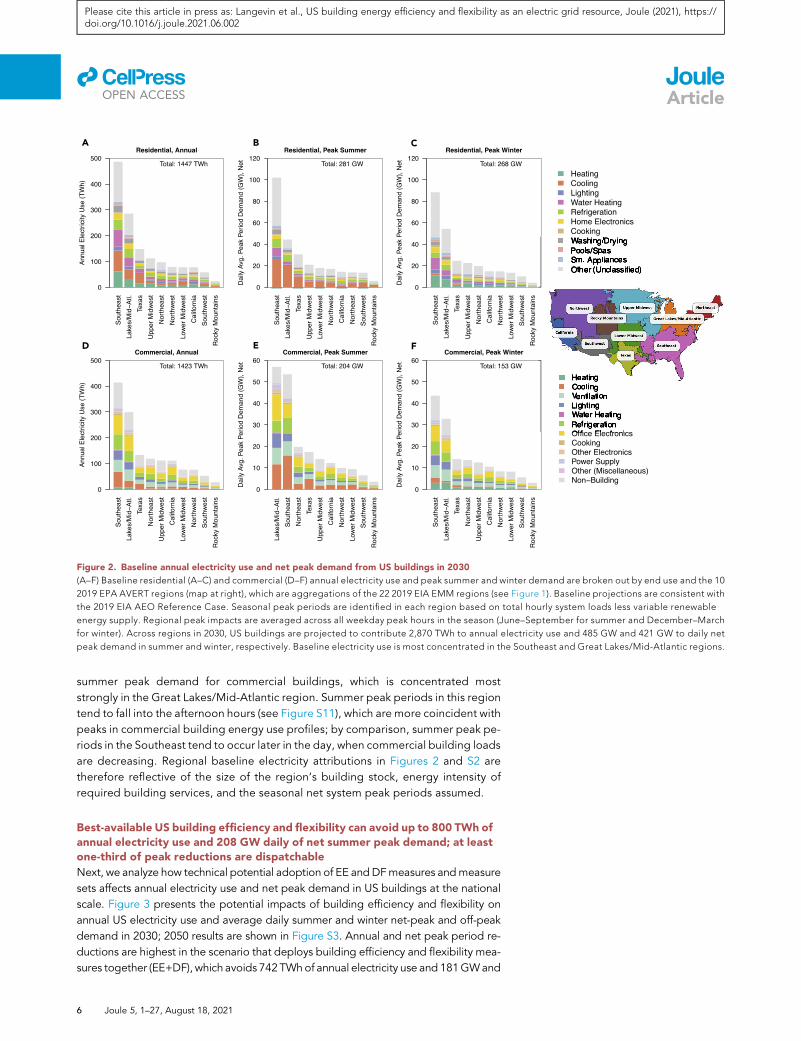
mand in US buildings across end uses and regions. Figure 2 presents the annual elec-

tricity use and average daily summer and winter net peak demand from US buildings

in 2030; 2050 results are shown in Figure S2. In 2030, buildings are responsible for

2,870 TWh of annual electricity use (71% of the contiguous US annual total39) and

485 GW and 421 GW of summer and winter net peak demand, respectively. By

2050, these totals grow to 3,249 TWh, 562 GW, and 469 GW, respectively. Residen-

tial buildings account for the largest share across each of these metrics, and differ-

ences between residential and commercial buildings are greater in the case of

peak demand, where residential buildings contribute 1.4–1.5 times more peak sum-

mer and 1.7 times more peak winter demand than commercial buildings.

Figures 2 and S2 show that space conditioning end uses—in particular, residential

heating and cooling and commercial cooling—are key drivers of 2030 and 2050

annual electricity use and net peak demand. Other end uses that make large contri-

butions across the metrics shown include water heating, refrigeration, and home

electronics in residential buildings and office electronics, refrigeration, and ventila-

tion in commercial buildings. Notably, a sizable portion of both residential and com-

mercial loads fall into the ‘‘unclassified’’ or ‘‘non-building’’ categories, which include

end uses that are not captured by EIA surveys40 and commercial loads such as water

distribution pumps, street lighting, and telecommunication; such categories are not

readily addressed by building efficiency or flexibility measures and thus limit the po-

tential magnitude of the building-grid resource.

Geographically, US building electricity use and peak demand are strongly concen-

trated in the Great Lakes/Mid-Atlantic and Southeast AVERT regions. These regions

aggregate multiple EMM regions with high population density, building square

footage, and annual electricity use (see Figure S1).40–42 In the Southeast, annual

electricity use and peak demand are further driven by significant cooling needs

and a large installed base of electric heating.40,42,43 While baseline electricity use

and peak demand tend to be highest in the Southeast, a notable exception is

Joule 5, 1–27, August 18, 2021 5

A B C

D E F

Figure 2. Baseline annual electricity use and net peak demand from US buildings in 2030

(A–F) Baseline residential (A–C) and commercial (D–F) annual electricity use and peak summer and winter demand are broken out by end use and the 10

2019 EPA AVERT regions (map at right), which are aggregations of the 22 2019 EIA EMM regions (see Figure 1). Baseline projections are consistent with

the 2019 EIA AEO Reference Case. Seasonal peak periods are identified in each region based on total hourly system loads less variable renewable

energy supply. Regional peak impacts are averaged across all weekday peak hours in the season (June–September for summer and December–March

for winter). Across regions in 2030, US buildings are projected to contribute 2,870 TWh to annual electricity use and 485 GW and 421 GW to daily net

peak demand in summer and winter, respectively. Baseline electricity use is most concentrated in the Southeast and Great Lakes/Mid-Atlantic regions.

llOPEN ACCESS


Article

summer peak demand for commercial buildings, which is concentrated most

strongly in the Great Lakes/Mid-Atlantic region. Summer peak periods in this region

tend to fall into the afternoon hours (see Figure S11), which are more coincident with

peaks in commercial building energy use profiles; by comparison, summer peak pe-

riods in the Southeast tend to occur later in the day, when commercial building loads

are decreasing. Regional baseline electricity attributions in Figures 2 and S2 are

therefore reflective of the size of the region’s building stock, energy intensity of

required building services, and the seasonal net system peak periods assumed.

Best-available US building efficiency and flexibility can avoid up to 800 TWh of

annual electricity use and 208 GW daily of net summer peak demand; at least

one-third of peak reductions are dispatchable

Next, we analyze how technical potential adoption of EE andDFmeasures andmeasure

sets affects annual electricity use and net peak demand in US buildings at the national

scale. Figure 3 presents the potential impacts of building efficiency and flexibility on

annual US electricity use and average daily summer and winter net-peak and off-peak

demand in 2030; 2050 results are shown in Figure S3. Annual and net peak period re-

ductions are highest in the scenario that deploys building efficiency and flexibility mea-

sures together (EE+DF), which avoids 742TWhof annual electricity use and 181GWand

6 Joule 5, 1–27, August 18, 2021

A B C

D E F

Figure 3. National impacts of best available building efficiency and flexibility measure sets on US annual electricity use and net peak and off-peak

demand in 2030

(A–F) Technical potential efficiency and flexibility impacts on residential annual electricity use (A), peak demand (B), and off-peak demand (C) are broken

out by end use and season alongside the same results for commercial buildings (D–F). Impacts are aggregated across the 22 2019 EIA EMM regions (see

Figure 1), and peak impacts are non-coincident across these regions. Seasonal peak and off-peak periods are identified in each underlying region based

on total hourly system loads less variable renewable energy supply; regional peak and off-peak impacts are averaged across all weekday peak and off-

peak hours in the season (June–September for summer and December–March for winter). In 2030, when deployed together, US building efficiency and

flexibility measures (EE+DF) can avoid up to 742 TWh annual electricity use and 181 GW daily peak demand, but also decrease off-peak demand by up to

79 GW. Flexibility without efficiency (DF) can add up to 13 GW to off-peak demand, with most of the increase observed in residential buildings.

llOPEN ACCESS


Article

119 GW of summer and winter net peak demand in 2030, respectively. By 2050, these

reductions grow to 800 TWh annual and 208 GW and 121 GW summer and winter net

peak, respectively. The annual reductions are 32% and 30% of total projected US fossil-

fired generation in 2030 and 2050, respectively, while the summer peak reductions in

these years are 26% and 22% of total projected fossil-fired capacity and 122% and

50% of new capacity additions after 202024; this suggests that aggressive deployment

of building efficiency and flexibility would substantially offset future needs for fossil-fired

base and peak load generation.Moreover, at least 59GWof summer peak reductions in

the EE+DF scenario are attributed to dispatchable flexibility measures, growing to 69

GW by 2050; the dispatchable portion of the EE+DF reductions is calculated by sub-

tracting efficiency-only scenario (EE) results from efficiency and flexibility scenario

(EE+DF) results. In the flexibility-only scenario (DF), the dispatchable resource reaches

96 GW in 2030 and 112 GW by 2050. By comparison, the EIA projects diurnal battery

storage to grow to up to 98GWby 205024; thus, the dispatchable resource we estimate

from building flexibility in 2050 is 70%–114% of EIA’s most optimistic storage capacity

projections for that year and constitutes a significant alternative to energy storage

deployment.

Across measure scenarios and projection years, residential buildings drive both

annual and peak reductions, primarily throughmeasures that affect cooling, heating,

and water heating. In commercial buildings, measures that affect office electronics

Joule 5, 1–27, August 18, 2021 7

llOPEN ACCESS


Article

show consistently high relative impacts across metrics—particularly annual and

winter peak reductions—while cooling measures dominate reductions in summer

peak demand. The relative attribution of annual and peak reductions to specific

end uses and building types mirrors the baseline distributions in Figures 2 and S2,

which are therefore key to understanding the prominence of particular efficiency

and flexibility measure impacts.

Increases in building demand during off-peak hours—those hours with the lowest

net system loads—are muted in Figures 3 and S3, reaching totals of up to just 13

GW in 2030 and 14 GW in 2050 in the DF scenario. The vast majority of the increases

(up to 13 GW) come from residential measures that shift water heating demand into

the off-peak hours; ice storage measures for cooling in large commercial buildings

contribute the second highest increase (up to 2 GW in summer). This finding high-

lights the challenges of marrying realistic building-level operational adjustments

with regional system net load balancing needs. To maximize effectiveness, for

example, precoolingmeasures reduce setpoint temperatures in the hours preceding

the peak hour window; however, the net utility load is low only for these hours in re-

gions with high midday solar generation (Figure S11). Potential load increases from

precooling would be more beneficial in a high solar penetration case where regions’

low net system loads occur during midday hours (see the sensitivity analysis in exper-

imental procedures). Thermal storage measures such as grid-responsive water heat-

ing and ice storage offer more potential for demand increases during off-peak pe-

riods but concentrate these increases in just a few hours, far fewer than the total

number of low net demand hours characteristic of many regions’ systems. Adding

to these inherent limitations of the flexibility measures, the introduction of efficiency

measures (EE+DF) counters additional off-peak demand by reducing the available

load for flexibility measures to shift, thus reducing off-peak-hour demand by up to

79 GW in 2030 and 88 GW in 2050.

Relative load reductions from efficiency and flexibility are largest in

residential buildings located in the South/Southeast and Great Lakes/Mid-

Atlantic regions in the summer season, though impacts vary widely across

geography and time

Third, we attribute the impacts of building efficiency and flexibility to specific US grid

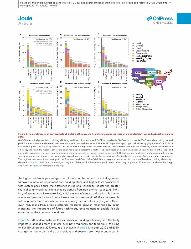
regions and sub-annual time periods. Figure 4 shows regional annual electricity use

and average daily summer and winter net peak demand reduction potentials for the

EE+DF scenario in 2030; 2050 results are shown in Figure S4. Regional variation in

annual electricity and peak demand reductions is mostly consistent with the baseline

variations across regions in Figures 2 and S2, again demonstrating the importance of

baseline system characteristics in determining the technical potential impacts of our

measure sets. In absolute terms, potential reductions are concentrated in the South-

east and the Great Lakes/Mid-Atlantic AVERT regions, consistent with the concen-

tration of baseline electricity use in these regions. In relative terms, percentage

reductions in Texas and the Southeast tend to be among the highest—particularly

in residential buildings—due to the stronger influence of reductions in cooling, heat-

ing, and water heating in these regions. Relative summer peak reductions are also

notably high for residential buildings in the Great Lakes/Mid-Atlantic region, where

temporal coincidence between afternoon system peaks and the residential cooling

peak results in large cooling electricity reductions relative to the total addressable

summer peak load.

Regional reduction percentages in Figures 4 and S4 tend to be higher and more var-

iable between regions in residential buildings than in commercial buildings. While

8 Joule 5, 1–27, August 18, 2021

A B C

D E F

Figure 4. Regional impacts of best available US building efficiency and flexibility measures together on annual electricity use and net peak demand in

2030

(A–F) The technical potential of building efficiency and flexibility measures (EE+DF) on residential (A–C) and commercial (D–F) annual electricity use and

peak summer and winter demand are broken out by end use and the 10 2019 EPA AVERT regions (map at right), which are aggregations of the 22 2019

EIA EMM regions (see Figure 1). Labels at the top of each bar represent the percentage of total addressable baseline electricity that is avoided by the

efficiency and flexibility measure set for the given region and assessment metric; the ‘‘addressable’’ baseline excludes unclassified residential loads and

non-building commercial loads. Seasonal peak periods are identified in each region based on total hourly system loads less variable renewable energy

supply; regional peak impacts are averaged across all weekday peak hours in the season (June–September for summer, December–March for winter).

The regional concentration of savings in the Southeast and Great Lakes/Mid-Atlantic regions mirror the distribution of baseline building electricity

demand in Figure 2. Reduction percentages are generally largest for the summer peak metric, when they range from 43%–67% in residential buildings

and from 43%–51% in commercial buildings.

llOPEN ACCESS


Article

the higher residential percentages stem from a number of factors including slower

turnover in baseline equipment and building stock and higher load coincidence

with system peak hours, the difference in regional variability reflects the greater

share of commercial reductions that are derived from non-thermal loads (e.g., light-

ing, refrigeration, office electronics), which are less influenced by location. Strikingly,

annual and peak reductions from office electronics measures in 2030 are comparable

with or greater than those of commercial cooling measures for many regions. More-

over, reductions from office electronics measures grow in magnitude by 2050,

indicating the importance of future technology development to enable flexible

operation of this commercial end use.

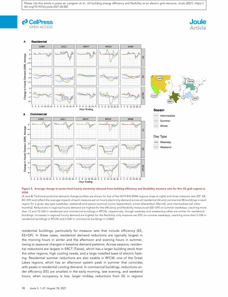
Figure 5 further demonstrates the variability of building efficiency and flexibility

impacts in 2030 at a more granular level, both regionally and temporally, focusing

on five EMM regions; 2050 results are shown in Figure S5. In both 2030 and 2050,

changes in hourly demand across regions and seasons are most pronounced in

Joule 5, 1–27, August 18, 2021 9

A

B

Figure 5. Average change in sector-level hourly electricity demand from building efficiency and flexibility measure sets for five US grid regions in

2030

(A and B) Technical potential demand change profiles are shown for five of the 2019 EIA EMM regions (map at right) and three measure sets (DF, EE,

EE+DF) and reflect the average impacts of each measure set on hourly electricity demand across all residential (A) and commercial (B) buildings in each

region for a given day type (weekday, weekend) and season (summer [June–September], winter [December–March]), and intermediate [all other

months]). Reductions in regional hourly demand are highest for the efficiency and flexibility measure set (EE+DF) on summer weekdays, reaching more

than 12 and 10 GW in residential and commercial buildings in RFCW, respectively, though weekday and weekend profiles are similar for residential

buildings. Increases in regional hourly demand are highest for the flexibility-only measure set (DF) on summer weekdays, reaching more than 5 GW in

residential buildings in RFCW and 2 GW in commercial buildings in CAMX.

llOPEN ACCESS


Article

residential buildings, particularly for measure sets that include efficiency (EE,

EE+DF). In these cases, residential demand reductions are typically largest in

the morning hours in winter and the afternoon and evening hours in summer,

owing to seasonal changes in baseline demand patterns. Across seasons, residen-

tial reductions are largest in ERCT (Texas), which has a larger building stock than

the other regions, high cooling needs, and a large installed base of electric heat-

ing. Residential summer reductions are also sizable in RFCW, one of the Great

Lakes regions, which has an afternoon system peak in summer that coincides

with peaks in residential cooling demand. In commercial buildings, reductions un-

der efficiency (EE) are smallest in the early morning, late evening, and weekend

hours, when occupancy is low; larger midday reductions from EE in regions

10 Joule 5, 1–27, August 18, 2021

A

B

Figure 6. Individual efficiency and flexibility measures with the largest summer net peak demand intensity reductions for five US grid regions in 2030

(A and B) The five individual efficiency (EE) or flexibility (DF) measures with the largest technical potential reductions in residential (A) and commercial (B)

summer peak demand intensity are highlighted for five of the 2019 EIA EMM regions (map at right). Measure impacts on summer peak demand (top row

of each panel) are shown alongside their impacts on winter peak demand (middle row) and annual electricity use (bottom row). Seasonal peak periods

llOPEN ACCESS

Joule 5, 1–27, August 18, 2021 11


Article

Figure 6. Continued

are identified in each region based on total hourly system loads less variable renewable energy supply; regional peak impacts are averaged across all

weekday peak hours in the season (June–September for summer and December–March for winter). Individual measures on the x axes are grouped into

general measure types shown in the plot legends. Preconditioning and HVAC equipment measures yield the largest summer peak reductions in

residential buildings while precooling and plug-load efficiency measures yield the largest summer peak reductions in commercial buildings.

Commercial plug-load efficiency also yields strong reductions across the winter peak and annual metrics.

llOPEN ACCESS


Article

with high solar penetration (e.g., CAMX) highlight the potential for efficiency

deployment to counter load-building objectives during hours of low net system

demand. Increases in commercial demand under flexibility (DF) are also more

regionally consistent and temporally constrained than in residential, occurring

mostly in the summer during the hours preceding the regional system peak

period, when precooling occurs.

Residential preconditioning as well as heat pump water heaters and

commercial plug load management are among the individual measures with

the largest impacts on electricity demand

Finally, we analyze which individual building efficiency (EE) or flexibility (DF) mea-

sures have the largest potential impacts on electricity demand in specific regions.

Figure 6 identifies the five residential and commercial measures with the largest im-

pacts on daily summer net peak demand intensity (W/ft2) in 2030 in each of the five

EMM regions from Figure 5; 2050 results are shown in Figure S6. In both figures, the

measures’ net winter peak demand and annual electricity reductions are also shown

to allow comparisons across metrics. In residential buildings, HVAC measures (con-

trols and equipment) generally deliver the largest summer peak reductions across

regions, led by preconditioning; preconditioning and other flexibility measures yield

no change or a slight increase in annual energy use, however. Peak reductions from

efficient air-source heat pumps (ASHPs) are prominent in the South and Southeast

(ERCT and SRSE), where ASHPs replace a large base of existing less-efficient heat

pumps and other electric heating; in the Northwest and Great Lakes (NWPP,

RFCW), however, baseline heating is predominantly gas, so central air conditioners

show more summer peak reduction potential. Outside of HVAC measures, heat

pump water heaters (HPWH) yield high summer peak-reductions across most re-

gions and are the top measure in California (CAMX), where the marine climate leads

to comparatively lower residential cooling needs in major population centers, and

the summer peak occurring late in the day places it past the time when cooling de-

mand is highest, thus reducing the potential for peak reduction from HVAC

measures.

In commercial buildings, plug-load efficiency (more efficient management of loads

from PCs and other office equipment) delivers the largest summer peak reduction

potential in three of the five regions. Savings from this measure are particularly pro-

nounced in the Great Lakes (RFCW), a further demonstration of the stronger coinci-

dence between this region’s afternoon system peak and commercial building load

profiles. Other measures that consistently rank in the top five across regions include

peak-period global temperature adjustments (GTA) with and without precooling,

lighting efficiency, and discharging of ice storage to meet peak cooling loads in

large commercial buildings. As with residential preconditioning, commercial

HVAC flexibility measures (precooling, ice storage) produce effectively no change

or slight increases in annual electricity use across regions. In contrast with the resi-

dential results, however, commercial measure impacts for California (CAMX) show

greater parity with those of the other regions, as the larger commercial baseline

load in California (see Figure 2) yields greater opportunity for peak reductions

from efficiency and flexibility measures.

12 Joule 5, 1–27, August 18, 2021

llOPEN ACCESS


Article

DISCUSSION

Our assessment demonstrates a large potential grid resource from energy-efficient

and flexible building operations that could be of high value to grid operators in

avoiding future fossil-fired generation investments and relieving pressure on energy

storage deployments to support variable renewable energy integration. Specifically,

if one values the estimated technical potential annual electricity reductions from ef-

ficiency and flexibility in 2030 and 2050 as early retirements of remaining coal gen-

eration, and assumes nondispatchable and dispatchable net peak reductions from

efficiency and flexibility avoid combined cycle gas and energy storage capacity ad-

ditions, respectively, the total building-grid resource is worth roughly $31 billion in

2030 and $42 billion in 2050.24,44,45 These estimates do not include additional ben-

efits to the grid such as avoided transmission and distribution infrastructure, reduced

greenhouse gas emissions, and reduced air pollution.46,47

Our analysis suggests that packaging efficiency and flexibility measures yields the

largest reductions in net peak electricity demand with comparable annual electricity

savings to an efficiency-only case; such packages may be simpler and more cost-

effective for utilities to market and can increase the value proposition of building ef-

ficiency and flexibility from a consumer perspective.48–50 On the other hand, we find

that packaging efficiency with flexibility limits the potential to shift demand into

hours of low net system load, when increased electricity demand from buildings

could improve the utilization of renewable energy supply. Efficiency generally re-

duces the load available to shift across the measure sets considered, as other recent

studies have demonstrated,51 though this may not be the case for individual effi-

ciency and flexibility packages that comprise themeasure sets.52 In a high renewable

penetration future, load reductions from efficiency could help avoid increases in

thermal generator cycling and ramping during low net system load periods, when

the net load is more variable; undoubtedly, however, avoiding renewable curtail-

ment during these periods through load shifting will also be a key challenge.53

Accordingly, emerging loads such as electric vehicle charging54 might need to be

leveraged to supplement the limited load shifting resource we estimate from

buildings.

The magnitudes of our estimated demand reductions appear broadly consistent

with existing studies at the regional level, though differences in approach and out-

puts preclude direct comparisons with previous work. For example, a study of the

US Eastern Interconnection estimates 97 GW peak demand reductions from effi-

ciency and flexibility measures by 2030 (versus 137 GW in corresponding regions

in our study); however, this study is an estimate of achievable potential, not technical

potential.55 Another study of DR potential in California finds that peak reductions in

the state could reach 6–8 GW by 2025 (versus 9 GW by 2030 in our results); however,

this estimate includes the industrial sector and focuses on ‘‘cost-competitive’’ DR.56

In the Southeast region, Nadel57 estimates up to 40 GW of summer and winter peak-

demand reductions from incremental efficiency improvements and DR in 2030

(versus 53 GW summer and 40 GW winter peak reductions in our study); again,

however, this study is not a technical potential analysis and it does not consider in-

teractions across efficiency and flexibility measures. The Northwest Power and Con-

servation Council’s (NPCC) Seventh Power Plan58 finds up to 9.9 GW summer and

13.2 GW winter peak reduction potential from efficiency and flexibility in 2035

(versus 10 GW summer and 7 GW winter peak reductions in our study’s Northwest

region results for 2030); however, the NPCC territory excludes southern parts of

our Northwest region, where cooling needs are greater. Importantly, all of these

Joule 5, 1–27, August 18, 2021 13

llOPEN ACCESS


Article

previous studies report peak reductions in terms of total system peak, whereas our

analysis averages net peak-hour impacts across all days in a season to estimate

potential.

Our estimates of the grid resource from building efficiency and flexibility would in-

crease with more aggressive electrification of end-use loads, which recent

studies suggest is necessary to achieve net-zero emissions from buildings by

midcentury.59,60 For example, under an illustrative case in which all fossil-fired heat-

ing, water heating, and cooking is switched to electric equipment at a baseline effi-

ciency level by 2050 (see experimental procedures), we find that annual electricity

use increases by 1,081 TWh (33%), while daily net peak loads increase by 231 GW

(49%) and 64 GW (11%) in the winter and summer, respectively (Figure S7). These re-

sults imply a new daily winter net peak of 700 GW that is 1.12 times larger than that of

the summer months in 2050. The majority of electrified load additions are attributed

to the heating end use, which, when considered independently, raises the daily net

peak load in the winter by 161 GW (1.12 times summer peak) and could raise it by as

much as 353 GW (1.46 times summer peak) if low-temperature degradation in heat

pump performance is so significant as to require full electric resistance at peak

heating demand (see discussion in experimental procedures and Figure S9). Co-

deployment of best available heating and water heating efficiency and flexibility

measures avoids 337 TWh (31%), 101 GW (44%), and 29 GW (45%) of the added

annual, winter peak, and summer peak loads, respectively (Figure S8), effectively

lowering the new winter-summer peak ratio to 1. Further study of the degree to

which electrification affects the building-grid resource is warranted, however, as

there is little to benchmark these estimates against. For instance, one recent study

finds a somewhat larger winter-summer peak ratio of 1.6 from full heating electrifi-

cation given the same regional aggregation (Table S4 in that study),61 but the ratio

is computed based on historical building heating and cooling needs (rather than

projected needs in 2050), reflects total buildings peak (rather than daily net system

peak), and includes detailed accounting for heating performance degradation at low

temperatures, all of which affords greater peak influence from electrifying fossil-fired

heating than in our modeling approach.

Finally, our results reflect a technical potential assessment of the building-grid

resource. The economic potential—accounting for electricity system benefits and

costs of the EE and DF measures—would likely fall short of the technical potential62

because not all of the measures are necessarily cost effective from the utility

perspective. Introducing realistic building and technology stock turnover and mar-

ket penetration dynamics would also reduce our impact estimates—possibly up to

two-thirds in the near-term (see experimental procedures). Important questions

remain about which economic and policy levers would be most effective in acceler-

ating adoption of the technology measures we consider; these might include utility

incentives, voluntary recognition programs (e.g., ENERGY STAR + Connected), co-

des and standards, and variable electricity tariffs, among others. Accordingly, while

the current analysis establishes the potential size and distribution of the building-

grid resource, follow-on analyses are needed to identify the most promising path-

ways and policy mechanisms for realizing this resource in the coming years.

EXPERIMENTAL PROCEDURES

Resource availability

Lead contact

Further information and requests for resources should be directed to the lead con-

tact, Jared Langevin ([email protected])

14 Joule 5, 1–27, August 18, 2021


llOPEN ACCESS


Article

Materials availability

No materials were used in this study.

Data and code availability

The code used to generate the paper’s results, results data, and supporting data sets

are available at https://doi.org/10.5281/zenodo.4737655.

Model overview

Estimates of building efficiency and flexibility potential were generated using a hybrid

building stock energy modeling approach that incorporates both top-down and bot-

tom-up elements.63Development of potential estimates follows four steps: (1) definition

of building efficiency and flexibility measures sets, (2) determination of regional power

system needs, (3) development of hourly end-use load profiles at the building-level for

representative locations and building types, with and without measures applied, and (4)

scaling of baseline and measure end-use load profiles across the building stock within

each modeled region. The following subsections outline key information for reproduc-

ing ourmethods; further details about certainmethodological elements are found in the

supplemental experimental procedures section.

Building efficiency and flexibility measures

Measures, as listed in Table 2, modify the baseline electricity demand profile of res-

idential and commercial buildings by improving upon the efficiency of baseline

building equipment, envelope, and/or controls (EE measure set); modifying base-

line operational schedules in response to regional power system conditions (DF

measure set); or by packaging these two types of changes (efficiency and flexibility

(EE+DF) measure set). Detailed measure definitions are provided in section S4, and

example building-level impacts from these three measure sets are shown in

Figure S20.

All EE measures adhere to a ‘‘best commercially available’’ energy performance

level. For residential buildings, best available performance is determined using

the Scout Core Measures Scenario Analysis data set and the National Residential

Efficiency Measures Database.64,65 For commercial buildings, best available per-

formance corresponds to the ASHRAE 50% Advanced Energy Design Guides

(AEDG) specifications. Where a 50% AEDG guideline is not available for a certain

building type, the most applicable 30% AEDG guideline is used instead (see sec-

tion S4.2.1).

Efficiency measures cover all major end uses across the residential and commercial

sectors (heating/cooling, ventilation, lighting, refrigeration, and water heating), as

well as home and office electronics (TVs, personal and work computers, and related

equipment); residential efficiency measures additionally address several smaller elec-

tric appliance loads such as clothes washers, clothes dryers, dishwashers, and pool

pumps. Across building types, envelope efficiency packages are assessed that imple-

ment higher performance opaque envelope components (walls, roof, floors), highly

insulating windows, and air sealing; operational control measures are also represented

(smart thermostats in residential, daylighting and occupancy controls in commercial).

DF measures implement load shedding (for example, dimming the lights) or load shift-

ing (for example, decreasing cooling setpoints in the hours leading up to the peak de-

mand period to enable ‘‘coasting’’ with higher setpoints during the peak period, or

charging thermal energy storage overnight to use to meet cooling setpoints later in

the day). All flexibility measures modify baseline loads in the most aggressive manner

Joule 5, 1–27, August 18, 2021 15

https://doi.org/10.5281/zenodo.4737655

Table 2. Residential and commercial measure definitions.

Measure set Name Building type(s) End use(s) Description

EE

envelope insulation and air sealing res + com heating and cooling current best available technology–––––––

HVAC equipment res + com heating and cooling

lighting res + com lighting

electronics res + com home and office electronics

refrigeration res + com refrigeration

appliances residential washing and drying

water heater residential water heating (WH)

pool pumps residential pools and spas

thermostat controls residential heating and cooling fixed increase or decrease of temperaturesduring unoccupied and nighttime hours

DF

global temperature adjustment (GTA) commercial HVAC increase or decrease zone temperature setpointsduring peak hours

GTA + precooling res + com cooling (res + com), ventilation (com) decrease zone setpoints in the 4 h prior to peakperiod, then float temperature setpoint duringpeak hours

GTA + preheating residential heating increase zone setpoints prior to peak period thenfloat temperature setpoint during peak hours

GTA + precooling + thermal storage commercial HVAC charge ice storage overnight and dischargeduring peak hours; limited to large commercial

continuous dimming commercial lighting dim lighting and shut off lighting in unoccupiedspaces during peak hours

low priority device switching commercial office electronics switch off low-priority devices (e.g., unused PCs,office equipment) during peak hours

appliance demand response residential washing and drying shift appliance loads before or after peak hours

water heating demand response residential water heating preheat water heater setpoint during off-peakhours on the grid

electronics demand response residential home electronics shift a fraction of plug loads to before or afterpeak hours

pool pumps demand response residential pools and spas shift peak-hour pool pump loads to off-peakhours on the grid

EE+DF

GTA + pre-cool/heat + efficient envelope &HVAC equipment; daylighting controls +dimming

commercial HVAC and lighting combine DF HVAC and lighting strategies withmore efficient envelope and equipment,daylighting, and controls

thermostat controls + pre-cool/heat + efficientenvelope and HVAC equipment

residential heating and cooling combine DF heating and cooling strategies withmore efficient envelope and equipment

non-thermostat DR + EE residential WH, lighting, home electronics, refrigeration,washing and drying, pools and spas

shift WH and appliance loads outside of peakhours; upgrade appliances and WHs to bestavailable efficient technology

device switching + efficient electronics commercial office electronics combine DF electronics strategy with the mostefficient PCs and office equipment

all remaining EE ECMs commercial refrigeration, WH account for efficiency measures that are not apart of the packaged EE+DF measures above

See supplemental experimental procedures section 4 for additional details.

llOPEN

ACCESS

16

Joule

5,1–2

7,August

18,2021

Please

citethisarticle

inpress

as:La

ngevin

etal.,

USbuild

ingenergyefficie

ncy

andflexib

ilityasanelectric

grid

reso

urce

,Jo

ule

(2021),http

s://doi.o

rg/10.1016/j.jo

ule.2021.06.002

Article

llOPEN ACCESS


Article

possible without compromising basic building service needs, where service thresholds

are determined on a load-by-load basis as described further in section S4.2.2. Specific

operational schedules for the flexibility measures—the hour ranges during which load

shedding and shifting is required—are determined by regional power system condi-

tions as described in the next sub-section.

Flexibility measures address the residential and commercial electric loads that are

the largest contributors to annual electricity demand and can potentially be shed

or shifted in response to daily power system needs. In residential buildings, this in-

cludes heating, cooling, water heating, appliances (clothes washing, clothes drying,

dishwashing, pool pumps) and electronics; in commercial buildings, this includes

heating, cooling, ventilation, lighting, refrigeration, and office electronics (PCs

and office equipment).

Energy efficiency and DF measures are packaged (EE+DF) to explore possible inter-

active effects between these measure types, for example: (1) efficiency measures

reduce the available load shedding and shifting potential of flexibility measures,

and (2) efficiency measures enhance the effectiveness of thermal flexibility mea-

sures—e.g., through envelope upgrades that extend the effects of precooling or dis-

charging of thermal energy storage. In developing the measure sets, respective ef-

ficiency and flexibility measures are combined without additional modifications. For

example, when precooling measures are packaged with a more efficient envelope,

we do not assume any additional thermostat setback potential for the packaged

version of these measures.

Regional power system conditions

When scaled across the building stock, each of the efficiency and flexibility measure

sets considered in our analysis has a collective impact on electricity demand at the

regional power system level. Accordingly, measure impacts at the building level

are designed and assessed relative to typical daily power system conditions and ob-

jectives, namely: (1) reduce building electricity demand during times of high total

system load with low renewable electricity supply, when marginal electricity costs

are likely to be highest; and (2) shift peak electricity demand into times with lower

total system load and abundant renewable electricity supply, when marginal elec-

tricity costs are likely to be lowest. These objectives are best illustrated by examining

the net system load shape in a given region, which subtracts total hourly variable

renewable electricity generation from total hourly electricity demand across the re-

gion. Measure sets that target net system peak reduction and load shifting needs

yield a net system load shape that is lower and flatter than that of a baseline demand

scenario. Such load shapes benefit utility operators by reducing the need for peak

load capacity investments, avoiding daily curtailments of renewable electricity sup-

ply, and mitigating the need to bring generators on and offline rapidly to meet sud-

den changes in net demand.66,67

We assess our measure sets’ potential to affect net system load shapes in the 22

2019 EIA EMM regions, which cover the contiguous US68 Using regional EMM sys-

tem load and generation data provided by EIA for the 2019 AEO Reference Case,

which covered every five (5) projection years from 2020–2050, we first develop

peak-normalized net system load profiles for each region (r), projection year (y),

month (m), day type (d), and hour of the day (hd), lnetr ;y;m;d;hd :

lnetr;y;m;d;hd =Lnetr ;y;m;d;hd

max1%m%12Lnetr ;y;m;d;hd

; (Equation 1)

Joule 5, 1–27, August 18, 2021 17

llOPEN ACCESS


Article

Lnetr;y;m;d;hd = Ltotr;y;m;d;hd � Lrgenr ;y;m;d;hd ; (Equation 2)

where Lnetr;y;m;d;hd is the net system load, max1%m%12Lnetr;y;m;d;hd is the maximum value of

the net system load in region r and projection year y across all months, day types

(weekday, weekend, and peak day per EMM convention39), and hours, and the net

load is derived by subtracting total renewable solar and wind generation Lrgenr ;y;m;d;hd

from total system load, Ltotr ;y;m;d;hd .

Next, we calculate the average of the normalized net system load profiles from

Equation 1 across each combination of region (r), season (s), and hour of the day

(hd), lnet

r ;s;hd :

lnet

r ;s;hd =XMs

m= 1

XDd = 1

�lnetr ;y =2050;m;d;hd

�wd;m; (Equation 3)

where Ms is the set of months belonging to season s (summer [Jun–Sep]; winter [Dec–

Mar]; intermediate [all other months]), D is the set of three EMM day types (weekday,

weekend, peak day), and wd;m is the averaging weight for the combination of day

typed andmonthm, defined as its proportion of the total number of days in a given sea-

son.Note that Equation 3 is based on the net system load profiles for the year 2050 only;

2050 is chosen because it is the year inwhich renewable penetration is at its highest satu-

ration in the EIA data (29%); section S2.1.1 explores the implications of higher renewable

penetration on our definition of system conditions and associated measure impacts,

showing limited sensitivities that mostly concern the definition of low net load periods.

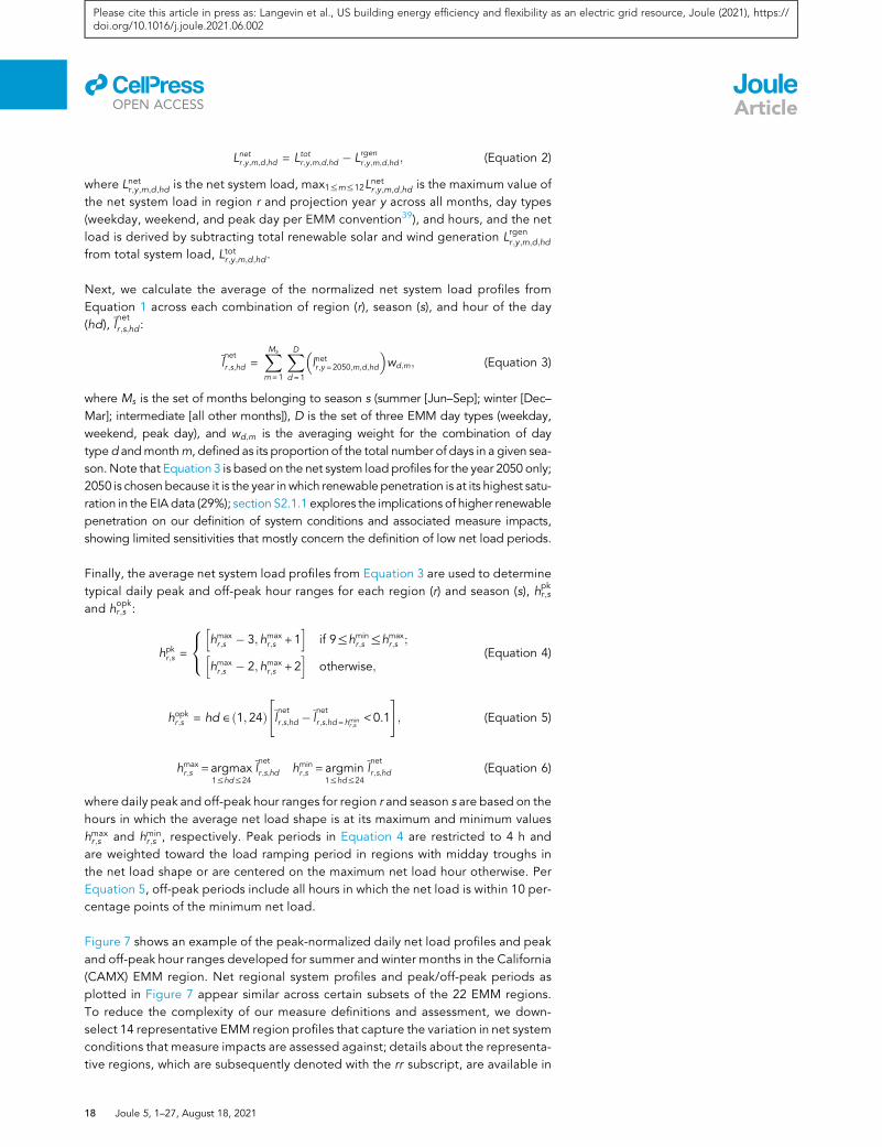
Finally, the average net system load profiles from Equation 3 are used to determine

typical daily peak and off-peak hour ranges for each region (r) and season (s), hpkr ;s

and hopkr;s :

hpkr;s =

8<:

hhmaxr ;s � 3;hmax

r;s + 1i

if 9%hminr;s %hmax

r ;s ;hhmaxr ;s � 2;hmax

r;s + 2i

otherwise;(Equation 4)

hopkr ;s = hd ˛ð1; 24Þ

"lnet

r;s;hd � lnet

r ;s;hd = hminr ;s

<0:1

#; (Equation 5)

hmaxr;s = argmax

1%hd%24

lnet

r ;s;hd hminr;s = argmin

1%hd%24

lnet

r;s;hd (Equation 6)

where daily peak and off-peak hour ranges for region r and season s are based on the

hours in which the average net load shape is at its maximum and minimum values

hmaxr;s and hmin

r ;s , respectively. Peak periods in Equation 4 are restricted to 4 h and

are weighted toward the load ramping period in regions with midday troughs in

the net load shape or are centered on the maximum net load hour otherwise. Per

Equation 5, off-peak periods include all hours in which the net load is within 10 per-

centage points of the minimum net load.

Figure 7 shows an example of the peak-normalized daily net load profiles and peak

and off-peak hour ranges developed for summer and winter months in the California

(CAMX) EMM region. Net regional system profiles and peak/off-peak periods as

plotted in Figure 7 appear similar across certain subsets of the 22 EMM regions.

To reduce the complexity of our measure definitions and assessment, we down-

select 14 representative EMM region profiles that capture the variation in net system

conditions that measure impacts are assessed against; details about the representa-

tive regions, which are subsequently denoted with the rr subscript, are available in

18 Joule 5, 1–27, August 18, 2021

A B

Figure 7. Peak-normalized total system loads net variable renewable energy generation for the

California (CAMX) grid region

(A and B) Typical daily net load shapes are shown for all months in the summer (A) and winter (B)

seasons. Seasonal peak and off-peak net load periods are constructed for this and all

representative utility regions in our analysis (see Figure S11); CAMX is used to define grid

conditions in ASHRAE climate zone 3C as indicated by the plot titles. The peak load period is

defined as 4 h surrounding the maximum net load hour, while the off-peak window is defined as all

hours in which the normalized net system load is within 10 percentage points of the minimum net

system load for the given season. Peak and off-peak hour ranges are represented as horizontal line

segments on the plots, with maximum andminimum load hours (averaged across all load shapes for

the season) marked as single points on the plots. All normalized net load profiles are based on the

year 2050, which is the year with the highest projected renewable penetration in EIA EMM

modeling for the 2019 Annual Energy Outlook.69 In CAMX, the large midday trough in the net load

shapes reflect the high degree of solar generation projected for this region, which pushes net peak

loads later into the evening hours.

llOPEN ACCESS


Article

Table S3; daily net load profiles are shown for all 14 representative regions in

Figure S11.

End-use load profiles at the building level

Assessment of efficiency and flexibility measure impacts begins at the building level,

where EnergyPlus70 simulations of hourly building energy loads under baseline op-

erations and with the measure sets applied are used to develop hourly load savings

shapes for eachmeasure in the analysis. Baseline load simulations in EnergyPlus cap-

ture the effects of changes in weather (using typical meteorological year [TMY3]

data71), building occupancy, and equipment operation schedules in constraining

the available load for efficiency and flexibility measures to affect in a particular

hour of the year, building type, and location. Hourly energy use results from Energy-

Plus have been validated against empirical data for multiple buildings and thus serve

as useful baselines for our analysis of measure impacts for individual buildings,

though important caveats about the use of EnergyPlus are noted in the analysis lim-

itations sub-section.72–75

Simulation models are developed for a representative city in each of the 14 contig-

uous US ASHRAE 90.1–2016 climate zones76 and for six building types that are

chosen to represent variations in typical end-use load shape patterns across the res-

idential and commercial building stock. Single-family homes, which comprise the

strong majority of residential square footage and electricity use (84% and 82% in

2020, respectively24), are used as the representative residential building type. Com-

mercial building usage and load patterns are more diverse than residential and thus

require a larger set of representative building types—we use medium and large of-

fices, large hotels, standalone retail, and warehouses. Further justification for

Joule 5, 1–27, August 18, 2021 19

llOPEN ACCESS


Article

the choice of these representative commercial building types is provided in

section S2.2.1.

EnergyPlus simulations of residential loads are conducted using ResStock, an anal-

ysis tool that allows for characterization and energy modeling of diverse single-fam-

ily detached homes in the United States. ResStock generates baseline EnergyPlus

building energy models through a sampling routine that assigns region-specific

home characteristics and accounts for the diversity in vintage, construction proper-

ties, installed equipment, appliances, and occupant behavior within a region. Data

for the baseline home properties come from numerous sources, including the

2009 Residential Energy Consumption Survey (RECS).77 After generating the base-

line buildingmodels, ResStock leverages physics-based energy modeling in Energy-

Plus and high-performance computing to simulate each baseline home, as well as

homes with efficiency and flexibility measures applied. Approximately 10,000 resi-

dential building models are generated for each representative city. By modeling

many homes, we capture the diversity in the existing residential building stock

and provide a highly granular view of residential energy usage with EE and DF mea-

sures applied. Further details regarding the methodology behind ResStock can be

found in Wilson et al.78

Commercial buildings loads are simulated using the commercial prototype models

developed by the US Department of Energy to support assessment and compliance

with local building codes.79 The prototype models represent a cross section of com-

mon commercial building types covering 80% of new commercial construction80; our

analysis uses the Large Office, Medium Office, Stand-alone Retail, Large Hotel, and

Warehouse (non-refrigerated) prototypes, which map to the full set of prototypes as

shown in Table S4 and explained further in section S2.2.1. While multiple prototype

construction vintages are available, we limit our simulations to the 2004 vintage,

which best balances the expected evolution in typical commercial construction char-

acteristics across the projected time horizon (2015–2050, covered in the next sub-

section). EnergyPlus files for simulating the baseline case and measure sets are

generated using the OpenStudio Measures capability, which automates the process

of EnergyPlus model creation and modification. Baseline prototype files are gener-

ated using the existing Create DOE Prototype Building Measure,81 while new Mea-

sures are developed to represent the particular sets of commercial building effi-

ciency and flexibility measures assessed in this paper. Further details regarding

the development and assumptions of the commercial prototype models can be

found in Goel et al.82 and Thornton et al.,80 while additional details about OpenStu-

dio Measures are available in Roth et al.83

Across the residential and commercial contexts examined, hourly EnergyPlus loads

for each measure are translated to hourly load savings fractions for a given ASHRAE

climate zone (c), representative EMM region (rr ), representative EnergyPlus building

type (bre), end use (u), and hour of the year (hy), Dlmeasc;rr;bre;u;hy :

Dlmeasc;rr ;bre;u;hy = lmeas

c;rr ;bre;u;hy � lbasec;rr ;bre;u;hy ; (Equation 7)

lbasec;rr ;bre;u;hy =Lbasec;rr ;bre;u;hyP8760

hy = 1Lbasec;rr ;bre;u;hy

; (Equation 8)

lmeasc;rr;bre;u;hy =

Lmeasc;rr ;bre;u;hyP8760

hy = 1Lbasec;rr ;bre;u;hy

(Equation 9)

20 Joule 5, 1–27, August 18, 2021

llOPEN ACCESS


Article

where lbasec;rr ;bre;u;hy and lmeasc;rr ;bre;u;hy are the hourly end-use fractions of annual load under

the baseline case and with measurem applied, and Lbasec;rr;bre;u;hy and Lmeasc;rr;bre;u;hy are the

total (unnormalized) hourly EnergyPlus load outputs for the given combination of

climate, EMM region, representative EnergyPlus building type (bre), and end

use, under the baseline and measure case, respectively. All EnergyPlus outputs

reflect a non-leap year that begins on a Sunday and are reported in local standard

time.

Per Table S3, building-level measure savings profiles for each ASHRAE climate zone

(c) may address the net system load profiles of up to two representative EMM re-

gions (rr ). Note, however, that regional power system conditions only influence

the building-level results for energy flexibility (DF) or packaged efficiency and flexi-

bility (EE+DF) measures, which modify baseline building loads non-uniformly across

hours under the objective of shedding load during system net peak hours and shift-

ing load to off-peak hours as described in the previous sub-section and in Table 2; by

contrast, efficiency-only (EE) measures reduce loads uniformly across hours regard-

less of system conditions.

Building-level simulations of the measures in Table 2 account for interactive effects

across certain efficiency and flexibility components in the analysis by packaging

these components in the simulations—by co-simulating envelope and HVAC equip-

ment improvements, for example. This practice ensures that aggregation of

resultant measure savings shapes across a portfolio (e.g., to develop results for Fig-

ures 3, 4, 5, and S3–S5) avoids double-counting the impacts of contributing

measures. We also simulate disaggregated versions of packaged measures—for

example, we simulate an envelope improvement made independently of an HVAC

equipment improvement, and vice versa. This parallel practice allows exploration

of individual measure impacts in isolation, as in Figures 6 and S6.

End-use load profiles at the regional power system level

To scale the effects of building-level measure application to the regional power sys-

tem level, we use Scout (scout.energy.gov)—an openly available modeling software

originally developed to estimate the short- and long-term annual impacts of building

energy efficiency on US energy use, CO2 emissions, and operating costs. Previous

Scout analyses have assessed these metrics on an annual basis for different climate

zones or the US as a whole84; here, we adapt Scout to integrate hourly data on

regional power system conditions and building-level efficiency and flexibility im-

pacts with annual projections of building sector electricity use and demand out to

2050. Further details regarding Scout’s general methodological approach can be

found in the Supplemental Experimental Procedures of Langevin et al.84; an initial

effort to translate Scout’s annual data sets to a sub-annual temporal resolution,

which the current work builds upon, is reported in Satre-Meloy and Langevin.85

First, Scout generates annual projections of building electricity use by EMM region

(r) and AEO building type (b), end use (u), technology type (t), and projection year (y),

Ebaser ;b;u;t;y , drawing from AEO 2019 Reference Case projections of building electricity

from 2015–2050 that are resolved by census division (cd):

Ebaser ;b;u;t;y =

XCDcd = 1

Ebasecd;b;u;t;ywcd (Equation 10)

where Ecd;b;u;t;y is the AEO 2019-projected electricity use of the given building type,

end use, and technology type in census division cd and year y, and wcd is an EIA

Joule 5, 1–27, August 18, 2021 21

http://scout.energy.gov

llOPEN ACCESS


Article

building electricity sales-based mapping factor that determines the portion of

census division cd that falls in EMM region r. Mapping factors are reported for res-

idential and commercial buildings in Tables S5 and S6, respectively; these factors are

also used to translate AEO-projected residential and commercial building square

footages from a census division to EMM region resolution, for the purpose of

normalizing measure load impacts by floor area as in Figures 6 and S6. Note that

Scout’s building types (3 residential; 11 commercial), end uses (14 residential; 10

commercial) and technology types are consistent with those used in the AEO.39

EMM-resolved segments of baseline building electricity use from Equation 10 are

then multiplied by hourly measure load savings fractions (Equation 7) for the appro-

priate ASHRAE climate zone (c), representative EMM region (rr ), EnergyPlus building

type (bre), and end use (u), yielding hourly load savings estimates for each measure

when applied to the given baseline segment, DEmeasr ;b;u;t;y;hy :

DEmeasr;b;u;t;y;hy =

XCc =1

XBbe= 1

Ebaser;b;u;t;yDl

measc;rr1r;bre1be;u;hywcwbe (Equation 11)

where wc and wbre are mapping factors that determine the portion of ASHRAE

climate zone c that falls into EMM region r and the portion of EnergyPlus building

type be that comprises AEO building type b, respectively; the mappings between

ASHRAE and EMM regions and between EnergyPlus and AEO building types are re-

ported in Tables S7 and S8. For a given EMM region r, the associated representative

region rr in the hourly measure load savings fraction term Dlmeasc;rr1r;bre1be;u;hy is

selected based on the mapping between representative EMM regions and the full

set of EMM regions each represents in Table S3. In the same term, the representative

EnergyPlus building type bre for a given EnergyPlus building type be is selected

based on the mapping between representative EnergyPlus building types and the

full set of EnergyPlus building types each represents in Table S4.

The final step in the Scout calculations determines the annual and seasonal daily

average net peak and off-peak impacts of each measure in each EMM region,

DEmeasr;b;u;t;y , DE

meas; pkr;b;u;t;y;s;dw , and DE

meas; opkr;b;u;t;y;s;dw :

DEmeasr ;b;u;t;y =

X8760hy = 1

DEmeasr;b;u;t;y;hy (Equation 12)

DEmeas; pkr;b;u;t;y;s;dw =

X8760hy = 1

8>><>>:

DEmeasr ;b;u;t;y;hy

Npkr;s;dw

if hy ˛Hpkr;s;dw

0 otherwise

(Equation 13)

DEmeas; opkr ;b;u;t;y;s;dw =

X8760hy =1

8>><>>:

DEmeasr;b;u;t;y;hy

Nopkr;s;dw

if hy ˛Hopkr;s;dw

0 otherwise

(Equation 14)

whereHpkr;s;dw andH

opkr;s;dw are the sets of hours that fall under the season s, day type dw

(weekday, weekend), and daily peak and off-peak hour ranges for region r in season s

(hpkr;s and h

opkr ;s from Equations 4 and 5, respectively), andN

pkr ;s;dw and N

opkr;s;dw are the to-

tal numbers of hours in Hpkr;s;d and H

opkr ;s;d , respectively.

The Scout calculations yieldmeasure impacts on stock-level electricity use (TWh) and

demand (GW) that are resolved by EMM region, Scout/AEO building type, and end-

use technology class; these results can be aggregated into the higher-level AVERT

22 Joule 5, 1–27, August 18, 2021

llOPEN ACCESS


Article

regions (Figure 1), residential and commercial building breakouts, and end-use-level

results presented throughout.

Analysis limitations

Key methodological limitations are grouped into those concerning building-level

measure simulations and those concerning the representation of regional electricity

system needs.

At the building scale, our analysis relies on EnergyPlus-simulated baseline end-use

load shapes and measure impacts rather than electricity meter data or device-level

measured electricity use data because these data are not available across the broad

array of measure types and locations considered in this study; metered data for our

measure sets is a particular challenge since we investigate the operation of technol-

ogies that are not yet widely adopted. As mentioned, previous work has validated

hourly EnergyPlus simulations against empirical data72–75; nevertheless, we

acknowledge important limitations in the methods employed with EnergyPlus in

this study. In particular, we use a representative subset of building types to account

for variations in baseline load profiles across the US building stock (see section S2.2);

these building type models rely on either a set of operating schedules or a single

schedule to represent occupancy and thermostat setpoints. To the extent that

real-world operational schedules are more diverse than what is represented in our

analysis, this difference might translate to greater diversity in baseline loads and,

therefore, increase and/or decrease the potential load impacts of efficiency and flex-

ibility measures. In the summer months, for example, greater diversity in residential

building occupancy and thermostat setpoint schedules could lower the peak period

potential from residential cooling measures by reducing the concentration of base-

line cooling loads around the evening hours; conversely, increased schedule diver-

sity for most commercial buildings could add cooling loads to these evening hours,

thus increasing the potential for load reductions from efficiency and flexibility. While

this limitation is important, the end-use load shapes used in this study constitute a

significant improvement over current publicly available load shape data with na-

tional coverage,86 which are far less granular in terms of building types and temporal

resolution, and we expect to update our analysis with the outputs of ongoing work to

develop calibrated end-use load profiles of the entire US building stock.87

Three additional limitations apply at the building scale. First, we use a single represen-

tative city in each climate zone to capture the impacts of weather on simulatedmeasure

impacts; previous research has shown that in some cases, use of multiple representa-

tive cities within each climate zone is warranted to improve the accuracy of estimated

electricity use patterns.88 Moreover, the TMY3 weather inputs to our building-level

simulations do not encompass the most extreme variations in hourly weather patterns

within a given year or represent the effects of current warming trends71 or the expec-

tation that thosewarming trendswill continue in the future.Our results thus exclude the

option value of flexibility under more extreme weather and system loads.89 Finally, our

analysis holds hourly distributions of baseline end-use loads and the relative load im-

pacts of best available building efficiency and flexibility constant across the simulated

time horizon (2015–2050). In practice, changes to these load distributions and relative

measure impacts could be expected—for example, with new patterns of building use if

more people work from home, or with decreasing differences between ‘‘typical’’ and

best available building technologies on the market over time.

At the utility scale, our use of high and low net system load periods as a proxy for grid

needs has its own limitations. First, net load shape magnitudes alone do not fully

Joule 5, 1–27, August 18, 2021 23

llOPEN ACCESS


Article

encapsulate themany factors that can drive temporal variations in the value of efficiency

and flexibility to the electric grid, including fuel supply constraints, power plant availabil-

ity, and regulatory factors.90,91 Second, the spatiotemporal granularity of our net system

load shapes is limited to a subset of representative regions (Table S3) and typical day

types within each season, which maymiss some of the variation in these net load shapes

that would be captured by a higher spatiotemporal resolution. Finally, the scope of our

analysis excludes a number of additional grid value streams for building efficiency and

flexibility, including: mitigation of load ramping, which is defined by the rate of change

of load with time rather than its absolute minimum and maximum; coordination of flex-

ible loads in buildings with distributed energy resources (DERs), which might offer more

potential value at specific distribution system locations and enable greater building-

level resilience not reflected in our analysis; and fast response services such as load

modulating for frequency regulation, which could offer additional benefits.92

SUPPLEMENTAL INFORMATION

Supplemental information can be found online at https://doi.org/10.1016/j.joule.

2021.06.002.

ACKNOWLEDGMENTS

This work was authored by The Regents of the University of California under contract

no. DE-AC02-05CH11231 and by the Alliance for Sustainable Energy, LLC, the man-

ager and operator of the National Renewable Energy Laboratory for the US Depart-

ment of Energy (DOE) under contract no. DE-AC36-08GO28308. Funding was pro-

vided by US Department of Energy Office of Energy Efficiency and Renewable

Energy Building Technologies Office. The views expressed in the article do not

necessarily represent the views of the DOE or the US Government. A portion of

this research was performed using computational resources sponsored by the US

Department of Energy’s Office of Energy Efficiency and Renewable Energy and

located at the National Renewable Energy Laboratory. The authors gratefully

acknowledge the assistance of Laura Martin and Kevin Jarzomski, US Energy Infor-

mation Administration (EIA), in accessing EIA NEMS Electricity Market Module

and Buildings Module data, respectively. The authors appreciate the thoughtful

comments of multiple external reviewers of this work.

AUTHOR CONTRIBUTIONS

Conceptualization, J.L. and C.B.H.; methodology, J.L., C.B.H., A.S.-M., H.C.-P.,

A.S., E.P., R.A., and E.J.H.W.; investigation, J.L., C.B.H., H.C.-P., A.S., E.P., and

R.A.; writing – original draft, J.L., A.S.M., A.S., and H.C.-P.; writing – review & edit-

ing, J.L., A.S.-M., C.B.H., A.J.S., and E.J.H.W.; validation, J.L., C.B.H., A.S.-M.,

H.C.-P., and A.S.; formal analysis, J.L., C.B.H., A.S.-M., H.C.-P., and A.S., visualiza-

tion, J.L., A.S.-M., and C.B.H.; software, J.L., H.C.-P., A.S., E.P., and R.A.; resources,

E.J.H.W.; data curation, J.L. and C.B.H.; supervision, J.L., C.B.H., E.J.H.W., and

A.J.S.; project administration, J.L. and C.B.H.; funding acquisition, J.L. and C.B.H.

DECLARATION OF INTERESTS

The authors declare no competing interests.

Received: January 5, 2021

Revised: March 15, 2021

Accepted: June 8, 2021

Published: July 7, 2021

24 Joule 5, 1–27, August 18, 2021



llOPEN ACCESS


Article

REFERENCES

1. BNEF (2021). 2021 Sustainable Energy inAmerica Factbook, (Bloomberg New EnergyFinance). https://bcse.org/factbook/.

2. BNEF (2019). New Energy Outlook 2019,(Bloomberg New Energy Finance). https://about.bnef.com/new-energy-outlook/.

3. Goldman School of Public Policy (2020). 2035The Report: Plummeting solar, wind andbattery costs can accelerate our cleanelectricity future (University of CaliforniaBerkeley Goldman School of Public Policy).https://www.2035report.com/wp-content/uploads/2020/06/2035-Report.pdf.

4. Creutzig, F., Roy, J., Lamb, W.F., Azevedo,I.M.L., Bruine de Bruin, W., Dalkmann, H.,Edelenbosch, O.Y., Geels, F.W., Grubler, A.,Hepburn, C., et al. (2018). Towards demand-side solutions for mitigating climate change.Nature Clim. Change 8, 260–263.

5. Grubler, A.,Wilson, C., Bento, N., Boza-Kiss, B.,Krey, V., McCollum, D.L., Rao, N.D., Riahi, K.,Rogelj, J., De Stercke, S., et al. (2018). A lowenergy demand scenario for meeting the1.5 �C target and sustainable developmentgoals without negative emission technologies.Nat. Energy 3, 515–527.

6. Mundaca, L., Urge-Vorsatz, D., and Wilson, C.(2019). Demand-side approaches for limitingglobal warming to 1.5�C. Energy Effic 12,343–362.

7. Wilson, C., Pettifor, H., Cassar, E., Kerr, L., andWilson, M. (2019). The potential contribution ofdisruptive low-carbon innovations to 1.5�Cclimate mitigation. Energy Effic 12, 423–440.

8. Sorrell, S. (2015). Reducing energy demand: areview of issues, challenges and approaches.Renew. Sustain. Energy Rev. 47, 74–82.

9. Jensen, S.Ø., Marszal-Pomianowska, A., Lollini,R., Pasut, W., Knotzer, A., Engelmann, P.,Stafford, A., and Reynders, G. (2017a). IEA EBCannex 67 energy flexible buildings. EnergyBuild 155, 25–34.

10. Jensen, S.Ø., Madsen, H., Lopes, R., Junker,R.G., Aelenei, D., Li, R., Metzger, S., Lindberg,K.B., Marszal, A.J., Kummert, M., et al. (2017b).Annex 67: Energy Flexible Buildings(International Energy Agency). https://www.annex67.org/.

11. Cappers, P., Mills, A., Goldman, C., Wiser, R.,and Eto, J.H. (2012). An assessment of the rolemass market demand response could play incontributing to the management of variablegeneration integration issues. Energy Policy 48,420–429.

12. Lund, P.D., Lindgren, J., Mikkola, J., andSalpakari, J. (2015). Review of energy systemflexibility measures to enable high levels ofvariable renewable electricity. Renew. Sustain.Energy Rev. 45, 785–807.

13. Dyson,M., Mandel, J., Lehrman, M., Bronski, P.,Morris, J., Palazzi, T., Ramirez, S., and Touati, H.(2015). The economics of demand flexibility:how ‘‘flexiwatts’’ create quantifiable value forcustomers and the grid, (Rocky MountainInstitute). https://rmi.org/wp-content/uploads/2017/05/RMI_Document_Repository_Public-Reprts_RMI-

TheEconomicsofDemandFlexibilityFullReport.pdf.

14. Goldenberg, C., Dyson, M., and Masters, H.(2018). Demand flexibility: the key to enabling alow-cost, low-carbon grid, (Rocky MountainInstitute). https://rmi.org/wp-content/uploads/2018/02/Insight_Brief_Demand_Flexibility_2018.pdf.

15. Hale, E.T., Bird, L.A., Padmanabhan, R., andVolpi, C.M. (2018). Potential roles for demandresponse in high-growth electric systems withincreasing shares of renewable generation,National Renewable Energy Laboratory. NREL/TP–6A20-70630. https://www.nrel.gov/docs/fy19osti/70630.pdf.

16. Mai, T., Sandor, D., Wiser, R., and Schneider, T.(2012). Renewable electricity futures study:executive summary, National RenewableEnergy Laboratory. NREL/TP-6A20-52409-ES.https://www.nrel.gov/docs/fy13osti/52409-ES.pdf.

17. Strbac, G. (2008). Demand side management:benefits and challenges. Energy Policy 36,4419–4426.

18. Bradley, P., Leach, M., and Torriti, J. (2013). Areview of the costs and benefits of demandresponse for electricity in the UK. Energy Policy52, 312–327.

19. O’Connell, N., Pinson, P., Madsen, H., andO’Malley, M. (2014). Benefits and challenges ofelectrical demand response: a critical review.Renew. Sustain. Energy Rev. 39, 686–699.

20. Aunedi, M., Kountouriotis, P.-A., Calderon,J.E.O., Angeli, D., and Strbac, G. (2013).Economic and environmental benefits ofdynamic demand in providing frequencyregulation. IEEE Trans. Smart Grid 4, 2036–2048.

21. Wang, F., Xu, H., Xu, T., Li, K., Shafie-Khah, M.,and Catalao, J.P.S. (2017). The values ofmarket-based demand response on improvingpower system reliability under extremecircumstances. Appl. Energy 193, 220–231.

22. Siano, P., and Sarno, D. (2016). Assessing thebenefits of residential demand response in areal time distribution energy market. Appl.Energy 161, 533–551.

23. FERC (2020). FERC order no. 2222: a new dayfor distributed energy resources, FederalEnergy Regulatory Commission. https://www.ferc.gov/media/ferc-order-no-2222-fact-sheet.

24. EIA (2020). Annual Energy Outlook 2020 withprojections to 2050, US Energy InformationAdministration. https://www.eia.gov/outlooks/aeo/pdf/AEO2020%20Full%20Report.pdf.

25. Neukomm, M., Nubbe, V., and Fares, R. (2019).Grid- interactive efficient buildings: overview,United States Department of Energy. https://www.energy.gov/eere/buildings/grid-interactive-efficient-buildings.

26. FERC (2009). A national assessment of demandresponse potential, Federal Energy RegulatoryCommission. https://www.ferc.gov/sites/default/files/2020-05/06-09-demand-response_1.pdf.

27. EPRI (2009). Assessment of achievablepotential from energy efficiency and demandresponse programs in the U.S. (2010 - 2030),Electric Power Research Institute. https://www.epri.com/research/products/1016987.

28. Hledik, R., Faruqui, A., Lee, T., and Higham, J.(2019). The national potential for load flexibility:value and market potential through 2030, TheBrattle Group. https://brattlefiles.blob.core.windows.net/files/16639_national_potential_for_load_flexibility_-_final.pdf.

29. Huang, S., Ye, Y., Wu, D., and Zuo, W. (2021).An assessment of power flexibility fromcommercial building cooling systems in theUnited States. Energy 221, 119571.

30. Paterakis, N.G., Erdinc, O., and Catalao, J.P.S.(2017). An overview of demand response: key-elements and international experience. Renew.Sustain. Energy Rev. 69, 871–891.

31. Zhang, S., Jiao, Y., and Chen, W. (2017).Demand-side management (DSM) in theContext of China’s on-Going Power SectorReform. Energy Policy 100, 1–8.

32. Chen, Y., Xu, P., Gu, J., Schmidt, F., and Li, W.(2018). Measures to improve energy demandflexibility in buildings for demand response(DR): a review. Energy Build 177, 125–139.

33. Li, R., and You, S. (2018). Exploring potential ofenergy flexibility in buildings for energy systemservices. CSEE JPES 4, 434–443.

34. Gils, H.C. (2014). Assessment of the theoreticaldemand response potential in Europe. Energy67, 1–18.

35. Kies, A., Schyska, B.U., and Von Bremen, L.(2016). The demand side managementpotential to balance a highly renewableEuropean power system. Energies 9, 955.

36. Soder, L., Lund, P.D., Koduvere, H., Bolkesjø,T.F., Rossebø, G.H., Rosenlund-Soysal, E.,Skytte, K., Katz, J., and Blumberga, D. (2018). Areview of demand side flexibility potential innorthern Europe. Renew. Sustain. Energy Rev.91, 654–664.

37. DOE (2005). The value of economic dispatch. Areport to Congress pursuant to section 1234 ofthe Energy Policy Act of 2005, US Departmentof Energy. https://www.energy.gov/sites/default/files/oeprod/DocumentsandMedia/value.pdf.

38. Stern, F. (2013). Chapter 10: peak demand andtime-differentiated energy savings cross-cutting protocols: the uniform methodsproject: methods for determining energyefficiency savings for specific measures,National Renewable Energy Laboratory.https://www.nrel.gov/docs/fy17osti/68566.pdf.

39. EIA (2019). Annual Energy Outlook 2019 withprojections to 2050, US Energy InformationAdministration. https://www.nrel.gov/docs/fy17osti/68566.pdf.

40. EIA (2018). 2015 residential energyconsumption survey data, US EnergyInformation Administration. https://www.eia.gov/consumption/residential/data/2015/.

Joule 5, 1–27, August 18, 2021 25

https://bcse.org/factbook/

https://about.bnef.com/new-energy-outlook/

https://about.bnef.com/new-energy-outlook/

https://www.2035report.com/wp-content/uploads/2020/06/2035-Report.pdf

https://www.2035report.com/wp-content/uploads/2020/06/2035-Report.pdf

http://refhub.elsevier.com/S2542-4351(21)00290-7/sref4
































https://www.annex67.org/

https://www.annex67.org/












https://rmi.org/wp-content/uploads/2017/05/RMI_Document_Repository_Public-Reprts_RMI-TheEconomicsofDemandFlexibilityFullReport.pdf





https://rmi.org/wp-content/uploads/2018/02/Insight_Brief_Demand_Flexibility_2018.pdf



https://www.nrel.gov/docs/fy19osti/70630.pdf


https://www.nrel.gov/docs/fy13osti/52409-ES.pdf

https://www.nrel.gov/docs/fy13osti/52409-ES.pdf



























https://www.ferc.gov/media/ferc-order-no-2222-fact-sheet

https://www.ferc.gov/media/ferc-order-no-2222-fact-sheet

https://www.eia.gov/outlooks/aeo/pdf/AEO2020%20Full%20Report.pdf

https://www.eia.gov/outlooks/aeo/pdf/AEO2020%20Full%20Report.pdf

https://www.energy.gov/eere/buildings/grid-interactive-efficient-buildings



https://www.ferc.gov/sites/default/files/2020-05/06-09-demand-response_1.pdf



https://www.epri.com/research/products/1016987

https://www.epri.com/research/products/1016987

https://brattlefiles.blob.core.windows.net/files/16639_national_potential_for_load_flexibility_-_final.pdf



































https://www.energy.gov/sites/default/files/oeprod/DocumentsandMedia/value.pdf







https://www.eia.gov/consumption/residential/data/2015/


llOPEN ACCESS


Article

41. U.S. Census Bureau (2010). 2010 census results -United States and Puerto Rico populationdensity by county or county equivalent. https://www2.census.gov/geo/pdfs/maps-data/maps/thematic/us_popdensity_2010map.pdf.

42. EIA (2016). 2012 commercial buildings energyconsumption survey data, US EnergyInformation Administration. https://www.eia.gov/consumption/commercial/data/2012/.

43. EIA (2019). Units and calculators explained -degree days, US Energy InformationAdministration. https://www.eia.gov/energyexplained/units-and-calculators/degree-days.php.

44. EIA (2020a). Table 8.4. Average power plantoperating expenses for Major U.S. investor-owned electric utilities, 2009 through 2019(Mills per Kilowatthour), US Energy InformationAdministration. https://www.eia.gov/electricity/annual/html/epa_08_04.html.

45. EIA (2020b). U.S. battery storage markettrends, US Energy Information Administration.https://www.eia.gov/analysis/studies/electricity/batterystorage/.

46. EPA (2018). Quantifying themultiple benefits ofenergy efficiency and renewable energy: aguide for state and local governments, USEnvironmental Protection Agency. https://www.epa.gov/statelocalenergy/quantifying-multiple-benefits-energy-efficiency-and-renewable-energy-guide-state.

47. Langevin, J., Satre-Meloy, A., and Fadali, L.(2020). Attaching public health benefits tobuilding efficiency measures at the nationaland regional scales. In 2020 ACEEE SummerStudy on Energy Efficiency in Buildings, J.Granderson and D. Hun, eds. (LawrenceBerkeley National Laboratory), pp. 9-277–9-289.

48. Billimoria, S., Henchen, M., Guccione, L., andLouis-Prescott, L. (2018). The economics ofelectrifying buildings: how electric space andwater heating supports decarbonization ofresidential buildings, Rocky Mountain Institute.https://rmi.org/insight/the-economics-of-electrifying-buildings/.

49. Goldman, C., Reid, M., Levy, R., and Silverstein,A. (2010). Coordination of energy efficiencyand demand response, United StatesEnvironmental Protection Agency. https://emp.lbl.gov/publications/coordination-energy-efficiency-and.

50. York, D., Relf, G., and Waters, C. (2019).Integrated energy efficiency and demandresponse programs, American Council for AnEnergy Efficient Economy. https://www.aceee.org/research-report/u1906.

51. Weiss, T. (2020). Energy flexibility and shiftableheating power of building components andtechnologies. Smart Sustain. Built Environ.https://doi.org/10.1108/SASBE-09-2019-0128.

52. Gerke, B.F., Zhang, C., Satchwell, A., Murthy,S., Piette, M.A., Present, E., Wilson, E., Speake,A., and Adhikari, R. (2020). Modeling theinteraction between energy efficiency anddemand response on regional grid scales. In2020 ACEEE Summer Study on EnergyEfficiency in Buildings, J. Granderson and D.Hun, eds. (Lawrence Berkeley NationalLaboratory), pp. 9-137–9-152.

26 Joule 5, 1–27, August 18, 2021

53. Mai, T.T., Jadun, P., Logan, J.S., McMillan, C.A.,Muratori, M., Steinberg, D.C., Vimmerstedt,L.J., Haley, B., Jones, R., and Nelson, B. (2018).Electrification futures study: scenarios ofelectric technology adoption and powerconsumption for the United States, NREL/TP–6A20-71500 National Renewable EnergyLaboratory. https://www.nrel.gov/docs/fy18osti/71500.pdf.

54. Fitzgerald, G., Nelder, C., and Newcomb, J.(2016). Electric vehicles as distibuted energyresources, Rocky Mountain Institute. https://rmi.org/wp-content/uploads/2017/04/RMI_Electric_Vehicles_as_DERs_Final_V2.pdf.

55. Rohmund, I., Wikler, G., Kester, B., Ryan, B.,Marrin, K., Prijyanonda, J., Ghosh, D., Duer, A.,and Williamson, C. (2010). Assessment ofdemand response and energy efficiencypotential: volume 2 eastern interconnectionanalysis. 1314–2, Global Energy Partners, LLC.https://documents.pserc.wisc.edu/documents/publications/special_interest_publications/miso/Midwest-ISO_DR_and_EE_Potential_Assessment_Final_Volume%202.pdf.

56. Alstone, P., Potter, J., Piette, M.A., Schwartz, P.,Berger, M.A., Dunn, L.N., Smith, S.J., Sohn,M.D., Aghajanzadeh, A., Stensson, S., et al.(2016). 2015 California demand responsepotential study - charting California’s demandresponse future, Interim report on phase 1results. LBNL–2001115 Lawrence BerkeleyNational Laboratory. https://doi.org/10.2172/1421793.

57. Nadel, S. (2017). Electricity consumption andpeak demand scenarios for the SoutheasternUnited States. u1704, American Council for AnEnergy Efficient Economy. https://www.aceee.org/research-report/u1704.

58. NPCC (2016). Seventh Northwest conservationand electric power plan, Northwest Power andConservation Council. https://www.nwcouncil.org/reports/seventh-power-plan.

59. Williams, J.H., Jones, R.A., Haley, B., Kwok, G.,Hargreaves, J., Farber, J., and Torn, M.S.(2021). Carbon-neutral pathways for the UnitedStates. AGU Adv 2, 1–25.

60. National Academies of Sciences, Engineering,and Medicine (2021). Acceleratingdecarbonization of the U.S. energy system (TheNational Academies Press). https://www.nap.edu/catalog/25932/accelerating-decarbonization-of-the-us-energy-system.

61. Waite, M., and Modi, V. (2020). Electricity loadimplications of space heating decarbonizationpathways. Joule 4, 376–394.

62. Dranka, G.G., and Ferreira, P. (2019). Reviewand assessment of the different categories ofdemand response potentials. Energy 179,280–294.

63. Langevin, J., Reyna, J.L.,Ebrahimigharehbaghi, S., Sandberg, N.,Fennell, P., Nageli, C., Laverge, J., Delghust,M., Mata, E., Van Hove, M., et al. (2020a).Developing a common approach for classifyingbuilding stock energy models. Renew. Sustain.Energy Rev. 133, 110276.

64. Langevin, J., Harris, C.B., and Reyna, J.L.(2020b). Scout coremeasures scenario analysis.https://doi.org/10.5281/zenodo.3706923.

65. NREL (2018). National residential efficiencymeasures database, NREMDB v3.1.0. https://remdb.nrel.gov/.

66. Alstone, P., Potter, J., Piette, M.A., Schwartz, P.,Berger, M.A., Dunn, L.N., Smith, S.J., Sohn,M.D., Aghajanzadeh, A., Stensson, S., et al.(2017). 2025 California demand responsepotential study - charting California’s demandresponse future: final report on phase 2 results.LBNL-2001113, Lawrence Berkeley NationalLaboratory. https://buildings.lbl.gov/publications/2025-california-demand-response.

67. O’Connell, N., Hale, E., Doebber, I., andJorgenson, J. (2015). On the inclusion ofenergy- shifting demand response inproduction cost models: methodology and acase study, National Renewable EnergyLaboratory, NREL/TP-6A20-64465. https://www.nrel.gov/docs/fy15osti/64465.pdf.

68. EIA (2018). The National Energy ModelingSystem: an overview 2018, U.S. EnergyInformation Administration. https://www.eia.gov/outlooks/aeo/nems/overview/pdf/0581(2018).pdf.

69. EIA (2018). The electricity market module of thenational energy modeling system: modeldocumentation, US Energy InformationAdministration. https://www.eia.gov/outlooks/aeo/nems/documentation/electricity/pdf/m068(2018).pdf.

70. Crawley, D.B., Pedersen, C.O., Lawrie, L.K., andWinkelmann, F.C. (2000). EnergyPlus: energysimulation program. ASHRAE J 42, 49–56.

71. Wilcox, S., and Marion, W. (2008). User’smanual for TMY3 data sets, NationalRenewable Energy Laboratory NREL/TP-581-43156. https://www.nrel.gov/docs/fy08osti/43156.pdf.

72. Im, P., New, J.R., and Joe, J. (2019). Empiricalvalidation of building energy modeling usingflexible research platform. Proceedings of the16th IBPSA Conference, 4515–4521.

73. Li, Q., Muehleisen, R., Ravache, B., and Haves,P. (2019). Empirical validation of single-roomheat transfer models under uncertainty.Proceedings of the 16th IBPSAConference, pp.4715–4722.

74. Haves, P., Ravache, B., Fergadiotti, A., Kohler,C., and Yazdanian, M. (2019). Accuracy ofHVAC load predictions: validation ofEnergyPlus and DOE-2 using an instrumentedtest facility. Proceedings of the 16th IBPSAConference, pp. 4329–4336.

75. Haves, P., Ravache, B., and Yazdanian, M.(2020). Accuracy of HVAC load predictions:validation of EnergyPlus and DOE-2 usingFLEXLAB measurements (Lawrence BerkeleyNational Laboratory), pp. 45–52. https://doi.org/10.20357/B7H88D.

76. Liu, B., Rosenberg, M., and Athalye, R. (2018).National impact of ANSI/ASHRAE/IES.Standard 90.1-2016. Building PerformanceAnalysis Conference and SimBuild.

77. EIA (2013). 2009 residential energyconsumption survey, US Energy InformationAdministration. https://www.eia.gov/consumption/residential/data/2009/.

https://www2.census.gov/geo/pdfs/maps-data/maps/thematic/us_popdensity_2010map.pdf



https://www.eia.gov/consumption/commercial/data/2012/

https://www.eia.gov/consumption/commercial/data/2012/

https://www.eia.gov/energyexplained/units-and-calculators/degree-days.php



https://www.eia.gov/electricity/annual/html/epa_08_04.html

https://www.eia.gov/electricity/annual/html/epa_08_04.html

https://www.eia.gov/analysis/studies/electricity/batterystorage/

https://www.eia.gov/analysis/studies/electricity/batterystorage/

https://www.epa.gov/statelocalenergy/quantifying-multiple-benefits-energy-efficiency-and-renewable-energy-guide-state












https://rmi.org/insight/the-economics-of-electrifying-buildings/

https://rmi.org/insight/the-economics-of-electrifying-buildings/

https://emp.lbl.gov/publications/coordination-energy-efficiency-and



https://www.aceee.org/research-report/u1906


https://doi.org/10.1108/SASBE-09-2019-0128












https://rmi.org/wp-content/uploads/2017/04/RMI_Electric_Vehicles_as_DERs_Final_V2.pdf



https://documents.pserc.wisc.edu/documents/publications/special_interest_publications/miso/Midwest-ISO_DR_and_EE_Potential_Assessment_Final_Volume%202.pdf





https://doi.org/10.2172/1421793

https://doi.org/10.2172/1421793



https://www.nwcouncil.org/reports/seventh-power-plan

https://www.nwcouncil.org/reports/seventh-power-plan





https://www.nap.edu/catalog/25932/accelerating-decarbonization-of-the-us-energy-system

















https://doi.org/10.5281/zenodo.3706923

https://remdb.nrel.gov/

https://remdb.nrel.gov/

https://buildings.lbl.gov/publications/2025-california-demand-response





https://www.eia.gov/outlooks/aeo/nems/overview/pdf/0581(2018).pdf



https://www.eia.gov/outlooks/aeo/nems/documentation/electricity/pdf/m068(2018).pdf












https://doi.org/10.20357/B7H88D

https://doi.org/10.20357/B7H88D



llOPEN ACCESS


Article

78. Wilson, E.J., Christensen, C.B., Horowitz, S.G.,Robertson, J.J., and Maguire, J.B. (2017).Energy efficiency potential in the U.S. single-family housing stock, US Department ofEnergy. National Renewable EnergyLaboratory NREL/TP-5500-68670. https://www.nrel.gov/docs/fy18osti/68670.pdf.

79. DOE (2021). Commercial prototype buildingmodels. https://www.energycodes.gov/development/commercial/prototype_models.

80. Thornton, B.A., Rosenberg, M.T., Richman,E.E., Wang, W., Xie, Y., Zhang, J., Cho, H.,Heejin, V.V., Athalye, R.A., and Liu, B. (2011).Achieving the 30% goal: energy and costsavings analysis of ASHRAE standard 90.1-2010, Technical Report PNNL-20405 PacificNorthwest National Laboratory. https://www.energycodes.gov/achieving-30-goal-energy-and-cost-savings-analysis-ashrae-standard-901-2010.

81. NREL (2020). Create DOE prototype building.https://bcl.nrel.gov/node/83591.

82. Goel, S., Athalye, R.A., Wang, W., Zhang, J.,Rosenberg, M.I., Xie, Y., Hart, P.R., and

Mendon, V.V. (2014). Enhancements toASHRAE standard 90.1 prototype buildingmodels, Technical Report PNNL-23269, PacificNorthwest National Laboratory. https://www.osti.gov/biblio/1129366-enhancements-ashrae-standard-prototype-building-models.

83. Roth, A., Goldwasser, D., and Parker, A. (2016).There’s a measure for that! Energy Build 117,321–331.

84. Langevin, J., Harris, C.B., and Reyna, J.L. (2019).Assessing the potential to reduce U.S. buildingCO2 emissions 80% by 2050. Joule 3, 2403–2424.

85. Satre-Meloy, A., and Langevin, J. (2019).Assessing the time-sensitive impacts of energyefficiency and flexibility in the US buildingsector. Environ. Res. Lett. 14, 124012.

86. Electric Power Research Institute. (2021). EPRIload shape library 8.0. https://loadshape.epri.com/enduse.

87. NREL (2020). End-use load profiles for the U.S.building stock. https://www.nrel.gov/buildings/end-use-load-profiles.html.

88. Burleyson, C.D., Voisin, N., Taylor, Z.T., Xie, Y.,and Kraucunas, I. (2018). Simulated buildingenergy demand biases resulting from the useof representative weather stations. Appl.Energy 209, 516–528.

89. Sezgen, O., Goldman, C.A., and Krishnarao, P.(2007). Option value of electricity demandresponse. Energy 32, 108–119.

90. EIA (2020). Electricity explained: factorsaffecting electricity prices, US EnergyInformation Administration. https://www.eia.gov/energyexplained/electricity/prices-and-factors-affecting-prices.php.

91. Mills, A.D., Levin, T., Wiser, R., Seel, J., andBotterud, A. (2020). Impacts of variablerenewable energy on wholesale markets andgenerating assets in the United States: a reviewof expectations and evidence. Renew. Sustain.Energy Rev. 120, 109670.

92. Ma, O., Alkadi, N., Cappers, P., Denholm, P.,Dudley, J., Goli, S., Hummon, M., Kiliccote, S.,MacDonald, J., Matson, N., et al. (2013).Demand response for ancillary services. IEEETrans. Smart Grid 4, 1988–1995.

Joule 5, 1–27, August 18, 2021 27



https://www.energycodes.gov/development/commercial/prototype_models

https://www.energycodes.gov/development/commercial/prototype_models

https://www.energycodes.gov/achieving-30-goal-energy-and-cost-savings-analysis-ashrae-standard-901-2010




https://bcl.nrel.gov/node/83591

https://www.osti.gov/biblio/1129366-enhancements-ashrae-standard-prototype-building-models














https://loadshape.epri.com/enduse

https://loadshape.epri.com/enduse

https://www.nrel.gov/buildings/end-use-load-profiles.html

https://www.nrel.gov/buildings/end-use-load-profiles.html









https://www.eia.gov/energyexplained/electricity/prices-and-factors-affecting-prices.php














US building energy efficiency and flexibility as an ...

Documents

Transcript of US building energy efficiency and flexibility as an ...