Economics of global yield gaps: A spatial analysis

Uris Lantz C. Baldos and Thomas W. Hertel

Department of Agricultural Economics

Purdue University

West Lafayette, IN 47907-2056

E-mail: ubaldos@purdue.edu

Selected Paper prepared for presentation at the

Agricultural & Applied Economics Association’s 2012 AAEA Annual Meeting,

Seattle, Washington, August 12-14, 2012.

PRELIMINARY DRAFT – DO NOT CITE WITHOUT PERMISSION COMMENTS WELCOME

Copyright 2012 by Baldos and Hertel. All rights reserved. Readers may make verbatim copies

of this document for non-commercial purposes by any means, provided that this copyright

1

Economics of global yield gaps: A spatial analysis

Abstract

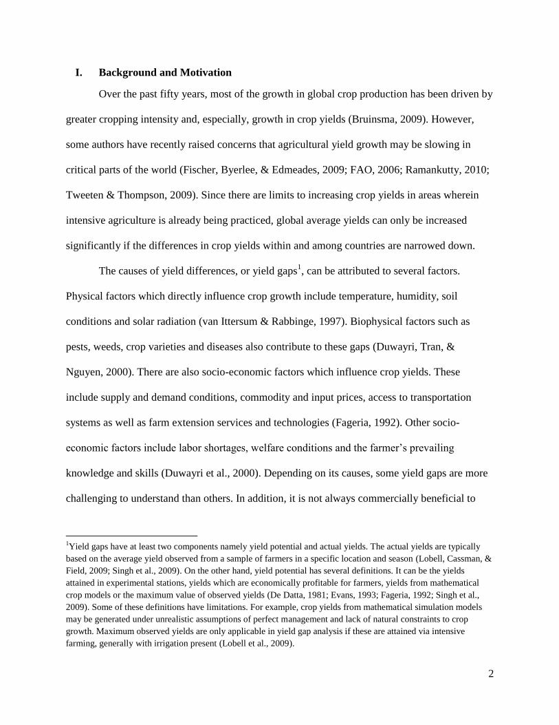
In this paper, we contribute to the existing literature of global yield gap analysis by using

geo-spatial dataset on crop yields, agro-climatic factors and selected socio-economic variables.

In line with the literature, we link yield gaps to technical efficiencies. By treating each grid-cell

as a farm unit, we employ data envelopment analysis to calculate relative farm efficiencies with

respect to a technically efficient global production frontier. We then apply spatial econometric

techniques to relate the calculated efficiency scores to population, irrigation, fertilizer use,

market access, institutional strength and market influence. We find that the effects of the socio-

economic variables on the efficiency scores are not consistent and will typically vary by

geographic region, crop type and on the scope of analysis (all areas, irrigated areas only, rainfed

areas only). However, we can see some general trends. Most of the total impacts of socio-

economic variables on efficiency scores are positive. For example, across all crops, regions and

all areas, estimates of the total impact of irrigation, fertilizer use, institutional strength and

market influence are generally positive. In regions wherein efficiency scores are low, the key

variables which positively affect these scores are market influence and fertilizer use. By

changing the coverage from all areas to either rainfed or irrigated areas, we generally see

changes in the statistical significance of some variables.

2

I. Background and Motivation

Over the past fifty years, most of the growth in global crop production has been driven by

greater cropping intensity and, especially, growth in crop yields (Bruinsma, 2009). However,

some authors have recently raised concerns that agricultural yield growth may be slowing in

critical parts of the world (Fischer, Byerlee, & Edmeades, 2009; FAO, 2006; Ramankutty, 2010;

Tweeten & Thompson, 2009). Since there are limits to increasing crop yields in areas wherein

intensive agriculture is already being practiced, global average yields can only be increased

significantly if the differences in crop yields within and among countries are narrowed down.

The causes of yield differences, or yield gaps1, can be attributed to several factors.

Physical factors which directly influence crop growth include temperature, humidity, soil

conditions and solar radiation (van Ittersum & Rabbinge, 1997). Biophysical factors such as

pests, weeds, crop varieties and diseases also contribute to these gaps (Duwayri, Tran, &

Nguyen, 2000). There are also socio-economic factors which influence crop yields. These

include supply and demand conditions, commodity and input prices, access to transportation

systems as well as farm extension services and technologies (Fageria, 1992). Other socio-

economic factors include labor shortages, welfare conditions and the farmer’s prevailing

knowledge and skills (Duwayri et al., 2000). Depending on its causes, some yield gaps are more

challenging to understand than others. In addition, it is not always commercially beneficial to

1Yield gaps have at least two components namely yield potential and actual yields. The actual yields are typically

based on the average yield observed from a sample of farmers in a specific location and season (Lobell, Cassman, &

Field, 2009; Singh et al., 2009). On the other hand, yield potential has several definitions. It can be the yields

attained in experimental stations, yields which are economically profitable for farmers, yields from mathematical

crop models or the maximum value of observed yields (De Datta, 1981; Evans, 1993; Fageria, 1992; Singh et al.,

2009). Some of these definitions have limitations. For example, crop yields from mathematical simulation models

may be generated under unrealistic assumptions of perfect management and lack of natural constraints to crop

growth. Maximum observed yields are only applicable in yield gap analysis if these are attained via intensive

farming, generally with irrigation present (Lobell et al., 2009).

3

close these gaps, especially if input costs are high, farmers have poor access to markets, and if

they face significant production risks (Evans, 1993; Herdt, 1979).Given these complications,

understanding the causes of yield gaps is critical.

In the literature, studies typically use crop production data collected at country, state or

regional level (Bravo-Ureta et al., 2006; FAO, 2000; Liu & Myers, 2008; Nisrane et al., 2011;

Sekhon et al., 2010; Singh et al., 2009). However, national level data can only provide

information on average yields even though there is great heterogeneity in yields within a country.

More recently, the availability of global data sets on crop yields at a grid cell level permits the

assessment of global yield gaps at a highly disaggregated level (Licker et al., 2010; Neumann et

al., 2010). However, to our knowledge, only the paper of Neumann et al (2010) use satellite data

in calculating and explaining yield gaps across the world. The authors used stochastic frontier

analysis (SFA) which is an econometric technique that has been widely used in estimating and

explaining farm inefficiencies which are directly related to crop yields gaps. The authors then

attributed the estimated inefficiencies to differences in land management practices. Proxy

variables used to capture the effects of land management practices include slope, irrigation,

population in the agricultural sector, as well as distance to markets (i.e. market accessibility) and

spatially disaggregated purchasing power parity (i.e. market influence).

Despite being innovative, the paper has some limitations. Some of the economic variables

considered in the study might not be appropriate proxy variables for land management practices.

For example, the authors defined market influence as measure of the suitability of yield-

improving investments in agriculture; hence, areas with greater market influence have higher

yields. The authors constructed the proxy for market influence using national data on purchasing

power parity (PPP) and distances to nearest markets (i.e. market access). However, PPP can only

4

provide information on the purchasing power of different currencies and it might not be a good

measure of farm investment suitability.

In addition, the authors did not take advantage of the spatial nature of the data. The

authors used the maximum likelihood technique proposed by Battese and Coelli (1995) in order

to estimate the production frontier and technical efficiencies. This approach which is tailored to

panel data assumes that the efficiency terms are independently distributed. However, given the

spatial nature of the data it is possible that the efficiency terms are correlated across space. As a

solution for this problem, the authors used an ad-hoc approach by extracting a random sample of

10% from the grid cells with at least 3% cropping area to ensure that each observation are

independent (i.e. reduced spatial autocorrelation). A better alternative is to model the spatial

autocorrelation in the data as a spatial stochastic process. Once modeled, the spatial interaction

of one location to other location can be used as an explanatory variable (Anselin, 2007).

The main goal of this paper is to contribute to the existing literature on yield gap analysis

by using updated geo-spatial data and spatial econometric techniques in explaining the nature of

yield gaps across geographic groups. Specifically, we use spatially-disaggregated production

data for maize, wheat and rice as well as satellite data on agro-climatic and socio-economic

factors at 0.5 degree resolution (around 50 km. x 50 km. at the equator). We employ a two-stage

approach. In the first stage, we calculate technical efficiency scores using data envelopment

analysis (DEA), a non-parametric technique. These calculated scores which represent the gap

between observed yields and technically efficient yields are determined for all areas and across

irrigated and rainfed areas. In the second stage, we examine the relationship between these

efficiency scores and key socio-economic factors via the spatial Durbin Tobit model. We

5

estimate the spatial model for 8 geographic groups to highlight the regional differences in the

impacts of the socio-economic factors on the calculated efficiency scores.

II. Data and Methods

Methods: Crop yield, a partial measure of farm productivity, is related to the concept of

technical efficiency. Technical efficiency is associated with firms which produce more output

given a set of inputs (Coelli et al., 2005; Farrell, 1957). In this context of this paper, yield gaps

can be attributed to the existing inefficiencies across farms. To determine relative efficiencies

across producer, researchers map out all possible input-output combination given existing

technologies via a production frontier. In the literature, the production frontier is typically

estimated using DEA or SFA. DEA, a non-parametric approach, uses mathematical

programming in constructing the frontier and in calculating relative firm efficiencies (Banker,

Charnes, & Cooper, 1984). In contrast, SFA, a parametric approach, relies on econometric

methods (Battese & Coelli, 1995; Coelli, 1995). As summarized by Odeck (2007), the main

advantages of using DEA are 1) it does not require an explicit functional form when estimating

the production frontier and 2) relative efficiencies are calculated by looking at the most efficient

firms within the dataset. However, DEA is heavily influenced by sampling errors and/or errors in

data measurement.

In the literature, DEA models have been geared towards calculating inefficiencies in

either input use or output production. Input-oriented models aim to maximize the reduction in

input use while still maintaining the same optimal level of output. On the other hand, output-

oriented models maximize the potential increase in output given a set of input (Murillo-

Zamorano, 2004). Because it deals with inefficiencies in output production, output-oriented

models are more suitable in yield gap analysis. Aside from input/output orientation, it also is

6

necessary to impose assumptions regarding the returns to scale in production. Initial studies on

DEA assume constant returns to scale technology (CRS). Following Charnes, Cooper and

Rhodes (1978), an output-oriented optimization model with CRS technology can be written as:

∑

∑

In the optimization problem above, there is a single output and multiple inputs. The efficiency

factor is ( ) maximized given the observed output and inputs for each observation in the dataset

( ) and the constraints in the convex combinations of output and inputs levels. The input-

output weight for each observation is defined by . Once solved, the efficiency factors can be

used to calculate the efficiency scores wherein efficient firms have scores closer to 1

(or to 100 if scaled). These scores represent how far the observed output is from the technically

efficient frontier given its observed input use.

Under CRS technology, it is implicitly assumed that firms are operating at an optimal

scale. However, this assumption might be too restrictive given actual data and can lead to

efficiency scores which are biased by returns to scale. A solution for this problem is to impose

variable returns to scale in production (VRS). This is operationalized by imposing an additional

constraint in the optimization problem above such that the input-output weights would sum to 1

(∑ ) (Färe, Grosskopf, & Lovell, 1983). With VRS technology, each firm is compared

to firms with similar scale; thus, efficiency scores tend to be higher and more firms are efficient

under VRS than in CRS. For this reason, we calculate the efficiency scores under VRS.

The efficiency scores are calculated for all areas as well as separately for irrigated and

rainfed areas. Imposing separate production frontiers for irrigated and rainfed areas is important

7

since irrigated areas are typically more productive than rainfed areas. Moreover, it allows us to

check if the impacts of the socio-economic variables on the efficiency scores are similar or

divergent across irrigated and rainfed areas. In line with Neumann et al, we use agro-climactic

variables in the calculation of farm efficiencies. Output per grid-cell is measured by crop yields

while inputs include precipitation, temperature, terrain constraint, and soil constraint.

Once calculated, we then relate the efficiency scores to selected socio-economic factors

via the Tobit model. In the literature, this is the most commonly used model in explaining the

DEA scores (Begum et al., 2011; Odeck, 2007; Ramalho, Ramalho, & Henriques, 2010;

Speelman et al., 2008; Thiam, Bravo-Ureta, & Rivas, 2005). A generalized Tobit model can be

expressed using the following equation:

{

wherein is the latent dependent variable (i.e. efficiency scores), is a vector of explanatory

variable and is the error term which is independent and normally distributed with mean zero

and positive variance. The main argument for using the Tobit model is that the efficiency scores

follow a censored data generating process with values in the interval [0, 1]. However, DEA

scores typically have values equal to 1 but none with zeroes (McDonald, 2009). This can lead to

misspecification issues since the Tobit model requires that there should be positive probabilities

of observing both corner values. Despite the lack of zero observations, this model still provide

reasonable estimates of DEA scores when compared to other estimation methods (Hoff, 2007).

However, we cannot directly use the Tobit model because it is likely that the calculated

efficiency scores are correlated across space. It is also likely that the socio-economic variables

that will be used to explain the efficiency scores are spatially correlated due to the nature of the

8

data. As noted by McMillen (1992), heteroskedasticity is generally associated with the presence

of spatial autocorrelation in the data and which in turn can lead to inconsistent estimates for

limited dependent variable models.

A generalized spatial regression model which takes into account both the influence of the

neighboring values of the dependent variable and those of the independent variables is the spatial

Durbin model (Anselin, 1988). This model builds on the traditional spatial autoregressive model

and is expressed by the following equation:

wherein is the spatial correlation parameter, is the spatial weight matrix and represent

the neighboring values of the explanatory variables. Note that the estimates of the parameter

capture the marginal effects of the neighboring values of the explanatory variables on

the dependent variable.

In order to account for the spatial interaction among the efficiency scores and the

explanatory variables, we use the Spatial Durbin Tobit model (SDT) developed by LeSage

(2000). LeSage proposed a Gibbs sampling method for estimating spatial models with

autoregressive limited dependent variables. This method replaces the censored unobserved

observations on the dependent variable using estimated values. With these non-censored values,

it is possible estimate the model parameters via maximum likelihood or Bayesian techniques.

Furthermore, this method can account for heteroskedasticity issues and also creates posterior

distributions regarding the model’s parameters which in turn permit statistical inferences

regarding their mean and dispersion. To implement the model, we use the code provided by

LeSage in his Spatial Econometrics Toolbox (2010) for Matlab.

9

We estimate the model for 8 world regions in order to see the differences in the

significance and marginal impacts of each socio-economic variable to the efficiency scores. For

each world region, the spatial weights matrices are constructed using row-standardization and

using neighborhood contiguity based on Euclidean distance. We assumed that the relevant

neighbors for each observation are within a distance of 100 km. It is required that all

observations have at least 1 neighbor in order for the model to solve; thus, we drop the

observations which do not meet this requirement.

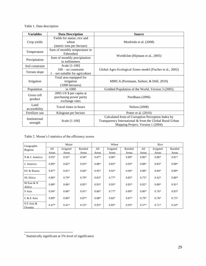
Data: We collected a variety of geo-spatial and national level data from several sources

(Table 1). Most of the geo-spatial data represent the 2000-2001 period. We use yield data for

maize, wheat and rice from Monfreda et al. (2008). Temperature and precipitation data were

taken from Worldclim (Hijmans et al., 2005) while soil fertility, terrain and slope constraints

were collected from Global Agro-Ecological Zones (GAEZ) model (Fischer et al., 2002). Socio-

economic variables used in this study include population, fertilizer use, irrigation, market access

and proxy variables for market influence and institutional strength. Population is based on the

Gridded Population of the World, Version 3 (2005). Fertilizer application rates is taken from

Potter et al. (2010) while area of irrigated land is collected from MIRCA (Portmann, Siebert, &

Döll, 2010). For market access, we use the global accessibility maps by Nelson (2008) which

measures the travel time in minutes to the nearest city with population of 50,000 or more for

each grid cell. A proxy for market influence is the Gross Cell Product (GCP) maps by Nordhaus

(2006). It is a spatially disaggregated measure of GDP and it is mostly based on detailed

economic data collected at the state or province level. To measure institutional strength, we

combine the national-level data on the ranges of Corruption Perception Index (CPI) by

Transparency International and the urban extent maps from the Global Rural-Urban Mapping

10

Project, Version 1 (2004). We assumed that, within a country, areas which have high

concentration of urban extents have stronger local institutions (high scores of Corruption

Perception) compared to areas which are more rural.

To separate rainfed from irrigated systems, we used the data on irrigation. Specifically

we assumed that irrigated (rainfed) systems have irrigated land areas which are greater than or

equal to (less than) 5000 hectares. In addition, we only focus on grid-cells which have more than

5% cropland area in order to exclude the effect of marginal lands using the Global Cropland and

Pasture Data maps by Ramankutty (2011).

III. Results and Discussions

Distribution of Efficiency Scores: The DEA scores are mapped to show the global

distribution of technical efficiency scores (Figures 1 to 9). From the maps, we see that areas

which have (low) high efficiencies are typically adjacent to each other together which suggests

spatial clustering. To formally quantify the degree of spatial clustering in the efficiency scores,

the Moran’s I test is conducted. The Moran’s I test provides a global measurement of spatial

autocorrelation among neighboring observations (Anselin, 1996). We implemented the Moran’s I

test on the efficiency scores for each geographic region. The results confirm that there is

clustering in the efficiency scores. Specifically, there is statistically significant and positive

spatial autocorrelation among the calculated efficiency scores (Table 2).

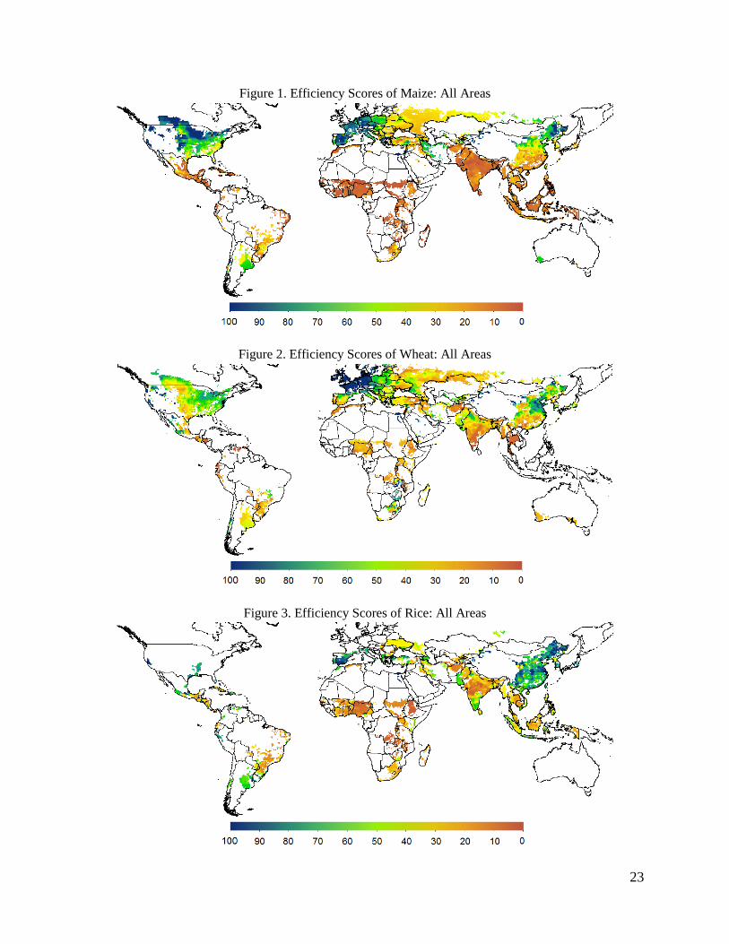
Scores which considers all areas are illustrated in Figures 1 to 3. Looking at maize, we

see that high scores (≥ 70%) are generally situated in North America, the European Union and in

the northeastern China. At a glance, we see that even at country-level, the distribution of

technical efficiency scores is quite heterogeneous. For example, scores in North America tend to

decline in areas situated near the eastern coast while scores in China are generally lower in the

11

southern than in the northern regions. Regions with low efficiency scores (≤ 30%) include

Central America, Sub-Saharan Africa (excluding South Africa), South and South East Asia. This

implies that these regions generally have large maize yield gaps due to technical inefficiency.

Efficiency scores in Russia, Latin America and Australia are generally less than in North

America but are still relatively high compared to the rest of the world. Unlike maize, efficiency

scores for wheat are more dispersed. High scores are generally located in the European Union,

North America and northeastern China. There are also some patches of technically efficient areas

in Africa and South Asia although these regions are still dominated by areas with low efficiency

scores. In Russia, areas near the Black Sea are more efficient compared to the rest of the country.

Looking at rice, we see that most efficient areas are located in China and in parts of the European

Union. Within South East Asia, Viet Nam and parts of Thailand and Indonesia have high

efficiency scores compared to other countries in the same region. Despite large concentration of

low efficiency scores, there are still some areas in India and Pakistan which have relatively high

scores. In Latin America, areas in Argentina are technically more efficient than those in Brazil.

Similar to the previous maps, rice efficiency scores in Africa are generally low which is

indicative of large yield gaps for this crop in this region.

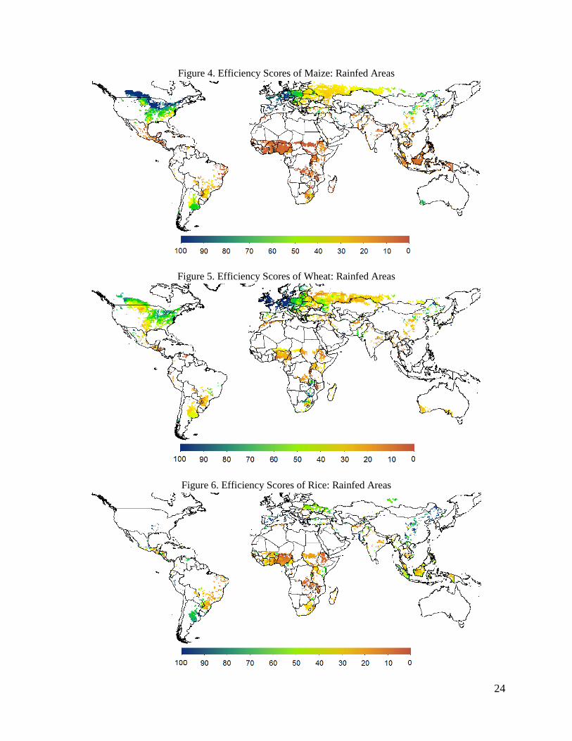
Efficiency scores generated for rainfed and irrigated areas are also mapped separately. In

general, the distribution of rainfed efficiency scores is quite similar to the case wherein all areas

are considered especially for maize and wheat (Figures 4 to 6). Rainfed maize and wheat areas

with high scores are again situated in North America and in the European Union. Central

America, Africa and South East Asia are generally dominated by low efficiency scores which

indicate significant yield gaps in rainfed maize and wheat for these regions. Relative to these

regions, Latin America and Russia generally have high scores. For rainfed rice, the improvement

12

in efficiency scores is more visible. We can see improvements in the efficiency scores in parts of

Argentina, Indonesia and Ukraine. This occurs because we are excluding the majority of

technically efficient areas (namely in northeast China) which in turn alters the technically

efficient set of observable rice yields.

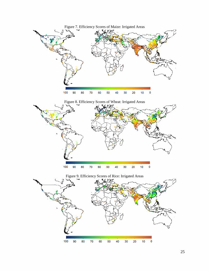
Similar to the case of rainfed areas, it is difficult to distinguish if there are changes in the

distribution of scores for irrigated areas versus all areas (Figures 7 to 9). The maps show that

most irrigated areas are located in South Asia, South East Asia and in China. For maize and

wheat, high scores are located in North America, the European Union and in northern China

while low efficiency scores are observed in South and South East Asia and in southern China.

For irrigated rice, high efficiency scores are again located in China and in parts of the European

Union while low efficiency scores are situated in South Asia and in parts of South East Asia.

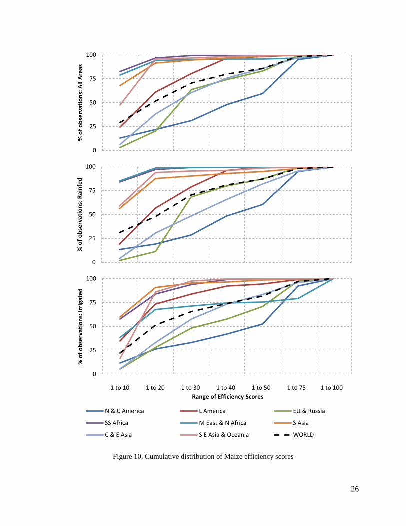
To clearly illustrate the changes in the distribution of technical efficiency scores for all

areas, rainfed areas and irrigated areas, we use cumulative histograms (Figures 10 to 12). We

plot the cumulative distribution of efficiency scores for 8 geographic regions. We also include

the global distribution as a baseline such that distributions to the left (right) of the global

distribution have relatively low (high) efficiency scores. Starting with maize, we see that the

global distribution does not change dramatically if we separate irrigated and rainfed areas

(Figure 10). Roughly 50% of global scores are in the interval [1, 20] for all cases which suggest

large yield gaps for this crop globally. Among the regions, scores in N & C America are always

on the right of these graphs which indicates that this region generally have high efficiency scores

compared to the rest of the world. It is interesting to note that there are some regions which show

changes in the distribution of scores when irrigated and rainfed areas are separated. For example,

in the case of all areas we see that the distribution for the EU & Russia and C & E Asia are close

13

to the global distribution. However, in the case of rainfed areas the distribution for C & E Asia

approaches that of N & C America. Under this case, more that 50% of rainfed areas in C & E

Asia have scores in the interval [1, 30] while it is higher for EU & Russia (75%). In the case of

irrigated areas, the distribution for EU & Russia is closer to N & C America while the

distribution for C & E Asia approaches the global distribution. Regions which have distributions

on the left of the global distribution include L America, SS Africa, M East & N Africa, S Asia

and SE Asia & Oceania. For these regions, greater than 75% of the all areas and rainfed areas

have efficiency scores in the interval [1, 30] which suggests that these regions are generally

inefficient compared to other world regions. There are some notable changes in the distribution

of scores under the case of irrigated area in particular for M East & N Africa and for L America.

For L America (M East & N Africa), the distribution shifts to the left (right) and moves away

from (closer to) the global distribution.

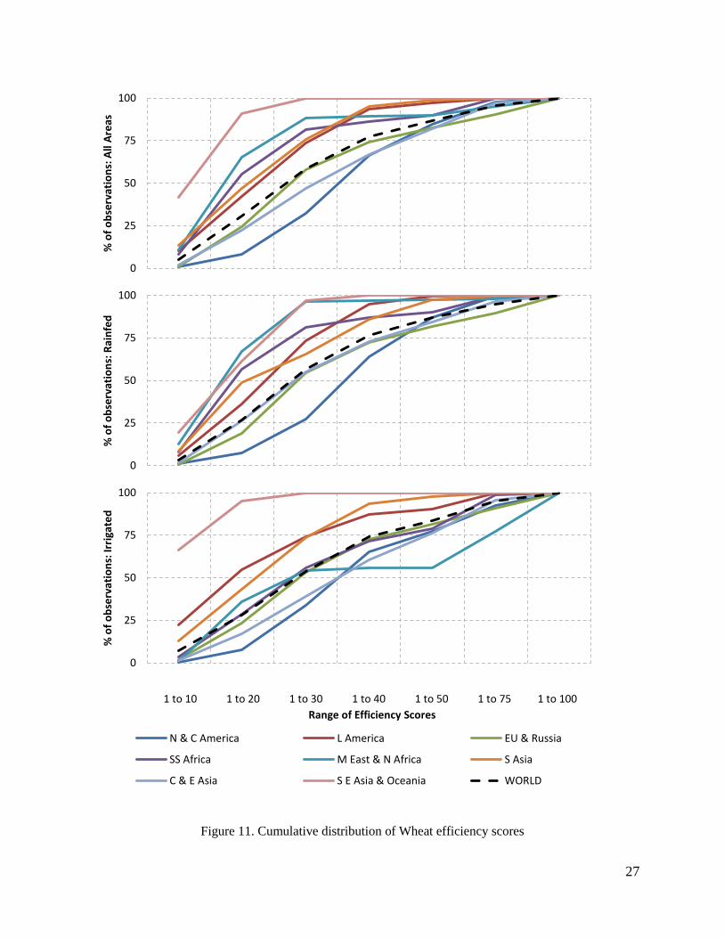
Compared to maize, the distribution of scores is less dispersed in the case of wheat

(Figure 11). Globally, around 25% of the efficiency scores are in the interval [1, 20] for all cases.

This implies that yield gaps in wheat are generally smaller relative to maize since more observed

wheat yields are closer to the technically efficient frontier. Similar to maize, we see that the

distribution of scores for N & C America is always on the right for these graphs. The distribution

of scores for EU & Russia is close to the global distribution for all cases. For C & E Asia, the

distribution is closer to N & C America in the case of all areas and irrigated areas while it is

close to EU & Russia in the case of rainfed areas. Distribution of efficiency scores for S Asia, L

America, and SE Asia & Oceania are always on the left of the global distribution. At least 75%

of the scores in these regions are within the interval [1, 30] which implies large inefficiencies in

wheat production for these regions. We can also observe this for M East & N Africa and SS

14

Africa in the case of all areas and for rainfed areas. However, we see that if we focus on irrigated

areas the distribution of scores in these regions shifts to the right. This is indicative that in these

regions irrigated areas have relatively high efficiency scores. In all cases, the distribution for SE

Asia & Oceania region is always on the right which suggest that wheat production in this region

is relatively inefficient compared to the rest of the world.

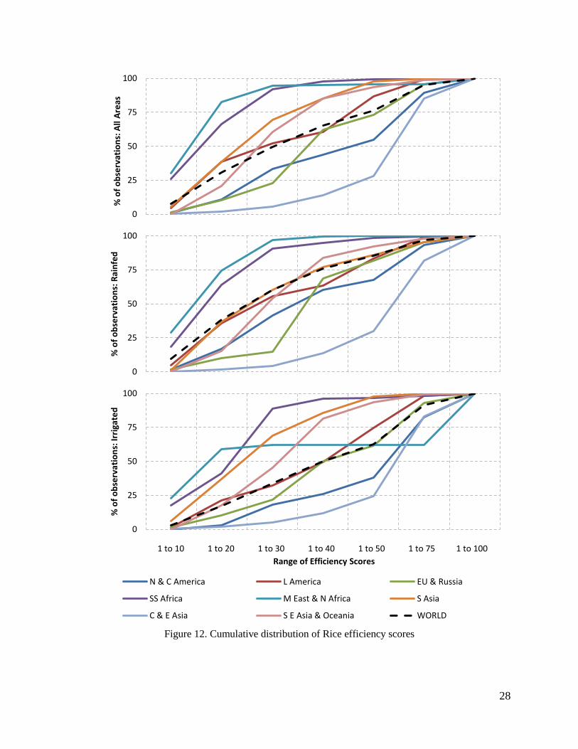
Efficiency scores for rice are more dispersed compared to maize and wheat (Figure 12).

More importantly, there are notable changes in the global distribution of scores between rainfed

and irrigated areas. If all areas are considered, roughly 50% of global scores are within the

interval [1, 30] while this increases to at least 60% if we look at rainfed areas. However, we see a

sizable decline in the case of irrigated areas (at least 30%). This implies greater efficiency in

observed irrigated rice yields compared to rainfed rice yields. The distribution for C & E Asia is

always on the right relative to other regions which suggests that rice production in this region is

quite efficient. Other regions on the right of the global distribution are N & C America and EU &

Russia. Looking at all areas, we see that regions to the left of the global distribution include M

East & N Africa, SS Africa, S Asia and SE Asia & Oceania. If we focus only at rainfed areas, S

Asia and SE Asia & Oceania shifts and moves closer to the global distribution while the

distributions for M East & N Africa and SS Africa remain unchanged. In the case of irrigated

areas, the distribution of scores for S Asia and for SE Asia & Oceania shifts to the left (becomes

more inefficient). In general, L America always follows the global distribution for rice.

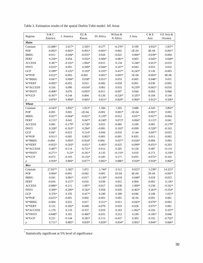
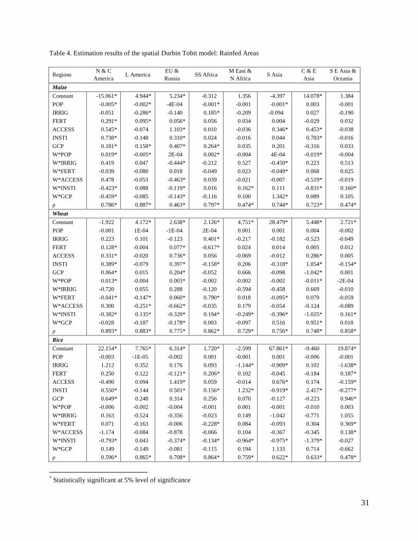
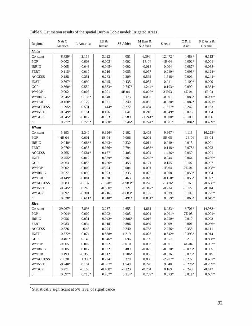
Estimation results: We estimate the SDT model for all areas, rainfed areas and irrigated

areas for each world regions (Tables 3 to 5). Explanatory variables for the calculated efficiency

scores include population (POP), fertilizer use (FERT), irrigation (IRRIG), market accessibility

(ACCESS) and proxy variables for market influence (GCP) and an index for institutional

15

strength (INSTI). Interpretation of the parameter estimates is not straight forward since the

spatial model takes into account the neighboring values of the efficiency scores and the

neighboring values of the explanatory variables. Given this, the marginal effect of an explanatory

variable in a grid-cell will not only affect the efficiency scores in that location but also the scores

in neighboring grid-cells.

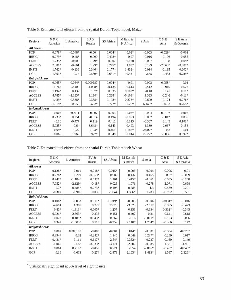
As discussed by LeSage and Fischer (2007), in models with spatial lags the changes in

the explanatory variables result in direct impacts in its own region as well as indirect impacts to

other regions. A formal method for calculating summary measures of the direct, indirect and total

impacts and their corresponding statistical measures of dispersion was introduced by Pace and

LeSage (2006). The authors defined the direct impact as the average impact of changes in a

variable within a region such that the feedback effects from neighboring regions are accounted

for. On the other hand, the total effect measures the average impact in a typical region if we

change a variable in all regions. This measure includes both the direct and indirect impacts.

Finally, the indirect effects which capture the spill-over effects across space can be calculated

from the difference between the total and direct impacts. The methods used to calculate these

summary impacts are in the Spatial Econometrics Toolbox by LeSage.

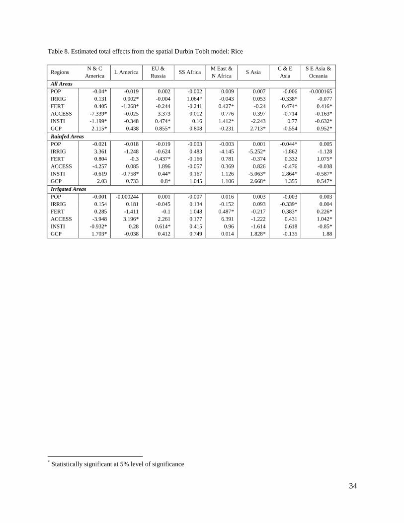
Estimates of total impacts are shown in Tables 6 to 8. We focus our discussion on

geographic regions which have large distribution of low efficiency scores based on the maps and

on the cumulative histograms (i.e. L America, SS Africa, SE Asia & Oceania, S Asia). Starting

with maize, we see that in L America population (-) and irrigation (+) are key factors affecting

the efficiency scores when all areas are considered. If we focus on rainfed areas, population,

irrigation and institutional strength have negative total impacts on efficiency. None of the socio-

economic variables have statistically significant total impacts on irrigated maize in this region.

16

Looking at all areas in SS Africa, we see that all variables except market access have statistically

significant and positive total effect on efficiency. In the case of rainfed areas, population, market

access, institutional strength and market influence have increasing total effects on efficiency

scores for this region. In S Asia, market influence has positive total impacts on efficiencies for

both rainfed and irrigated areas. For irrigated areas, institutional strength negatively affects

efficiency for this region. For SE Asia & Oceania for both all areas and rainfed areas, variables

which significantly affect the efficiency scores are fertilizer use (+), institutional strengths (+),

market influence (+) and market access (-). If we focus only on irrigated areas, fertilizer use and

institutional strength positively impacts efficiency.

In the case of wheat production, we see that in L America key drivers of efficiency scores

include fertilizer use (-), market access (-), and institutional strength (+) when all areas are

considered. The same factors plus market influence (-) are the main contributors to efficiency

under rainfed areas. Institutional strength (+) is the only statistically significant variable in the

case of irrigated areas in this region. In SS Africa, only population (-) is statistically significant

for both all areas and rainfed areas. Likewise, fertilizer use (+) is the only statistically significant

variable under the case of irrigated areas. In rainfed and irrigated areas in S Asia, main

contributors to efficiency scores are institutional strength (-) and market influence (+). Irrigation

also increases efficiency scores for irrigated areas in this region. In SE Asia & Oceania, only the

case of irrigated areas has statistically significant coefficients. For this region, the total effect on

efficiency of population and institutions are negative while it is positive for market influence.

For rice production, we see that most of the statistically significant variables are in L

America, S Asia and SE Asia & Oceania. If all areas are considered, irrigation contributes

positive to efficiency scores in L America while fertilizer use has an adverse impact. For rainfed

17

areas, institutional strength has an adverse effect while market access has a positive impact on

efficiency scores under irrigated areas. Efficiency scores for rice are positively affected by

market influence for all cases in S Asia. Variables which have negative impacts on scores for

rainfed areas in this region include institutional strength and irrigation. In SE Asia & Oceania,

key drivers of efficiency scores are fertilizer use (+) institutional strength (-). For both rainfed

and all areas, market influence contributes positively to efficiency scores in this region. Market

access also contributes to efficiency scores in the case of all lands (-) and irrigated lands (+).

The results discussed above show that the effects of the socio-economic variables on the

efficiency scores are not always consistent and will typically vary by geographic region, crop

type and scope of analysis (all areas, rainfed areas, irrigated areas). For example, the impact of

fertilizer in maize is consistently positive across all regions but for wheat and rice, its impacts are

mixed. In the case of rice, the total impact of irrigation on the efficiency scores are either zero or

negative for all areas, rainfed areas and irrigated areas. However, we can also see some general

trends. Most of the total impacts of socio-economic variables on efficiency scores are positive.

For example, across all crops and regions the total impact of irrigation, fertilizer use, institutional

strength and market influence are generally positive in the case of all areas. For rainfed areas,

fertilizer use and market influence are the key drivers of efficiency. These are also the drivers for

irrigated areas plus market access. If we look at each crop for all cases and regions, we see that

irrigation, fertilizer use, institutional strength and market influence are the important factors

affecting efficiency scores for maize. For wheat and rice, the main contributors to efficiencies are

fertilizer use and market influence. At regional level and for all crops and cases, we see that in L

America, institutional strength (+) and market access (-) generally have statistically significant

total impacts. For S Asia, market influence (+) and institutional strength (-) are the key drivers.

18

For SE Asia & Oceania, market influence (+) and fertilizer use (+) are important contributors to

efficiency. In the case of SS Africa, all except population generally have positive total impact on

efficiency. The results also indicate that by changing the coverage from all areas to either rainfed

or irrigated areas, we generally see that some variables become statistically significant while

some become insignificant. However, as long as the estimate is statistically significant in the

case of all areas we see that the signs of these estimates are generally consistent if we focus on

either rainfed or irrigated areas.

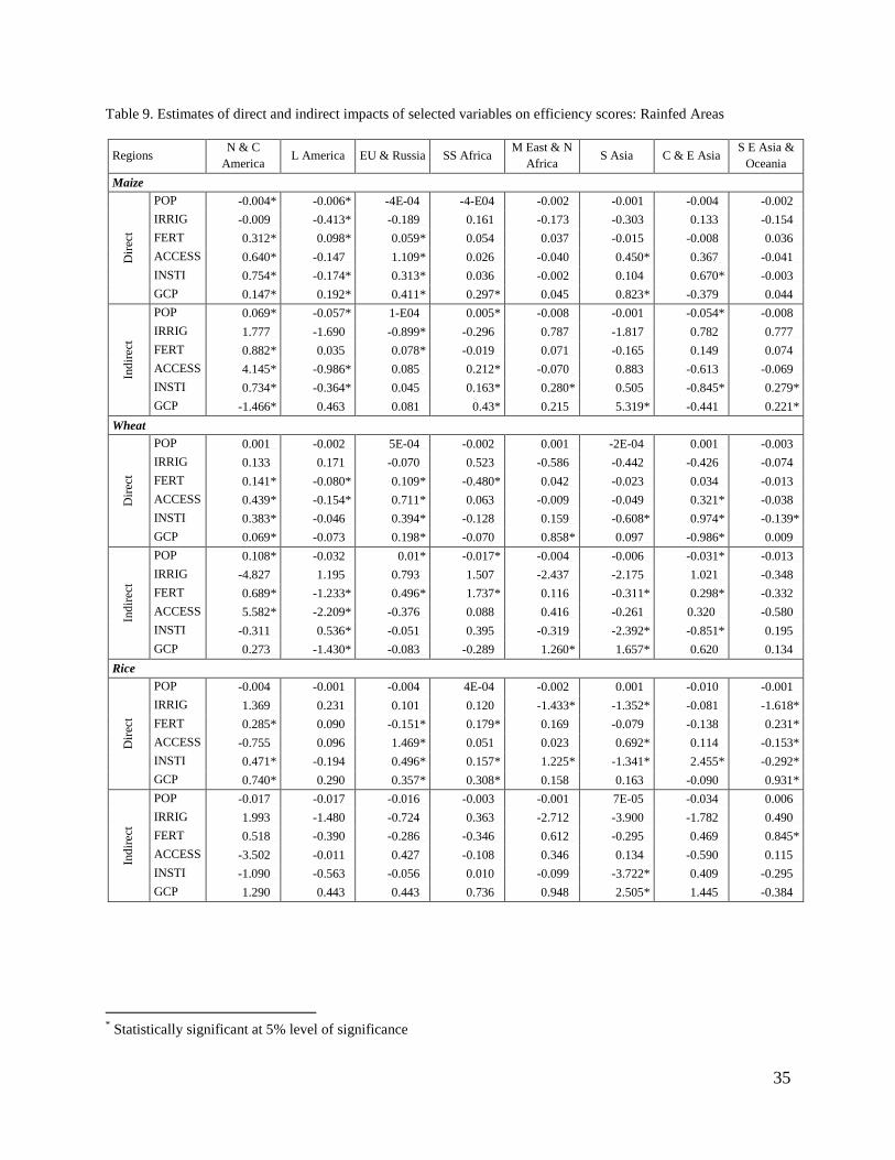
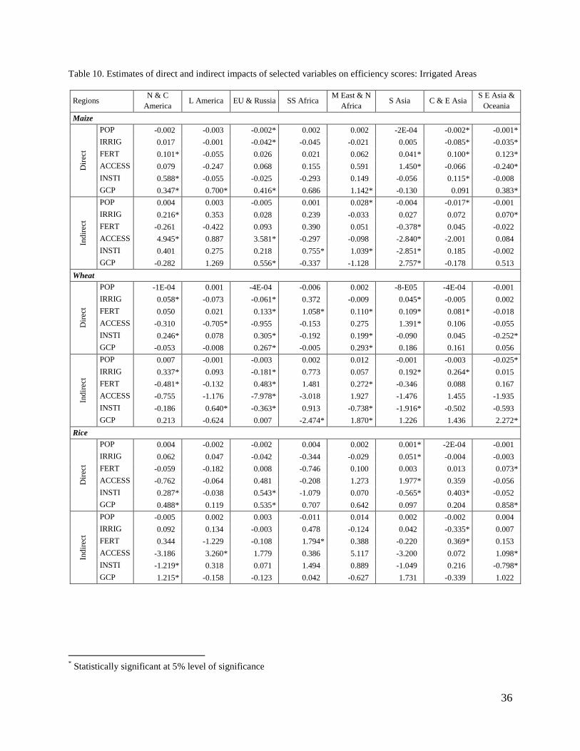
Finally, we explore the results of the model by isolating the direct and indirect effects of

the socio-economic variables on the efficiency scores (Tables 9 and 10). In general, these results

indicate that there are variables which do not have statistically significant total effect but have

statistically significant direct/indirect effects. For example, for rainfed maize in L America, we

see that irrigation (-) and market influence (+) become statistically significant in terms of its

direct effect. This is also true for the direct effects of fertilizer use (+), institutional strength (+)

and market influence (+) on efficiency scores of rainfed rice in SS Africa. In most cases, the

indirect effect is generally larger than direct effect. Examples of these include fertilizer use (-)

and market access (-) for rainfed wheat in L America and institutional strength (+) for rainfed

maize in S Asia. However, there are some instances wherein the signs of the direct and indirect

impacts are different. This is true in the case of fertilizer use and market access for rainfed maize

in S Asia and in irrigation in SE Asia & Oceania.

IV. Conclusion

In this study, we revisit global yield gap analysis by examining technical efficiencies in

global crop production and by relating these to selected socio-economic variables. To calculate

these efficiencies across the world, we apply data envelopment analysis on geo-spatial data on

19

crop yields and agro-climatic factors. This non-parametric approach allows us to generate scores

which represent how far the observed crop yields are from the technically efficient frontier given

its observed agro-climatic inputs. We then relate these efficiency scores to selected socio-

economic variables namely population, irrigation, fertilizer use, market access, institutional

strength and market influence. We apply spatial econometric techniques in our estimation to

account for the spatial correlation in the data and in the calculated scores. Specifically, we

estimated the spatial Durbin Tobit model using the methods outlined by LeSage (2000). The

results of the study show that the global distribution of calculated efficiency scores varies among

countries. More importantly, these scores vary within countries and this highlights the

importance of using spatial data on global yield gap analysis. We find that the effects of the

socio-economic variables on the efficiency scores are not always consistent and will typically

vary depending on region, crop and scope. However, we can also see some general trends. Most

of the total impacts of socio-economic variables on efficiency scores are positive. For example,

across all crops and regions the total impact of irrigation, fertilizer use, institutional strength and

market influence are generally positive if we look at all areas. By changing the coverage from all

areas to either rainfed or irrigated areas, we generally see that some variables become

statistically significant while some become insignificant. However, the signs of these estimates

are generally consistent if we examine all areas or if we limit our focus on rainfed or irrigated

areas. Given the spatial model, we can also explore the direct and indirect impacts of the socio-

economic variables on the efficiency scores. In some cases, there are variables which do not have

statistically significant total effect but have statistically significant direct/indirect effects. The

indirect effect is generally larger than direct effect which shows the importance of using spatial

econometric techniques to account for the spatial interaction in the data.

20

References:

Anselin, L. (1996). The Moran Scatterplot as an ESDA Tool to Assess Local Instability in Spatial Association.

Spatial Analytical Perspectives on GIS: GISDATA 4 (pp. 111–125). Taylor & Francis.

Anselin, Luc. (1988). Spatial Econometrics: Methods and Models. Dordrecht, The Netherlands: Kluwer Academic

Publishers.

Anselin, Luc. (2007). Spatial Econometrics. A Companion to Theoretical Econometrics (pp. 310–330). Blackwell

Publishing Ltd. Retrieved from http://dx.doi.org/10.1002/9780470996249.ch15

Banker, R. D., Charnes, A., & Cooper, W. W. (1984). Some Models for Estimating Technical and Scale

Inefficiencies in Data Envelopment Analysis. Management Science, 30(9), 1078–1092.

Battese, G. E., & Coelli, T. J. (1995). A model for technical inefficiency effects in a stochastic frontier production

function for panel data. Empirical Economics, 20, 325–332. doi:10.1007/BF01205442

Begum, I. A., Alam, M. J., Buysse, J., Frija, A., & Van Huylenbroeck, G. (2011). Contract farmer and poultry farm

efficiency in Bangladesh: a data envelopment analysis. Applied Economics, 44(28), 3737–3747.

doi:10.1080/00036846.2011.581216

Bravo-Ureta, B. E., Solís, D., Moreira López, V. H., Maripani, J. F., Thiam, A., & Rivas, T. (2006). Technical

efficiency in farming: a meta-regression analysis. Journal of Productivity Analysis, 27, 57–72.

doi:10.1007/s11123-006-0025-3

Bridging the rice yield gap in the Asia-Pacific region. (2000).RAP Publication. Food and Agriculture Organization

of the United Nations, Regional Office for Asia and the Pacific.

Center for International Earth Science Information Network, & Centro Internacional de Agricultura Tropical.

(2005). Gridded Population of the World, Version 3. Palisades, NY, USA: Socioeconomic Data and

Applications Center , Columbia University and Centro Internacional de Agricultura Tropical.

Center for International Earth Science Information Network, International Food Policy Research Institute, The

World Bank, & Centro Internacional de Agricultura Tropical. (2004). Global Rural-Urban Mapping

Project, Version 1. Palisades, NY: Socioeconomic Data and Applications Center, Columbia University:

Socioeconomic Data and Applications Center (SEDAC), Columbia University.

Charnes, A., Cooper, W. W., & Rhodes, E. (1978). Measuring the efficiency of decision making units. European

Journal of Operational Research, 2(6), 429–444. doi:10.1016/0377-2217(78)90138-8

Coelli, T. J. (1995). Recent Developments In Frontier Modelling And Efficiency Measurement. Australian Journal

of Agricultural Economics, Australian Journal of Agricultural Economics, 39(03). Retrieved from

http://ideas.repec.org/a/ags/ajaeau/22681.html

Coelli, T. J., Rao, D. S., O’Donnell, C. J., & Battese, G. E. (2005). An Introduction to Efficiency and Productivity

Analysis (2nd ed., Vols. 1-1). New York , USA: Springer.

De Datta, S. K. (1981). Principles and Practices of Rice Production. New York, USA: John Wiley & Sons.

Duwayri, M., Tran, D. V., & Nguyen, V. N. (2000). Reflections on Yield Gap in Rice Production: How to narrow

the gaps. In M. K. Papademetriou, F. J. Dent, & E. M. Herath (Eds.), Bridging the Rice Yield Gap in the

Asia-Pacific Region, RAP Publication (pp. 26–45). Bangkok, Thailand: Food and Agriculture Organization

of the United Nations, Regional Office for Asia and the Pacific.

Evans, L. T. (1993). Crop evolution, adaptation and yield. New York, NY, USA: Cambridge University Press.

Fageria, N. K. (1992). Maximizing Crop Yields. New York: Marcel Dekker.

Färe, R., Grosskopf, S., & Lovell, C. A. K. (1983). The Structure of Technical Efficiency. The Scandinavian Journal

of Economics, 85(2), 181–190. doi:10.2307/3439477

Farrell, M. J. (1957). The Measurement of Productive Efficiency. Journal of the Royal Statistical Society. Series A

(General), 120(3), 253–290. doi:10.2307/2343100

Fischer, G., Velthuizen, H. van, Shah, M., & Nachtergaele, F. (2002). Global Agro-ecological Assessment for

Agriculture in the 21st Century: Methodology and Results ( No. 02-02). Research Reports. International

Institute for Applied Systems Analysis.

Herdt, R. W. (1979). An Overview of the Constraints Project Results. Farm-Level Constraints to High Rice Yields in

Asia: 1974–1977 (pp. 395–421). Los Baños, Laguna, Philippines: International Rice Research Institute.

Hijmans, R. J., Cameron, S. E., Parra, J. L., Jones, P. G., & Jarvis, A. (2005). Very high resolution interpolated

climate surfaces for global land areas. International Journal of Climatology, 25(15), 1965–1978.

doi:10.1002/joc.1276

Hoff, A. (2007). Second stage DEA: Comparison of approaches for modelling the DEA score. European Journal of

Operational Research, 181(1), 425–435.

21

LeSage, J. P. (2000). Bayesian Estimation of Limited Dependent Variable Spatial Autoregressive Models.

Geographical Analysis, 32(1), 19–35. doi:10.1111/j.1538-4632.2000.tb00413.x

LeSage, J. P. (2010). Spatial Econometrics Toolbox for Matlab. Retrieved from http://www.spatial-

econometrics.com/

LeSage, J. P., & Fischer, M. M. (2007). Spatial Growth Regressions: Model Specification, Estimation and

Interpretation. SSRN eLibrary. Retrieved from http://papers.ssrn.com/sol3/papers.cfm?abstract_id=980965

Licker, R., Johnston, M., Foley, J. A., Barford, C., Kucharik, C. J., Monfreda, C., & Ramankutty, N. (2010). Mind

the gap: how do climate and agricultural management explain the “yield gap” of croplands around the

world? Global Ecology and Biogeography, 19(6), 769–782. doi:10.1111/j.1466-8238.2010.00563.x

Liu, Y., & Myers, R. (2008). Model selection in stochastic frontier analysis with an application to maize production

in Kenya. Journal of Productivity Analysis, 31, 33–46. doi:10.1007/s11123-008-0111-9

Lobell, D. B., Cassman, K. G., & Field, C. B. (2009). Crop Yield Gaps: Their Importance, Magnitudes, and Causes.

Annual Review of Environment and Resources, 34(1), 179–204.

doi:10.1146/annurev.environ.041008.093740

McDonald, J. (2009). Using least squares and tobit in second stage DEA efficiency analyses. European Journal of

Operational Research, 197(2), 792–798. doi:10.1016/j.ejor.2008.07.039

McMillen, D. P. (1992). Probit with Spatial Autocorrelation. Journal of Regional Science, 32(3), 335–348.

doi:10.1111/j.1467-9787.1992.tb00190.x

Monfreda, C., Ramankutty, N., & Foley, J. A. (2008). Farming the planet: 2. Geographic distribution of crop areas,

yields, physiological types, and net primary production in the year 2000. Global

Biogeochemical Cycles, 22, 19 PP. doi:200810.1029/2007GB002947

Murillo-Zamorano, L. R. (2004). Economic Efficiency and Frontier Techniques. Journal of Economic Surveys,

18(1), 33–77. doi:10.1111/j.1467-6419.2004.00215.x

Nelson, A. (2008). Estimated travel time to the nearest city of 50,000 or more people in year 2000. Ispra, Italy:

Global Environment Monitoring Unit - Joint Research Centre of the European Commission. Retrieved from

http://bioval.jrc.ec.europa.eu/products/gam/

Neumann, K., Verburg, P. H., Stehfest, E., & Müller, C. (2010). The yield gap of global grain production: A spatial

analysis. Agricultural Systems, 103(5), 316–326.

Nisrane, F., Berhane, G., Asrat, S., Getachew, G., Taffesse, A. S., & Hoddinott, J. (2011). Sources of Inefficiency

and Growth in Agricultural Output in Subsistence Agriculture: A Stochastic Frontier Analysis (ESSP II

Working Paper No. 19) (p. 55). Washington D.C., USA: Development Strategy and Governance Division,

International Food Policy Research Institute.

Nordhaus, W. D. (2006). Geography and macroeconomics: New data and new findings. Proceedings of the National

Academy of Sciences of the United States of America, 103(10), 3510 –3517. doi:10.1073/pnas.0509842103

Odeck, J. (2007). Measuring technical efficiency and productivity growth: a comparison of SFA and DEA on

Norwegian grain production data. Applied Economics, 39(20), 2617–2630.

doi:10.1080/00036840600722224

Pace, K. R., & LeSage, J. P. (2006). Interpreting Spatial Econometric Models. Presented at the Regional Science

Association International, North American Meetings, Toronto, CA.

Portmann, F. T., Siebert, S., & Döll, P. (2010). MIRCA2000—Global monthly irrigated and rainfed crop areas

around the year 2000: A new high-resolution data set for agricultural and hydrological

modeling. Global Biogeochemical Cycles, 24, 24 PP. doi:201010.1029/2008GB003435

Potter, P., Ramankutty, N., Bennett, E. M., & Donner, S. D. (2010). Characterizing the Spatial Patterns of Global

Fertilizer Application and Manure Production. Earth Interactions, 14(2), 1–22.

Ramalho, E., Ramalho, J., & Henriques, P. (2010). Fractional regression models for second stage DEA efficiency

analyses. Journal of Productivity Analysis, 34(3), 239–255. doi:10.1007/s11123-010-0184-0

Ramankutty, N. (2011). Global Cropland and Pasture Data: 1700-2007. Retrieved from

http://www.geog.mcgill.ca/~nramankutty/Datasets/Datasets.html

Sekhon, M., Mahal, A. K., Kaur, M., & Sidhu, M. (2010). Technical Efficiency in Crop Production: A Region-wise

Analysis. Agricultural Economics Research Review, 23(2), 367–374.

Singh, P., Aggarwal, P. K., Bahatia, V. S., Murty, M. R. V., Pala, M., Oweis, T., Benli, B., et al. (2009). Yield gap

analysis: Modeling of achievable yields at farm level. In S. Wani, J. Rockstrom, & T. Oweis (Eds.),

Rainfed agriculture: Unlocking the potential, Comprehensive Assessment of Water Management in

Agriculture Series (pp. 81–123). Oxfordshir, UK; Cambrige, MA, USA: CAB International.

22

Speelman, S., D’Haese, M., Buysse, J., & D’Haese, L. (2008). A measure for the efficiency of water use and its

determinants, a case study of small-scale irrigation schemes in North-West Province, South Africa.

Agricultural Systems, 98(1), 31–39. doi:10.1016/j.agsy.2008.03.006

Thiam, A., Bravo‐Ureta, B. E., & Rivas, T. E. (2005). Technical efficiency in developing country agriculture: a

meta‐analysis. Agricultural Economics, 25(2‐3), 235–243. doi:10.1111/j.1574-0862.2001.tb00204.x

van Ittersum, M. K., & Rabbinge, R. (1997). Concepts in production ecology for analysis and quantification of

agricultural input-output combinations. Field Crops Research, 52(3), 197–208. doi:16/S0378-

4290(97)00037-3

23

Figure 1. Efficiency Scores of Maize: All Areas

Figure 2. Efficiency Scores of Wheat: All Areas

Figure 3. Efficiency Scores of Rice: All Areas

24

Figure 4. Efficiency Scores of Maize: Rainfed Areas

Figure 5. Efficiency Scores of Wheat: Rainfed Areas

Figure 6. Efficiency Scores of Rice: Rainfed Areas

25

Figure 7. Efficiency Scores of Maize: Irrigated Areas

Figure 8. Efficiency Scores of Wheat: Irrigated Areas

Figure 9. Efficiency Scores of Rice: Irrigated Areas

26

Figure 10. Cumulative distribution of Maize efficiency scores

0

25

50

75

100

% o

f o

bse

rvat

ion

s: A

ll A

reas

0

25

50

75

100

% o

f o

bse

rvat

ion

s: R

ain

fed

0

25

50

75

100

% o

f o

bse

rvat

ion

s: Ir

riga

ted

1 to 10 1 to 20 1 to 30 1 to 40 1 to 50 1 to 75 1 to 100

Range of Efficiency Scores

0100

1 to 10 1 to 20 1 to 30 1 to 40 1 to 50 1 to 75 1 to 100

% o

f o

bse

rvat

io

ns

Range of Efficiency Scores: Global

N & C America L America EU & Russia

SS Africa M East & N Africa S Asia

C & E Asia S E Asia & Oceania WORLD

27

Figure 11. Cumulative distribution of Wheat efficiency scores

0

25

50

75

100%

of

ob

serv

atio

ns:

All

Are

as

0

25

50

75

100

% o

f o

bse

rvat

ion

s: R

ain

fed

0

25

50

75

100

% o

f o

bse

rvat

ion

s: Ir

riga

ted

1 to 10 1 to 20 1 to 30 1 to 40 1 to 50 1 to 75 1 to 100

Range of Efficiency Scores

0100

1 to 10 1 to 20 1 to 30 1 to 40 1 to 50 1 to 75 1 to 100

% o

f o

bse

rvat

io

ns

Range of Efficiency Scores: Global

N & C America L America EU & Russia

SS Africa M East & N Africa S Asia

C & E Asia S E Asia & Oceania WORLD

28

Figure 12. Cumulative distribution of Rice efficiency scores

0

25

50

75

100

% o

f o

bse

rvat

ion

s: A

ll A

reas

0

25

50

75

100

% o

f o

bse

rvat

ion

s: R

ain

fed

0

25

50

75

100

% o

f o

bse

rvat

ion

s: Ir

riga

ted

1 to 10 1 to 20 1 to 30 1 to 40 1 to 50 1 to 75 1 to 100

Range of Efficiency Scores

0100

1 to 10 1 to 20 1 to 30 1 to 40 1 to 50 1 to 75 1 to 100

% o

f o

bse

rvat

io

ns

Range of Efficiency Scores: Global

N & C America L America EU & Russia

SS Africa M East & N Africa S Asia

C & E Asia S E Asia & Oceania WORLD

29

Table 1. Data description

Variables Data Description Source

Crop yields

Yields for maize, rice and

wheat

(metric tons per hectare)

Monfreda et al. (2008)

Temperature Sum of monthly temperature in

Fahrenheit Worldclim (Hijmans et al., 2005)

Precipitation Sum of monthly precipitation

in millimeters

Soil constraint Scale [1-100]

100 – no constraint

1 – not suitable for agriculture

Global Agro-Ecological Zones model (Fischer et al., 2002) Terrain slope

Irrigation

Total area equipped for

irrigation

(1000 hectares)

MIRCA (Portmann, Siebert, & Döll, 2010)

Population in 1000 Gridded Population of the World, Version 3 (2005)

Gross cell

product

2005 US $ per capita at

purchasing power parity

exchange rates

Nordhaus (2006)

Land

accessibility Travel times in hours Nelson (2008)

Fertilizer use Kilogram per hectare Potter et al. (2010)

Institutional

strength Scale [1-100]

Calculated from of Corruption Perception Index by

Transparency International & from the Global Rural-Urban

Mapping Project, Version 1 (2004)

Table 2. Moran’s I statistics of the efficiency scores2

Geographic

Regions

Maize Wheat Rice

All

Areas

Irrigated

Areas

Rainfed

Areas

All

Areas

Irrigated

Areas

Rainfed

Areas

All

Areas

Irrigated

Areas

Rainfed

Areas

N & C America 0.93* 0.92* 0.94* 0.87* 0.86* 0.89* 0.86* 0.86* 0.81*

L America 0.89* 0.82* 0.93* 0.88* 0.83* 0.93* 0.88* 0.83* 0.89*

EU & Russia 0.87* 0.81* 0.84* 0.95* 0.92* 0.94* 0.88* 0.84* 0.89*

SS Africa 0.80* 0.79* 0.79* 0.83* 0.77* 0.85* 0.75* 0.42* 0.80*

M East & N

Africa 0.88* 0.86* 0.85* 0.93* 0.95* 0.85* 0.92* 0.89* 0.91*

S Asia 0.94* 0.86* 0.91* 0.86* 0.77* 0.89* 0.80* 0.76* 0.83*

C & E Asia 0.89* 0.80* 0.87* 0.88* 0.82* 0.87* 0.79* 0.78* 0.75*

S E Asia &

Oceania 0.47* 0.41* 0.55* 0.93* 0.85* 0.93* 0.57* 0.71* 0.54*

* Statistically significant at 5% level of significance

30

Table 3. Estimation results of the spatial Durbin Tobit model: All Areas3

Regions N & C

America L America

EU &

Russia SS Africa

M East &

N Africa S Asia

C & E

Asia

S E Asia &

Oceania

Maize

Constant -12.686* 2.617* 2.545* -0.277_ -6.370* 0.199_ 4.932* 1.837*

POP -0.002* -0.002* -0.001* -0.001* -0.002_ -2E-04_ 4E-04_ -0.001*

IRRIG -0.011_ -0.044* -0.035* 0.026_ -0.022_ 0.006* -0.039* -0.004_

FERT 0.250* 0.054_ 0.032* 0.084* 0.081* 0.003_ 0.043* 0.049*

ACCESS 0.387* -0.165* 1.064* -0.015_ 0.134_ 0.246* 0.413* -0.033_

INSTI 0.633* -0.091_ 0.209* 0.044* 0.247* -0.043_ 0.053_ 0.032_

GCP 0.189* 0.225* 0.193* 0.255* 0.437* -0.243* 0.126_ -0.003_

W*POP 0.012* -0.003_ -0.001 _ 0.001* 0.005* 1E-04_ -0.003* 9E-06_

W*IRRIG 0.047* 0.094* 0.038* 0.051* 0.033_ -0.005_ 0.048* 0.031_

W*FERT -0.092* -0.055_ 0.012_ -0.082_ -0.059_ -0.001_ -0.030_ -0.005_

W*ACCESS 0.556_ 0.096_ -0.634* 0.061_ 0.033_ -0.239* -0.665* -0.010_

W*INSTI -0.408* 0.076_ -0.093* -0.011_ -0.007_ 0.044_ -0.063_ 0.068_

W*GCP -0.367* -0.144_ 0.004_ -0.136_ -0.526* 0.335* -0.164_ 0.144_

ρ 0.870* 0.894* 0.665* 0.811* 0.829* 0.960* 0.912* 0.506*

Wheat

Constant -4.543* 3.892* 1.813* 1.584_ 1.503_ 3.688_ -4.543_ 3.892*

POP -0.001_ 0.001_ -1E-04_ -0.001_ 0.001* -1E-04_ -0.001* 0.001_

IRRIG 0.027* -0.064* -0.021* 0.129* -0.012_ 0.037* 0.027* -0.064_

FERT 0.115* 0.041_ 0.047* -0.249* 0.072* 0.094* 0.115* 0.041_

ACCESS 0.081_ -0.179* 0.728* 0.015_ -0.085_ 0.100_ 0.081_ -0.179*

INSTI 0.328* -0.163* 0.294* -0.081_ 0.102* -0.099_ 0.328* -0.163_

GCP 0.047_ -0.023_ 0.114* 0.044_ -0.016_ 0.144_ 0.047* -0.023_

W*POP 0.011* -0.002_ 0.002* -0.001_ -0.001_ 9-E05_ 0.011_ -0.002_

W*IRRIG -0.004 _ 0.093* -0.024* 0.004 _ 0.027* -0.026* -0.004_ 0.093_

W*FERT -0.055* -0.203* 0.031* 0.405* -0.025_ -0.099* -0.055* -0.203_

W*ACCESS 0.487* -0.114_ -0.751* -0.012_ 0.205_ -0.120_ 0.487_ -0.114_

W*INSTI -0.271* 0.23* -0.261* 0.135_ -0.133* 0.010_ -0.271_ 0.230*

W*GCP -0.072_ -0.103_ -0.110* -0.185_ 0.171_ -0.055_ -0.072* -0.103_

ρ 0.918* 0.860* 0.877* 0.865* 0.886* 0.929* 0.918* 0.860*

Rice

Constant 27.837* 5.582* 1.872_ 1.744* -3.511_ 8.023* 5.238* 14.325*

POP 0.004* -0.001_ -0.002_ 0.001_ 1E-04_ __4E-04_ 2E-04_ -0.001*

IRRIG 0.041_ 0.081* -0.017_ -0.130* -0.018_ 0.048* 0.018_ -0.022_

FERT -0.016_ 0.157* 0.010_ 0.039_ 0.051_ 0.004_ -0.002_ 0.136*

ACCESS -0.886* -0.111_ 1.097* -0.017_ -0.038_ 1.099* 0.238_ -0.161*

INSTI 0.509* -0.200* 0.542* 0.058_ 0.020_ -0.463* 0.303* -0.254*

GCP 0.376* 0.195_ 0.417* 0.249_ 0.399_ -0.046_ 0.249_ 1.015*

W*POP -0.015* -0.001_ 0.002_ -0.001_ 0.001_ 1E-04_ -0.001_ 0.001_

W*IRRIG -0.004_ 0.022_ 0.017_ 0.311* 0.011_ -0.043* -0.070* -0.003_

W*FERT 0.131_ -0.302* -0.049_ -0.079_ 0.019_ -0.028_ 0.075* 0.001_

W*ACCESS -1.178_ 0.110_ -0.557_ 0.019_ 0.163_ -1.062* -0.350_ 0.107*

W*INSTI -0.848* 0.161_ -0.466* -0.031_ 0.212_ 0.249_ -0.185* 0.046_

W*GCP 0.221_ -0.144_ -0.281* -0.113_ -0.437_ 0.303_ -0.332_ -0.702*

ρ 0.711* 0.885* 0.839* 0.829* 0.834* 0.902* 0.844* 0.666*

* Statistically significant at 5% level of significance

31

Table 4. Estimation results of the spatial Durbin Tobit model: Rainfed Areas4

Regions N & C

America L America

EU &

Russia SS Africa

M East &

N Africa S Asia

C & E

Asia

S E Asia &

Oceania

Maize

Constant -15.061* 4.944* 5.234* -0.312_ 1.356_ -4.397_ 14.078* 1.384_

POP -0.005* -0.002* -4E-04_ -0.001* -0.001_ -0.001* 0.003_ -0.001_

IRRIG -0.051_ -0.286* -0.140_ 0.185* -0.209_ -0.094 _ 0.027_ -0.190_

FERT 0.291* 0.095* 0.056* 0.056_ 0.034_ 0.004_ -0.029_ 0.032_

ACCESS 0.545* -0.074_ 1.103* 0.010_ -0.036_ 0.346* 0.453* -0.038_

INSTI 0.738* -0.148_ 0.310* 0.024_ -0.016_ 0.044_ 0.783* -0.016_

GCP 0.181* 0.158* 0.407* 0.264* 0.035_ 0.201_ -0.316_ 0.033_

W*POP 0.019* -0.005* 2E-04_ 0.002* -0.004_ 4E-04_ -0.019* -0.004_

W*IRRIG 0.419_ 0.047_ -0.444* -0.212_ 0.527_ -0.450* 0.223_ 0.513_

W*FERT -0.039_ -0.080_ 0.018_ -0.049_ 0.023_ -0.049* 0.068_ 0.025_

W*ACCESS 0.478_ -0.053_ -0.463* 0.039_ -0.021_ -0.007_ -0.519* -0.019_

W*INSTI -0.423* 0.088_ -0.119* 0.016_ 0.162* 0.111_ -0.831* 0.160*

W*GCP -0.459* -0.085_ -0.143* -0.116_ 0.100_ 1.342* 0.089_ 0.105_

ρ 0.786* 0.887* 0.463* 0.797* 0.474* 0.744* 0.723* 0.474*

Wheat

Constant -1.922_ 4.172* 2.638* 2.126* 4.751* 28.479* 5.448* 2.721*

POP -0.001_ 1E-04_ -1E-04_ 2E-04_ 0.001_ 0.001_ 0.004_ -0.002_

IRRIG 0.223_ 0.101_ -0.123_ 0.401* -0.217_ -0.182_ -0.523_ -0.049_

FERT 0.128* -0.004_ 0.077* -0.617* 0.024_ 0.014_ 0.005_ 0.012_

ACCESS 0.331* -0.020_ 0.736* 0.056_ -0.069_ -0.012_ 0.286* 0.005_

INSTI 0.389* -0.079_ 0.397* -0.158* 0.206_ -0.318* 1.054* -0.154*

GCP 0.064* 0.015_ 0.204* -0.052_ 0.666_ -0.098_ -1.042* 0.001_

W*POP 0.013* -0.004_ 0.003* -0.002_ -0.002_ -0.002_ -0.011* -2E-04_

W*IRRIG -0.720_ 0.055_ 0.288_ -0.120_ -0.594_ -0.458_ 0.669_ -0.010_

W*FERT -0.041* -0.147* 0.060* 0.790* 0.018_ -0.095* 0.079_ -0.059_

W*ACCESS 0.300_ -0.251* -0.662* -0.035_ 0.179_ -0.054_ -0.124_ -0.089_

W*INSTI -0.382* 0.135* -0.320* 0.194* -0.249* -0.396* -1.025* 0.161*

W*GCP -0.028_ -0.187_ -0.178* 0.003_ -0.097_ 0.516_ 0.951* 0.018_

ρ 0.893* 0.883* 0.775* 0.862* 0.729* 0.756* 0.748* 0.858*

Rice

Constant 22.154* 7.765* 6.314* 1.720* -2.599_ 67.861* -9.460_ 19.874*

POP -0.003_ -1E-05_ -0.002_ 0.001_ -0.001_ 0.001_ -0.006_ -0.001_

IRRIG 1.212_ 0.352_ 0.176_ 0.093_ -1.144* -0.909* 0.102_ -1.638*

FERT 0.250_ 0.122_ -0.121* 0.206* 0.102_ -0.045_ -0.184_ 0.187*

ACCESS -0.490_ 0.094_ 1.419* 0.059_ -0.014_ 0.676* 0.174_ -0.159*

INSTI 0.550* -0.144_ 0.501* 0.156* 1.232* -0.919* 2.417* -0.277*

GCP 0.649* 0.248_ 0.314_ 0.256_ 0.070_ -0.127_ -0.223_ 0.946*

W*POP -0.006_ -0.002_ -0.004_ -0.001_ 0.001_ -0.001_ -0.010_ 0.003_

W*IRRIG 0.163_ -0.524_ -0.356_ -0.023_ 0.149_ -1.042_ -0.771_ 1.055_

W*FERT 0.071_ -0.163_ -0.006_ -0.228* 0.084_ -0.093_ 0.304_ 0.369*

W*ACCESS -1.174_ -0.084_ -0.878_ -0.066_ 0.104_ -0.367_ -0.345_ 0.138*

W*INSTI -0.793* 0.043_ -0.374* -0.134* -0.964* -0.975* -1.379* -0.027_

W*GCP 0.149_ -0.149_ -0.081_ -0.115_ 0.194_ 1.133_ 0.714_ -0.662_

ρ 0.596* 0.865* 0.708* 0.864* 0.759* 0.622* 0.633* 0.478*

* Statistically significant at 5% level of significance

32

Table 5. Estimation results of the spatial Durbin Tobit model: Irrigated Areas5

Regions N & C

America L America

EU &

Russia SS Africa

M East &

N Africa S Asia

C & E

Asia

S E Asia &

Oceania

Maize

Constant -8.739* -2.115_ 3.022_ -4.051_ -6.396 _ 12.472* 4.488* 6.112*

POP -0.002_ -0.003_ -0.002* 0.002_ -1E-04_ -1E-04_ -0.002* -0.001*

IRRIG 0.005_ -0.043_ -0.045* -0.092_ -0.018_ 0.004_ -0.087* -0.038*

FERT 0.115* -0.010_ 0.016_ -0.055_ 0.057_ 0.049* 0.098* 0.124*

ACCESS -0.185_ -0.351_ -0.283_ 0.209_ 0.592_ 1.518* 0.006_ -0.244*

INSTI 0.567* -0.090_ -0.045_ -0.435_ 0.052_ 0.011_ 0.109* -0.009_

GCP 0.360* 0.550_ 0.363* 0.747* 1.244* -0.193* 0.099_ 0.364*

W*POP 0.002_ 0.003_ -0.001_ -4E-04 _ 0.007* -3-E03_ -4E-04_ 1E-04_

W*IRRIG 0.045* 0.138* 0.040_ 0.173_ 0.005_ -0.001_ 0.086* 0.056*

W*FERT -0.150* -0.122_ 0.021_ 0.240_ -0.032_ -0.088* -0.082* -0.071*

W*ACCESS 1.295* 0.531_ 1.444* -0.272_ -0.484_ -1.677* -0.242_ 0.163_

W*INSTI -0.349* 0.151_ 0.106_ 0.641_ 0.210_ -0.349* -0.075_ 0.004_

W*GCP -0.345* -0.012_ -0.053_ -0.589_ -1.241* 0.500* -0.109_ 0.106_

ρ 0.777* 0.723* 0.680* 0.546* 0.774* 0.881* 0.884* 0.469*

Wheat

Constant 5.193_ 2.340_ 9.126* 2.182_ 2.403_ 9.867* 4.118_ 16.223*

POP -4E-04_ 0.001_ -1E-04_ -0.006_ 0.001_ -5E-05_ -2E-04 -2E-04_

IRRIG 0.040* -0.083* -0.043* 0.230_ -0.014_ 0.040* -0.015_ 0.001_

FERT 0.076* 0.035_ 0.086* 0.794_ 0.085* 0.118* 0.078* -0.023_

ACCESS -0.265_ -0.581* -0.167_ 0.405_ 0.094_ 1.426* 0.050_ -0.001_

INSTI 0.255* 0.012_ 0.339* -0.361_ 0.268* -0.044_ 0.064_ -0.236*

GCP -0.063_ 0.058_ 0.266* 0.453_ 0.121_ 0.155_ 0.107_ -0.007_

W*POP 0.002_ -0.002_ -4E-04_ 0.004_ 0.001_ -1E-04_ -2E-04_ -0.008*

W*IRRIG 0.027_ 0.092_ -0.003_ 0.335_ 0.022_ -0.008_ 0.050* 0.004_

W*FERT -0.149* -0.081_ 0.030_ 0.463_ -0.029_ -0.150* -0.055* 0.072_

W*ACCESS 0.083_ -0.137_ -1.528* -1.983* 0.228_ -1.436* 0.160_ -0.658*

W*INSTI -0.245* 0.260_ -0.350* 0.721_ -0.347* -0.234_ -0.127_ -0.044_

W*GCP 0.092_ -0.301_ -0.216_ -1.683* 0.197_ 0.039_ 0.109_ 0.777*

ρ 0.828* 0.611* 0.810* 0.491* 0.851* 0.859* 0.863* 0.645*

Rice

Constant 29.967* 7.898_ 3.237_ 0.655_ -4.661_ 8.983* 6.701* 14.983*

POP 0.004* -0.002_ -0.002_ 0.005_ 0.001_ 0.001* 7E-05_ -0.001*

IRRIG 0.056_ 0.031_ -0.042* -0.386* -0.016_ 0.050* 0.010_ -0.003_

FERT -0.083_ -0.034_ 0.018_ -0.896_ 0.059_ 0.009_ -0.001_ 0.066*

ACCESS -0.526_ -0.45_ 0.294_ -0.240_ 0.738_ 2.056* 0.355_ -0.111_

INSTI 0.372* -0.074_ 0.538* -1.219_ -0.023_ -0.542* 0.393* -0.014_

GCP 0.401* 0.143_ 0.546* 0.696_ 0.709_ 0.057_ 0.218_ 0.808*

W*POP -0.005_ 0.002_ 0.002_ -0.010_ 0.003_ -0.001_ 4E-04_ 0.002*

W*IRRIG 0.005_ 0.017_ 0.032_ 0.489_ -0.022_ -0.038* -0.073* 0.005_

W*FERT 0.193_ -0.355_ -0.042_ 1.706* 0.065_ -0.036_ 0.073* 0.015_

W*ACCESS -1.030_ 1.336* 0.224_ 0.370_ 0.888_ -2.207* -0.272_ 0.481*

W*INSTI -0.740* 0.154_ -0.397* 1.540_ 0.270_ 0.340_ -0.276* -0.289*

W*GCP 0.271_ -0.156_ -0.450* -0.123_ -0.704_ 0.169_ -0.243_ -0.143_

ρ 0.597* 0.716* 0.767* 0.214* 0.739* 0.873* 0.811* 0.637*

* Statistically significant at 5% level of significance

33

Table 6. Estimated total effects from the spatial Durbin Tobit model: Maize6

Regions N & C

America L America

EU &

Russia SS Africa

M East &

N Africa S Asia

C & E

Asia

S E Asia

& Oceania

All Areas

POP 0.078* -0.048* -0.004 0.004* 0.02* -0.003 -0.029* -0.001

IRRIG 0.279* 0.48* 0.009 0.408* 0.07 0.016 0.106 0.055

FERT 1.235* -0.006 0.129* 0.007 0.128 0.037 0.158 0.09*

ACCESS 7.381* -0.661 1.29* 0.245* 1.007 0.199 -2.868* -0.087*

INSTI 1.762* -0.139 0.346* 0.177* 1.432* 0.014 -0.115 0.202*

GCP -1.391* 0.76 0.589* 0.631* -0.531 2.35 -0.433 0.289*

Rainfed Areas

POP 0.065* -0.064* -0.000287 0.004* -0.01 -0.002 -0.058* -0.01

IRRIG 1.768 -2.103 -1.088* -0.135 0.614 -2.12 0.915 0.623

FERT 1.194* 0.132 0.137* 0.035 0.108* -0.18 0.141 0.11*

ACCESS 4.785* -1.133* 1.194* 0.238* -0.109* 1.333 -0.246 -0.11*

INSTI 1.489* -0.538* 0.358* 0.198* 0.278* 0.609 -0.174 0.276*

GCP -1.319* 0.656 0.492* 0.727* 0.26* 6.143* -0.82 0.265*

Irrigated Areas

POP 0.002 0.00011 -0.007 0.003 0.03* -0.004 -0.019* -0.002

IRRIG 0.233* 0.351 -0.014 0.194 -0.053 0.032 -0.012 0.035

FERT -0.16 -0.477 0.119 0.412 0.113 -0.337 0.145 0.101*

ACCESS 5.025* 0.64 3.648* -0.143 0.493 -1.389 -2.067 -0.156

INSTI 0.99* 0.22 0.194* 0.461 1.187* -2.907* 0.3 -0.01

GCP 0.065 1.969 0.972* 0.349 0.014 2.627* -0.086 0.897*

Table 7. Estimated total effects from the spatial Durbin Tobit model: Wheat

Regions N & C

America L America

EU &

Russia SS Africa

M East &

N Africa S Asia

C & E

Asia

S E Asia

& Oceania

All Areas

POP 0.128* -0.011 0.018* -0.015* 0.005 -0.004 -0.006 -0.01

IRRIG 0.278* 0.209 -0.363* 0.982 0.137 0.165 0.5* -0.059

FERT 0.747* -1.184* 0.637* 1.161 0.415* -0.061 0.055 -0.258

ACCESS 7.052* -2.129* -0.187 0.023 1.071 -0.278 2.071 -0.658

INSTI 0.7* 0.488* 0.273* 0.408 -0.285 -1.3 0.439 -0.201

GCP -0.307 -0.916 0.035 -1.044 1.396* 1.283 -0.192 0.561

Rainfed Areas

POP 0.108* -0.033 0.011* -0.019* -0.003 -0.006 -0.031* -0.016

IRRIG -4.694 1.365 0.723 2.029 -3.023 -2.617 0.595 -0.423

FERT 0.83* -1.313* 0.605* 1.257 0.158 -0.334 0.332* -0.345

ACCESS 6.021* -2.363* 0.335 0.151 0.407 -0.31 0.641 -0.618

INSTI 0.072 0.489* 0.343* 0.267 -0.16 -3.001* 0.123 0.056

GCP 0.342 -1.503* 0.115 -0.359 2.118* 1.754* -0.366 0.142

Irrigated Areas

POP 0.007 0.000187 -0.003 -0.004 0.014* -0.001 -0.004 -0.026*

IRRIG 0.394* 0.02 -0.242* 1.145 0.049 0.237* 0.259 0.017

FERT -0.431* -0.111 0.617* 2.54* 0.382* -0.237 0.169 0.149

ACCESS -1.065 -1.88 -8.933* -3.171 2.202 -0.085 1.561 -1.991

INSTI 0.061 0.718* -0.058 0.721 -0.54 -2.006* -0.457 -0.845*

GCP 0.16 -0.633 0.274 -2.479 2.163* 1.413* 1.597 2.328*

* Statistically significant at 5% level of significance

34

Table 8. Estimated total effects from the spatial Durbin Tobit model: Rice7

Regions N & C

America L America

EU &

Russia SS Africa

M East &

N Africa S Asia

C & E

Asia

S E Asia &

Oceania

All Areas

POP -0.04* -0.019 0.002 -0.002 0.009 0.007 -0.006 -0.000165

IRRIG 0.131 0.902* -0.004 1.064* -0.043 0.053 -0.338* -0.077

FERT 0.405 -1.268* -0.244 -0.241 0.427* -0.24 0.474* 0.416*

ACCESS -7.339* -0.025 3.373 0.012 0.776 0.397 -0.714 -0.163*

INSTI -1.199* -0.348 0.474* 0.16 1.412* -2.243 0.77 -0.632*

GCP 2.115* 0.438 0.855* 0.808 -0.231 2.713* -0.554 0.952*

Rainfed Areas

POP -0.021 -0.018 -0.019 -0.003 -0.003 0.001 -0.044* 0.005

IRRIG 3.361 -1.248 -0.624 0.483 -4.145 -5.252* -1.862 -1.128

FERT 0.804 -0.3 -0.437* -0.166 0.781 -0.374 0.332 1.075*

ACCESS -4.257 0.085 1.896 -0.057 0.369 0.826 -0.476 -0.038

INSTI -0.619 -0.758* 0.44* 0.167 1.126 -5.063* 2.864* -0.587*

GCP 2.03 0.733 0.8* 1.045 1.106 2.668* 1.355 0.547*

Irrigated Areas

POP -0.001 -0.000244 0.001 -0.007 0.016 0.003 -0.003 0.003

IRRIG 0.154 0.181 -0.045 0.134 -0.152 0.093 -0.339* 0.004

FERT 0.285 -1.411 -0.1 1.048 0.487* -0.217 0.383* 0.226*

ACCESS -3.948 3.196* 2.261 0.177 6.391 -1.222 0.431 1.042*

INSTI -0.932* 0.28 0.614* 0.415 0.96 -1.614 0.618 -0.85*

GCP 1.703* -0.038 0.412 0.749 0.014 1.828* -0.135 1.88

* Statistically significant at 5% level of significance

35

Table 9. Estimates of direct and indirect impacts of selected variables on efficiency scores: Rainfed Areas8

Regions N & C

America L America EU & Russia SS Africa

M East & N

Africa S Asia C & E Asia

S E Asia &

Oceania

Maize

Dir

ect

POP -0.004* -0.006* -4E-04_ -4-E04_ -0.002_ -0.001_ -0.004_ -0.002_

IRRIG -0.009_ -0.413* -0.189_ 0.161_ -0.173_ -0.303_ 0.133_ -0.154_

FERT 0.312* 0.098* 0.059* 0.054_ 0.037_ -0.015_ -0.008_ 0.036_

ACCESS 0.640* -0.147_ 1.109* 0.026_ -0.040_ 0.450* 0.367_ -0.041_

INSTI 0.754* -0.174* 0.313* 0.036_ -0.002_ 0.104_ 0.670* -0.003_

GCP 0.147* 0.192* 0.411* 0.297* 0.045_ 0.823* -0.379_ 0.044_

Ind

irec

t

POP 0.069* -0.057* 1-E04_ 0.005* -0.008_ -0.001_ -0.054* -0.008_

IRRIG 1.777_ -1.690_ -0.899* -0.296_ 0.787_ -1.817_ 0.782_ 0.777_

FERT 0.882* 0.035_ 0.078* -0.019_ 0.071_ -0.165_ 0.149_ 0.074_

ACCESS 4.145* -0.986* 0.085_ 0.212* -0.070_ 0.883_ -0.613_ -0.069_

INSTI 0.734* -0.364* 0.045_ 0.163* 0.280* 0.505_ -0.845* 0.279*

GCP -1.466* 0.463_ 0.081_ 0.43* 0.215_ 5.319* -0.441_ 0.221*

Wheat

Dir

ect

POP 0.001_ -0.002_ 5E-04_ -0.002_ 0.001_ -2E-04_ 0.001_ -0.003_

IRRIG 0.133_ 0.171_ -0.070_ 0.523_ -0.586_ -0.442_ -0.426_ -0.074_

FERT 0.141* -0.080* 0.109* -0.480* 0.042_ -0.023_ 0.034_ -0.013_

ACCESS 0.439* -0.154* 0.711* 0.063_ -0.009_ -0.049_ 0.321* -0.038_

INSTI 0.383* -0.046_ 0.394* -0.128_ 0.159_ -0.608* 0.974* -0.139*

GCP 0.069* -0.073_ 0.198* -0.070_ 0.858* 0.097_ -0.986* 0.009_

Ind

irec

t

POP 0.108* -0.032_ 0.01* -0.017* -0.004_ -0.006_ -0.031* -0.013_

IRRIG -4.827_ 1.195_ 0.793_ 1.507_ -2.437_ -2.175_ 1.021_ -0.348_

FERT 0.689* -1.233* 0.496* 1.737* 0.116_ -0.311* 0.298* -0.332_

ACCESS 5.582* -2.209* -0.376_ 0.088_ 0.416_ -0.261_ 0.320 _ -0.580_

INSTI -0.311_ 0.536* -0.051_ 0.395_ -0.319_ -2.392* -0.851* 0.195_

GCP 0.273_ -1.430* -0.083_ -0.289_ 1.260* 1.657* 0.620_ 0.134_

Rice

Dir

ect

POP -0.004_ -0.001_ -0.004_ 4E-04_ -0.002_ 0.001_ -0.010_ -0.001_

IRRIG 1.369_ 0.231_ 0.101_ 0.120_ -1.433* -1.352* -0.081_ -1.618*

FERT 0.285* 0.090_ -0.151* 0.179* 0.169_ -0.079_ -0.138_ 0.231*

ACCESS -0.755_ 0.096_ 1.469* 0.051_ 0.023_ 0.692* 0.114_ -0.153*

INSTI 0.471* -0.194_ 0.496* 0.157* 1.225* -1.341* 2.455* -0.292*

GCP 0.740* 0.290_ 0.357* 0.308* 0.158_ 0.163_ -0.090_ 0.931*

Ind

irec

t

POP -0.017_ -0.017_ -0.016_ -0.003_ -0.001_ 7E-05_ -0.034_ 0.006_

IRRIG 1.993_ -1.480_ -0.724_ 0.363_ -2.712_ -3.900_ -1.782_ 0.490_

FERT 0.518_ -0.390_ -0.286_ -0.346_ 0.612_ -0.295_ 0.469_ 0.845*

ACCESS -3.502_ -0.011_ 0.427_ -0.108_ 0.346_ 0.134_ -0.590_ 0.115_

INSTI -1.090_ -0.563_ -0.056_ 0.010_ -0.099_ -3.722* 0.409_ -0.295_

GCP 1.290_ 0.443_ 0.443_ 0.736_ 0.948_ 2.505* 1.445_ -0.384_

* Statistically significant at 5% level of significance

36

Table 10. Estimates of direct and indirect impacts of selected variables on efficiency scores: Irrigated Areas 9

Regions N & C

America L America EU & Russia SS Africa

M East & N

Africa S Asia C & E Asia

S E Asia &

Oceania

Maize

Dir

ect

POP -0.002_ -0.003_ -0.002* 0.002_ 0.002_ -2E-04_ -0.002* -0.001*

IRRIG 0.017_ -0.001_ -0.042* -0.045_ -0.021_ 0.005_ -0.085* -0.035*

FERT 0.101* -0.055_ 0.026_ 0.021_ 0.062_ 0.041* 0.100* 0.123*

ACCESS 0.079_ -0.247_ 0.068_ 0.155_ 0.591_ 1.450* -0.066_ -0.240*

INSTI 0.588* -0.055_ -0.025_ -0.293_ 0.149_ -0.056_ 0.115* -0.008_

GCP 0.347* 0.700* 0.416* 0.686_ 1.142* -0.130_ 0.091 0.383*

Ind

irec

t

POP 0.004_ 0.003_ -0.005_ 0.001_ 0.028* -0.004_ -0.017* -0.001_

IRRIG 0.216* 0.353_ 0.028_ 0.239_ -0.033_ 0.027_ 0.072_ 0.070*

FERT -0.261_ -0.422_ 0.093_ 0.390_ 0.051_ -0.378* 0.045_ -0.022_

ACCESS 4.945* 0.887_ 3.581* -0.297_ -0.098_ -2.840* -2.001_ 0.084_

INSTI 0.401_ 0.275_ 0.218_ 0.755* 1.039* -2.851* 0.185_ -0.002_

GCP -0.282_ 1.269_ 0.556* -0.337_ -1.128_ 2.757* -0.178_ 0.513_

Wheat

Dir

ect

POP -1E-04_ 0.001_ -4E-04_ -0.006_ 0.002_ -8-E05_ -4E-04_ -0.001_

IRRIG 0.058* -0.073_ -0.061* 0.372_ -0.009_ 0.045* -0.005_ 0.002_

FERT 0.050_ 0.021_ 0.133* 1.058* 0.110* 0.109* 0.081* -0.018_

ACCESS -0.310_ -0.705* -0.955_ -0.153_ 0.275_ 1.391* 0.106_ -0.055_

INSTI 0.246* 0.078_ 0.305* -0.192_ 0.199* -0.090_ 0.045_ -0.252*

GCP -0.053_ -0.008_ 0.267* -0.005_ 0.293* 0.186_ 0.161_ 0.056_

Ind

irec

t

POP 0.007_ -0.001_ -0.003_ 0.002_ 0.012_ -0.001_ -0.003_ -0.025*

IRRIG 0.337* 0.093_ -0.181* 0.773_ 0.057_ 0.192* 0.264* 0.015_

FERT -0.481* -0.132_ 0.483* 1.481_ 0.272* -0.346_ 0.088_ 0.167_

ACCESS -0.755_ -1.176_ -7.978* -3.018_ 1.927_ -1.476_ 1.455_ -1.935_

INSTI -0.186_ 0.640* -0.363* 0.913_ -0.738* -1.916* -0.502_ -0.593_

GCP 0.213_ -0.624_ 0.007_ -2.474* 1.870* 1.226_ 1.436_ 2.272*

Rice

Dir

ect

POP 0.004_ -0.002_ -0.002_ 0.004_ 0.002_ 0.001* -2E-04_ -0.001_

IRRIG 0.062_ 0.047_ -0.042_ -0.344_ -0.029_ 0.051* -0.004_ -0.003_

FERT -0.059_ -0.182_ 0.008_ -0.746_ 0.100_ 0.003_ 0.013_ 0.073*

ACCESS -0.762_ -0.064_ 0.481_ -0.208_ 1.273_ 1.977* 0.359_ -0.056_

INSTI 0.287* -0.038_ 0.543* -1.079_ 0.070_ -0.565* 0.403* -0.052_

GCP 0.488* 0.119_ 0.535* 0.707_ 0.642_ 0.097_ 0.204_ 0.858*

Ind

irec

t

POP -0.005_ 0.002_ 0.003_ -0.011_ 0.014_ 0.002_ -0.002_ 0.004_

IRRIG 0.092_ 0.134_ -0.003_ 0.478_ -0.124_ 0.042_ -0.335* 0.007_

FERT 0.344_ -1.229_ -0.108_ 1.794* 0.388_ -0.220_ 0.369* 0.153_

ACCESS -3.186_ 3.260* 1.779_ 0.386_ 5.117_ -3.200_ 0.072_ 1.098*

INSTI -1.219* 0.318_ 0.071_ 1.494_ 0.889_ -1.049_ 0.216_ -0.798*

GCP 1.215* -0.158_ -0.123_ 0.042_ -0.627_ 1.731_ -0.339_ 1.022_

* Statistically significant at 5% level of significance