Urban Morphology and Housing Market - -ORCAorca.cf.ac.uk/44866/1/2013XiaoYphd.pdf · University of...

University of Cardiff

Urban Morphology and Housing Market

A thesis submitted in partial fulfillment for the degree of

Doctor of Philosophy (PhD)

Yang Xiao

B.Sc in Urban Planning

M.Arch in Urban Design

October 2012

APPENDIX 1: Specimen layout for Thesis Summary and Declaration/Statements page to be included in a Thesis DECLARATION This work has not previously been accepted in substance for any degree and is not concurrently submitted in candidature for any degree. Signed ………………………………………… (candidate) Date ………………………… STATEMENT 1 This thesis is being submitted in partial fulfillment of the requirements for the degree of …………………………(insert MCh, MD, MPhil, PhD etc, as appropriate) Signed ………………………………………… (candidate) Date ………………………… STATEMENT 2 This thesis is the result of my own independent work/investigation, except where otherwise stated. Other sources are acknowledged by explicit references. Signed ………………………………………… (candidate) Date ………………………… STATEMENT 3 I hereby give consent for my thesis, if accepted, to be available for photocopying and for inter-library loan, and for the title and summary to be made available to outside organisations. Signed ………………………………………… (candidate) Date ………………………… STATEMENT 4: PREVIOUSLY APPROVED BAR ON ACCESS I hereby give consent for my thesis, if accepted, to be available for photocopying and for inter-library loans after expiry of a bar on access previously approved by the Graduate Development Committee. Signed ………………………………………… (candidate) Date …………………………

Abstract

Urban morphology has been a longstanding field of interest for geographers but

without adequate focus on its economic significance. From an economic perspective,

urban morphology appears to be a fundamental determinant of house prices since

morphology influences accessibility. This PhD thesis investigates the question of how

the housing market values urban morphology. Specifically, it investigates people’s

revealed preferences for street patterns. The research looks at two distinct types of

housing market, one in the UK and the other in China, exploring both static and

dynamic relationships between urban morphology and house price. A network

analysis method known as space syntax is employed to quantify urban morphology

features by computing systemic spatial accessibility indices from a model of a city’s

street network. Three research questions are empirically tested. Firstly, does urban

configuration influence property value, measured at either individual or aggregate

(census output area) level, using the Cardiff housing market as a case study? The

second empirical study investigates whether urban configurational features can be

used to better delineate housing submarkets. Cardiff is again used as the case study.

Thirdly, the research aims to find out how continuous change to the urban street

network influences house price volatility at a micro-level. Data from Nanjing, China,

is used to investigate this dynamic relationship. The results show that urban

morphology does, in fact, have a statistically significant impact on housing price in

these two distinctly different housing markets. I find that urban network morphology

features can have both positive and negative impacts on housing price. By measuring

different types of connectivity in a street network it is possible to identify which parts

of the network are likely to have negative accessibility premiums (locations likely to

be congested) and which parts are likely to have positive premiums (locations highly

connected to destination opportunities). In the China case study, I find that this

relationship holds dynamically as well as statically, showing evidence that price

change is correlated with some aspects of network change.

Dedication

I would like to dedicate this thesis to my wife and son,

who give me unconditional love, sacrifice, encouragement and propulsion for

learning.

Acknowledgements

I have spent almost three years to complete this research, in fact, during these time I

am not fighting the war of PhD independently. This work would not have been

completed without the great support and sincere help from many people.

First of all, I would like to thank my supervisors Prof. Chris Webster and Dr. Scott

Orford for developing my knowledge of urban economics, and commenting and

correcting successive drafts of the thesis in every detail, as well as their support,

invaluable advice, patient guidance, encouragement and thoughtfulness through the

completion of this study,

I would also like to thank Prof. Fulong Wu, Prof. Eric Heikkila, Alain Chiaradia, Dr.

Yiming Wang, Dr. Fangzhu Zhang, Prof. Zhigang Li, and Prof. Xiaodong Song, for

their insightful comments and advice, as well as their encouragement. I am grateful to

all of the faculty and staff in the Cardiff school of planning and geography for their

help.

I owe many thanks to my doctoral colleagues, especially Chris Zheng Wang,

Chinmoy Sarkar, Agata Krause, Amanda Scarfi, Kin Wing Chan, II Hyung Park,

Tianyang Ge Dr. Jie Shen and Dr. Yi Li, for their help on improving my research.

Many thanks should be given to Chris Zheng Wang’s family, Xiaoyu Zhang,

Chunquan Yu, Fan Ye, and Xin Yu, for offering their priceless friendship, hospitality,

and practical help. I am grateful to all of my friends who are not physically around me

but encourage me all the time.

Finally, I would like to thank my mother, my parents, parents-in-law, particularly my

wife Mrs. Lu Liu and my son Sean Yaru Liu, for their supplication, support, sacrifice

and encouragement throughout my life.

Yang Xiao

Contents

Chapter One: .................................................................................................................. 1

Introduction .................................................................................................................... 1

1.1 Background .......................................................................................................... 1

1.2 Research questions ............................................................................................... 8

1.3 Thesis structures ................................................................................................. 11

Chapter Two: ................................................................................................................ 14

Hedonic housing price theory review .......................................................................... 14

2.1 Introduction ........................................................................................................ 14

2.2 Hedonic model: .................................................................................................. 15

2.2.1 Theoretical basis ......................................................................................... 16

2.2.2 Hedonic price criticism ............................................................................... 21

2.2.3 Estimation criticism .................................................................................... 23

2.3 Housing attributes .............................................................................................. 35

2.3.1 Structure characteristics .............................................................................. 39

2.3.2 Locational characteristics ............................................................................ 41

2.3.3 Neighborhood ............................................................................................. 47

2.3.4 Environmental ............................................................................................. 50

2.3.5 Others .......................................................................................................... 53

2.4 Conclusion ......................................................................................................... 54

Chapter Three: ............................................................................................................. 58

Space syntax methodology review ............................................................................... 58

3.1 Introduction ........................................................................................................ 58

3.2 Overview of urban morphology analysis ........................................................... 59

3.3 Accessibility types ............................................................................................. 60

3.4 Space syntax algorithm ...................................................................................... 62

3.5 Critics of the space syntax method .................................................................... 68

3.6Developments of space syntax theory ................................................................. 73

3.6.1 Unique axial line map ................................................................................. 74

3.6.2 Segment Metric Radius measurement ........................................................ 76

3.6.3 Angular segmentmeasurement .................................................................... 77

3.7 How urban morphology interacts with social economics phenomenon ............ 78

3.8 Conclusion ......................................................................................................... 83

Chapter Four: ............................................................................................................... 87

Urban configuration and housing price........................................................................ 87

4.1 Introduction ........................................................................................................ 87

4.2 Locational information in hedonic models ........................................................ 89

4.3 Methodology ...................................................................................................... 92

4.3.1 Space syntax spatial accessibility index ..................................................... 93

4.3.2 Hedonic regression model ........................................................................... 94

4.4 Data and study area ............................................................................................ 95

4.4.1 Datasets ....................................................................................................... 95

4.4.2 Study area.................................................................................................... 97

4.5 Empirical results .............................................................................................. 102

4.5.1 Street network analysis ............................................................................. 102

4.5.2 Disaggregated data .................................................................................... 103

4.5.3 Aggregate data .......................................................................................... 111

4.5.4 Discussion of disaggregated data and aggregated data ............................. 119

4.6 Conclusion ....................................................................................................... 120

Chapter Five: .............................................................................................................. 122

Identification of housing submarkets by urban configurational features ................... 122

5.1 Introduction ...................................................................................................... 122

5.2 Literature review .............................................................................................. 125

5.2.1Specifications of housing submarket ......................................................... 125

5.2.2 Accessibility and social neighborhood characteristics .............................. 130

5.3 Methodologies.................................................................................................. 133

5.3.1 Space syntax.............................................................................................. 133

5.3.2 Hedonic price model ................................................................................. 133

5.3.3 Two-Step cluster analysis .......................................................................... 134

5.3.4 Chow test .................................................................................................. 136

5.3.5 Weighted standard error estimation .......................................................... 137

5.4 Study area and dataset ...................................................................................... 137

5.5 Empirical analysis ............................................................................................ 138

5.5.1 Market-wide hedonic model ..................................................................... 138

5.5.2 Specifications and estimations for submarkets ......................................... 142

5.5.3 Estimation of weighed standard error ....................................................... 160

5.6 Conclusions ...................................................................................................... 162

Chapter Six: ............................................................................................................... 165

Identifying the micro-dynamic effects of urban street configuration on house price

volatility using a panel model .................................................................................... 165

6.1 Introduction ...................................................................................................... 165

6.2 Literature review .............................................................................................. 168

6.2.1 Cross-sectional static house price models ................................................. 168

6.2.2 Hybrid repeat sales model with hedonic model ........................................ 169

6.2.3 Panel models ............................................................................................. 171

6.3 Methodology .................................................................................................... 175

6.3.1 Space syntax method: ............................................................................... 175

6.3.2 Panel model ............................................................................................... 175

6.4 Data and study area .......................................................................................... 178

6.4.1 Study area.................................................................................................. 178

6.4.2 Data sources .............................................................................................. 183

6.5 Analysis and empirical results ......................................................................... 192

6.5.1 Street network analysis ............................................................................. 192

6.5.2 Empirical results ....................................................................................... 195

6.6 Discussion ........................................................................................................ 205

6.7 Conclusion ....................................................................................................... 207

Chapter Seven: ........................................................................................................... 209

Conclusions ................................................................................................................ 209

7.1 Introduction ...................................................................................................... 209

7.2 Conclusions for each chapter ........................................................................... 209

7.3 Implications...................................................................................................... 215

7.3.1 Implications for the Space Syntax theory ................................................. 215

7.3.2 Implications for Hedonic price theory ...................................................... 216

7.3.3 Implications for urban planning ................................................................ 217

7.4 Limitation of these studies ............................................................................... 218

7.4.1 Imperfections of data quality .................................................................... 218

7.4.2 Econometrics issues .................................................................................. 219

7.4.3 Space syntax axial line and radii ............................................................... 220

7.5 Recommendation for future studies ................................................................. 220

Reference ................................................................................................................... 222

Appendices ................................................................................................................. 245

|List of Tables Table 2. 1 Selected previous studies on hedonic price model .............................. 37

Table 4. 1 The transaction number of each year .................................................. 99

Table 4. 2 Fifty-five variables and Description ................................................. 101

Table 4. 3 Descriptive Statistics for disaggregated dataset ................................ 103

Table 4. 4 Regression results of Model I (a) and (b) ......................................... 107

Table 4. 5 White test for Model I (a) and (b) ..................................................... 108

Table 4. 6 Global Moran’s I for Model I (a) and (b) .......................................... 108

Table 4. 7 Model I (c): Different Radii - T value comparisons .......................... 110

Table 4. 8 Descriptive Statistics for aggregated dataset..................................... 111

Table 4. 9 Regression results of Model II (a) and (b) ........................................ 115

Table 4. 10 White test for Model II (a) and (b) .................................................. 116

Table 4. 11 Global Moran’s I for Model II (a) and (b) ....................................... 116

Table 4. 12 Model II (c): Different Radii - T value comparisons ...................... 118

Table 4. 13 Comparison the results with previous studies ................................. 120

Table 5. 1 Results of 15 models ......................................................................... 141

Table 5. 2 Estimation results of dwelling type specification ............................. 143

Table 5. 3 Chow test results of dwelling type specification .............................. 144

Table 5. 4 Estimation results of spatial nested specification ............................. 147

Table 5. 5 Chow test results of spatial nested specification ............................... 148

Table 5. 6 Cluster results of optimal urban configurational features specification

.................................................................................................................... 149

Table 5. 7 Descriptive of four submarkets ......................................................... 152

Table 5. 8 Estimation results of optimal urban configuration specification ...... 154

Table 5. 9 Chow test results of optimal urban configuration specification........ 154

Table 5. 10 Cluster results of nested urban configuration and building type

specification ............................................................................................... 156

Table 5. 11 Descriptive of five submarkets ........................................................ 158

Table 5. 12 Estimation results of nested all urban configurational features and

building type specification ......................................................................... 159

Table 5. 13 Chow test results of nested all urban configurational features and

building type specification ......................................................................... 160

Table 5. 14 Estimation results of weighed standard error .................................. 161

Table 6. 1 General information of Nanjing from 2005-2010 ............................. 182

Table 6. 2 The changes of accessibility at different radii from 2005 to 2010 .... 186

Table 6. 3 The changes of mean of housing price from 2005 to 2010 ............... 187

Table 6. 4 Statistics descriptive data .................................................................. 189

Table 6. 5 Empirical results of five models ....................................................... 195

Table 6. 6 F test for individual effects ............................................................... 199

Table 6. 7 Hausman Test .................................................................................... 201

Table 6. 8 F test for individual effects and time-fixed effect ............................. 203

Table 6. 9 Lagrange Multiplier Test ................................................................... 204

List of Figures

Figure 1. 1 Rent price pattern in Seattle ................................................................ 5

Figure 2. 1 Demand and offer curves of hedonic price function ......................... 18

Figure 2. 2 The marginal implicit price of an attribute as a function of supply and

demand ......................................................................................................... 20

Figure 2. 3 Accessibility measurement types ....................................................... 45

Figure 3. 1 Conventional graph-theoretic representation of the street network .. 62

Figure 3. 2 The process of converting the "Convex Space " to axial line map .... 64

Figure 3. 3 calculation of depth value of each street ........................................... 65

Figure 3. 4 Integration map of London ................................................................ 67

Figure 3. 5 Value changes when deform the configuration ................................. 71

Figure 3. 6 Inconsistency of axial line ................................................................. 72

Figure 3. 7 Cross error for two axial line maps ................................................... 73

Figure 3. 8 An algorithmic definition of the axial map ........................................ 74

Figure 3. 9 Definition of axial line by AxialGen ................................................. 75

Figure 3. 10 Notion of angular cost ..................................................................... 77

Figure 4. 1 Study area of Cardiff, UK ................................................................. 98

Figure 4. 2 The Std. Dev. of housing price in output area units ........................ 100

Figure 4. 4 Locational characteristics t value change for model I (c) ................ 111

Figure 4. 5 Locational characteristics t value change for model II (c) .............. 118

Figure 5. 1 The t value change of all the variables via 15 models ..................... 142

Figure 5. 2 Two-step cluster result of urban configuration feactures at 7km .... 149

Figure 5. 3 Two-step cluster result of nested dwelling type and all urban

configurational features ............................................................................. 157

Figure 6. 1 Location of Nanjing in China .......................................................... 181

Figure 6. 2 Study area of Nanjing ...................................................................... 182

Figure 6. 3 The changes of urban configuration in Nanjing from 2005-2010 ... 184

Figure 6. 4 Integration value change from 2005-2010 at different radii............ 193

Figure 6. 5 Choice value change from 2005-2010 at different radii .................. 194

Figure 7. 1 Diagrammatic structural equation of housing price ........................ 214

Figure A4. 1Integration at radii of 0.4 km ......................................................... 246

Figure A4. 2 Integration at radii of 0.8 km ........................................................ 246



Figure A4. 5 Choice at radii of 0.4 km .............................................................. 246




Figure A4. 9 Integration at radii of 2 km ........................................................... 247

Figure A4. 10 Integration at radii of 2.5 km ...................................................... 247

Figure A4. 11 Integration at radii of 3 km ......................................................... 247


Figure A4. 13 Choice at radii of 2 km ............................................................... 247

Figure A4. 14 Choice at radii of 2.5 km ............................................................ 247











Figure A4. 25 Integration at radii of 10 km ....................................................... 249

Figure A4. 26 Global integration ....................................................................... 249

Figure A4. 27 Choice at radii of 10 km ............................................................. 249

Figure A4. 28 Global choice .............................................................................. 249

Figure A6. 1 Integration at 0.8 km in 2005 ........................................................ 250

Figure A6. 2 Integration at .8 km in 2006 .......................................................... 250





Figure A6. 7 Choice at 0.8 km in 2005 .............................................................. 251



Figure A6. 10 Choice at 0.8 km in 2008 ............................................................ 251



Figure A6. 13 Integration at 1.2 km in 2005 ...................................................... 252












Figure A6. 25 Integration at 2 km in 2005 ......................................................... 254






Figure A6. 31 Choice at 2 km in 2005 ............................................................... 255






























Figure A6. 61 Integration at 10 km in 2005 ....................................................... 260






Figure A6. 67 Choice at 10 km in 2005 ............................................................. 261

































Figure A6. 100 Integration at 20 km in 2008 ..................................................... 266



Figure A6. 103 Choice at 20 km in 2005 ........................................................... 267





Figure A6. 108 Choice at 20km in 2010 ............................................................ 267

Figure A6. 109 Global integration in 2005 ........................................................ 268






Figure A6. 115 Global choice in 2005 ............................................................... 269






Chapter 1

1

Chapter One:

Introduction

``We shape our buildings, and afterwards our buildings shape us.’’ -----Winston Churchill

1.1 Background

Over the years, numerous conceptual, theoretical and empirical studies have attempted

to formulate, model and quantify how the built environment is valued by people.

However, studies of the valuation of urban morphology are rare, due to the lack of a

powerful methodology to quantify the urban form accurately. In addition, neo-classical

economic theories have emphasized location in respect to the city centre as the major

spatial determinant of land value; but this has become weaker or even insignificant

according to the findings of some current studies of mega cities, such as Los Angeles

(Heikkila et al. 1989). Urban street networks contain spatial information on the

arrangement of spaces, land use, building density, and patterns of movement and

therefore give each location (or street segment) in the city a value in terms of

accessibility. Thus, people can be thought of as paying for certain characteristics of the

accessibility of the location of their choice. Moreover, they are likely to pay different

amounts of money according to different demand levels.

The main motivation in this thesis is to investigate how urban morphology is valued.

This is done through estimating its impact on the urban housing market, using the

method of hedonic pricing. More specifically, the aim of this thesis is to examine

whether street layout as an element of the urban form can provide extra spatial

information in explaining the variance of housing price in a city, using both static and

dynamic models.

Chapter 1

2

It is well known that commodity goods are heterogeneous, but that the unit of certain

attributes or characteristics of the commodity good is treated as homogeneous

(Lancaster 1966). Thus, people buy and consume residential properties as a bundle of

“housing characteristics”, such as location, neighborhood and environmental

characteristics. Hedonic analysis studies the marginal price people willing to pay for

characteristics of that product. Rosen (1974b) pointed out that in theory in an

equilibrium market, the implicit price estimated by a hedonic model is equal to the

price per unit of a characteristic of the housing property that people are willing to pay.

There are many studies that have followed Rosen’s approach in order to identify and

value the characteristics that have an impact on housing price, including structural,

locational, neighborhood and environmental characteristics (see for instance Sheppard,

1999;Orford, 2000; 2002).

Hedonic price models are widely used for property appraisal and property tax

assessment purposes, as well as to construct house price indices. Furthermore,

hedonic price models can be used for explanatory purposes (e.g. to identify the

housing price premium associated with a particular neighborhood or design feature);

and for policy evaluation or simulation purposes (e.g. to explore how the location of a

new transit train might affect the property value; or whether the price premium

associated with a remodeled kitchen will exceed the remodeling cost).

Orford (2002) notes that many hedonic studies are built upon the monocentric model

of Alonso (1964) and Evans(1985), which underlined the importance of CBD as the

major influence of land value and in which a bid-rent curve is translated into a

negative house price curve (distance decay). Furthermore, in the early urban housing

literature, the property value is differentiated based on its location and different sized

units of homegenous housing units in a single market (Goodman and Thibodeau

1998). Thus, locational attributes (as the major determinant of land value) were the

most important measure of hedonic housing price models. However, the monocentric

Chapter 1

3

model has inherent limitations and has increasingly been criticized by researchers as

both an overly simplistic modeling abstraction and an empirically historical

phenomenon (e.g. Boarnet, 1994). The monocentric model excludes

non-transportation factors, for instance in cases where persons do not choose their

residential location based on the wish to minimize their commuting costs to their

work place. Moreover, when metropolitan areas are in a state of restructuring, and

suburban employment centers exist, numerous studies have shown that the impact of

distance to CBD becomes weaker, unstable or even insignificant (Heikkila et al. 1989;

Richardson et al. 1990; Adair et al. 2000). Cheshire and Sheppard (1997) also argued

that much of the data used in hedonic analyses still lack land and location information.

Moreover, hedonic modeling studies ignore the potentially rich source of information

in a city’s road grid pattern. In order to understand people’s preferences for different

locations, urban morphology seems to have the potential of a theoretical and

methodological breakthrough, since it has the ability to capture numerically and

mathematically both the form and the process of human settlements.

With regards to the study of urban morphology, frequently referred to as urban form,

urban landscape and townscape, it grows and shapes in the later of the nineteenth

century, and is characterized by a number of different perspectives, such as those

taken by geography and architecture (Sima and Zhang 2009). The studies of urban

form in Britain have been heavily influenced by M.R.G. Conzen. The Conzenian

approach is more interested in the description, classification and exemplification of

the characteristics of present townscapes based on survey results; an approach that

could be termed as an “indigenous British geographical tradition ”. Later, this tended

to shift from metrological analyses of plots to a wider plan-analysis (Sheppard 1974;

Slater 1981).Recently the urban morphologists have come to examine the individuals,

organizations and the process involved in shaping a particular element of urban form

(Larkham 2006). In contrast, European traditions (e.g. Muratori1959,1963) take an

architectural approach, stressing that elements, structures of elements, organism of

Chapter 1

4

structures are the components of urban form, which can also be called ‘procedural

typology’(Moudon 1997).

However, studies of urban morphology from the perspective of both geographers and

urban economist are mainly interested in how and why individual households and

businesses prefer certain locations, and how those individual decisions add up to a

consistent spatial pattern of land uses, personal and business transaction, and travel

behavior. For example, Hurd (1903) first highlighted land-value is not homogenous

on topography on the street layout. He argued that one of advantage of irregular street

layout is to protect central growth rather than axial growth, which allows people quick

access to or from the business center. A rectangular street layout permits free

movement throughout a city, and the effect will be promoted by the addition of long

diagonal streets. In his study, Washington as a political city in US. provides an typical

example of diagonal streets, where the large proportion of space are taken up by

streets and squares, while it is not a mode for a business city. Another contribution

Hurd made is mapping the price per frontage foot of a ground plan for several cities in

US., showing the scale of average value (width and depth), see the example of Seattle

showed in figure (1.1). Although he explained that the ground rent is a premium paid

solely for location and all rent is based on the location’s utility, the questions that why

the high rental price located along linear as a axis, why there is bigger differentness of

rental price despite how the streets approach to each other in the same area, and how

to control the scale effects are not addressed.

Sour

Web

issu

rce: Hurd (190

bster (2010)

ues that Hur

03)

) takes an e

rd did not a

economist’s

address. Stre

5

s approach a

eet layout a

and has poi

as the most

inted out se

essential el

Cha

everal impor

lement of u

apter 1

rtant

urban

Chapter 1

6

form provides a basic geometry for accessibility, determining how street segments

arrange possibilities and patterns of movement and transactional opportunities

through ‘spatial configuration’. The network gives each location (or street segment) in

the city a particular connectivity value, and each part of the city, each road, each plot

of land and each building has its own value as a point of access to other places, people

and organizations. The general (connectivity to everywhere else) value of any point in

the grid is also a profoundly significant economic value signifying access to

opportunities for cooperative acts of exchange between one specialist skill and all

others within the urban economy. Put another way, the street grid shapes the cost of

transactions between an urban labour force: it spatially allocates the economy’s

division of labour. Thus, the geometric accessibility created by an urban grid is the

most fundamental of all urban public goods. This being so, if it could be priced, it

may be possible to allocate accessibility more efficiently. Measuring network-derived

accessibility is the first step in so doing. It also allows for greater efficiencies in the

design and planning of cities by governments and private developers when they build

new infrastructure.

In spite of the crucial role of urban morphology to the urban economy, morphological

studies are not a part of the mainstream planning literature, it seems, because verbal

descriptions of properties cannot easily be translated into geometric abstractions and

theories. In other words, it is lack of a sound scientific methodology for quantifying

the urban form coherently. Early attempts were limited by the availability of software

and hardware that could operate standard statistical approaches such as cluster

analysis in order to research aspects of urban form (Openshaw 1973). The problems

of establishing standard definitions in urban morphology and the perception that much

of the information on urban form is not readily converted into ‘data’ has hindered the

large-scale use of computers in storing and processing information. Alexander (1964,

1965) first introduced formal mathematical concepts into the debate in 1964.

Chapter 1

7

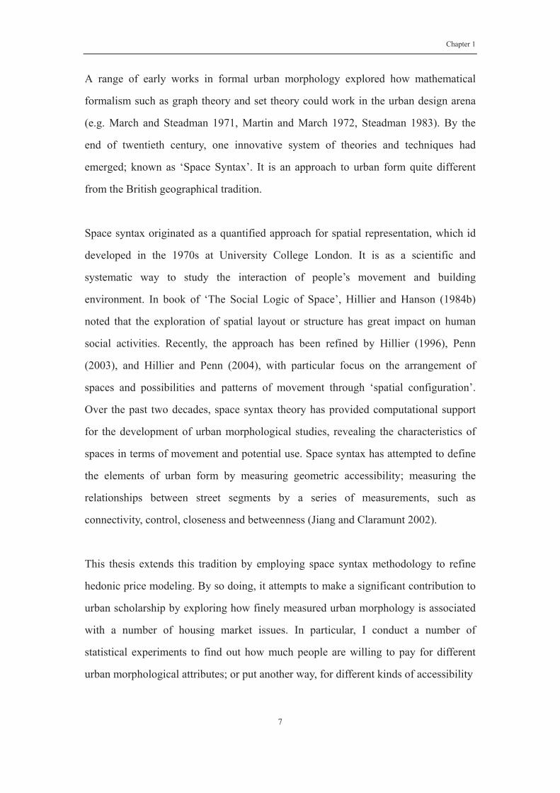
A range of early works in formal urban morphology explored how mathematical

formalism such as graph theory and set theory could work in the urban design arena

(e.g. March and Steadman 1971, Martin and March 1972, Steadman 1983). By the

end of twentieth century, one innovative system of theories and techniques had

emerged; known as ‘Space Syntax’. It is an approach to urban form quite different

from the British geographical tradition.

Space syntax originated as a quantified approach for spatial representation, which id

developed in the 1970s at University College London. It is as a scientific and

systematic way to study the interaction of people’s movement and building

environment. In book of ‘The Social Logic of Space’, Hillier and Hanson (1984b)

noted that the exploration of spatial layout or structure has great impact on human

social activities. Recently, the approach has been refined by Hillier (1996), Penn

(2003), and Hillier and Penn (2004), with particular focus on the arrangement of

spaces and possibilities and patterns of movement through ‘spatial configuration’.

Over the past two decades, space syntax theory has provided computational support

for the development of urban morphological studies, revealing the characteristics of

spaces in terms of movement and potential use. Space syntax has attempted to define

the elements of urban form by measuring geometric accessibility; measuring the

relationships between street segments by a series of measurements, such as

connectivity, control, closeness and betweenness (Jiang and Claramunt 2002).

This thesis extends this tradition by employing space syntax methodology to refine

hedonic price modeling. By so doing, it attempts to make a significant contribution to

urban scholarship by exploring how finely measured urban morphology is associated

with a number of housing market issues. In particular, I conduct a number of

statistical experiments to find out how much people are willing to pay for different

urban morphological attributes; or put another way, for different kinds of accessibility

Chapter 1

8

1.2 Research questions

This dissertation addresses three research questions relevant with urban morphology

and housing markets.

The first question has three aspects: (a) whether the accessibility information

contained in an urban configuration network model has a positive or negative impact

on housing price; (b) assuming such relationships exist, whether the network model

determinants of urban morphology are stronger or weaker than traditional locational

attributes (such as the distance to CBD); (c) whether the relationship is constant in

both disaggregated and aggregated levels.

The monocentric urban economic model and polycentric variants emphasize location,

hypothesizing that house prices decrease with a growing distance to the CBD, but

more recent studies show that distance to CBD has become less important or even

insignificant, suggesting either that people no longer choose their residential location

based on minimum travel cost to work or that work has significantly dispersed within

cities. Non-transportation factors (e.g. the distance to amenity and school quality),

have become more influential in residential locations (White 1988a; Small and Song

1992).Therefore, many scholars attempt to explore the variety of preferences for

location (e.g. the distance to a bus stop and distance to a park). However, these studies

need a priori specification within a pre-defined area, identifying local attractions

significant enough to influence locational choice systematically and measuring the

proximity of the property to these attractive places.

However, this could cause econometric bias in the estimation, such as

multicollinearity, spatial autocorrelation and omitting variables. The notion of general,

systemic accessibility has been proven to better capture location options than the

purely Euclidean distance in many studies on property value (e.g. Hoch and Waddell,

Chapter 1

9

1993), as it indicates the ability of individuals to travel more generally and to

participate in various kinds of activities at different locations (Des Rosiers et al. 2000).

However, accessibility indicators measuring attractiveness or proximity to an

opportunity are normally applied to studies at an aggregated level (e.g. Srour et al.,

2002), and disaggregated level accessibility measures still tend to rely on Euclidean

distance or time cost from a location to particular facilities.

The accessibility information contained in an urban street layout model would seem,

in principle, a suitable approach for measuring locational characteristics at a

disaggregated level without a pre-defined map of or knowledge about attractiveness

hot spots. This dissertation explores this proposition and thus contributes to this

important theoretical and methodological gap in the hedonic house-price modeling

literature.

The second question deals with the identification of housing submarkets by urban

configurational features; and comparing this approach with traditional specifications

of housing submarkets, asks whether network-based specifications produce efficient

estimation results. It is known that housing submarkets are important, and people's

demand for particular attributes vary across space. But within submarkets, the price of

housing (per unit of service) is assumed to be constant. Generally, there are two

mainstream schools of thoughts for identifying submarkets: spatial specification and

non-spatial specification. Spatial specification stresses a pre-defined geographic area

within which people’s choice preferences are assumed to be homogeneous. This is

criticized for being arbitrary. In contrast, non-spatial specification methods emphasize

accuracy of estimation, advocating a data driven approach, which is criticized for

being unstable over time (e.g. Bourassa et al.1999). These specifications for housing

submarket are widely accepted in academic and practitioner fields in most developed

countries with mature urban land markets. There is less knowledge about how to

delineate sub markets in property markets of developing countries, where the building

Chapter 1

10

type in many fast growing cities is dominantly simplex (apartments) and social

neighborhood characteristics are not long established and change quickly over time.

This is the case in most cities in China.

This question contributes to another important gap in existing knowledge, as urban

configuration features are assumed to be associated with both spatial information and

people’s preference. A network-based method could provide a new alternative

specification for housing submarket delimitation that extends the non-spatial method

by adding more emphasis on people’s choice of location indirectly. The method could

also help urban planners and government officials understand how different social

economic classes respond to the accessibility of each location.

The third question has three aspects: (a) exploring micro-dynamic effects of urban

configuration on housing price volatility; (b) asking whether this relationship is

dynamic and synchronous over both space and time and whether submarkets exist as a

result of this dynamic relationship; and (c)asking what kind street network

improvements produce positive and negative spillover effects captured in property

values.

The literature shows that most empirical analyses of house price movement focus on

exploring the macro determinants of price movements over time using aggregate data,

such as GDP, inflation indices and mortgage rates. Although some scholars state that

accessibility could be a potential geographical determinant of house price volatility at

a regional or city scale, there is little evidence confirming this relationship statistically.

One reason for that is inaccurate measurements of accessibility(Iacono and Levinson

2011). In particular, it has proven difficult to measure changes inaccessibility at the

disaggregated level, which is more reliant on Euclidean distance measures of

accessibility. The premise of the research presented in this thesis, particularly in the

chapter on China, hypothesizes that the continuous changes in urban street network

Chapter 1

11

that are associated with urban growth and the attendant changes in accessibility, are

partial determinants of micro-level house price volatility. This question is particularly

relevant in China, where the profound institutional reforms of urban housing systems

and breathtaking urban expansion, have meant numerous investments into road

network developments aimed at the urban fringe in order to facilitate the rapid

expansion of cities. The city of Nanjing, used as a case study in Chapter Six is a good

example, providing an opportunity to empirically examine the dynamic relationship

between housing price and urban configurational change.

The findings of this dissertation should be of great value to urban planners and

government officials in addressing the problem of managing urban growth efficiently,

understand the multi-scale positive and negative externalities of road networks as

captured in housing markets, assisting property value assessment for tax purposes,

and evaluating urban land use policies and planning regulations.

1.3 Thesis structures

This thesis is organized into seven chapters.

After the introduction, chapter two investigates the literature on house price

evaluation using the Hedonic price model. The approach covers several aspects,

including the fundamental theory, theoretical criticisms, issues of estimation bias, and

choice of housing attributes. In particular, the chapter focuses on the specification of

the hedonic house price function form, housing submarkets and the debates on

locational characteristics.

Chapter three provides a literature review of the methodology of space syntax-style

network analysis. The basic notion of the space syntax method and the algorithms of

two types of accessibility indices (integration and choice) areintroduced, respectively.

Chapter 1

12

Then, some key criticisms of space syntax are summarised. Finally, the chapter

reviews empirical evidence on how urban morphology interacts with socio-economic

phenomenon.

Chapters of four to six present theoretical and empirical analysis, which addresses the

thesis’ three research questions, respectively. In order to clearly delineate the

theoretical contribution of each question, separate specific literature reviews are

provided in each chapter.

Using a semi-log hedonic price functional form, chapter four adopts a part of the

metropolitan area of Cardiff, UK as a case study to examining whether urban

configurational features can impact the property value at both individual and output

area level.

Chapter five uses the same Cardiff dataset, examining whether urban configurational

features can be considered as an efficient specification alternative for identifying

housing submarkets, especially when there is no predefined spatial boundary.

Two-step clustering analysis is discussed in chapter and the results of a network

approach to housing market delineation are compared to the results of two traditional

approaches.

Chapter six setup a panel study of multi-year house prices to examine whether the

continuous changes in urban street network associated with urban growth and the

attendant changes in accessibility are partial determinants of micro-level house price

volatility. This chapter uses the case of Nanjing, China in the time period from 2005

to 2010.The Space syntax method is employed in this chapter to track changes in

accessibility within the urban street layout over time.

Finally, chapter seven presents the conclusions from the research. It also summarises

Chapter 1

13

the discussions of the three empirical chapters and presents brief reflections on the

policy implications of the results. The chapter ends with comments on the limitations

of the experiments presented in the thesis and with recommendations for future

studies in this field.

Chapter 2

14

Chapter Two:

Hedonic housing price theory review

2.1 Introduction

The most commonly applied methods of housing price evaluation can be broadly

divided into two groups: traditional and advanced methods. There are five traditional

mainstream standard recognized valuation methods in the field of property valuation:

comparative method (comparison), contractor’s method (cost method), residual

method (development method), profits method (accounts method), investment method

(capitalization/income method).Advanced methods include techniques such as

hedonic price modeling, artificial neural networks (ANN), case-based reasoning and

spatial analysis methods.

Hedonic price modeling is the most commonly applied of these. Many scholars (e.g.

Griliches, 1961) have referred to the work of Court (1939) as an early pioneer in

applying this technique. He used the term hedonic to analyze price and demand for

the individual sources of pleasure, which could be considered as attributes combined

to form heterogeneous commodities. It was an important early application of

multivariate statistical techniques to economics.

In this chapter, several aspects of hedonic modeling will be investigated in-depth,

including the theoretical basis, the theoretical criticism, estimation criticism, and its

use in pricing housing attributes, including accessibility (the subject of this thesis).

Accordingly, the conclusion will mainly focus on the theoretical aspects of hedonic

price modeling that are relevant to the question of which function form to choose in

this study.

Chapter 2

15

2.2 Hedonic model:

In regards to the theoretical foundations, the hedonic model is based on Lancaster’s

(1966) theory of consumer’s demand. He recognized a composite good whose units

are homogeneous, such that the utilities are not based on the goods themselves but

instead the individual “characteristics” of a good – its composite attributes. Thus, the

consumers make their purchasing decision based on the number of characteristics a

good as well as per unit cost of each characteristic. For example, when people choose

a car, they would consider the quantity of characteristics from a car, such as fast

acceleration, enhanced safety, attractive styling, increased prestige, and so on.

Although Lancaster was the first to discuss hedonic utility, he says nothing about

pricing models. Rosen (1974a) was the first to present a theory of hedonic pricing.

Rosen argue that an item can be valued by its characteristics, in that case, an item’s

total price can be considered as sum of price of each homogeneous attributes, and

each attribute has a unique implicit price in a equilibrium market. This implies that an

item’s price can be regressed on the characteristics to determine the way in which

each characteristic uniquely contributes to the overall composite unit price.

As Rothenberg et al. (1991) describes, the hedonic approach has two significant

advantages over alternative methods of measuring quality and defining commodities

in housing markets. First, compressing the many characteristics of housing into one

dimension allows the use of a homogenous commodity assumption; and thus, the

hedonic construction avoids the complications and intractability of multi-commodity

models. Furthermore, the hedonic approach reflects the marginal tradeoffs that both

supplier and demanders make among characteristics in the markets, so that differences

in amounts of particular components will be given the weights implicitly prevailing in

the market place.

Chapter 2

16

2.2.1 Theoretical basis

Housing constitutes a product class differentiated by characteristics such as number of

rooms and size of lot. Freeman III (1979b) argued that the housing value can be

considered a function of its characteristics, such as structure, neighborhood, and

environmental characteristics. Therefore, the price function of house can be

demonstrated as

Equation (2.1)

Where:

The , and indicate the vectors of site, neighborhood, and environmental

characteristics respectively.

Empirical estimation of Equation (2.1) involves applying one of a number of

statistical modeling techniques to explain the variation in sales price as a function of

property characteristics. Let X represent the full set of property characteristics ( ,

and ) included in the empirical model. The empirical representation of the th

housing price is:

Equation (2.2)

Where

is a vector of parameters to be estimate

is a stochastic residual term

is the implicit price respected to that characteristics

Chapter 2

17

Such as hedonic price models aim at estimating implicit price for each attributes of a

good, and a property could be considered as a bunch of attributes or services, which

are mainly divided into structural, neighborhood, accessibility attributes and etc.

Individual buyers and renters, for instance, try to maximize their expected utility,

which are subject to various constraints, like their money and time.

Freeman (1979) explains that a household maximizes its utility by simultaneously

moving along each marginal price schedule, where the marginal price of a

household’s willingness to pay for an unit of each characteristic should equal to the

marginal implicit price of that housing attribute. This clearly locates the technique

within a neo-classical economics framework – a framework that analytically

computes prices on the assumption that markets equilibrate under an ‘invisible hand’

with perfect information and no transaction costs. It is noted that although the theory

of hedonics has been developed with this limiting theoretical context discussed above,

the technique is typically applied as an econometric empirical model and does not rely

on the utility maximization underlying theory.

To understand if a household is in equilibrium, the marginal implicit price associated

with the chosen housing bundle is assumed equal to the corresponding marginal

willingness to pay for those attributes. To unpack this, I begin with considering how a

market for heterogeneous goods can be expected to function, and what type of

equilibrium we can expect to observe.

Chapter 2

18

Figure 2.1 Demand and offer curves of hedonic price function

Source: Follain and Jimenez, 1985; pp.79

Following Follain and Jimenez’s works (1985), a utility function can interpret a

household decision, , where x is a composite commodity whose price is unity,

and z is the vector of housing attributes. Assume that households want to maximize

utility subject but with the budget constraint , where y is the annual

household income. The partial derivative of the utility function with respect to a

housing attribute is the household’s marginal willingness to pay function for that

attribute. A first order solution requires , i=1,…,n, under the usual

properties of u.

An important part of the Rosen model is the bid-rent function:

Chapter 2

19

Equation (2.3)

Where is a parameter that differs from household to household.

This can be characterized as the trade-off a household is willing to make between

alternative quantities of a particular attribute at a given income and utility level, whilst

remaining indifferent to the overall composition of consumption.

Equation (2.4)

1 pictured in the upper panel of fig.(2.2) show that when solving the schedule for . 1 represented by households is everywhere indifferent along 1 and schedules

that are lower, which depend on its higher utility levels. It can be shown that

Equation (2.5)

which is the additional expenditure a consumer’s willingness to pay for another unit

of and beequally well off (i.e. the demand curve). Figure 2.2 denotes two such

equilibria: a for household 1 and B for household 2.

Chapter 2

20

Figure 2.2 The marginal implicit price of an attribute as a function of supply and demand

Source: Follain and Jimenez, 1985; pp.79

The supply side could also be considered, as p(z) is determined by the market,. When

P (Z) as given, and constant returns to scale are assumed, each firm’s costs per unit

are assumed to be convex and can be denoted as , where the denotes factor

price and production-function parameters. The firm then maximizes profits per unit

, which would yield the condition that the additional cost of

providing that th characteristics, , is equal to the revenue that can be gained, so

that .

Rosen (1974) emphasized that in fact the function is determined by a market in a

clearing condition, where the amount of commodities offered by sellers at every point

must equal to amounts demanded by consumers choosing. Both consumers and

Chapter 2

21

producer base their locational and quantity decisions on maximizing behavior and

equilibrium prices are determined so that buyers and sellers can be perfectly scheduler.

Generally, a market-clearing price are determined by the distributions of consumer

tastes as well as producer costs.

However, Rosen did not formally present a functional form for the hedonic price

function, his model clearly implies a nonlinear pricing structure.

2.2.2 Hedonic price criticism

One of the most important assumptions to come under attack is the one relating to

perfect equilibrium. For this assumption to hold, it requires perfect information and

zero transaction costs (Maddison 2001). If the equilibrium condition does not hold,

the implicit prices derived from hedonic analysis are biased, because there is no a

priori reason to suppose that the extent of disequilibrium in any area is correlated with

the levels if particular amenities contributing to the hedonic house price. The

consequence of disequilibrium is likely to be in increased variance in results rather

systematic bias (Freeman III 1993). Furthermore, Bartik (1987) and Epple (1987) also

point out that the hedonic estimation is not to the result of demand-supply interaction,

as in the hedonic model, an individual consumer decision does not affect the hedonic

price function, which implies that an individual consumer’s decision cannot affect the

suppliers.

Follain and Jimenez (1985) argue that the marginal price derived from the hedonic

function does not actually measure a particular household is willing to pay for a unit

of a certain characteristic. Rather, it is a valuation that is the result of demand and

supply interactions in the entire market. Under the restrictive condition of

homogeneous preferences – another limitation of the neo-classical model - the

hedonic equation can reveal the underlying demand parameters for the representative

Chapter 2

22

household. When all households are similar with homogenous characteristics of

income and socio-economic and supplies are different, the hedonic coefficient will be

the marginal willingness to pay. Only in extreme cases when all consumers have

identical incomes and utility functions will the marginal implicit price curve be

identical to the inverse demand function for an attribute. With identical incomes and

utility functions, these points all fall on the same marginal willingness to pay curve

(Freeman 1979). Hence, the implicit price of an attribute is not strictly equal to the

marginal willingness to pay, and hence demand for that attribute.

Another issue raised by Freeman (1979) is the speed of adjustment of the market to

changing condition of supply and demand. If adjustment is not complete, observed

marginal implicit price will not accurately measure household marginal willingness to

pay. When the demand for an attribute is increasing, marginal implicit prices will

underestimate true marginal willingness to pay. This is because marginal willingness

to pay will not be translated into market transactions that affect marginal implicit

price until the potential utility gains pass the threshold of transactions and moving

cost.

Finally, the market for housing can be viewed as a stock-flow model where the flow is

a function form, but the price at any point in time is determined only by the stock at

that point in time. This raises a concern about the accuracy of the price data itself.

Given that the data is based on assessments, appraisals, or self-reporting, it may not

correspond to actual market price. The errors in measuring the dependent variable will

tend to obscure any underlying relationship between true property value measures and

environment amenities. But the estimation of the relationship will not be biased unless

the errors themselves are correlated with other variables in the model.

Chapter 2

23

2.2.3 Estimation criticism

The hedonic price model relies on regression technology, which is criticized by some

authors for a series of econometric problems that can lead to the bias of estimation,

such as function specification, spatial heterogeneity, spatial autocorrelation, housing

quality change, multicollinearity and heteroscedasticity.

2.2.3.1 Function specification

Hedonic models are sensitive to choice of functional form, as economic theory gives

no clear guidelines on how to select the functional form. Rosen (1974a) demonstrated

that the hedonic price functional form is a reduced form equation which reflect

mechanisms of both supply and demand. A further important task facing researchers is

how to function the relationships of dependent variable and the explanatory variables

naturally, which impose an incorrect functional form on the regression equation will

lead to misspecification bias. The simple approach is the ordinary linear approach, but

if the true functional form of the hedonic equation is not linear, there will occur

inconsistent estimation in the resulting coefficients (Linneman 1980). Freeman (1979)

specified the Box-Cox transformation, which allows choice of the proper function

form based on the structure of a particular data set. Typically, hedonic price regression

models can be classified into four simple parametric functional forms;

a. Linear specification: both the dependent and explanatory variables enter the

regression with linear form.

Equation (2.6)

Where:

p denotes the property value.

is a vector of random error term

(k = 1, . . . ,K) indicates the marginal change of the unit price of the kth

Chapter 2

24

characteristic of the good.

b. Semi-log specification: in a regression function, dependent variable is log form and

explanatory variable is linear , or dependent variable is linear and explanatory

variable is log form. Equation Equation (2.7)

Where:



(k = 1, . . . ,K) indicates the rate at which the price increases at a certain level,

given the characteristics x

c. Log-log specification: in a regression function, both the dependent and explanatory

variables are their log form.

Equation Equation (2.8)

Where:



(k = 1, . . . ,K) indicates how many percent the price p increases at a certain

level, if the kth characteristic xk changes by one percent.

d. Box-Cox transform: determine the specific transformation from the data itself then

enter the regression in individual transformed form.

Equation (2.9)

Where:

Chapter 2

25

From the Box-Cox transform equation we can see if the and are equal to 1, the

model will transform to the basic linear form. If the and are equal to 0, the

model will transform to the log-linear form. If the value is equal to 0 and are

equal to 1, then the model can be the semi-log form.

2.2.3.2 Debate about the hedonic function

Unfortunately, economic theory provides little guidance, and there is no specific

function form for the hedonic price models suggested by Rosen (1974), Freeman

(1979), Halverson and Pollakowski (1981) and Cassel and Mendelsohn (1985), so it is

reasonable to try several functional forms to find the best performance. Among the

four types of function forms in hedonic literatures, the semi-logarithmic form is much

more prevalent, as it is easy to interpret its coefficients as the proportionate change in

price arising from a unit change in the value of the characteristic. Furthermore, unlike

log-log models, the semi-log model can deal with dummy variables for characteristics

that are either present or absent (0 or 1). Diewert (2003) argued that the errors from a

semi-log hedonic function are homoskedastic (have a constant variance).

Although more and more researchers prefer to use the Box-Cox transformation

function, letting the dataset drive the function form, Cassel and Mendelsohn (1985)

pointed out four inconsistencies of the Box-Cox transformation. Firstly, the large

number of coefficients estimated with Box-Cox reduce the accuracy of any single

coefficient, which could lead to poorer estimates of price. Secondly, the traditional

Box-Cox functional form is not suited to any data set containing negative numbers.

Furthermore, the Box-Cox function may be invalid for prediction, as the mean

predicted value of the untransformed dependent variable need not equal the mean of

the sample upon which is estimated. The predicted untransformed variables will be

biased, and the predicted untransformed variables may also be imaginary. Fourth, the

nonlinear transformation results in complex estimate of slopes and elasticities, which

Chapter 2

26

are often too cumbersome to use properly.

Taking least error as the choice criterion, Crooper et al. (1988) compared six function

forms: linear, semi-log, double-log, Box-Cox linear, quadratic and quadratic Box-Cox,

testing the best goodness of fit using data for Baltimore. His studies found that no

function produced the lowest i for all the attributes, although the quadratic Box-Cox

function had the lowest normalized errors. However, the linear Box-Cox function had

the lowest error variance, and based on the criterion, the linear Box-Cox performed

the best and quadratic and double-log functions the worst. On the other hand, when

variables are replaced or omitted, the Box-Cox linear function was the best of the six.

Having said all this, Halvorsen and Pollakowski (1981)rightfully pointed out that the

true hedonic function form is unknown: we can only estimate it for any particular data

set, although as I have shown, we do have methods to help choose the most

appropriate parametric hedonic function form.

2.2.3.3 Housing submarkets

Housing property cannot be regarded as a homogeneous commodity. A unitary

metropolitan housing market is unlikely ever to exist. Instead it is likely to be

composed of interrelated submarkets (Adair et al. 1996; Tu 1997; Goodman and

Thibodeau 1998; Whitehead 1999; Watkins 2001). Straszheim (1974) suggested that

the housing market is a series of single markets, which requires different hedonic

functions. According to Schnare and Stuyk (1976), housing submarkets arise when

competition in a housing market is insufficient to ensure spatial equalization of

physical housing attributes. Thus, the submarkets existence is the results of

inelasticity (or high inelasticity) of demand and supply of housing at least in a short

term. Bau and Thibodeau (1998) define housing sub-market as follows:

Chapter 2

27

“Housing submarket are typically defined as geographic area where the prices per unit of

housing quantity (defined using some index of housing characteristic) are constant.”(Bau and

Thibodeau, 1998).

Goodman and Thibodeau (1998) argue that the existence of submarket questions the

validity of the traditional assumption that urban housing markets can be modeled on

the basis of a single market-wide house price equation. Adair et al. (1996), also argue

that the failure to accommodate the existence of housing submarket will introduce

bias and error into regression-based property valuation. Orford (2000), demonstrates

that submarkets could be considered as relatively homogeneous sub-groups of the

metropolitan housing market, people’s the preference on each housing attribute may

vary in different submarkets whilst remain the same within each submarket. However,

the theory assumes that the implicit price for per unit of each housing attribute is

stationary over space, and this assumption ignores that different geographical demand

and supply characterized by different classes of people can lead to the spatial

disequilibrium of housing market in a metropolitan area. Thus, parameters estimated

by a simple hedonic function for the whole market sometimes seems misleading.

Goodman and Thibodeau (2007) emphasize that housing submarkets are important in

house price modeling for several reasons. Firstly, the assigning of properties to

housing submarkets is likely to increase the accuracy of the prediction of the

statistical models, which are used to estimate house prices. Secondly, identifying

housing submarket boundaries within metropolitan areas will increase the chance of

researchers deriving better spatial and temporal variations in their models of prices.

Thirdly, the accurate allocation of properties to submarkets will improve the abilities

of lenders and investors to price the risk related to the financing of homeownership.

Finally, the provision of submarket boundary information to housing consumers will

decrease their search costs.

Chapter 2

28

In terms of the specification of housing submarkets, Goodman and Thibodeau (1998)

stated that a metropolitan housing market might be segmented into groups of

submarkets according to the factor of demand and / or supply. Watkins (2001) also

suggests that housing submarkets exist as dwelling can generate different price due to

the interaction between segmented demand characterized by consumer groups, and

segmented supply characterized by product groups. As such, housing submarkets may

be defined by dwelling type (e.g., town house, flat and detached house); by structural

characteristics (numbers of bedroom, and building style); by neighborhood

characteristics (e.g., school quality). Alternatively, housing markets may be

segmented by age, income and race of households (Schnare and Struyk 1976; Gabriel

and Wolch 1984a; Munro 1986; Allen et al. 1995). In that case, higher income

households tend to be willing to pay more for housing (per unit of housing

services)and the attributes of other home-owners - to protect the homogeneity of

their neighborhood, life chances of children and so on. Finally, racial discrimination

may produce separate housing submarkets for majority and minority households

(King and Mieszkowski 1973). Several empirical studies of submarkets have, found

that spatial characteristics are more important than structure characteristics. Ball and

Kirwan (1977) found housing affordability and the availability of mortgage finance to

be important shapers of sub markets, despite spatial constraints. Historical

characteristics can also contribute to housing market segmentation. More recently,

scholars have been more aware of the importance of both spatial and structural factors

as the specification criterions of housing submarket (Adair et al. 1996; Maclennan and

Tu 1996).

Although, many researchers agree on a sub-market definition based on structural and

locational features, there is little consensus as to how a submarket should be identified

in practice. The most common procedure for testing submarket existence was

introduced by Schnare and Struyk (1976) and has been employed subsequently (for

example, Dale-Johnson 1982, Munro 1986). The test procedure involves three stages.

Chapter 2

29

First, hedonic house price functions are estimated for each potential market segment

in order to compare the submarket price for a `standard' dwelling. Secondly, a chow

test is computed in order to show whether there are significant differences between

the submarket specific prices. Thirdly, a weighted standard error is calculated for the

submarket model, which acts as a further `common-sense' test of the significance of

price differences for standard dwellings in different submarkets. This procedure also

enables us to do a comparison of the effects on the accuracy of the house price models

when different submarket definitions and stratification schemes are being compared.

Bourassa et al.(1999) stressed the need to test whether boundaries of submarkets are

stable over time. Adding a dynamic part to the analysis makes it even more difficult to

specify sub-market models since markets are constantly changing.

2.2.3.4 Spatial autocorrelation

A further discussion in terms of the application of hedonic price modeling is spatial

dependency, also known as spatial autocorrelation. One of the basic assumptions

underlying the regression model is that observations should be independent of one

another. However, from the first law of geography, attributed to Tobler (1970),

‘everything is related to everything else, but near things are more related than distant

things’, the independence of observations assumption is clearly a problem. Spatial

autocorrelation is concerned with the degree to which objects or activities at some

place in the earth’s surface are similar to other objects or activities located nearby

(Goodchild 1986). This is important in the sense that it is a special feature of spatial

data (Can 1990); for example, houses that are close in geographic space are likely to

have similar attributes. Generally, if the spatial effect is ignored, it is more likely that

the real variance of the data is underestimated and thus leads to bias of the results

(Ward and Gleditsch 2008). According to the works of Dunse et al. (1998), Bowen

Chapter 2

30

et al. (2001), Gillen et al. (2001), and Orford (1999), there are at least three sources of

spatial autocorrelation, including property characteristics, the evaluation process; and

mis-specification in the OLS model.

Firstly, spatial dependency exists because nearby properties, have similar property

characteristics, in particular for structural features, as the properties were developed at

the same time and also share the same locational conditions (Gillen et al. 2001;

Bourassa et al. 2005).Secondly, spatial autocorrelation also arises from the valuation

process, as the transaction price agreed between buyers and sellers will affect the

price of the surrounding area (Bowen et al. 2001), especially where valuers use the

comparison method, which is most common in the residential real estate industry.

Thirdly, mis-specification of a model can result in spatial autocorrelation (Orford

1999), when the model is missing important variables, has extra unimportant variables,

and / or an unsuitable functional form. Anselin (1988) also states that spatial

autocorrelation is associated with spatial aggregation, the presence of uncontrolled-for

non-linear relationships, and the omission of relevant variables.

Generally, spatial autocorrelation analysis is applied for testing whether the observed

value of a variable is independent of the values of the variable with neighbors. The

function of a spatial autocorrelation index is to measure the degree of interdependence

between variables, and the strength and nature of that interdependence. It may be

categorized as positive and negative, respectively. Positive autocorrelation occurs

when high or low values of the random variable tend to cluster in space, whereas

negative autocorrelation takes place when locations tend to be surrounded by

neighbors with very dissimilar characteristics. Commonly, Moran’s I test measures

spatial dependency in the residuals of a regression model, and it checks the

similarities among the housing price and attribute data in relation to the spatial

relationships (Bowen et al. 2001).If there are N observations on a variable x at

locations i, j, the formula for Moran’s I is :

Chapter 2

31

Equation (2.10)

Where:

μis the mean of the x variable,

wij are the elements of the spatial weights matrix,

S0 is the sum of the elements of the weights matrix.

The range of Moran’s I is from -1 to +1, and an expected value (zero) shows absence of

autocorrelation in samples. Moran’s I compares the relation between the deviations

from the mean across all neighbors of I, adjusted for the variation in y and the number

of neighbors for each observation. Higher value of Moran’s I indicate stronger positive

clustering, which means the values from neighboring units are similar to one another.

2.2.3.5 Housing quality change

Although the hedonic model has been used for housing market analysis for more than

30 years, and most studies rely on one-shot studies of one place at one point in time

(Richardson et al. 1990), the modeling approach has been criticized for its instability

of the coefficients over time (Case and Quigley 1991; Quigley 1995; Case et al. 2006).

According to the Dhrymes (1971) most studies consider the time variables as essential

explanatory variables, which imply that they are a proxy for change in quality over

time. Griliches (1996) constructed a hedonic price index for automobiles in an attempt

to measure the change in quality over time, and he noticed the coefficient of the

characteristics were unstable and changed over time. McMillen (2003) took an

alternative repeat sales model to identify changes in house price distance gradients in

Chicago. He employed the transaction data of Chicago from January 1, 1983 to

December 31, 1998, and he found that the distance from the CBD did not affect house

prices in the City of Chicago significantly in the early to mid 1980s. However, the

situation reversed in the 1990s as a significant CBD house price gradient was

Chapter 2

32

reestablished, and by the end of the 1990s, house values fell by more than 8% with

each additional mile of distance from the CBD. He explained that this change in

gradients was caused by a rapid appreciation of values near the city center as new

housing was built, which increased demand for housing near Chicago’s center.

Similarly, Hulten (2005) criticized the hedonic price method as failing to capture

dynamics since price inflation and quality both change over time. Inflation could lead

to an upward shift in the hedonic function because some or all characteristics become

more expensive, whereas quality change can be caused by changes in compositions of

housing attributes and by product innovation. Changes in compositions of varieties

can occur with changes in people’s income, tastes, demographics and environmental

preferences. For example, opening a new train station will affect people’s choice of

location in respect to living near job centers. On the other hand, product innovation

occurs when the cost of acquiring a number of characteristics is reduced. For example,

in the past whether the property has a fireplace can affect the property value, but

nowadays the fireplace is less significant as the construction cost for installing a

fireplace is lower.

Some scholars attempt to explore the relationship between property value and certain

attributes in temporal, such as the question of how soon the housing price will

increase due to the kind of attribute adding the value. For example, Gatzlaff and

Smith (1993) examined the impact of the development of the rail system on the

residential property values in Miami. Using hedonic model, they found that the rail

development announcement’s impact on residential property value is weak. However,

comparing a house price index for properties located near rail stations versus the

housing price index for the Miami MSA indicates a weak relative increase in house

value close to the station. Based on the results, they concluded that the Metro rail

system has little effect on accessibility improvement. Noonan (2007) examined the

effect of historic landmarks on property value in Chicago using a hybrid hedonic

Chapter 2

33

model and repeat-sales model. The results suggests that housing near landmark

buildings sold at a small premium during the 1990s.

2.2.3.5 Multicollinearity

Another issue that researchers often encounter when they attempt to estimate the

hedonic function is multicollinearity (Lake et al. 2000; Orford 2002).

Multicollinearity is a statistical phenomenon when two above exploratory variables in

a multiple regression model are highly correlated. For example, it is well known that

both traffic noise and air pollution have a negative impact on housing properties,

however, likely that traffic noise and air pollution are highly correlated, as high level

traffic flows could result in poor air quality. In this case, regression analysis finds it

difficult to tease apart the separate influence on property price, consequently the

estimation for each parameter is no longer reliable. There is no easy solution to the

problem of multicollinearity and the parameters estimated maybe implausibly large or

have the wrong sign (e.g. the opposite relationship). Sometimes, it is possible to

overcome multicollinearity by measuring the variables more accurately, or applying

principal components analysis to combine the highly correlated variables into one

index.

However, multicollinearity does not reduce the predictive power and reliability of

whole model, at least within the sample size. It only affects calculation regarding

individual predictors. There are several methods for detecting multicollinearity such

as VIF, Condition Number test and Farrar-Glauber test. The studies in this thesis use

the variance inflation factor (VIF) to measure the multicollinearity, and its formula is

as following:

Equation (2.11)

Wh

the

mul

2.2.

Het

term

sam

shou

time

cros

hete

estim

vari

cou

The

econ

of m

aggr

exam

con

con

Thu

pred

seri

Gol

ere is

other exp

lticollinearit

.3.6 Hetero

eroscedastic

m of the he

mple (Hendr

uld not be c

e series and

ss-sectional

eroscedastic

mates to b

iances are n

ld lead to un

ere are two m

nomic beha

measuremen

regation, su

mple of a b

sumers. Th

sumers, the

us, heterosce

dictor varia

es of diagn

ldfeld–Quan

s the coeffic

plicators. If

ty problem.

scedasticity

city is a ph

donic mode

ry 1995). O

correlated w

d cross secti

data (Ng

city (constan

be biased. T

no longer m

nreliable co

main source

avior of the

nt arises in

uch as censu

behavioral s

his can indu

e more the p

edastic data

able and the

ostic test, su

ndt test, Coo

cient of det

f VIF is

.

y

henomenon

el are uneq

One assump

with the dep

onal data, it

ghiep and

nt variance)

The estima

minimized, e

onfidence in

es of hetero

sample (He

n the situati

us area data

source is the

uce heterosc

possibility fo

a could bias

e outcome.

uch as Park

ok–Weisber34

ermination

more than

where the

qual (Fletch

ption of O

pendent vari

t is more co

Al 2001

) does not c

ates are con

even if the

ntervals, and

oscedasticity

endry 1995)

on where d

a, are used

e effect of d

cedasticity

or the price

s the estima

However, h

k test, Glejs

rg test and e

of a regress

n 10, it in

variance o

her et al. 20

LS is that

iables. Alth

ommonly pr

). Accord

ause ordina

nsistent but

sample size

d t and F tes

y; statistical

). A commo

data for a h

to represen

different ba

as the mor

to be lower

ations for th

heterosceda

ertest, Whit

etc. In this s

sion of expl

ndicates th

of the distu

000) or chan

the varian

ough it can

resent in stu

ding to Gu

ary least squ

t inefficien

e is increas

sts.

l methods o

on statistical

high level o

nt individual

argaining po

e the barga

r (Harding e

he relationsh

asticity can

tetest, Breu

study, the W

Cha

lanatory j o

here is ser

urbance or e

nges across

ce of the e

n happen in

udies emplo

ujarati (20

uares coeffic

nt because t

ed. Howeve

of modeling

l source of e

of geograph

l properties

ower of hou

aining powe

et al. 2003).

hip between

be detected

usch–Pagan

White test w

apter 2

n all

rious

error

s the

error

both

ying

003),

cient

their

er, it

g and

error

hical

. An

using

er of

.

n the

d by

test,

would

Chapter 2

35

be applied to detect whether there is heteroscedasticity in the error terms;

Equation (2.12)

Equation (2.13)

Step 1: using OLS procedure, obtain , and .

Step 2: Square the residual

Step 3: Regress the squared residual against a constant ,

Step 4: Compute the statistics nR2 where the n is the size of the sample and R2is the

unadjusted R-square from the step 3

Step 5: Reject the null hypothesis that if nR2>,

, the upper 5 percent point on the chi-square distribution with 5 d.f.

2.3 Housing attributes

The basic hypothesis of hedonic housing models is that housing price can be

considered as willingness to pay for a bundle of characteristics. Empirical studies

have generally grouped determining variables into three subsets:

a. Structural or internal attributes describe the physical characteristics of housing (e.g.

numbers of bedroom, swimming pool, and garage).

b. Locational attributes include the distance to major places of employment, to major

amenities (e.g. shopping mall and public facilities, etc.), and to road infrastructure

and transport access points (e.g. train station, subway station, major streets,

highways, airports, etc.).

c. Neighborhood attributes depict the quality of the economic and social

Chapter 2

36

characteristics of the neighborhood (e.g. income status and racial composition).

d. Environmental attributes describe environmental quality and environmental

amenities, such as air pollution, water pollution, noise, aesthetic views and

proximity to recreational sites or public service.

These are discussed in the following

Cha

pter

2

37

Tabl

e 2.

1 Se

lect

ed p

revi

ous s

tudi

es o

n he

doni

c pr

ice

mod

el

Type

of h

ousi

ng a

ttrib

utes

C

hara

cter

istic

A

utho

r and

yea

rs

Sam

ple

size

O

ther

var

iabl

es u

sed

Impa

ct o

n ho

usin

g pr

ice

Stru

ctur

e ch

arac

teris

tic

squa

re fo

otag

e

Sirm

ans e

t al.(

2006

)

58

the

geog

raph

ical

loca

tion

time

trend

real

med

ian

hous

ehol

d in

com

e

the

data

sour

ce

+

lot s

ize

41

+

age

71

-

bedr

oom

s 33

+

bath

room

s 50

+

gara

ge

29

+

swim

min

g po

ol

34

+

firep

lace

29

+

air c

ondi

tioni

ng

28

+

basi

c re

side

ntia

l qua

lity

Kai

n an

d Q

uigl

ey (1

970)

57

9/27

5 si

x fa

ctor

s der

ived

from

39

varia

ble

+

dwel

ling

unit

qual

ity

+

age

of st

ruct

ure

-

num

ber o

f roo

ms

+

num

ber o

f bat

hroo

ms

+

parc

el si

ze

+

Loca

tiona

l cha

ract

eris

tic

dist

ance

to o

cean

Ric

hard

son

et a

l (19

90)

9078

/109

28

19 v

aria

bles

(e.g

. num

ber o

f bat

hroo

ms,

cond

ition

,

livin

g ar

ea, a

ge, m

onth

of s

ale

and

inco

me)

-

dist

ance

to C

BD

-

dist

ance

to S

anta

Mon

ica

-

dist

ance

to S

outh

Bay

+

dist

ance

to C

BD

H

eikk

ila e

t al.

(198

9)

10 9

28

19 v

aria

bles

(e.g

. num

ber o

f bat

hroo

ms,

cond

ition

,

livin

g ar

ea, a

ge, m

onth

of s

ale

and

inco

me)

+

Cha

pter

2

38

labo

r mar

ket a

cces

sibi

lity

Osl

and

and

Thor

sen

(200

8)

2788

11

var

iabl

es (e

.g. a

ge, l

ivin

g ar

ea ,

lot-s

ize,

gar

age,

num

ber o

f

toile

ts a

nd re

build

) +

Nei

ghbo

rhoo

d ch

arac

teris

tic

Crim

e

Dub

in a

nd G

oodm

an (1

982)

58

9/11

78

50 v

aria

bles

(e.g

. crim

inal

hom

icid

e, ra

pe,p

upil

to st

aff r

atio

, and

ave

rage

teac

her e

xper

ienc

e)

-

educ

atio

n +

race

-

prim

ary

scho

ol

perf

orm

ance

G

ibbo

ns a

nd M

achi

n (2

003)

29

00/2

998/

1544

7

varia

bles

(e.g

. dew

ellin

g ty

pe, m

ean

room

s and

porti

on in

soci

al h

ousi

ng )

+

Envi

ronm

enta

l cha

ract

eris

tic

dist

ance

to h

azar

ds

Bra

sing

ton

et a

l. (2

005)

50

51

25 v

aria

ble

(e.g

. hou

se si

ze, a

ge, p

orch

, sch

ool q

ualit

y,po

rtion

of w

hite

, and

por

tion

of g

radu

cate

deg

ree)

-

dist

ance

to p

arks

Po

udya

l et a

l. (2

009)

11

,125

27

var

iabl

es (e

.g. b

rick

exte

rior,

stor

ies,

popu

latio

n de

nsity

col

lege

deg

ree,

and

par

k si

ze)

-

Oth

er c

hara

cter

istic

C

emet

ery

view

Ts

e an

d Lo

ve (2

000)

1,

550,

000

8 va

riabl

es (e

.g. a

rea,

age

, car

par

k, sh

oppi

ng c

ente

r

and

esta

te ty

pe)

-

Chapter 2

39

2.3.1 Structure characteristics

Structural attributes describe the physical structure of property goods and land parcel.

Compared with locational attributes, the structure attributes are easier to account for

and accurately perceived. Follain and Jimenez (1985) summarie the most common

structure attributes from previous research and note that measures of living space have

been reduced to lot size, floor area and the number of rooms whilst structural quality

is measured by age, style and interior and exterior quality scores.

Sirmans et al. (2005) summarizes the top twenty characteristics that have been used to

specify hedonic pricing equations. He described the total number of times a

characteristic has been used and the number of times its estimated coefficient has been

positive, negative, or not significant. Age shows up most frequently in hedonic

models and typically has the expected negative sign although it is seen to be positive

or not significant in some studies. The age effect will depend on the period studied

and the age of the city. In historic cities, age may have a positive influence on price,

but only in particular housing markets. Age in a modern part of a historic city may

have a negative influence since the quality of modern era houses is typically inferior

to those in historic quarters. Square footage is the next most used characteristics and

typically has the expected positive effect in selling price. Other characteristics that

appear frequently are garage, fireplace and lot size. Each typically has the expected

positive effect. Garage never has a negative sign but it has been insignificant in a

number of studies. Fireplace shows up negative in only a few studies and lot size

never shows up negative. Other characteristics that show up frequently are number of

bedrooms, bathrooms, swimming pool and basement. Bedrooms show up negative in

some studies but bathrooms almost never do. Research shows that a swimming pool

never has a negative impact on selling price although it has been insignificant in

certain studies, possibly because of the liability of maintenance. Basement is usually

positive but sometimes negative even insignificant in some studies, possibly related to

Chapter 2

40

endemic dampness problems in some property markets.

In addition, Morris et al. (1972), in their pilot study in San Juan, Puerto Rico,

examined structural quality by using the dimension of availability of plumbing

facilities and other service facilities such as cooking equipment, refrigeration, and

lighting. They differentiated plumbing facilities into “inside, for exclusive use,”

“inside, shared,” or “other.” These measures, which reflected the quality of the

dwelling without associating them with the locational or neighbourhood attributes,

were found to be effective proxies for measuring quality features. Kain and Quigley

(1970) investigated the impact of housing quality on housing prices. They used

measures such as condition of, exterior structure, walls, condition of floors, drives and

walks, windows, , and levels of housekeeping. These quality features (e.g., number of

bathrooms, the number of rooms and lot size) were found to have as much effect on

the price of housing.

Sirmans et al (2006) examined the effect of nine housing characteristics on housing

price that appeared in most hedonic pricing models, including square footage,

bedrooms, lot size, age, bathrooms, fireplace, swimming pool, garage, and air

condition. They found that the coefficient of the square footage, lot size, age,

bathroom, swimming pool and air condition are sensitive to some geographical

locations and the number of variables in the hedonic model but not to time, household

income, or source of data. However, garage, fireplace and bedrooms coefficients are

not affected by some geographical location, time, income or the type of data. In

contrast, Kohlhase (1991) found that the significance of structural attributes can

change over time, and may vary between nations. While attributes relating to the

number of rooms and floor area are relatively important across nations, other

attributes change with the tradition of building style or the climate.

Theoretically, a property’s structural attributes and its location within the city are

Chapter 2

41

related, since they reflect the growth of the urban structure (Muth 1969), this implies

that an element of location will be inherent within the physical structure of the

property. This is indicated in studies such as Cubbin (1970) and Kain and Quigley

(1970), which revealed a high degree of multicollinearity between structure attributes

and the results suffered from spatial autocorrelation.

2.3.2 Locational characteristics

A property represents not only a amount of structural characteristics but also set of

location specific characteristics, which has long been regarded as the fundamental

influence in the modeling of residential location. Von Thunen’s classical land use

model was the first to formally correlate value with systematic locational

characteristics – distance to a central marketplace.

The tradition of neo-classical micro-economic theory(Alonso 1964b; Muth 1969;

Mills 1972),developed Von Thunen’s model (and the underlying Ricardian value

model) to emphasisean ‘access-space’ trade-off model that describes transportation

costs as a trade off against land rents. The trade-off model was developed under the

assumption of a monocentric city on an isotropic plane with a housing market in

perfect competition. The key idea behind the monocentric model is several restrictive

assumptions such as that workplaces are spatially centralized is that accessibility to

the CBD is the major determinant of location-specific land values and site rents.

Beckmann (1973) developed models of urban housing markets based on the central

assumption that housing and employment accessibility were jointly purchased in the

residential choice decision. Most early economic studies of housing price found there

is a downward sloping housing price curve with distance from the central business

district (CBD). However, the monocentric model has inherent limitations and has

increasingly been criticized by researchers (e.g. Boarnet, 1994). The criticisms can be

summarized into three types. Firstly, many authors have noted that employment is not

Chapter 2

42

concentrated in a central business district (e.g. McDonald, 1987; Heikkila et al., 1989).

Secondly, it has been questioned whether urban commuters engage in ‘wasteful

commuting’ in their journey to work, which could also be interpreted as the question

of whether the distribution of jobs and residence is the primary determinant of the

journey to work (Hamilton and Röell 1982; Hamilton 1989). For example, if persons

do not choose their residential location to minimize their commute to work, then there

are non-transportation factors, which are also influential in residential location (White

1988b; Small and Song 1992). Thirdly, some researchers have questioned the

monocentric assumption of exogenous employment location(Steinnes 1977, 1982).

The monocentric idea that the residential location is endogenous to employment

location, but the employment location is largely exogenous to residential location is

questionable. If employment location is endogenous to residential location, the partial

equilibrium approach of most monocentric models is inappropriate.

Many scholars conclude that workplace accessibility has been over emphasized in the

urban economics empirical literature. For example, as stated by Heikkila et al. (1989):

``with multiple-worker households, multiple workplaces are common; given a high degree of

residential mobility, sites offering accessibility to many employment nodes are more valuable

because it is not very likely that successive owners will work in the same workplace''.

Richardson et al (1990) found a significantly negative value of the coefficient related

to distance from the LA CBD in 1970; and this variable was found not to influence

house prices in 1980. McMillen (2003) found that in many cities the CBD no longer

appears to exert a significant influence on house value. Take Chicago as an example,

long viewed as a monocentric city but one in which the centrality has declined

steadily in importance over time.

In fact, cities rarely have a simple monocentric structure, and the monocentric city is a

Chapter 2

43

special case of the standard urban model (Bender and Hwang 1985). Employment and

amenity centers are often located outside of the city centre, which may cause the

house price gradient to be complex (Orford 1999). Button and Taylor(2000)noted in

the 1990s, when metropolitan areas were in a state of reformulation that no longer is

the CBD the only place one may find gainful employment, as many suburban

employment center have arisen to combat its draw. On the other hand, there is little

consensus as to the appropriate method for identifying the sub-employment centre.

For example, Giuliano and Small’s clustering methods (1991), and McMillen’s

nonparametric methods (2001). Clustering methods rely on ad hoc definitions of

density and total employment cutoffs and parametric models make strong assumptions

regarding parametric form, leading to misspecification (Redfearn 2007). Empirical

research on the nature of property price with a polycentric urban context has been

scarce. For example, in the case of Baltimore, Dubin and Sung (1987) conclude that

‘the CBD appears to behave like the other secondary centre: it has an impact, but this

effect is limited to a relatively small area’. Similar results were also found by Jackson

(1979) in Milwauke and Bender and Hwang (1985) in Chicago.

2.3.2.1 Accessibility

Accessibility has been discussed in geographic contexts from numbers of perspective

(Kwan 1998). There is little consensus on the precise definition of accessibility.

Stewart described accessibility as the population–over-distance relationship or

‘population potential’, while Hansen (1959) defined accessibility as: ‘the potential of

opportunities for interaction’. Accessibility is a measurement of ‘the spatial

distribution of activities about a point, adjusted for the ability and the desire of people

or firms to overcome spatial separation’ (Hansen, 1959). Accessibility also can be

defined as ‘the ability of individuals to travel and to participate in activities at

different locations in an environment’ (Des Rosiers et al. 1999). According to Des

Rosiers et al. (2000), accessibility relates to the ability of the individual to travel and

Chapter 2

44

to participate in activities at different locations. In a transportation model,

accessibility is defined as ‘ the distribution of some defined activity measure

versus the travel impedance (time, cost and distance) to reach that activity from the

selected zones ’(Adair et al. 2000).

Ball (1973) found that while most studies showed distance variables to be significant,

not all agree on the measure of distance. Recently, more sophisticated measures of

accessibility have been proved toper form better than purely Euclidean distance in

many studies on property value (Niedercorn and Ammari 1987; Hoch and Waddell

1993). Heikkila et al. (1989) suggest considering the possibility that accessibility to

nodes other than the CBD might be important. Bowes and Ihlanfeldt (2001) proposed

that railway stations raise the value of nearby properties, as that reduce people’s

commuting costs, and station area should therefore be better able to attract retail

activity. Various researchers have explored the relationship between specific measures

of accessibility and property value, and as showed in figure (2.3), accessibility has

been measured at aggregate level and individual level. At individual level,

accessibility could account for the distance or time cost from a location to certain

facilities, such as school, transit station, employment centre, shopping centre and so

on (e.g., Landau et al., 1981, Henneberry 1998).

Chapter 2

45

Figure 2.3 Accessibility measurement types

Source: Ismail (2005)

Debrezion et al. (2006)explored the impact of the railway network on house price in

the Netherlands by hedonic price approach. The railway access variables the authors

used include the distance to railway station, the frequency of train services and to

distance to railway tracks. They found that housing in close proximity to a railway

station commands a market price that is about 25% more expensive than equivalent

housing at a distance of 15km or more from a station. Munoz-Raskin (2010)paid

attention on the relationship of bus rapid transit and property values within walking

area. He found housing market places value premiums on properties in immediate

walking proximity of BRT feeder lines.

In contrast, Andersson et al. (2010) examined the effect of High-speed rail station (a

long-distance rail) accessibility on real estate price in Taiwan. The estimated results

show that HSR accessibility has at most minor effects on house price. Rolon (2005)

also found a new station does not bring substantial accessibility improvement and the

marginal effect on land and property values is negligible. However, there was a

negative impact of proximity to a transit station due to the noise, vibration, pollution,

visual impacts and safety issues (Bowes and Ihlanfeldt 2001).

Accessibility

Aggregate (Zonal index) Individual (distance / time involved to move from a house to centain facilities)

Employment centre

Public servieces such as schools

Shopping centre

Public transportation

General practitioners

Chapter 2

46

However, at the aggregate level, accessibility can be considered as a point of

attractiveness or proximity to an opportunity. For example, Hwang and Thill (2010)

examined the impact of job accessibility on housing price in the Buffalo and Seattle

metropolitan areas. They compute a travel-time based job-accessibility measure at the

employment level of census tracts, according to Hansen (1959)’s formulation. The

results suggest that suburbanites are more willing to pay for additional increase in job

accessibility in housing consumption than urban residents in the Buffalo-Niagara Falls

MSA, whereas the situation is opposite in Seattle.

Song and Sohn (2007) also criticized accessibility measures based on distance from a

housing unit to the CBD, regional and commercial center, arguing that it cannot

capture the overall level of accessibility for retail service. They applied a spatial

accessibility index to evaluate the effect of enhanced access to retailing in the single

family housing market in the city of Hillsboro, Oregon. This spatial accessibility

index considered the numbers of neighborhood retail store, the size of retail store, as

well as the distance to the retail store by units of census block (e.g. Weibull, 1976,

Shen 1998). The results showed that spatial accessibility to retailing as a service is

capitalized into residential price.

Adair et al. (2000) focused on the relationship between accessibility and housing price

in the Belfast urban area. Instead of traditional studies using the CBD as a reference

for accessibility indicator, they calculated the accessibility index by considering all

trip attractors and generators in the area of 182 traffic zones with sample size of2648.

For whole housing market, they found accessibility is of little significance in

explaining variation of house prices. However, the authors found that accessibility can

be an important influence at sub-market level, particular in low-income areas.

Johnson and Ragas (1987) found that the biggest obstacle to finding declining rent

gradients within a small area is that there are many other confounding factor that

Chapter 2

47

affect the land rent other than just spatial locational characteristics.

Another issue emphasized by Song and Sohn (2007) is the inaccuracy of the

accessibility measure due to spatial aggregation. Some spatial information is lost and

become insignificant as ‘households in each zone or area are typically represented by

a single point (i.e. centroid or weighted center) in calculating distance to and from the

zone’. Furthermore, they argued that the arbitrariness of spatial units could distort the

real accessibility level of individual household. Cheshire and Sheppard (1997) also

argued that much of the data used in hedonic analyses still lacks land and location

information. Different accessibility indices can interpret the different locational

information but not all the indices have proved to affect housing value. Besides that,

these aggregate empirical studies generally have not found accessibility to be as major

a factor in controlling residential mobility as traditional trade-off models imply (Adair

et al. 2000).

2.3.3 Neighborhood

Neighborhood attributes are also typically included in the estimation of housing price

models. Important among these are income level (which is a surrogate for among

other things, neighbor externalities, the ‘snob’ factor, quality of housing, level of

expenditure on housing investment and maintenance, school quality and so on).

Generally, higher income neighborhoods are assumed to be of higher quality (e.g.

higher quality education and lower crime rate). This leads to the idea that all

households prefer to live in higher income neighborhoods. Set against this is the

observation and theoretically plausible idea that households prefer to live in

neighborhoods dominated by households similar to themselves (Gans 1963). Hedonic

models of housing values that use a set of social and economic status variables (in

terms of age, income, ethnicity and lifestyle), controlling for neighborhood and

amenity quality (e.g. school) can help tease out these effects.

Chapter 2

48

2.3.3.1 School quality

There is a widely recognition that school quality is the most essential determinant of

housing price, in particular within the US. and UK contexts, as it is close related with

local property tax bands. Generally, in the field of education, some author choose a

indicator to control for school quality, such as pupil-teacher ratio and standardized test

scores (e.g. Oates, 1969, Haurin and Brasington, 1996).

Dubin and Goodman (1982) estimated the impact of school characteristics and crime

measure on 1765 house prices in Baltimore in 1978. They measures of school

characteristics by the pupil-to-staff ratio, average teacher experience, the percent of

staff with masters degrees or above, and a battery of third and fifth grade test scores.

As the school variables were highly correlated, they use principle component analysis

to reduce the data. They confirmed the school characteristics had a significant effect

on house price, but it is still difficult to determine which school characteristics

contribute more effect.

Hefner (1998) examine the impact of school characteristics on house price by

conducting two measurements for school quality. The first measurement focus on

management, including teacher’s salary, teacher / pupil ratios, teacher tenure, and

percentage of teachers with advanced education degrees. The second measurement is

considered by support for and participation in gifted and talented programs. He found

that administrative and leadership choices made by school and parents can increase

the prices of surrounding properties.

Gibbons and Machin (2003) investigated the impact of primary school performance

on housing prices in England with a pooling data set of 7444 “postcode area” in the

years 1996-1999. They serve school type as the instrument for school quality, and

Chapter 2

49

find a positive effect of local school quality on house prices. The results show that one

percentage increase in the proportion of children meeting raises property values by

0.67%.

However, the question of how change in school characteristics relate to changes in

real estate value remains open in part because, as Mieszkowski and Zodrow(1989)

note, many existing efforts to determine the extent of capitalization have been flawed

due to inadequate data.

2.3.3.2 Social economics status and ethnicity

The socio-economic characteristics of the neighborhood, such as the social status and

population characteristics (in terms of age, income, ethnicity and lifestyle) of a

neighborhood, also play a role in the choice behavior of house buyer, and therefore

have an effect on house price (Visser et al. 2008). Dubin and Sung (1990) showed that

the social-economic status and racial composition of the neighborhood affect housing

price more than the quality of public services. Racial segregation behavior studies in

some US cities (Harris 1999)may influence housing price, depending on a

community’s willingness to pay to keep its identity

Baumont and Legros(2009) examined the impact of neighborhood on the housing

value in the Metropolitan Area of Paris. Social capital, social status, social

externalities and urban renewal policies have positive or negative impacts on housing

prices.

Schafer (1979) looks at Boston 1970 census data. When the data are divided into

submarkets defined as the central city ghetto, the central city transition area, the

central city white area, and suburban white area, he reports that price differentials paid

by blacks vary greatly, depending on the submarket. He find that house prices are

Chapter 2

50

higher in the ghetto and transition area, relative to the white area.

Dougherty et al. (2009) measure the effect of both elementary school test scores and

racial composition on household’ purchase choice over a 10-year period. Overall,

while both test scores and race help explaining the variation in housing price

significantly, and they found that the influence of school performance declined, but

racial composition became nearly seven times more influential during the study

period.

Differences in house prices across racial groups have been carefully analyzed in the

past. As Yinger (1979) and Chambers (1992)point out, it is crucial to include

indicators for the household, the neighborhood, and the submarket, while controlling

for the characteristics of the house when testing for price differentials. If relevant

characteristics are excluded, the estimated coefficients will be biased.

2.3.4 Environmental

Since Ridker and Henning’s (1967) pioneering study, there has been growing interest

in using property value as a source of information on the benefits to be expected from

controlling environment disamenities. Or more generally, property price models have

become one of the common ways of valuing environmental externalities. Most

commonly the method is applied to variations in housing prices which reflect the

value of local environmental indicators, and variety of empirical studies have used a

single environment indicator in a hedonic price model(Anderson and Crocker 1971;

Wilman 1981; Murdoch and Thayer 1988). Generally, environmental characteristics

can be subdivided into two categories environmental quality and environmental

amenities. Environmental quality includes air pollution, water pollution, or noise,

while environmental amenities can be interpreted as aesthetic views and proximity to

recreational sites.

Chapter 2

51

2.3.4.1 Environmental quality

Some studies have examined the impact of environmental quality of air,, water, or

traffic on house price using hedonic models. Generally, these studies show that urban

disamenities have a negative effect on house price, which means people have a low

demand and do not have the willingness to pay for more on these characteristics – on

the contrary, they are willing to pay more for less of them. Day et al. (2007) and

Bateman et al. (2001) consider aircraft noise, while Schipper et al. (1998) and Nelson

(1982) assess the impact of multiple resources of noise from transport. Air quality has

been evidenced to have a negative relationship with property value (Graves et al. 1988;

Smith and Huang 1995). Water quality, such as pH level, clarity or visibility has been

found to be positively and significantly related to sale price (Steinnes 1992; Michael

et al. 1996). Proximity to hazardous waste sites unsurprisingly have a negative impact

on property value (Kiel 1995; Farber 1998).

Brasington et al. (2005) use the pollution site data of Ohio in US to examine the

relationship between house price and environmental disamenties. They used spatial

autoregressive method to confirm that nearby point-source pollutants depress house

price. Epp and Al-Ani (1979) studied waterfront residential properties located along

small rivers and streams in Pennsylvania and found that pH levels low enough to limit

recreational use affect housing price. They found that acidity from minerals and

carbon dioxide, which affects pH levels, significantly influenced housing price.

A distinction can be made between studies principally aimed at deconstructing house

price and those undertaken to value an environmental ‘bad’. It is likely that the latter

kind of impact studies may not be so comprehensive in identifying a full range of

independently predictive variables. Such evaluations have been criticized for

difficulties in capturing imperfect knowledge on the attributes of each location and

Chapter 2

52

measuring intangible influences and individuals’ perceptions (Wardman and Bristow

2004).

2.3.4.2 Environmental amenities

As mentioned above, proximity to a certain environmental amenity, such as a river,

and open space, could be considered as a dimension of accessibility adding value to

property values. Stegman (1969), Richardson (1977) and Pollakowski (1982) show

that house prices are also determined by the environmental attributes of the location,

which connote lower accessibility of areas peripheral to the city centre tends to

outweigh increased access to open space. Gillard (1981) argues: “even when a park

may not be used for recreation because of crime problems, it may still be valued for

aesthetic reasons by residents with a view of the park”. McLeod (1984) discovered

that the river views were particularly important, and had a greater influence than a

view of park. In particular, industrial, business and transportation land uses can have a

negative effect upon property with respect to aesthetic qualities (Powe et al. 1995).

Public open space and urban parks could enhance the economy in environment, as

well as quality of life, by improving air quality, providing recreational opportunities,

and enhancing aesthetic value, among many other benefits (Nowak and McPherson

1993). Previous research have revealed that the price of house increases with

proximity to nearby parks (Tyrväinen 1997; Thorsnes 2002), while, other studies

reveal that increasing the size of urban parks increase the housing values nearby

(Tyrväinen 1997). This lends weight to the idea that it is size of parks rather than

number per se, that matter in meeting the open space needs of a city.

Poudyal et al. (2009)examine how the demand for green parks captured by property

value. They employed a traditional hedonic price model to confirm that urban

recreation parks increase nearby property values. Increasing the average size of parks

Chapter 2

53

by 20% from the current level increased the per household consumer surplus by 160

dollars.

Netusil (2005), investigated how far open space can affect house price, taking the

empirical study of Portland, Oregon. At the radii of 30 meters to the open space, the

study found that impact of locational advantage on n the sale price of homes is

insignificant. However, at distances greater than 30 meters and up to 450 meters from

open space, homes were found to sell for statistically greater price than homes located

over 450 meters from open space.

Lutzenhiser and Netusil (2001) used the same data, to explore the open space effect

more deeply. They classified open space into urban park, natural park and specialty

park, and found of great significance were natural area parks-homes within 450

meters. Other types of open space having a statistically significant influence include

golf courses (13.3%), specialty parks/ facilities (8.5%) and urban parks (1.8%). They

find being proximity to open space does have positive impact on property values, but

this is still dependent on the type of open space and distance from the open space.

Anderson and West (2006) explored the effect of neighborhood parks, regional, state,

federal parks,natural areas and cemeteries on property value in the Minneapolis-St.

Paul metropolitan area. They find that the value of properties proximity to

neighborhood parks and special parks falls respect to the distance to the CBD

increases where has high population density and income. The benefits of proximity to

neighborhood parks on housing price become higher when neighborhood has more

children.

2.3.5 Others

In addition, there are some local context attributes, which influence property values,

Chapter 2

54

for example, Tse and Love (2000) found that a cemetery view has a negative impact

on a property’s price in Hong Kong. Generally, dwellings that have a cemetery view

are not accepted, as that is bad fengshui (geomancy).

Interestingly, there have been some studies that demonstrated the influence of

fengshui beliefs in the power of “lucky” and “unlucky” properties. For example,

Bourassa and Peng (1999b), who used sales transactions for 1989 to 1996, found that

lucky house numbers (e.g. 3, 6, 8, and 9) have significant positive hedonic prices and

are capitalized into the sale prices of houses in Auckland, New Zealand. Chau et

al.(2001) also found similar results in the predominantly Cantonese society of Hong

Kong. Their results, however, showed that lucky floor numbers (e.g. 8, 18, or 28) are

sold at significantly higher premiums during periods of property boom than during

property slumps.

2.4 Summary

This chapter presents a wide-ranging literature review of hedonic price models, which

can be summarized from a numbers of aspects.

Firstly, based on Rosen’s work (1974), it is possible to state that under a perfectly

competitive market, and when demand equals supply, the implicit price of each

attribute in the hedonic price model is the price people are willing to pay for each

characteristic. However, there are many scholars who have criticized Rosen’s hedonic

price estimation for the assumption of market equilibrium, in which case the implicit

price of an attribute estimated is not strictly equal to the marginal willingness to pay.

Secondly, it has been noted that economic theory gives no clear guidelines on how to

select hedonic price functional form. Since, the study area of the first two empirical

studies of this thesis is a part of metropolitan area of Cardiff, UK, and Orford (1999)

Chapter 2

55

explored the impact of locational externalities on housing price in Cardiff, choosing

the semi-log function form, this study will follow Orford (1999)’s approach. This is

further backed up by the consensus in the literature that semi-log equations have a

more meaningful and intuitive interpretation.

In addition, the literature reviewed also indicates that the hedonic price model suffers

from a series of potential econometric issues, which could lead to estimation bias,

such as spatial autocorrelation, multicollinearity, heteroscedasticity, and

non-measurement of housing quality change. Thus, several types of econometrics

tests will be applied in the chapters that follow, to make sure the models correctly or

as accurately as possible, estimate the implicit prices of housing attributes, including

accessibility. Among all these econometric problems, multicollinearity is most fatal

for the estimation, as it can result in an coefficients with opposite signs to their real

relationship. Therefore, it is necessary to specify the function form, and choose the

variables carefully.

Thirdly, despite of the importance of housing submarkets, there is little consensus on

how to specify submarkets, or identify their boundaries. Thus, this study attempts to

contribute to the theory and practice of identifying housing submarket using hedonic

price models. The traditional method mainly emphasizes that within geographic area

the price per unit of housing characteristics is constant, which means within a certain

space, people have identical choice preferences. In that case, they could use school

districts, postcode areas, and so on, and even include building types to specify the

housing submarket. However, there arises a question of how to specify housing

submarkets where the building type is homogeneous, and the price per unit of housing

characteristics is not constant within some geographic unit. Indeed, some scholars

have approached this matter using cluster analysis for non-spatial information by

minimizing estimated error for social economics indices, These alternative methods

are criticized since the results are unstable over time, they require high quality

Chapter 2

56

database and are difficult for policy-analysts to interpret. The innovative method I

explore in this thesis is to see if detailed morphological metrics can be used in

defining housing sub-markets. This takes the discussion of accessibility in hedonics a

step further, to see if fine-grained systemic accessibility measures, taken from an

urban grid, can not only help refine the prediction of individual house prices but also

help define geographical areas with stable and homogeneous valuations of housing

attributes.

Fourthly, it is found that housing attributes can be divided into structural attributes,

locational attributes, neighborhood attributes and environment attributes. Based on the

discussions above, it is found that there is a debate regarding the locational attributes

that influence house price: empirical evidence can be contradictory. The New Urban

Economics theory suggests that in a monocentric model, emphasis on the location (the

distance to CBD) is most essential for property value, because it accounts for the

minimum travel cost, time and distance behavior. The result is a negative gradient

curve demonstrating the relationships between distance to a centre and housing price

in markets. However, due to urban expansion and polycentricity and the growing

complexity of urban systems, many empirical studies have found that the power of

location attributes have become weak. Current studies measure accessibility at both an

aggregated and disaggregated level. However, aggregated measurements apply

advanced algorithms calculating potential opportunities or attractiveness, which have

been criticized for the loss of spatial information when aggregated. By contrast,

disaggregated measurement requires a prior specification for terminals (such as bus

station, train station), and they mainly rely on Euclidean distance measurement.

Hence, the focus of this thesis attempts to contribute the hedonic price theory by

following aspects:

Firstly, previous studies need a priori specification within a pre-defined area,

Chapter 2

57

identifying the impact of local attractions on housing property, and most of them

ignore the spatial information contains in street layout, which is most essential

element in the field of urban planning. Furthermore, compared with tranditional

measurement for locational attributes, the accessibility derived from urban

configuration does not require a priori knowledge and can be easily employed at

disaggregated level.

Secondly, despite previous specifications for housing submarket in developed

countries, there is less knowledge about how to delineate sub markets in property

markets where the building type is simplex (apartments) and social neighbourhood

characteristics are not long established and changing quickly over time, such as most

cities in China. Thus, I attempt to establish a new framework for delineating

submarket in that situation, by clustering urban configuration features, as urban

configuration features are assumed to be associated with both spatial information and

people’s preference.

Thirdly, there has been little evidence of the micro-level determinants of house price

volatility in urban land use planning. It is known that China is undergoing a process of

rapid urbanization, which in terms of scale is perhaps the largest the world has ever

experienced. Although some researchers have investigated the impact of accessibility

value, they have failed to confirm the dynamic relationship. Thus, I posit that

transformations in urban configuration accompany the urbanization process; and that

the corresponding continuous changes in street network configuration associated with

urban growth and the attendant changes in accessibility are one of the key

determinants of micro-level house price volatility in a city.

Chapter 3

58

Chapter Three:

Space syntax methodology review

3.1 Introduction

Space syntax is a street network method, which was developed in the 1970s at the

University of London as a way to quantify urban morphology features and record

movement and interaction within cities and buildings. In the book of The Social Logic

of Space (Hillier and Hanson 1984), they firstly argued that spatial layout or structure

has a great impact on human social activities. Recently, the approach was refined by

Hillier (1996), particularly focus on the arrangement of spaces and possibilities and

patterns of movement through the ‘spatial configuration’. Over the past two decades,

space syntax theory has provided computational support for the development of urban

morphological studies, revealing of the characteristics of spaces in terms of movement

and potential use. Indeed, space syntax attempt to define the elements of urban form

by geometric accessibility, measuring the relationships between street segments by a

series of measurements, such as connectivity, control, closeness and betweeness

(Jiang and Claramunt 2002).

Indeed, as a technique, space syntax is powerful and successful, as it can describe a

complex urban configuration system, providing direct interpretation to help architects,

urban planners and sociologist to understand the impact of spatial configuration on

social activities both theoretical and practical. For example, for the regeneration

project at Trafalgar square, London, the Space Syntax research method provided an

initial insight of tourists’ activity patterns in the Trafalgar Square.

Despite its success, there have been critics of the space syntax research method,

Chapter 3

59

mainly focusing on definition of axial lines and the unique set of axial lines. For

example, Ratti (2004) criticized that the appropriateness of ‘axial maps’ for describing

the urban spatial structure. It has also been suggested that the definition and

theoretical meaning of the axial map is not well-enough linked to other

graph-theoretic representation of street network (Steadman 2004).

The motivation of this chapter is to provide deeper insight into the space syntax

method, discussing several issues. Firstly, what is different about space syntax

network analysis compared with traditional geographic network analysis assessing

accessibility? Secondly, the algorithm of the space syntax method and three type of

accessibility measurement of space syntax are discussed. Thirdly, some key criticism

of space syntax will be summarised. Fourthly the social economic fields that the space

syntax method has been applied to will be discussed.

3.2 Overview of urban morphology analysis

The study of urban morphology, frequently referred to urban form, urban landscape

and townscape, has an extensive literature in three genres. Firstly, in field of human

geography, especially in Britain, there is an “indigenous British geographical

tradition”, which heavily influenced by M.R.G. Conzen. Conzen develops two of his

key ideas, the burgage cycle, and fringe belts. The Conzenianis more interesting in the

description, classification and exemplified the characteristics of present townscapes

based on the survey. Recently, the typical works contributed to of this tradition are

from Whitehand (1967; 1972, 1987a, b; 1992)and Slater (1988)..Additionally, by

contrast, European traditions (e.g. Caniggian School) takes the views from architect,

emphasizing the components of the urban structure, including its elements, structures

of elements, organism of structures(Sima and Zhang 2009). In architecture and

planning theory. Many scholars concerned urban morphology with prescriptive and

utopian for ideal cities’. For example, The Garden Cities of Howard (1965), Le

Chapter 3

60

Corbusier’s Ville Radieuse (Corbusier and Guiton 1981),and Wright’s Broadacre

(Wright 1935)are the outstanding examples of this genre.

However, the most prominent exponents of the critique from Lynch (1960), Jacobs

(1961) and Alexander (1964, 1974), requires to think city planning from anthropology

perspectives, which should be based on observation of what actually works in real

cities. This sowed the seeds of a mathematical approache for quantifying urban

morphology.

Alexander’s work first attempt to introduce formal mathematical concepts into the

debate. Some scholars interested in bringing mathematical tools into the realm of

urban morphology, in particular graph theory and set theory, and attempted to link this

idea with what works in the urban design arena (see. March and Steadman 1971 ,

Martin and March 1972 ,Steadman 1983 ). For example. Q-analysis (Atkin 1978) was

also influential. Work focusing on possible graph representations of urban form

(Krüger 1979) exemplifies the approach. Under this background, the method of space

syntax was gestated by Hillier and Hanson (1984b), which is based on a graph

representation describing cities as systems of open space.

3.3 Accessibility types

“Accessibility is a concept that has become central to physical planning during the

last fifty years.” (Batty 2009).

In the field of population geography, Stewart (1947) firstly used the concept of graph

theory defining the gravitational potential by the weighted sum of forces. Hansen

(1959) and Wilson (1970) started with a graph theory view to explore the spatial

system, identifying accessibility as a key element in spatial interaction, while Haggett

and Chorley (1969) established the central analysis approach to analyse spatial

Chapter 3

61

relationships.

Batty (2009) summarized three types of accessibility. Firstly, type one accessibility

defines how proximate or `near' an individual is to `opportunities', measuring the size

of the opportunity at some other place or location and inversely moderating the cost of

accessing the opportunities by the distance or time. The other two types of

accessibility are based on a network. Type two accessibility more focus on the

Euclidean distance between one location and another, measuring this as the sum of the

shortest routes in a planar graph.This measurement is popular in traffic models, and

high accessibility normally is associated with minimum distance, travel time and

travel cost. In the metric geographical network analysis, nodes or vertices are defined

as the intersection or junction of streets, while the links or edges are street segments

linking two intersections. This is called the prime approach. In the last twenty years, a

third type of accessibility measurement has emerged which seems more abstract. The

type three accessibility is based on the dual approach, which defined on the links of

the original graph, rather than the nodes, applying degree( ) (control), closeness ( )

(“integration”in space syntax), and betweenness ( ) (“Choice” in space syntax) as

measurement of centralities (Bavelas 1948, 1950; Leavitt 1951; Shimbel 1953; Shaw

1954, 1964).

The accessibility measured by Space syntax method(Hillier and Hanson 1984b)is

belongs to the third type, which is also called dual approach. It is more abstract,

focusing on links (street) connection in a planar graph. Similar dual approach methods

have also explored gradual directional change (Dalton et al. 2003), characteristic point

(Jiang and Claramunt 2002), street-name change (Jiang and Claramunt 2004).

Chapter 3

62

Figure 3.1Conventional graph-theoretic representation of the street network

Source: (Batty 2004a)

Many researchers have discussed the substantial differences between the prime and

dual approach, showed in figure (3.1), and arguing which approach is more effective.

Batty (2004a) states the dual approach breaks the clear links between the Euclidean

and topological space and also making the visual analysis more difficult, compared to

the prime approach, he agrees that both methods are powerful to explain the same

problem. Porta et al.(2006) introduces a new geographical network analysis

methodology, known as multiple centrality assessment, based on the prime approach.

Comparing results for the two methods, they point out that the prime approach is not

efficient in measuring the closeness and is much more fragmented than the dual

method, which is more generalized. However, he emphasizes that the prime approach

is more compatible with other fields, and is more subjective, intuitive and practical.

Hillier and Penn (2004) emphasises that the dual approach use of topological distance

prevents border effects.

3.4 Space syntax algorithm

What is original to space syntax is the important insight that the pattern of movement

Chapter 3

63

in a city or urban area is likely to be shaped to an extent by the topology of its route

network alone. The basic analytical procedure of the original space syntax method is

divided into two steps. The first step is to create an axial map, of a certain area at any

given scale. At the early stage, the axial map is based on experiences, which starts

with identifying the fattest convex spaces. A 'Convex space' showed in figure (3.2),

can be defined as polygons where no lines can be drawn between any two points (x, y)

in the space which go outside the area. The longest line indicate the most optimal

convex space with the maximum perimeter ratio. After identifying the fattest convex

space, it is possible to draw the longest axial lines within the convex space and then

draw the second longest axial and continue until all the convex spaces are covered.

The whole process should result in the fewest axial lines representing a

one-dimensional system of the spatial layout (Hillier and Hanson 1984b). Space

syntax makes a default assumption that people will move where they can see, and

'Convex space' could indicate people’s movement in a visual area. Urban space

could be decomposed into numbers of the 'Convex space' by people’s visual zone

contained in urban spatial structure or morphology , thus, the urban space could be

transformed into line-line graph with `longest and fewest' axial lines.

Chapter 3

64

Source: (Hillier and Hanson 1984b)

The results in the complex urban configuration system being represented as a one

dimension graph G (N, K), a mathematical entity defined by two sets, N and K. The

first set, N, denotes a nonempty set of N elements called nodes, vertices, or points,

and K is a set of K elements containing unordered pairs of different nodes called links

or edges. Once the representation of morphology has been created, measures of spatial

characteristics can be analyzed. Each axial line represents a node N in the graph and

each intersection between lines represents a link K. An indicator for measuring

non-metric topology is depth, which is defined by the number of turns from one axial

line to another line, or the links from one node to another node. Depth can be used to

measure patterns of line connectivity called integration(Steadman 1983; Hillier and

Hanson 1984b). This line graph approach has proven to be unexpectedly successful in

predicting urban movement and measuring urban structure change(Hillier et al. 1993a;

Hillier 1996).

1 2

5

4 3

Figu

Sour

Figu

base

(198

follo

1.

ure 3.3 calcula

rce: author

ure (3.3) sh

ed by accou

84),The for

ows:

ation of depth

ows how sp

unting the n

rmula for in

value of each

pace syntax

numbers of

ntegration o

65

h street

integration

f depth. Acc

of space sy

n value is ca

cording to H

yntax axial

alculated for

Hillier and

lines, has s

Cha

r each axial

Hanson’s w

several step

Equation (

apter 3

l line

work

ps as

3.1)

Chapter 3

66

Where:

K is the total number of nodes (axial line) in a graph

is the numbers of depth from node to node .

2. Mean depth (MD) = Sum Depth (SD)/ (K - 1). Equation (3.2)

3.Relative Asymmetry (RA) = 2 (MD - 1)/ (K - 2) Equation (3.3)

4.Real Relative Asymmetry (RRA) = RA/ Dk Equation (3.4)

Where:

denotes the total depth of the root in a diamond-shaped

graph

5. Integration = 1/RRA Equation (3.5)

Relations of depth are derived from the notion of asymmetry, as spaces can only be

deeper than other spaces when passing through intervening spaces to arrive to them.

Mean Depth provides the basis for RA, which provides a normalization of the mean

depth measure between the deepest a node could possibly be (at the end of a sequence)

and the shallowest it could be (when all other nodes are directly connected to it). This

will give a value between 0 and 1, with low values indicating a space that tends to

integrate the system, and high values a space, which tends to be segregated from the

system.

RRA provides a relativisation to allow for comparisons of depth between different

sized spatial system. RRA eliminates the effect caused when real spatial systems get

larger (are composed of more nodes). With a larger system (area) a node becomes

relatively shallower when considered relative to how deep they could possibly be

Chapter 3

67

given that number of nodes. Normally, it allows us to compare the integration value

for different urban system, such as London and Beijing; which requires eliminating

the effects of the size on the RA of any space.

Source: www.spacesyntax.com

Researches using the space syntax methodology, utilize the so called global

integration (RN) method to measure the relative accessibility of a space within a

spatial system, measuring how many locations in the city are relatively strongly

integrated (connected) and how many are less integrated and probably belonging to

the city fringe. Higher integration values are assumed to correlate with higher rates of

movement and activity. Spaces with few connections that lie “deep” within a system

have lower integration values and often experience lower levels of activity. In the

space syntax graphic, red lines represent the highest integration value; dark blue lines

represent the lowest integration value, in other words, areas with the highest level of

Chapter 3

68

segregation. Integration proves to an important spatial variable that correlates well to

social activities such as movement and interaction (Hillier 1996; Penn et al. 1998).

Local integration (R3) measures accessibility up to three steps away and in terms of

axial line, means a topological distance of three turns. There is evidence that suggest

that integration at a local level correlates strongly with local pedestrian movement,

meaning short trips to local destinations. It has also been shown to correlate with the

movement of “locals” or “inhabitants”, as compared to non residents and visitors who

enter the spatial system from the outside (Hillier and Hanson 1984; Hillier 1996).

There are other notions in the space syntax method theory, for example, the notion of

‘Connectivity’, which measures the degree of intersection or one step possibilities of

each axial line (Hillier 1996). The notion of ‘intelligibility’ is defined as the degree to

what can be seen and experienced locally in the system (Hillier 1996). The

‘intelligibility’ value is calculated by the degree of linear correlation between

connectivity and global integration value (Hillier and Hanson 1984). ‘Synergy’,

denotes the degree of linear correlation between R3 and Rn, which is used to mitigate

the influence of system size (Hillier et al. 1993a).

This broadly describes the original formulation of space syntax. There have been

significant developments beyond this, which I will consider later in this chapter. First

though, I summarize some of the basic method’s criticism.

3.5 Critics of the space syntax method

Space syntax methodology has been developed for more than 20 years since its first

publication in 1984, and is widely adopted for the analysis of urban configuration

structure and social economic prediction. However, controversies here also come with

its success. The debates mainly focus on three aspects as follows:

Chapter 3

69

Firstly, its prediction ability is weak. Space syntax in its original topological

formulation is criticized for only considering topology distance and ignoring other

distance metric or 3D information about the urban system or building system, such as

building height, land use, transportation infrastructure. For example, in terms of early

building pattern analysis, Architect Lawrence (1990) and sociologist Edmund Leach

(1978) pointed out that in a cultural context the syntactic arguments were insufficient

to infer the social dynamics only with a building's floor plan. Similar sentiments were

expressed by Osman and Mamoun (1996), who state that the boundaries between

spaces are normally set by some kind of furniture rather than by physical barriers, and

note that space syntax only models open floor plans.

Recently, Ratti (2004) criticized space syntax systematically, “How is it possible to

tell so many things about the urban environment with such a limited amount of

information that is, after having dismissed data such as the height of buildings and

the size of streets”. He also argued that topological distance is unacceptable, as the

topological distance facing“ New Yorker living on Fifth Avenue between 111th and

112th Streets going to Central Park North round the corner (two changes of direction)

is the same for him going to Columbus Circle ” (Ratti 2004). In fact, the

Columbus Circle is much further away.

Steadman (2004) points out that the space syntax method seems to be problematic at

the large urban scale. Movement along a straight but congested urban street is slow

and requires the expenditure of energy. The urban traveller might be expected o

choose the shortest metric distance for lower energy cost rather the fewest changes of

direction. He also noted that the same value of integration cannot predict radically

different flow volumes at two dates. Take Venice as an example. Its configuration has

changed little from the 18th century to the 21st century and the integration value of all

axial lines will have changed little over the period. It is doubtful, however, that

pedestrian flows are correlated with the same integration over the period.

Chapter 3

70

However, Hillier and Penn(2004) disagrees with Ratti over the use of topological

distance in spatial modelling instead of metric distance, insisting that when employing

topology, the problem of boundary present no border effects. For instance, when city

centres are not in the centre of geometry of the study area, high integration still occurs

in the street segments near the functional center rather than at the center of your study

area.

Porta et al.(2006) compared the performance of the prime approach and the dual

approach in Ahmedabad, Vennice, Richmond, CA and Walnut Greek, CA. The first

approach being a metric geographic network analysis method, and the latter the space

syntax topology method. The conclusion they made was that the prime approach is in

fact, vulnerable to the Border effect.

Secondly, space syntax is also criticized for the procedure it was in creating an axial

map which has been alleged to be not objective. Although, the whole process should

be based on the principle of `longest and fewest' lines in the street network, several

authors (Batty 2001; Batty and Rana 2002; Jiang and Claramunt 2002) showed that

process of creation axial map is arbitrary, as it seems there is no formal evidence

showing the unique set of axial lines for a space. This uncertainty would lead to

inaccurate creation of the axial map, influencing analysis results. Hence it seems

different user could generate different sets of axial map for the same application.

Hillier and Penn(2004)countered that the process of creating an axial map is not

arbitrary and Carvalho and Penn (2004) used a statistical method for axial line lengths

of thirty-six cities. They found that axial lines are statistically significant elements,

while the errors associated with tracing them are not as significant as expected. Hillier

argued that the reason for misunderstanding the issue of arbitrary lines is that critics

thought axial maps depend on the prior construction of a unique convex map, which

Chapter 3

71

they do not, either practically or theoretically. He also presented an argument to show

that theoretically there is only one correct graph of a road network.

Thirdly, Ratti (2004) argues that several inconsistencies when apply the axial map to

illustrate similar the urban layouts, even there is a cross error for space syntax

topology measurement.

Figure 3.5 Value changes when deform the configuration

Source: (Ratti 2004)

In figure (3.5) for example, “a” is an orthogonal axial map, and “b” is a ‘broken’ or

deformed one. It is seen that such similar configurations have such distinct integration

value. Diagram (a) scores a uniform integration value 3.134, while the range of

integration value in diagram (b) is between 0.919 (central segments) and 1.930

(peripheral segments).

Hillier and Penn (2004) noted that Ratti’s results were correct, but that these two

Chapter 3

72

configurations are actually “syntactically” different, and thus, different values of

Integration are reasonable. Diagram (b) is comprised of broken segments and Hillier

argued that Ratti’s inference conflicted with the topological issue.

Ratti (2004) also inferred that the procedure of axial map creation represented a

discontinuity in the transformation from geometry to topology. Because at a certain

angle and certain street width, axial lines of a deformed grid would pass through all

blocks and create the same configuration as an orthogonal grid. As seen in figure (3.6),

there are seven axial lines for the layout in the left diagram, but when the urban grid

was deformed slightly in the right diagram, due to the ‘fewest and longest’ principle,

three axial lines are sufficient to represent the layout – the same results for an

orthogonal version of the grid.

Figure 3.6Inconsistency of axial line


Another inconsistency, or logical flow, identified by Ratti is the crossed-error implicit

in space syntax topological methodology(Ratti 2004). As figure (3.7) shows, when

two separated axial maps are linked with an extra axial line, the integration pattern

changes dramatically, Ratti therefore concluded that the method is sensitive to choice

of study boundary, as it influences the value of integration.

Chapter 3

73


Hillier and Penn(2004) admitted that the phenomenon could happen in areal urban

study. The most integrated part would shift from its central region to the region

connecting the outside world. However, the notion of metric search radii can relieve

the problem of edge-effect. By setting certain radii for the mean depth of the system

though street segment. However, they shared Ratti’s view that axial analysis does not

model the real movement rate.

3.6 Developments of space syntax theory

Criticism has always been the driving force for development, Hillier and his colleges

have improved the space syntax methodology by enhancing the specification of axial

map theory to create unique axial line maps; as well as developing metric segment

analysis and geometric segment analysis to deal with the inconsistencies stated by

Ratti (2004) and others. Hillier and his colleagues assign space syntax measurements

by different definitions of weighted distance, including shortest path (metric), least

angle change (geometric), fewest turns (topological) weightings to relations between

each segment and all others (Hillier and Iida 2005).Since then, space syntax has

became a two dimensional measurement for spatial accessibility, which bring it closer

to conventional traffic models. The detail developments are discussed below:

Chapter 3

74

3.6.1 Unique axial line map

Responding to the criticisms regarding the exact definition of axial lines, and its

non-uniqueness, Hillier and Penn (2004) argued that theoretically there is only one

correct axial line map. Furthermore, Turner et al. (2005) proposed an algorithmic

solution of the axial map, which delivers a sound definition and methodology in order

to obtain a unique map. The new approach is derived from the research done by Penn

(1997), and his solution involves two steps. The first step is identical to the method

Penn published in 1997 to generate all axial line maps, which includes the reduction

of the lines starting with the longest line, see figure (a). The second step concerns

retrieval of the complete axial line system by preserving the topological rings, as

displayed in figure (b). A detailed account of the idea of topological rings, can be

found in Peponis et al. (1998).

Figure 3.8 An algorithmic definition of the axial map

Source: (Hillier and Penn 2004)

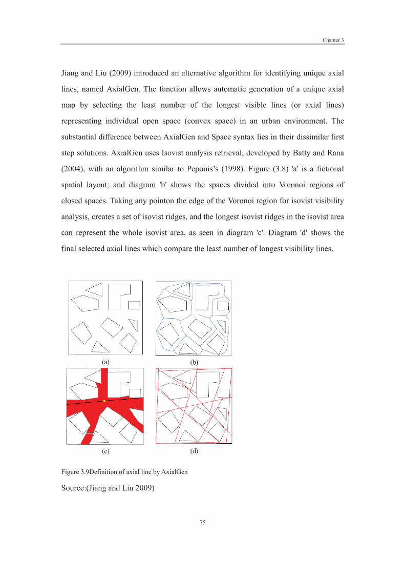
Chapter 3

75

Jiang and Liu (2009) introduced an alternative algorithm for identifying unique axial

lines, named AxialGen. The function allows automatic generation of a unique axial

map by selecting the least number of the longest visible lines (or axial lines)

representing individual open space (convex space) in an urban environment. The

substantial difference between AxialGen and Space syntax lies in their dissimilar first

step solutions. AxialGen uses Isovist analysis retrieval, developed by Batty and Rana

(2004), with an algorithm similar to Peponis’s (1998). Figure (3.8) 'a' is a fictional

spatial layout; and diagram 'b' shows the spaces divided into Voronoi regions of

closed spaces. Taking any pointon the edge of the Voronoi region for isovist visibility

analysis, creates a set of isovist ridges, and the longest isovist ridges in the isovist area

can represent the whole isovist area, as seen in diagram 'c'. Diagram 'd' shows the

final selected axial lines which compare the least number of longest visibility lines.

Figure 3.9Definition of axial line by AxialGen

Source:(Jiang and Liu 2009)

Chapter 3

76

Critics also point out the discussion of necessity of axial lines in space syntax, for

example, Turner (2007) first raised the question “why not other representation?” and

applied an angular segment analysis to compare road-centre line with axial line

models of an urban road network. The results showed that the road-centre line with

angular analysis had a stronger correlation with observed vehicular flows, implying

that it is feasible to combined traditional transportation network analysis

representations with the space syntax method, as it will be convenient to get a

coherent cognition on the movement in the city.

3.6.2 Segment Metric Radius measurement

As Ratti already showed that there is a cross-error in space syntax topology analysis,

when two axial map commutate each other, with the integration value changing

dramatically. The radial segment analysis introduced by Hillierand Penn(2004) can

avoid this error, as the metric radii can control the integration value, which depends

on the size of the analysed area and avoiding edge effects. To do this, firstly, the axial

line map is transformed into a segment line map, breaking down all axial lines by

intersections and removing 25% of the overall length of line. This procedure can be

carried out automatically through the application of the SSX ‘Depthmap’ software.

Rather than topological accessibility, calculating the depth from a segment x to all

other segment, the radii segment analysis for accessibility calculates the depth but

within a fix metric radius (Turner 2007). So, if we know the size of our study area, we

can define the exact radius we need to take so as to avoid edge effects.

Besides space syntax integration, space syntax brings a new notion of ‘choice’, also

known as ‘betweenness’. Betweenness is another centrality measurement popular

used in the field of social network analysis. In space syntax theory, ‘choice’ measures

of the flow through a space (Hillier et al. 1987). It captures how often, on average, a

location may be used in journeys from all places to all others in the city. Locations

Chapter 3

77

that occur on many of the shortest paths between others (i.e., provide a strong choice)

have higher betweenness than those that do not. Normally a main street has a high

value whereas the choice value is a side-street off a main road has a lower volume.

Thus a side street may have high integration but low choice.

3.6.3 Angular segmentmeasurement

Angular segment analysis deals with discontinuities, when geometric configuration

changes slightly. Dalton (2003) argued with her British library hypothesis that people

prefer to minimize the angular distance to their destination.

Source:(Turner 2007)

Figure (3.10) shows a simplified segmented axial map and its associated `j- graph' of

segments. Firstly, to calculate the depth to any location by lowest angular cost, we

calculate the total angular turn from one segment to another segment via the shortest

angular route , (x; y), where x is the starting segment and y the end segment of the

path. Hillier and Iida's method (2005) assign a value in the range of 0 (no turn) to 2

(180°turn) for each turn. So, in figure (3.10), the depth from segment P to segment Q

Chapter 3

78

is 0.5 (a turn of 45°) and the depth to segment R is 1.333 (a turn of 45°followed by a

turn of 60°, note that the direction of turn is immaterial, the turn angle is always

positive).

By introducing alternative measures of distance: shortest path (metric), least angle

change (geometric), and fewest turns (topological), to segments within any fix radius,

with radius measured on metric, geometric and topological domains, space syntax

methodology has become a more accurate and flexible tool for exploring a broad

range of behaviour in the built environment.

3.7 How urban morphology interacts with social

economics phenomenon

Although it emerged from architectural roots Space syntax can be classified as a

location-based social network analysis method. It abstract the spatial accessibility

from a complex urban configuration, describing how one street segment connects to

others and produces indices that can be taken as a surrogate for distribution of

people’s movement within the urban layout. It is known that people have an innate

ability to read or comprehend the meanings of different arrangements or layout of

space, and react to physical infrastructure change (Hillier and Hanson 1984). However,

traditional social economic and environmental studies ignore the spatial information

contained in urban morphology, mainly considering people’s tendency to seek

accessibility for maximum benefits with minimum cost (e.g. distance, travel time,

composite travel cost), as in traditional traffic models. Recently, some studies have

connected space syntax to other academic fields, examining how the spatial

accessibility contained in urban morphology impacts economic and social activities.

For example, Vaughan and Penn (2006) used original census data to examine the

relationship between immigrant clustering and street-level settlement patterns for the

Chapter 3

79

19th century Jewish immigrant quarters of Manchester and Leeds. They found there is

strong negative relationship between the density of Jewish inhabitants and space

syntax integration, indicating that Jewish immigrant chose the higher density areas,

but with lower spatial integration streets. They sought opportunity but also sought

refuge in back streets.

Hillier (2004) addresses the controversy about the relationship between crime and

spatial design, finding a strong correlation between layout type and all kinds of crime.

Traditional street patterns were found to be the best and the most ‘modern’

hierarchical layouts the worst, which indicate that rich and poor alike benefit from

living in traditional streets. He also offers some simple design guidance: enhancing

the accessibility and visibility of public space can positively influence crime rates.

Nevertheless, the research draws a critical lesson that if security is to be enhanced,

both global and local factors must be appropriate, otherwise, the security could not be

increased. This illustrates one of the great strength of space syntax and related

methods: the ability to examine what urban morphology effects at multiple scales

(using multiple radii).

Nes and Rueb (2009) examine how the spatial layout of neighborhoods affect

dwellers’ behavior. They compared four different types of dwelling areas one with

large social problems (Ondiep in Utrecht) and one without (Hof van Delft in

Delft).Two other post-War urban areas were chosen - one with serious social problems

(Oosterwei in Gouda) and one without (Ommoord in Rotterdam). They found that

accessibility is highly related to anti-social behavior problems with a negative sign,

indicating streets with high degree of inter-visibility and adjacent to main routes can

contribute to create safe and vital dwelling areas.

Croxford et al. (1996) examine the relationship between street grid configuration and

vehicular pollution, including Carbon Monoxide (CO), temperature, relative humidity,

Chapter 3

80

light level, and wind speed at six minute intervals. Finally, their research suggested

that the relationship is strong, and urban pollution level could vary cross streets, even

streets spatially close can have very different levels of pollution.

Barros et al. (2009) discuss the potential of space syntax as a tool for estimating

traffic routes. In route analysis, space syntax achieved refined results when compared

to SATURN (Simulation and Assignment of Traffic to Urban Road Networks). The

results showed that the dual approach measuring the movement has better fitness than

the regular geometrical approach, thence, it would be better suited in the transport

field.

Other researchers have connected space syntax to the land value field, exploring the

relationship between urban configuration and land use or housing price. For example,

Brown (1999) noted that real estate analysts found local urban configuration land

design to be important for the field of real estate but that they have not had the tools to

build a strong theory. He compared two different types of shopping mall configuration

using space syntax, and found that the reason why shopping mall number one was

successful while shopping mall number two had failed was mainly due to

configuration design.

Min et al. (2007) explored the relationship between the characteristics of location and

land use, by a case study in Seoul. Their research showed that space syntax

integration value has a high correlation with land value and the location propensity of

industries. Similar findings are also found in the work of Kim and Sohn (2002).

These studies only focus on identifying positive or negative correlations between

urban morphology and social economics activities, which can not be employed for

prediction. Desyllas (2000) explored the relationship between urban street

configuration and office rent patterns in Berlin by multiple regression analysis. A

Chapter 3

81

number of spatial and non-spatial independent variables (e.g. pre-letting time, unit

floor space size and indexes and multipliers) were used in the determination of rent in

his research. The results showed a shift in the pattern of location rent within the short

period under analysis. Whereas the Western CBD was the peak area of location rents

in1991-1994, the pattern by 1995-97 had shifted to Mitte. This was offered as direct

evidence that prime location rents have reorganized around the new spatial structure

of the city revealed by the measure of space syntax global integration. His finding is

supported of the idea that spatial integration has an explanatory value for office rent.

Chiaradia et al. (2009) examine the relationship between street layout and residential

property value by space syntax segment measurement (integration and choice).

Their study applied Council Tax Band as a proxy for residential property value, and

considered other attributes, including non-residential land uses (mainly retail),

property size, building centered density, and age. Their findings showed that

integration is much stronger than choice value, and integration is strongly and

positively related to higher tax bands. When property size, age, and building ambient

density are added, space syntax spatial locational variables are slightly weakened but

still contribute to the property value. The likely reason is that betweeness has a high

variance within a tax band while closeness tends to be more homogenous across

locally continuous roads.

Matthews and Turnbull (2007) examined how street layout affects property value

using space syntax network analysis for both east and west lake Washington. They

used two methods to measure street layout indices: space syntax integration and ratio

of segments/intersections. They found integration to be significant in both west and

East samples using a 1400 feet walking distance radius, but the coefficient signs are

opposite in the two samples. The ratio of segments/intersections had the same result.

They concluded that the portion of house value contributed by street layout critically

depends upon the context of the surrounding development pattern. Enström and

Chapter 3

82

Netzell (2008) also used space syntax methods in a hedonic price approach to test the

urban street layout impact on commercial office rents in Stockholm. They approached

space syntax integration and found that it showed a positive impact on office rent.

More generally, street layout added additional explanatory power to hedonic models

of office rent levels in a major city.

Several points need to be noted about space syntax use in causal modeling. Firstly,

most studies connecting space syntax to other academic fields apply the space syntax

topology measurement, which has been criticized by Ratii (2004) for inconsistencies.

However, it seems that Ratii exaggerated the critics of space syntax. The main point

of attack for space syntax theory by Ratti is that two quite similar axial maps could

have two distinct results. In that case the inappropriate axial map creation would bias

the analysis results. Indeed, the axial map is unique theoretically, which is proved by

the works of Peponis, Wineman, Bafna, Rashid, Kim (1998), Turner, Penn and Hillier

(2005) and Jiang and Liu (2009). Therefore, it is expected that two axial map should

have two different results even they are similar, as the space interpreted by axial map

is actually ‘syntactically’ different. Furthermore, regarding to the axial map

edge-effect pointed out by Ratii (2004), that phenomenon that ‘cross error’ would

happen in topology measurement, as it is only one dimension. Indeed, considering the

notion of metric, the problem has been addressed (Hillier and Penn, 2004), which also

imply that there is no instrinsical inconsistency of topology measurement for axial

map, but it seems difficult to interpret in different urban system with a certain

people’s social activities. Therefore, metric segment and geometric analysis seems

more advanced, as different metric radii could interpret different kind of interactions

between built environment and social processes.

Secondly, correlation is not prediction, so space syntax should be supported by

statistical data, accounting for other attributes in urban system, such as land-use, the

composition of the population, the location of houses and hobs and services and so on

Chapter 3

83

(Ratti 2004). For example, location theory suggests that accessibility could be the

most important determinant of land value or property value. Although there is strong

correlation of urban form and property value, few studies address the question of

whether urban from can be treated as a determinant of property value statistically.

Thirdly, the theory have not outline clearly whether the relationship between building

environment and human societies could vary cross space or different culture context.

However, there is broadly a cognition of spatial heterogeneity of human activities

(Collinge 1996; Monn 2001).

3.8 Summary

In this chapter, I have briefly reviewed space syntax methodology, which is dual

approachto network analysis, measuring the accessibility information contained in a

model of urban morphology. Although some researchers have pointed to

inconsistencies inits topological distance measurement, a series of improvement such

as metric segment analysis and geometric angular cost segment analysis.

As such, these researches will approach the geometric angular segment analysis

measurement of space syntax. The reasons for choosing this measurement are that as

mentioned above, there are some inconsistencies for typology distance measurement,

and metric segment analysis does not consider depth ‘cost’ between two axial lines

according to their angle of incidence. Hillier and Iida (2005) found that angular

segment analysis is efficient and robust for measuring pedestrian movement in a large

area of London. In a city-wide level, both vehicular and pedestrian, users are assumed

to be sensitive of the cost of angular of street layout, and making 135° turn seems cost

more than making 90° turn. Furthermore, in these studies, I adopt Turner’s suggestion

(2007) on creating the axial map based on road central line. The space syntax axial

map was created as follows:

Chapter 3

84

1. A vector urban road network map was prepared and imported into Mapinfo 9.5.

2. An axial line map was created based on the principle of road central lines.

3. The map was modified to take into account of connections in 2D that do not hold

in 3D (for example ‘intersections’ involving viaducts and tunnels.)

4. Using confeego 1.0, space syntax accessibility values were calculated for each

segment.

Two essential indices of space syntax will be applied for capturing the accessibility

contained in urban configuration, namely, integration and choice. Their formulas

(Turner 2007) are provided as follows:

Radius integration

Space syntax integration measures to what extent a segment is close to all others

segments along the shortest depths (paths) of the network. Space syntax integration

for a segment i is defined as:

Equation (3.6)

Where

N is the total number of segments in the network,

is the shortest depths between segment i and j.

is the search length though segment i

The integration value commonly measures how well connected or how close one node

is to all other nodes within the search radius. If the integration value is high it means it

has a high spatial accessibility, as it is easier to move from one segment to others.

Integration has been widely been used in urban and regional analysis as a proxy for

the cost of overcoming spatial separation within a network of road segments.

Chapter 3

85

Radius Choice

Space syntax choice is based on the idea that a segment is more central when it is

traversed by a larger number of the shortest paths connecting all couples of segments

in the network, which is defined as(Turner 2007):

Equation (3.7)

Where:

is the number of shortest paths from segment j to k through x,

isthe weighted sigma function

Using a social network analogue, choice is like the kind of prominence of a person

who acts as an intermediary among a large number of other persons. The choice can

demonstrate how movements go through the network within a specific radius, and

many studies have used different scales of choice to simulate movements associated

with different travel modes. Generally, a high value of choice implies high

frequencies of movement passing through the segment, which is expected to have a

negative impact on residential property value.

I believe the new development of space syntax could improve its measurement in

explaining the interaction between urban spatial structure and socio-economic

activities.

In addition, I have also reviewed the studies that connect space syntax to other social

science fields, especially land value theory. Location is considered as an essential

determinant of housing price distribution, but currently most researchers ignore the

spatial information hidden in an urban street grid. Given that a number of researchers

in the space syntax community have confirmed that there is a high correlation

Chapter 3

86

between urban morphology and housing price pattern, there would seem to be a

fruitful research agenda explaining this further. Hence, in the next chapters, I explore

both the static and dynamic relationship between urban morphology and housing

price,supported by statistical data that accounts for other attributes in urban system.

Specifically, I will look at (a) the basic relationship urban morphological measures of

accessibility and house price, holding other price determinants statistically constant;

(b) the use of space syntax in delineating housing market areas; and (c) the dynamic

relationship between changes in systemic accessibility (through incremental network

improvements) and house price.

Chapter 4

87

Chapter Four:

Urban configuration and housing price

4.1 Introduction

House price can be thought of as a buyer’s evaluation of a bundle of intrinsic and

extrinsic attributes of a housing unit, including structural, locational, neighborhood

and environment attributes (Freeman III 1979a). Many researchers have examined the

contribution to house price of specific sets of factors. Structural characteristics

typicaly include building type, numbers of bedrooms, numbers of bathrooms, garden,

heating, swimming pool and so on (Follain and Jimenez 1985; Sirmans et al. 2005).

Locational variables attempt to model accessibility to various sources of either

positive or negative externalities, such as distance to CBD, local commercial centres,

parks and pollution sources. Environmental characteristics have included air quality

(Freeman III 1979) and noise pollution (Bateman and Executive 2001; Day et al.

2007), and distance to the open space (Bolitzer and Netusil 2000). Neighborhood

characteristics (a subset of locational attributes) typically include quality of school

(Dubin and Goodman 1982; Haurin and Brasington 1996; Downes and Zabel 2002;

Debrezion et al. 2006), socio-economic and racial composition (King and

Mieszkowski 1973; Harris 1999; Ioannides 2002).

Locational attributes are well known to be key determinants of price since they are not

easy to change – generally much less so than structural attributes of a building. In

early studies, many researchers used the monocentric urban bid rent model to

structure their enquiry. In the monocentric model, accessibility to CBD is the major

determinant of location-specific land values and site rents. Many theoretical and

empirical studies are premised on the central idea of the “access-space-trade-off”

model, which gives rise to house prices falling with increased distance from the city

Chapter 4

88

center (Alonso 1964; Muth 1969; Mills 1972). These early studies are considered

seminal in urban theory building but have given way to more nuanced studies that

better capture the multicentric and network geometry and topology of locational

advantage (McDonald 1987). A variety of accessibility measuring devices has been

adopted to capture the locational premium effect more sensitively than the purely

Euclidean distance used in many studies on property value (Niedercorn and Ammari

1987; Hoch and Waddell 1993). Specific approaches include studies specifying

accessibility index by travel time (Landau et al. 1981), job accessibility (Srour et al.

2002), railway infrastructure improvement (Henneberry 1998), and systemic street

network connectivity (Matthews and Turnbull 2007; Enström and Netzell 2008).

In this chapter, I explore the intuitive hypothesis that important information about

urban agglomeration externalities is contained in the urban street network grid and

can be captured from accessibility indicators measured from a topological network

model of the grid. Most hedonic models fail to take note of essential spatial

information in the street layout: network connectivity, network distance, angular

distance and so on, which in turn, have been shown to have a strong influence on

pedestrian behavior, congestion and other influences on house price (Hillier and

Hanson 1984b; Hillier 1996; Penn et al. 1998; Vaughan et al. 2005; Chiaradia et al.

2009).

I test this hypothesis using Cardiff as the study area. A model of a sub-section of the

Cardiff street grid was modeled using the space syntax methodology and various

measurements of network accessibility were taken from the model to form additional

locational variables in a hedonic model of house prices. Furthermore, Garrett (2003)

state the economic behavior depends upon the level of data aggregation, that is why

the sign and significance of coefficient estimates from the regression using aggregated

data differ from regressions using less aggregated data. In doing this I consider two

level data aggregation, one is disaggregated data level, the other is aggregated by

Chapter 4

89

output area level, testing the following set of specific hypotheses:

1. Accessibility information derived from a topological network model improves

hedonic model performance, compared to other locational data, in respect of:

a. % of variation explained

b. distinguishing between positive and negative impacts of accessibility

c. spatial auto-correlation issues

2. The advantages hypothesized in (1) hold with both aggregate and disaggregate

models

3. The explanatory power of network accessibility metrics varies with the shape of

the study area.

In Section 2, I review previously published work relating to these issue. The hedonic

model is presented in Section 3. The region and data are described in Section 4.

Results are presented in Section 5, where we run 6 types of model: Model I (a) is a

disaggregated hedonic model with conventional locational variables; Model I (b) is a

disaggregated model with a full set of network accessibility variables (space syntax

Integration and Choice measured at various radial scales in network space). Models

I(c) is a set of 14 models each with a single pair of Integration and Choice measure,

calculated at a particular radial scale in order to compare the efficacy of different

scales of measurement. Models II (a), (b) and (c) are the same but using data

aggregated to Census output areas rather than individual house units. Section 6

summarizes the findings and concludes.

4.2 Locational information in hedonic models

In access versus space trade-off models, transportation costs are traded off against

land rents. Improvements in transportation infrastructure are assumed to reduce

commuting costs via savings in commuting time, releasing more from a household

budget to spend on land rent (Alonso 1964b; Muth 1969; Mills 1972). However,

Chapter 4

90

Alonso’s (1964) monocentric model is clearly one pertaining to a particular historical

phase in a city’s evolution and does not adequately capture accessibility value where

workplaces are not solely located in the city center(McDonald 1987), and where trips

to work form a declining share of overall household travel. The polycentric nature of

many housing-market areas makes one-dimensional separation measures like physical

distance and travel time from a distinctly defined center problematic. The presence of

multiple-worker households and multiple workplaces motivated the search for

alternative separation measures, as Heikkila et al note:

``with multiple-worker households, multiple workplaces are common; given a high

degree of residential mobility, sites offering accessibility to many employment nodes

are more valuable because it is not very likely that successive owners will work in the

same workplace'' (1989, page 222).

The study by Heikkila et al found that distance to CBD had a very low t-value and an

unexpected sign in a house price hedonic model of Los Angeles in 1980 and they

concluded that the impact of workplace accessibility has been overemphasized.

Richardson et al. (1990)note that the effect of distance to CBD may have declined,

find in that the distance coefficient for Los Angeles CBD was significantly negative in

a dataset for 1970. Waddell et al. (1993) emphasized the importance of including

distance to secondary employment centers, and found both a strong and significant

asymmetric CBD-gradient and strong local effects from non-CBD employment

centers. More recently McMillen (2003)took an alternative repeat sales model to

identify changes in housing price distance gradients for Chicago CBD and found the

distance coefficients of Chicago CBD was insignificant in the early to mid 1980s, but

that this situation had reversed by the 1990s. Orford (2002) specified a multilevel

hedonic model to evaluate locational externalities, examining a range of locational

effects on house prices. In terms of property-level externalities, he used distance to

CBD, motorway exits, railway stations, shopping centers, and suburban employment

Chapter 4

91

centers. He also considered proximity to nonresidential land uses such as parks,

schools, industry, commercial, local shops, recreational centers and cultural and

educational centers. His results showed a complex geography of locational externality

effects, with areas of positive and negative externalities in juxtaposition across highly

localised areas.

There have been detailed studies of transport behavior and house price, for example,

Tang (1975)which showed that savings in transportation cost tend to have a positive

and significant impact on house prices in line with Alonso-style trade-off models. In

general, the impacts of transportation on residential markets are related to availability

of transport; transportation costs; travel time; and convenience of transport. Gibbons

and Machin (2005) explored the effects on house prices of a transport innovation for

households in London in the late20th century. They defined rail access in two ways:

distance to a station and service frequency at the nearest station. Distance changes

induced by the transport innovation were associated with price changes and the price

effect was large compared to the monetary valuation of other local amenities. On the

other hand, Adair et al. (2000)examined the relationship of housing price and

accessibility in Belfast urban area. They adopted a traffic gravity model, calculating

the accessibility index for locations to various opportunities by different types of

vehicle, finding that the index was significant, but accounts for a very small percent of

the variation in house prices. Specific physical housing attributes and socioeconomic

variables appeared to be a lot more influential. An example of a more sophisticated

accessibility index is found in Osland and Thorsen(2008), who utilized a hedonic

model to confirm that gravity-based labor-market accessibility significantly

contributes to housing prices. Significantly, he found that labor-market accessibility is

not an adequate alternative to distance from the CBD; illustrating that there are

multiple attributes bundled into the concepts of accessibility. Webster notes the

conventional distinction between general and specific accessibility, elaborating this

into the idea of geometric (or topological) accessibility and economic accessibility

Chapter 4

92

and giving both explicit economic interpretations (Webster 2010).

Grid structure (street layout) is an attribute of a city that influences both general and

special accessibility. It confers general demand potential by virtue of the number of

people passing through a location and it confers specific demand potential by virtue of

the locational configuration demands of specific land uses. Matthews and Turnbull

(2007) examined how street layout affects property value using space syntax network

analysis for both east and west lake Washington. They used two methods to measure

street layout indices: space syntax integration (defined formally in the next section of

this paper) and ratio of segments/intersections. They found integration to be

significant in both west and East samples using a 1400 feet walking distance radius,

but the coefficient signs are opposite in the two samples. The ratio of

segments/intersections had same result. They concluded that the portion of house

value contributed by street layout critically depends upon the context of the

surrounding development pattern. Enström and Netzell (2008) also used space syntax

methods in a hedonic price approach to test the urban street layout impact on

commercial office rents in Stockholm. They calculated space syntax integration and

found that it had a positive impact on office rent. More generally, street layout added

additional explanatory power to hedonic models of office rent levels in a major city.

The accessibility information contained in an urban street layout model would seem,

in principle, a suitable approach for measuring locational characteristics at a

disaggregated level without a pre-defined map of or knowledge about attractiveness

hot spots. This chapter explores this proposition that whether urban morphology has

impact on housing price.

4.3 Methodology

Space syntax is a set of analytical tool for quantatifying and describing the interaction

between human and building environment (Hillier and Hanson 1984). Space syntax

Chapter 4

93

measures the accessibility of urban street and building configuration, initially based

on the assumption that people move to areas where they can see, describing how the

street network is connected (Hillier et al. 1993b). As discussed in Chapter three, one

substantive difference between space syntax and traditional geographic network

analysis, is that space syntax is a dual approach, which identifies streets as nodes and

intersections as links (Batty 2004).

I adopt the segment metric radii measurement of space syntax. for this study,

considering Turner’s suggestion (2007) creating the axial map based on road central

line. The overall methodology involves (a), creating an axial line map of a portion of

the city of Cardiff grid; (b) calculating space syntax spatial accessibility indicators for

each section in the grid, using the ‘Confeego’ software (www.spacesyntax.org);

(c)compiling house price data for the same area and linking it to grid sections; (d)

selecting a hedonic model functional form; (e) organizing the data for regression; (f)

conducting econometric tests, predicting house price on the basis of, inter alia,

connectivity information derived from the network model. These steps are elaborated

below.

4.3.1 Space syntax spatial accessibility index

Two important measures of spatial accessibility: (a)integration, also known as

closeness, and (b) choice, used in this study have been described already in Chapter

three.

In this study, I will measure integration and choice at different radius: 400m, 800m

1200m, 1600m, 2000m, 2500m, 3000m, 4000m, 5000m, 6000m, 7000m, 8000m,

10000m and global Nm (the entire city grid model). From published research, these

can be associated with different uses of the grid, for example, 400m -1200m is

walking scale and 1600m-2000m is cycling or running scale, while above 2500m is

Chapter 4

94

automobile scale. Choice of radius also depends on the area of study. Larger study

areas obviously require a wider range of radius. Through testing the different choice

radii on housing price in out study area, I can imply what kind of grid-use activity can

affect house prices.

4.3.2 Hedonic regression model

The hedonic price model, derived mostly from Lancaster’s (1966) consumer theory

and Rosen’s (1974) model, posits that a property possesses a myriad of attributes that

combine to form bundles of utility-affecting attributes for consumers. The implicit

price of the housing attribute revealed in the regression coefficient is equal to people’s

willingness to pay for each individual characteristic. The price of the house then, is

the sum of the implicit prices for the attributes that are contained in it. Thus, the

hedonic price approach enables the possible influence of each of the many attributes

on the house price to be tested and analyzed.

The hedonic price model employed in this study is specified following Orford

(1999)’s work, exploring the locational externality for Cardiff housing market:

Where,

= Transaction price of residential property ;

= floor area;

D = straight Distance to the city center;

Chapter 4

95

= accessibility of urban configuration: integration and choice at different radius;

DU_N =dummy variable for new building;

DU_D =dummy variable for detached house,

DU_SE = dummy variable for semidetached house;

DU_T = dummy variable for terrace house;

DU_Te = dummy variable for tenure;

DU_BC = dummy variable for people live in blue collar communities;

DU_CL = dummy variable for people live in the city;

DU_PS = dummy variable for people are prospering suburbs;

DU_CC = dummy variable for people are constrained by circumstances;

DU_TT = dummy variable for people are typical traits;

Y2000 = dummy variable for transaction year of property in 2000;








= A random error, which expected to be normal distribution with a mean of zero as

well as the variance of

4.4 Data and study area

4.4.1 Datasets

The dataset employed in this study mainly consists of three parts. The spatial data on

housing price and all structure characteristics, which comes from the land registry;

socioeconomic status information from the 2001 census data; and urban configuration

Chapter 4

96

information from a space syntax model based on data from the latest UK ordnance

survey (http://edina.ac.uk/digimap/).

Housing price and all structural characteristics are collected by the Land Registry on

behalf of the UK government. The land registry department holds details of title,

covenants, plot details for residential and commercial property in England and Wales

since 1995. Purchasing the dataset from the registry, gives access to a service license

to use the following data: the full address of the property (PAON, SAON, street,

postcode, locality, town district, country), property size, transaction price for the

property, date of transfer, property type (Detached, Semi, Terraced, Flat/ Maisonett),

whether the property is new build or not, and whether the property is freehold or

leasehold. In this study, the dataset has 16,867 transactions during a period 2001 to

2007 at building level. Compared with previous studies of Cardiff housing markets

his is a large study, with Orford (1999) using 1500 transactions (using asking price

from the estate agents). The dataset also includes data for dwelling type, gross internal

floor area, numbers of bathrooms, numbers of bedrooms, central heating, age bands,

and off street parking.

Neighborhood type variables in this study, the Grand Index will be used to

demonstrate the socio-economic status of the output area, which is from the 2001

Census data (http://edina.ac.uk/ukborders/). According to the Output Area

Classification (OAC), the Grand index is divided into seven groups: blue collar

communities, city living, countryside, prospering suburbs constrained by

circumstances, typical traits and multicultural.

Urban configuration data are derived from the Ordnance Survey, which is the national

mapping agency of Great Britain, which provides accurate and up-to-date

geographical data. This kind of data cannot be implemented directly in space syntax

network analysis as the space syntax method requires a model of the urban street

Chapter 4

97

segments network based upon the axial line, which is drawn based on the road central

line. Furthermore, the area for network analysis should be bigger than the study area,

normally an extra 3000m. Pre-processing also needs to convert three-dimensional

intersections like viaducts or tunnels into a syntax model. Having prepared the OS

data in this way, confeego 1.0 (www.spacesyntax.org) was used to calculate the urban

configuration spatial accessibility, generating accessibility indices for each segment.

The three datasets were combined through ArcMap. The straight line distance of each

property to the city centre was also calculated, and segment accessibility values were

attached as an attribute to each house based on nearest criteria.

4.4.2 Study area

Since the object of the study is to examine whether the accessibility of urban

configuration grid impact on the housing price, I selected a test area suitable for our

experiment. The selection was constraint by the dataset available. Cardiff is the

capital of Wales, the largest city and with the highest population in Wales. According

to recent estimates, the population of the unitary authority area is 324,800m2. Orford

(2000) points out that the housing submarkets of Cardiff are stratified by dwelling

type, based upon 26 basic units or communities used by the city council for

administrative purpose.

Chapter 4

98

Source: author

The study area is limited to the eastern inner city wards of Cardiff which amount to

almost including 11 wards: Cathays, Heath, Llanishan, Cyncoed, Penylan,

Plasnewydd, Pentwyn, Llannumney, Rumney, Splott and Adamstown. The following

table (4.1) illustrates the number of properties which meet the criteria of this study:

Pentyrch

Trowbridge

Splott

Lisvane

Ely

Creigiau/St. Fagans

Butetown

Radyr

Rhiwbina

Heath

Llanishen

Rumney

Grangetown

Cyncoed Pentwyn

Penylan

Canton

Caerau

Cathays

FairwaterLlandaff

Pontprennau/Old St. Mellons

GabalfaLlandaff North

Whitchurch and Tongwynlais

Riverside

Llanrumney

Plasnewydd

Adamsdown

¯

0 2,300 4,6001,150 Meters

Property

Cardiff Wards

Study Area

Chapter 4

99

Year 2000 2001 2002 2003 2004 2005 2006 2007 2008

N 1753 2198 2503 2228 2148 1737 2072 2057 174

Total 16867

From the urban spatial layout perspective, there is a motorway (A48M) which divides

the study area into two sample areas that differ greatly. They display significantly

different social and development characteristics. The northern part of the study area is

predominantly inhabited by family households and households who have access to

private motor vehicles. The second sample area has high levels of residents who are

students and are mainly depending on public transportation and walking. So based on

this finding from the mapping, we can pre-define two spatial provisions: the northern

and the southern part. It can be noted that earlier spatial approaches to housing market

subdivision might have used this structure on its own.

For the aggregated hedonic models, the unit of measurement is output area, there

being 322 census output areas in our study area. Figure 4.2 describes the average

housing price at the aggregated level displayed in output areas.

Chapter 4

100

Source: author

List of variables

Splott

Lisvane

Butetown

Trowbridge

Llanishen

Heath

Rumney

Cyncoed Pentwyn

Penylan

Cathays

Grangetown

Pontprennau/Old St. Mellons

Riverside

Llanrumney

Canton

Gabalfa

Rhiwbina

Plasnewydd

Adamsdown

Llandaff North

Whitchurch and Tongwynlais

Llandaff

Llandaff

¯

0 920 1,840460 Meters

Ave_PRICE

< -1.5 Std. Dev.

-1.5 - -.50 Std. Dev.

-.50 - .50 Std. Dev.

.50 - 1.5 Std. Dev.

1.5 - 2.5 Std. Dev.

> 2.5 Std. Dev.

Wales OA

Chapter 4

101

Fifty-five variables were prepared for the hedonic models: 21 dummy variables and

24 continuous variables.

Variables S L N E SSX T Type Description 1. LN_FL Continuous Ln floor area 2. DU_N Dummy New building (Yes=1 No=0)

3. DU_D Dummy Detached House (Yes=1 No=0)

4. DU_SE Dummy Semidetached House Yes=1 No=0

5. DU_T Dummy Terrace house Yes=1 No=0

6. DU_F Dummy Flat Yes=1 No=0

7. DU_TE Dummy Tenure Freehold=1 Lease=0

8. DU_BC Dummy Blue collar communities Yes=1 No=0

9. DU_CL Dummy Lliving in the city Yes=1 No=0

10. DU_PS Dummy Prosperious suburbs Yes=1 No=0

11. DU_CC Dummy Constrained by Circumstances Yes=1 No=0

12. DU_TT Dummy Typical traits Yes=1 No=0

13. DU_MU Dummy Multicultural Yes=1 No=0

14. LN_D Continues straight-linedistance to CBD

15. LN_D1 Continuous straight line distance to Cardiff bay

16. LN_D2 Continuous straightline distance to Lake

17. LN_D3 Continuous straight line distance to hospital

18. LN_D4 Continuous straightline distance to Bute Park

19. Y2000 Dummy

20. Y2001 Dummy

21. Y2002 Dummy

22. Y2003 Dummy

23. Y2004 Dummy

24. Y2005 Dummy

25. Y2006 Dummy

26. Y2007 Dummy

27. Y2008 Dummy

28. CH_R400M Continuous SSX choice value at radius 400m













41. LOG_CH Continuous SSX choice value at radius m

Chapter 4

102

42. INT_R400M Continuous SSX integration value at radius 400m













55. INT Continuous SSX integration value at radius m

4.5 Empirical results

4.5.1 Street network analysis

Finally, there are a total of 28 space syntax variables with 14 different search radii

employed for testing the relationship between urban morphology and housing price,

and their visualized maps are in Appendix -4. Generally, the red color in integration

represents high connectivity, and the axial line with blue color indicate the

connectivity of this street segment is low. With respect to the visualized choice maps,

the high traffic flows is in red and segregated segments are colored with blue. It is

noted that with the search radii increasing, the effect areas are enlarged, and geometry

polycentric came out, shifted and regrouped which are found in both integration and

choice maps. Furthermore, it is surprising to find that within a local level, the highest

integration value is located in two streets, namely Crwys road – Albany road and

Cowbridge east road, where are numbers of retail and commercial shops (Figure A4.1,

2, 3, 4, 9 and 10). However, when the search radii are above 3 km, the highest

integration value are shifted to the motorway (A48), shown in Figure A4.11, 12, 17,

18, 19 and 20. This implies that the travel preference of pedestrian and automobile on

urban form are different, and it indicates maybe around 3 km is the optimal scale for

all the people.

Chapter 4

103

4.5.2 Disaggregated data

I first explore the relationship between urban layout and house price at a

disaggregated level. The descriptive statistics of the variables are shown in table 4.3.

There are 16297 valid observations; 92% buildings are not newly built; 79% of

properties are freehold; terraced houses make up the largest portion at 52%; and flats,

the second largest portion. Only 5% of the output areas in the study are in the

‘constrained by circumstances’ neighborhood class; in contrast, 28% of output areas

in the study area are in the ‘typical traits’ class. There are equal numbers of housing

transactions from 2000 to 2007.

N Minimum Maximum Mean Std. Deviation

LN_PRICE 17207 9.210 14.039 11.680 0.567

LN_FL 16297 1.793 9.595 4.903 1.071

LN_D 17207 12.804 12.821 12.811 0.004

LN_D1 17207 12.804 12.821 12.811 0.004

LN_D2 17207 12.804 12.821 12.811 0.004

LN_D3 17207 12.804 12.821 12.811 0.004

LN_D4 17207 12.804 12.821 12.811 0.004

DU_N 17207 0.000 1.000 0.080 0.268

DU_D 17207 0.000 1.000 0.100 0.300

DU_SE 17207 0.000 1.000 0.210 0.407

DU_T 17207 0.000 1.000 0.520 0.500

DU_F 17207 0.000 1.000 0.170 0.375

DU_TE 17207 0.000 1.000 0.790 0.411

DU_BC 17207 0.000 1.000 0.110 0.310

DU_CL 17207 0.000 1.000 0.270 0.446

DU_PS 17207 0.000 1.000 0.150 0.354

DU_CC 17207 0.000 1.000 0.050 0.208

DU_TT 17207 0.000 1.000 0.280 0.449

DU_MU 17207 0.000 1.000 0.150 0.353

Y2000 17207 0.000 1.000 0.110 0.309

Y2001 17207 0.000 1.000 0.130 0.340

Y2002 17207 0.000 1.000 0.150 0.359

Chapter 4

104

Y2003 17207 0.000 1.000 0.130 0.339

Y2004 17207 0.000 1.000 0.130 0.332

Y2005 17207 0.000 1.000 0.100 0.301

Y2006 17207 0.000 1.000 0.120 0.328

Y2007 17207 0.000 1.000 0.120 0.321

Y2008 17207 0.000 1.000 0.010 0.099

CH_400M 17207 0.000 3.183 1.483 0.923

INT_400M 17207 0.000 95.898 29.479 16.135

CH_800M 17207 0.000 3.879 2.152 1.277

INT_800M 17207 0.000 194.551 68.402 40.154

CH_1200M 17207 0.000 4.464 2.510 1.485

INT_1200M 17207 11.928 350.988 120.269 67.933

CH_1600M 17207 0.000 4.961 2.745 1.626

INT_1600M 17207 16.489 482.002 181.727 97.358

CH_2000M 17207 0.000 5.287 2.912 1.721

INT_2000M 17207 26.903 576.524 246.244 125.338

CH_2500M 17207 0.000 5.570 3.069 1.817

INT_2500M 17207 30.971 719.865 327.692 155.646

CH_3000M 17207 0.000 5.789 3.195 1.891

INT_3000M 17207 44.303 825.042 411.021 181.137

CH_4000M 17207 0.000 6.155 3.389 2.004

INT_4000M 17207 77.035 1044.480 584.539 219.047

CH_5000M 17207 0.000 6.430 3.529 2.091

INT_5000M 17207 141.572 1317.720 763.448 254.955

CH_6000M 17207 0.000 6.655 3.634 2.161

INT_6000M 17207 251.813 1604.220 944.528 281.435

CH_7000M 17207 0.000 6.887 3.719 2.209

INT_7000M 17207 359.996 1793.710 1114.311 298.407

CH_8000M 17207 0.000 7.058 3.778 2.249

INT_8000M 17207 441.707 1939.790 1248.791 308.140

CH_10000M 17207 0.000 7.273 3.834 2.295

INT_10000M 17207 616.409 2107.210 1412.711 292.122

LOG_CH 17207 0.000 7.567 3.834 2.337

INT 17207 858.122 2150.760 1521.650 245.688

Valid N (listwise) 16297

Two models were run: with and without the spatial accessibility indicators. To specify

the latter model, a correlation test was undertaken (Annex One), which found that all

locational variables and environmental variables such as the distance to the CBD and

distance to the major park, are highly correlated. This is probably due to the scale of

the research area, which is small, I therefore decided to only consider the locational

Chapter 4

105

attributes: straight distance to the city center. Dummies were created by suppressing

“flat” and “multicultural” categories of the respective house-type and socioeconomic

neighborhood type variables.

Model I (a) uses the traditional hedonic variables including structure, neighbourhood,

environmental variables and year of sale attributes (Table 4.4)

The adjusted R-square is 0.615. The log likelihood is minus 6184.150, the Akaie info

criterion is 0.761631, F is 1241.266, and the probability of the F-test is 0.000. I

conclude that the model fits the data well and that each independent variable is

significantly linear. As we expect, distance to the CBD has a negative relationship

with house price; ‘blue collar community’ is also negatively related to the house price.

All independent variables have a significant effect on housing price at a 5%

confidence level, with all VIFs below ten. Model I’s residual “White-test” results

(table 4.5) shows that the N*adjust R-square is bigger than Chi-square (21), indicating

heteroscedasticity, so the prediction of the model is poor. Moran’s I (table 4.6) is

0.239, with a Z-score of 87.986 (P=-0.000) and there exist a significantly positive

correlation, indicating the presence of a high value housing cluster and a low value

housing cluster. I can imply the coefficients of each attributes are unreliable, leading

to over estimation.

Model I (b) includes all 28 space syntax spatial accessibility variables (Table 4.4). The

adjusted R-square is 0.654 and the log likelihood is -5303.758. The Akaike info

criterion is 0.657 and the F-value is 642.632. Variation explained thus increased by

6.4% and the log likelihood increased by 14.23%. Additionally, the Akaike info

criterion rose by 13.75% and the sum of squared residuals decreased by

10.24%.Model I (b) with urban configuration information therefore has higher

explanatory power than model I (a). All variables in model I (b) are significant except

DU_BC (‘Blue collar neighbourhood’). This may be because Blue collar class people

are more sensitive to accessibility. Distance to CBD has become positive, but with a

Chapter 4

106

weak standardized coefficient (0.081). This suggests that once systemic network

accessibility is accounted for, distance to CBD becomes a marginal influence,

exerting a negative effect by virtue of the congestion associated with it. All variables

in model I(a) have larger VIFs than in model I(b) but are still under 10, indicating that

there is some interaction between physical attributes, socioeconomic attributes and

locational attributes, e.g. higher income people purchase larger houses farther from

the city center but with high accessibility. Some of the network accessibility variables

have positive coefficients and others negative, with similar P-values for all. As

expected, most VIFs for the accessibility variables are over 10, indicating strong

multicolinearity in model I(b). As discussed, the multicoliniarity will not affect the

model’s accuracy of prognosis, but the coefficients and the sign of coefficients should

not be considered reliable. The White test for model I (b) (table 4.5) shows that

N*adjust R-square > Chi square (48), which indicates heteroscedasticity in the

residual. The OLS is no longer the best estimation and the model has lost its ability to

predict. The z score of Moran’s I in model I (b) (table 4.6) is 47.514 (p=0.000), which

tell us there is still positive spatial autocorrelation in the residuals of the model.

However, the z score is smaller than in model I (a), with a 42.59% improvement,

indicating that the space syntax variables ease the spatial autocorrelation effect and

they add extra information in differentiating variation between the sample house price

values.

Notwithstanding the slight reduction in some aspects of the model’s reliability, it is

still possible to conclude that the space syntax spatial accessibility variables have

improved the estimation of house prices. I can say that urban layout significantly

affects housing price and that when the configuration effect of the urban grid is taken

into account, other cruder measures of accessibility (distance to CBD) are shown to

have weaker and counter intuitive effects on price.

Chapter 4

107

Model I(a) Model I(b)

Adjusted R-squared 0.615 Adjusted R-squared 0.654

Akaike info criterion 0.762 Akaike info criterion 0.657

Log likelihood -6184.150 Log likelihood -5303.758

F-statistic 1241.266 F-statistic 642.632

Coeff. SD. Coef. t Sig. VIF Coeff. SD. Coeff. t Sig. VIF

Constant 449.996 29.911 0.000 -168.279 -6.032 0.000

LN_FL 0.134 0.251 34.096 0.000 2.289 0.128 0.240 31.889 0.000 2.670

LN_D -34.357 -0.200 -29.262 0.000 1.984 13.893 0.081 6.381 0.000 7.588

DU_N 0.144 0.065 11.147 0.000 1.429 0.126 0.057 9.762 0.000 1.589

DU_D 0.736 0.365 42.239 0.000 3.165 0.724 0.359 43.358 0.000 3.232

DU_SE 0.469 0.335 30.419 0.000 5.123 0.464 0.331 31.363 0.000 5.247

DU_T 0.271 0.237 18.186 0.000 7.200 0.287 0.251 19.931 0.000 7.448

DU_TE 449.996 0.163 18.105 0.000 3.439 0.216 0.156 18.009 0.000 3.522

DU_BC -0.035 -0.019 -2.808 0.005 2.013 -0.004 -0.002 -0.312 0.755 2.369

DU_CL 0.193 0.152 21.145 0.000 2.185 0.121 0.095 12.629 0.000 2.667

DU_PS 0.514 0.302 41.973 0.000 2.199 0.439 0.259 32.582 0.000 2.965

DU_CC 0.079 0.029 4.944 0.000 1.418 0.049 0.018 3.040 0.002 1.604

DU_TT 0.198 0.156 21.471 0.000 2.247 0.124 0.098 12.605 0.000 2.828

Y2001 0.114 0.068 9.999 0.000 1.953 0.114 0.068 10.605 0.000 1.957

Y2002 0.288 0.181 25.930 0.000 2.053 0.294 0.184 27.882 0.000 2.059

Y2003 0.497 0.296 43.494 0.000 1.963 0.505 0.301 46.496 0.000 1.971

Y2004 0.667 0.387 57.596 0.000 1.912 0.678 0.393 61.616 0.000 1.919

Y2005 0.764 0.399 62.184 0.000 1.740 0.775 0.404 66.231 0.000 1.754

Y2006 0.804 0.465 69.396 0.000 1.899 0.798 0.461 72.490 0.000 1.906

Y2007 0.851 0.480 72.289 0.000 1.870 0.848 0.479 75.695 0.000 1.883

Y2008 0.846 0.146 28.831 0.000 1.082 0.854 0.147 30.672 0.000 1.084

CH_400M -0.024 -0.039 -2.046 0.041 17.251

INT_400M -0.002 -0.069 -5.150 0.000 8.400

CH_800M 0.066 0.148 1.944 0.052 272.887

INT_800M -0.001 -0.073 -2.310 0.021 47.311

CH_1200M 0.065 0.169 1.190 0.234 951.596

INT_1200M 0.000 0.022 0.449 0.654 110.491

CH_1600M -0.110 -0.312 -1.734 0.083 1525.000

INT_1600M -0.002 -0.361 -5.344 0.000 214.616

CH_2000M -0.023 -0.070 -0.352 0.725 1881.000

INT_2000M 0.003 0.654 8.889 0.000 254.653

CH_2500M -0.322 -1.024 -3.792 0.000 3434.000

INT_2500M 0.000 0.036 0.448 0.654 310.407

CH_3000M 0.374 1.235 4.936 0.000 2947.000

INT_3000M 0.000 -0.229 -3.010 0.003 273.512

CH_4000M 0.065 0.228 1.032 0.302 2305.000

Chapter 4

108

INT_4000M 0.000 0.116 1.743 0.081 209.872

CH_5000M -0.010 -0.035 -0.118 0.906 4110.000

INT_5000M -0.001 -0.629 -8.875 0.000 236.375

CH_6000M 0.063 0.237 1.014 0.311 2575.000

INT_6000M 0.000 0.081 0.946 0.344 342.870

CH_7000M -0.052 -0.200 -0.800 0.424 2936.000

INT_7000M 0.002 0.909 9.800 0.000 405.171

CH_8000M -0.015 -0.059 -0.220 0.826 3337.000

INT_8000M 0.000 -0.053 -0.661 0.509 299.841

CH_10000M -0.021 -0.084 -0.420 0.674 1880.000

INT_10000M 0.001 0.444 7.866 0.000 150.178

LOG_CH -0.046 -0.188 -3.163 0.002 165.544

INT -0.001 -0.590 -15.176 0.000 71.220

Model I (a) Model I (b)

N=16297 Adjust R-square 0.019 N=16297 Adjust R-square 0.024

N*Adjust R-Square= 317.0412 Chi-square(21)= 32.671 N*Adjust R-Square= 395.968 Chi-square(48)= 65.171

N*Adjust R-Square > Chi-square(21) N*Adjust R-Square > Chi-square(21)

Model I (a) Model I (b)

Moran’s I index: 0.239 Expected Index: -0.000 Moran’s I index: 0.129 Expected Index: -0.000

Variance: 0.000 Z Score: 87.986 Variance: 0.000 Z Score: 47.514

p-value: 0.000 p-value: 0.000

I move on to look at the explanatory power of integration and choice measures at

different radii in order to find out at what spatial scale the space syntax accessibility

measures give most explanation, and it will imply us what kind people’s activities is

most associated with housing price in study area.

Each radius variable was put separately into model I(c). Table4.7 shows the

comparison of T and P values for choice and integration at each spatial scale. VIF

Chapter 4

109

scores for each of the 14 versions of Model I (c) are within the desired range. I

conclude from the table that choice and integration measures are significant whatever

the spatial scale at which they are measured. This suggests that the volume of network

flows and the convenience of connectivity at any point in the urban road network both

significantly affect house price. The fact that all radii are significant suggests either

that they all capture a similar accessibility effect or that they capture scale-specific

effects that substitute for each other.

Choice has a negative relationship and integration a positive relationship with house

price. This is as expected, since choice indicates likelihood of congestion and

integration indicates ease of access to all other places within the radially-curtailed

network section. In this way, the two network metrics neatly differentiate positive and

negative network externalities. More can be said by examining the pattern of T-values.

The change in T-value for integration rises from 2.773 to a peak of 28.163 at a radius

of 7000m and then falls again to 20.556.for a raidally unconstrained model (Figure

3.5). There is also a minor peak between 2000m and 3000m. An opposite trend of

T-values is observed for choice: first decreasing and then starting to rise at -8.374, the

lowest point being reached at radius of 7000m and having a small negative fluctuation

between 2000m and 3000m. The adjusted R square values also peak at 7000m.

I may therefore conclude that for the study area, house prices seem to be most

sensitive to network accessibility metrics measured at a radius of 7000m and that this

is true for negative and positive road network externalities. 7KM is the spatial scale

that people use automobile within 10 15 mins. This indicates peoples’ wiliness to

pay extra only within a 10-15 mins driving distance to anyplace. Walking distance

accessibility (400m-1200m) has less impact on housing price, but may be powerful in

subsamples within smaller areas. Note that with radius increases the explanatory

power of both integration and choice changes systematically, indicating that

empirically, space syntax metric measurement is more accurate than the conventional

Chapter 4

110

geometric locational measurement. Network configuration becomes less influential

beyond the 7000m scale as it extends into ex-urban areas and the parts of the city the

other side of the CBD, which indicates once more that beyond this distance there is no

more city-scale externality effects captured in housing prices. This shows that optimal

radius for measuring network accessibility is related to the size and shape of the study

area.

400M 800M 1200M 1600M 2000M

CH INT CH INT CH INT CH INT CH INT

T -2.314 2.773 -4.627 11.343 -5.98 15.42 -7.332 19.024 -8.536 23.439

Sig. 0.021 0.006 0 0 0 0 0 0 0 0

Ad-R2 0.615 0.618 0.621 0.624 0.628

2500M 3000M 4000M 5000M 6000M


T -8.416 24.836 -8.139 24.609 -7.367 22.2.8 -7.066 21.71 -0.845 25.236

Sig. 0 0 0 0 0 0 0 0 0 0

Ad-R2 0.629 0.629 0.627 0.626 0.63

7000M 8000M 10000M Infinite

CH INT CH INT CH INT CH INT

T -10.04 28.163 -9.801 26.805 -8.487 23.18 -8.374 20.556

Sig. 0 0 0 0 0 0 0 0

Ad-R2 0.633 0.632 0.628 0.625

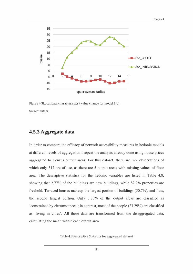
Chapter 4

111

Source: author

4.5.3 Aggregate data

In order to compare the efficacy of network accessibility measures in hedonic models

at different levels of aggregation I repeat the analysis already done using house prices

aggregated to Census output areas. For this dataset, there are 322 observations of

which only 317 are of use, as there are 5 output areas with missing values of floor

area. The descriptive statistics for the hedonic variables are listed in Table 4.8,

showing that 2.77% of the buildings are new buildings, while 82.2% properties are

freehold. Terraced houses makeup the largest portion of buildings (50.7%), and flats,

the second largest portion. Only 3.83% of the output areas are classified as

‘constrained by circumstances’; in contrast, most of the people (23.29%) are classified

as ‘living in cities’. All these data are transformed from the disaggregated data,

calculating the mean within each output area.

15

10

5

0

5

10

15

20

25

30

35

0 2 4 6 8 10 12 14 16

tval

ue

space syntax radius

SSX_CHOICE

SSX_INTEGRATION

Chapter 4

112

N Minimum Maximum Mean Std. Deviation

Ave_LN_PRICE 322 10.690 12.849 11.770 0.403

Ave_LN_FL 317 2.023 8.975 4.662 0.689

Ave_LN_D 322 12.806 12.820 12.811 0.004

Ave_LN_D1 322 12.806 12.820 12.811 0.004

Ave_LN_D2 322 12.806 12.820 12.811 0.004

Ave_LN_D3 322 12.806 12.820 12.811 0.004

Ave_LN_D4 322 12.806 12.820 12.811 0.004

Ave_DU_N 322 0.000 0.714 0.028 0.094

Ave_DU_D 322 0.000 0.977 0.112 0.190

Ave_DU_SE 322 0.000 1.000 0.254 0.239

Ave_DU_T 322 0.000 1.000 0.508 0.333

Ave_DU_F 322 0.000 1.000 0.126 0.198

Ave_DU_TE 322 0.000 1.000 0.822 0.225

Ave_DU_BC 322 0.000 1.000 0.152 0.360

Ave_DU_CL 322 0.000 1.000 0.233 0.423

Ave_DU_PS 322 0.000 1.000 0.189 0.392

Ave_DU_CC 322 0.000 1.000 0.084 0.278

Ave_DU_TT 322 0.000 1.000 0.208 0.407

Ave_DU_MU 322 0.000 1.000 0.134 0.341

Ave_Y2000 322 0.000 0.448 0.115 0.062

Ave_Y2001 322 0.000 0.500 0.141 0.072

Ave_Y2002 322 0.000 0.500 0.146 0.066

Ave_Y2003 322 0.000 0.500 0.126 0.059

Ave_Y2004 322 0.000 0.667 0.121 0.068

Ave_Y2005 322 0.000 0.429 0.096 0.056

Ave_Y2006 322 0.000 0.389 0.124 0.059

Ave_Y2007 322 0.000 0.443 0.119 0.060

Ave_Y2008 322 0.000 0.333 0.012 0.025

Ave_CH_400M 322 0.000 2.887 1.433 0.599

Ave_INT_400M 322 8.135 67.355 27.958 13.315

Ave_CH_800M 322 0.000 3.748 2.096 0.803

Ave_INT_800M 322 10.368 167.199 65.275 35.394

Ave_CH_1200M 322 0.000 4.260 2.447 0.925

Ave_INT_1200M 322 16.185 265.339 113.913 61.073

Ave_CH_1600M 322 0.000 4.687 2.676 1.004

Ave_INT_1600M 322 24.794 385.980 171.363 89.420

Ave_CH_2000M 322 0.000 5.008 2.839 1.055

Ave_INT_2000M 322 38.914 509.813 231.581 115.489

Ave_CH_2500M 322 0.000 5.293 2.993 1.110

Ave_INT_2500M 322 65.608 620.645 308.213 142.766

Ave_CH_3000M 322 0.000 5.476 3.118 1.154

Ave_INT_3000M 322 91.846 726.716 388.102 167.112

Ave_CH_4000M 322 0.000 5.750 3.310 1.220

Chapter 4

113

Ave_INT_4000M 322 149.044 947.176 560.940 206.337

Ave_CH_5000M 322 0.000 6.027 3.449 1.270

Ave_INT_5000M 322 220.234 1221.000 738.890 241.592

Ave_CH_6000M 322 0.000 6.231 3.553 1.304

Ave_INT_6000M 322 305.793 1469.700 916.842 268.287

Ave_CH_7000M 322 0.000 6.400 3.635 1.326

Ave_INT_7000M 322 399.666 1695.000 1082.343 283.781

Ave_CH_8000M 322 0.000 6.537 3.692 1.348

Ave_INT_8000M 322 512.254 1837.800 1216.196 290.642

Ave_CH_10000M 322 0.000 6.692 3.746 1.367

Ave_INT_10000M 322 705.762 1938.300 1386.863 271.474

Ave_LOG_CH 322 0.000 6.736 3.743 1.377

Ave_INT 322 988.782 2018.600 1505.255 214.458

Valid N (listwise) 317

Model II (a) uses the traditional hedonic variables including structure, locational,

neighborhood effect, environmental and year attributes (Table 4.9 – shows the

coefficients). The adjusted R-square is 0.770; log likelihood is 83.783; Akaie info

criterion is -0.390; F-Test is 51.296; and the probability of the F-test is 0.000. 76.97%

of variation is explained by this model. Compared to the disaggregated data model,

the aggregated data has better explanatory power due to less noise. In model II (a),

“new building”, “flat”, “blue collar communities” and “constrained by circumstances”

categories are insignificant at 5% confidence interval. The reasons for this, is that they

make up only a small portion of the variation in the output area compared with other

attributes, and when aggregated this information is lost. Of the “year” variables, only

2006 and 2007 pass the P-value test, reflecting the peaking of property values in these

years. VIFs are within the desired range indicating no multicolinearity. The analysis

being based on output area, I expect there to be little or no heteroscedasticity. The

White test of model II(a)(Table 4.10) confirms this with N*adjust R-square being

smaller than Chi-square(21). Moran’s I test of model II(a)(Table 4.11) is 0.267 with a

Z-score of 17.669 (P =0.000), capturing the same evidence of spatial clustering as in

the disaggregated model: high value output area cluster and a low value output area

cluster.

Chapter 4

114

Model II(b) includes all 28 space syntax spatial accessibility variables averaged to

output area (Table 4.9). The adjusted R-square is 0.836 and the log likelihood is

153.131. The Akaike info criterion is -0.657 and the F-value is 34.643. The adjusted R

square has increased by approximately 8.65% by including the network accessibility

measures and the log likelihood by 82.77%. Additionally, the Akaike info criterion

rose by 68.54% and the sum of squared residuals has been decreased by 35.47%. The

same improvements over the model without network accessibility measures is found,

therefore, as in the disaggregated test. Of the locational variables “Distance to the

CBD” drops out in model II(b), its explanatory power replaced by the space syntax

spatial accessibility indices. The years “Y2006” and “Y2007” are still significant, but

“Y2005” also become significant in model II (b). VIF scores for all variables increase

dramatically compared to model II (a), with VIF scores for some of the structure

variables beyond the safe limit. From this, I can infer that the structure information

and traditional spatial information are highly correlated with the network

configuration information at output area level. As can be seen from the table 4.9, most

space syntax spatial accessibilities are insignificant at a 5% confidence interval. Only

a few integration values and one choice value pass the p-value. However, the VIF

scores for most of the space syntax measures are over 10, which indicates strong

multicoliniarity in this model. The T value is not reliable, but from the other

performance indices like the adjusted R-square , log likelihood and AIC, I may still

conclude that at the output area level the urban network structure has a significant

affect on housing price, especially at a small scale where traditional location

information such as distance from CBD is less valid. The White test for model II (b)

(Table 4.10) shows that N*adjust R-square < Chi-square(48), which indicates that

there is no evidence of heteroscedasticity in the residuals, the same result as model

II(a). So this model has strong predictive power. In table 4.11, Moran’s I index is

0.097, with a Z-score of 6.581 (p=0.000), the same conclusion as model II (a), but

with an improvement in Z-score of 62.75%, which confirms again that explanatory

Chapter 4

115

power of the space syntax urban configuration information using aggregate data.

Model II(a) Model II(b)

Adjusted R-squared 0.770 Adjusted R-squared 0.837

Akaike info criterion -0.390 Akaike info criterion -0.661

Log likelihood 83.782 Log likelihood 153.856

F-statistic 51.296 F-statistic 34.827

Coeff. SD. Coeff. t Sig. VIF Coeff. SD. Coeff. t Sig. VIF

Constant 563.157 9.096 0.000 -14.464 117.844 -0.123 0.902

Ave_LN_FL 0.096 0.165 4.372 0.000 1.957 0.061 0.021 2.892 0.004 2.573

Ave_LN_D -43.129 -0.379 -8.929 0.000 2.479 1.972 9.198 0.214 0.830 12.685

Ave_DU_N -0.133 -0.030 -0.919 0.359 1.509 -0.100 0.135 -0.736 0.462 1.856

Ave_DU_D 1.341 0.617 14.683 0.000 2.424 1.431 0.087 16.516 0.000 3.079

Ave_DU_SE 0.527 0.313 8.068 0.000 2.072 0.523 0.065 7.997 0.000 2.939

Ave_DU_F -0.061 -0.030 -0.412 0.681 7.303 -0.287 0.146 -1.961 0.051 10.177

Ave_DU_TE 0.177 0.100 1.518 0.130 5.932 -0.101 0.117 -0.859 0.391 8.443

Ave_DU_BC -0.027 -0.024 -0.562 0.574 2.555 0.012 0.049 0.247 0.805 3.658

Ave_DU_CL 0.217 0.229 5.499 0.000 2.382 0.124 0.038 3.252 0.001 3.166

Ave_DU_PS 0.162 0.158 2.832 0.005 4.278 0.122 0.054 2.270 0.024 5.316

Ave_DU_CC -0.002 -0.001 -0.036 0.971 1.852 0.009 0.050 0.180 0.857 2.313

Ave_DU_TT 0.203 0.206 5.103 0.000 2.237 0.138 0.039 3.576 0.000 2.972

Ave_Y2001 -0.422 -0.072 -1.746 0.082 2.318 -0.338 0.465 -0.726 0.468 9.872

Ave_Y2002 -0.395 -0.063 -1.587 0.114 2.153 -0.560 0.434 -1.289 0.198 10.579

Ave_Y2003 -0.054 -0.007 -0.207 0.836 1.715 -0.307 0.457 -0.672 0.502 10.273

Ave_Y2004 0.427 0.064 1.593 0.112 2.240 0.071 0.448 0.159 0.874 7.228

Ave_Y2005 0.525 0.073 2.070 0.039 1.710 0.247 0.418 0.590 0.556 7.718

Ave_Y2006 0.724 0.105 2.812 0.005 1.933 0.393 0.441 0.890 0.374 7.296

Ave_Y2007 0.754 0.105 2.890 0.004 1.812 0.425 0.433 0.982 0.327 7.734

Ave_Y2008 0.483 0.030 0.927 0.354 1.464 0.455 0.444 1.025 0.306 7.407

Ave_CH_400M -0.077 0.069 -1.120 0.264 19.903

Ave_INT_400M -0.001 0.003 -0.262 0.794 14.784

Ave_CH_800M 0.090 0.205 0.440 0.660 312.292

Ave_INT_800M -0.002 0.002 -0.849 0.397 78.313

Ave_CH_1200M 0.025 0.342 0.074 0.941 1151.356

Ave_INT_1200M 0.000 0.002 0.220 0.826 189.263

Ave_CH_1600M 0.256 0.416 0.615 0.539 1997.030

Ave_INT_1600M -0.001 0.002 -0.380 0.704 433.693

Ave_CH_2000M -0.220 0.420 -0.523 0.601 2247.920

Chapter 4

116

Ave_INT_2000M 0.004 0.002 2.130 0.034 500.326

Ave_CH_2500M -1.246 0.517 -2.408 0.017 3766.111

Ave_INT_2500M -0.002 0.002 -1.122 0.263 572.672

Ave_CH_3KM 1.056 0.473 2.233 0.026 3399.330

Ave_INT_3KM 0.001 0.001 1.109 0.268 430.183

Ave_CH_4KM 1.031 0.492 2.094 0.037 4113.178

Ave_INT_4KM -0.002 0.001 -2.280 0.023 315.126

Ave_CH_5KM -1.140 0.561 -2.031 0.043 5799.182

Ave_INT_5KM -0.001 0.001 -1.698 0.091 398.874

Ave_CH_6KM 0.198 0.389 0.509 0.611 2931.524

Ave_INT_6KM 0.003 0.001 3.119 0.002 572.207

Ave_CH_7KM 0.189 0.517 0.366 0.715 5362.242

Ave_INT_7KM -0.001 0.001 -1.746 0.082 637.047

Ave_CH_8KM 0.150 0.498 0.301 0.763 5131.302

Ave_INT_8KM 0.001 0.001 1.127 0.261 386.288

Ave_CH_10KM -0.217 0.321 -0.675 0.500 2196.124

Ave_INT_10KM 0.002 0.000 3.404 0.001 180.997

Ave_LOG_CH -0.096 0.110 -0.868 0.386 262.273

Ave_INT -0.001 0.000 -3.516 0.001 83.695

Model II (a) Model II (b)

N=317 Adjust R-square 0.077416 N=317 Adjust R-square 0.031295

N*Adjust R-Square= 24.541 Chi-square(21)= 32.671 N*Adjust R-Square= 9.921 Chi-square(48)= 65.171

N*Adjust R-Square <Chi-square(21) N*Adjust R-Square <Chi-square(48)

Model II (a) Model II (b)

Moran’s I index: 0.267 Expected Index: -0.003 Moran’s I index: 0.097434 Expected Index: -0.003

Variance: 0.000234 Z Score: 17.669 Variance: 0.000233 Z Score: 6.581

p-value: 0.000 p-value: 0.000

Finally, I repeat the sensitivity analysis of models to the spatial scale of network

connectivity analysis. 14 versions of model II(c) are computed (Table 4.12). The

tables illustrate the comparison of each model’s T-value and P-value of choice and

Chapter 4

117

integration. In all 14 models, “DU_D”, “DU_F”, “DU_TE”, “DU_BC”, “DU_CC”

categories are insignificant. Most ‘year’ dummy variables are invalid in the models

except “Y2006” and “Y2007”. “Distance to CBD” has a consistent negative impact

on housing price which is as expected. VIF for each model is within the desired range.

Not all choice and integration variables are significant at the aggregated level. All

choice values are insignificant, suggesting that flows through the urban road layout

have no impact on the house price at the output area level. On the other hand,

integration value remains a significant determinant with aggregate data. These results

reflect the street network characteristics of Cardiff, as a variety of street segments are

dead end. If I assume that many dead end streets intersect with one main street, the

integration value of the dead end road is similar to the high value of the main street, as

the segment still has easy access to many other segments. For this reason, I can

conclude that high integration values normally cluster. In contrast, while choice value

of a main street will be high, with lots traffic movement, the choice value of a dead

end road, even if links to a main road, is very low as it is a dead end and has less

movement through it. There is likely to be a big stand deviation of choice value in

each output area. Hence, when aggregating to the output area, choice value

characteristics will be lost. If I are correct in associating integration with positive

externalities and choice with negative at the disaggregate level, this may indicate that

aggregation somehow smoothes or conceals the effects of negative externalities but

not accessibility benefits.

Surprisingly in figure 3.6, integration at radius 2500 m gives the highest explanation

(81.2%) rather than the 7000m radius in model I (c). The T-values for integration rise

steadily from 3.381 peaking at 8.028 at a radius of 2500m and then decline slowly as

the radius increases. This is because when aggregating the data, I calculated the mean

for all attributes within the output area, a process that ignores the variance of housing

prices and thus loses information. It is likely that in the aggregated model, the optimal

scale of measuring accessibility is constrained by the data structure and it does not so

Chapter 4

118

well indicate people’s behavior (which is better captured in the disaggregated model

where more information is retained).

400M 800M 1200M 1600M 2000M


t -1.84 3.381 -0.054 5.188 -1.59 6.332 -1.712 7.124 -1.611 7.913

Sig. 0.067 0.001 0.142 0 0.113 0 0.088 0 0.108 0

Ad-R2 0.778 0.79 0.799 0.805 0.811

2500M 3000M 4000M 5000M 6000M


t -1.401 8.028 -1.262 7.785 -0.874 6.406 -0.787 6.225 -0.983 7.154

Sig. 0.162 0 0.208 0 0.383 0 0.432 0 0.326 0

Ad-R2 0.812 0.81 0.799 0.798 0.805

7000M 8000M 10000M Infinite CH INT CH INT CH INT CH INT

t -1.138 7.639 -1.179 7.647 -0.957 7.048 -1.134 6.423

Sig. 0.256 0 0.239 0 0.34 0 0.258 0

Ad-R2 0.809 0.809 0.804 0.799

Source: author

4.000

2.000

0.000

2.000

4.000

6.000

8.000

10.000

0 2000 4000 6000 8000 10000 12000

t val

ue

Space syntax radius

SSX choice

SSX integration

Chapter 4

119

4.5.4 Discussion of disaggregated data and aggregated data

Comparing the space syntax spatial accessibility performance in disaggregated and

aggregated data, I conclude that the estimation of models improved, the adjust

R-square increased and the sum of squared residuals reduced; all of which tell us that

urban spatial structure has a significant and important impact on house price.

Furthermore, there is no doubt that network accessibility measures can capture

additional information about the uniqueness of locations, which reduces the problem

of spatial autocorrelation. Although spatial autocorrelation has not been removed

completely in our models, I have nevertheless confirmed that if I have more detailed

information of the characteristics of different of spaces, I can reduce the spatial

autocorrelation error in models. I would therefore expect that if I can produce

additional spatial configuration information, as with our network models, Moran’s I

will be even smaller. Whether in disaggregated or aggregated data, integration

accessibility always has a positive impact on the property value, which indicates that

if a place has high connectivity it will command a higher value for residential use.

Aggregated data gives better estimation: nearly 83.6% of observed variation is

explained by model II(b). The aggregated data has no heteroscedasticity in the

residuals, which means better ability for prediction. Another difference is that model

II (b) shows that space syntax variables employed in aggregated data gives a better

result for reducing the spatial effect. Finally, in disaggregated data, choice value has a

negative impact on housing price, indicating that locations with configurationally less

likelihood of congestion have higher prices. The optimal scale of accessibility

generated from the disaggregated model can be taken as an indication of the scale at

which peoples’ movements through the street network impact housing price. In the

aggregated model, this information seems to be lost.

Generally, analysis based on aggregated data is more valuable for informing policy,

Chapter 4

120

especially where units of aggregation are political entities or can be mapped on to the

same. With aggregated data, it is possible, for example, to experiment with alternative

infrastructure improvement projects and observe the effect on the mean space syntax

spatial accessibility. Alternatively, I can estimate whether a particular project will

increase land values through its influence on urban configuration.

4.6 Summary

The principal objective of this study was to test whether urban configuration can be

shown to affect house prices. I find that the addition of configurational accessibility

indicators measures on a network model raise the % variation explained in a hedonic

model of Cardiff house prices by 6.4%.

I also wanted to know how an aggregate model with network accessibility variables

compared to a disaggregate model; what the optimal radius is for measuring network

effects on house price; and what additional advantages network measures have

compared to conventional Euclidean measures in respect of improving model

specification. In these regards, I found the following (Table, 4.13).

Data type SSX

measurement SSX index

Sig

n Econometrics results

Matthews and Turnbull,

2007

Disaggregat

ed Typology

Integration +/-Significant within 1400 feet walking

distance

Segments

ratio +/-

Significant within 1400 feet walking

distance

Enstrom and Netzell,

2008

Disaggregat

ed Typology Integration + Significant

This study

Disaggregat

ed Segments radii

Integration + Significant all radii, largest t value at 7km

radii

Choice - Significant all radii, smallest t value at

7km radii

Aggregated Integration + Significant all radii, largest t value at

Chapter 4

121

2.5km radii

Choice - Insignificant

Diagnostic tests indicate that network accessibility measures can improve the

robustness of hedonic models, in particular reducing the problem of autocorrelation.

Urban network configuration has a significant impact on house price at both

aggregated and disaggregated levels of analysis.Integration and choice both

significantly affect house price for disaggregated data; integration value also has a

positive impact on house price whereas choice value has a negative impact. I

hypothesise that one captures positive grid network externality effects and the other

negative and offer this as a testable proposition to be investigated in subsequent

research. With aggregated data, integration remains significantly positively correlated

with house price, whilst choice value becomes insignificant. I hypothesise that this is

due to the particular style of street network in the case study city of Cardiff, with

many dead-end streets linked directly to main streets, meaning that there is a higher

variance for choice, which is lost at the aggregate level. Finally, our experiment shows

that detailed urban configuration indicators measured from a network model of the

urban grid had a stronger power in explaining variance in house prices than the

traditional measure of distance to CBD and without the scale limitation of that

measure.

Chapter 5

122

Chapter Five:

Identification of housing submarkets by urban configurational features

5.1 Introduction

Rosen (1974) introduced the idea of the hedonic price model where in an equilibrium

market with complete competition, the marginal implicit price estimated for the

characteristics of property is equal to marginal people’s willingness to pay for these

housing attributes. However, the housing market is not a uniform entity, rather it

could be considered as distinctive segments across space, and the segmentation of

demand and supply between geographical could lead to the spatial disequilibrium.

Although there is general agreement amongst researchers that housing submarkets

exists, there is no single and coherent definition of a housing submarket (Adair et al.

1996; Watkins 2001).

Commonly, there are two categories of specifications for housing submarkets: spatial

and non-spatial methods. Spatial specifications emphasise a pre-defined geographic

area with people’s homogenous choice preferences as the main index (e.g. inner/outer

city, north/south, political districts, and postcode districts) (Gabriel and Wolch 1984b;

Maclennan et al. 1987a; Hancock 1991). When building type is diverse and its spatial

segregation distinct, the housing submarket can also be specified by building structure

types (e.g.,detached, semidetached, terrace house and flat) and/or structure

characteristics (e.g., property age, numbers of room)(Dale-Johnson 1982; Bajic 1985;

Allen et al. 1995; Adair et al. 1996). In addition, some researchers have found a

specification with nested spatial and building structure characteristics has better

performance (Goodman 1981; Maclennan and Tu 1996; Bourassa et al. 1999).

Chapter 5

123

By contrast, non-spatial sub-market specifications emphasise accuracy of estimation,

advocating a data driven approach, without a pre-defined geographic area. These

specifications rely on statistical hierarchical clustering techniques to explore patterns

in people’s homogeneous demand (e.g., income, socioeconomic status, household

mobility) (Bryk and Lee 1992; Feitelson 1993; Goodman and Thibodeau 1998; Jones

et al. 2004; Alkay 2008). However, these specification methods are criticized for

being unstable over time (e.g. Bourassa et al. 1999).

Despite these definitional uncertainties specifications for housing submarket are

widely accepted both in academic and practical fields in most developed countries

with mature urban land markets. There is less knowledge about how to delineate sub

markets in property markets where the building type is simplex (apartments) and

social neighbourhood characteristics are not long established and changing quickly

over time, such as most cities in China. Due to therapid rate of urbanization and

importance placed by the national government on protecting land for food supply,

high-density development is the most common solution to fight population expansion

in China and many other developing counties. One consequence is simplex building

types (high-rise flat). This means that the physical attributes of housing is not so

singularly important in determining or delimiting housing sub-markets as it is in

western countries where cities grew much more slowly. In addition, large scale and

rapid rural migration in China and other developing countries tends to break the

original social spatial structure within geographic areas, and mean that neighbourhood

characteristics change constantly.

This study attempts to specify submarkets by urban configurational features at the

street-level, using a case study of Cardiff, UK. It is hypothesized that accessibility is

jointly purchased with residential location (e.g. Michelson 1977). Different levels and

types of accessibility are acquired by the neighborhood choice of residents(Handy and

Chapter 5

124

Niemeier 1997).Cardiff was chosen as a laboratory for the basic scientific experiment

because of good quality and readily available data. Chapter Six goes on to extend the

concept to China to look at the power of network configuration to predict housing

market change in the high density simplex-dominated city of Nanjing.

The objectives of this the study reported in this chapter are two folds: firstly, to

examine whether accessibility contained in urban configurational data measured from

a network model of streets is associated with social neighborhood preferences and

thus reflected in housing price. Secondly, the chapter compares the estimation results

of the configurationally-specified housing submarkets with traditional spatial

specifications. The research framework is composed of the following steps: firstly, the

location-based social network analysis method known as space syntax will be applied

in this study, for measuring accessibility in urban configuration using two indices

“integration”, and “choice” (defined in Chapter Three).Then, two new alternative

specifications will be made for housing submarkets. One is based on the optimal

space syntax accessibility radii, which will be chosen by the hedonic price model. The

second one is based on the optimal space syntax accessibility radii plus building types.

Next, a two-step clustering analysis will be applied for identifying the optimal

numbers of clusters for housing submarket. The remaining steps will follow Schnare

and Struyk (1976)’s approach to test the existence of housing submarkets and find the

optimal number. Finally, the results of the traditional and of the network-informed

approaches will be compared.

The structure of this study will be organized as follows: section two will review

existing studies that explore specifications for identifying housing submarkets. In

section three, the methodologies of space syntax network analysis, the specification of

hedonic price model, two-step clustering and Chow test will be introduced. Section

four introduces the study area and the dataset for this study in Cardiff, UK. The

results are presented in section five, utilizing five different models (e.g. city-wide,

Chapter 5

125

building type, spatial joint building type, optimal space syntax accessibility, and the

accessibility plus building type). Section six further discusses the implications of the

empirical results. Finally, section seven summarizes the findings and concludes.

5.2 Literature review

5.2.1Specifications of housing submarket

Housing submarkets are the cause of the housing markets’ disequilibrium according to

(Whitehead and Odling-Smee 1975). Straszheim (1975) first noted that the

fundamental characteristics of the urban housing market are variation in housing

characteristics and its price by location.

The definition of housing submarket seems difficult and not coherent. Maclennan et al

(1987b)stated the housing market could be considered as “ a simple theoretical

construct with no specific form and often it has no qualitative, temporal or spatial

dimensions”. Rapkin (1953) definite housing submarket as “ every dwelling unit

within a local housing market may be considered a substitute for every other unit”.

Recently, that concept of housing submarket has been the key focus for some scholars.

For example, Goodman and Thibodeau (1998) state that the cause of housing

submarkets is due to people's demand for particular locations and/or particular types

of housing at particular locations. A metropolitan housing area is always segmented

into small submarkets due to either supply or demand-related factor (Goodman and

Thibodeau 2003). Bau and Thibodeau (1998)note that housing submarkets are

typically defined as geographic areas where the prices per unit of housing quantity

(defined using some index of housing characteristics) are relatively constant.

Goodmanand Thibodeau(2007) highlight the importance of explicitly recognizing

Chapter 5

126

housing submarkets to housing market analysis: (1) it will improve the accuracy of

estimations, (2) it can assist researchers to model properly in both spatial and

temporal variation.(3) it can improve the lenders’ and investors’ abilities to price risk.

Finally, housing submarket can reduce housing consumers’ search and other

transaction costs.

Given the importance of housing submarkets, many researchers have attempted to

identify sources of spatial disequilibrium. There are two mainstream school of

thoughts for identifying submarkets. The first one is spatial based and suggests that in

geographic areas, current spatial divisions (e.g. census output areas) can also be used

to define boundaries of the submarket with the price of housing (per unit of service)

being assumed constant within. Early published studies about the specification of

housing submarket are based on supply-side analysis, using pre-defined boundaries to

identify areas of roughly homogenously priced housing, land and externality attributes

using a specified geography. For example, Straszheim (1975) and Gabriel (1984) use

the racial composition of districts; Sonsteilie and Portney(1980) use political districts;

and Hancock (1991) uses postcode districts. Munro (1986) specified the Glasgow

market with a pre-defined spatial boundary, by north and south of the river, and in

inner and outer suburban areas. Michael and Smith (1990) attempted to segment the

housing market by agent definition. In all these, there is an implicit assumption that

willingness to pay for price per unit of housing characteristics is constant within the

adopted geographic divisions.

Additionally, some researchers have acknowledged that building’s structural

characteristics reflect people’s preferences from supply-side, with the willingness to

pay for individual housing characteristics being constant within certain building

categories. This had led to many scholars attempting to identify the housing

submarket using building structural characteristics. For example, Dale-Johnson (1982)

used factor analysis to group dwellings with similar characteristics in order to define

Chapter 5

127

housing submarkets. Allen et al. (1995) specified housing submarkets on the basis of

dwelling types (e.g., condominiums, single-family homes, and apartments).

Furthermore, some researchers note that when consumers consider purchasing

different size and types of dwellings they will be constrained by their income or other

household socioeconomic factors, and consequently they start to consider the

demand-side characteristics rather than the characteristics of stock per se. For

example, Greaves (1985) pointed out the existence of submarkets in which lower

income purchasers are primarily interested in satisfying basic accommodation needs.

This contrasts with higher income purchasers, who have a wider range of

requirements governing their housing choice.

Approaches such as those mentioned above assume that people are willing to pay the

same price per unit for a property regardless of it being situated in the city center or in

the suburbs. However, the monocentric trade-off model of urban economics

emphasizes the trade-off of transportation costs against land rents(Alonso 1964a;

Muth 1969; Mills 1972).Therefore, many researchers have recognized the importance

of nested spatial and building structural characteristics for housing submarkets

specification, giving a more complete supply-side specification. For example, Bajic

(1985) employed structure characteristics such as floor area and lot size and the

distance to the CBD as a spatial component. Adair et al. (1996) attempted to subdivide

the city into inner city, middle city and outer city, and identified nine submarkets for

the Belfast housing market based on terraced, semidetached, and detached dwelling

within each area. Watkins (2001) provides a detailed review of the alternative

approaches that housing economists have employed for characterizing housing

submarkets. Using transaction data for the Glasgow housing market, he examined

three alternative approaches for delineating housing submarket: (1) spatially stratified

housing submarkets, (2) submarkets based on the similarity of structure characteristics

and (3) a hybrid definition that nests dwelling characteristics based submarket within

a spatially defined submarket. He concluded that the nested model provided the best

Chapter 5

128

empirical approach for delineating submarkets. This is to be expected since

segmentation and clustering of preferences can be expected to occur on all of the

significant dimensions of housing choice.

However, spatial-based specifications have been criticized for their inaccuracy. Due to

rapid urbanization and the emergence of polycentricity, the urban system has become

more complex and consequently the social spatial structure is transforming and social

spatial segregation has been enhanced, especially in mega cities, such as Los Angeles

and Shanghai. The original spatial models used to characterize the spatial divisions of

preferences appears in these types of cities to be less effective in reflecting people’s

preference and choice for each characteristic. The risk is that traditional approaches

will underestimate of the amount of submarkets. Furthermore, the spatial-based

specification often seems to bead hoc because of the use of pre-identified

geographical boundaries. It also requires a prior acknowledge of the local context and

therefore renders scientific study difficult and not easily replicated.

In contrast, the second main stream approach to specifying housing submarkets is

non-spatial, and attempts to identify new non-spatial groups or clusters where people

have similar consumer perceptions of the individual characteristics of housing. So the

clustering is by non-spatial consumer preference dimensions rather than by

geographic area and physical stock characteristics.

Statistical approaches used to define groups for housing submarket, have included

principal component analysis, factor analysis and hierarchical analysis (Dale-Johnson

1982; Maclennan and Tu 1996; Goodman and Thibodeau 1998; Bourassa et al. 1999).

Moreover, some scholars attempt to identify the housing submarket by more advanced

statistical technique. For example, Kauko et al. (2002) applied neural network

analysis whilst Meen and Meen(2003) used cellular automata and discrete choice

models and Hwang and Thill (2009) chose to apply fuzzy clustering to define urban

Chapter 5

129

housing submarket.

Compared to the spatial-based specifications, the non-spatial based determinants rely

more on statistical methods, and place more importance on the maximum accuracy of

estimation; specifying groups by demand indicators; and data-driven multi-variate

boundaries. For example, Maclennan and Tu (1996) use principle component analysis

to identify housing submarkets in Glasgow. It was found that in cluster analysis, the K

means algorithm is better than the Ward means. Bourassa et al. (1999) segmented the

Sydney and Melbourne housing markets by applying principal components and

cluster analysis to a variety of neighborhood attributes, spatial and structure

characteristics, and lettings data in order to determine submarkets. Day (2003) used

hierarchical clustering techniques to identify property submarket by attributes of

dwelling types, locations and people’s socioeconomic characteristics.

Bourassa et al. (2003) examined two submarket constructions: (1) geographically

concentrated “sale areas” used by local real estate appraisers in New Zealand and (2)

a spatial submarket construction obtained by applying cluster analysis to the most

influential factors generated from property, neighborhood and location attributes.

They compared hedonic housing price predictions generated from these alternatives to

a single equation for the entire city. They concluded that while s statistically generated

submarket significantly increased hedonic house price prediction accuracy relative to

the single equation model, the statistically generated submarket did not outperform

the sale area submarket model.

TU et al.(2007) first investigated housing market segmentation through housing price

spatial autocorrelation. They sought to let the data define urban housing market

segmentation, rather than use the traditional administrative or any pre-defined

boundaries to specify submarkets. They thought that the structure of spatial

autocorrelation in the residual should reflect the neighborhood structure where errors

Chapter 5

130

are more likely to be correlated within submarkets than across submarkets, and

therefore that controlling for submarkets in hedonic equations will substantially

reduce estimation errors. The empirical results showed that the identified housing

submarket structure improved the standard error by 17.5%.

While spatial methods have been criticized for being arbitrary, non-spatial

specification methods have been criticized for being unstable over time (e.g. Bourassa

et al. 1999). Jones et al.(2003) point out that specifying housing submarkets by

neighborhood characteristics is unstable, as the market is constantly changing. The

approach has also been criticized for its non-spatial nature and the difficulties it

presents for policy interventions. Bourassa et al. (2003) stated that non-spatial

approach for submarkets in the hedonic price model can not fully demonstrate the

impact of spatial attributes on housing prices. Goodman and Thibodeau(2003; 2007)

emphasize that researchers should impose submarket spatial boundaries rather than

deriving them through modeling, as practitioners and policymakers need a clear grasp

of the housing submarket structure system across space (Jones et al. 2003). Some

scholars even state that spatial characteristics are more important in the specification

of submarkets (Palm 1978; Goodman 1981; Michaels and Smith 1990), even some

evidence suggest that geographical submarkets are more meaningful, for policy

implication, rather than improving prediction accuracy (Bourassa et al. 2003;

Goodman and Thibodeau 2003; Goodman and Thibodeau 2007). Arguments behind

such a view rest among other things on the importance of neighborhood labeling and

the resilience of labels of time.

5.2.2 Accessibility and social neighborhood characteristics

There is a rich literature, which argues that accessibility is the most essential

determinant of property value (e.g. Heikkila et al., 1989). Hansen (1959) definite

accessibility as a number of potential opportunities or the attractiveness of each

Chapter 5

131

destination multiplied by the cost of travel to the destination. Thus, high price

properties are always associated with high accessibility, as the less time and money

spent in travel. However, Adair et al. (2000) examine whether accessibility has a

positive impact on housing value in the Belfast urban area. They measured the

accessibility by employing straight-line distance to focal points such as the CBD.

Results indicated the accessibility measured in this way was of little significance in

explaining variation in house prices at a city –wide scale. However, many authors

found that accessibility can be an important influence at sub-market level, particular

in low-income areas. What is more, some studies show that housing and accessibility

to employment centers are jointly chosen, in that those paying higher price are

compensated by the lower cost of commuting to the CBD (see, So et al. 1997).

Accessibility is not a unitary concept however. Different people want to be close to

different types of opportunities and different people value the costs of distance

differently (Webster 2010). Some studies, have found that accessibility is connected

with social neighborhood characteristics. Handy and Niemeir (1997),argue that

different segments of the population care about different sets of opportunities and may

evaluate the impedance to and attractiveness of opportunities in unique ways.

Therefore, accessibility measures can also be disaggregated according to

socioeconomic characteristics. For example, Wachs and Kumagai (1973) explored the

social impacts of transportation decisions and the distribution of activities on different

segments of the population as defined by income and occupation categories. Niemeier

(1997) examined the worth of accessibility to people in different income segments. In

general, some differentiation of individuals and households by selected characteristics

should result in more accurate accessibility measures. However, the level of

disaggregation has practical limits and is likely to show diminishing returns in terms

of accuracy in housing market modeling and analysis. Similar statements were also

made by Srinivasan and Ferreira (2002) and Wang (2001), with different social

classes of people valuing accessibility differently. Thus, classifying ‘raw’ accessibility

Chapter 5

132

could reflect different class’s perception for individual housing characteristics.

With regards to the type of accessibility, according to Webster (2010), accessibility in

urban configuration can be considered as the pre-eminent urban public good and is

differentiated according to supply and demand. He also notes that if it can be priced, it

could be allocated more efficiently. Using network analysis of street configuration to

more accurately measure the supply of general accessibility is an appealing idea since

it makes good intuitive sense that street arrangement at multiple scales has a bearing

on how a particular location is valued. Some empirical studies have confirmed that the

space syntax “integration” has an impact on housing price using topological network

measurements(Matthews and Turnbull 2007; Enström and Netzell 2008).Indeed,

Hillier and Hanson (1984a) made the distinction that underlying structures of space

carry patterns of behavior, which have a social function. Vaughan et al.(2005) and

Vaughan and Penn (2006), employed space syntax network analysis to examine the

relationship between urban form and immigrants quarters. Their results show that

poorer immigrants tend to congregate in poverty areas with lower spatial connectivity.

This logically will be reflected in the pattern of valuation and prices offered for such

locations.

To summarize, although there is no consensus on the definition of a submarket,

housing submarkets specifications can be classified into two categories: spatial and

non-spatial methods of, approximating a segregated equilibrium market where the

price per unit of housing and locational characteristics can be assumed constant.

Spatial specifications rely on extant geographies while non-spatial methods allow

geography to emerge from individual characteristics. However, the specifications

discussed above are not efficient enough to deal with the cases of rapid urbanization

in developing countries. This study will extend the non-spatial method by adding

more emphasis on people’s choice indirectly. I hypothesise that urban configuration

features could be a new alternative specification for housing submarket delimitation,

Chapter 5

133

as accessibility is relevant to both spatial location and social economic status.

Compared with traditional non-spatial specifications, specification by urban

configurational features has three advantages: one is its spatial visualization ability;

another is its greater degree of spatial accuracy and differentiation; and a third is its

stability over time.

5.3 Methodologies

5.3.1 Space syntax

Space syntax radii segment analysis introduced by Hillier and Penn(2004) is

employed in this study. The metric radii within which network measures are taken,

overcomes the problems associated with earlier implementations of the method as

noted in Chapter three. There are two important measurements for spatial accessibility,

one is “integration” also known as “closeness”, and another is called “choice” known

as “betweeness”, both already identified in Chapter three.

Furthermore, the setting of metric radii is same as it is in chapter four. The radii is

mainly divided into three ranges, including walking scale, cycling or running scale,

automobile scale. Moreover, it is noted that the optimal radius also depends on the

study area according to Hillier and Penn (2004).

5.3.2 Hedonic price model

The hedonic price model function is same as in chapter four, following Orford’s

approach(1999), and despite a series of attributes on urban configuration, the building

size, building types, tenure and social economic status would also be considered for

this study.

Chapter 5

134

5.3.3 Two-Step cluster analysis

It is well known that clustering algorithms, k-means clustering and agglomerative

hierarchical techniques, suffer from several issues (Bacher et al. 2004). The two-step

cluster method is one of the so-called intelligent cluster analysis methods. The reason

for adopting this method in this study is that different from traditional clustering

techniques, the two-step analysis could deal with both categorical and continuous

variables, and detect the optimal number of clusters automatically. This method

groups the dataset for two procedures (1) pre-clustering the cases into many small

sub-clusters; (2) clustering the result of step one to the desired number of cluster

(SPSS 2001, 2004).

According to the developer Chiu, Fang, Chen, Wang and Jeris (2001), the aim of the

pre-cluster step is to compute a new data matrix with fewer cases for the next steps,

thus its cans the data records one by one, deciding the record should be merged or a

new cluster based on the distance criterion (such as Log-likelihood distance and

Euclidean distance).

The second step is to take the results of pre-clusters as input and cluster them into the

desired number of clusters, which is based on hierarchical technique. Similar to the

agglomerative hierarchical clustering method, two-step could determines the numbers

of cluster automatically. A hierarchical clustering method merges stepwise and

repeatedly until all the records are grouped into a single cluster. There are two

distance measures based on the Euclidian distance and the log-likelihood distance.

However, the Euclidian distance can be employed for continuous variables (SPSS

2001, 2004).

Log-likelihood distance can deal with both continuous and categorical variables(SPSS,

Chapter 5

135

2004). The Log-likelihood distance of two clusters is calculated by the natural

logarithm of likelihood function. There are some assumptions for the log-likelihood

distance implementation, for example, normal distributions of continuous variables,

the categorical variables have multinomial distributions, and all variables should be

independent of each other. The algorithm of Log-likelihood distance between cluster

and is defined as:

Equation (5.1)

Equation (5.2)

Equation (5.3)

Where,

d(i, j) denotes the distance between clusters i and j;

i, j represents the cluster formed by combining clusters i and j;

is the total number of continuous variables;

is totalnumber of categorical variables;

Lk is the number of categories for the kth categorical variable;

N s denotes the total number of records in cluster s;

is the number of records incluster s whose categorical variable k takes category;

is the number of records incategorical variable k that take the category;

is the estimated variance of the continuous variable k for the entire dataset;

denotes the variance of the continuous variable k in cluster j.

In order to determine the number of clusters, two indicator of Schwarz’s Bayesian

Information Criterion (BIC) and Akaike’s Information Criterion (AIC) could provide

robust estimation for numbers of cluster. For j clusters, the two indicators are

computed as follows:

Equation (5.4)

Equation (5.5)

Chapter 5

136

Equation (5.6)

In short summary, compared with traditional cluster technique, two-step clustering

analysis can incorporate with both continuous and categorical data, and it seems has

high potential for housing submarket studies, in particular dealing with the category

variable of the dwelling type . The analysis was computed using SPSS 16.

5.3.4 Chow test

The Chow test (Chow 1960) tests the regression equation c evaluates the parameter

equality by F-test in struck break . The concept can be expressed as follows:

Equation (5.7)

Where suggests if the parameters in the above models are the same, i.e.

, then models and can be expressed as a single model , where

there is a single regression line.

The F-test statistic from the following formula:

Equation (5.8)

Where

n and m denotes the numbers of sample in the sub group i and j respectively;

is the residual sum of squares of the combined model ;

Chapter 5

137

It is noted that the critical value which is distributed as follows: ~

with a k+1 numerator and n+m-2(k+1) denominator degrees of

freedom.

The Chow test was conducted using Eview 6.0.

5.3.5 Weighted standard error estimation

The weighted standard error estimation is computed to compare the accuracy of the

price estimates generated where submarkets are identified with those derived from a

single model covering the entire market (see, Schnare and Struyk, 1976; Tu et al.,

2007).

Equation (5.9)

Where

is the number of transactions in the jth submarket,

is the number of the explanatory variables in the jth submarket

5.4 Study area and dataset

The study area and data source are exactly same as mentioned in chapter four, taking

a part of Cardiff metropolitan area as the case.

Chapter 5

138

5.5 Empirical analysis

The main purpose of this research is to explore the housing submarket segmentations

of Cardiff by two alternative specifications of accessibility at the urban street level.

The first specification is to construct the submarket only by best-fit spatial urban

configuration characteristics at a certain radii. The second specification is to identify

housing submarket by all urban configuration characteristics and building structure

characteristics. The reason for testing these two methods against each other is to

compare the how improvement of results when traditional determinants for people’s

preference are considered. As theory above suggest the spatial locational information

plus building types has the best performance to identify the sub-markets in UK

context.

According to the housing submarket literature, the application of hedonic models for

housing submarkets normally follows Schnare and Struyk (1976)’s three-step

procedures. The first step is an estimation of the entire market model. In the second

step, hedonic regressions are estimated separately for the individual submarkets,

which are divided into segments by either prior geography or data driven

specifications. The final step is to use the Chow test and the standard error (SE) to test

the existence of statistically significant submarkets and to discover the efficient

number of submarkets, with the F test determining whether the resulting reduction in

sum of squared residuals is significant. If the reduction is significant, it indicates the

specification for submarket is appropriate (Goodman and Thibodeau 2003).

5.5.1 Market-wide hedonic model

In order to get a robust model for the market-wide estimations, a range of structure,

neighborhood, and locational characteristics are considered, amounting to 20

variables. An additional 14 models are constructed to examine at what scale

Chapter 5

139

accessibility has the greatest impact on housing property value. Generally, the results

in table (5.1) show that all models are statistically significant; the adjust R–square of

all models are above 61%; the F test of all model are significant at 5% confidence

level, and issues of multicollinearity are absent in 15 models in which the VIF of each

variable is under 10. Apace syntax integration, and choice measures at all radii are

significant, thus, it is concluded that the urban configurational features do in fact

influence property values, ceteris paribus.

Some interesting findings from table (5.1) and figure (5.1) are highlighted.

Firstly, the best performance model for market-wide estimation is the model

combined with accessibility index at radii 7km, (the adjust-R square is 0.633 and the

F test is also significant at 5% confidence level).Having removed the insignificant

variables, the final standard error of the model is 1942.597, and there are 21

significantly variables.

Secondly, it is found that the space syntax accessibility index at all radii are

significant, and integration always has a positive impact, whereas, choice always

shows a negative sign. This can reflect that higher value properties located in places

where the street segments are connected well to destination opportunities but with

lower traffic volume. In addition, the t-value of both integration and choice are

influenced with the increase of the radii, which stabilizes with small fluctuations at

radii 2.5km and finally decreasing after radii 7km. The t-value of both integration and

choice reached a peak at -10.040 and 28.163 respectively, which indicates that the

urban configurational features at radii 7km have the strongest impact on housing

price.

Finally, it is found that urban configurational features can interact with social

neighborhood and locational characteristics, as the t-value of some variables became

Chapter 5

140

insignificant or unstable when the models were combined with accessibility at

different scale levels. Compared with other variables, the dummy variables of

transaction year are very stable, as shown in figure (5.1). The t-value of building types

all slightly increased, which implies that there is no correlation between urban

configuration and building types in this study area. However, the t-value of the floor

area decreases slightly and starts to increase after radii 3km. Neighborhood

characteristics is the variable mostly affected by urban configurational features at

different levels. For example, the t-value of people from the “blue-collar” group

became insignificant once urban configurational attributes are considered. The t value

of the remaining groups firstly increased before radius 2500m, then decreased slowly,

reaching its lowest rate at radii at 7km. With respect to the locational attributes, the

t-value of the distance to CBD reduced as space syntax radii increased, but remained

significant at the 5% confidence level. Thus, I can say that accessibility contained in

urban configuration appears to incorporate effects of both locational characteristics

and social economics characteristics.

Cha

pter

5

141

Tabl

e 5.

1 R

esul

ts o

f 15

mod

els

R_4

00M

R_8

00M

R

_120

0MR

_160

0MR

_200

0MR

_250

0MR

_3K

M

R_4

KM

R

_5K

M

R_6

KM

R

_7K

M

R_8

KM

R

_10K

M

R_N

t

t t

t t

t t

t t

t t

t t

t t

(Con

stan

t) 29

.911

**

27.8

39**

23

.989

**

20.9

27**

17

.129

**

13.2

92**

10

.376

**

8.66

3**

8.05

8**

8.37

2**

6.30

3**

3.67

1**

3.41

1**

6.69

6**

13.4

63**

LN_F

L 34

.096

**

33.8

21**

33

.305

**

32.9

67**

32

.488

**

31.6

91**

30

.531

**

30.4

50**

31

.445

**

31.7

77**

31

.849

**

31.5

39**

31

.135

**

31.4

59**

31

.553

**

LN_D

-2

9.26

2**

-27.

223*

*-2

3.38

7**

-20.

341*

*-1

6.56

4**

-12.

742*

*-9

.845

**

-8.1

52**

-7

.574

**

-7.8

90**

-5

.820

**

-3.1

98**

-2

.953

**

-6.2

34**

-1

2.95

3**

DU

_N

11.1

47**

11

.302

**

12.2

86**

12

.675

**

13.2

39**

13

.601

**

13.5

55**

13

.024

**

13.3

67**

13

.679

**

14.0

26**

14

.295

**

14.6

75**

15

.049

**

14.8

33**

DU

_D

42.2

39**

42

.313

**

42.8

35**

43

.154

**

43.4

07**

43

.749

**

43.8

86**

44

.175

**

44.1

37**

44

.123

**

44.2

70**

44

.090

**

43.8

28**

43

.618

**

43.1

87**

DU

_SE

30.4

19**

30

.505

**

30.9

82**

31

.154

**

31.3

09**

31

.491

**

31.4

28**

31

.540

**

31.7

01**

31

.704

**

31.6

96**

31

.337

**

31.0

65**

31

.166

**

30.5

47**

DU

_T

18.1

86**

18

.122

**

18.1

56**

17

.990

**

17.8

15**

17

.868

**

18.0

70**

18

.530

**

19.2

23**

19

.269

**

19.2

58**

18

.822

**

18.3

88**

18

.427

**

17.7

82**

DU

_TE

18.1

05**

17

.774

**

17.0

85**

16

.901

**

16.7

79**

16

.674

**

16.5

40**

16

.446

**

16.4

73**

16

.415

**

16.4

82**

16

.778

**

17.0

18**

17

.183

**

17.6

16**

DU

_BC

-2

.808

**

-2.3

76*

-0

.214

1.

102

1.

614

2.

101*

1.

676

1.

452

0.

870

0.

472

0.

467

0.

913

0.

795

-0

.781

-1

.366

DU

_CL

21.1

45**

21

.249

**

22.0

23**

22

.355

**

22.0

29**

21

.587

**

20.7

39**

20

.941

**

21.6

34**

21

.228

**

20.1

31**

19

.323

**

19.5

03**

20

.245

**

20.0

53**

DU

_PS

41.9

73**

41

.886

**

43.5

89**

44

.700

**

45.5

42**

46

.196

**

45.1

94**

43

.616

**

41.2

97**

40

.212

**

39.3

04**

38

.826

**

38.5

54**

38

.518

**

39.3

12**

DU

_CC

4.

944*

* 5.

224*

* 6.

932*

* 7.

880*

* 8.

215*

* 8.

391*

* 7.

942*

* 7.

537*

* 6.

787*

* 6.

195*

* 5.

639*

* 5.

634*

* 5.

547*

* 4.

866*

* 4.

800*

*

DU

_TT

21.4

71**

21

.657

**

23.4

28**

24

.389

**

24.3

23**

24

.134

**

23.0

16**

22

.236

**

21.5

30**

21

.000

**

20.1

54**

19

.854

**

20.1

83**

20

.046

**

20.7

10**

Y20

01

9.99

9**

9.98

7**

10.0

55**

10

.147

**

10.2

48**

10

.360

**

10.4

18**

10

.346

**

10.2

89**

10

.218

**

10.2

96**

10

.267

**

10.2

88**

10

.304

**

10.2

41**

Y20

02

25.9

30**

25

.936

**

26.1

50**

26

.301

**

26.4

94**

26

.704

**

26.6

82**

26

.595

**

26.3

77**

26

.317

**

26.5

17**

26

.619

**

26.6

01**

26

.468

**

26.3

14**

Y20

03

43.4

94**

43

.537

**

43.9

42**

44

.260

**

44.4

67**

44

.819

**

44.8

53**

44

.793

**

44.4

65**

44

.346

**

44.7

24**

44

.991

**

44.9

63**

44

.635

**

44.4

82**

Y20

04

57.5

96**

57

.587

**

57.9

54**

58

.316

**

58.6

62**

59

.105

**

59.2

79**

59

.259

**

59.0

08**

59

.006

**

59.4

90**

59

.903

**

59.7

86**

59

.356

**

59.1

13**

Y20

05

62.1

84**

62

.078

**

62.5

52**

62

.892

**

63.1

78**

63

.535

**

63.6

49**

63

.612

**

63.5

33**

63

.624

**

64.0

98**

64

.487

**

64.3

36**

63

.914

**

63.5

55**

Y20

06

69.3

96**

69

.408

**

69.5

05**

69

.792

**

70.0

37**

70

.336

**

70.6

09**

70

.530

**

70.2

33**

70

.176

**

70.5

53**

70

.821

**

70.7

36**

70

.432

**

70.2

13**

Y20

07

72.2

89**

72

.282

**

72.3

02**

72

.571

**

72.8

61**

73

.194

**

73.4

95**

73

.357

**

73.0

51**

73

.081

**

73.4

86**

73

.807

**

73.7

69**

73

.572

**

73.3

03**

Y20

08

28.8

31**

28

.810

**

28.8

96**

28

.980

**

29.1

16**

29

.264

**

29.2

85**

29

.293

**

29.1

96**

29

.168

**

29.3

37**

29

.445

**

29.3

54**

29

.211

**

29.0

67**

Cho

ice

-2

.314

*

-4.6

27**

-5

.980

**

-7.3

32**

-8

.536

**

-8.4

16**

-8

.139

**

-7.3

67**

-7

.066

**

-8.4

53**

-1

0.04

0**

-9.8

01**

-8

.487

**

-8.3

74**

Inte

grat

ion

2.

773*

* 11

.343

**

15.4

22**

19

.024

**

23.4

39**

24

.836

**

24.6

09**

22

.208

**

21.7

10**

25

.236

**

28.1

63**

26

.805

**

23.1

82**

20

.556

**

* p

<0.

05

**

P<0

.01

Chapter 5

142

Source: author

5.5.2 Specifications and estimations for submarkets

The aim of this study is to examine the efficiency of specifying housing submarkets

using accessibility of urban street layouts as the main indicator. Thus, it is necessary

to compare the results with traditional specifications (dwelling types and nested

spatial and dwelling types), which are widely accepted in the housing submarket

studies of the UK. Firstly, for each specification, hedonic regressions are estimated

separately for each submarket. Then the chow test is applied to examine whether

submarket exists, and the number of submarkets by asking whether the coefficient of

-40.000

-20.000

0.000

20.000

40.000

60.000

80.000 t -v

alue

The t value change of all the variables

LN_FL

LN_D

DU_N

DU_D

DU_SE

DU_T

DU_TE

DU_BC

DU_CL

DU_PS

DU_CC

DU_TT

Y2001

Y2002

Y2003

Y2004

Y2005

Y2006

Y2007

Y2008

Choice

Integration

Chapter 5

143

each attribute in different submarket is equal. Finally, the weighted standard error test

is used to examine the improvement of the sub-market estimation.

5.5.2.1 Dwelling type specification

Table 5.2 Estimation results of dwelling type specification

Terrace Semidetached Detached Flat

N 8974 3598 1715 2920

Adjust R-square

0.578 0.654 0.591 0.638

F test 662.083 358.349 115.747 272.082

RSS 963.592 320.484 186.696 315.488

t Sig. t Sig. t Sig. t Sig.

(Constant) 1.235 0.217 6.849 0.000** 2.352 0.019* 1.238 0.216

LN_FL 24.844 0.000** 21.904 0.000** 23.663 0.000** 14.430 0.000**

LN_D -0.887* 0.375 -6.590 0.000** -2.248 0.025* -1.046* 0.296

DU_N 2.781 0.005** 9.951 0.000** 2.126 0.034* 15.455 0.000**

DU_TE 13.719 0.000** 8.304 0.000** 13.389 0.000** 5.171 0.000**

DU_CL 14.851 0.000** 8.639 0.000** 5.479 0.000** 6.629 0.000**

DU_PS 12.249 0.000** 26.534 0.000** 15.323 0.000** 19.342 0.000**

DU_CC 3.648 0.000** 3.560 0.000** 2.281 0.023* 1.177* 0.239**

DU_TT 16.657 0.000** 13.156 0.000** 6.028 0.000** 5.558 0.000**

Y2001 8.453 0.000** 5.067 0.000** 3.140 0.002** 4.226 0.000**

Y2002 21.576 0.000** 13.545 0.000** 5.949 0.000** 11.886 0.000**

Y2003 37.994 0.000** 22.406 0.000** 10.066 0.000** 16.896 0.000**

Y2004 47.912 0.000** 29.451 0.000** 13.389 0.000** 23.565 0.000**

Y2005 50.464 0.000** 31.807 0.000** 16.823 0.000** 27.309 0.000**

Y2006 56.828 0.000** 34.536 0.000** 17.075 0.000** 28.280 0.000**

Y2007 58.689 0.000** 35.497 0.000** 19.014 0.000** 29.400 0.000**

Y2008 24.096 0.000** 15.606 0.000** 6.418 0.000** 11.116 0.000**

CH_R7000M -7.982 0.000** -3.174 0.002** 1.532 0.126 -7.366 0.000**

INT_R7000M 19.305 0.000** 9.957 0.000** 1.594 0.111 11.917 0.000**

NSV 18 19 16 16

p <0.05 ** P<0.01 NSV = number of significant variable

Dwelling type specification is the simplest way to identify submarkets in the UK, as it

assumes that people have homogenous perceptions for each building type. In the UK,

there is a strong general cultural preference for detached over semi-detached, semi-

over terraced and terraced over apartments. As the dataset of this study area has four

types (detached house, semidetached house, flat and terrace house), the whole market

is easily classified into four submarkets. Table (5.2) shows the estimation results for

each submarket, and several interesting findings are summarized as follows. Firstly,

Chapter 5

144

compared with the market-wide model, all models for submarkets are statistically

significant and the sign of each attribute in all models is as expected. There is no

serious multicollinearity issue in any of the models, but not all the adjusted R-squares

for the submarket models have experienced an increase compared to the whole market

model, which varies from 0.578 to 0.654. Secondly, it is found that the locational

characteristic (distance to CBD) is insignificant for both terrace house and flat

submarkets, which indicates that when people choose terrace house and flat, they do

not care about how far the properties are located from the CBD. This seems

reasonable since in the study area most of the terrace houses are located near the city

center, whereas, most of the flats are far from the city center. Thirdly, compared with

the attribute of distance to CBD, the accessibility index of urban configuration is more

stable, and both integration and choice are only insignificant in the detached housing

submarket. It indicates that people, who chose large houses are relying on the car and

only consider how far it is from city center. They do not care whether the street

segment connects well and if traffic volume is high. Furthermore, the results suggest

that the street layout features contribute to the highest t-value for terrace houses, even

if it is close to the city center, which implies that accessibility provides extra spatial

impact on property value. Finally, most of the social economic classes are significant

in all submarkets, with the only exception being people “constrained by circumstances”

in flat submarket, which reflects it indicate that people do not want to buy flats in poor

neighborhoods.

Table 5.3 Chow test results of dwelling type specification

Segments Chow Flat with detached 598.5615**Flat with semidetached 604.5928**Flat with terraced 279.4152**Detached with semidetached 677.8311**Detached with terraced 333.2813**Semidetached with terraced 292.0371**

a=0.01

Table (5.3) shows the results of the chow tests on the dwelling type specified

submarkets. The hypothesis is that implicit price of individual attributes are equal

between any two submarkets. All chow test results are significant at 1% confidence

level, which shows that there are significant differences for the implicit prices

between the four potential submarkets. Thus, the submarkets can be taken to exist and

Chapter 5

145

the implicit price for attributes vary systematically across these four equilibrium

submarkets.

5.5.2.2 Nested spatial and dwelling types specification

Nested Spatial and dwelling type specification is another method for identifying

submarkets and its concept rests on the assumption that when people locate, they are

concerned about both spatial and building type characteristics, especially in large

cities. This is because sometimes there are multi-employment centers, and people

have different origins and destinations. However, this type of specification is ad

hoc-based, requiring prior knowledge of social spatial structure in the city. In regards

to the issue of pre-defined spatial boundary, the normal approach is to use natural

boundaries such as rivers, rail-lines and motorways. In this study, the natural

boundary of the A48 motorway divides the study area into two segments equally

(north and south parts) and there is clear prima facie evidence that these operate as

separate housing markets. This division is then combined with structure

characteristics, which categorizes the housing market into eight potential submarkets.

Table (5.4) shows the regression results for all eight potential housing submarkets.

Key findings are summarized as follows. Firstly, all models are significant and pass

the F test. By comparing the results of the dwelling types specification, the fitness for

each model is improved, as the adjust R-square is within the range of 0.568 to 0.705.

Secondly, the impact of locational attributes (the distance to CBD) and floor area are

unstable across all submarkets. For example, in the southern part, it is found that the

signs of the distance to CBD became positive and are insignificant in most submarkets

except for the submarket of flats and floor area, which contribute to the highest

t-value in the southern part. This indicates that within an area proximate to the city

center, the floor area is the main determinant for people purchasing detached,

semidetached and terrace house, rather than the factor of short distance to CBD. In

contrast, in the northern part, the sign of distance to CBD is negative and the t-value

of floor area becomes smaller, which suggests that in the suburban area, people are

more concerned about the transportation costs than the property size. Thirdly,

although the signs of space syntax accessibility index in all models are expected,

Chapter 5

146

some urban configuration features are not constant across all models as before. For

example, it is found that integration in all models is positive and is significant in

seven submarkets except for the submarket of detached housing. However, the sign of

choice is still negative and it becomes insignificant in the submarket of detached

housing within the southern part, and terrace, semidetached, and detached housing in

the northern part, which implies that the location with less traffic flow is not

associated with high value properties in these submarkets. Fourthly, the social

economic class “constrained by circumstances” is only significant at 5% confidence

level in the submarkets of semidetached and flat in the south part, and terrace housing

in the north part, which reflects the specific preference of people in these classes.

Table (5.5) shows the results of the parameter equality test for the prior specification

of nested spatial and dwelling types. Again, the chow tests for any two submarkets is

statistically significant at 1% confidence level, which provides evidence for the

existence of eight statistically significant submarkets in this study area.

Cha

pter

5

147

Tabl

e 5.

4 Es

timat

ion

resu

lts o

f spa

tial n

este

d sp

ecifi

catio

n

So

uth

Te

rrac

e Se

mid

etac

hed

Det

ache

d Fl

at

Terr

ace

Sem

idet

ache

d D

etac

hed

Flat

N

7040

14

13

543

2035

19

34

2185

11

72

885

Adj

ust

R-s

quar

e 0.

568

0.

647

0.

624

0.

614

0.

638

0.

705

0.

582

0.

699

F te

st

505.

688

14

3.28

6

49.7

39

171.

404

17

6.42

1

266.

401

70

.557

10

8.77

0

RSS

74

3.44

2

135.

864

46

.875

20

3.19

9

167.

248

15

6.64

6

128.

133

81

.499

t

Sig.

t

Sig.

t

Sig.

t

Sig.

t

Sig.

t

Sig.

t

Sig.

t

Sig.

(Con

stan

t) -1

.428

0.

153

-0

.535

0.

593

-3

.792

0.

000*

*4.

046

0.

000*

*10

.947

0.

000*

*12

.239

0.

000*

*5.

443

0.

000*

*-0

.106

0.

916

LN_F

L 27

.785

0.

000*

* 21

.116

0.

000*

*14

.437

0.

000*

*17

.084

0.

000*

*3.

032

0.

002*

*9.

760

0.

000*

*18

.307

0.

000*

*-2

.757

0.

006*

*

LN_D

1.

637

0.10

2

0.63

0 0.

529

3.

850

0.

000*

*-3

.914

0.

000*

*-1

0.74

4

0.00

0**

-12.

007

0.00

0**

-5.3

66

0.00

0**

0.22

4 0.

822

DU

_N

2.71

3

0.00

7**

9.18

0

0.00

0**

3.68

1

0.00

0**

9.56

4

0.00

0**

-0.4

48

0.65

4

-2.2

51

0.02

4*

-0.7

20

0.47

2

8.45

2

0.00

0**

DU

_TE

14.9

64

0.00

0**

6.08

4

0.00

0**

9.80

9

0.00

0**

4.04

0

0.00

0**

1.15

7 0.

247

8.

427

0.

000*

*9.

304

0.

000*

*3.

011

0.

003*

*

DU

_CL

16.3

61

0.00

0**

9.05

5

0.00

0**

5.73

5

0.00

0**

2.39

6

0.01

7*

-1.2

57

0.20

9

4.00

6

0.00

0**

3.11

3

0.00

2**

5.63

0

0.00

0**

DU

_PS

6.99

7

0.00

0**

12.7

20

0.00

0**

9.13

0

0.00

0**

4.48

2

0.00

0**

6.96

0

0.00

0**

14.1

22

0.00

0**

6.11

7

0.00

0**

10.6

34

0.00

0**

DU

_CC

1.

599

0.11

0

0.28

0

0.78

0

1.79

4 0.

073

-3

.016

0.

003*

*-2

.486

0.

013*

1.

049

0.29

4

1.12

9 0.

259

0.

408

0.68

3

DU

_TT

16.2

97

0.00

0**

9.92

4

0.00

0**

3.15

1

0.00

2**

6.56

6

0.00

0**

4.49

0

0.00

0**

6.09

0

0.00

0**

3.11

3

0.00

2**

2.51

4

0.01

2*

Y20

01

7.53

6

0.00

0**

3.86

5

0.00

0**

4.15

8

0.00

0**

3.98

3

0.00

0**

4.18

8

0.00

0**

4.01

1

0.00

0**

1.23

4 0.

218

3.

204

0.

001*

*

Y20

02

20.6

32

0.00

0**

8.28

3

0.00

0**

4.65

2

0.00

0**

10.1

76

0.00

0**

8.74

3

0.00

0**

11.3

94

0.00

0**

3.99

7

0.00

0**

5.91

1

0.00

0**

Y20

03

34.6

73

0.00

0**

12.9

99

0.00

0**

8.07

5

0.00

0**

12.3

88

0.00

0**

17.8

33

0.00

0**

20.1

52

0.00

0**

7.17

5

0.00

0**

12.8

69

0.00

0**

Y20

04

43.3

65

0.00

0**

17.9

75

0.00

0**

10.2

93

0.00

0**

17.3

64

0.00

0**

23.3

85

0.00

0**

25.1

35

0.00

0**

10.0

33

0.00

0**

16.5

84

0.00

0**

Y20

05

44.9

83

0.00

0**

19.5

71

0.00

0**

12.9

61

0.00

0**

21.1

03

0.00

0**

26.4

14

0.00

0**

26.7

11

0.00

0**

11.7

78

0.00

0**

15.8

61

0.00

0**

Y20

06

50.6

02

0.00

0**

21.3

16

0.00

0**

11.8

16

0.00

0**

20.7

85

0.00

0**

29.8

97

0.00

0**

29.1

13

0.00

0**

12.8

73

0.00

0**

20.1

40

0.00

0**

Y20

07

52.7

79

0.00

0**

21.5

18

0.00

0**

14.0

46

0.00

0**

21.4

26

0.00

0**

29.8

44

0.00

0**

30.3

11

0.00

0**

13.9

52

0.00

0**

21.1

89

0.00

0**

Y20

08

21.1

53

0.00

0**

10.4

52

0.00

0**

5.33

0

0.00

0**

8.01

3

0.00

0**

13.2

94

0.00

0**

12.6

50

0.00

0**

4.68

3

0.00

0**

8.45

9

0.00

0**

CH

_R70

00M

-6

.970

0.

000*

* -2

.455

0.

014*

-0

.358

0.

721

-2

.077

0.

038*

-1

.037

0.

300

-0

.906

0.

365

1.

203

0.22

9

-8.8

39

0.00

0**

INT_

R70

00M

13

.992

0.

000*

* 5.

130

0.

000*

*5.

439

0.

000*

*6.

606

0.

000*

*9.

549

0.

000*

*9.

131

0.

000*

*0.

330

0.74

1

7.84

8

0.00

0**

NSV

p <

0.05

**

P

<0.0

1

NSV

= n

umbe

r of s

igni

fican

t var

iabl

e

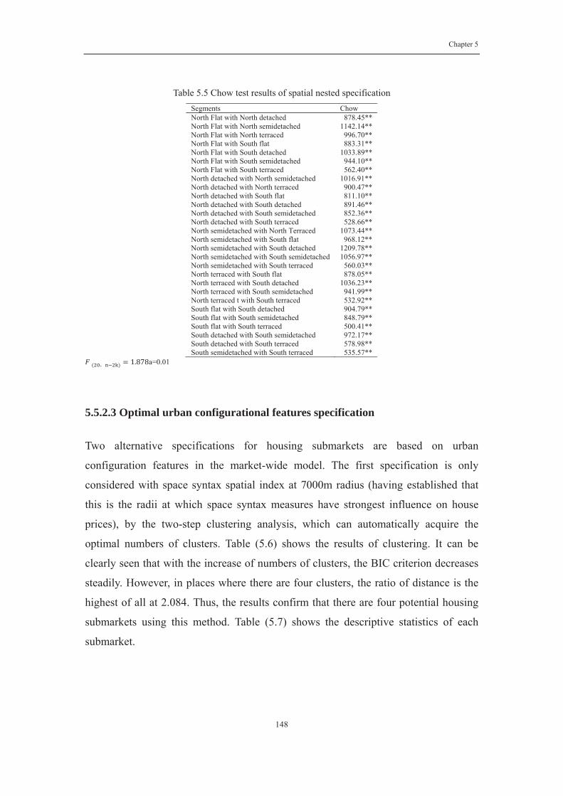
Chapter 5

148

Table 5.5 Chow test results of spatial nested specification

Segments Chow North Flat with North detached 878.45**North Flat with North semidetached 1142.14**North Flat with North terraced 996.70**North Flat with South flat 883.31**North Flat with South detached 1033.89**North Flat with South semidetached 944.10**North Flat with South terraced 562.40**North detached with North semidetached 1016.91**North detached with North terraced 900.47**North detached with South flat 811.10**North detached with South detached 891.46**North detached with South semidetached 852.36**North detached with South terraced 528.66**North semidetached with North Terraced 1073.44**North semidetached with South flat 968.12**North semidetached with South detached 1209.78**North semidetached with South semidetached 1056.97**North semidetached with South terraced 560.03**North terraced with South flat 878.05**North terraced with South detached 1036.23**North terraced with South semidetached 941.99**North terraced t with South terraced 532.92**South flat with South detached 904.79**South flat with South semidetached 848.79**South flat with South terraced 500.41**South detached with South semidetached 972.17**South detached with South terraced 578.98**South semidetached with South terraced 535.57**

a=0.01

5.5.2.3 Optimal urban configurational features specification

Two alternative specifications for housing submarkets are based on urban

configuration features in the market-wide model. The first specification is only

considered with space syntax spatial index at 7000m radius (having established that

this is the radii at which space syntax measures have strongest influence on house

prices), by the two-step clustering analysis, which can automatically acquire the

optimal numbers of clusters. Table (5.6) shows the results of clustering. It can be

clearly seen that with the increase of numbers of clusters, the BIC criterion decreases

steadily. However, in places where there are four clusters, the ratio of distance is the

highest of all at 2.084. Thus, the results confirm that there are four potential housing

submarkets using this method. Table (5.7) shows the descriptive statistics of each

submarket.

Chapter 5

149

Auto-Clustering Number of Clusters Schwarz's Bayesian

Criterion (BIC) BIC Changea Ratio of BIC

Changesb Ratio of Distance

Measuresc 1 23891.979 2 13049.078 -10842.901 1.000 1.793 3 8064.271 -4984.807 0.460 1.153 4 6297.923 -1766.349 0.163 2.084 5 4583.364 -1714.558 0.158 1.006 6 4620.152 36.788 -0.003 1.365 7 4497.368 -122.784 0.011 1.215 8 4127.028 -370.340 0.034 1.008 9 3846.759 -280.269 0.026 1.025 10 3871.099 24.340 -0.002 1.182 11 3480.348 -390.751 0.036 1.146 12 2623.182 -857.166 0.079 1.001 13 2613.258 -9.924 0.001 1.211 14 2632.163 18.905 -0.002 1.015 15 2644.196 12.033 -0.001 1.177 a. The changes are from the previous number of clusters in the table. b. The ratios of changes are relative to the change for the two cluster solution. c. The ratios of distance measures are based on the current number of clusters against the previous number of clusters.

Source: author

Figure (5.2) shows the pattern of different of urban configurational features that are

!

!

!

!

!!

!!

!

!

!

!

!

!

!

!

!

!!!!!!

!

!

!

!

!

!

!

!

!

!

!

!!!!!!!

!

!

!

!

!

!

!

!!

!

!

!!

!!!

!

!!

!

!

!

!!

!!

!

!

!

!

!

!

!

!!

!

!!!

!

!

!

!

!

!

!

!

!

!

!

!!

!

!

!

!

!!

!!

!

!

!!!

!

!

!!

!

!

!!!

!

!

!

!

!

!

!

!

!

!

!

!!

!

!

!!

!!

!

!

!

!

!

!

!!!

!! !!!

!

!

!! !!

!!

!

!!

!

!!

!

!!

!

!!

!!

!

!!

!!

!

!

!

!!

!!

!

!

!

! !!

!

!!!! !!

!!!

!

!

!

!

!

!!

!

!

!!

!

!!

!

!!

!

!

!!

!!

!

!

!!

!

!

!

!!

!

!

!!

!

!

!

!

!

!

!

!!

!

!

!

!

!

!

!

!!

!!

!

!

!

! !!

!

! ! !

!

!!!

!

!!

!!

! !

!

!

!!

!

!!

!

!

!

!

!

!

!

!

!

!

!

!

!!

!

!

!

!

!

!

!

!!!

!

!

!

!

!!!

! !!

!! !

!

!!

!

!

!

!

!

!

!!

!

!

!!

!! !

!

!

!

!

!!

!

!

!!

!

!

!!

!

!

!!

!!

!

!!!

!! !

!

!

!

!!

!!!

!

!

!!

! !

!

!

!

!

!

!

! ! !

!! !

!

!!

!!

!

!!

!

!

!!!

!

!

!!

!

!

!

!

!!!

!

!

!!

!

!! ! !

!

!

!

!

!!

!!!

!

!

!

!

!!

! !

!

!!

!

!!

! !!

!

!

!!!!!

!!

! !

!!

!!!!

! !

!!

!

!

!

!

!

!!

!!

!

!!

!

!

!

!!

!

!!

!!

!

!

! !

!!

!!

!

!

!

!!

!

!

!

!

!

!

!

!!!

!!!

!

!

!

!!

!!

!!!

!

!!

!

!

!!

!

!

!

!

!

!

!

!

!

!

!

!

!

!!!!

!!

!!

!!

!

!

!

!!

!

!

!

!

!

!!

!

!

!!

!

!

!!

!

!

!

!!

!

!

!

!

!

!

!

!

!

!

!

!!

!!

!

! !

!

!

!!

!

!

!

!

!

!

!

!

!

!

!!

!

!!

!

!!!

!

!

!

!!

!!

!!

!

!!

!

!

!

!

!!

!

!!

!

!

!!

!

! !

!!!!

!

!

!

!

! !

! !

!

!

!

!

! !

!!

!!!

!

!

!

!

!

!!

!!

!!!

!

!!

!

! !

!

!!!

!

! !

!!!

!

!

!

!

!

!

!!

!

!!!

!!

!

!!!

!!!

!!!

!

!

!

!!!!!!

!! ! !

!!!

! !

!!

!

!!!

!

!

!

!

!

!

! !

!

!!

!

!!

!

!

! !

!!

!!

!

!!

!!

!

!!

!

!!

!!

!

!!

!

!!

!

!

!

!!

!

! !!!!

!

!

!

!!

!

!

!!

!

!

!

!

!

!

!!!

!

!!

!

!

!

!

!!

!!

!

!

!!

!

!!

!

!

!

!

!

!

!

!

!

!

!

!

! !!

!

!

!

!!

!

!

!

!

!

!

!

!

!

!

!

!

!!!

!

!

!

!

!

!

!!

!!

! !

! !

!

!

!

!

!!

!

!

!! !

!! !

!!!

!!

!

!

!

!

!

! !!

!

!

!!

!

!!

!

!

!

!

!

!

!

!

!

!

!!

!

!!

!

! !

!!

!

!

!

!

!

!!

!!

!

!

!!

!!

!!!

!!

!

!

!

!!!!!

!!! !

!! !

!!!

!!!

!

!

!

!!

!!

!

!

!!

!!

!!

!!!

!

!

!!

!

!

!

!

!

!

!

!

!

!

!

!!!

!!

!

!!!

!! !

!!!!

!!

! !!!!

!

!!

!

!

!

!

!

!!!!

!

!

!

!

!!!

!

!

!

!

! !

!

!

!

!

!

!

!

!!

!

!

!!!

!

!

!!

!

!

!!

!

!

!!

!

!

!!

!

!!!

!

!

!

!

!

!

!

!

!

!

!

!

!

!

!

!

!!

!

!

!

!

!

!!

!!

!

!!

!!!

!

!!

!!!!

! !

!

!!

!!

!

!!

!

!

!

!

!!

!!!

!

!!

!

!

!

!!

!

!

!

!

!

!

! !!

!

!

!

!!

!!

!

!!

!! !!!

!

!

!

!

!

!!

!

!!

!!

!

!!

!

!

!

!

!

!

! !!

!!

!!

!

!

!

!

!

! !!!

!

!

!

!

!

!

!

!

!

!

!

!

!

!

!

!

!

!

!!

!

!!!

!

!!! !

!

!!

!

!!

!

!

!

!

!

!!!!

!

!

!

!

!!

!

!!

!!

!

!

!

!!!!!!

!!

!

!!

!

!

!

!!!

!

!!

!

!

!

!

!!!

!

!

!

!

! !!

!

!

!

!

!

!

!

!

!

!

!!

!!

!

! !

!

!

!!

!

!

!

!

!!

!

!

!

!

!

!!

!!

! !!! ! !!

!

!!

!

!

!

! !!

!

!

!

!

!

!!

! !

!

!

!

!

!

!

!

!

!

!!

!

!

!

!

!

!

!

!

!

!!

!

!! !

!!!

!!!

!

!

!

!!!

!

!

!

!!

!

!

!

!

!!

!

!

!

!

!!

!

!!

!!

!

!!

!

!

!!

!

!

! !

!

!!

!

!

!

!

!

!!

!

!

!!

!

!

!

!

!

!

!

!

!

!

!

!

!

!

!

!

!

!

!

!

!

!

!

!

!

!

!

!

!

!

!

!

!!!!

!!!!!!!!!!!!!!!!!!!!!

!

!!

!!!

!!

!

!

!!

!!

!

!

!

!!

!!

!

!

!

!

!

!

! !

!

!

!

!

!

!

!

!!

!!

!!

!

!

!

!

!

!!!

!

!!! !!

!

!!

!

!

!!

!!

!!

!!

!!

!

!!

!

!

!

!

!!

!

!

!!

!

!

!!!

!

!!!

!!

!

!!!

!! !!

!

!

!

!!

!

!

!

!

! !!

!!

!!

!!!!

!

!

!

!!

!

!

!

!!!!!

!!

!

!!

!! !!

!

!

!!

!

! !

!

!

!!!

!!

!

!

!

!!!

!

!!

!

!

!

!

!!

!!!!!

!

!

!

!!

!!!

!

!

!!

! !!

!

!

!!

!!!

!

!

!

!

!

!

! !!

!

!

!

!

!

!

!!

! !!!

!

!!!

!!

!

!!

!

!!

!

!!

!

!

!

!

!

!

!

!

!

!

!

!!!

!

! !

!

!!!

!!

!

!!

!!

!!!!

!!

!

!!!

!!!

!

!

!

!!

!!

!!

!

!!

!

!!!

!

!

!

!

!

!!

!

!! ! !

!!

!!

!!

!!!!!

! !!!

! !

!!

!!

!

!

!!! !

!

!

! !!

!

!

!

!

!!

!

!

!

!

!

!

!

!!

!

!

!!

!

!

!

!

!

! ! !

!

!

!!!

!!

!

!

!

!

!!

! !!

!

!!

!

!

!

!

!

!

!

!!!!

!!

!

!

!

!

!!

!

!

!!

!

!!

!!

!!

!

! !

!

!

!

!

!

!!

!

!

!

!!

!

!

!

!

!

!

!

!

!

!

!

!

!!

!

!

!

!

!!!

!

!

!

!!

!

!

!!!

!

!!

!

!

!

!

!!!

!!

!

!

!!

!

!

!

!!

!

!

!

!

!

!

!

!

!

!

!

!

!

!!!!

!

! !!

!

!

!

!

!

!

!

! !

!

!!!

!!

!

!

!

!

!

!

!

!

!

!

!

!

!

!!

!

!

!

!!!!

!

!

!

!

!

!!!!!!!!!!!!!!!!!!!!!!!!!!!!!!!!!!!!!!!!!!!!!!!

¯

0 910 1,820455 Meters

Two-step cluster result urban configuration features at 7000M

!

!

!

!

Cluster at radius 7000M

Chapter 5

150

associated with different spatial properties. It can be seen that submarket number one

has the highest value of both integration and choice, which might indicate that the

properties tend to be situated alongside the main streets, whilst submarket number

three has the lowest value of both integration and choice, which indicates that the

properties are located close to the boundaries of the study area. The properties of

submarket number four are mainly located at the city center but with dead-end roads,

which is why its integration is still high but the choice is low. Finally, the remaining

properties are in submarket number two, where integration is second lowest and

choice is second highest. In addition, there seems to be a clear boundary between two

parts, which indicates that the structure of spatial accessibility of urban configuration

is close to Hoyt's sector model(1939) rather than linearly diffusion concentric zone

model.

In addition, further examination of each submarket reveals that there are specific

trends of personal preference for urban configuration in the different markets. For

example, it is found that submarket one has the largest observations of all and

comprises 53.589% of all houses in the area where above 50% of properties are

terrace houses. Furthermore, in submarket one, the average housing price and floor

area are highest of all. In terms of social economic status, in submarket one, most

people are living in the city and other typical characteristics. In contrast, there are just

11.95% of total observations in submarket three, which has the cheapest average

housing price and smallest average floor area. The proportions of different social

economic status groups in submarket two and three are similar, as around one third of

people are from the blue collar group and less people are from ‘living in the city’

group, which also confirms that the demand for integration is more associated with

social economic status. As expected submarket four contains properties on the central

streets but not on the high street, which has the second largest average housing price

and third lowest floor areas. It is noted that the largest portions of social classes found

in submarket four are from city living and multiple culture groups. With regards to the

distribution of dwelling types, most detached and semidetached house are found in

submarkets two and three, which both have lower value in terms of space syntax

integration, which in turn can also indicate that the further away from the city the

bigger the size of the house. Alternatively, as I have noted already, it may be that more

Chapter 5

151

wealthy people living in large suburban houses with good car-born mobility have less

of a demand for high street network connectivity.

Cha

pter

5

152

Tabl

e 5.

7 D

escr

iptiv

e of

four

subm

arke

ts

Su

bmar

ket 1

Su

bmar

ket2

Su

bmar

ket3

Su

bmar

ket 4

N

92

21.0

00

3720

.000

20

56.0

00

2210

.000

% o

f Tot

al

53.5

89

21.6

19

11.9

49

12.8

44

N

Pe

rcen

t M

ean

N

Perc

ent

Mea

n N

Pe

rcen

t M

ean

N

Perc

ent

Mea

n

PRIC

E 92

21

100.

00%

15

1583

.201

37

20

100.

00%

1185

14.5

86

2056

10

0.00

%11

0376

.776

22

10

100.

00%

1435

47.6

79

FLO

OR

_AR

EA92

21

100.

00%

84

0.88

0 37

20

100.

00%

180.

929

2056

10

0.00

%12

0.20

2 22

10

100.

00%

121.

678

DU

_TE

7055

76

.51%

0.

765

2899

77

.93%

0.77

9 15

99

77.7

7%0.

778

1955

88

.46%

0.88

5

DU

_N

779

8.

45%

0.

084

278

7.47

%0.

075

225

10.9

4%0.

109

63

2.85

%0.

029

CH

_R70

00M

92

21

100.

00%

5.

020

3720

10

0.00

%4.

582

2056

10

0.00

%0.

034

2210

10

0.00

%0.

267

INT_

R70

00M

92

21

100.

00%

13

27.6

27

3720

10

0.00

%81

4.32

1 20

56

100.

00%

661.

191

2210

10

0.00

%11

50.7

78

DU

_D

692

7.

50%

0.

075

544

14.6

2%0.

146

314

15.2

7%0.

153

165

7.47

%0.

075

DU

_SE

1271

13

.78%

0.

138

1248

33

.55%

0.33

5 59

3 28

.84%

0.28

8 48

6 21

.99%

0.22

0

DU

_T

5308

57

.56%

0.

576

1433

38

.52%

0.38

5 86

3 41

.97%

0.42

0 13

70

61.9

9%0.

620

DU

_F

1950

21

.15%

0.

211

495

13.3

1%0.

133

286

13.9

1%0.

139

189

8.55

%0.

086

DU

_BC

16

4

1.78

%

0.01

8 96

2 25

.86%

0.25

9 63

8 31

.03%

0.31

0 95

4.

30%

0.04

3 D

U_C

L 38

41

41.6

5%

0.41

7 33

6 9.

03%

0.09

0 44

2.

14%

0.02

1 49

2 22

.26%

0.22

3

DU

_PS

1018

11

.04%

0.

110

750

20.1

6%0.

202

437

21.2

5%0.

213

327

14.8

0%0.

148

DU

_CC

10

7

1.16

%

0.01

2 36

5 9.

81%

0.09

8 22

6 10

.99%

0.11

0 84

3.

80%

0.03

8

DU

_TT

2581

27

.99%

0.

280

983

26.4

2%0.

264

612

29.7

7%0.

298

628

28.4

2%0.

284

DU

_MU

15

10

16.3

8%

0.16

4 32

4 8.

71%

0.08

7 99

4.

82%

0.04

8 58

4 26

.43%

0.26

4

Y20

00

955

10

.36%

0.

104

427

11.4

8%0.

115

207

10.0

7%0.

101

253

11.4

5%0.

114

Y20

01

1273

13

.81%

0.

139

478

12.8

5%0.

128

228

11.0

9%0.

111

308

13.9

4%0.

139

Y20

02

1437

15

.58%

0.

156

518

13.9

2%0.

139

315

15.3

2%0.

153

342

15.4

8%0.

155

Y20

03

1176

12

.75%

0.

128

518

13.9

2%0.

139

291

14.1

5%0.

142

288

13.0

3%0.

130

Y20

04

1108

12

.02%

0.

120

510

13.7

1%0.

137

316

15.3

7%0.

154

239

10.8

1%0.

108

Y20

05

912

9.

89%

0.

099

373

10.0

3%0.

100

233

11.3

3%0.

113

213

9.64

%0.

096

Y20

06

1176

12

.75%

0.

128

453

12.1

8%0.

122

219

10.6

5%0.

107

264

11.9

5%0.

119

Y20

07

1090

11

.82%

0.

118

410

11.0

2%0.

110

222

10.8

0%0.

108

279

12.6

2%0.

126

Y20

08

89

0.97

%

0.01

0 33

0.

89%

0.00

9 25

1.

22%

0.01

2 24

1.

09%

0.01

1

Chapter 5

153

Table (5.8) shows the results of four submarkets estimations specified by different

combination of high and low value of integration and choice at 7km radii. The reason

for doing this is insight how different social class are associated with different levels

of spatial accessibility.

Key findings are highlighted in the following. Firstly, the model for each submarket is

significant, and the fitness for each model seems improved, as the adjusted R-square

ranges from 0.586 to 0.719.Secondly, distance to CBD is also significant in all

submarkets, but only with a positive sign in the submarket with the highest value of

both integration, and choice. This might indicate that if the street layout is well

designed in terms of accessibility, transportation cost could be ignored. Thirdly, with

regards to configurational features, integration at radii 7km is always significant with

a positive sign in all submarkets. In the submarket which has high integration and the

lowest choice, it is found that choice is insignificant because the properties of this

submarket are alongside the main street or near the city center but with dead-end

street segments. Moreover, choice is found to be significant but with a positive sign in

the submarket which is lowest both in terms of integration and choice. Properties in

this submarket are communities in suburb urban areas; the high choice value has a

positive impact and the reason maybe because it is associated with low crime rate.

Fourthly, since the people of “constrained by circumstances” have a small portion in

submarket two and three, where the street segments are less connected, it is expected

to be insignificant. Moreover, all classes are significant in all submarket at 5%

confidence level, which provides the evidence that social economic status can also

impact on the submarket specified by urban configuration features. Finally, the results

of Chow tests are shown in table (5.9). All six F-statistics are significant at the 0.1

level and the null hypotheses are rejected with a high level of confidence, confirming

the existence of four submarkets.

Chapter 5

154

Submarket 1 Submarket 2 Submarket3 Submarket 4

N 9221 3720 2056 2210

Adjust R-square

0.586 0.711 0.719 0.643

F test 601.324 396.022 221.740 189.305

RSS 1180.303 299.322 122.851 239.118

t Sig. t Sig. t Sig. t Sig.

(Constant) -5.888 0.000** 2.628 0.009** 11.053 0.000** 6.312 0.000**

LN_FL 30.935 0.000** 2.713 0.007** 6.230 0.000** 11.817 0.000**

LN_D 6.152 0.000** -2.324 0.020* -10.830 0.000** -6.157 0.000**

DU_N 7.074 0.000** 11.791 0.000** 4.260 0.000** 7.047 0.000**

DU_D 25.115 0.000** 27.623 0.000** 21.898 0.000** 6.996 0.000**

DU_SE 16.377 0.000** 17.015 0.000** 15.385 0.000** 3.922 0.000**

DU_T 9.051 0.000** 8.906 0.000** 9.625 0.000** 0.050 0.960

DU_TE 17.499 0.000** 2.404 0.016* -0.532 0.595 10.065 0.000**

DU_CL 14.986 0.000** 3.887 0.000** 6.586 0.000** 8.477 0.000**

DU_PS 24.783 0.000** 24.836 0.000** 16.522 0.000** 20.797 0.000**

DU_CC 3.495 0.000** 0.893* 0.372** 0.015* 0.988 5.650 0.000**

DU_TT 11.279 0.000** 12.049 0.000** 7.974 0.000** 15.437 0.000**

Y2001 6.740 0.000** 6.571 0.000** 1.582 0.114 4.830 0.000**

Y2002 19.073 0.000** 14.131 0.000** 8.776 0.000** 10.474 0.000**

Y2003 29.827 0.000** 25.560 0.000** 18.844 0.000** 19.050 0.000**

Y2004 40.701 0.000** 34.363 0.000** 25.168 0.000** 21.586 0.000**

Y2005 43.779 0.000** 37.298 0.000** 29.104 0.000** 24.638 0.000**

Y2006 48.185 0.000** 40.963 0.000** 30.417 0.000** 27.323 0.000**

Y2007 49.768 0.000** 42.097 0.000** 32.201 0.000** 29.498 0.000**

Y2008 19.566 0.000** 16.108 0.000** 14.880 0.000** 10.981 0.000**

CH_R7000M -9.791 0.000** -4.311 0.000** 4.068 0.000** -0.717* 0.473

INT_R7000M 16.276 0.000** 7.041 0.000** 1.998 0.046* 8.717 0.000**

NSV 21 20 19 19

p <0.05 ** P<0.01

NSV = number of significant variable

Segments Chow 1 with 2 183.431 with 3 250.541 with 4 190.782 with 3 938.332 with 4 697.713 with 4 838.02

a=0.01

Chapter 5

155

5.5.2.4 Nested urban configuration and dwelling type specification

The second way to specify housing submarket is to nest both dwelling types and

urban configuration features at radii 7km. The reasons of justification for this

approach are two folds: firstly, compared with traditional specification only by

dwelling types, I expect considering the all urban configurational features could

improve the estimation. Furthermore, I also expect to compare the performance of

specifications by dwelling types within the pre-defined geographical area and new

alternative spatial areas. The two-step clustering analysis results are showed in table

(5.10), although the ratio of distance of both four and five clusters are higher than

others, five clusters has the smallest ratio of BIC change, thus, the optimal numbers of

submarket specified by nesting both dwelling types and urban configuration features

is five.

Figure (5.3) shows the spatial pattern of the five housing submarkets. It is found that

building structure characteristics (e.g. detached, semidetached, terrace and flat) have

the strongest influence on the five housing submarkets, and each building type is

associated with a different combinations of high and low values of integration and

choice. For example, the submarket of flats is associated with high street connections

and high traffic flow, and detached and semidetached houses require similar urban

configuration features with lowest integration and higher choice values. Furthermore,

it is noted that the largest portion of building type is terraced housing, and it is divided

into two groups which are associated with high and low space syntax integration and

choice. Two thirds of terrace houses are in cluster two and are located in places with

the highest accessibility and highest traffic volume whereas the rest of the terraced

housing are located in cluster three with street segments less connected and lower

levels of traffic volume.

By examining the social economic status of the residents in each submarket, it is

possible to state that different demands from different classes cause housing market

segmentation. For example, as expected, the largest group of people who choose flats

are from the “city living” group. More than half of the people who choose detached

housing are from the group “prospering suburbs”, and “prospering suburbs” and

Chapter 5

156

“typical traits” take up nearly two thirds of the people choosing semi-detached

housing. In comparison, the other terraced-housing submarket, which has higher

choice and integration value, is mainly occupied by the city living cohort and people

of similar socioeconomic characteristics such as blue collars group,. This in turn

implies that the location of this submarket is near the city center. With regards to

terrace houses that have different configurational features, the proportion of different

socio-economic classes are slightly different. For example, it is found that more

people from the “blue collar” group and less “city living” prefer terraced housing

located in urban suburb areas, which have lower street segment connectivity and

traffic flow.

Table 5.10 Cluster results of nested urban configuration and building type specification

Auto-Clustering Number of Clusters Schwarz's Bayesian

Criterion (BIC) BIC Changea Ratio of BIC

Changesb Ratio of Distance

Measuresc 1 92234.001 2 54172.863 -38061.138 1.000 2.063 3 35766.199 -18406.664 0.484 1.477 4 23328.847 -12437.352 0.327 2.319 5 18010.103 -5318.744 0.140 2.268 6 15708.879 -2301.224 0.060 1.017 7 13448.247 -2260.632 0.059 1.312 8 11743.573 -1704.674 0.045 1.429 9 10573.904 -1169.670 0.031 1.216 10 9625.946 -947.958 0.025 1.006 11 8683.699 -942.247 0.025 1.058 12 7797.218 -886.480 0.023 1.484 13 7225.345 -571.874 0.015 1.309 14 6806.877 -418.467 0.011 1.132 15 6446.276 -360.602 0.009 1.149 a. The changes are from the previous number of clusters in the table. b. The ratios of changes are relative to the change for the two cluster solution. c. The ratios of distance measures are based on the current number of clusters against the previous number of clusters.

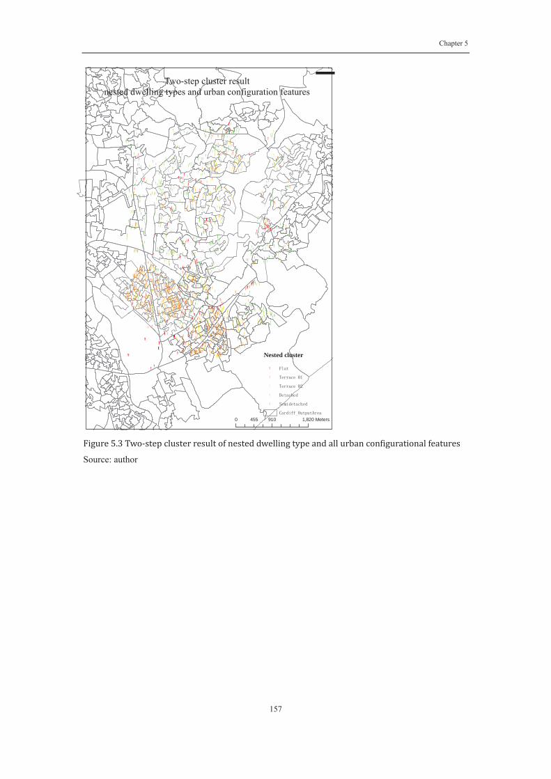
Chapter 5

157

Source: author

!

!

!

!

!!

!!

!

!

!

!

!

!

!

!

!

!!!!!!

!

!

!

!

!

!

!

!

!

!

!

!!!!!!!

!

!

!

!

!

!

!

!!

!

!

!!

!!!

!

!

!

!

!

!

!!

!!

!

!

!

!

!

!

!

!!

!

!!!

!

!

!

!

!

!

!

!

!

!

!

!!

!

!

!

!

!!

!!

!

!

!!!

!

!

!!

!

!

!!!

!

!

!

!

!

!

!

!

!

!

!

!!

!

!

!!

!!

!

!

!

!

!

!

!!!

!! !!!

!

!

!! !!

!!

!

!!

!

!!

!

!!

!

!!

!!

!

!!

!!

!

!

!

!!

!!

!

!

!

! !!

!

!!!! !!

!!!

!

!

!

!

!

!!

!

!

!!

!

!!

!

!!

!

!

!!

!!

!

!

!!

!

!

!

!!

!

!

!!

!

!

!

!

!

!

!

!!

!

!

!

!

!

!

!

!!

!!

!

!

!

! !!

!

! ! !

!

!

!!

!

!!

!!

! !

!

!

!!

!

!!

!

!

!

!

!

!

!

!

!

!

!

!

!!

!

!

!

!

!

!

!

!!!

!

!

!

!

!!!

! !!

!! !

!

!!

!

!

!

!

!

!

!!

!

!

!!

!! !

!

!

!

!

!!

!

!

!!

!

!

!!

!

!

!!

!!

!

!!!

!! !

!

!

!

!!

!!!

!

!

!!

! !

!

!

!

!

!

!

! ! !

!! !

!

!!

!!

!

!!

!

!

!!!

!

!

!!

!

!

!

!

!!!

!

!

!!

!

!! ! !

!

!

!

!

!!

!!!

!

!

!

!

!!

! !

!

!!

!

!!

! !!

!

!

!!!!

! !!

! !

!!

!!!!

! !

!!

!

!

!

!

!

!

!

!!

!

!!

!

!

!

!!

!

!!

!!

!

!

! !

!!

!!

!

!

!

!!

!

!

!

!

!

!

!

!!!

!!!

!

!

!

!!

!!

!!!

!

!!

!

!

!!

!

!

!

!

!

!

!

!

!

!

!

!

!

!!!!

!!

!!

!!

!

!

!

!!

!

!

!

!

!

!!

!

!

!!

!

!

!!

!

!

!

!!

!

!

!

!

!

!

!

!

!

!

!

!!

!

!

!

! !

!

!

!!

!

!

!

!

!

!

!

!

!

!

!!

!

!!

!

!!!

!

!

!

!!

!!

!!

!

!!

!

!

!

!

!!

!

!!

!

!

!!

!

! !

!!!!

!

!

!

!

! !

! !

!

!

!

!

! !

!!

!!!

!

!

!

!

!

!!

!!

!!!

!

!!

!

! !

!

!!!

!

! !

!!!

!

!

!

!

!

!

!!

!

!!!

!!

!

!!

!

!!!

!!!

!

!

!

!!!!!!

!! ! !

!!!

! !

!!

!

!!!

!

!

!

!

!

!

! !

!

!!

!

!!

!

!

! !

!!

!!

!

!!

!!

!

!!

!

!!

!!

!

!!

!

!!

!

!

!

!!

!

! !!!!

!

!

!

!!

!

!

!!

!

!

!

!

!

!

!!!

!

!

!

!

!

!

!

!!

!!

!

!

!!

!

!!

!

!

!

!

!

!

!

!

!

!

!

!

! !!

!

!

!

!!

!

!

!

!

!

!

!

!

!

!

!

!

!!!

!

!

!

!

!

!

!!

!!

! !

! !

!

!

!

!

!!

!

!

!! !

!! !

!!!

!!

!

!

!

!

!

! !!

!

!

!!

!

!!

!

!

!

!

!

!

!

!

!

!

!!

!

!!

!

! !

!!

!

!

!

!

!

!!

!!

!

!

!!

!!

!!!

!!

!

!

!

!!!!!

!!! !

!! !

!!!

!!!

!

!

!

!!

!!

!

!

!!

!!

!!

!!

!

!

!

!!

!

!

!

!

!

!

!

!

!

!

!

!!!

!!

!

!!!

!! !

!!!!

!!

! !!!!

!

!!

!

!

!

!

!

!!!!

!

!

!

!

!!!

!

!

!

!

! !

!

!

!

!

!

!

!

!!

!

!

!!!

!

!

!!

!

!

!!

!

!

!

!

!

!

!!

!

!!!

!

!

!

!

!

!

!

!

!

!

!

!

!

!

!

!

!!

!

!

!

!

!

!!

!!

!

!!

!!!

!

!!

!!!!

! !

!

!!

!!

!

!!

!

!

!

!

!!

!!!

!

!!

!

!

!

!!

!

!

!

!

!

!

! !!

!

!

!

!!

!!

!

!!

!! !!!

!

!

!

!

!

!!

!

!!

!!

!

!!

!

!

!

!

!

!

! !!

!!

!!

!

!

!

!

!

! !!!

!

!

!

!

!

!

!

!

!

!

!

!

!

!

!

!

!

!

!!

!

!!!

!

!!! !

!

!!

!

!!

!

!

!

!

!

!!!!

!

!

!

!

!!

!

!!

!!

!

!

!

!!!!!!

!!

!

!!

!

!

!

!

!!

!

!!

!

!

!

!

!

!!

!

!

!

!

! !!

!

!

!

!

!

!

!

!

!

!

!!

!!

!

!!

!

!

!!

!

!

!

!

!!

!

!

!

!

!

!!

!!

! !!! ! !!

!

!!

!

!

!

! !!

!

!

!

!

!

!!

! !

!

!

!

!

!

!

!

!

!

!!

!

!

!

!

!

!

!

!

!

!!

!

!

! !!!!

!!!

!

!

!

!!!

!

!

!

!!

!

!

!

!

!!

!

!

!

!

!!

!

!!

!!

!

!!

!

!

!!

!

!

! !

!

!!

!

!

!

!

!

!!

!

!

!!

!

!

!

!

!

!

!

!

!

!

!

!

!

!

!

!

!

!

!

!

!

!

!

!

!

!

!

!

!

!

!

!

!

!!!

!!!!!!!!!!!!!!!!!!!!!

!

!

!

!!!

!!

!

!

!!

!!

!

!

!

!!

!!

!

!

!

!

!

!

! !

!

!

!

!

!

!

!

!!

!!

!!

!

!

!

!

!

!!!

!

!!! !!

!

!!

!

!

!!

!!

!!

!!

!!

!

!!

!

!

!

!

!!

!

!

!!

!

!

!!!

!

!!

!

!

!

!

!!!

!! !!

!

!

!

!!

!

!

!

!

! !!

!!

!!

!!!!

!

!

!

!!

!

!

!

!!!!!

!!

!

!!

!! !!

!

!

!!

!

! !

!

!

!!!

!!

!

!

!

!!!

!

!!

!

!

!

!

!!

!!!!!

!

!

!

!!

!!!

!

!

!!

! !!

!

!

!!

!!!

!

!

!

!

!

!

! !!

!

!

!

!

!

!

!!

! !!!

!

!!!

!!

!

!!

!

!!

!

!!

!

!

!

!

!

!

!

!

!

!

!

!!!

!

! !

!

!!!

!!

!

!!

!!

!!!!

!!

!

!!!

!!!

!

!

!

!!

!!

!!

!

!!

!

!!!

!

!

!

!

!

!!

!

!! ! !

!!

!!

!!

!!!!!

! !!!

! !

!!

!!

!

!

!!! !

!

!

! !!

!

!

!

!

!!

!

!

!

!

!

!

!

!!

!

!

!!

!

!

!

!

!

! ! !

!

!

!!!

!!

!

!

!

!

!!

! !!

!

!!

!

!

!

!

!

!

!

!!!!

!!

!

!

!

!

!!

!

!

!!

!

!!

!!

!!

!

! !

!

!

!

!

!

!!

!

!

!

!!

!

!

!

!

!

!

!

!

!

!

!

!

!!

!

!

!

!

!!!

!

!

!

!!

!

!

!!!

!

!!

!

!

!

!

!!!

!!

!

!

!!

!

!

!

!!

!

!

!

!

!

!

!

!

!

!

!

!

!

!!!!

!

! !!

!

!

!

!

!

!

!

! !

!

!!!

!!

!

!

!

!

!

!

!

!

!

!

!

!

!

!!

!

!

!

!!!!

!

!

!

!

!

!!!!!!!!!!!!!!!!!!!!!!!!!!!!!!!!!!!!!!!!!!!!!!!

¯

0 910 1,820455 Meters

Two-step cluster result nested dwelling types and urban configuration features

Nested cluster

!

!

!

!

!

Cha

pter

5

158

Su

bmar

ket 1

Su

bmar

ket 2

Su

bmar

ket 3

Su

bmar

ket 4

Su

bmar

ket 5

N

29

20

6788

21

86

1715

35

98

% o

f Tot

al

16.9

70

39.4

49

12.7

04

9.96

7

20.9

10

N

Pe

rcen

t M

ean

N

Perc

ent

Mea

n N

Pe

rcen

t M

ean

N

Perc

ent

Mea

n N

Pe

rcen

tM

ean

PRIC

E 29

20

100.

00%

11

7963

.919

67

88

100.

00%

1229

01.4

19

2186

10

0.00

%10

9085

.606

17

1510

0.00

%23

9515

.736

35

9810

0.00

%15

4212

.862

FLO

OR

_AR

EA29

20

100.

00%

25

49.2

23

6788

10

0.00

%10

6.00

1 21

86

100.

00%

90.2

99

1715

100.

00%

124.

215

3598

100.

00%

102.

604

DU

_N

856

29.3

2%

0.29

3 32

0.

47%

0.00

5 8

0.37

%0.

004

21

912

.77%

0.12

8 23

06.

39%

0.06

4

DU

_TE

62

2.12

%

0.02

1 64

52

95.0

5%0.

951

2051

93

.82%

0.93

8

1654

96.4

4%0.

964

3289

91.4

1%0.

914

CH

_R70

00M

29

20

100.

00%

4.

494

6788

10

0.00

%4.

700

2186

10

0.00

%0.

154

17

1510

0.00

%3.

602

3598

100.

00%

3.46

3

INT_

R70

00M

29

20

100.

00%

12

01.2

37

6788

10

0.00

%12

11.6

99

2186

10

0.00

%96

1.83

6

1715

100.

00%

1011

.954

35

9810

0.00

%10

01.4

61

DU

_D

0 0.

00%

0.

000

0 0.

00%

0.00

0 0

0.00

%0.

000

17

1510

0.00

%1.

000

00.

00%

0.00

0 D

U_S

E 0

0.00

%

0.00

0 0

0.00

%0.

000

0 0.

00%

0.00

0

00.

00%

0.00

0 35

9810

0.00

%1.

000

DU

_T

0 0.

00%

0.

000

6788

10

0.00

%1.

000

2186

10

0.00

%1.

000

0

0.00

%0.

000

00.

00%

0.00

0

DU

_F

2920

10

0.00

%

1.00

0 0

0.00

%0.

000

0 0.

00%

0.00

0

00.

00%

0.00

0 0

0.00

%0.

000

DU

_BC

42

1.

44%

0.

014

642

9.46

%0.

095

495

22.6

4%0.

226

67

3.91

%0.

039

613

17.0

4%0.

170

DU

_CL

1621

55

.51%

0.

555

2145

31

.60%

0.31

6 29

8 13

.63%

0.13

6

202

11.7

8%0.

118

447

12.4

2%0.

124

DU

_PS

199

6.82

%

0.06

8 12

2 1.

80%

0.01

8 75

3.

43%

0.03

4

1003

58.4

8%0.

585

1133

31.4

9%0.

315

DU

_CC

20

6 7.

05%

0.

071

207

3.05

%0.

030

121

5.54

%0.

055

34

1.98

%0.

020

214

5.95

%0.

059

DU

_TT

492

16.8

5%

0.16

8 23

59

34.7

5%0.

348

638

29.1

9%0.

292

34

520

.12%

0.20

1 97

026

.96%

0.27

0

DU

_MU

36

0 12

.33%

0.

123

1313

19

.34%

0.19

3 55

9 25

.57%

0.25

6

643.

73%

0.03

7 22

16.

14%

0.06

1

Y20

00

200

6.85

%

0.06

8 79

7 11

.74%

0.11

7 26

3 12

.03%

0.12

0

202

11.7

8%0.

118

380

10.5

6%0.

106

Y20

01

247

8.46

%

0.08

5 10

88

16.0

3%0.

160

303

13.8

6%0.

139

18

210

.61%

0.10

6 47

213

.12%

0.13

1

Y20

02

435

14.9

0%

0.14

9 10

44

15.3

8%0.

154

345

15.7

8%0.

158

29

717

.32%

0.17

3 49

113

.65%

0.13

6

Y20

03

447

15.3

1%

0.15

3 86

1 12

.68%

0.12

7 29

9 13

.68%

0.13

7

209

12.1

9%0.

122

457

12.7

0%0.

127

Y20

04

423

14.4

9%

0.14

5 75

9 11

.18%

0.11

2 23

8 10

.89%

0.10

9

225

13.1

2%0.

131

528

14.6

7%0.

147

Y20

05

368

12.6

0%

0.12

6 61

8 9.

10%

0.09

1 20

0 9.

15%

0.09

1

185

10.7

9%0.

108

360

10.0

1%0.

100

Y20

06

357

12.2

3%

0.12

2 85

5 12

.60%

0.12

6 25

2 11

.53%

0.11

5

202

11.7

8%0.

118

446

12.4

0%0.

124

Y20

07

415

14.2

1%

0.14

2 70

6 10

.40%

0.10

4 26

3 12

.03%

0.12

0

200

11.6

6%0.

117

417

11.5

9%0.

116

Y20

08

28

0.96

%

0.01

0 60

0.

88%

0.00

9 23

1.

05%

0.01

1

130.

76%

0.00

8 47

1.31

%0.

013

Chapter 5

159

Table (5.12) shows the results of five submarkets estimation specified by nested

dwelling types and all urban configuration features. Key findings are highlighted as

follows. Firstly, all models of the five submarkets have good results, since all F tests

are significant and the adjusted R-square is within the range of 0.56 to 0.65. Secondly,

the location characteristic of distance to CBD is significant with a negative sign and

found in the submarket of urban suburb area, where both “integration” and “choice”

are not high. Thirdly, the sign of urban configuration is constant, but it is found that

urban configurational features do not impact the submarket of detached houses, as

both integration and choice at 7km radii are insignificant at 5% level. Furthermore,

choice is also found insignificant in the terraced submarket in suburban areas, as the

variance of traffic flow is much lower in suburbs than centrally. This indicates that

comparing inner-city and outer-city, when people choose their properties, they do not

care about the traffic flow in the outer-city. Fourthly, it is seen that people

“constrained by circumstances” are more sensitive to the submarkets associated with

high value of choice, as the variable is insignificant in both submarket two and three.

The results of the Chow tests for structural change in pricing models are presented in

table (5.13). All F tests are significant at 0.01 level of confidence, showing that there

is strong evidence to support the existence of five submarkets using this method.

Table 5.12 Estimation results of nested all urban configurational features and building type

specification

Submarket 1 Submarket 2 Submarket 3 Submarket 4 Submarket 5

N 2920 6788 2186 1715 3598

Adjust R-square 0.638 0.565 0.628 0.591 0.654

F test 272.082 474.976 200.454 115.747 358.349

RSS 315.488 736.618 207.866 186.696 320.484

t Sig. t Sig. t Sig. t Sig. t Sig.

(Constant) 1.238 0.216 -4.338 0.000** 6.783 0.000** 2.352 0.019* 6.849 0.000**

LN_FL 14.430 0.000** 22.954 0.000** 8.843 0.000** 23.663 0.000** 21.904 0.000**

LN_D -1.046* 0.296 4.600 0.000** -6.577 0.000** -2.248 0.025* -6.590 0.000**

DU_N 15.455 0.000** 2.348 0.019* 1.235* 0.217 2.126 0.034* 9.951 0.000**

DU_TE 5.171 0.000** 13.480 0.000** 3.841 0.000** 13.389 0.000** 8.304 0.000**

Chapter 5

160

DU_CL 6.629 0.000** 11.257 0.000** 4.844 0.000** 5.479 0.000** 8.639 0.000**

DU_PS 19.342 0.000** 9.145 0.000** 8.521 0.000** 15.323 0.000** 26.534 0.000**

DU_CC 1.177 0.239 3.051 0.002** 1.111 0.267 2.281 0.023* 3.560 0.000**

DU_TT 5.558 0.000** 9.694 0.000** 14.916 0.000** 6.028 0.000** 13.156 0.000**

Y2001 4.226 0.000** 7.543 0.000** 3.848 0.000** 3.140 0.002** 5.067 0.000**

Y2002 11.886 0.000** 19.474 0.000** 9.382 0.000** 5.949 0.000** 13.545 0.000**

Y2003 16.896 0.000** 33.003 0.000** 20.076 0.000** 10.066 0.000** 22.406 0.000**

Y2004 23.565 0.000** 41.305 0.000** 25.291 0.000** 13.389 0.000** 29.451 0.000**

Y2005 27.309 0.000** 43.285 0.000** 26.776 0.000** 16.823 0.000** 31.807 0.000**

Y2006 28.280 0.000** 48.603 0.000** 30.735 0.000** 17.075 0.000** 34.536 0.000**

Y2007 29.400 0.000** 49.810 0.000** 32.361 0.000** 19.014 0.000** 35.497 0.000**

Y2008 11.116 0.000** 19.396 0.000** 14.398 0.000** 6.418 0.000** 15.606 0.000**

CH_R7000M -7.366 0.000** -9.057 0.000** -1.329 0.184 1.532 0.126 -3.174 0.002**

INT_R7000M 11.917 0.000** 19.618 0.000** 6.499 0.000** 1.594 0.111 9.957 0.000**

NSV 16 18 15 16

p <0.05 ** P<0.01

NSV = number of significant variable

Table 5.13 Chow test results of nested all urban configurational features and building type specification

Segments Chow

Submarket 1 with 2 420.83**

Submarket 1 with3 715.49**









a=0.01

5.5.3 Estimation of weighed standard error

Chapter 5

161

Stratification scheme Standard error % reduction

Market-wide model 1942.597

Structure definition identified by dwelling type 642.615 66.92%

Nested definition identified by dwelling-type segments in north and south 394.090 79.71%

Submarket specified only by urban configuration at 7000M radius 744.060 61.70%

Submarket specified by both urban configuration and dwelling types at 7000M radii 456.726 76.49%

Finally, i use the weighted standard test applied by Schnare and Struyk(1976) to

evaluate the improvement of segmented market models in terms of standard error

estimation. For the weighted standard error test, there is no strict requirement on the

size of the low threshold of evidence, or significance and overall variability in

housing prices. Schnare and Struyk accepted this threshold as 10 percent in their

studies whereas Dale and Johnson (1982) suggested five percent. The two new

alternative methods and the two traditional methods defining the housing submarket

all pass the weighted standard error test, even at the strictest level, as shown in table

(5.14).

From that table (5.14), it is possible to see that the method specifying submarkets

using nested spatial indicator and structure with prior experience has the best results,

which has improved the market-wide estimation by 79.71%. The second best

performance specification is defining submarkets by both urban configuration and

dwelling types at 7000m radii, which has improved the error rate by 76.49%. The

third best is the structure definition by dwelling type.

Although the new method identifying submarkets only by urban configuration

features at radii 7km, is not the best, the model has still improved the estimation by

61.70%. The spatial and structure nested method has the best performance overall

since it is an ad hoc method. The urban configuration and dwelling types nested

identification is slightly weaker than the traditional spatial and structure nested model,

but the whole process can be deemed more objective. As Orford (2000) highlighted,

Chapter 5

162

the building structure features are important for housing submarkets in Cardiff

housing market, which means that the housing market in Cardiff can be segmented

according to its building structure features. In this case, each building type group

reflects the price unit of each characteristic and people’s willingness to pay is constant.

However, the results of clustering nested building types and urban configurational

features shows that each building type is associated with specific combination of high

and low integration and choice values, which suggests that the building structure

features interact with urban configurational features in complex ways. Furthermore,

the weighed standard error test shows the improvements of specification by building

type and the optimal urban configurational features are quite close with a difference of

only 5.22%.

On the basis of these results, it may be suggested that for housing markets where the

dwelling type is uniform, urban configurational features could be an alternative

specification method for submarkets, since I have shown that there is heterogeneous

demand within the housing market as a whole for different kinds and levels of

network connectivity and conversely, and different classes of people have

homogeneous demand for urban configurational features of housing property. Cardiff

proves to be an interesting location for this experiment since it has become obvious

that the strong distinctions made in the market between building-types, means that

this becomes a dominant dimension in creating sub-markets. In spite of this, network

configuration measured by space syntax still adds discriminating power in explaining

differences in clusters of house prices. I can be sure therefore that in markets with far

more homogenous housing stock such as Chinese cities, urban configuration is likely

to be an important determinant in sub-market formation.

5.6 Summary

This study supports the large amount of researches into the means of identifying

Chapter 5

163

housing submarkets that have found that building structure features are important

inreflecting people’s homogenous perceptions towards property attributes. However,

it has added new knowledge designed to address the lack of understanding about how

to deal with submarkets when the dwelling type is homogenous, for example

uniformly simplex as in many Chinese cities. I have shown that configurational data

recovered from a graph model of a street network adds significant power in

discriminating between housing sub-markets and thus provides a potentially fruitful

approach to analyzing sub-markets in China.

Although a non-spatial specification of sub-markets can to a degree relieve some of

the problems of traditional ad hoc geographical sub-market specification these

methods require social neighborhood characteristics to be constant over time and such

methods are thus ill-fitted to rapidly transforming countries. The objective of this

study has therefore been to test whether urban configurational features can offer a new

alternative way to specify housing submarkets, since network configuration is likely

to be more stable than other neighborhood characteristics. The accessibility metrics

derived from space syntax models of housing areas would intuitively seem to be

important contributors to locational value. In order to verify the assertion, I have

compared the model performances of network-based sub-market specifications

against traditional means. Two alternative methods were specified: one used only

optimally measured urban configurational features, and the other used nested optimal

urban configurational feature combined with dwelling types.

Two-step clustering analysis found that both building types and social economic

classes are associated with the indicators of space syntax namely integration and

choice. For example, flats require street segments with high levels of street

connectivity and high traffic flow whereas detached and semidetached houses require

similar urban configuration where street connection is poor but with high levels of

traffic flow. Furthermore, people of middle class cohorts or above tend to live further

Chapter 5

164

away from the city center since they have access to cars and consequently are less

sensitive to how well street segments are connected. This is in stark contrast to lower

income people who are sensitive to the geometrical pattern of street segments.

Finally, the weighted standard error tests show that all specifications using space

syntax metrics have significantly improved the estimation over and above the

market-wide model. Although the specifications based on urban configurational

features are not the best performing models, these results are quite close to the

traditional specifications and they are (a) more objective in their approach and (b) less

reliant on a housing market culture that has evolved around distinctly differentiated

building types. Therefore, it seems justifiable to conclude that a housing sub-market

model based on urban configurational features can be an alternative way to deal with

cases where the building type is uniformly simplex and where there are low levels of

observations of social neighborhood preferences.

Chapter 6

165

Chapter Six:

Identifying the micro-dynamic effects of urban street configuration on house price volatility using a panel model

For the majority of households, housing represents the main component of wealth,

and the “wealth effect” of housing on consumption is significant (Case et al. 2005).

Furthermore, the housing market impacts the economy not only through wealth

effects, but also has influences on other markets (e.g. the mortgage market, mortgage

insurance, mortgage backed bonds, and consumer durables). Therefore, understanding

the sources of housing market price volatility has great significance or the wider

economy and the welfare of society. Despite the importance of the housing market,

most empirical analyses mainly focus on exploring the macro determinants of house

price movements over time using aggregated data (e.g. real income, real GDP, tax

rates, interest rates, population, construction costs and consumer price index) (Holly

and Jones 1997; Hort 1998; Takala and Barot 1998; Meese and Wallace 2003;

Harter-Dreiman 2004; Riddel 2004). At the micro level, there are also researchers

who identify the price impact of one-time changes of building characteristic,

measuring the added value for housing price over time by hybrid repeat sales models

and hedonic models (McMillen 2003; Case et al. 2006; McMillen and Thorsnes 2006;

Tian 2006; Noonan 2007). However, hybrid repeat sales and hedonic models have

been criticized for the basis of sample selection and underestimation (Polinsky and

Rubinfeld 1977; Polinsky and Shavell 1982). Recently, Iacono and Levinson (2011)

examined the micro dynamic relationship between accessibility and land value over

Chapter 6

166

time by first difference estimation. They used property sales data of Minneapolis-St.

Paul region for the years 2000 and 2005, and measured of accessibility combined with

regional accessibility data for their respective years to predict changes in prices over

time in a particular location. However, they failed to find any significant micro

dynamic effects of accessibility on land value over time. They also noted that

measuring changes in accessibility should be described more accurately than they

were able to. Although these approaches could address the problem of omitted

variable, they do not consider the unobserved heterogeneity variation over time (e.g.

housing policy change and construction cost change), and assume the macro factors to

be constant, which also may lead to estimation bias.

However, few studies have examined geographical determinants of house price

volatility within a region or city scale, although many scholars assert that the value of

accessibility could lead to changes in housing price dynamics (Capozza and Helsley

1989). Currently, China is undergoing rapid the urbanization, and with respect to its

scale, it is perhaps the largest the world has ever experienced (Zhang and Song 2003).

As part of this process, there have been numerous investments into road network

developments situated on the urban fringe in order to cope with the rapid expansion of

cities and its populations (Zhang and Zhao 2009). In most Chinese cities, it is easy to

observe how rapid urban spatial expansion can impact on the dynamic change of

housing price in the local housing market, especially after 2003. Many house

purchasers found that the price of properties located near existing or future transport

hubs are more likely to increase. Consequently, housing buyers tend to have a clear

belief that infrastructure improvement projects will add further value to their property.

Against this background, the study readdresses the hypothesis that there is a

micro-dynamic relationship between urban morphology and housing price, using a

large panel dataset for city of Nanjing, China from 2005 to 2010.Three main

questions are answered in this study. Firstly, is there a micro-dynamic relationship

Chapter 6

167

between urban morphology and housing price? Secondly, do all street network

improvements produce a positive spillover effect captured in property value; and if

not then what kind of street network improvement and at what scale are such

improvements good for the house owner? Thirdly, I ask whether this relationship is

dynamic synchronously over both space and time, and whether submarkets exist as a

result of accessibility patterns.

Compared with previous studies, several points should be made. Firstly, the study

applies the average selling price rather than the transaction price from survey data.

The reasons for this are explained at a later point of this chapter. Secondly, a

location-based social network analysis method, known as space syntax, is employed

in this study to capture the accessibility changes created by street network

improvements over time. Thirdly, I ran a random intercept model instead of

alternatives such as a first difference model, hybrid repeat sale model and hedonic

model, as during the period in which the data was gathered, housing policy governing

the regulation of multiple properties changed several times, thus the unobserved

heterogeneity could be absorbed by the intercept in a fixed effect model. Furthermore,

the assumptions of a first difference model are less restrictive than the assumptions of

weak exogeneity required for an unbiased fixed effects (FE) estimator (i.e.

homoscedasticity and no serial correlation in error term). A fixed effects model is

efficient under independence of error term and a first difference model is efficient

under perfect serial correlation in the error term (Mendelsohn et al. 1992).

The structure of this chapter is organized as follows: in section two, I review studies

that examine housing price volatility both at macro and micro level. In section three,

space syntax network analysis and longitudinal random intercept models are

explained and illustrated. Section four introduces the study area and survey data, and

results are presented in Section five, utilizing five different models (e.g. pooled model,

individual-fixed effects model, random effects model, time-fixed effect model and

Chapter 6

168

two-way effects model). Insights from the empirical results are discussed in section 6;

and Section 7 summarizes the findings and concludes.

6.2.1 Cross-sectional static house price models

Urban researchers have long recognized the limitations of the monocentric concept on

several levels (e.g. polycentric employment, assumption of exogenous employment

location) (e.g. Boarnet 1994). As an alternative, the notion of accessibility is taken by

most researchers exploring the locational determinants of house price following

Rosen’s (1974b) hedonic price model based on cross-section data. Some researchers

have found that accessibility in terms of easy access to different services (such as rail

station) adds value to properties. For example, Dewees (1976) explored the rail travel

costs’ impact on residential property values, and he found that a subway station

increases the site rent with a radii of one third mile. In a similar study, Bowes and

Ihlanfeldt (2001) found that rail stations with parking facilities have a higher positive

impact on housing price, but its impact power still depends on how proximity to the

CBD. In fact, the most megacity shows a tendency of ploycentric in spatial, such as

Osland and Thorsen (2008)explored the effect of urban attraction and labor-market

accessibility on housing price by utilizing a gravity-based labor-market accessibility.

They found that labor-market accessibility is not an adequate alternative to distance

from the CBD; illustrating that there are multiple attributes bundled into the concepts

of central accessibility. Recently, Adair et al. (2000)focused on the relationship

between accessibility, price, and location of owner-occupied housing in the Belfast

urban area, and they adopted a traffic gravity model, calculating the accessibility

index of locations to various opportunities by different types of vehicle. They find that

the impact of accessibility is not consistent via space as it is of little significance at a

city-wide scale, but become significant at a sub-market level, in particularly in

Chapter 6

169

lower-income areas.

6.2.2 Hybrid repeat sales model with hedonic model

However, most hedonic models rely on cross-sectional data, and suffer from a number

of well-known problems (e.g. omitting variables). Besides this, housing quality and

other characteristics can change profoundly over time. McConnell and Walls (2005)

stated thatthe standard cross-sectional approach precludes a dynamic perspective on

house price formation. McMillen (2003) also discussed the limitations of static

hedonic models, noting that the unit price of housing can only be estimated accurately

from a simple hedonic house value function if data are available on all housing

characteristics.

Therefore, the repeat sale model is often employed for house price index construction

without hedonic characteristics, as it assumes that the coefficients of each

characteristic are constant over time. Some researchers have combined hedonic model

and repeat sales models, into a hybrid model to identify the one-time changes of one

characteristic, adding the value for house price over time (Case et al. 2006). For

example, McMillen (2003) used an alternative repeat sales model to identify changes

in house price distance gradients in Chicago. He employed transaction data for

Chicago from January 1, 1983 to December 31, 1998, and found that house prices in

the City were not affected significantly by distance from the CBD in the early to mid

1980s. Furthermore, McMillen and McDonald (2004) examined the effect of the new

rapid transit line on single-family house price, in particular investigate the impact of

before and after the opening of the line from downtown Chicago to Midway Airport .

The results showed that since opening of the line, the house price gradient with

respect to distance to the station having been -4.2% per mile before 1987 and -19.4%

during 1991-1996. They also note that the repeat-sales method yields an identical

result for this change in the price gradient. McMillen (2004) measures the effect of

Chapter 6

170

airport expansion on property value around Chicago O’Hare. He applied a simple

hedonic regression separately for 1997 and 2000, with the results suggesting that

aircraft are becoming so much quieter, and its negative externality is almost

insignificant, which indicates that the airport could be expanded without negatively

affecting the local housing price.

Tian (2006) examined the impact of two transport projects on residential property

values in Guangzhou, China. Calculating a general housing index through repeat-sales

and hedonic models, she found that the construction of Metro line 2 has a positive

impact on the value of residential property within walking distance of a station.

However, within a pre-defined area around the inner ring road, the repeat-sales model

found the construction of the Inner Ring Road project to have a negative impact on

house price. Case et al. (2006) attempted to apply a hybrid repeat-sales and hedonic

model to explore the impact of environmental contamination on condominium price

using a dataset for Scottsdale, Arizona. From the results, they found that the

environmental contamination has a negative impact on local prices but that the impact

does not appear until several years after the contamination became publicly known.

What is more, they argue that it is necessary to incorporating hedonic characteristics

into repeat-sale models since the hedonic model assumes all characteristics are fixed

over time, but the parameters of location variables can vary profoundly over time by

urban growth and / or development.

Noonan (2007) examined the effect of historic landmarks on property value in

Chicago with a hybrid hedonic and repeat-sales model. Firstly, he applied a hedonic

price analysis for the observations in the affect area, and he noted the hedonic price

model omitted some variable, which could lead to the results bias. Secondly, a

repeat-sales approach demonstrated significant spillover effects of landmark

designation on prices. Unlike other studies, Noonan considered sample selection bias

and the issues of spatial autocorrelation.

Chapter 6

171

It is clear from this review that researchers favour applying a hybrid repeat sales and

hedonic modeling approach, examining whether one-time changes of characteristic

add the value for housing price over time within a pre-defined area. There are,

however, two major problems for the hybrid repeat sales and hedonic model that are

pointed out in the literature: (i) there is sample selection bias because houses traded in

repeat sales data sets may well have special characteristics, meaning that model

parameters are not generalizable to the whole housing markets(Clapp and Giaccotto

1992). Due to certain characteristics, some dwelling types transact more often than

others, and some do not transact with normal frequency or at all. (ii) The theoretical

models of Polinsky and Rubinfeld (1977) and Polinsky and Shave (1982) show that

the repeat sale approach can work if the affected area can be thought of as an “open

city”, which means that the affected area is a small part of the housing market. If the

pollution effect does reduce housing prices across an entire market, the repeat sale

approach will underestimate pollution damage.

6.2.3 Panel models

Panel models are distinguished from repeat sales models by the monitoring of prices

for all houses in the study with both spatial and intertemporal factors, and it is

particularly appropriate for measuring urban morphology effects on residential

property values. First, the analysis of the repeat sales of specific properties allows

very careful control of the unwanted effects of house-to-house differences. Second,

intertemporal pattern change in urban morphology is easy to measure, so that one can

compare before and after effects. These intertemporal effects can be as powerful as

the cross sectional effects, measuring the effect of urban street layout change. Third,

urban morphology dynamic effects tend to be at a city scale rather in a pre-defined

affected area. As Hsiao (2003) and Klevmarken (1989) point out, the most important

benefit from using panel data is that panel data are able to control individual

Chapter 6

172

heterogeneity over space and time, whereas non-panel time-series or cross-section

studies cannot. Panel models allow researchers to analyze macro-dynamic and

micro-dynamic effects that cannot be addressed using non-panel datasets. In addition,

panel models could increase the degrees of freedom and reduce collinearity among

explanatory variables –hence improving the efficiency of econometric estimates.

Empirical studies of the housing market distinguish two main types of drivers:

macroeconomic and micro geographical drivers. Recently, an increasing number of

studies have examined the macro determinants of house price movements over time

by aggregated data across countries (e.g. real income, real GDP, tax rates, interest

rates, population, construction costs and consumer price-index). For example, Apergis

and Rezetis (2003) examined the dynamic effects of macroeconomic factors on

housing price, and he found that mortgage rate had the highest explanatory power in

the variation of housing price, and inflation and employment had the second and third

highest power. Kholdy and Sohrabian (1998) attempted to explain housing

cyclesfrom1986 to 1994 in California. The results of the study suggest that

speculative behavior and expectations of capital gain played a stronger role than

economic fundamentals to explain housing cycles. Stern (1992) examined the

determinants of house price inflation in UK for the period 1971to 1989. He found that

real income was the most important determinant of house price inflation; housing

supply had a somewhat greater effect on prices than had interest rates. Stevenson

(2004) presented strong evidence that housing and inflation are cointegrated in the

long run by utilizing cointegration tests. Conventional ordinary least squares (OLS)

models provided less conclusive results. Jud and Winkler (2002) also showed that

changes in real income, construction costs and interest rates, as well as growth of

population are significant factors for real U.S. housing price appreciation.

However, few studies have examined the role of micro geographical determinants of

house price volatility within a region or city, especially for geographical determinants.

Chapter 6

173

Capozza et al. (1986) confirm there is a significant positive relationship between

urban growth and the housing price. Capozza and Helsley (1989) show in a dynamic

model that the price of urban land has four additive components, which including the

agricultural land rent, the cost of conversion, accessibility, and expected future rent

increases. Urban development is an incremental process, where densities depend

solely on economic conditions at the time of development. Densities may nevertheless

decline with distance, because economic conditions change over time in particular

ways (incomes increase or transportation costs fall), but within the urban area, land

prices increase by the capitalized value of accessibility as distance to the CBD

decreases.

Van de Vlist et al. (2011) address the interplay between demographic and housing

market dynamics using the case of Haifa, Israel with 34 tracts over11 years. Their

empirical analysis creates a house price index by tract and year to explore how

demographic shocks and associated changes in housing demand affect the housing

market. The results indicate house prices vary across submarkets in response to a

demographic shock, and house prices in Haifa tend to converge across submarket with

lower-end submarkets ending up with higher house prices than higher submarkets.

Mendelsohn et al. (1992) applies panel models to measure the disamenity from

hazardous wastes on residential property by comparing a first differencing model and

a fixed effect model. The panel models detect a significant reduction in housing

values associated with the timing and location of the waste site area. Affected

properties were estimated to have fallen between $7000 and $10,000 (1989 dollars) in

value as a result of their proximity to the hazardous wastes in nearby waters.

Recently, Iacono and Levinson (2011) examine the dynamic relationship between

accessibility and land value over time using first difference estimation, and ask

whether spatial-temporal changes of accessibility are associated with the changes in

Chapter 6

174

land value. They used property sales data of the Minneapolis-St. Paul region for the

years 2000 and 2005, and measured of accessibility using regional accessibility data.

However, they found only a very marginal and statistically insignificant effect of

accessibility improvements on prices. They also note that measuring changes in

accessibility and house prices over time should be more accurately treated in theory

and empirical studies. This is the specific trigger for the study reported in this chapter.

To summarize, the number of studies examining the determinants of urban house

price dynamics is limited, and few studies investigate the influence of geographical

determinants on house prices dynamic, especially at a street level. The motivation of

my research is to examine whether changes in the accessibility contained in an urban

street network may be a determinant of the volatility of house prices at micro level in

the short-run. I investigate this using data from 2005 to 2010 in Nanjing, China. It is

well known that a variety of new town developments and street network improvement

projects were initiated in both suburb and the metropolitan areas of Nanjing, in order

to increase street connectivity and to relieve traffic pressure brought by rapid

urbanization(Zhang and Zhao 2009).

The hypothesis is that improvements in street connectivity, lead to spillover effects on

housing price. Or put another way: changes in street network over time, have the

effect of redistributing a city’s external economies by virtue of the fact that it is via

the street network that individuals can transact with each other. Put yet another way, I

hypothesize (a) that urban agglomeration economies are continually being

redistributed spatially via incremental changes in the street network and (b) that these

externality effects are capitalized in the housing market and are measurable via house

prices.

Chapter 6

175

6.3 Methodology

6.3.1 Space syntax method:

The network measures used in this chapter have already been described already in

Chapter three. Indices of both integration and choice are applied in this study.

However, I specify experimentally the radii of 800m, 1200m, 2km, 5km, 8km, 10km,

12km, 15km, 20km and infinite distance as space syntax connectivity zones, capturing

the urban configuration features.

6.3.2 Panel model

The basic linear panel models can be described as following general model:

Equation (6.1)

Where:

denotes households, individuals, firms, countries, etc.

denotes time.

is the unknown intercept for each entity.

isK × 1 and t is the th observation on K explanatory variables.

isa random disturbance term of mean 0.

The pooled model requires both intercept and parameters to be constant over time,

which means that = for all, and = for all , . That is a

standardlinear model for pooling data which across and .

If decompose the error term in two components, the model could be:

Equation (6.2)

Chapter 6

176

Where:

is the fixed effect or unobserved heterogeneity.

isidiosyncratic error.

Note that if the dataset has observations for the same time periods for all individuals

the approach is called a balanced panel. Otherwise, the data are an unbalanced panel

data.

If only the intercept varies but parameters are constant over time, this is called a

Fixed-effects model. It assumes that the error term has two separate components, one

of which is a specific effect. The idiosyncratic error can vary over individuals and

time, which contravene the strict assumptions for standard OLS error terms. We omit

the constant, because it would be collinear with .

Equation (6.3)

There are three types of specific effect, namely individual, time, and two-ways. If the

unobserved heterogeneity is constant over time, like culture, religion, gender, race,

which do not vary over time, the individual-fixed effect model will be appropriate.

Time-fixed effects models require the only unobserved heterogeneity to be constant

over space, for example if housing policy and mortgage loans only vary over time but

not over space. If the heterogeneity occurs over both space and time, we should

consider both individual and time fixed effect, called a two-ways fixed model. For

housing studies, the individual-fixed model is typically an ideal specification, as the

heterogeneity varies across space for each observation. However, if the housing

policy or mortgage rate is important in the study objective and changes dynamically

over time, a two-ways fixed effect model should be specified. Generally, in a

short-run horizon, both government and finance factors are constant, and the

Chapter 6

177

estimated coefficients of the fixed-effects models should not be biased because of

omitted time-variant characteristics. For example, floor area, numbers of room,

distance to local amenity, etc. in an individual-fixed model can control for all

time-invariant differences between the individuals.

If the sample size is large, a fixed effects model would be domain to deal with the

issue of enormous loss of degrees of freedom. Compared with fixed effected model,

the random effects model also can avoid this issue, which assumes that the variation is

random and uncorrelated with the independent variables. The random effect model is:

Equation (6.4)

Where:

is independent of the .

is independent of the and .

Note that the random effects model might be appropriate if observations are

representative of a sample rather than the whole population. In that case, there will be

a “group” effect that can be observed in that group to be samples from a larger

population. For example, if surveying students are in different campuses then campus”

may be a random effect, which allows for time-invariant variables to play a role as

explanatory variables.

The choice between fixed and random effect model? In fact, the fixed versus random

effects issue has generated a hot debate in the statistics literature. the crucial

distinction between fixed and random effects is whether the unobserved individual

effect embodies elements that are correlated with the regressors in the model, not

whether these effects are stochastic or not” (Greene, 2008, p.183). If an entity’s error

term is correlated with the variables in , then the fixed effects model is

Chapter 6

178

appropriate. If an entity’s error term is not correlated with the predictors , then

we should choose random effect model as the ideal specification.

Generally, to decide between fixed or random effects, it is possible to run a

Hausman-Wu test where the null hypothesis is that difference in coefficients are not

systematic (Greene 2008). It basically tests whether the unique errors are

correlated with the regressors , and the null hypothesis is that they are not correlated.

Equation (6.5)

Where

denotes the corresponding fixed effects estimates.

6.4 Data and study area

6.4.1 Study area

A review of the housing welfare policy in China shows that the development of real

estate between 1949 and 1978 was very slow, due to little investment in housing

construction. According to Chen and Gao (1993), less than 10% of total capital

investment was channeled into new housing construction during the period of the

mid-1950s and late 1970s. However, after 1978, the government carried out various

experiments of urban housing reforms, the purpose of government being to shift new

housing provision from employers to the market (Wang and Murie 2000). The latest

housing policy reform was launched in 1998 when the government abandoned the

traditional housing allocation system. Since 1998, commodity residential housing

became the main housing supply mode and dwellings were built by development

companies and sold at full market price in the primary market. According to statistics,

Chapter 6

179

figures from the National Bureau of Statistic of China, show that investment in real

estate development reached RMB1080.6 billion Yuan in2005, which was an increase

of 22.9 per cent compared to the previous year, and show the average growth rate of

investment into the Chinese real estate development to be 27.7 per cent from 1998 to

2005. Since 2005, the Chinese government adjusted housing policies five times in

order to control house price increases rapidly and to restrict multiple property

investment behavior

Nanjing (also known Nanking), China is chosen for this study, as it is a typical

Chinese city, with a history of over 2000 years, it also being the ancient capital of

China. Nanjing is therefore a good city in which to study the influence of

infrastructure configurational changes and house prices: the stock of roads has

changed dramatically at the same time as house prices.

Nanjing was the cultural and historical center of ancient China and is located in the

east coast, two hours from the city of Shanghai by high-speed rail. Generally, It is

considered as the second-largest city in the East China region, where Shanghai is the

largest commercial center. Nanjing has been seventh place of ranking of "Cities with

Strongest Comprehensive Strength" issued by the National Statistics Bureau,

meanwhile, it is also considered as the second potential city for sustainable

development in the Yangtze River Delta. The study area in Nanjing includes all ten

districts within the metropolitan region, namely Pukou, Gulou, Jiangning, Xuanwu,

Jianye, Xixia, Qinhuai, Yuhua, Baixia and Xiaguan, with a total population of over 5.3

million and a land area of 6597 km2. From statistical year book records, Nanjing has

experiencedfast growth, with the GDP and population of the municipality growing

from 14.2 billion RMB and 4.88 million in 1988 to 381.462 billion RMB and 6.24

million in 2008, respectively. Like other capital cities of the32 provinces in China,

every year there are hundreds and thousands off armersmigrating into the city, looking

for jobs. As shown in table (6.1), from 2005 to 2007, the population of the

Chapter 6

180

metropolitan area increased by 1 million people each year, but after 2008, only three

million people moved each year, indicating that the urbanization process has slowed

down. Furthermore, large amounts of green land have been transformed into urban

lands for residential purposes. For example, from 2005 to 2007,building area

increased by 800 ha annually, and after the finance crisis of 2007, the government

extended the building area to 1030 ha in an attempt to stabilize the employment rate.

With respect to transportation infrastructure construction, street network development

has not simply grown by radial sprawl in the urban fringe; there have also been urban

regeneration projects in inner city areas due to land use transformation. Table (6.1),

shows that there have been nearly 200-300 km of road infrastructure projects

completed each year, including the freeway, 1st grade road, 2rd grade road, 3rd grade

road and 4th grade roads. In year 2006alone, 800 km length was completed. The

classification of road infrastructure shows that fastest growing type of road is 4th

grade roads which increased from 4812km to 6216 km over the period. Second grade

roads follow this and in contrast with freeways and third grade roads, which increased

at a slower speed.

Chapter 6

181

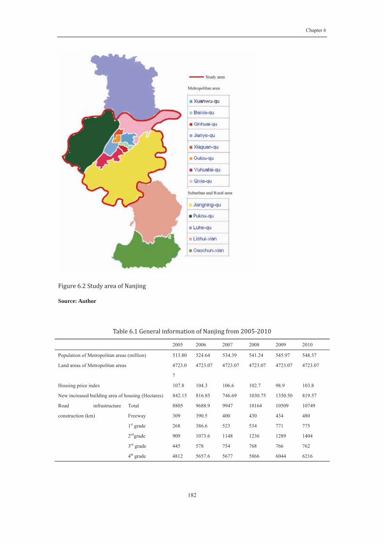
Chapter 6

182

Source: Author

2005 2006 2007 2008 2009 2010

Population of Metropolitan areas (million) 513.80 524.64 534.39 541.24 545.97 548.37

Land areas of Metropolitan areas 4723.0

7

4723.07 4723.07 4723.07 4723.07 4723.07

Housing price index 107.8 104.3 106.6 102.7 98.9 103.8

New increased building area of housing (Hectares) 842.15 816.85 746.69 1030.75 1350.50 819.57

Road infrastructure

construction (km)

Total 8805 9688.9 9947 10164 10509 10749

Freeway 309 390.5 400 430 434 480

1st grade 268 386.6 523 534 771 775

2ndgrade 909 1073.6 1148 1236 1289 1404

3rd grade 445 578 754 768 766 762

4th grade 4812 5657.6 5677 5866 6044 6216

Chapter 6

183

6.4.2 Data sources

Panel data at micro level are very rare even in industrial countries, because it has to be

collected repeatedly for the same individual over time. This is why the panel data

employed in this study is collected from a survey conducted by author. There are two

main components of this survey: urban morphology (street network) maps and both

property value and property’s attributes from 2005 to 2010.

6.4.2.1 Street network maps

The street network raw data of Nanjing Metropolitan areas from 2005 and 2010was

collected from a Chinese GPS map company. As the digital map they used is for Sat

Nav purposes, it has accurate street network information with proper geo-coordinates

for each year, so that it can capture accurate dynamic changes of the urban street

network within the metropolitan area. Figure (6.3) shows the street network changes

within each administration area by overlapping a time series of six annual maps. From

the composite map, it is seen how infrastructure construction re-shapes the urban

street layout in a very short space of time; for example, Hexi and Jiangning new town

developments in 2006, interior ring way construction in 2005, Nanjing Yangzi River

Third Bridge in 2006 and Xuanwu lake tunnel in 2006.

Sour

6.4.

Ano

prio

synt

in th

for

atta

segm

rce: Author

.2.2 Street n

other data so

or experienc

tax connect

he evolving

the street n

ched to in

ment neares

network an

ource is a sp

ce, I specify

tivity zones

g urban stree

network map

ndividual re

st to the ob

nalysis

pace syntax

y 10 ranges

. In order to

et layout, sp

ps from 200

esidential h

servation. F

184

x analysis o

of radii fro

o capture th

pace syntax

05 to 2010.

house price

Furthermore

f these stree

om 800m to

he dynamics

x analysis w

Also note

e observatio

e, spatial an

et network m

o infinite di

s of accessib

was administ

that the acc

on is the v

nalysis is al

Cha

maps. Base

istance as sp

bility conta

tered separa

cessibility v

value of s

lso employe

apter 6

d on

pace

ained

ately

value

treet

ed to

Chapter 6

185

calculate straight-line distance to the CBD (XinJie Kou), distance to the XuanWu lake and

distance to the ZhongShan park.

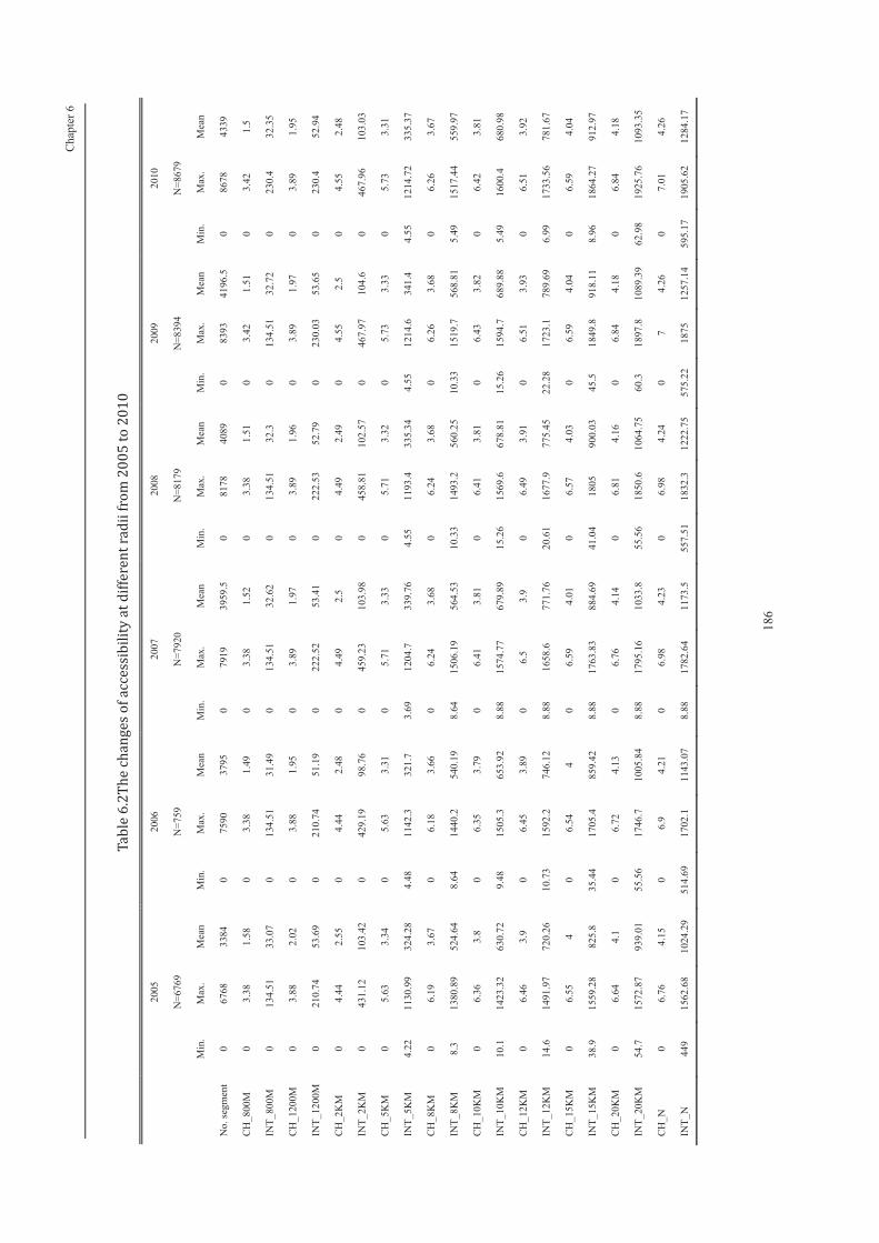
Cha

pter

6

186

2005

N=6

769

2006

N=7

59

2007

N=7

920

2008

N=8

179

2009

N=8

394

2010

N=8

679

Min

. M

ax.

Mea

n M

in.

Max

. M

ean

Min

. M

ax.

Mea

n M

in.

Max

. M

ean

Min

. M

ax.

Mea

n M

in.

Max

. M

ean

No.

segm

ent

0 67

68

3384

0

7590

37

95

0 79

19

3959

.5

0 81

78

4089

0

8393

41

96.5

0

8678

43

39

CH

_800

M

0 3.

38

1.58

0

3.38

1.

49

0 3.

38

1.52

0

3.38

1.

51

0 3.

42

1.51

0

3.42

1.

5

INT_

800M

0

134.

51

33.0

7 0

134.

51

31.4

9 0

134.

51

32.6

2 0

134.

51

32.3

0

134.

51

32.7

2 0

230.

4 32

.35

CH

_120

0M

0 3.

88

2.02

0

3.88

1.

95

0 3.

89

1.97

0

3.89

1.

96

0 3.

89

1.97

0

3.89

1.

95

INT_

1200

M

0 21

0.74

53

.69

0 21

0.74

51

.19

0 22

2.52

53

.41

0 22

2.53

52

.79

0 23

0.03

53

.65

0 23

0.4

52.9

4

CH

_2K

M

0 4.

44

2.55

0

4.44

2.

48

0 4.

49

2.5

0 4.

49

2.49

0

4.55

2.

5 0

4.55

2.

48

INT_

2KM

0

431.

12

103.

42

0 42

9.19

98

.76

0 45

9.23

10

3.98

0

458.

81

102.

57

0 46

7.97

10

4.6

0 46

7.96

10

3.03

CH

_5K

M

0 5.

63

3.34

0

5.63

3.

31

0 5.

71

3.33

0

5.71

3.

32

0 5.

73

3.33

0

5.73

3.

31

INT_

5KM

4.

22

1130

.99

324.

28

4.48

11

42.3

32

1.7

3.69

12

04.7

33

9.76

4.

55

1193

.4

335.

34

4.55

12

14.6

34

1.4

4.55

12

14.7

233

5.37

CH

_8K

M

0 6.

19

3.67

0

6.18

3.

66

0 6.

24

3.68

0

6.24

3.

68

0 6.

26

3.68

0

6.26

3.

67

INT_

8KM

8.

3 13

80.8

9 52

4.64

8.

64

1440

.2

540.

19

8.64

15

06.1

9 56

4.53

10

.33

1493

.2

560.

25

10.3

3 15

19.7

56

8.81

5.

49

1517

.44

559.

97

CH

_10K

M

0 6.

36

3.8

0 6.

35

3.79

0

6.41

3.

81

0 6.

41

3.81

0

6.43

3.

82

0 6.

42

3.81

INT_

10K

M

10.1

14

23.3

2 63

0.72

9.

48

1505

.3

653.

92

8.88

15

74.7

7 67

9.89

15

.26

1569

.6

678.

81

15.2

6 15

94.7

68

9.88

5.

49

1600

.4

680.

98

CH

_12K

M

0 6.

46

3.9

0 6.

45

3.89

0

6.5

3.9

0 6.

49

3.91

0

6.51

3.

93

0 6.

51

3.92

INT_

12K

M

14.6

14

91.9

7 72

0.26

10

.73

1592

.2

746.

12

8.88

16

58.6

77

1.76

20

.61

1677

.9

775.

45

22.2

8 17

23.1

78

9.69

6.

99

1733

.56

781.

67

CH

_15K

M

0 6.

55

4 0

6.54

4

0 6.

59

4.01

0

6.57

4.

03

0 6.

59

4.04

0

6.59

4.

04

INT_

15K

M

38.9

15

59.2

8 82

5.8

35.4

4 17

05.4

85

9.42

8.

88

1763

.83

884.

69

41.0

4 18

05

900.

03

45.5

18

49.8

91

8.11

8.

96

1864

.27

912.

97

CH

_20K

M

0 6.

64

4.1

0 6.

72

4.13

0

6.76

4.

14

0 6.

81

4.16

0

6.84

4.

18

0 6.

84

4.18

INT_

20K

M

54.7

15

72.8

7 93

9.01

55

.56

1746

.7

1005

.84

8.88

17

95.1

6 10

33.8

55

.56

1850

.6

1064

.75

60.3

18

97.8

10

89.3

962

.98

1925

.76

1093

.35

CH

_N

0 6.

76

4.15

0

6.9

4.21

0

6.98

4.

23

0 6.

98

4.24

0

7 4.

26

0 7.

01

4.26

INT_

N

449

1562

.68

1024

.29

514.

69

1702

.1

1143

.07

8.88

17

82.6

4 11

73.5

55

7.51

18

32.3

12

22.7

557

5.22

18

75

1257

.14

595.

17

1905

.62

1284

.17

Chapter 6

187

6.4.2.3 House prices and attributes

The analyzed data includes average selling price by spatial unit (residential project)

from 2005 to 2010 in Nanjing and was collected by the author from two Chinese

professional real estate website databases (www.sofun.com and www.fangjia.com).

The dataset includes for each project: information on the average selling price of

developments (ASP), the date of valuation, administration area, project units size,

gross-area, parcel-size, dummy variable of new blank of decoration, plot ratio, green

ratio, numbers of parking units and service maintenance fee. Although the survey

collected the ASP of individual residential development projects repeatedly from 2005

to 2010,there is still a missing data issue, due to missing attribute value and ASP for

some projects. The dataset is unbalanced in terms of sample size by each year, which

is not equal. There are 229 observations of projects in 2005 and observations of

projects increase to 592 in 2010, showed in table (6.3). This is because some projects

are newly developed and they do not have historical ASP. There are 2704 valid

observations in the study. The sample was not randomly selected, but the sample size

is more than 90% of the population within the metropolitan area. Furthermore, it was

commodity residential housing developments with simplex residential land use (flats)

that were also selected for observation, with developments with mixed land use and

affordable housing excluded from the study. The ASP recorded is the instant ASP in

October of each year. According to experience, October is the peak time for

transaction for the whole year, so the ASP in that month is a good indicator of supply

and demand.

2005 2006 2007 2008 2009 2010

N=229 N=308 N=447 N=540 N=588 N=592

5047.65 6096.64 7684.15 9292.93 11131.74 15073.59

Chapter 6

188

The dependent variables require more discussion. Most hedonic price studies use

individual house transaction price as the dependent variable to measure people’s

wiliness to pay extra money for the specific characteristics in the hedonic model.

However, this study applies average selling price, estimated by the developer, instead

of using the housing transaction price that is used in most hedonic price studies. There

are several pragmatic reasons for using the average selling price. Firstly, in mainland

China, transaction price information for new build sales is mainly controlled by

government, and is not released to the public. The registration systems for sales of

new houses and second-hand houses are in separate departments, and it is very

difficult to gain public access to the records of individual dwelling units. Secondly,

the Chinese housing market is not mature, as private property has been

commercialized only since1998, and there are few cases of properties transacted more

than two times. This means that even if historical transaction price data were available,

it would not be possible to construct a panel data set of transaction prices for the

purposes of our study. I have therefore chosen to take average selling price as a

surrogate and accept the noise that this inevitably introduces into the model.

Average selling price (yuan/m2) is the average price of a residential project for the

first transaction between developer and house purchasers. Because of the way the

residential development market works in China, this metric is a commonly understood

indicator of market performance. In the Chinese housing market, ASP is calculated by

real estate developers weekly or monthly, to measure housing demand and supply,

along with constructions cost and profits, and is an important reference for house

purchaser in understanding the dynamic of the market. Although the average selling

price is an advertised price, according to developer’s expectation, it is also used to

guide government taxation. According to research by Tian (2006), the formula of

average selling price is:

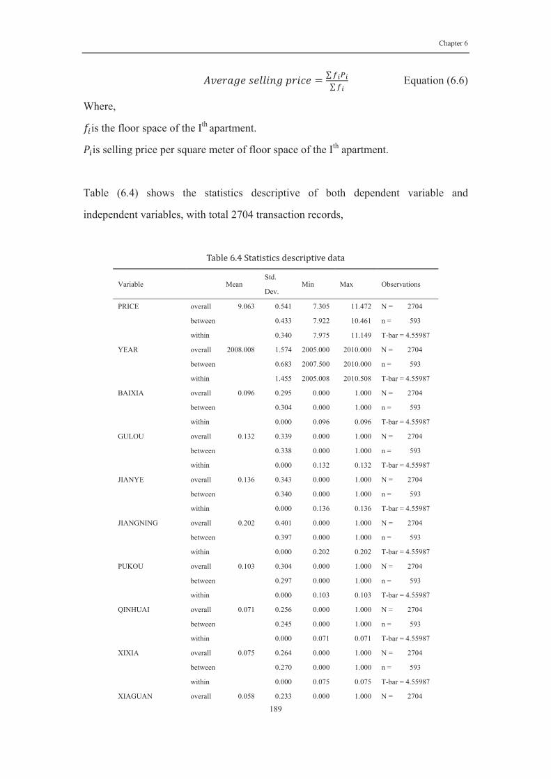
Chapter 6

189

Equation (6.6)

Where,

is the floor space of the Ith apartment.

is selling price per square meter of floor space of the Ith apartment.

Table (6.4) shows the statistics descriptive of both dependent variable and

independent variables, with total 2704 transaction records,

Variable Mean Std.

Dev. Min Max Observations

PRICE overall 9.063 0.541 7.305 11.472 N = 2704

between 0.433 7.922 10.461 n = 593

within 0.340 7.975 11.149 T-bar = 4.55987

YEAR overall 2008.008 1.574 2005.000 2010.000 N = 2704

between 0.683 2007.500 2010.000 n = 593

within 1.455 2005.008 2010.508 T-bar = 4.55987

BAIXIA overall 0.096 0.295 0.000 1.000 N = 2704

between 0.304 0.000 1.000 n = 593

within 0.000 0.096 0.096 T-bar = 4.55987

GULOU overall 0.132 0.339 0.000 1.000 N = 2704

between 0.338 0.000 1.000 n = 593

within 0.000 0.132 0.132 T-bar = 4.55987

JIANYE overall 0.136 0.343 0.000 1.000 N = 2704

between 0.340 0.000 1.000 n = 593

within 0.000 0.136 0.136 T-bar = 4.55987

JIANGNING overall 0.202 0.401 0.000 1.000 N = 2704

between 0.397 0.000 1.000 n = 593

within 0.000 0.202 0.202 T-bar = 4.55987

PUKOU overall 0.103 0.304 0.000 1.000 N = 2704

between 0.297 0.000 1.000 n = 593

within 0.000 0.103 0.103 T-bar = 4.55987

QINHUAI overall 0.071 0.256 0.000 1.000 N = 2704

between 0.245 0.000 1.000 n = 593

within 0.000 0.071 0.071 T-bar = 4.55987

XIXIA overall 0.075 0.264 0.000 1.000 N = 2704

between 0.270 0.000 1.000 n = 593

within 0.000 0.075 0.075 T-bar = 4.55987

XIAGUAN overall 0.058 0.233 0.000 1.000 N = 2704

Chapter 6

190

between 0.236 0.000 1.000 n = 593

within 0.000 0.058 0.058 T-bar = 4.55987

XUANWU overall 0.078 0.269 0.000 1.000 N = 2704

between 0.281 0.000 1.000 n = 593

within 0.000 0.078 0.078 T-bar = 4.55987

YUHUA overall 0.049 0.216 0.000 1.000 N = 2704

between 0.219 0.000 1.000 n = 593

within 0.000 0.049 0.049 T-bar = 4.55987

HOUSEHOLD overall 810.183 929.211 0.000 8000.000 N = 2704

between 901.578 0.000 8000.000 n = 593

within 0.000 810.183 810.183 T-bar = 4.55987

GROSS_BA overall 14.615 29.634 0.000 450.000 N = 2704

between 26.970 0.000 450.000 n = 593

within 0.000 14.615 14.615 T-bar = 4.55987

PACEL_S overall 9.564 21.158 0.000 300.000 N = 2704

between 19.612 0.000 300.000 n = 593

within 0.000 9.564 9.564 T-bar = 4.55987

DECORATION overall 0.090 0.287 0.000 1.000 N = 2704

between 0.286 0.000 1.000 n = 593

within 0.000 0.090 0.090 T-bar = 4.55987

NO_DECORATION overall 0.910 0.287 0.000 1.000 N = 2704

between 0.286 0.000 1.000 n = 593

within 0.000 0.910 0.910 T-bar = 4.55987

PLOT_R overall 2.353 2.204 0.290 28.400 N = 2704

between 2.221 0.290 28.400 n = 593

within 0.000 2.353 2.353 T-bar = 4.55987

GREEN_R overall 0.406 0.163 0.000 4.000 N = 2704

between 0.156 0.000 3.100 n = 593

within 0.060 -2.294 1.306 T-bar = 4.55987

PARKIN~N overall 549.599 724.059 0.000 9600.000 N = 2704

between 693.087 0.000 9600.000 n = 593

within 0.000 549.599 549.599 T-bar = 4.55987

SERVICECOST overall 1.796 9.407 0.000 200.000 N = 2704

between 8.230 0.000 200.000 n = 593

within 0.000 1.796 1.796 T-bar = 4.55987

CH_800M overall 1.123 0.916 0.000 3.159 N = 2704

between 0.906 0.000 3.159 n = 593

within 0.219 -0.763 2.988 T-bar = 4.55987

Int_800M overall 26.556 20.085 0.000 110.896 N = 2704

between 20.533 0.000 109.923 n = 593

within 3.336 -0.613 81.673 T-bar = 4.55987

CH_1200M overall 1.710 0.990 0.000 3.609 N = 2704

between 0.984 0.000 3.609 n = 593

within 0.268 -0.272 3.913 T-bar = 4.55987

Chapter 6

191

Int_1200M overall 45.818 38.459 0.000 225.211 N = 2704

between 39.664 0.000 219.794 n = 593

within 5.627 -5.382 97.018 T-bar = 4.55987

CH_2KM overall 2.378 1.102 0.000 4.353 N = 2704

between 1.107 0.000 4.348 n = 593

within 0.291 0.108 5.062 T-bar = 4.55987

Int_2KM overall 94.781 82.232 0.000 458.834 N = 2704

between 84.512 0.000 457.025 n = 593

within 9.488 16.944 152.862 T-bar = 4.55987

CH_5KM overall 3.372 1.383 0.000 5.549 N = 2704

between 1.388 0.000 5.546 n = 593

within 0.388 0.096 7.062 T-bar = 4.55987

Int_5KM overall 347.858 248.767 4.861 1200.282 N = 2704

between 254.354 4.861 1192.670 n = 593

within 27.734 55.974 481.674 T-bar = 4.55987

CH_8KM overall 3.748 1.520 0.000 6.101 N = 2704

between 1.518 0.000 6.095 n = 593

within 0.449 0.011 7.928 T-bar = 4.55987

Int_8KM overall 598.556 344.517 5.491 1503.338 N = 2704

between 349.923 5.491 1494.876 n = 593

within 44.854 164.825 804.564 T-bar = 4.55987

CH_10KM overall 3.894 1.578 0.000 6.278 N = 2704

between 1.570 0.000 6.272 n = 593

within 0.477 -0.029 8.220 T-bar = 4.55987

Int_10KM overall 731.524 371.984 5.491 1595.801 N = 2704

between 376.150 5.491 1584.911 n = 593

within 54.704 180.075 924.251 T-bar = 4.55987

CH_12KM overall 4.005 1.615 0.000 6.378 N = 2704

between 1.605 0.000 6.369 n = 593

within 0.499 -0.279 8.443 T-bar = 4.55987

Int_12KM overall 841.348 383.721 6.995 1683.363 N = 2704

between 386.375 6.995 1666.133 n = 593

within 63.160 209.702 1044.529 T-bar = 4.55987

CH_15KM overall 4.121 1.664 0.000 6.513 N = 2704

between 1.650 0.000 6.504 n = 593

within 0.526 -0.332 8.613 T-bar = 4.55987

Int_15KM overall 972.804 372.772 8.961 1809.427 N = 2704

between 373.027 8.961 1789.510 n = 593

within 71.336 279.579 1220.005 T-bar = 4.55987

CH_20KM overall 4.238 1.719 0.000 6.779 N = 2704

between 1.699 0.000 6.769 n = 593

within 0.559 -0.650 8.736 T-bar = 4.55987

Int_20KM overall 1126.919 331.764 102.371 1914.174 N = 2704

between 327.436 132.767 1885.313 n = 593

Chapter 6

192

within 82.454 408.373 1454.174 T-bar = 4.55987

CH_N overall 4.289 1.818 0.000 6.965 N = 2704

between 1.785 0.000 6.954 n = 593

within 0.594 -0.986 9.588 T-bar = 4.55987

Int_N overall 1260.245 249.667 554.104 1902.368 N = 2704

between 233.892 587.327 1861.653 n = 593

within 91.787 569.353 1532.228 T-bar = 4.55987

DIST_CBD overall 8.626 0.754 5.441 10.620 N = 2704

between 0.782 5.441 10.620 n = 593

within 0.000 8.626 8.626 T-bar = 4.55987

DIST_LAKE overall 8.844 0.579 6.900 10.659 N = 2704

between 0.594 6.900 10.659 n = 593

within 0.000 8.844 8.844 T-bar = 4.55987

DIST_PARK overall 9.089 0.432 7.681 10.561 N = 2704

between 0.439 7.681 10.561 n = 593

within 0.000 9.089 9.089 T-bar = 4.55987

6.5 Analysis and empirical results

6.5.1 Street network analysis

Chapter 6

193

Source: author

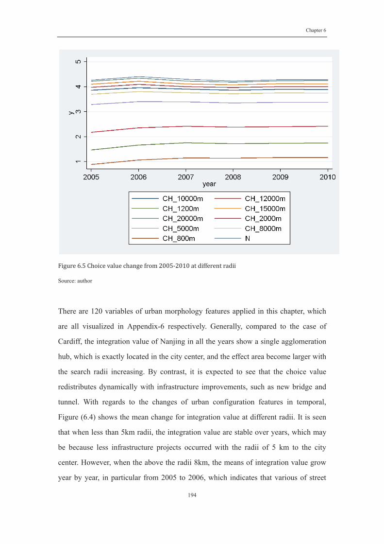
Chapter 6

194

Source: author

There are 120 variables of urban morphology features applied in this chapter, which

are all visualized in Appendix-6 respectively. Generally, compared to the case of

Cardiff, the integration value of Nanjing in all the years show a single agglomeration

hub, which is exactly located in the city center, and the effect area become larger with

the search radii increasing. By contrast, it is expected to see that the choice value

redistributes dynamically with infrastructure improvements, such as new bridge and

tunnel. With regards to the changes of urban configuration features in temporal,

Figure (6.4) shows the mean change for integration value at different radii. It is seen

that when less than 5km radii, the integration value are stable over years, which may

be because less infrastructure projects occurred with the radii of 5 km to the city

center. However, when the above the radii 8km, the means of integration value grow

year by year, in particular from 2005 to 2006, which indicates that various of street

Chapter 6

195

network improvements enhanced the city connectivity, especially the urban suburb

area. Relatively, choice value shows two types of changes trend, in particular during

the period of 2005 to 2007 (Figures 6.5). Within the radii of 2km , the mean of the

choice value increase, whereas, all average choice value decrease slightly when above

the radii of 5 km, which implies that the series of main road improvements have

brought relief to the congestion. In that case, the traffic flows increased in the areas

surrounding the center and is reduced in the area of suburb area.

6.5.2 Empirical results

Bearing in mind that the objective of this study is to examine the micro-dynamic

effect of street network configuration on housing price using a panel model. There are

five forms of models employed in this study: pooled model, individual-fixed effect

model, random effect model, time-fixed model and two-ways effect fixed model, all

using average selling price as the dependent variable and 40 explanatory variables,

including 20 urban configuration attributes and 20 time-invariance attributes (e.g.

distance to CBD, project units size, gross-area, parcel-size, decoration condition, plot ratio,

green ratio, parking units size and service maintenance fee). As mentioned in the

methodology section, the fixed effects model can control for time invariance by

absorbing time invariant variables in the intercept. The random effect model deals

with time invariant components as explanatory variables. Thus, the time-invariance

attributes are excluded in individual-fixed effect model, time-fixed model and

two-way effect model. The exploratory process of panel analysis will be decomposed

into seven components, which are as follows:

Variables OLS Fixed Random Time-fixed Two-ways

Ceof. t value Ceof. t value Ceof. t value Ceof. t value Ceof. t value

Intercept 10.055 23.559 ** 10.868 16.594 **

CH_800M -0.009 -0.385 0.083 2.138* 0.032 1.083 0.001 0.054 -0.002 -0.063

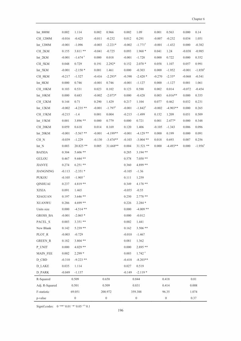
Chapter 6

196

Int_800M 0.002 1.114 0.002 0.966 0.002 1.09 0.001 0.563 0.000 0.14

CH_1200M -0.016 -0.425 -0.011 -0.232 0.012 0.291 -0.007 -0.232 0.034 1.051

Int_1200M -0.001 -1.096 -0.003 -2.221* -0.002 -1.771# -0.001 -1.432 0.000 -0.382

CH_2KM 0.155 3.811 ** -0.041 -0.725 0.093 1.968 * 0.041 1.24 -0.038 -0.985

Int_2KM -0.001 -1.674 # 0.000 0.018 -0.001 -1.728 0.000 0.722 0.000 0.352

CH_5KM 0.048 0.729 0.191 2.292* 0.152 2.070 * 0.058 1.107 0.057 0.991

Int_5KM -0.001 -2.150 * 0.001 1.461 0.000 -0.303 0.000 -1.952 -0.001 -1.858#

CH_8KM -0.217 -1.527 -0.416 -2.293* -0.390 -2.420 * -0.270 -2.33* -0.068 -0.541

Int_8KM 0.000 0.746 -0.001 0.746 -0.001 -1.127 0.000 -1.127 0.001 1.061

CH_10KM 0.103 0.531 0.023 0.102 0.123 0.588 0.002 0.014 -0.072 -0.454

Int_10KM 0.000 0.683 -0.002 -2.073* 0.000 -0.428 0.003 6.016** 0.000 0.355

CH_12KM 0.144 0.71 0.290 1.429 0.217 1.104 0.077 0.462 0.032 0.231

Int_12KM -0.002 -4.235 ** -0.001 -1.797# -0.001 -1.842# -0.002 -4.903** 0.000 0.265

CH_15KM -0.215 -1.4 0.001 0.004 -0.215 -1.499 0.152 1.209 0.051 0.509

Int_15KM 0.001 3.896 ** 0.000 0.779 0.000 0.721 0.001 2.477* 0.000 0.348

CH_20KM 0.059 0.618 0.014 0.169 0.120 1.406 -0.105 -1.343 0.006 0.096

Int_20KM -0.001 -5.567 ** -0.001 -4.199** -0.001 -4.129 ** 0.000 0.199 0.000 0.091

CH_N -0.039 -1.229 -0.130 -3.474** -0.103 -3.004 ** 0.018 0.693 0.007 0.256

Int_N 0.003 20.825 ** 0.005 31.668** 0.004 31.521 ** 0.000 -4.493** 0.000 -1.956#

BAIXIA 0.304 5.606 ** 0.285 3.194 **

GULOU 0.467 9.444 ** 0.578 7.050 **

JIANYE 0.274 6.251 ** 0.360 4.899 **

JIANGNING -0.113 -2.351 * -0.105 -1.36

PUKOU -0.105 -1.905 # 0.111 1.259

QINHUAI 0.237 4.819 ** 0.349 4.178 **

XIXIA 0.091 1.465 -0.055 -0.55

XIAGUAN 0.197 3.646 ** 0.250 2.778 **

XUANWU 0.286 4.699 ** 0.226 2.284 *

Units size 0.000 -4.514 ** 0.000 -4.009 **

GROSS_BA -0.001 -2.065 * 0.000 -0.012

PACEL_S 0.003 3.351 ** 0.002 1.441

New Blank 0.142 5.239 ** 0.162 3.506 **

PLOT_R -0.003 -0.729 -0.010 -1.467

GREEN_R 0.182 3.804 ** 0.081 1.362

P_UNIT 0.000 4.029 ** 0.000 2.895 **

MAIN_FEE 0.002 2.299 * 0.003 1.742 #

D_CBD -0.310 -9.223 ** -0.418 -8.203**

D_LAKE 0.035 1.114 0.027 0.519

D_PARK -0.049 -1.137 -0.149 -2.119 *

R-Squared 0.509 0.658 0.844 0.418 0.01

Adj. R-Squared 0.501 0.509 0.831 0.414 0.008

F-statistic 69.051 200.972 359.388 96.35 1.074

p-value 0 0 0 0 0.37

Signif.codes: 0 ‘**’ 0.01 ‘*’ 0.05 ‘#’ 0.1

Chapter 6

197

Firstly, ordinary least squares (OLS) was performed for pooled regression models,

assuming the coefficients for any individual at any cross-section do not vary in time.

The tests for the OLS model in figure (6.5), shows that Adj.-R-Squared is 0.501, F test

is 69.051, and the p value is 0.000, which indicates that the model is statistically

significant. There is a linear dynamic relationship between street configuration

accessibility and housing price with 40.6% variance explained by this model. With the

exception of three areas, namely XIXIA,PUKOU and JIANGNING, the T scores of

all others areas are above 1.96 with a positive sign, which indicates the relationship

between accessibility and housing price in these areas is stable over the years.

Furthermore, as expected, distance to CBD ,project units size and gross-building area

are significant, all with negative signs, whereas parcel size, decoration status, green

space ratio, numbers of parking spaces, and service cost are significant with positive

signs. These findings suggest that projects nearer to the CBD, with fewer households,

bigger parcel size, good decoration, more green space, more parking space and high

service cost (indicating better/more club goods) are associated with higher price.

In terms of urban configurational attributes, the space syntax choice (betweenness)

coefficient only has a significant (positive) impact at radii 2km. This implies that the

locations of greatest people movement measured within 2km travel distance is

associated with higher house prices. This may be picking up local agglomeration

effects at a neighborhood level, with highest movement potential from a 2km

catchment generating sufficient neighborhood economies of scale to attract

home-value enhancing facilities, possibly including metro stations.

By contrast, the integration(closeness) value, measuring access to opportunities,

shows a significantly negative impact at radii 5km, 12km and 20km, but positive

impact at15km and N km. This apparently arbitrary pattern seems to indicate that high

value property is found in a mix of less and more accessible places. There is a

Chapter 6

198

non-monotonic relationship between closeness and house price but there are

significant relationships between house price and specific levels of closeness. It is

difficult to think of specific explanations for these patterns, but it must be a function

of the particular configuration of Nanjing and its recent extensions. One explanation

might be that 5, 12 and 20km radii do not correspond to significant search areas for

any particular kind of destinations demanded by higher income residents – on the

contrary, they may correspond to search areas for low-paid jobs, which would account

for the negative coefficients. It might also be noted that the global integration value

has the largest T score (20.825), reflecting the fact that most high value projects are

located at places that are easy to access from across the city. In Nanjing as elsewhere,

people pay for accessibility to transaction opportunities at different scales.

Next, I performed a fixed effects model (also known as individual-fixed), which

allows that unobserved heterogeneity between individual project prices to vary across

space, while parameters are constant. Table (6.5), shows that the model is

statistically significant (p<0.05) and adj.-R-Squared is 0.509, confirming that a

dynamic relationship between street network improvement and housing price exists.

In the fixed effects model, the space syntax choice (betweenness) values, indicating

the relative level of traffic flow in street segment, are significant at radii 800m and

5km with positive signs, and also significant at radii 8km and N km with negative

signs. This is again suggesting interesting subtle patterns in the spatial economy:

within 5km area, the high value properties are located near main streets where the

pedestrian flows are high. 800m betweenness hotspots are attractive places to live by

virtue of access to a high density of local walking-based destinations. Betweenness

hotspots at 8km and N km have high traffic externalities that are not compensated for

by local services.

On the other hand, as the p-values of integration (closeness) values measured at radii

1200m, 10km and 20kmarelower than 0.05, and the all of their T-tests are negative,

Chapter 6

199

there is evidence that some at least of the high value properties are not located at

easily accessed place, such as near highways and elevated roads. This may well reflect

the phenomenon of high valued exclusive gated developments on the urban periphery.

Nevertheless, the more significant pattern is for high value properties to be located at

places of easy access, with the t value of global integration being largest of all.

Based on the results of the individual-fixed effect model, it can be inferred that street

network improvements at a small scale (e.g. improving street density and

development of small new-town developments), tend to add value to residential

projects, whereas larger scale street network improvement (e.g. freeways, express

ways and bridges) tend to impose negative externalities(noise, fumes and insecurity)

on housing, which are capitalized in asking price. Furthermore, the results also

confirm the benefit to housing price from both inner and outer ring roads, as these

decentralize the street connectivity from the original city center, adding value to

properties further out.

F test for individual effects

F = 9.5741 df1 = 573 df2 = 2090 p-value < 2.2e-16

alternative hypothesis: significant effects

The third step is to test whether the panel model controls the unobserved determinants

efficiently. If the fixed model is better than the OLS model, we should use the panel

structure, otherwise the pooled model should be used. A simple Chow test is used to

check whether the fixed model is significantly different to the OLS model, showed in

table (6.6). If the p-value is < 0.05 then the fixed effects model is a better choice. In

this case, as the p-value is much lower than 0.05, we can reject the null hypothesis

and choose the fixed model.

Chapter 6

200

The fourth step is to run a random effects model. The crucial distinction between

fixed and random effects is whether the unobserved individual effects embody

elements that are correlated with the regressors in the model (Greene 2008). As table

(6.5) shows, the Random effects model is also significant with a much higher

adj.-R-Squared: 83.1% of variation being explained by this model.

Looking at the time-invariant variables, the dummy variables for five admin areas are

found to be significant at 95% confidence: BAIXIA, GULOU, JIANYE, QINHUAI

and XIAGUAN, which is to be expected: Figure (6.3) clearly shows the larger

numbers of street network improvements in these administration areas, which have

attracted private estate developers to develop luxury residential projects for

high-income people as the location became more accessible. This is particularly

strong in the GULOU area. Furthermore, the variable ‘unit size’ is significant at 99%

level with a negative sign, whereas decoration condition is significant with a positive

sign and number of parking spaces is also significant with a positive impact on house

prices. This implies that projects in the high-end market have the characteristics of

lower density, better decoration and more parking space near the city center, whereas

the projects for the general market are associated with large numbers of units, new

blank decoration and less parking space.

In addition, it was found that the attributes of total building area, parcel size, plot-ratio

and green ratio are not significant statistically, indicating interestingly that high value

of ASP are not related to development density. As expected, both the distance to CBD

and distance to a major park are significant with a negative sign, but the variable of

distance to lake dropped out of the model. This may be due to the fact that although

the lake is free for public, it is gated and there are only six entrances. Thus the

XUANHU lake appears to have no spillover effect on house prices.

In terms of urban morphology attributes, betweenness (choice) value at radii 2km and

Chapter 6

201

5km are significant with a positive sign, and the choice values at radii 8km and globe

are significant with negative sign. As I have already suggested when discussing the

other models, this shows distinctive spatial boundaries for different kinds of demand.

Within 5km area, high pedestrian flows have a positive externality on housing price,

since they imply higher vitality and more welfare-enhancing destinations catering for

foot-born custom. Higher betweenness over 5km is associated with higher automobile

traffic and associated negative externalities.

Integration values are statistically significant only at radii 20km and globally, with

different signs, underlining the existing of submarkets. As has already been noted,

many high value properties are located in places less accessible within radii 20km, but

some types of such developments buck this trend in the urban fridge area.

Hausman Test

chisq = 1029.051 df = 20 p-value < 2.2e-16

alternative hypothesis: one model is inconsistent

The next step is to choose between the fixed effect model and the random effects

model. As noted in the methodology section, the fixed effects model only describes

the relationship within selected samples, while the random effects model could be

interpreted to larger populations. The Hausman-Wu test (Hausman, 1978) was

employed to make the choice, based on whether the unobserved individual effects

elements are correlated with the repressors in the model. If the p-value is significant

(for example <0.05) then the fixed effects model should be used(Greene 2008).From

table (6.7), the chi-sq is 1029.051 and p-value is lower than 0.05, so the fixed effect

model is better than the random model.

The sixth step is to examine the relationship by time-fixed-effects model, which

Chapter 6

202

allows unobserved heterogeneity (e.g. inflations and mortgage rate) to vary only

across time, and ignores the heterogeneity of individuals across space. If the model is

significant statistically, it indicates that the rate of price change for the whole market

for each year is not equal.

The model turns out to be statistically significant, with an adj.-R-Squared of 0.414

and F test of 96.350, showed in table (6.6), which indicate that the price change rate

of the whole market for each year is different. Compared with the performance of

urban configurational attributes in the individual-effect model, it is found that

integration or choice values are hardly significant within the radii at 5km, which

suggest that the housing price volatility within the old town has little relationship with

the change of urban configuration statistically. This is as expected, as few large size

street layout improvements occurred in the old town during the study periods, as seen

in figure (6.3). However, the Choice value is significant at radii 8km with a negative

sign, indicating that within the specific area of people’s travel distance range (between

5km-8km), property value increased in some location where the choice value

decreased during 2005 to 2010. The reasons may be that the specific area is located in

an area where the old town and the new town intersected, and normally the ring road

and expressways are the means to link the old and new town. After these links had

been constructed, people started to choose the ring road or express way for minimum

travel time, so that the original choice value decreases, as traffic volume are mainly

shifted to the ring road and express ways.

Integration values are significant at radii 12km and globally with negative t values,

while 10km and 15km integration values have positive signs. This implies that there

are two opposite relationships between housing price change and integration change

outside of the old town, and the ring road is the spatial boundary that divides these

two relationships. Since the ring road is located far from the city center at a network

integration distance of 10km and 12km. It is known that building the ring road could

Chapter 6

203

enhance central growth and allow people living in the suburb areas or city center to

quickly access both areas. Thus, house price increases are associated with integration

increases in suburb areas, new town and within the old town. However, regarding the

area within the inner ring road, the integration value is similar with choice value, and

has decreased in value since the ring road was constructed. The ring road enables

people to commute within the inner ring road, especially when two places are

positioned diagonally. The time-fixed model shows how housing price volatility is

also associated with spatial accessibility change across time and the results conform to

the dynamic relationship between housing price and street accessibility. This also

suggest that the relationship within the inner ring road is opposite to that beyond the

inner ring road. However, the time-fixed effect model cannot reflect how the volatility

of different markets (high-end or low-end) follows the changes of urban

configuration..

Thus, a chow test and Lagrange Multiplier Test were used to examine further whether

the data needs a two-way effect model, which allows the unobserved heterogeneities

to vary across both space and time (e.g. people’s expectation, housing stocks, and

business circumstance of each developer). The two-way effect model can be used to

examine whether the dynamic relationship over space is synchronous with that over

time, which means that a bigger price movement caused by a bigger change of spatial

accessibility can be found in the market of higher value property. The p-values of both

Chow test and Lagrange Multiplier Test are smaller than 0.05, showed in table (6.8)

and (6.9), which rejects the null hypothesis of no difference between individual-fixed

effect and time-fixed effect model. Hence, a two-way fixed-effect model should be

explored.

F test for individual effects

F = 5.323 df1 = 587 df2 = 2091 p-value < 2.2e-16

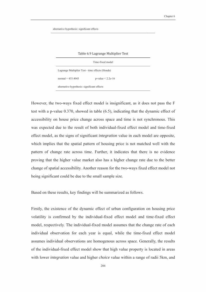
Chapter 6

204


Time-fixed model

Lagrange Multiplier Test - time effects (Honda)

normal = 433.4043 p-value < 2.2e-16


However, the two-ways fixed effect model is insignificant, as it does not pass the F

test with a p-value 0.370, showed in table (6.5), indicating that the dynamic effect of

accessibility on house price change across space and time is not synchronous. This

was expected due to the result of both individual-fixed effect model and time-fixed

effect model, as the signs of significant integration value in each model are opposite,

which implies that the spatial pattern of housing price is not matched well with the

pattern of change rate across time. Further, it indicates that there is no evidence

proving that the higher value market also has a higher change rate due to the better

change of spatial accessibility. Another reason for the two-ways fixed effect model not

being significant could be due to the small sample size.

Based on these results, key findings will be summarized as follows.

Firstly, the existence of the dynamic effect of urban configuration on housing price

volatility is confirmed by the individual-fixed effect model and time-fixed effect

model, respectively. The individual-fixed model assumes that the change rate of each

individual observation for each year is equal, while the time-fixed effect model

assumes individual observations are homogenous across space. Generally, the results

of the individual-fixed effect model show that high value property is located in areas

with lower integration value and higher choice value within a range of radii 5km, and

Chapter 6

205

that this distribution is stable over 5 years; whereas, in time-fixed effect model, it is

also found that the change of spatial accessibility can affect house price volatility. For

example, in urban suburbs, increasing integration can increase property value, and

within the ring road, decreasing choice value could also increase property value,

(choice value at 8km has a negative sign, and integration value at 10km and 15km has

a positive sign). Although the two-way effect model is insignificant, it also indicates

that housing price dynamics are asynchronous over space and time, and the rate of

price change seems more related to location than to property value per se.

Secondly, the dynamic relationship between urban configuration and housing price is

only valid for selected samples as the Hausman-Wu test rejected the null hypothesis,

suggesting that the individual –fixed effect model is better fitted to this dataset than a

random effect model.

Thirdly, the results imply the existence of housing submarkets as suggested, for

example, by the finding that the dynamic relationship between urban configuration

and housing price within the inner ring road is different from that beyond the inner

ring road. This in turn suggests a positive dynamic relationship in the suburb area and

a negative relationship in the buffer area.

6.6 Discussion

After the analysis, there are several points that need to be further discussed. Firstly,

compared with traditional measurement for accessibility, the space syntax method is

effective in capturing the accessibility changes at different levels of urban

configuration at a disaggregated level. As the theory suggests, change of accessibility

could be considered the most important geographical determinant of housing price

movements (Capozza and Helsley 1989), however, few studies can empirically prove

Chapter 6

206

this hypothesis. One of the difficulties is to measure the change of accessibility

accurately. For example, Iacono and Levinson (2011) conclude that the inappropriate

measurement of accessibility could be a reason for models to be insignificant.

However, this study confirms that the dynamic effect of urban configuration on

housing price volatility exists. This allows, with appropriate modeling tools, for

governments and investors to predict housing price pattern and movement by

observing the levels and changes of accessibility across time and space. However,

whether accessibility has a lagged effect on housing price still needs to be explored in

greater detail.

In addition, it is found that not all types of road infrastructure improvements add

value to the property, and people clearly have different preferences for road

connectivity and traffic flow in central urban areas and in suburbs. For example,

betweenness (choice) values tend to have positive signs at small radii, indicating

people’s willingness to pay extra money for intensely used streets within walking

distance due, I suggest, to agglomeration economy effects of local amenities, rather

than street segment connectivity per se. In contrast, a series of large scale street

network improvements has been implemented by the government, rendering the city

more accessible, but the evidence shows that it has a negative impact on people’s

private wealth and welfare, as both integration and choice show negative signs at

large radii and thus also negatively impact on the housing price. Consequently it is

possible to infer that people prefer high traffic flow in the central city and less

connectivity and traffic flow in suburb areas.

Thirdly, the significant space syntax attributes at different radii could reflect the

existence of housing neighborhood submarkets, and a dynamic relationship between

these submarkets. The results of the time-fixed effect model suggests that housing

price volatility is not affected by change of urban configuration in the city centre.

There is a negative relationship between urban configuration and housing price,

Chapter 6

207

mainly found in the area within the ring road within a 2km buffer distance. The

change of urban configuration stimulated house prices to increase in the area beyond

the ring road, This is because the improvement of the ring road enhanced the

connections between city center and suburbs. However, this also reduced the

connection and increased the traffic volume in a 2km buffer area round ring road, as

the two space syntax indices show a different sign at different radii. Furthermore, the

two-way effect model is insignificant, which implies that the price change rate of high

value property is not similarly high. Thus, the price change rate is related with

location rather than the property value. It can be concluded that with the benefit of

urban growth, house prices of submarkets in suburban areas are more likely to be

impacted by accessibility changes.

Finally, it can be noted when comparing this chapter with the previous one, that

people from different countries have different preferences, and different purchasing

characteristics with respect to the urban configurations of housing properties. As the

results of the Cardiff case showed in chapters 3and 4, high price property is associated

with high street connectivity and low traffic flow, and high-income people do not care

about how street segments connect and the state of traffic flow in suburb areas of the

UK. However, the Chinese study shows that high price property is associated with

high traffic flow in city center and both low connectivity and traffic flow in suburb

area. This may be due to the different life styles or travel behaviors resulting

indifferent preferences for urban configurations. Thus, it is suggested that further

studies are needed to explore the relationship between urban configuration and

housing price in different types of cities.

6.7 Summary

Despite the large numbers of studies exploring the relationship between location and

land value, there is still remarkably little evidence on how this relationship evolves

Chapter 6

208

over time and space. Furthermore, the traditional hedonic statistical methods and

hybrid repeat sale and hedonic methods fail to detect an accurate relationship over

time, especially when the unobserved heterogeneity varies over time, due to, for

instance housing policy and mortgage rate changes. The objective of this study was to

explore the geographical determinants of housing price movement at a city scale,

examining whether there is a dynamic effect of urban configuration on housing price

change by using a longitudinal analysis, which has typically been employed in studies

examining the determinants of house price volatility at a macro level. A

location-based social network analysis method, known as space syntax, was applied to

measure the accessibility contained in urban morphology. Then I conducted a survey,

collecting street network map data, housing values, and related attributes for the

metropolitan areas of Nanjing from 2005 to 2010.The statistical evidence suggests

that the accessibility information contained in an urban configuration network graph

is an important geographical determinant influencing housing price dynamics over

space and time, respectively. Dynamics caused by urban street network infrastructure

improvements have both positive and negative impacts on housing price overtime.

Generally, accessibility measured using closeness as the indicator across the

city(connectivity to everywhere else in the whole city) has a negative impact on prices.

The betweenness value has a positive impact on the city center and a negative impact

on the urban suburb. Furthermore, responding to changes of accessibility caused by

the construction of the ring way, there is a negative dynamic relationship within the

ring road and positive dynamic relationship beyond the ring road. But there is no

evidence to suggest that places with high accessibility also have a high change rate, as

the correlations is dependent on the particular case of urban morphology change in

each housing submarket.

Chapter 7

209

Chapter Seven:

Conclusions

7.1 Introduction

The focus of this thesis is on urban morphology and property markets. In particular, it

investigates the externalities of urban configuration on housing price, asking whether

households are more willing to pay extra for a more generally accessible location

when they purchase a property without a specific motivation and travel destination.

The purpose of this final chapter is to summarise the key findings of previous chapters.

It is divided into four sections. In addition, the chapter discusses policy implications

of the thesis findings, including the importance of the research with respect to the

hedonic price theory as well as the role of space syntax theory, and more generally

spatial network analysis, and as a method to aid the precision of government and

private sector planning and management of the built environment. I then comment on

the study’s limitation with respect to the issue of econometric estimation and the

handling of space syntax radii. The final section provides suggestions for how the

research can be further developed and will highlight directions for future research.

Finally, some final conclusions for this entire thesis are offered.

7.2 Conclusions for each chapter

Chapter two presented a literature review of hedonic price modeling, which can be

summarized from a number of aspects. Firstly, it is generally accepted in the literature

that under the conditions of a perfectly competitive market, where demand equals

supply, people’s willing to pay for each characteristic of property becomes the

Chapter 7

210

implicitly measured attribute of the hedonic price model. Existing economic theories

do not, however, provide clear guidelines on how to select hedonic price functional

form. Moreover, hedonic modeling also suffers from a number of econometrics issues,

which also lead to biased estimation, such as spatial heteroscedasticity, spatial

autocorrelation and multicollinearity. The rest of chapter two mainly focused on

reviewing relevant literature about locational attributes that have an impact on

housing price. It was noted from the literature that urban growth as well as polycentric

renders the urban system progressively more complex and that most people choose a

location without considering minimum travel cost to employment centre.

Consequently, the role of the distance to CBD in theory and in hedonic studies has

less impact than earlier theories suggest. Finally, I suggest that the methods of

measuring accessibility is overly simple as they mainly rely on the Euclidean distance

where as disaggregated measurements requires a prior specification of destinations. It

was also noted that by using Euclidean distance, even of polycentric centres, hedonic

modeling studies ignore the potentially rich source of information contained in a city’s

road grid pattern.

Chapter three presented the space syntax methodology and its underlying algorithms.

There are some inconsistencies in its early topological distance measurement, but a

series of improvement such as metric segment analysis and geometric angular cost

segment analysis, have improved the accuracy with which it measures general spatial

accessibility. The literature also implies that metric segment analysis is suitable for

large-scale analysis.

There are two mainly in dices used in space syntax metric segment analysis, both

measuring the accessibility contained in urban configuration. The first attribute is

integration (closeness) and the second is choice (betweenness). Integration can be

interpreted as how well connected or how close one street segment is to all other

street segment within the search radius. This measurement can indicate a proxy for the

Chapter 7

211

cost of overcoming spatial separation within a network of road segments. Choice can

indicate the pattern of movements through the network within a specific radius.

However, space syntax theory has not delineated the restrictive criterion on how to

specify a search radii, which depends on the researcher’s purpose and scale of study

objective. Thus, the specification of search radii for each empirical study is

pre-defined individually, usually in an exploratory fashion (ie without a priori

hypotheses) but also usually taking as a rule of thumb, the association of certain radial

distances with certain transport modes. In most cases radii are chosen for their

assumed association with people’s travel behavior by walking, cycling and vehicular

transport. Although there exist a large number of studiessuggesting that housing price

pattern is highly correlated with urban morphology, few studies test the hypothesis

that urban street network morphology is a fundamental geographical determinant of

house price (and therefore of the configuration of agglomeration externalities).

Chapter four therefore tests whether urban configuration can be a geographical

determinant of house prices at both disaggregated and aggregated level. It uses the

UK city of Cardiff as a case study. Compared to conventional geometrical measures

of accessibility, the results imply that a network approach to measuring accessibility

in urban areas improves the model’s performance with respect to explanatory power

and a reduction in heteroscedasticity, spatial autocorrelation and multi-collinearity.

Through estimating space syntax accessibility variables across a variety of spatial

scales, the chapter demonstrates that the study area displays a bi-centric urban

configuration with respect to property prices that corresponds to local and city-wide

externalities. The results show thaturban network configuration has a statistically

significant impact on house price at both aggregated and disaggregated levels.

Integration and choice both significantly affect house price for disaggregated data;

integration value has a positive impact on house price whereas choice value has a

negative impact. In regards to aggregated data, integration remains significantly

positively correlated with house price, whilst choice value becomes insignificant. Due

Chapter 7

212

to the particular pattern of the street network in the case study city of Cardiff, with

many dead-end streets linked directly to main streets, there is a higher variance for

choice. However, this is lost at the aggregate level. Finally, the experiment shows that

detailed urban configuration indicators measured from a network model of the urban

grid had a stronger power in explaining variances of the house prices than the

traditional measure of distance to CBD and without the scale limitation of that

measure.

Chapter five provides new knowledge addressing the lack of understanding on how to

deal with submarkets when the dwelling type is homogenous and neighbourhood

characteristics are unstable over time. This chapter showed that urban configurational

data recovered from a graph model of a street network adds significant explanation

power in distinguishing between housing sub-markets and thus provides a potentially

useful approach to analyzing sub-markets. This chapter used the same data set and

study area presented in Chapter four. The whole process of identifying housing

submarket followed the Schnare and Struyk procedure (1976), and compared the

efficiency of two new alternative specifications. The first specification is optimal

urban configuration and the second is nested urban configuration and building type

with two traditional spatial specifications. The results show that all specifications

using network metrics have significantly improved the estimation over and above the

market-wide model. Although the specifications based on urban configurational

features are not the best performing models, these results are quite close to the

traditional specifications. In particular, the new alternative specification seems more

objective, and less reliant on a housing market culture that has evolved around

distinctly different building types. This suggests that it may be particularly useful in

urban housing markets with a high degree of homogeneity in building type.

Furthermore, the results also imply that different socio-economic classes have

different preferences of urban morphology features. For example, people of the

middle class cohort or above in Cardiff, tend to live further away from the city centre

Chapter 7

213

since they have access to cars and consequently are less sensitive to how well street

segments are connected. This is in stark contrast to lower income people who seem

more sensitive to the geometrical pattern of street segments.

Chapter six applies a network approach to hedonic modeling in a housing market

dominated by simplex building types (Nanjing, China) and addresses the hypothesis

that there is a micro-dynamic relationship between urban morphology and house price.

It uses a large panel data set (of 2704 house prices) for the city of Nanjing, from 2005

to 2010. The statistical evidence suggests that the accessibility contained in urban

configuration is an important geographical determinant influencing the housing price

dynamic over space and time, respectively. Furthermore, urban street network

infrastructure improvements have both positive and negative impacts on housing price

over time. For example, integration has a negative impact on prices, while choice

value has a positive impact in the city center and a negative impact in the urban

suburb. This offers support for the idea that network metrics allow us to identify

housing submarkets defined at least partially in relation to particular morphological

characteristics – as predicted from the previous chapter. In particular, in the area

surrounding the ring road in Nanjing, there is a negative dynamic relationship inside

the ring road and a positive dynamic relationship beyond the ring road. However,

there is no evidence that places with high accessibility also have a high change rate.

The results imply that house prices in the suburbs are more likely to be effected by the

dynamics of urban configuration. By comparing the results in chapter four and five, it

is found that people from different countries have different preferences in regards to

the urban configurations of residential properties. For example, in the UK context,

high priced properties are associated with high street-connectivity and low traffic flow,

and high-income people do not apparently care about the connectivity of street

segments and the state of traffic flow in suburban areas of the UK. However, the

Chinese study shows that high price properties are associated with high traffic flow in

the city center and both low connectivity and low traffic flow in suburban areas.

Chapter 7

214

Source: author

In summary, this thesis attempts to contribute to the hedonic theory through its emphasis on housing

price mainly at the micro level (Figure 7.1), and provides a framework for the study of urban

morphology and housing market. Several empirical evidences show that the urban configurational

features can have both positive and negative impacts on property value. The spatial information

contained in the urban form has stronger explanations for the variance of housing price compared to the

information of traditional locational attributes, and be more objective. Surprisingly, this study also

found that urban configurational features are associated with structure characteristics and

neighborhoods characteristics, and that each social class has specific preferences in terms of building

type and street layout. Moreover, at the macro-level, it is known that the real estate is closely associated

with social, economic and policy factors, but from the urban planning perspective, the studies on urban

configuration may be a means to tackle some complex issues (e.g. social exclusion and housing

segregations) through efficient allocations of space, following this framework here.

Chapter 7

215

7.3 Implications

This section discusses the implications of these findings from three perspectives:

firstly, implications for the space syntax and related spatial network theory; secondly,

implications for hedonic house price research; and thirdly implications for urban

development and planning policy.

7.3.1 Implications for the Space Syntax theory

The findings of this dissertation have several implications for spatial network theories

of cities such as Space Syntax, Place Syntax, sDNA and others. The main contribution

of the thesis is to provide new evidence showing under what circumstances when

choosing a property, spatial network accessibility is likely to influence people’s

locational preferences. In particular, it measures house buyers preference for being

either close to or further from movement and opportunity. This supports the argument

of Hillier and Hanson (1984) that people have an innate ability to read or comprehend

the meanings of different arrangements or layout of space. Or from Webster’s

economic interpretation (2010), that street networks spatially distribute the general

benefits that come from many people co-locating: they allocate agglomeration

economies across space. However, the results of this thesis show in detail that the

relationship between urban morphology and socio-economic activities tend to vary

over space. The thesis examines this through investigating housing submarkets.

Traditional space syntax studies do not touch upon this issue. For example, in chapters

four and five, it is found that high income people only consider the house size rather

than how a street segment is connected in suburb areas whereas low-income people

are more sensitive to the street layout in the city center. This finding implies that

estimation results of previous space syntax studies, such as in urban crime and social

exclusion studies, are likely to be over estimated. It also supports Webster’s (2010)

insistence that Space Syntax only deals with general accessibility and is silent on

Chapter 7

216

specific accessibility (equivalent to weighted spatial network analysis).

Finally, the thesis has found that the specification of spatial network analysis radii

should be based on the particulars of particular cases rather than on prior theoretical

or methodological knowledge. Choice of analytical radii should be determined by a

city’s specific spatial features.

As for the topological distance measurement in space syntax theory, the Local

integration (R3) measures accessibility up to three steps away. In terms of the axial

line, the topological distance measurement suggests that integration at a local level

correlates strongly with local pedestrian movement, and integration (R3) is applied to

predict the local pedestrian movement for many cases(Hillier and Hanson 1984;

Hillier 1996). However, this thesis has found that people from different countries have

different preferences for urban configurational attributes of houses. Thus, it seems

more appropriate to apply a specific space syntax index to each different case.

7.3.2 Implications for Hedonic price theory

The hedonic pricing method is very well established, particularly in North America,

but few studies have focused on the UK and China. The theory suggests that distance

to CBD has a negative effect on housing price and that its explanatory power is

becoming weaker. One reason is that people’s consumer motivation leading in the

past towards minimum travel cost to work place, have changed as people are willing

to pay extra for proximity to local amenities. This seems well established in US

context. The implication of my work for hedonic price theory is that people’s

consumer motivation has also evolved in UK and China context, and that the negative

gradient of CBD on property value is less significant than expected, particularly for

high-income people.

Chapter 7

217

Furthermore, against the background of a weakening CBD-effect in hedonic modeling,

the thesis has shown that street network indices of accessibility are very effective, as

it does not require any specifications of people’s motivation at the disaggregated level.

Since people have different motivations and destinations, traditional measurements

for accessibility at the disaggregated level requires a prior specification of attractive

places.

7.3.3 Implications for urban planning

There two implications for urban planning: firstly, the findings indicate that urban

morphology as a public good has both positive and negative externalities on the

property value. More specifically, a city’s street network morphology distributes

positive and negative agglomeration economies and diseconomies and other kinds of

urban externality. A city’s grid is therefore an important lever in influencing value

within the urban economy. This is true because, as the thesis has shown, the pattern of

externalities is capitalized in the land and property markets.

It requires prior evaluation of a street layout proposal before implementing

infrastructure improvements to optimize externality effects. One of the key functions

of urban government is to intervene in various ways to achieve such optimization.

Governments provide urban public goods, otherwise, the market would fail to provide

many of them because of the free-rider problem. Street networks are one important

public good but as I have shown, they are much more than just one other good. A

street improvement scheme provides direct benefits to travelers and the households

and firms they belong to. But it may also have the effect of shifting the distribution of

all the other aggregated and compounded public goods and values created by other

such investments all across the city. It is vital for urban planners therefore to

understand these kinds of systemic or global effects of local interventions. Space

syntax and other such techniques can aid this understanding and the thesis has shown

Chapter 7

218

the possibility of measuring value changes throughout the city caused by changes to

the urban spatial structure (Chiaradia et al. 2009).

Being more normative, we can define an important goal in urban planning as being to

design and re-configure urban layout based on people’s demand for different urban

configurational patterns and different types of accessibility, bearing in mind that

certain urban configurational features are associated with different preferences and

social economic status. For example, many cities use regeneration developments to

improve the attractiveness of areas. Although the building quality is improved, the

project remains unattractive for high income people. One potential reason is that these

regeneration projects fail to address the provision of high environmental quality and

accessibility. Using network configurational analysis at different spatial scales, urban

planners have a language and analytical tool for attempting optimize multiple

objectives, including crucially, optimizing system-wide general accessibility (and land

values) at the same time as optimizing local and sub-market-specific accessibility. In

many ways this redefines the art and science of spatial planning.

7.4 Limitation of these studies

The limitations of this thesis relate to several issues. The first is the imperfections of

data quality. The second issue is the violation of econometrics assumptions. The final

issue is associated with the limitations of space syntax axial lines, and its handling of

radii. The limitations provide directions for future research in analysis of urban

morphology and housing market.

7.4.1 Imperfections of data quality

The data quality problems mean there are limitations on the use of models for

Chapter 7

219

estimation. For example, the Cardiff studies fail to account for all housing

characteristics, such as the number of bedrooms and bathrooms, building age, school

districts and distance to bus station. If data are not available for all housing

characteristics, the unit price of housing cannot be estimated accurately from a simple

hedonic house value function (McMillen 2003). Furthermore, in the Cardiff studies,

the attributes of social economic status is at the aggregated level, so when applied to

the disaggregated level, the attributes insufficient for capturing the housing price

variance which in turn also leads to estimation bias. Finally, in the Chinese case study,

the average selling price is an estimated price by developer based on expectations,

thus it does not represent the average transaction price. Consequently, the estimated

coefficients are not completely accurate.

7.4.2 Econometrics issues

The chapters using Cardiff as the case study also suffer from a number of

econometrics issues, such spatial autocorrelation and heteroscedasticity. The basic

assumptions underlying the regression model implies that the observations should be

independent of one another, and that the variance of the error term does not correlate

with the dependent variables. Although the space syntax variables provide more

spatial information to reduce the spatial effect, the spatial autocorrelation still exists in

the model of residual. Although these econometric issues do not necessarily influence

the relationship between variables, they reduce the predictive power of the model.

This can be solved by using some advanced estimations in order to adjust the model,

such as multilevel specification, spatial lag or error model combined adjusted

weighting.

Chapter 7

220

7.4.3 Space syntax axial line and radii

The creation of the space syntax line is another limitation. This thesis adopted

Turner’s suggestion (2007), creating the axial line map based on a digital road centre

line map. However, due to the limitation of information on street networks, some

spatial information cannot be interpreted in the axial line map, such as one way streets,

which could affect the measurement of accessibility of the urban configuration.

The process of specifying space syntax radii seems arbitrary as there is a lack of

precise definition to distinguish between each radii, particularly for integration and

choice, and it is found that different radii could be highly correlated, thus it seems to

be difficult to interpret social activity phenomena with each radii. Different

researchers apply different sets of radii and the results are rarely coherent.

7.5 Recommendation for future studies

One direction to extend this dissertation is to understand how urban morphology as a

public good can be priced accurately by people in each submarket, using advanced

econometric models. For example, a longer period panel data for the Chinese study

would allow us to observe how the change of urban configuration is associated with

housing price volatility over time, particularly in each housing submarket or

administration area. Furthermore, for the Cardiff study, empirical studies could also

explore how different ranges of housing price are associated with different classes of

urban morphology, or with preferences of different social economic classes in terms

of the urban morphology. This could help government to address the socio-spatial

segregation issues through a physical planning approach.

Secondly, the work in this dissertation could be extended to compare the externality

of urban configuration on housing market in different local cultural contexts or places.

Chapter 7

221

The purpose of this direction would be to help both urban designers and planners to

understand what kind of urban form has the lowest negative externality on the

housing market. In addition, it could also help practitioners understand local people’s

demand with respect to urban form (see for example, Senior, Webster and Blank,

2004). For a stated preference modeling study of the demand for different urban

morphologies, although that study did not use network morphology), which could

offer some information for governments and developers on how to provide better and

efficient service depending on demand. More generally, there is great scope for

investigating the idea of optimizing net capitalized agglomeration economies via

optimizing street network design.

Finally, the research can be extended to explore the relationship between urban

morphology and other academic fields at a street level with high resolution data

including information on land use, health and so on. For example, how is urban

configuration associated with retail viability, use of urban public facilities, individual

health (through the influence on exercise and congestion externalities), the speed of

private urban services supply after the construction of new residential areas; and so on.

At the most general level of urban planning, after a century of modern professional

planning, there is still a lack of theoretical and practical guidance on how to distribute

land use efficiently.

Reference

222

Reference

Adair, A. et al. 1996. Hedonic modelling, housing submarkets and residential valuation. Journal of Property Research 13(1), pp. 67-83. Adair, A. et al. 2000. House prices and accessibility: The testing of relationships within the Belfast urban area. Housing studies 15(5), pp. 699-716. Alexander, C. 1964. Notes on the Synthesis of Form. Harvard Univ Pr. Alexander, C. 1974. A city is not a tree. utg. Alkay, E. 2008. Housing submarkets in Istanbul. International Real Estate Review 11(1), p. 113¨C127. Allen, M. T. et al. 1995. Implicit pricing across residential rental submarkets. The Journal of Real Estate Finance and Economics 11(2), pp. 137-151. Alonso, W. 1964. Location and land use: Toward a general theory of land rent. Publication of the Joint Center for Urban Studies. Harvard University Press. Anderson, R. J. and Crocker, T. D. 1971. Air pollution and residential property values. Urban Studies 8(3), pp. 171-180. Anderson, S. T. and West, S. E. 2006. Open space, residential property values, and spatial context. Regional science and urban economics 36(6), pp. 773-789. Andersson, D. E. et al. 2010. Does high-speed rail accessibility influence residential property prices? Hedonic estimates from southern Taiwan. Journal of Transport Geography 18(1), pp. 166-174. Anselin, L. 1988. Lagrange multiplier test diagnostics for spatial dependence and spatial heterogeneity. Geographical analysis 20(1), pp. 1-17. Apergis, N. and Rezitis, A. 2003. Housing prices and macroeconomic factors in Greece: prospects within the EMU. Applied economics letters 10(12), pp. 799-804. Atkin, R. 1978. Time as a pattern on a multi-dimensional structure. Journal of Social and Biological Structures 1(3), pp. 281-295. Bacher, J. et al. 2004. SPSS twostep cluster: A first evaluation. Lehrstuhl für

Reference

223

Soziologie. Bajic, V. 1985. Housing©\market segmentation and demand for housing attributes: Some empirical findings. Real Estate Economics 13(1), pp. 58-75. Ball, M. and Kirwan, R. 1977. Accessibility and supply constraints in the urban housing market. Urban Studies 14(1), pp. 11-32. Ball, M. J. 1973. Recent empirical work on the determinants of relative house prices. Urban Studies 10(2), pp. 213-233. Barros, A. P. et al. 2009. Transport Mobility at the University of Brasilia, Brazil. Bartik, T. J. 1987. The estimation of demand parameters in hedonic price models. The journal of political economy 95(1), pp. 81-88. Basu, S. and Thibodeau, T. G. 1998. Analysis of spatial autocorrelation in house prices. The Journal of Real Estate Finance and Economics 17(1), pp. 61-85. Bateman, I. et al. 2001. The effect of road traffic on residential property values: a literature review and hedonic pricing study. Scottish Executive. Bateman, I. and Executive, S. 2001. The effect of road traffic on residential property values: a literature review and hedonic pricing study. Scottish Executive. Batty, M. 2001. Exploring isovist fields: space and shape in architectural and urban morphology. Environment and Planning B 28(1), pp. 123-150. Batty, M. 2004a. A new theory of space syntax. Batty, M. 2004b. A new theory of space syntax. London, UK: Centre for Advanced Spatial Analysis (UCL). Batty, M. 2009. Accessibility: in search of a unified theory. Environment and Planning B: Planning and Design 36(2), pp. 191-194. Batty, M. and Rana, S. 2002. Reformulating space syntax: the automatic definition and generation of axial lines and axial maps. Centre for Advanced Spatial Analysis Working Paper (58). Batty, M. and Rana, S. 2004. The automatic definition and generation of axial lines and axial maps. Environment and Planning B 31(4), pp. 615-640. Baumont, C. and Legros, D. 2009. Neighborhood Effects In Spatial Housing Value

Reference

224

Models. The Case Of The Metropolitan Area Of Paris (1999). Bavelas, A. 1948. A mathematical model for group structures. Human organization 7(3), pp. 16-30. Bavelas, A. 1950. Communication patterns in task-oriented groups. Journal of the Acoustical Society of America. Beckmann, M. J. 1973. Equilibrium models of residential land use. Regional and Urban Economics 3(4), pp. 361-368. Bender, B. and Hwang, H. S. 1985. Hedonic housing price indices and secondary employment centers. Journal of Urban Economics 17(1), pp. 90-107. Boarnet, M. G. 1994. The monocentric model and employment location. Journal of Urban Economics 36(1), pp. 79-97. Bolitzer, B. and Netusil, N. R. 2000. The impact of open spaces on property values in Portland, Oregon. Journal of Environmental Management 59(3), pp. 185-193. Bourassa, S. et al. 2005. Spatial dependence, housing submarkets, and house prices. Available at SSRN 771867. Bourassa, S. C. et al. 1999. Defining housing submarkets. Journal of Housing Economics 8(2), pp. 160-183. Bourassa, S. C. et al. 2003. Do housing submarkets really matter? Journal of Housing Economics 12(1), pp. 12-28. Bourassa, S. C. and Peng, V. S. 1999. Hedonic prices and house numbers: The influence of feng shui. International Real Estate Review 2(1), pp. 79-93. Bowen, W. M. et al. 2001. Theoretical and empirical considerations regarding space in hedonic housing price model applications. Growth and change 32(4), pp. 466-490. Bowes, D. R. and Ihlanfeldt, K. R. 2001. Identifying the impacts of rail transit stations on residential property values. Journal of Urban Economics 50(1), pp. 1-25. Brasington, D. M. and Hite, D. 2005. Demand for environmental quality: a spatial hedonic analysis. Regional science and urban economics 35(1), pp. 57-82. Brown, G. M. 1999. Design and value: spatial form and the economic failure of a mall. Journal of Real Estate Research 17(2), pp. 189-225.

Reference

225

Bryk, A. S. and Lee, V. E. 1992. Is politics the problem and markets the answer? An essay review of Politics, Markets, and America's Schools. Economics of Education Review 11(4), pp. 439-451. Button, K. and Taylor, S. 2000. International air transportation and economic development. Journal of Air Transport Management 6(4), pp. 209-222. Can, A. 1990. The measurement of neighborhood dynamics in urban house prices. Economic geography, pp. 254-272. Capozza, D. R. and Helsley, R. W. 1989. The fundamentals of land prices and urban growth. Journal of Urban Economics 26(3), pp. 295-306. Carvalho, R. and Penn, A. 2004. Scaling and universality in the micro-structure of urban space. Physica A: Statistical Mechanics and its Applications 332, pp. 539-547. Case, B. et al. 2006. The Impact of Environmental Contamination on Condo Prices: A Hybrid Repeat Sale/Hedonic Approach. Real Estate Economics 34(1), pp. 77-107. Case, B. and Quigley, J. M. 1991. The dynamics of real estate prices. The Review of Economics and Statistics, pp. 50-58. Case, K. E. et al. 2005. Comparing Wealth Effects: The Stock Market versus the Housing Market. Cassel, E. and Mendelsohn, R. 1985. The choice of functional forms for hedonic price equations: Comment. Journal of Urban Economics 18(2), pp. 135-142. Chambers, D. N. 1992. The racial housing price differential and racially transitional neighborhoods. Journal of Urban Economics 32(2), pp. 214-232. Chau, K. W. et al. 2001. The pricing of ‘luckiness’ in the apartment market. Journal of Real Estate Literature 9(1), pp. 29-40. Chen, X. and Gao, X. 1993. Urban economic reform and public-housing investment in China. Urban Affairs Review 29(1), pp. 117-145. Cheshire, P. C. and Sheppard, S. 1997. The welfare economics of land use regulation. London School of Economics, Department of Geography. Chiaradia, A. et al. 2009. Residential property value patterns in London: space syntax spatial analysis. Chiu, T. et al. eds. 2001. A robust and scalable clustering algorithm for mixed type

Reference

226

attributes in large database environment. Proceedings of the seventh ACM SIGKDD international conference on knowledge discovery and data mining. ACM. Chow, G. C. 1960. Tests of equality between sets of coefficients in two linear regressions. Econometrica: Journal of the Econometric Society, pp. 591-605. Christopher, A. ed. 1965. A city is not a tree. Clapp, J. M. and Giaccotto, C. 1992. Estimating price indices for residential property: a comparison of repeat sales and assessed value methods. Journal of the American Statistical Association, pp. 300-306. Collinge, S. K. 1996. Ecological consequences of habitat fragmentation: Implications for landscape architecture and planning. Landscape and Urban Planning 36(1), pp. 59-77. Corbusier, L. and Guiton, J. 1981. The ideas of Le Corbusier on architecture and urban planning. George Braziller. Cropper, M. L. et al. 1988. On the Choice of Funtional Form for Hedonic Price Functions. The Review of Economics and Statistics, pp. 668-675. Croxford, B. et al. 1996. Spatial distribution of urban pollution: civilizing urban traffic. Science of the total environment 189, pp. 3-9. Cubbin, J. S. 1970. A hedonic approach to some aspects of the Coventry housing market. University of Warwick, Department of Economics. Dale-Johnson, D. 1982. An alternative approach to housing market segmentation using hedonic price data. Journal of Urban Economics 11(3), pp. 311-332. Dalton, N. S. et al. 2003. To tame a TIGER one has to know its nature: extending weighted angular integration analysis to the descriptionof GIS road-centerline data for large scale urban analysis. Day, B. 2003. Submarket identification in property markets: a hedonic housing price model for Glasgow. University of East Anglia England: The Centre for Social and Economic Research on the Global Environment School of Environmental Sciences. Day, B. et al. 2007. Beyond implicit prices: recovering theoretically consistent and transferable values for noise avoidance from a hedonic property price model. Environmental and resource economics 37(1), pp. 211-232. Debrezion, G. et al. 2006. The impact of rail transport on real estate prices: an

Reference

227

empirical analysis of the Dutch housing market. Des Rosiers, F. et al. 1999. Environment and value Does drinking water quality affect house prices? Journal of Property Investment & Finance 17(5), pp. 444-463. Des Rosiers, F. et al. 2000. Sorting out access and neighbourhood factors in hedonic price modelling. Journal of Property Investment & Finance 18(3), pp. 291-315. Desyllas, J. 2000. The relationship between urban street configuration and office rent patterns in Berlin. Architecture. London, University College London. PhD 345. Dewees, D. N. 1976. The effect of a subway on residential property values in Toronto. Journal of Urban Economics 3(4), pp. 357-369. Dhrymes, P. J. 1971. Distributed lags: problems of estimation and formulation. Holden-Day San Francisco. Diewert, W. E. ed. 2003. Hedonic regressions: a review of some unresolved issues. Dougherty, J. et al. 2009. School Choice in Suburbia: Test Scores, Race, and Housing Markets. American Journal of Education 115(4), pp. 523-548. Downes, T. A. and Zabel, J. E. 2002. The impact of school characteristics on house prices: Chicago 1987–1991. Journal of Urban Economics 52(1), pp. 1-25. Dubin, R. A. and Goodman, A. C. 1982. Valuation of education and crime neighborhood characteristics through hedonic housing prices. Population & Environment 5(3), pp. 166-181. Dubin, R. A. and Sung, C. H. 1987. Spatial variation in the price of housing: rent gradients in non-monocentric cities. Urban Studies 24(3), pp. 193-204. Dubin, R. A. and Sung, C. H. 1990. Specification of hedonic regressions: non-nested tests on measures of neighborhood quality. Journal of Urban Economics 27(1), pp. 97-110. Dunse, N. and Jones, C. 1998. A hedonic price model of office rents. Journal of Property Valuation and Investment 16(3), pp. 297-312. Enström, R. and Netzell, O. 2008. Can space syntax help us in understanding the intraurban office rent pattern? Accessibility and rents in downtown Stockholm. The Journal of Real Estate Finance and Economics 36(3), pp. 289-305. Epp, D. J. and Al-Ani, K. S. 1979. The effect of water quality on rural nonfarm

Reference

228

residential property values. American Journal of Agricultural Economics 61(3), pp. 529-534. Epple, D. 1987. Hedonic prices and implicit markets: estimating demand and supply functions for differentiated products. The journal of political economy 95(1), pp. 59-80. Evans, A. W. 1985. Urban economics: an introduction. Basil Blackwell Oxford. Farber, S. 1998. Undesirable facilities and property values: a summary of empirical studies. Ecological Economics 24(1), pp. 1-14. Feitelson, E. 1993. An hierarchical approach to the segmentation of residential demand: theory and application. Environment and Planning A 25, pp. 553-553. Fletcher, M. et al. 2000. Heteroscedasticity in hedonic house price models. Journal of Property Research 17(2), pp. 93-108. Follain, J. R. and Jimenez, E. 1985. Estimating the demand for housing characteristics: a survey and critique. Regional science and urban economics 15(1), pp. 77-107. Freeman, A. M. I. 1979. Benefits of environmental improvement: theory and practice. p. Medium: X; Size: Pages: 282. Freeman III, A. M. 1979a. Benefits of environmental improvement: theory and practice. Freeman III, A. M. 1979b. Hedonic prices, property values and measuring environmental benefits: a survey of the issues. The Scandinavian Journal of Economics, pp. 154-173. Freeman III, A. M. 1993. Nonuse values in natural resource damage assessment. Valuing Natural Assets. The Economics of Natural Resource Damage Assessment. Washington DC: Resources for the Future, pp. 264-306. Gabriel, S. A. and Wolch, J. R. 1984a. Spillover effects of human service facilities in a racially segmented housing market. Journal of Urban Economics 16(3), pp. 339-350. Gabriel, S. A. and Wolch, J. R. 1984b. Spillover effects of human service facilities in a racially segmented housing market* 1. Journal of Urban Economics 16(3), pp. 339-350. Gans, R. 1963. Common sense in teaching reading. Bobbs-Merrill.

Reference

229

Garrett, T. A. 2003. Aggregated versus disaggregated data in regression analysis: implications for inference. Economics Letters 81(1), pp. 61-65. Gatzlaff, D. H. and Smith, M. T. 1993. The impact of the Miami Metrorail on the value of residences near station locations. Land Economics, pp. 54-66. Gibbons, S. and Machin, S. 2003. Valuing English primary schools. Journal of Urban Economics 53(2), pp. 197-219. Gibbons, S. and Machin, S. 2005. Valuing rail access using transport innovations. Journal of Urban Economics 57(1), pp. 148-169. Gillard, Q. 1981. The effect of environmental amenities on house values: the example of a view lot. The Professional Geographer 33(2), pp. 216-220. Gillen, K. et al. 2001. Anisotropic autocorrelation in house prices. The Journal of Real Estate Finance and Economics 23(1), pp. 5-30. Goodchild, M. F. 1986. Spatial autocorrelation. Geo Books Norwich. Goodman, A. C. 1981. HOUSING SUBMARKETS WITHIN URBAN AREAS: DEFINITIONS AND EVIDENCE*. Journal of regional science 21(2), pp. 175-185. Goodman, A. C. and Thibodeau, T. G. 1998. Housing Market Segmentation. Journal of Housing Economics 7(2), pp. 121-143. Goodman, A. C. and Thibodeau, T. G. 2003. Housing market segmentation and hedonic prediction accuracy. Journal of Housing Economics 12(3), pp. 181-201. Goodman, A. C. and Thibodeau, T. G. 2007. The spatial proximity of metropolitan area housing submarkets. Real Estate Economics 35(2), pp. 209-232. Graves, P. E. et al. 1988. The Robustness of Hedonic Price Estimation. Land Economics 64(3), pp. 220-233. GREAVES, M. 1985. The determinants of residential values: the hierarchical and statistical approaches. Journal of Property Valuation and Investment 3(1), pp. 5-23. Greene, W. H. 2008. The econometric approach to efficiency analysis. The measurement of productive efficiency and productivity growth, pp. 92-250. Griliches, Z. 1961. Staff papers 3. hedonic price indexes for automobiles: An econometric of quality change. NBER.

Reference

230

Griliches, Z. 1996. The discovery of the residual: a historical note. Journal of Economic Literature 34(3), pp. 1324-1330. Gujarati, D. N.,(2003), Basic econometrics. New York: MeGraw-Hill, pp. 363-369. Haggett, P. and Chorley, R. J. 1969. Network analysis in geography. Edward Arnold (London). Halvorsen, R. and Pollakowski, H. O. 1981. Choice of functional form for hedonic price equations. Journal of Urban Economics 10(1), pp. 37-49. Hamilton, B. W. 1989. Wasteful commuting again. The journal of political economy 97(6), pp. 1497-1504. Hamilton, B. W. and Röell, A. 1982. Wasteful commuting. The journal of political economy, pp. 1035-1053. Hancock, K. 1991. The determination of housing submarkets: case studies using Scottish data. unpublished paper, Centre for Housing Research, University of Glasgow, Glasgow. Handy, S. L. and Niemeier, D. A. 1997. Measuring accessibility: an exploration of issues and alternatives. Environment and Planning A 29, pp. 1175-1194. Hansen, W. G. 1959. How accessibility shapes land use. Journal of the American Institute of Planners 25(2), pp. 73-76. Harding, J. P. et al. 2003. Estimating bargaining effects in hedonic models: evidence from the housing market. Real Estate Economics 31(4), pp. 601-622. Harris, D. R. 1999. " Property Values Drop When Blacks Move in, Because...": Racial and Socioeconomic Determinants of Neighborhood Desirability. American sociological review, pp. 461-479. Harter-Dreiman, M. 2004. Drawing inferences about housing supply elasticity from house price responses to income shocks. Journal of Urban Economics 55(2), pp. 316-337. Haurin, D. R. and Brasington, D. 1996. School quality and real house prices: Inter-and intrametropolitan effects. Journal of Housing Economics 5(4), pp. 351-368. Hefner, F. House Price Impacts of School District Choice1 John A. Kilpatrick Mundy and Associates Suite 200, 1109 First Avenue Seattle, Washington 98101.

Reference

231

Heikkila, E. et al. 1989. What happened to the CBD-distance gradient? Land values in a policentric city. Environment and Planning A 21(2), pp. 221-232. Hendry, D. F. 1995. Dynamic econometrics. Oxford University Press, USA. Henneberry, J. 1998. Transport investment and house prices. Journal of Property Valuation and Investment 16(2), pp. 144-158. Hillier, B. 1996. Space is the Machine. Cambridge University Press Cambridge. Hillier, B. 2004. Can streets be made safe? Urban Design International 9(1), pp. 31-45. Hillier, B. and Hanson, J. 1984. The social logic of space. Cambridge University Press Cambridge. Hillier, B. et al. 1987. IDEAS ARE IN THINGS-AN APPLICATION OF THE SPACE SYNTAX METHOD TO DISCOVERING HOUSE GENOTYPES. ENVIRON PLANN B 14(4), pp. 363-385. Hillier, B. and Iida, S. 2005. Network and psychological effects in urban movement. Spatial Information Theory, pp. 475-490. Hillier, B. and Penn, A. 2004. Rejoinder to Carlo Ratti. ENVIRONMENT AND PLANNING B-PLANNING & DESIGN 31(4), pp. 501-511. Hillier, B. et al. 1993a. Natural movement-or, configuration and attraction in urban pedestrian movement. ENVIRON PLANN B 20(1), pp. 29-66. Hillier, B. et al. 1993b. Natural movement: or, configuration and attraction in urban pedestrian movement. Environment and Planning B: Planning and Design 20(1), pp. 29-66. Hoch, I. and Waddell, P. 1993. Apartment rents: another challenge to the monocentric model. Geographical Analysis 25(1), pp. 20-34. Holly, S. and Jones, N. 1997. House prices since the 1940s: cointegration, demography and asymmetries. Economic Modelling 14(4), pp. 549-565. Hort, K. 1998. The determinants of urban house price fluctuations in Sweden 1968–1994. Journal of Housing Economics 7(2), pp. 93-120. Howard, E. 1965. Garden Cities of Tomorrow. 1898. Reprint. Cambridge, Mass.:

Reference

232

MIT Press. Hoyt, H. 1939. The structure and growth of residential neighborhoods in American cities. Hsiao, C. 2003. Analysis of panel data. Cambridge Univ Pr. Hulten, C. 2005. Price hedonics: a critical review. Economic Policy Review 9(3). Hurd, R. M. 1903. Principles of city land values. The Record and Guide. Hwang, S. and Thill, J. C. 2009. Delineating urban housing submarkets with fuzzy clustering. Environment and Planning B: Planning and Design 36(5), pp. 865-882. Iacono, M. and Levinson, D. 2011. Accessibility Dynamics and Location Premia: Do Land Values Follow Accessibility Changes? Working Papers. Ioannides, Y. M. 2002. Residential neighborhood effects. Regional Science and Urban Economics 32(2), pp. 145-165. Jackson, J. R. 1979. Intraurban variation in the price of housing. Journal of Urban Economics 6(4), pp. 464-479. Jacobs, J. 1961. The death and life of great American cities. Vintage. Jiang, B. and Claramunt, C. 2002. Integration of space syntax into GIS: new perspectives for urban morphology. Transactions in GIS 6(3), pp. 295-309. Jiang, B. and Claramunt, C. 2004. Topological analysis of urban street networks. Environment and Planning B 31(1), pp. 151-162. Jiang, B. and Liu, X. 2009. AxialGen: a research prototype for automatically generating the axial map. Arxiv preprint arXiv:0902.0465. Johnson, M. S. and Ragas, W. R. 1987. CBD land values and multiple externalities. Land Economics 63(4), pp. 337-347. Jones, C. et al. 2003. Structural change in a local urban housing market. Environment and Planning A 35(7), pp. 1315-1326. Jones, C. et al. 2004. Intra-urban migration and housing submarkets: theory and evidence. Housing Studies 19(2), pp. 269-283. Jud, G. D. et al. 2002. The impact of information technology on real estate licensee

Reference

233

income. Journal of Real Estate Practice and Education 5(1), pp. 1-16. Kain, J. F. and Quigley, J. M. 1970. Measuring the value of housing quality. Journal of the American Statistical Association 65(330), pp. 532-548. Kauko, T. et al. 2002. Capturing housing market segmentation: an alternative approach based on neural network modelling. Housing Studies 17(6), pp. 875-894. Kholdy, S. and Sohrabian, A. 1998. Economic fundamentals and housing market. Applied economics letters 5(7), pp. 459-461. Kiel, K. A. 1995. Measuring the impact of the discovery and cleaning of identified hazardous waste sites on house values. Land Economics, pp. 428-435. King, A. T. and Mieszkowski, P. 1973. Racial discrimination, segregation, and the price of housing. The journal of political economy, pp. 590-606. Klevmarken, N. A. 1989. Introduction. European Economic Review 33(2-3), pp. 523-529. Kohlhase, J. E. 1991. The impact of toxic waste sites on housing values. Journal of Urban Economics 30(1), pp. 1-26. Krüger, M. 1979. An approach to built-form connectivity at an urban scale: variations of connectivity and adjacency measures amongst zones and other related topics. Environment and Planning B 6(3), pp. 305-320. Kwan, M. P. 1998. Space time and integral measures of individual accessibility: a comparative analysis using a point based framework. Geographical analysis 30(3), pp. 191-216. Lake, I. R. et al. 2000. Using GIS and large-scale digital data to implement hedonic pricing studies. International Journal of Geographical Information Science 14(6), pp. 521-541. Lancaster, K. J. 1966. A new approach to consumer theory. The journal of political economy 74(2), pp. 132-157. Landau, U. et al. 1981. The effect of temporal constraints on household travel behavior. Environment and Planning A 13(4), pp. 435-448. Larkham, P. J. 2006. The study of urban form in Great Britain. Urban Morphology 10(2), p. 117.

Reference

234

Lawrence, D. L. and Low, S. M. 1990. The built environment and spatial form. Annual review of anthropology 19, pp. 453-505. Leach, E. 1978. Culture and reality. Psychological Medicine 8(4), pp. 555-564. Leavitt, H. J. 1951. Some effects of certain communication patterns on group performance. The Journal of Abnormal and Social Psychology 46(1), p. 38. Linneman, P. 1980. Some empirical results on the nature of the hedonic price function for the urban housing market. Journal of Urban Economics 8(1), pp. 47-68. Lutzenhiser, M. and Netusil, N. R. 2001. The effect of open spaces on a home's sale price. Contemporary Economic Policy 19(3), pp. 291-298. Lynch, K. 1960. The city image and its elements. The image of the city, pp. 46-90. Maclennan, D. et al. 1987a. Housing choice and the structure of urban housing markets. Between State and Market Housing in the Post-industrial Era, p. 26¨C52. Maclennan, D. et al. 1987b. Housing choice and the structure of urban housing markets. Between State and Market Housing in the Post-industrial Era, pp. 27-45. Maclennan, D. and Tu, Y. 1996. Economic perspectives on the structure of local housing systems. Housing Studies 11(3), pp. 387-406. Maddison, D. 2001. The amenity value of the global climate. Earthscan. March, L. and Steadman, P. 1971. The Geometry of Environments: An Introduction to Spatial Organizaiton in Design. Methuen & Company Limited. Martin, L. and March, L. 1972. Urban space and structures. Cambridge University Press. Matthews, J. W. and Turnbull, G. K. 2007. Neighborhood street layout and property value: the interaction of accessibility and land use mix. The Journal of Real Estate Finance and Economics 35(2), pp. 111-141. McConnell, V. and Walls, M. A. 2005. The value of open space: Evidence from studies of nonmarket benefits. Resources for the Future. McDonald, J. F. 1987. The identification of urban employment subcenters. Journal of Urban Economics 21(2), pp. 242-258. McLeod, P. B. 1984. The demand for local amenity: an hedonic price analysis.

Reference

235

Environment and Planning A 16(3), pp. 389-400. McMillen, D. P. 2001. Nonparametric employment subcenter identification. Journal of Urban Economics 50(3), pp. 448-473. McMillen, D. P. 2003. The return of centralization to Chicago: using repeat sales to identify changes in house price distance gradients. Regional Science and Urban Economics 33(3), pp. 287-304. McMillen, D. P. 2004. Airport expansions and property values: the case of Chicago O'Hare Airport. Journal of Urban Economics 55(3), pp. 627-640. McMillen, D. P. and McDonald, J. 2004. Reaction of house prices to a new rapid transit line: Chicago's midway line, 1983–1999. Real Estate Economics 32(3), pp. 463-486. McMillen, D. P. and Thorsnes, P. 2006. Housing Renovations and the Quantile Repeat Sales Price Index. Real Estate Economics 34(4), pp. 567-584. Meen, D. and Meen, G. 2003. Social behaviour as a basis for modelling the urban housing market: a review. Urban Studies 40(5-6), p. 917. Meese, R. and Wallace, N. 2003. House price dynamics and market fundamentals: the Parisian housing market. Urban Studies 40(5-6), p. 1027. Mendelsohn, R. et al. 1992. Measuring hazardous waste damages with panel models. Journal of Environmental Economics and Management 22(3), pp. 259-271. Michael, H. J. et al. 1996. Water quality affects property prices: A case study of selected Maine lakes. Maine Agricultural and Forest Experiment Station, University of Maine. Michaels, R. G. and Smith, V. K. 1990. Market segmentation and valuing amenities with hedonic models: The case of hazardous waste sites. Journal of Urban Economics 28(2), pp. 223-242. Michelson, W. 1977. Environmental choice, human behavior, and residential satisfaction. Taylor & Francis. Mieszkowski, P. and Zodrow, G. R. 1989. Taxation and the Tiebout model: the differential effects of head taxes, taxes on land rents, and property taxes. Journal of Economic Literature 27(3), pp. 1098-1146. Mills, E. S. 1972. Markets and efficient resource allocation in urban areas. The

Reference

236

Swedish Journal of Economics, pp. 100-113. Min, K. M. et al. eds. 2007. The effect of spatial configuration on land use and land value in Seoul. Monn, C. 2001. Exposure assessment of air pollutants: a review on spatial heterogeneity and indoor/outdoor/personal exposure to suspended particulate matter, nitrogen dioxide and ozone. Atmospheric Environment 35(1), pp. 1-32. Morris, E. W. et al. 1972. The measurement of housing quality. Land Economics, pp. 383-387. Moudon, A. V. 1997. Urban morphology as an emerging interdisciplinary field. Urban Morphology 1(1), pp. 3-10. Munoz-Raskin, R. 2010. Walking accessibility to bus rapid transit: Does it affect property values? The case of Bogotá, Colombia. Transport Policy 17(2), pp. 72-84. Munro, M. 1986. Testing for segmentation in the private housing market in Glasgow. Centre for Housing Research, Discussion Paper No 8. Muratori, S. 1959. Studi per una operante storia urbana di Venezia. Istituto poligrafico dello Stato, Libreria dello Stato. Muratori, S. and di Storia Urbanistica, C. S. 1963. Studi per una operante storia urbana di Roma. Consiglio nazionale delle ricerche. Murdoch, J. C. and Thayer, M. A. 1988. Hedonic price estimation of variable urban air quality. Journal of Environmental Economics and Management 15(2), pp. 143-146. Muth, R. F. 1969. CITIES AND HOUSING; THE SPATIAL PATTERN OF URBAN RESIDENTIAL LAND USE. Nelson, J. P. 1982. Highway noise and property values: a survey of recent evidence. Journal of Transport Economics and Policy, pp. 117-138. Nes, A. and Rueb, L. 2009. Spatial Behaviour in Dutch Dwelling Areas. Neumann, B. C. 2005. Is All Open Space Created Equal? A Hedonic Application within a Data-Rich GIS Environment. Nghiep, N. and Al, C. 2001. Predicting housing value: A comparison of multiple regression analysis and artificial neural networks. Journal of Real Estate Research

Reference

237

22(3), pp. 313-336. Niedercorn, J. H. and Ammari, N. S. 1987. New evidence on the specification and performance of neoclassical gravity models in the study of urban transportation. The Annals of Regional Science 21(1), pp. 56-64. Niemeier, D. A. 1997. Accessibility: an evaluation using consumer welfare. Transportation 24(4), pp. 377-396. Noonan, D. S. 2007. Finding an impact of preservation policies: Price effects of historic landmarks on attached homes in chicago, 1990-1999. Economic development quarterly 21(1), pp. 17-33. Nowak, D. and McPherson, E. 1993. Quantifying the impact of trees: The Chicago urban forest climate project. Unasylva 44. Oates, W. E. 1969. The effects of property taxes and local public spending on property values: An empirical study of tax capitalization and the Tiebout hypothesis. The journal of political economy 77(6), pp. 957-971. Openshaw, S. 1973. Insoluble problems in shopping model calibration when the trip pattern is not known. Regional Studies 7(4), pp. 367-371. Orford, S. 1999. Valuing the built environment. G1S and house. Orford, S. 2000. Modelling spatial structures in local housing market dynamics: a multilevel perspective. Urban Studies 37(9), p. 1643. Orford, S. 2002. Valuing locational externalities: a GIS and multilevel modelling approach. Environment and Planning B 29(1), pp. 105-128. Osland, L. and Thorsen, I. 2008. Effects on housing prices of urban attraction and labor-market accessibility. Environment and planning. A 40(10), p. 2490. Osman, K. M. and Suliman, M. 1996. Spatial and cultural dimensions of the houses of Omdurman, Sudan. Human Relations 49(4), pp. 395-428. Palm, R. 1978. Spatial Segmentation of the Urban Housing Market. Economic Geography 54(3), pp. 210-221. Penn, A. 2003. Space Syntax and Spatial Cognition or Why the axial line? Environment and Behavior 35(1), pp. 30-65. Penn, A. et al. 1997. Intelligent Architecture. Virtual reality, training's future?:

Reference

238

perspectives on virtual reality and related emerging technologies 6, p. 121. Penn, A. et al. 1998. Configurational modelling of urban movement networks. Environment and Planning B: Planning and Design 25(1), pp. 59-84. Peponis, J. et al. 1998. On the generation of linear representations of spatial configuration. Environment and Planning B 25, pp. 559-576. Polinsky, A. M. and Rubinfeld, D. L. 1977. Property Values and the Benefits of Environmental Improvements: Theory and Measurement. Public economics and the quality of life, p. 154. Polinsky, A. M. and Shavell, S. 1982. Pigouvian taxation with administrative costs. Journal of Public Economics 19(3), pp. 385-394. Pollakowski, H. O. 1982. Urban housing markets and residential location. Lexington books Lexington, MA. Porta, S. et al. 2006. The network analysis of urban streets: a dual approach. Physica A: Statistical Mechanics and its Applications 369(2), pp. 853-866. Poudyal, N. C. et al. 2009. A hedonic analysis of the demand for and benefits of urban recreation parks. Land Use Policy 26(4), pp. 975-983. Powe, N. et al. 1995. Valuation of urban amenities using an hedonic price model. Journal of Property Research 12(2), pp. 137-147. Quigley, J. M. 1995. A simple hybrid model for estimating real estate price indexes. Journal of Housing Economics 4(1), pp. 1-12. Rapkin, C. 1953. Housing market analysis: a study of theory and methods. Housing and Home Finance Agency, Office of the Administrator, Division of Housing Research. Ratti, C. 2004. Urban texture and space syntax: some inconsistencies. Environment and Planning B: Planning and Design 31(4), pp. 487-499. Redfearn, C. L. 2007. The topography of metropolitan employment: Identifying centers of employment in a polycentric urban area. Journal of Urban Economics 61(3), pp. 519-541. Richardson, H. W. 1977. On the possibility of positive rent gradients. Journal of Urban Economics 4(1), pp. 60-68.

Reference

239

Richardson, H. W. et al. 1990. Residential property values, the CBD, and multiple nodes: further analysis. Environment and Planning A 22(6), pp. 829-833. Riddel, M. 2004. Housing-market disequilibrium: an examination of housing-market price and stock dynamics 1967–1998. Journal of Housing Economics 13(2), pp. 120-135. Ridker, R. G. and Henning, J. A. 1967. The determinants of residential property values with special reference to air pollution. The Review of Economics and Statistics 49(2), pp. 246-257. Rolon, A. 2005. Value Capture as a Potential Source for Funding Transportation Projects in the City of Querétaro, Mexico. Rosen, S. 1974. Hedonic prices and implicit markets: product differentiation in pure competition. The journal of political economy, pp. 34-55. Rothenberg, J. et al. 1991. The maze of urban housing markets: Theory, evidence, and policy. University of Chicago Press. Schafer, R. 1979. Racial discrimination in the Boston housing market. Journal of Urban Economics 6(2), pp. 176-196. Schipper, Y. et al. 1998. Why do aircraft noise value estimates differ? A meta-analysis. Journal of Air Transport Management 4(2), pp. 117-124. Schnare, A. B. and Struyk, R. J. 1976. Segmentation in urban housing markets. Journal of Urban Economics 3(2), pp. 146-166. Shaw, M. E. 1954. Group structure and the behavior of individuals in small groups. The Journal of Psychology 38(1), pp. 139-149. Shaw, M. E. 1964. Communication networks. Advances in experimental social psychology 1, pp. 111-147. Shen, Q. 1998. Spatial technologies, accessibility, and the social construction of urban space. Computers, environment and urban systems 22(5), pp. 447-464. Sheppard, J. A. 1974. Metrological analysis of regular village plans in Yorkshire. The Agricultural History Review, pp. 118-135. Sheppard, S. 1999. Hedonic analysis of housing markets. Handbook of regional and urban economics 3, pp. 1595-1635.

Reference

240

Shimbel, A. 1953. Structural parameters of communication networks. Bulletin of Mathematical Biology 15(4), pp. 501-507. Sima, Y. and Zhang, D. eds. 2009a. Comparative Precedents on the Study of Urban Morphology. 2009). Proceedings of the 7th International Space Syntax Symposium. Stockholm: KTH. Sima, Y. and Zhang, D. eds. 2009b. Comparative Precedents on the Study of Urban Morphology. Sirmans, G. S. et al. 2006. The value of housing characteristics: a meta analysis. The Journal of Real Estate Finance and Economics 33(3), pp. 215-240. Sirmans, S. G. et al. 2005. The composition of hedonic pricing models. Journal of Real Estate Literature 13(1), pp. 1-44. Slater, T. 1981. The analysis of burgage patterns in medieval towns. Area, pp. 211-216. Slater, T. 1988. English medieval town planning. Urban historical geography: recent progress in Britain and Germany, pp. 93-105. Small, K. A. and Song, S. 1992. " Wasteful" commuting: a resolution. The journal of political economy 100(4), pp. 888-898. Smith, V. K. and Huang, J. C. 1995. Can markets value air quality? A meta-analysis of hedonic property value models. Journal of political economy, pp. 209-227. So, H. et al. 1997. Estimating the influence of transport on house prices: evidence from Hong Kong. Journal of Property Valuation and Investment 15(1), pp. 40-47. Song, Y. and Sohn, J. 2007. Valuing spatial accessibility to retailing: A case study of the single family housing market in Hillsboro, Oregon. Journal of Retailing and Consumer Services 14(4), pp. 279-288. Sonstelie, J. C. and Portney, P. R. 1980. Gross rents and market values: Testing the implications of Tiebout's hypothesis* 1. Journal of Urban Economics 7(1), pp. 102-118. Srinivasan, S. and Ferreira, J. 2002. Travel behavior at the household level: understanding linkages with residential choice. Transportation Research Part D: Transport and Environment 7(3), pp. 225-242. Srour, I. M. et al. 2002. Accessibility indices: connection to residential land prices and

Reference

241

location choices. Transportation Research Record: Journal of the Transportation Research Board 1805(-1), pp. 25-34. Steadman, M. and March, L. 1971. The geometry of the environment: an introduction to spatial organization in design. Methuen London. Steadman, P. 1983. Architectural morphology: an introduction to the geometry of building plans. Pion Londres. Steadman, P. 2004. Developments in space syntax. Environment and Planning B: Planning and Design 31(4), pp. 483-486. Stegman, M. A. 1969. Accessibility models and residential location. Journal of the American Institute of Planners 35(1), pp. 22-29. Steinnes, D. N. 1977. Causality and intraurban location. Journal of Urban Economics 4(1), pp. 69-79. Steinnes, D. N. 1982. Do'people follow jobs' or do'jobs follow people'? A causality issue in urban economics. Urban Studies 19(2), pp. 187-192. Steinnes, D. N. 1992. Measuring the economic value of water quality. The Annals of Regional Science 26(2), pp. 171-176. Stern, D. 1992. Explaining UK house price inflation 1971–89. Applied Economics 24(12), pp. 1327-1333. Stevenson, S. 2004. House price diffusion and inter regional and cross border house price dynamics. Journal of Property Research 21(4), pp. 301-320. Stewart, J. Q. 1947. Empirical mathematical rules concerning the distribution and equilibrium of population. Geographical Review 37(3), pp. 461-485. Straszheim, M. 1974. Hedonic estimation of housing market prices: A further comment. The Review of Economics and Statistics 56(3), pp. 404-406. Straszheim, M. R. 1975. An econometric analysis of the urban housing market. NBER Books. Takala, B. B. K. and Barot, B. 1998. House prices and inflation: a cointegration analysis for Finland and Sweden. Bank of Finland Discussion Papers 12, p. 98. Tang, F. 1975. DETECTION AND ESTIMATION OF TRANSPORTATION IMPACT WITH MODELS OF SUBURBAN RESIDENTIAL PROPERTY SALES

Reference

242

PRICES. Thorsnes, P. 2002. The value of a suburban forest preserve: Estimates from sales of vacant residential building lots. Land Economics 78(3), pp. 426-441. Tian, L. 2006. Impacts of transport projects on residential property values in China: Evidence from two projects in Guangzhou. Journal of Property Research 23(4), pp. 347-365. Tobler, W. R. 1970. A computer movie simulating urban growth in the Detroit region. Economic geography 46, pp. 234-240. Tse, R. Y. C. and Love, P. E. D. 2000. Measuring residential property values in Hong Kong. Property Management 18(5), pp. 366-374. Tu, Y. 1997. The local housing sub-market structure and its properties. Urban Studies 34(2), pp. 337-353. Tu, Y. et al. 2007. Spatial autocorrelations and urban housing market segmentation. The Journal of Real Estate Finance and Economics 34(3), pp. 385-406. Turner, A. 2007. From axial to road-centre lines: a new representation for space syntax and a new model of route choice for transport network analysis. Environment and Planning B: Planning and Design 34(3), pp. 539-555. Turner, A. et al. 2005. An algorithmic definition of the axial map. Environment and Planning B: Planning and Design 32(3), pp. 425-444. Tyrväinen, L. 1997. The amenity value of the urban forest: an application of the hedonic pricing method. Landscape and Urban planning 37(3), pp. 211-222. van der Vlist, A. J. et al. 2011. Immigration and urban housing market dynamics: the case of Haifa. The Annals of Regional Science 47(3), pp. 585-598. Vaughan, L. et al. 2005. Space and exclusion: does urban morphology play a part in social deprivation? Area 37(4), pp. 402-412. Vaughan, L. and Penn, A. 2006. Jewish immigrant settlement patterns in Manchester and Leeds 1881. Urban studies 43(3), p. 653. Visser, P. et al. 2008. Residential environment and spatial variation in house prices in the Netherlands. Tijdschrift voor economische en sociale geografie 99(3), pp. 348-360.

Reference

243

Wachs, M. and Kumagai, T. G. 1973. Physical accessibility as a social indicator. Socio-Economic Planning Sciences 7(5), pp. 437-456. Waddell, P. et al. 1993. Housing price gradients: The intersection of space and built form. Geographical Analysis 25(1), pp. 5-19. Wang, F. 2001. Explaining intraurban variations of commuting by job proximity and workers' characteristics. Environment and Planning B 28(2), pp. 169-182. Wang, Y. P. and Murie, A. 2000. Social and spatial implications of housing reform in China. International Journal of Urban and Regional Research 24(2), pp. 397-417. Ward, M. D. and Gleditsch, K. S. 2008. Spatial regression models. Sage Publications, Incorporated. Wardman, M. and Bristow, A. L. 2004. Traffic related noise and air quality valuations: evidence from stated preference residential choice models. Transportation Research Part D: Transport and Environment 9(1), pp. 1-27. Watkins, C. A. 2001. The definition and identification of housing submarkets. Environment and Planning A 33(12), pp. 2235-2254. Webster, C. 2010. Pricing accessibility: Urban morphology, design and missing markets. Progress in Planning 73(2), pp. 77-111. Weibull, J. W. 1976. An axiomatic approach to the measurement of accessibility. Regional science and urban economics 6(4), pp. 357-379. White, M. J. 1988a. Location choice and commuting behavior in cities with decentralized employment. Journal of Urban Economics 24(2), pp. 129-152. White, M. J. 1988b. Urban commuting journeys are not" wasteful". The journal of political economy 96(5), pp. 1097-1110. Whitehand, J. 1972. Building cycles and the spatial pattern of urban growth. Transactions of the Institute of British Geographers, pp. 39-55. Whitehand, J. 1987a. MRG Conzen and the intellectual parentage of urban morphology. Planning History Bulletin 9(2), pp. 35-41. Whitehand, J. 1987b. Urban morphology. Historical geography: progress and prospect, pp. 250-276. Whitehand, J. W. R. 1967. Fringe belts: a neglected aspect of urban geography.

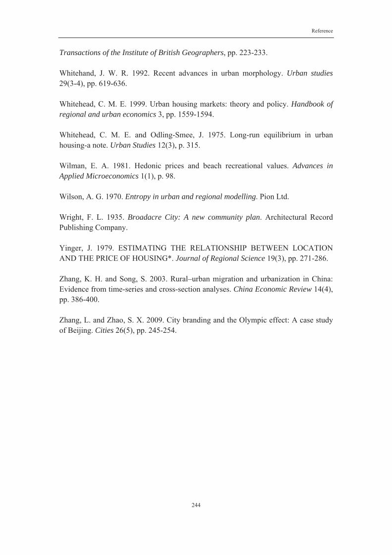
Reference

244

Transactions of the Institute of British Geographers, pp. 223-233. Whitehand, J. W. R. 1992. Recent advances in urban morphology. Urban studies 29(3-4), pp. 619-636. Whitehead, C. M. E. 1999. Urban housing markets: theory and policy. Handbook of regional and urban economics 3, pp. 1559-1594. Whitehead, C. M. E. and Odling-Smee, J. 1975. Long-run equilibrium in urban housing-a note. Urban Studies 12(3), p. 315. Wilman, E. A. 1981. Hedonic prices and beach recreational values. Advances in Applied Microeconomics 1(1), p. 98. Wilson, A. G. 1970. Entropy in urban and regional modelling. Pion Ltd. Wright, F. L. 1935. Broadacre City: A new community plan. Architectural Record Publishing Company. Yinger, J. 1979. ESTIMATING THE RELATIONSHIP BETWEEN LOCATION AND THE PRICE OF HOUSING*. Journal of Regional Science 19(3), pp. 271-286. Zhang, K. H. and Song, S. 2003. Rural–urban migration and urbanization in China: Evidence from time-series and cross-section analyses. China Economic Review 14(4), pp. 386-400. Zhang, L. and Zhao, S. X. 2009. City branding and the Olympic effect: A case study of Beijing. Cities 26(5), pp. 245-254.

245

Appendices

Appendix-4

246

Appendix-4

247

Appendix-4

248

Appendix-4

249

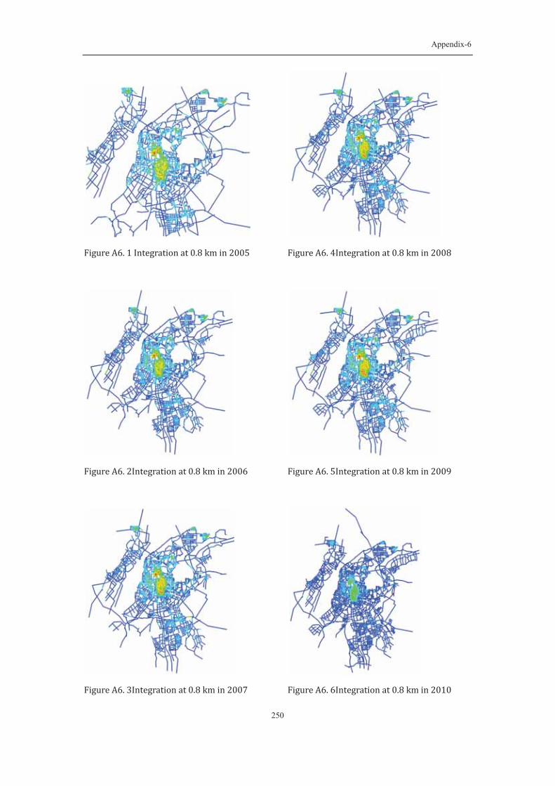
Appendix-6

250

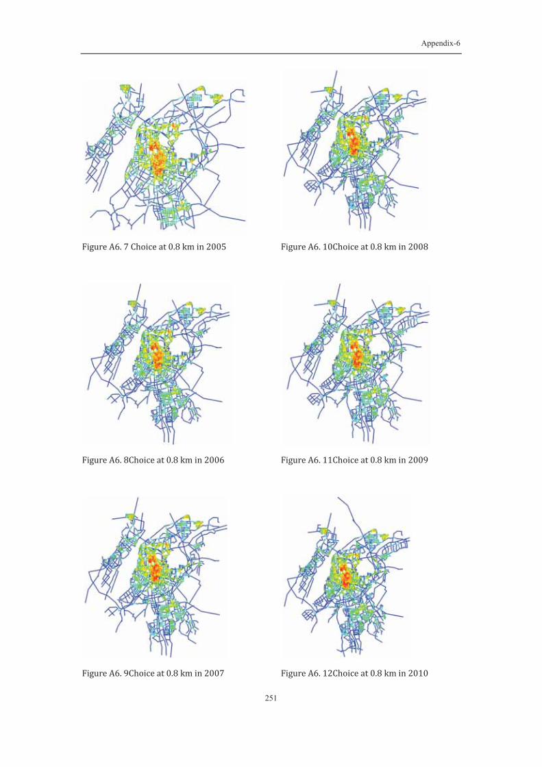
Appendix-6

251

Appendix-6

252

Appendix-6

253

Appendix-6

254

Appendix-6

255

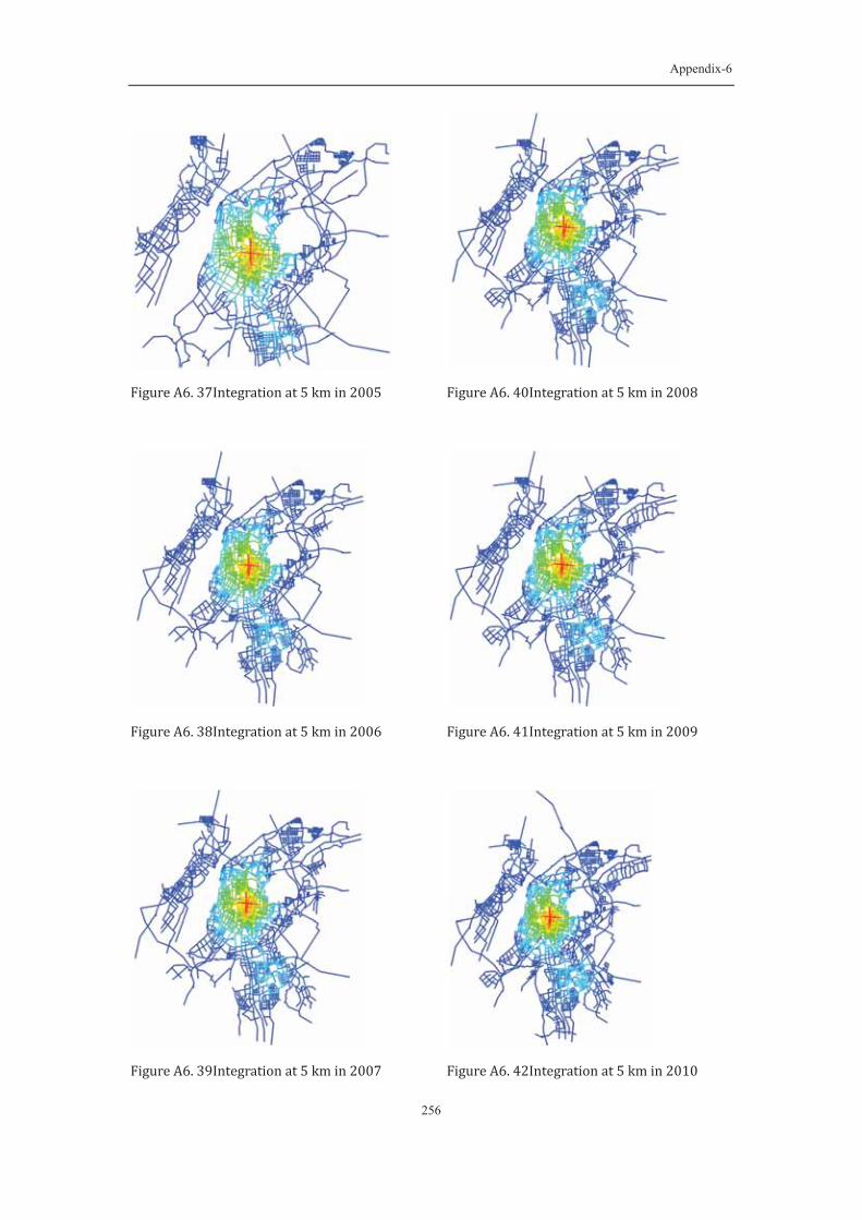
Appendix-6

256

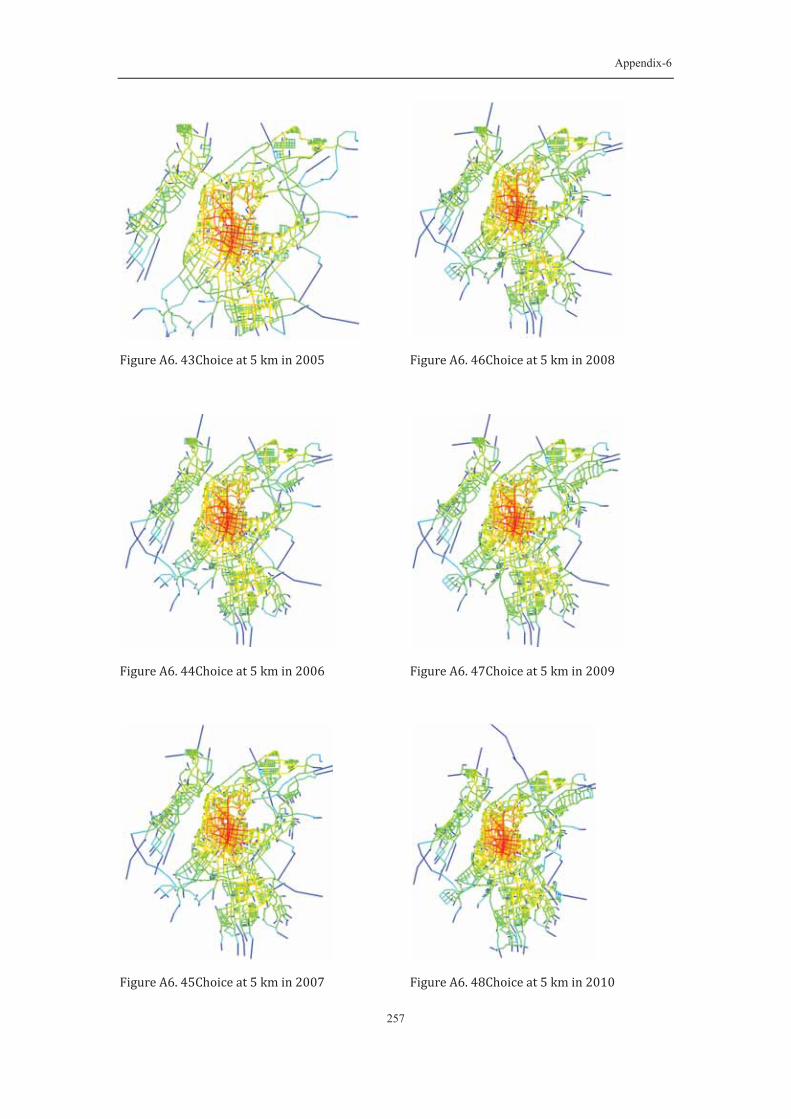
Appendix-6

257

Appendix-6

258

Appendix-6

259

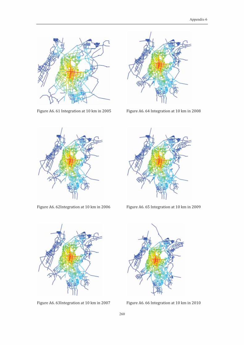
Appendix-6

260

Appendix-6

261

Appendix-6

262

Appendix-6

263

Appendix-6

264

Appendix-6

265

Appendix-6

266

Appendix-6

267

Appendix-6

268

Appendix-6

269

Urban Morphology and Housing Market - -ORCAorca.cf.ac.uk/44866/1/2013XiaoYphd.pdf · University of...

Documents

Transcript of Urban Morphology and Housing Market - -ORCAorca.cf.ac.uk/44866/1/2013XiaoYphd.pdf · University of...