URANS SIMULATIONS OF STATIC DRIFT AND DYNAMIC MANOUVERES OF THEKVLCC2 TANKER

S.R. Turnock(University of Southampton, Highfield, Southampton SO17 1BJ, UK)A.B. Phillips (University of Southampton, Highfield, Southampton SO17 1BJ, UK)

M. Furlong (National Oceanography Centre, Southampton, SO14 3ZH, UK)

1 SUMMARY

Computational Fluid Dynamics is used to investi-gate the global forces and moments acting on theKVLCC2 hull form under going straight line, driftand pure sway planar motion mechanism tests.Simulated results are compared with experimentalresults for the unappended hull in shallow waterand a fully appended hull with a propeller acting atthe ship self propulsion point. A body fitted meshundergoes transverse motion within an overall fixedmesh to capture planar motion mechanism tests.

A blade element momentum code is coupled with theRANS solver for the self propulsion case. A work-station is used for the calculations with mesh sizesup to 2x106 elements. Computational uncertainty istypically 2-3% for side force and yaw moment butgreater than 15% for resistance. With this meshmotion strategy manoeuvres can be well representedwithin a practical computational time scale.

2 INTRODUCTION

Traditionally the hydrodynamic derivatives for ves-sels are derived from a combination of towing tankexperiments, such as: yawed resistance tests, rotat-ing arm experiments and Planar Motion Mechanism(PMM) tests [1] or through the use of empirical for-mulas. This work investigates the quality of resultsthat can be achieved using a commercial ReynoldsAveraged Navier Stokes (RANS) flow solver, ANSYSCFX Version 11 [2]. This work is a contribution tothe SIMMAN workshop [3] and compares the resultsfrom CFD based methods with captive and freemodel tests performed by participating towing tanks.

The KRISO Very Large Crude Carrier 2 (KVLCC2),see Table 1, is hull the hullform considered.KVLCC2 was designed by the Korean Instituteof Ships and Ocean Engineering (KRISO) and isrepresentative of full boded ships such as tankers,see Figure 1.

Figure 1: KVLCC2 Hull Form

This investigation considers a combination of drift,pure sway PMM tests and self propulsion usingsteady and unsteady RANS simulations at varyingwater depths for direct comparison with experimen-tal results generated by INSEAN, [4] and MOERI

[5]. Model tests where performed on a 1/45.7 scalemodel of the hull form at Insean No. 2 basin (220 mlong x 9 m wide x 3.5 depth) and at the MOERI testtank (200m long x 16m wide x 7 deep) on a 1/58.0scale model.

Table 1: Principal Dimensions of VesselDimension Full-Scale INSEAN MOERIScale 1.00 45.714 58.000Lpp (m) 320.0 7.0000 5.5172Bwl (m) 58.0 1.2688 1.0000D (m) 30.0 0.6563 0.5172T (m) 20.8 0.4550 0.3586∇ (m3) 312622 3.2724 1.6023

The aim of this work is to investigate the trade-off be-tween computational cost and fluid dynamic fidelityrequired for unsteady ship manoeuvres.

3 BARE HULL DRIFT AND PMM TESTS INSHALLOW WATER

A series of simulations of drift and PMM testswhere analysed for non-dimensional water depths,1.2, 1.5, 3.0 and 8.3 (non-dimensional water depthis defined as h/Tm where Tm is mean draught andh is the water depth). The tests where performedat a Froude number of 0.064 corresponding to avessel speed of 7kn full scale and 0.533 m/s modelscale, equating to a model scale Reynolds numberof 3.7x106. Drift tests were performed at a seriesof incidence angles from 0◦ to 8◦. PMM tests wereperformed at a frequency of 0.06 s−1.

In order to replicate the sway motion produced inthe experimental PMM tests the KVLCC2 geometrymoves within the domain, deforming the mesh. CFXhas an inbuilt ’mesh morphing’ model which is usedto calculate the new node locations at each timestep, while maintaining mesh topology. The modelcalculates the displacement on each node using aspring analogy method.

Consequently if the mesh surrounding the vehicle isallowed to deform the elements around the vehicledeform. This can quickly lead to poor qualityelements if care is not taken. An alternative methodis to replicate the motion of the vessel with thefluid domain split into an inner and outer region.The outer domain remains fixed in space while theinner domain containing the hull moves laterally toreplicate the motion induced by a PMM. The meshin the inner sub domain remains locked in positionrelative to the lateral motion of the vessel. This

prevents deformation of the detailed mesh aroundthe vessel. The mesh in the outer region is coarserwith the inner domain accounting for 89% of thevolume and 98% of the elements. The outer mesh isdeformed due to the motion of the inner region.

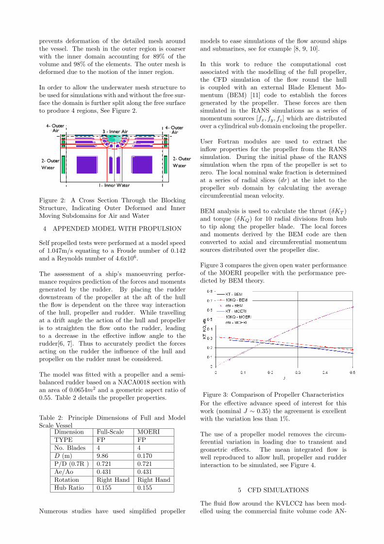
In order to allow the underwater mesh structure tobe used for simulations with and without the free sur-face the domain is further split along the free surfaceto produce 4 regions, See Figure 2.

Figure 2: A Cross Section Through the BlockingStructure, Indicating Outer Deformed and InnerMoving Subdomains for Air and Water

4 APPENDED MODEL WITH PROPULSION

Self propelled tests were performed at a model speedof 1.047m/s equating to a Froude number of 0.142and a Reynolds number of 4.6x106.

The assessment of a ship’s manoeuvring perfor-mance requires prediction of the forces and momentsgenerated by the rudder. By placing the rudderdownstream of the propeller at the aft of the hullthe flow is dependent on the three way interactionof the hull, propeller and rudder. While travellingat a drift angle the action of the hull and propelleris to straighten the flow onto the rudder, leadingto a decrease in the effective inflow angle to therudder[6, 7]. Thus to accurately predict the forcesacting on the rudder the influence of the hull andpropeller on the rudder must be considered.

The model was fitted with a propeller and a semi-balanced rudder based on a NACA0018 section withan area of 0.0654m2 and a geometric aspect ratio of0.55. Table 2 details the propeller properties.

Table 2: Principle Dimensions of Full and ModelScale Vessel

Dimension Full-Scale MOERITYPE FP FPNo. Blades 4 4D (m) 9.86 0.170P/D (0.7R ) 0.721 0.721Ae/Ao 0.431 0.431Rotation Right Hand Right HandHub Ratio 0.155 0.155

Numerous studies have used simplified propeller

models to ease simulations of the flow around shipsand submarines, see for example [8, 9, 10].

In this work to reduce the computational costassociated with the modelling of the full propeller,the CFD simulation of the flow round the hullis coupled with an external Blade Element Mo-mentum (BEM) [11] code to establish the forcesgenerated by the propeller. These forces are thensimulated in the RANS simulations as a series ofmomentum sources [fx, fy, fz] which are distributedover a cylindrical sub domain enclosing the propeller.

User Fortran modules are used to extract theinflow properties for the propeller from the RANSsimulation. During the initial phase of the RANSsimulation when the rpm of the propeller is set tozero. The local nominal wake fraction is determinedat a series of radial slices (dr) at the inlet to thepropeller sub domain by calculating the averagecircumferential mean velocity.

BEM analysis is used to calculate the thrust (δKT )and torque (δKQ) for 10 radial divisions from hubto tip along the propeller blade. The local forcesand moments derived by the BEM code are thenconverted to axial and circumferential momentumsources distributed over the propeller disc.

Figure 3 compares the given open water performanceof the MOERI propeller with the performance pre-dicted by BEM theory.

Figure 3: Comparison of Propeller CharacteristicsFor the effective advance speed of interest for thiswork (nominal J ∼ 0.35) the agreement is excellentwith the variation less than 1%.

The use of a propeller model removes the circum-ferential variation in loading due to transient andgeometric effects. The mean integrated flow iswell reproduced to allow hull, propeller and rudderinteraction to be simulated, see Figure 4.

5 CFD SIMULATIONS

The fluid flow around the KVLCC2 has been mod-elled using the commercial finite volume code AN-

Figure 4: Propeller Model

SYS CFX 11 (CFX) [2]. For these calculations thefluid’s motion is modelled using the incompressible(1), isothermal RANS equations (2) in order to de-termine the cartesian flow field (ui = u, v, w) andpressure (p) of the water around the hull:

∂Ui

∂x1= 0 (1)

∂Ui

∂t+

∂UiUj

∂xj

= −1

ρ

∂P

∂xi

+∂

∂xj

ν

„∂Ui

∂xj

+∂Uj

∂xi

«ff−

∂u′iu

′j

∂xj

+fi

(2)

In order to maximise the number of cases that couldbe considered most simulations have been performedassuming a flat free surface. For a few cases acoupled-implicit Volume of Fluid (VOF) algorithmis used to consider the influence of free surface [12].Details of the computational model are presented inTable 3.

Table 3: Computational modelParameter SettingTurbulence Model Shear Stress Transport [13]Multiphase Model Homogeneous Coupled VOFSpatial Discretisation High ResolutionTime Discretisation 2nd Order Backward EulerConvergence Control RMS residual < 10−5

5.1 Mesh Definition

Brogali et al. [14] used an in-house CFD code toinvestigate the blockage effects during PMM testsof the KVLCC2 in three different width modelbasins. The influence of tank walls on the calculatedderivatives was clearly identified, consequently forthese simulations the transverse domain size isselected to match the size of the tank.

For the bare hull configuration a structured mesh isrelatively easy to produce and allows rapid creationof multiple meshes. For the appended case creating asuitable blocking structure around the propeller andrudder becomes more complex and an unstructuredapproach has been used.

All meshes are produced in ANSYS ICEM version11 [15]. The meshes have been built with a firstelement thickness equating to a y+ ∼ 30, with 10 to15 elements in the boundary layer.

5.2 Boundary Conditions

To solve the RANS equations a series of boundaryconditions are defined. The hull is modelled usinga no-slip wall condition. A Dirichlet inlet condition,one body length upstream of the hull is defined wherethe inlet velocity and turbulence are prescribed ex-plicitly. The model scale velocity is replicated inthe CFD analyses; inlet turbulence is set at 5%. Amass flow outlet is positioned downstream of the hull.Three free slip wall conditions are placed at the loca-tions of the floor and sides of the appropriate tank,while the upper boundary is represented by a sym-metry plane on the free surface or an opening at decklevel if the free surface is considered.The length of thedomain was kept small to allow good aspect ratio el-ements on the free surface.

5.3 Running Simulations

Simulations were run on a high specificationdesktop pc running 64 bit Windows XP using anAMD Athalon 60 X2 Dual Core Processor 5000+(2.61GHZ) with 4 GB of RAM. The residual masserror was reduced by four orders of magnitude andlift and drag forces on the hull were monitored toensure convergence.

For the transient simulations initial steady state sim-ulations are performed to provide initial conditionsto the transient simulation. Transient motion simu-lations are then performed for 1.5 cycles. The firsthalf cycle allows the system to settle before measure-ment of the derivatives are made over a completecycle.

6 INDEPENDENCE STUDIES

6.1 Mesh Sensitivity

Two mesh sensitivity studies were performed, onefor each meshing strategy. The mesh sensitivitystudy is presented for the structured meshes for thedrift and PMM tests in shallow water at a driftangle of 0◦ and 6◦, see Table 4.

The variation in the global results between the fourmeshes is small (< 1.5%). This study is predomi-nantly interested in the prediction of sideforce andyaw moment to accurately derive hydrodynamicderivatives. These parameters can be derived with-out detailed flow information and so the mediummesh was selected for the shallow water cases.

Table 5 gives a mesh sensitivity is given for theself propelled case with the rudder at 10◦ using arefinement ratio of rk =

√2 with the finest mesh

having 2x106 elements. Uncertainty assessment hasbeen performed using the methodology presented byStern et al. [16].

Previous workshops [17, 18] highlight the difficultiesin accurate prediction of straight line resistance, with

Table 4: Mesh Sensitivity - Shallow Water Mesh h/Tm=8.3Drift Angle (deg) Mesh Nos Elements Run time (min) X (N) Y (N) N (Nm)

0 Coarse 359999 26 -8.101 0.0303 -0.0550 Medium 681170 48 -8.029 0.007 -0.0270 Fine 1325112 102 -7.984 0.009 -0.0220 Very Fine 1961000 150 -7.984 0.011 -0.0246 Coarse 359999 34 -9.451 10.900 48.6706 Medium 681170 48 -9.371 10.880 48.4606 Fine 1325112 108 -9.322 10.830 48.5726 Very Fine 1961000 168 -9.323 0.018 48.571

Table 5: Uncertainty Analysis - Self Propulsion Mesh Rudder at 10◦

Exp. (D) Fine (SG) Medium Coarse UG (%SG) E (%D) Uv (%D)Longitudinal Force, X (N) -11.05 -11.74 -12.60 -13.82 17.50 -6.28 18.77Transverse Force, Y (N) 6.79 7.60 7.51 7.33 1.35 -11.89 2.92Yaw Moment, N (Nm) -19.47 -18.75 -18.70 -18.35 0.49 3.70 2.54Thrust, T (N) 10.46 12.53 12.37 12.08 1.57 -19.79 3.13Rudder X Force, Rx (N) -2.02 -1.83 -1.89 -1.94 27.83 9.39 25.34Rudder Y Force, Ry (N) 4.32 4.94 4.99 4.88 1.23 -14.49 2.87

large uncertainty and comparison errors common be-tween calculated and experimental drag unless largermeshes (10M+ elements) are used. self propelledcases where only performed as steady state simula-tions, hence the finer mesh was used.

6.2 Time Step Sensitivity

Determining an appropriate time step for transientsimulations is necessary to ensure valid resultswhile minimising the total run time. There issignificant variation in the number of time stepsper oscillation used within the literature. Toinvestigate the effect simulations with 50, 100and 500 time steps per oscillation were performed,corresponding to a Courant number of 7, 3.5 and 0.7.

Results for the variation in sway force are illustratedin Figure 5. For all three cases instabilities are ob-served during the initial stages of the transient simu-lation, however, the variation of sway force and yawmoment have stabilised after less than quarter of anoscillation.

Figure 5: Variation in Predicted Sway Force withVarying Timesteps

7 RESULTS

The results are non-dimensionalised by the lengthof the vehicle (L) the velocity of the vehicle (V)and the density of the fluid (ρ), a prime symbol isused to signify the non dimensional form for example:

v′ =v

V, Y ′ =

Y

1/2ρL2V 2, N ′ =

N

1/2ρL3V 2(3)

The matching set of experiments were performedwith the vessel restrained in roll but free to heaveand pitch, however, to reduce simulation time theCFD simulations have assumed the vessel is fixed inheave and pitch at the quoted mean draught andlevel keel.

7.1 Bare Hull Drift and PMM Tests in Shallow Wa-ter

Results are presented for a medium mesh of 700,000elements. The Froude number (0.064)for the modeltests is small consequently unless stated the resultsdo not include free surface effects. The free surfacesimulations typically increase computational cost by1000% runtime to allow the wave pattern to develop.

When operating in shallow water the water velocityaround the ship is accelerated due to the restrictioncreated by the seabed, see Fig 6. This results inlarger forces and moments acting on the vessel.Figure 7 shows how the depth influences the flowpattern around the hull at a 6◦ drift angle, althoughthe meshes are not fine enough to completely resolvethe vortex structures. For the shallow water casethere are two distinct vortex structures formingaround the hull, one which separates from the bilgeat the forward shoulder on the pressure side andone which separates at the aft end of the bilge. Theforward vortex structure is not present in the deepwater case and the aft vortex remains attached until

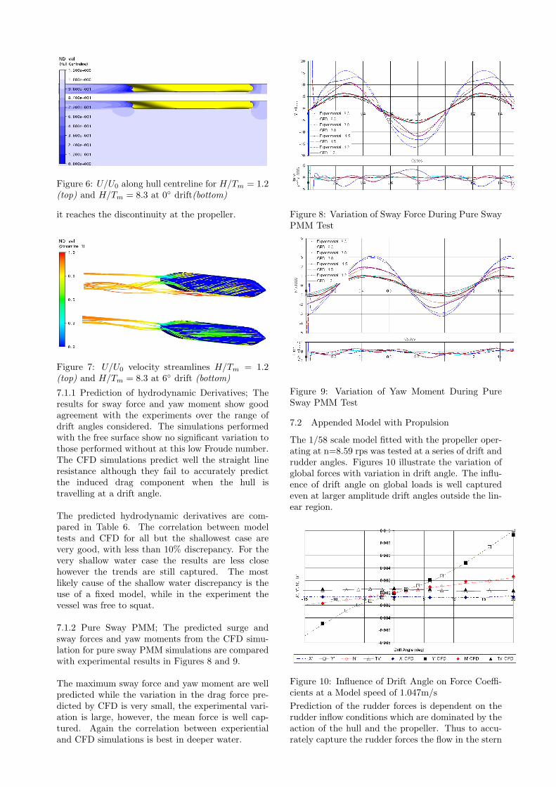
Figure 6: U/U0 along hull centreline for H/Tm = 1.2(top) and H/Tm = 8.3 at 0◦ drift(bottom)

it reaches the discontinuity at the propeller.

Figure 7: U/U0 velocity streamlines H/Tm = 1.2(top) and H/Tm = 8.3 at 6◦ drift (bottom)

7.1.1 Prediction of hydrodynamic Derivatives; Theresults for sway force and yaw moment show goodagreement with the experiments over the range ofdrift angles considered. The simulations performedwith the free surface show no significant variation tothose performed without at this low Froude number.The CFD simulations predict well the straight lineresistance although they fail to accurately predictthe induced drag component when the hull istravelling at a drift angle.

The predicted hydrodynamic derivatives are com-pared in Table 6. The correlation between modeltests and CFD for all but the shallowest case arevery good, with less than 10% discrepancy. For thevery shallow water case the results are less closehowever the trends are still captured. The mostlikely cause of the shallow water discrepancy is theuse of a fixed model, while in the experiment thevessel was free to squat.

7.1.2 Pure Sway PMM; The predicted surge andsway forces and yaw moments from the CFD simu-lation for pure sway PMM simulations are comparedwith experimental results in Figures 8 and 9.

The maximum sway force and yaw moment are wellpredicted while the variation in the drag force pre-dicted by CFD is very small, the experimental vari-ation is large, however, the mean force is well cap-tured. Again the correlation between experientialand CFD simulations is best in deeper water.

Figure 8: Variation of Sway Force During Pure SwayPMM Test

Figure 9: Variation of Yaw Moment During PureSway PMM Test

7.2 Appended Model with Propulsion

The 1/58 scale model fitted with the propeller oper-ating at n=8.59 rps was tested at a series of drift andrudder angles. Figures 10 illustrate the variation ofglobal forces with variation in drift angle. The influ-ence of drift angle on global loads is well capturedeven at larger amplitude drift angles outside the lin-ear region.

Figure 10: Influence of Drift Angle on Force Coeffi-cients at a Model speed of 1.047m/sPrediction of the rudder forces is dependent on therudder inflow conditions which are dominated by theaction of the hull and the propeller. Thus to accu-rately capture the rudder forces the flow in the stern

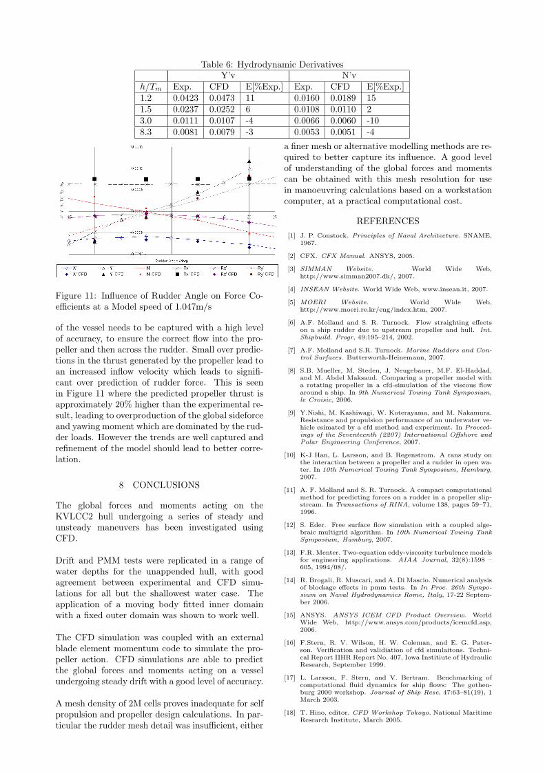
Table 6: Hydrodynamic DerivativesY’v N’v

h/Tm Exp. CFD E[%Exp.] Exp. CFD E[%Exp.]1.2 0.0423 0.0473 11 0.0160 0.0189 151.5 0.0237 0.0252 6 0.0108 0.0110 23.0 0.0111 0.0107 -4 0.0066 0.0060 -108.3 0.0081 0.0079 -3 0.0053 0.0051 -4

Figure 11: Influence of Rudder Angle on Force Co-efficients at a Model speed of 1.047m/s

of the vessel needs to be captured with a high levelof accuracy, to ensure the correct flow into the pro-peller and then across the rudder. Small over predic-tions in the thrust generated by the propeller lead toan increased inflow velocity which leads to signifi-cant over prediction of rudder force. This is seenin Figure 11 where the predicted propeller thrust isapproximately 20% higher than the experimental re-sult, leading to overproduction of the global sideforceand yawing moment which are dominated by the rud-der loads. However the trends are well captured andrefinement of the model should lead to better corre-lation.

8 CONCLUSIONS

The global forces and moments acting on theKVLCC2 hull undergoing a series of steady andunsteady maneuvers has been investigated usingCFD.

Drift and PMM tests were replicated in a range ofwater depths for the unappended hull, with goodagreement between experimental and CFD simu-lations for all but the shallowest water case. Theapplication of a moving body fitted inner domainwith a fixed outer domain was shown to work well.

The CFD simulation was coupled with an externalblade element momentum code to simulate the pro-peller action. CFD simulations are able to predictthe global forces and moments acting on a vesselundergoing steady drift with a good level of accuracy.

A mesh density of 2M cells proves inadequate for selfpropulsion and propeller design calculations. In par-ticular the rudder mesh detail was insufficient, either

a finer mesh or alternative modelling methods are re-quired to better capture its influence. A good levelof understanding of the global forces and momentscan be obtained with this mesh resolution for usein manoeuvring calculations based on a workstationcomputer, at a practical computational cost.

REFERENCES[1] J. P. Constock. Principles of Naval Architecture. SNAME,

1967.

[2] CFX. CFX Manual. ANSYS, 2005.

[3] SIMMAN Website. World Wide Web,http://www.simman2007.dk/, 2007.

[4] INSEAN Website. World Wide Web, www.insean.it, 2007.

[5] MOERI Website. World Wide Web,http://www.moeri.re.kr/eng/index.htm, 2007.

[6] A.F. Molland and S. R. Turnock. Flow straighting effectson a ship rudder due to upstream propeller and hull. Int.Shipbuild. Progr, 49:195–214, 2002.

[7] A.F. Molland and S.R. Turnock. Marine Rudders and Con-trol Surfaces. Butterworth-Heinemann, 2007.

[8] S.B. Mueller, M. Steden, J. Neugebauer, M.F. El-Haddad,and M. Abdel Maksaud. Comparing a propeller model witha rotating propeller in a cfd-simulation of the viscous flowaround a ship. In 9th Numerical Towing Tank Symposium,le Croisic, 2006.

[9] Y.Nishi, M. Kashiwagi, W. Koterayama, and M. Nakamura.Resistance and propulsion performance of an underwater ve-hicle esimated by a cfd method and experiment. In Proceed-ings of the Seventeenth (2207) International Offshore andPolar Engineering Conference, 2007.

[10] K-J Han, L. Larsson, and B. Regenstrom. A rans study onthe interaction between a propeller and a rudder in open wa-ter. In 10th Numerical Towing Tank Symposium, Hamburg,2007.

[11] A. F. Molland and S. R. Turnock. A compact computationalmethod for predicting forces on a rudder in a propeller slip-stream. In Transactions of RINA, volume 138, pages 59–71,1996.

[12] S. Eder. Free surface flow simulation with a coupled alge-braic multigrid algorithm. In 10th Numerical Towing TankSymposium, Hamburg, 2007.

[13] F.R. Menter. Two-equation eddy-viscosity turbulence modelsfor engineering applications. AIAA Journal, 32(8):1598 –605, 1994/08/.

[14] R. Brogali, R. Muscari, and A. Di Mascio. Numerical analysisof blockage effects in pmm tests. In In Proc. 26th Sympo-sium on Naval Hydrodynamics Rome, Italy, 17-22 Septem-ber 2006.

[15] ANSYS. ANSYS ICEM CFD Product Overview. WorldWide Web, http://www.ansys.com/products/icemcfd.asp,2006.

[16] F.Stern, R. V. Wilson, H. W. Coleman, and E. G. Pater-son. Verification and validiation of cfd simulaitons. Techni-cal Report IIHR Report No. 407, Iowa Institiute of HydraulicResearch, September 1999.

[17] L. Larsson, F. Stern, and V. Bertram. Benchmarking ofcomputational fluid dynamics for ship flows: The gothen-burg 2000 workshop. Journal of Ship Rese, 47:63–81(19), 1March 2003.

[18] T. Hino, editor. CFD Workshop Tokoyo. National MaritimeResearch Institute, March 2005.