Upsampling Fluid Simulations

Felix Konig∗

TU ViennaInstitute of Computer Graphics and Algorithms

Abstract

This paper aims at presenting fluid simulations on an Eulerian gridand explores different strategies which improve those simulations.The first section elaborates on the building blocks for advanced al-gorithms. The fundamental concepts of a standard fluid solver arecovered in great detail. The paper therefore also serves as an intro-ductory reading to people that are not familiar with the basic con-cepts of Navier-Stokes equations and grid like numerical solvers.All advanced methods are described in the following chapters. Fur-thermore, the paper also discusses hybrid approaches between La-grangian and purely Eulerian methods. The conclusion gives anoutline and comparison of the presented techniques.

CR Categories: 1.3.7 [Computer Graphics]: Three-DimensionalGraphics and Realism—Animation;1.3.5 [Computer Graphics]:Computational Geometry and Object Modeling— Physically basedmodeling

Keywords: fluid simulation, Navier-Stokes equations, tetrahe-dral discretization, adaptivity, wavelet turbulence, vorticity confine-ment, Lagrangian fluid simulation, procedural noise, extrapolation,PDE solvers, stable solvers

1 Introduction

The topic of simulating both visually convincing and physically re-alistic dynamics of fluids and smoke is important in the field of an-imation, cinematography and within the development of computergames. The creation of new algorithms that model complex mo-tion of fluids depends on different factors. Computations should ofcourse be as fast as possible and their results are expected to delivera level of detail and complexity that is comparable to real naturephenomena. At the same time, algorithms ought to provide enough

∗e-mail: e0917104@student.tuwien.ac.at

flexibility for the artist to deviate from pure physical realism butstill achieve convincing animations. Recent algorithms can be di-vided into two classes while both classes try to add more detail intoa simulation:

• Algorithms that try to improve the numerical approximationsthat a fluid solver makes and

• algorithms that try to provide a convincing feel of realism.

All of those classes try to achieve their results with as minimal com-putational overhead as possible. Especially if those algorithms arenot entirely physically accurate, details are synthesized in a fashionthat allows fast computation of results.

2 Basic concepts of fluid dynamics

This section covers the basics of systems that model fluid motionand is meant as an introduction in order to understand more sophis-ticated approaches.

2.1 The Navier-Stokes equations

The core component of a system that models fluid mechanics arethe Navier-Stokes equations:

∂u∂ t

=−(u ·∇)u︸ ︷︷ ︸advection

− 1ρ

∇p︸ ︷︷ ︸pressure

+ ν∇2u︸ ︷︷ ︸

di f f usion

+ Fext︸︷︷︸external f orces

, (1)

∇ ·u = 0, (2)

where u denotes the velocity field, p stands for the pressure field,ν describes the material viscosity, ρ is the density and Fext is theexternal force field. The left hand side of equation 1 depicts thetemporal change of the velocity field and is called momentumequation. The Navier-Stokes system essentially describes how themotion of a particle in a fluid is continued. The meaning of theaforementioned symbols is kept consistent throughout the wholepaper. Equation 2 is called the incompressibility constraint andnecessary for providing stable solvers.

The momentum equation consists of four major terms thatcan be described intuitively.

Advection: The term advection refers to the inherent prop-erty of a fluid which makes objects inside it follow a certain flow.However the equation also describes the movement of the velocityfield by itself which is modeled by the term (u ·∇). As a result, notonly objects are moved by the velocity field, it moves or advectsitself. This is also the reason why solving fluid dynamics is hard. Itis still not clear if there always exists an analytic smooth solutionto these equations. This is called the Navier–Stokes existenceand smoothness problem which is part of the Millennium PrizeProblems. Figure 1 depicts the advection of smoke densities. In

Figure 1: The advection moving a set of smoke particles along astatic velocity field [Stam 2003].

this image, the velocities are not advected.

Pressure: Pressure forces that are exerted on each fluid aremodeled by this term. The gradient of the pressure field ∇ppoints towards the steepest ascend of the field. However, due tothe laws of physics, the particle is pushed from a higher pressureregion to a lower one which is denoted by the minus sign. Sincedenser particles are harder to accelerate, the force is divided by theparticles density ρ . An example for this behavior can be describedby smoke particles that dissolve faster than thick liquid substancessuch as honey due to the lower amount of density present withinsmoke.

Diffusion: Different concentrations inside a fluid tend to av-erage themselves out in order to achieve an equilibrium state.Dropping a viscous substance into a fluid results into diffusion.Depending on the viscosity, the diffusion proceeds more rapidly orslowly. This is the reason for the appearance of ν in the equation.The Laplace Operator ∇2 models the diffusion in a sense that ithas a high value if the average difference of the neighboring valuesof u is high. If the adjoint velocities differ to a smaller extent, thediffusion force is weaker. Therefore the optimal equilibrium stateis reached if ∇2u = 0.

External force field: The external force field allows to addadditional forces which can model heat, user interaction, windor user defined constraints such as shaping the fluid motion in aparticular fashion that is suitable for the artists intentions. Forexample, an artist could define a target pressure model to whichthe fluid should converge. An illustration of such a user definedshaping can be seen in Figure 2. In some circumstances [Fedkiwet al. 2001] a smoke simulator can be defined that employs atemperature model that further alters the experienced velocity. Theforce term is called buoyancy and evaluates as follows:

Fbuoy =(−αρ +β (T −Tamb)

)z. (3)

In this case, z points in the vertical direction and Tamb is the tem-perature of the air. Furthermore, α > 0 and β > 0 are physicallymeaningful constants and T is the temperature of smoke. The firstterm −αρ is a gravitational force which pulls heavier particlestowards the ground. The second term β (T −Tamb) is positive when

Figure 2: Shaping fluids into a structure by using external forcefields. The image was taken from the 2012 reel video of Fusion CIStudios.

T > Tamb and acts as an uplifting force, otherwise it accelerates thegravitational pull.

In addition to equations 1 and 2, the movement of the den-sity field ρ is often incorporated into fluid systems [Stam 2003].The equation has a similar notion as the momentum equation:

∂ρ

∂ t=−(u ·∇)ρ +κ∇

2ρ +S. (4)

The intention is to model the advection of the densities that iscaused by the first term on the right hand side of equation 4. Thediffusion is denoted by the second term and the term S correspondsto the addition of an external force specific to the density field ρ .Similar to the viscosity constant ν , κ denotes the strength of thedensities to which extent they do withstand diffusion. The sameprinciple of the momentum equation can also be applied to otherscalar fields besides ρ such as the temperature T for instance.

The incompressibility condition states that the fluid con-serves mass and can be understood intuitively. As we integratethe influx and efflux of a fluid over an arbitrarily shaped, closedsurface with boundary ∂Ω, the result should always yield zero.This is due to the fact that no density is lost inside the volume.Mathematically speaking, the equation is written as follows:∫ ∫

∂Ω

u ·n dΩ =∫ ∫ ∫

Ω

u ·∇ dΩ = 0, (5)

where n denotes the normal along the boundary ∂Ω. In order toresolve to 0, the integrand u ·∇ must be 0 and this yields the incom-pressibility condition. A vector field u that fulfills this condition isalso called divergence free [Stam 1999].

2.2 Enforcing the Incompressibility Condition

Upon solving equation 1 of the Navier-Stokes system, it needs to beensured that the resulting vector field u is divergence free. Since asolver operates on time based iterations where each iteration coversa time interval ∆t, this constraint needs to be enforced after eachtime step. This step is usually performed by solving a Poissonequation [Ando et al. 2013] or via the Helmholtz-Hodge Decom-position [Stam 1999]. The latter states that any vector field w canbe decomposed into:

w = u+∇q, (6)

where u is divergence free and q is a scalar field. Therefore, u canbe made divergence free by applying the projection P:

u = P(w) = w−∇q. (7)

In terms of the first Navier-Stokes equation this means that we needto solve:

∂u∂ t

= P(− (u ·∇)u+ν∇

2u+Fext), (8)

where the term P(∇p)

vanishes due to Equation 7 and because of

the linearity of P. Furthermore, P(

∂u∂ t

)= ∂u

∂ t as P(u) = u becauseof the divergence free property of u and the same holds for the par-tial derivative as long as u is smooth.As mentioned before, the second option to extract the divergencefree part of any vector field is accomplished by solving a Poissonequation. If we multiply both sides in Equation 6 with ∇, we endup with:

∇w = ∇2q, (9)

as ∇ · v = 0. This is precisely the Poisson equation. As Navier-Stokes equations are solved over discrete time steps this equationturns into:

∆t∇2q = ∇w (10)

In order to extract the divergence free part, we need to compute theminimal amount of energy that is necessary to change the state intoan incompressible one. This can be achieved via energy minimiza-tion:

q = argminq

∫Ω

12‖w−∆t∇q‖2dΩ. (11)

2.3 Vorticity Confinement

Another important property of fluids is the concept of vorticity con-finement. This aspect of fluids is not directly composed inside theNavier-Stokes equations but still corresponds to a component ofevery fluid motion. It becomes particularly important if the fluidsolver is executed on a coarse grid which means that some amountof high frequency details cannot be properly computed. One wayto add such lost energy into the system is by using the concept ofvorticity confinement [Fedkiw et al. 2001]. This effect becomes ap-parent when fluids of low viscosity are rapidly accelerated by thevelocity u. The flow might follow a turbulent pattern which can alsobe observed when the fluid is pushed around an obstacle as depictedin Figure 3. The vorticity of a vector field can be described by:

Figure 3: Smoke particles that are pushed around a ball where highvorticity can be observed [Fedkiw et al. 2001].

ω = ∇×u, (12)

which holds for incompressible flows. After obtaining the vorticity,a force can be defined that is directed towards the center of thecorresponding vortex:

µ = ∇|ω|. (13)

The resulting force field is depicted in Figure 4. As µ conveys not

Figure 4: Visualization of the force field µ [Fedkiw et al. 2001].

only the direction, but also the size of the vortex, this term is nor-malized by a division through |µ| and called N. The reason is thatthe strength of the rotation in the vortex should be adjusted manu-ally. The rotation is obtained by taking the cross product betweenN and ω multiplied by a weighting term ε:

Fcon f = εh(N×ω). (14)

In Equation 14 the parameter h corresponds to the amount of spa-tial discretization. The higher the discretization factor is, the fastersmall scale details such as vorticity will be damped out. Thereforethe added force ε(N×ω) should be scaled appropriately.

2.4 Solving the Navier-Stokes on a Finite EulerianGrid

A numerical solution to the Navier-Stokes equations is composedof the following steps that are described in [Fedkiw et al. 2001].Initially, scalar, pressure and density fields are stored in memorytogether with a predefined force field Fext or a model to obtain suchexternal forces. A velocity field may or may not be present as it canevolve over time. The next steps require:

1. Computing and adding external forces Fext ,

2. advecting the velocity field,

3. computing the diffusion and

4. applying the projection operator P described in equation 8.

The evaluation of these steps is usually performed on a 2 or 3 di-mensional grid where finite differentials of the Nabla and Laplaceoperators can be used instead of continuous derivatives. Further-more, those iterations are performed for a finite time interval ∆t asmentioned in section 2.2. The coarseness of the grid in both spaceand time determines the numerical error of the method which is alsodependent on the order of the solver that is used. Using a densegrid requires more time demanding computations but at the sametime the accuracy of the solution is improved. Advanced methodsdescribed in further sections deal with this trade-off. A key com-ponent of the computation involves the evaluation of the advectionterm which should not be solved via a forward projection. The ve-locity vectors in these grids can reside at the center of each grid

cell or at the faces of each cell, depending on the used algorithm,different strategies are employed.Supposing that the initial state of u is u(x, t), where x is the positionof the grid cell and t is the current time, we can evaluate the systemas follows. The partial solution u1(x, t+∆t) is obtained after addingthe forces:

u1(x, t +∆t) = u(x, t)+∆tFext , (15)

where the assumption has been made that the forces do not varysignificantly during ∆t.Concerning the advection, a system of finite differences could bedescribed and solved, also denoted as forward projection. Thismethod however, is not stable in a sense that the velocity valueswill quickly blow up and diverge if the time step ∆t is not suffi-ciently small. Dealing with small time steps is also infeasible be-cause of the computational effort. The key idea of a stable solutioncan be understood intuitively and is presented in [Stam 1999] aswell as [Stam 2003]. Instead of forward projecting velocities, a

(a) Particle (b) Tracing (c) Gridvelocities

(d) Interpola-tion

Figure 5: Tracing the velocities back in time [Stam 2003].

backtracing step is introduced. In the previously obtained veloc-ity field u1(x, t +∆t), the point x should have been advected fromt to t +∆t. Therefore this point is traced backwards along the pathp(x,s) on which it traveled from the previous time step to the cur-rent one. Its velocity is then changed to the velocity of the previoustime step at the location p(x,−∆t). The newly acquired force isthen:

u2(x, t +∆t) = u1(

p(x,−∆t), t +∆t)

(16)

At this point it is important to consider that the point p(x,−∆t)must not lie on the center of a grid cell, actually, this is rarelythe case. Therefore, its true velocity value must be obtained byinterpolating the velocities on the neighboring grid cells or faces,depending on where the velocities are stored. Figure 5 illustratesthe backtrace step along with the interpolation, in this case, thevelocities are stored at the grid cells faces. In subfigure 5a, thevelocity u1(x, t +∆t) is shown, backtracing is depicted in subfig-ure 5b. The neighboring velocities of the point at p(x,−∆t) areshown in subfigure 5c. The final velocity is then interpolated withbilinear interpolation as the calculations are performed on a 2 di-mensional grid. The interpolation can be changed to a cubic ortrilinear model if more accuracy is needed or the grid size is 3 di-mensional. This method of calculating the advection is also knownas the semi-Lagrangian scheme.As a next step, the diffusion needs to be computed that is equivalentto the standard wave equation:

∂u2

∂ t= ν∇

2u2. (17)

A solution to this equation can be computed by solving a dis-cretized version of ∇2.

Level-set functions: As explained in Section 2.1 any phys-ical quantity such as densities, temperatures or velocities can beadvected by u. In case of an Eulerian grid, it would be insufficientto model the whole n dimensional space because only a portion of

all cells contain fluids. Therefore, a level set function ϕ(x, t) isused to describe the subset of grid cells that contain the fluid. It isan implicit surface function where (x, t) : ϕ(x, t) = 0 describesthe boundary of the fluid. The signed distance of ϕ(x, t) is storedon each grid cell x and is either positive when it is outside of theliquid or negative when it lies inside of the liquid. The evolution ofa liquid in space and time is described by:

∂ϕ

∂ t=−u ·∇ϕ. (18)

3 Frequency-Based Upsampling

When working on improvements of the numerical dissipation pro-duced by finite and coarsely spaced simulation grids, informationabout the frequency spectrum that fluids convey can help in pro-ducing a more realistic output. This section explains how frequencyanalysis can be used in the fluid simulation. The goal is to gener-ate artificial noise patterns and add them to the existing fluid in arealistic way using spectral components. The requirement of a real-istic noise function is that it should contain high frequency detailsthat are not present in the system. Furthermore, the noise should beadded only at the positions where such information is lost.

3.1 Wavelet Noise and Wavelet Theory

A highly valuable tool in examining frequency information of inputsignals is the Fourier-Transform. This transformation preciselyextracts the frequency components of a input function. However,one can not distinguish at which point in time certain frequenciesexist in the signal. This is due to the Gabor limit which states thatit is not possible to determine a functions power spectrum for boththe frequency and time information with arbitrary fineness [Cohen1995]. In case of the Fourier-transform, precise localizationof the frequency is possible by completely sacrificing the timelocalization. In contrast, the wavelet transform allows time andfrequency analysis in conjunction, however, the Gabor limit is stillpresent. This is reflected by the fact that precise frequency analysisof lower frequency components is possible but the time localizationis poor and vice versa for high frequency components.Wavelet functions are important when well constrained noisepatterns need to be constructed. The first approach in designingsuch procedural textures at different frequency levels was madein [Perlin and Velho 1995]. The authors explain how artificialdetails in a texture can be added to an image and its magnified andreduced versions. If an image is modified at the resolution 2n×2n

and later changed to a resolution of 2n−1 × 2n−1 it needs to beblurred before this change can be applied. The blurring is nec-essary, otherwise the picture at the new resolution would containaliasing artifacts because of the high frequency components thatcannot be properly displayed at a lower resolution. Filtering theimage with a Gauss kernel is the typical approach when removalof such problematic high frequency components is desired. If thepicture is again upsampled to 2n× 2n these lost details need to beadded back and this is done by storing them in a separate 2n× 2n

matrix. A bandpass pyramid can be created that contains thelost frequencies up to scale 21× 21. [Perlin and Velho 1995] alsodescribes that noise can be added and removed beyond the initialmaximum resolution of an image. This resolution corresponds tothe Nyquist limit. The method however, is not entirely aliasingfree as discussed in [Cook and DeRose 2005]. Therefore, theauthors of this work introduced a noise generation method thatproduces no aliasing artifacts even when noise patterns are createdbeyond the Nyquist limit. This is especially important if upsampled

fluid movements need to be created that lie above the resolutionof the finite grid cells, e.g. above the Nyquist limit of the simulation.

The authors of [Cook and DeRose 2005] proved that thereexists a noise function N(x) that can be upsampled and downsam-pled without creating additional aliasing artifacts, even if the noiseis above the Nyquist limit of the image:∫

N(2 jx− l)K(x− i)dx = 0. (19)

The above equation describes the downsampling of random noiseN generated at resolution j ≥ 0 while the image has a resolutionof j = −1. K(x− i) is the smoothing kernel that is applied. Equa-tion 19 evaluates to zero because the noise in higher resolutions isorthogonal to the filter kernel. Thus N(x) has no effect on imageswith a lower resolution.Suppose a basis function φ(x) was given at an arbitrary resolutionwhich is called 0. We can build other functions from φ by usinglinear combinations of the input:

F(x) = ∑i

fiφ(x− i). (20)

The set of all such functions with varying fi is called the vectorspace S0.Concerning noise patterns, it is important that noise ona higher resolution enriches the space S0 such that S0 ⊂ S1. Thisbehavior can be enforced by choosing refinable basis functions φ

such as B-splines. If this criterion is not satisfied, noise patternswould inconsistently change during subsequent upsampling steps,resulting in visual artifacts.Furthermore, all functions G(x) ∈ S1 must be representable in S0

without generating aliasing artifacts. This can be achieved by:

G(x) = G↓(x)+D(x), (21)

where G↓(x) is the approximation of G(x) that lies in S0 obtainedwith least squares error minimization. D(x) contains the part ofG(x) that is unrepresentable in S0. In order to prevent aliasing,D(x) must be orthogonal to all functions in S0. The vector spaceof all functions D(x) that satisfy this constraint is called the waveletspace W 0. If the noise function resides in the aforementioned vectorspace, it won’t affect images on lower resolutions.Using this knowledge, noise patterns can be created as follows:

1. Generate random coefficients R = (. . . ,ri, . . .).

2. Use B-spline basis functions B(x) to create R(x) ∈ S1.

3. R(x) = ∑i riB(2x− i).

4. Compute the least squares approximation R↓(x).

5. Decompose R(x) = R↓(x)+N(x) as shown in equation 21.

6. Extract N(x) = ∑i niB(2x− i).

3.2 Wavelet turbulence

The authors of [Kim et al. 2008] propose an upsampling techniquefor fluid systems that relies on the results explained in section3.1. The core idea of the paper is to solve the Navier-Stokes on acoarse grid and subsequently add details to the simulation wherethey are lost. Furthermore, temporal coherence of the newly addedfrequencies is preserved and the results are synthesized into a gridof refined size. This allows an artist to precompute the Navier-Stokes and add fine details later during post-processing when theyare needed. Since wavelets are used, high frequency details do

not interfere with the low frequency components produced by thesolver.

The wavelet noise function N(x) is adjusted to model tur-

Figure 6: Wavelet noise N(x) on the left is used to create a turbulentflow on the right w(x) = ∇×N(x) [Kim et al. 2008].

bulent flows as depicted in Figure 6. The model is similar to thevorticity that was determined form the velocity u, however it canalso be computed from the noise pattern itself leading to:

w(x) =(

∂N1

∂y− ∂N2

∂ z,

∂N3

∂ z− ∂N1

∂x,

∂N2

∂x− ∂N3

∂y

). (22)

It should be noted that N(x) is designed as a scalar function, so theauthors let N1, N2 and N3 correspond to one single noise functionwith an offset for each N∗. Taking partial derivatives from thenoise function does not destroy its band-limited properties as thederivative of a function in the frequency domain is linear. Thepartial derivatives are obtained by differentiating the weights ofthe B-spline function B(x). Furthermore, the resulting field w(x)retains its incompressibility.

A central concept is the property of forward scattering andbackward scattering inherent to fluids. Whenever fluids are inmotion, they generate large and small swirls that are denoted aseddies. When larger eddies move through the velocity field, someamount of compression and distortion leads to a break up intosmaller eddies. This type of movement is called forward scatteringand shown in Figure 7. Similarly, smaller eddies can be fused

Figure 7

together yielding the backward scattering effect. It is desirableto detect such behavior and incorporate those fine scale effectswhen they would happen on a small grid simulation. This can beachieved with Kolmogorov’s results in fluid analysis. A velocityfield always conveys kinetic energy in each grid cell x:

e(x) =12|u(x)|2. (23)

Kolmogorov’s analysis extracts the frequency components of thetotal energy et of the system at time t. The term et corresponds tothe summation of every grid cells energy. As stated previously insection 3.1 the wavelet transform allows the retrieval of frequencyand time information and is thus computed for various scales k on

the input function et . The result is Kolmogorov’s five-thirds powerlaw:

et(k) =Cε23 k−

53 , (24)

which states that within fine scale details, a decrease in kinetic en-ergy following a slope of − 5

3 steepness can be observed. Equa-tion 24 can be computed recursively:

et(2k) = et(k)2−53 ,et(1) =Cε

23 . (25)

Furthermore, 23 can be combined with 25 to create another recur-sion:

|u(x,2k))|= |u(x,k)|2−56 , |u(x,1))|= 2

12 C

12 ε

26 , (26)

where |u(x,k)| is the spectral component of u constructed on thefrequency band k. The final wavelet turbulence function can thenbe constructed:

y(x) =imax

∑i=imin

w(2ix)2−56 (i−imin). (27)

The deviation of equation 26 would suggest that we use |u(x,2i)|instead of w(2ix), however since we do not have the high frequencyinformation of u at certain bands above the Nyquist limit the noisefunction w that generates the additional detail must be substitutedaccordingly. In equation 27, imin and imax are used to constrain thenoise creation for a certain range of frequency bands.

Grid Expansion: As the simulation runs on coarse grid n3,but the turbulence is computed for a fine grid N3 where N3 > n3, anappropriate injection step needs to be defined. Simply interpolatingthe coarse grid would result in a smoothed out version of the inputvelocities and does not generate new turbulence, therefore theauthors suggest a model that computes the energy of the smallesteddie et

( n2)

and weights the turbulence function with this term.Additionally, turbulent eddies should only be added when forwardscattering occurs, therefore the authors make use of the energyspectrum in et

( n2)

to detect such a process. If the high resolutiongrid N3 is constructed, the density field can be advected on it.Except for the turbulence addition and successive advection, thecomputations are performed on the low resolution grid introducingonly minor overhead into the simulation while achieving drasticvisual improvements. In addition, the algorithm can be parallelizedbecause the individual steps of the extrapolation and turbulencecreation rely on local information on the grid. The authors useOpenMP to speed up the simulation and report a performanceimprove of 3.7 compared to a single core execution. Furthermore,the technique is independent of the underlying numerical solver.

Results of Wavelet Turbulence:

4 Higher order advection solvers

Another possibility of improving visual results of the Navier-Stokessolver is to refine the underlying numerical method. Whereas in theprevious section, artificial detail was added in a physically realisticfashion, the presented algorithms in this section deal with the nu-merical error that is produced by the finite resolution of an Euleriangrid. The key is to estimate the error of the advection step and cor-rect it. The methods in this section do not only improve the flowlocally as for example vorticity confinement, they also improve iton a macroscopic level since the overall motion is improved due toa smaller numerical error in the advection step.

Figure 8: Comparison of the simulation on the low resolution grid503 (left), and the high resolution synthesis on a 4003 grid (right)[Kim et al. 2008].

Figure 9: A wavelet turbulence simulation of smoke performed ona 50×100×50 coarse grid, eight frequency bands where used andsynthesized into a 12800× 25600× 12800 grid. The simulationachieved a framerate of 170s on 8 cores [Kim et al. 2008].

4.1 BFECC

BFECC is a shorthand notation for a technique called the Back andForth Error Correction and Compensation [Dupont and Liu 2003].It is applied to the level set function and compensates the error inthe semi-Lagrangian advection step. The algorithm is composed ofthe following steps:

1. Solve equation 18 using the semi-Lagrangian method and ob-tain ϕ(x, t +∆t).

2. Solve equation 18 backward in time and denote the result asϕ(x, t).

3. Compute the error e that is introduced by the forward andbackward steps: ϕ(x, t) = ϕ(x, t) + 2e, e = − 1

2 (ϕ(x, t)−ϕ(x, t)).

4. Solve equation 18 again with ϕ(x, t) = ϕ(x, t)− e being theinitial value.

The key is to incorporate the error e that is introduced by the La-grangian method and compensate it by subtraction in the last step.The BFECC method can be applied to the advection of velocities,densities and level sets as described in [B. Kim 2005]. The paperoutlines that, upon employing velocity advection with the BFECCmethod, physically realistic small scale fluctuations around obsta-cles on coarse Eulerian grids can be achieved. Furthermore, rigidbody motion of objects in a fluid can be computed more accurate.This was shown by dropping a cup into water. The object sinksimmediately into the water when the standard advection method is

applied, whereas the BFECC advection causes the cup to tumblecorrectly and subsequently it sinks to the ground. The price to payis the additional invocation of a semi-Lagrangian solver, howeverthe method is still computationally cheaper than refining the grid.In fact, the advection has a computational cost of Θ(n3) and in-creases exponentially with n, whereas the increase in complexitywith BFECC is linear: Θ(3n3).

4.2 MacCormack Method

The MacCormack method which is described in [Selle et al. 2008],further reduces the computational complexity of the BFECC algo-rithm. Step 4 in the latter algorithm can be described by A(ϕ(x, t)−e), where A denotes the semi-Lagrangian advection step. As A islinear and e is not a quantity that needs to be advected since it doesnot convey any information of ϕ , the formula can be written asA(ϕ(x, t))+A(e) = A(ϕ(x, t))+ e. Because of the fact that we al-ready computed A(ϕ(x, t)) = ϕ(x, t +∆t) in step 1, we can omit thethird advection step and only compute ϕ(x, t+∆t)−e. This reducesthe complexity to Θ(2n3). The result of the algorithm in figure 10

Figure 10: Results of the MacCormack advection step (right) incomparison with the standard, semi-Lagrangian approach [Selleet al. 2008].

emphasises the fact that much more details are preserved.

5 Spatio-Temporal Error Compensation

This method, which is described in [Zhang and Ma 2013] isagain an error compensation technique. The key difference ofthis procedure in comparison to the algorithms in Section 4 isthe solver independence. There is no explicit need to employa linear semi-Lagrangian step. The computational overhead ofthe method in comparison to a fine grid simulation that achievesthe same results is also kept small. Furthermore, it can beapplied to other algorithms that operate on a mesh, instead of a 3dimensional grid and can be incorporated into existing fluid solvers.

The algorithm uses a coarse grid in space and time, togetherwith a small grid in order to identify the underlying error. This isthe first discussed technique that also considers the error involvedfor larger ∆t steps. When solving 1 on a grid of size ∆x and ∆t, onecan prove that the error is of the following magnitude:

E(u,∆x,∆t) = Ex∆xkx +Et∆tkt +O(∆xkx+1,∆tkt+1). (28)

In this equation, Ex and Et depend on the solver and kx togetherwith kt correspond to the order of the solver. As this error existsover the interval ∆t it has to be multiplied by this quantity yieldingE∆t, where the parameters of E have been omitted. Suppose that

the coarse grid is u0(mxi∆x,mt j∆t), where mx > 1 and mt ≥ 1 areintegers. The error during the next time step mt( j+1)∆t can then becomputed by substituting the aforementioned quantities into equa-tion 28 and the result is:

u− u0 = E0mt∆t, (29)

where u denotes the accurate solution and u0 is the numerical so-lution obtained from a coarse grid simulation. The same procedurecan be applied to a fine grid with mx = 1, yielding u1. The resultingerror is therefore:

u− u1 =E1mt∆t =Exmt∆xkx ∆t+Etmt∆tkt+1+O(∆xkx+1∆t,∆tkt+2).

(30)It is important that E0 and E1 are different since the grid spacingdiffers, therefore, E0 is always bigger than E1. Equations 29 and 30can be combined into a single equation:

u− mkxx u1− u0

mkxx −1

= E2. (31)

In E2, there is no occurrence of ∆xkx which means that the errorterm is even smaller than E1, in addition, if mkx

x = mktt , the temporal

error ∆tkt also vanishes. This can be achieved by using the samesolvers for both the fine and the coarse grids. So far the procedurelooks quite promising but it can be improved further.Concerning the fine grid, a numerical correction step can also beemployed here. Until now, only points that lie on both grids havebeen considered and because mx is an integer, the coarse grid al-ways consists of a subset of fine grid points. The missing part is theapproximation of the error term at a point that does only correspondto the fine grid. When starting at a fine grid point (i, j), the pointswhere no coincidence with the coarse grid is present can be indexedby (i+ s, j) where 0 < s < mx. At point (i, j) we have the followingerror:

u− u1 = Fi, j +O(∆xkx+1∆t,∆tkt+2). (32)

The missing error at the other points is Fi+s, j and the authorsshowed that this error can be computed via interpolating the errorat (i, j) and (i+mx, j). At this point in time, all points from the finegrid can be used for advection which will result in an improved nu-merical solution contrarily to simply computing the fine grid points.

Simulation Steps and Performance: The simulation is per-formed on the coarse grid and the small grid in parallel. The sizeswere chosen such that the smaller grid has two times the temporaland spatial resolution of the bigger one. Because of this setupthere need to be 2 fine grid simulation steps for one coarse step.Afterwards, the extrapolation and interpolation for error reductionis performed. Concerning the performance, the algorithm is onlyslightly slower than the standard simulation on the refined grid.Figure 11 shows the duration of a single iteration employed onboth algorithms with varying grid sizes.

Implementation and Results: The authors of [Zhang andMa 2013] implemented the Navier-Stokes solver in NVIDIACUDA. The different extrapolation solvers on the grid are executedin parallel on the CPU. The simulation was run with differentadvection schemes such as semi-Lagrangian and BFECC. Asmentioned earlier, the value of the parameter kx decreases, with anincreasing order of the solver. In general, extrapolation producessharper density fields than normal simulation. Furthermore, differ-ent, high frequency fluid motion patterns are recovered when kx issmall enough, for example when BFECC is used in conjunction.The higher the value kx, the closer the result will be compared tothe standard simulation as can be observed in figure 12.Another interesting result becomes apparent with the extrapolation

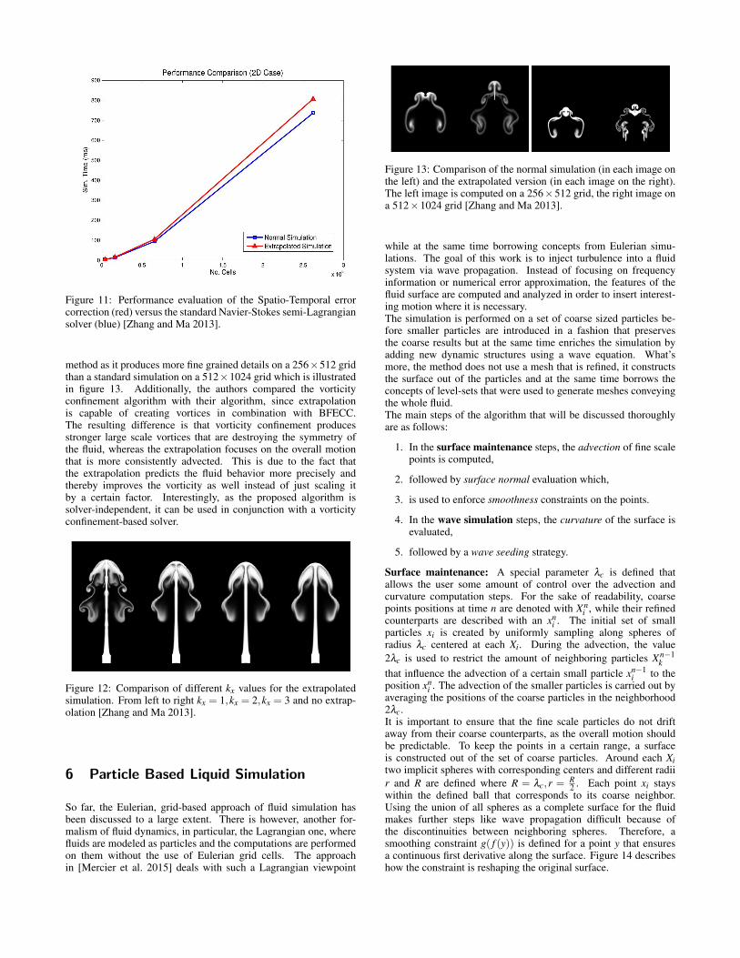
Figure 11: Performance evaluation of the Spatio-Temporal errorcorrection (red) versus the standard Navier-Stokes semi-Lagrangiansolver (blue) [Zhang and Ma 2013].

method as it produces more fine grained details on a 256×512 gridthan a standard simulation on a 512×1024 grid which is illustratedin figure 13. Additionally, the authors compared the vorticityconfinement algorithm with their algorithm, since extrapolationis capable of creating vortices in combination with BFECC.The resulting difference is that vorticity confinement producesstronger large scale vortices that are destroying the symmetry ofthe fluid, whereas the extrapolation focuses on the overall motionthat is more consistently advected. This is due to the fact thatthe extrapolation predicts the fluid behavior more precisely andthereby improves the vorticity as well instead of just scaling itby a certain factor. Interestingly, as the proposed algorithm issolver-independent, it can be used in conjunction with a vorticityconfinement-based solver.

Figure 12: Comparison of different kx values for the extrapolatedsimulation. From left to right kx = 1,kx = 2,kx = 3 and no extrap-olation [Zhang and Ma 2013].

6 Particle Based Liquid Simulation

So far, the Eulerian, grid-based approach of fluid simulation hasbeen discussed to a large extent. There is however, another for-malism of fluid dynamics, in particular, the Lagrangian one, wherefluids are modeled as particles and the computations are performedon them without the use of Eulerian grid cells. The approachin [Mercier et al. 2015] deals with such a Lagrangian viewpoint

Figure 13: Comparison of the normal simulation (in each image onthe left) and the extrapolated version (in each image on the right).The left image is computed on a 256×512 grid, the right image ona 512×1024 grid [Zhang and Ma 2013].

while at the same time borrowing concepts from Eulerian simu-lations. The goal of this work is to inject turbulence into a fluidsystem via wave propagation. Instead of focusing on frequencyinformation or numerical error approximation, the features of thefluid surface are computed and analyzed in order to insert interest-ing motion where it is necessary.The simulation is performed on a set of coarse sized particles be-fore smaller particles are introduced in a fashion that preservesthe coarse results but at the same time enriches the simulation byadding new dynamic structures using a wave equation. What’smore, the method does not use a mesh that is refined, it constructsthe surface out of the particles and at the same time borrows theconcepts of level-sets that were used to generate meshes conveyingthe whole fluid.The main steps of the algorithm that will be discussed thoroughlyare as follows:

1. In the surface maintenance steps, the advection of fine scalepoints is computed,

2. followed by surface normal evaluation which,

3. is used to enforce smoothness constraints on the points.

4. In the wave simulation steps, the curvature of the surface isevaluated,

5. followed by a wave seeding strategy.

Surface maintenance: A special parameter λc is defined thatallows the user some amount of control over the advection andcurvature computation steps. For the sake of readability, coarsepoints positions at time n are denoted with Xn

i , while their refinedcounterparts are described with an xn

i . The initial set of smallparticles xi is created by uniformly sampling along spheres ofradius λc centered at each Xi. During the advection, the value2λc is used to restrict the amount of neighboring particles Xn−1

kthat influence the advection of a certain small particle xn−1

i to theposition xn

i . The advection of the smaller particles is carried out byaveraging the positions of the coarse particles in the neighborhood2λc.It is important to ensure that the fine scale particles do not driftaway from their coarse counterparts, as the overall motion shouldbe predictable. To keep the points in a certain range, a surfaceis constructed out of the set of coarse particles. Around each Xitwo implicit spheres with corresponding centers and different radiir and R are defined where R = λc,r = R

2 . Each point xi stayswithin the defined ball that corresponds to its coarse neighbor.Using the union of all spheres as a complete surface for the fluidmakes further steps like wave propagation difficult because ofthe discontinuities between neighboring spheres. Therefore, asmoothing constraint g( f (y)) is defined for a point y that ensuresa continuous first derivative along the surface. Figure 14 describeshow the constraint is reshaping the original surface.

Figure 14: The defined surface within R and r (blue dots) is con-strained to a continuous function (from green to red) [Mercier et al.2015].

In order to simulate waves, the distribution of the points xi mustbe improved. To achieve this goal, normals ni for each xi arecomputed via fitting a plane onto the smooth surface. Each particleis now displaced along its normal where the amount depends onthe placement of its neighbors xk in a radius λc. The idea behindthis step is to reposition outliers such that no unusual bumps occurwhen the particles are fused to a common fluid surface. Thepoint distribution is improved by moving each xi away from theirneighbors along x′is tangent plane. In addition, points are deleted ifthe density is too high, or inserted if there is not a sufficient amountof neighbors present.

Wave Simulation: With the previous steps a scenario is cre-ated that allows for additional turbulence propagation, the key stepin this algorithm. The idea is that waves should always form inregions where many particles collide or separate. Such regionscan be identified by computing the mean curvature for each point.As a tangent plane has been established previously, the value thatcan be compared to mean curvature is defined as the distance ofx′is neighbors from the tangent plane of particle i and called ci. A

Figure 15: Wave seeding strategy on a high curvature region[Mercier et al. 2015].

wave traveling along the surface will be amplified if the value ofci is high enough. The authors first compute an amplitude ai thatdepends on the mean curvature and subsequently add up multiplecosine functions, multiplied by ai, that have a certain frequencyrange provided by the user. The result of the addition is stored in si.The algorithm then solves a wave equation with the si values addedto the height of the current wave di resulting in a new height hi(Figure 15 middle in red). It has to be ensured that only frequenciesare displayed that actually propagate out of the wave, therefore,hi is never displayed. Instead, di is recomputed after solving thewave equation with hi ,by subtracting si from the newly obtainedhi. In figure 15, this behavior is displayed. The left image showsthe values hi and di without any amplification. In the middle, si isshown after amplification together with hi. The subtraction aftersolving the wave equation is shown in green on the right. Thedashed green line symbolizes the wave propagation if no additionalfrequencies would have been added. As an additional step, theauthors never use the Laplace-Beltrami operator to solve thewave equations, instead, they approximate it with a flat Laplacianthat has proven to yield more stable results. Furthermore, thecomputational cost is reduced by this approximation.

Results and Performance: The authors compared their methodto a standard particle solver that does not perform upsamplingsteps. Figure 16 shows a simulation with 12.5 million particleson the left. On top of this simulation the authors generate 500000

fine surface points and apply their wave evolution strategy. It isimmediately visible that the resulting image on the right conveysmore fine structured details where the original surface has a moresmooth structure. It is remarkably that the simulation can still beimproved even if it contains a large amount of particles.In Figure 17 a scenario is shown where the flow follows a riverbedwith obstacles in between. The standard simulation has 400000particles and the upsampled version adds another 280000 smallscaled surface points. The amount of additional detail is immedi-ately visible.In Figure 18 a high resolution solver (left) with 4 million particlesis compared to the discussed algorithm operating on a lowerresolution of 2500 coarse particles and 15500 small particles. Thedevised algorithm yields sharper waves and is also more efficientto compute since the high resolution simulation took 142s/frame incomparison to 4.74s/frame for the new method.The authors use a hash structure for speeding up the lookupsalong the neighborhood region. With this, the simulation is 200times faster on 290000 particles in comparison to iterating overall particles for finding neighbors. Furthermore, since most ofthe computations on the surface points are independent from eachother, OpenMP is used to further accelerate the algorithm makingthe affected operations 8 times faster.

Figure 16: Wave seeding strategy on a high curvature region[Mercier et al. 2015].

Figure 17: Wave seeding strategy on a high curvature region[Mercier et al. 2015].

Figure 18: Wave seeding strategy on a high curvature region[Mercier et al. 2015].

7 Adaptive Simulation

The procedure in [Ando et al. 2013] tackles the upsampling prob-lem in various ways. As discussed, using a uniform, Eulerian grid,is infeasible since it cannot focus on interesting motion and resolveit in more detail while at the same time wasting computationalresources at places where the fluid motion is uninteresting andthe calculations could be performed more coarsely. The authorstherefore devised a solver which operates on a tetrahedral mesh.This structure is adaptively refined, depending on where interestingmotion occurs. The algorithm is of hybrid nature, meaning thatit still follows an Eulerian approach because the pressure andvelocity is stored on the tetrahedral cells, but at the same timeit uses particles from which a surface is computed. In the past,similar methods have been established using octrees, however, theauthors in [Ando et al. 2013] denote that this approach still suffersfrom numerical errors and tetrahedral meshes are superior.

Fluid Solver: On each triangle of the mesh, a 3 dimensionalvelocity vector is stored at the cells center and a pressure valueis stored on each vertex of the triangle. This setup allows thecomputation of the Poisson projection step modeled in equation 11in an efficient and robust fashion. The energy minimization ofthe Poisson equation is modeled as a linear m× n system, wherem is the number of tetrahedra and n is the number of nodes. Asthe number of nodes is always smaller than n, this system canbe solved fast and without artifacts. Artifacts appear when moredegrees of freedom for the pressure values are possible than for thevelocities. By construction, this method prevents such a scenarioas the authors claim, although a formal proof has not been given.Similar to [Mercier et al. 2015], the algorithm employs a positioncorrection step where particles are moved away from its neighborsalong the tangential direction of the surface. In order to preventholes by using this correction, particles that lie underneath thesurface will also be pushed towards the boundary of the surface,filling up empty space left behind. As an additional improvement,particles that move freely in space outside of the fluids boundary(for example, when splashes occur) will be excluded from thepressure solver and only gravitational forces are then applied tothem as there are zero internal forces present in such cases.

Adaptivity: The adaptive component in the simulation is thetetrahedral mesh, which is recomputed every 10 time steps.The establishment of a tetrahedral mesh follows the algorithmfrom [Labelle and Shewchuk 2007]. During the recomputationof the mesh, all particles are inspected individually and it isdetermined whether they are either to big or too small. A particleis merged with a neighbor if it is too small. In the opposite case, aparticle will be split and two new particles are formed in a way thattries to fill the gaps between their neighbors.The crucial step is to determine when a split or merge operationneeds to occur. To determine this, a special sizing function hasbeen devised:

S(x) = max(d(x),V (x,min(κliquid(x),κsolid(x),e(x)))). (33)

In this equation, d(x) is the distance of the particle from the surfaceof the wave. Motion near the surface must be modeled more pre-cisely than motion farther below. V (x,y) is a function that returnsy if the point is inside the view frustum, otherwise, the result is themaximum allowed particle radius. The value y results form 3 dif-ferent computations. The curvature is represented by κliquid(x), thehigher this value, the smaller the particle radius should be and viceversa. The distance to the nearest solid object is smoothly evaluated

by κsolid(x) with respect to the maximum radius:

κsolid(x) = 1.6

((1−‖dsolid‖2)

r2max

)3

, (34)

where dsolid is the distance to the solid object and rmax is themaximum radius. The idea is that particles near the solid objectmust be modeled more fine grained. The function e(x) evaluatesthe strain tensor of the velocity field. This tensor describes the rateof change in velocities around a certain point and therefore conveysinformation about parts in the flow that convey interesting motion.

Surface Representation: The authors also propose a newmethod for representing the surface. This is necessary as previousmethods can not handle many particles with such an ampledifference in their radii. The final displayed surface is composedof the union of convex hulls that are formed by 3 neighboringparticles that are close to the surface border. For the convexhull candidates, only particles that are lesser than l times thesum of the surface points and its neighbors radius apart areconsidered. A small l allows for the depiction of more details,that might be too bumpy and a large l smooths out concavities.The authors used l = 2 for most of their simulations, the convexhull of three particles is shown in Figure. After the surface hasbeen established, the level set value from each vertex in themesh is then computed. The resulting surface however, is ex-pensive to compute with an average runtime of 5 minutes per frame.

Results and Performance: The most remarkable result ofthis algorithm can be analyzed in Figure 19, where a scene isdepicted that would be difficult to compute with a standard solver.The fine details that occur within the splashes could otherwiseonly be achieved with a very fine grid. The authors note that aresolution of 400 million particles would have been needed toobtain the same accuracy as they achieved on the finest level ofadaptivity. In comparison their method used 1.7 million particles,small scale details can be captured because of the sizing function.On average, the simulation took 4.6 seconds per frame, althoughit is presumed that the authors left out the time for the surfacecomputation otherwise they would contradict themselves. Infigure 20, another scene is shown that demonstrates the adaptivityof the method. The complex obstacle in the middle creates variousamounts of distortion in the flow and the method is able to capturethis by refining the particle size in regions around the obstacle.Regarding possible performance improvements, the authors statethat the mesh generation also poses a performance bottleneck intheir simulations as it can not parallelized. Further drawbacks arethe configuration of the sizing function. There are constants thatare not optimized perfectly and artifacts can occur in small areaswhen particle sizes vary too much. Furthermore, their method isnot proven to behave correctly when viscosity and diffusion ismodeled and the authors note that difficulties could arise in thesecases. The repositioning of particles is also not entirely physicallyaccurate but a necessity as a configuration could result that hasmore particles in a certain area than velocity samples in the grid.This would also lead to artifacts.

8 Comparison and Conclusion

In summary, all methods that have been discussed in detail try toimprove fluid simulations on some level. The wavelet turbulencemethod, together with vorticity confinement add motion to a fluidin a procedural fashion that is not entirely physically accurate but

Figure 19: A scene that is difficult to evaluate precisely with nonadaptive simulations because highly detailed splashes occur whenthe objects begin to flow and drop into the water [Ando et al. 2013].

Figure 20: This scene depicts a obstacle with small an big holes thatcreate small scale splashes and swirling motions when the waterflows through it. Therefore an adaptive simulation that refines theresolution in this area is beneficial [Ando et al. 2013].

yields convincing visual results. In contrast, the higher order ad-vection solvers together with the spatio-temporal method providea purely numerical refinement that is closer to physical reality butthe freedom of finetuning certain parameters may not be as pleas-ing. The hybrid approaches try to combine Eulerian and Lagrangiansimulations and also apply some regularizations that have no realphysical meaning, nevertheless they are also able to achieve a con-vincing amount of added small scale detail. The approaches allhave their benefits and drawbacks, it is crucial to understand thatdifferent scenarios require different techniques. Each technique of-fers a huge amount of improvement compared to non-upsamplingstandard solvers, both in computational complexity as well as in thevisual results that can be achieved.

8.1 Comparison of the Particle Based Solvers

Concerning the Particle-based solvers, the adaptive simulationmight present superior simulations, while the Surface turbulencemethod might not be able to model fine details as accurate. Whenconcerning the performance, the latter approach might be more con-venient for artists. The authors mention that the framerate, evenon complex scenes is always below 1 minute, this superiority incomparison with the adaptive simulation allows for a more rapiddevelopment process, which might be favored by artists. After apreferred scene has been established, one can choose to refine thesimulation by employing the adaptive solver. It should also be notedthat the adaptive version might not be able to simulate small waves

in areas that are underresolved because the sizing function doesnot refine certain areas that are determined to convey little activ-ity. When analyzing the right image in figure 18 small turbulentwaves are simulated in areas that have only minor curvatures, thehighly adaptive version might not be able to capture such detailsand is certainly not able to simulate additional waves.

8.2 Comparison of Particle Based solvers andWavelet turbulence

Because of the wave seeding strategy the approach in [Mercier et al.2015] can be compared to the wavelet turbulence algorithm [Kimet al. 2008]. Both methods inject turbulence at certain frequencybands, it is however not known how the simulation in [Mercieret al. 2015] behaves on scenarios where the motion of smoke ismodeled. According to [Stam 2003], particle based methods arenot able to capture the fine grained motions of smoke without usingmany particles. Because [Mercier et al. 2015] uses coarse parti-cles as the underlying starting point for further refinement, the sizeof those particles might pose a restriction on the amount of finegrained turbulence in smoke simulations as for example in figure 9.Therefore, the method of choice when computing smoke simula-tions would be the wavelet turbulence approach, the higher orderadvection solvers or the spatio-temporal extrapolation method. It isnot known whether the adaptive simulation on tetrahedral meshesis superior to the wavelet turbulence algorithm or not. The authorsstate that the applicability of the method with regards to smoke sim-ulation is still a topic of further research. However, similar con-clusions as mentioned above can be drawn. Although the parti-cle size is refined in areas of interesting motion it is not clear ifthe adaption can correctly consider forward and backward scatter-ing effects. It would be interesting to employ an adaptive waveletturbulence sceme where the application refines a mesh based com-putation upon the detection of scattering effects. Furthermore, thewavelet turbulence method is not able to exactly reproduce simula-tions on very high resolution grids. Similar to the surface turbulenceapproach, the wavelet turbulence results are dependent on the lowresolution simulations when obstacles are within the flow.

8.3 Comparison of Wavelet turbulence with numer-ical error correction based solvers

The wavelet turbulence method might allow more freedom whendesigning simulations, because the number of frequency bands thatare added can be defined manually, depending on the needs of theartist. Simulations that focus solely on the improvement of numer-ical error terms such as BFECC, the MacCormack method and alsothe Spatio-Temporal extrapolation will always produce the same re-sult. Still these approaches are highly valuable when there is needfor physical accuracy since they do not add additional turbulencewhich is not entirely physically accurate. Such scenarios couldbe wind tunnel simulations for example. In addition, algorithmsthat focus on numerical improvements can be combined in order toachieve an even better result in a satisfactorily amount of time asdiscussed in [Zhang and Ma 2013].

References

ANDO, R., THUREY, N., AND WOJTAN, C. 2013. Highly adaptiveliquid simulations on tetrahedral meshes. ACM Transactions onGraphics (TOG) 32, 4, 103.

B. KIM, Y. LIU, I. L. J. R. 2005. Flowfixer: Using bfecc for fluidsimulation. In Proceedings of the Eurographics Work shop onNatural Phenomena.

COHEN, L. 1995. Time-frequency Analysis: Theory and Applica-tions. Prentice-Hall, Inc., Upper Saddle River, NJ, USA.

COOK, R. L., AND DEROSE, T. 2005. Wavelet noise. ACM Trans.Graph. 24, 3 (July), 803–811.

DUPONT, T. F., AND LIU, Y. 2003. Back and forth error com-pensation and correction methods for removing errors inducedby uneven gradients of the level set function. Journal of Compu-tational Physics 190, 1, 311–324.

FEDKIW, R., STAM, J., AND JENSEN, H. W. 2001. Visual simu-lation of smoke. In Proceedings of the 28th Annual Conferenceon Computer Graphics and Interactive Techniques, ACM, NewYork, NY, USA, SIGGRAPH ’01, 15–22.

KIM, T., THUREY, N., JAMES, D., AND GROSS, M. 2008.Wavelet turbulence for fluid simulation. In ACM Transactionson Graphics (TOG), vol. 27, ACM, 50.

LABELLE, F., AND SHEWCHUK, J. R. 2007. Isosurface stuffing:Fast tetrahedral meshes with good dihedral angles. ACM Trans-actions on Graphics 26, 3 (July), 57.1–57.10. Special issue onProceedings of SIGGRAPH 2007.

MERCIER, O., BEAUCHEMIN, C., THUEREY, N., KIM, T., ANDNOWROUZEZAHRAI, D. 2015. Surface turbulence for particle-based liquid simulations. ACM Transactions on Graphics (Pro-ceedings of ACM SIGGRAPH Asia 2015) 34, 6 (Nov.).

PERLIN, K., AND VELHO, L. 1995. Live paint: Painting with pro-cedural multiscale textures. In Proceedings of the 22Nd AnnualConference on Computer Graphics and Interactive Techniques,ACM, New York, NY, USA, SIGGRAPH ’95, 153–160.

SELLE, A., FEDKIW, R., KIM, B., LIU, Y., AND ROSSIGNAC, J.2008. An unconditionally stable maccormack method. Journalof Scientific Computing 35, 2-3, 350–371.

STAM, J. 1999. Stable fluids. In Proceedings of the 26th An-nual Conference on Computer Graphics and Interactive Tech-niques, ACM Press/Addison-Wesley Publishing Co., New York,NY, USA, SIGGRAPH ’99, 121–128.

STAM, J. 2003. Real-time fluid dynamics for games. In Proceed-ings of the game developer conference, vol. 18, 25.

ZHANG, Y., AND MA, K.-L. 2013. Spatio-temporal extrapolationfor fluid animation. ACM Transactions on Graphics (TOG) 32,6, 183.

ZSOLNAI, K., AND SZIRMAY-KALOS, L. Real-time simulationand control of newtonian fluids using the navier-stokes equa-tions.