Eur. Phys. J. C (2019) 79:1032https://doi.org/10.1140/epjc/s10052-019-7542-5

Regular Article - Theoretical Physics

Upper limits on the amplitude of ultra-high-frequencygravitational waves from graviton to photon conversion

A. Ejlli1,a , D. Ejlli3, A. M. Cruise2, G. Pisano1, H. Grote1

1 School of Physics and Astronomy, Cardiff University, The Parade, Cardiff CF24 3AA, UK2 School of Physics and Astronomy, Birmingham University, Edgbaston Park Rd, Birmingham B15 2TT, UK3 Department of Physics, Novosibirsk State University, 2 Pirogova Street, Novosibirsk 630090, Russia

Received: 28 September 2019 / Accepted: 9 December 2019 / Published online: 26 December 2019© The Author(s) 2019

Abstract In this work, we present the first experimen-tal upper limits on the presence of stochastic gravitationalwaves in a frequency band with frequencies above 1 THz.We exclude gravitational waves in the frequency bands from(2.7 − 14) × 1014 Hz and (5 − 12) × 1018 Hz down to acharacteristic amplitude of hmin

c ≈ 6 × 10−26 and hminc ≈

5 × 10−28 at 95% confidence level, respectively. To obtainthese results, we used data from existing facilities that havebeen constructed and operated with the aim of detectingweakly interacting slim particles, pointing out that thesefacilities are also sensitive to gravitational waves by gravi-ton to photon conversion in the presence of a magnetic field.The principle applies to all experiments of this kind, withprospects of constraining (or detecting), for example, gravi-tational waves from light primordial black-hole evaporationin the early universe.

1 Introduction

With the first detections of gravitational waves (GWs) bythe ground-based laser interferometers LIGO and VIRGO,a new tool for astronomy, astrophysics and cosmology hasbeen firmly established [1,2]. GWs are spacetime perturba-tions predicted by the theory of general relativity that propa-gate with the speed of light and can be predominantly char-acterised by their frequency f and the dimensionless (char-acteristic) amplitude hc. Based on these two quantities andthe abundance of sources across the full gravitational-wavespectrum, as well as the availability of technology, it becomesclear that different parts of the gravitational-wave spectrumare more accessible than others.

Current ground-based detectors are sensitive in the fre-quency band from about 10 Hz to 10 kHz [3–6] where the

a e-mail: EjlliA@cardiff.ac.uk

intersection of efforts in the development of the technologyand the abundance of sources facilitated the first detections.Coalescences of compact objects such as black holes andneutron stars have been detected, and spinning neutron stars,supernovae and stochastic signals are likely future sources.Since in principle, GWs can be emitted at any frequency, theyare expected over many decades of frequency below the audioband, but also above it. At lower frequencies, the space-basedlaser interferometer LISA is firmly planned to cover the 0.1–10 mHz band [7,8], targeting, for example, black-hole andwhite-dwarf binaries. At even lower frequencies in the nHzregime, the pulsar timing technique promises to facilitatedetections of GWs from supermassive black holes [9–11].

Frequencies above 10 kHz have been much less in thefocus of research and instrument development in the past, butgiven the blooming of the field, it seems appropriate to notlose sight of this domain as technology progresses. One of themain reasons to look for such high frequencies of GWs is thatseveral mechanisms that generate very-high-frequency GWsare expected to have occurred in the early universe just afterthe big bang. Therefore, the study of such frequency bandswould give us a unique possibility to probe the very earlyuniverse. However, the difficulty in probing such frequencybands is explained by the fact that laser-interferometric detec-tors such as LIGO, VIRGO and LISA work in the lower fre-quency part of the spectrum and their working technology isnot necessarily ideal for studying very-high-frequency GWs.The characteristic amplitude of a stochastic background ofGWs hc, for several models of GW generation, decreases asthe frequency f increases. Consequently, to study GWs withfrequencies in the GHz regime or higher requires highly sen-sitive detectors in terms of the characteristic amplitude hc.

One possible way to construct detectors for very-high-frequency GWs is to make use of the partial conversion ofGWs into electromagnetic waves in a magnetic field. Indeed,as general relativity in conjunction with electrodynamics pre-

123

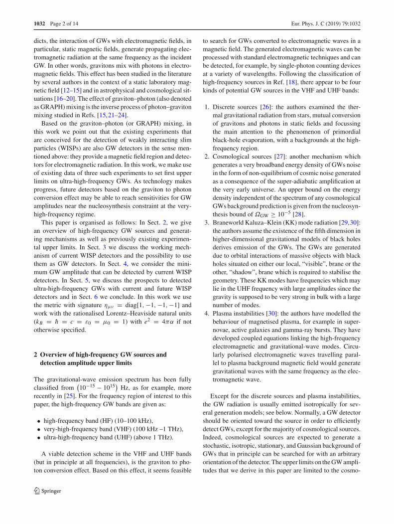
1032 Page 2 of 14 Eur. Phys. J. C (2019) 79 :1032

dicts, the interaction of GWs with electromagnetic fields, inparticular, static magnetic fields, generate propagating elec-tromagnetic radiation at the same frequency as the incidentGW. In other words, gravitons mix with photons in electro-magnetic fields. This effect has been studied in the literatureby several authors in the context of a static laboratory mag-netic field [12–15] and in astrophysical and cosmological sit-uations [16–20]. The effect of graviton–photon (also denotedas GRAPH) mixing is the inverse process of photon–gravitonmixing studied in Refs. [15,21–24].

Based on the graviton–photon (or GRAPH) mixing, inthis work we point out that the existing experiments thatare conceived for the detection of weakly interacting slimparticles (WISPs) are also GW detectors in the sense men-tioned above: they provide a magnetic field region and detec-tors for electromagnetic radiation. In this work, we make useof existing data of three such experiments to set first upperlimits on ultra-high-frequency GWs. As technology makesprogress, future detectors based on the graviton to photonconversion effect may be able to reach sensitivities for GWamplitudes near the nucleosynthesis constraint at the very-high-frequency regime.

This paper is organised as follows: In Sect. 2, we givean overview of high-frequency GW sources and generat-ing mechanisms as well as previously existing experimen-tal upper limits. In Sect. 3 we discuss the working mech-anism of current WISP detectors and the possibility to usethem as GW detectors. In Sect. 4, we consider the mini-mum GW amplitude that can be detected by current WISPdetectors. In Sect. 5, we discuss the prospects to detectedultra-high-frequency GWs with current and future WISPdetectors and in Sect. 6 we conclude. In this work we usethe metric with signature ημν = diag[1,−1,−1,−1] andwork with the rationalised Lorentz–Heaviside natural units(kB = h = c = ε0 = μ0 = 1) with e2 = 4πα if nototherwise specified.

2 Overview of high-frequency GW sources anddetection amplitude upper limits

The gravitational-wave emission spectrum has been fullyclassified from

(10−15 − 1015

)Hz, as for example, more

recently in [25]. For the frequency region of interest to thispaper, the high-frequency GW bands are given as:

• high-frequency band (HF) (10–100 kHz),• very-high-frequency band (VHF) (100 kHz –1 THz),• ultra-high-frequency band (UHF) (above 1 THz).

A viable detection scheme in the VHF and UHF bands(but in principle at all frequencies), is the graviton to pho-ton conversion effect. Based on this effect, it seems feasible

to search for GWs converted to electromagnetic waves in amagnetic field. The generated electromagnetic waves can beprocessed with standard electromagnetic techniques and canbe detected, for example, by single-photon counting devicesat a variety of wavelengths. Following the classification ofhigh-frequency sources in Ref. [18], there appear to be fourkinds of potential GW sources in the VHF and UHF bands:

1. Discrete sources [26]: the authors examined the ther-mal gravitational radiation from stars, mutual conversionof gravitons and photons in static fields and focussingthe main attention to the phenomenon of primordialblack-hole evaporation, with a backgrounds at the high-frequency region.

2. Cosmological sources [27]: another mechanism whichgenerates a very broadband energy density of GWs noisein the form of non-equilibrium of cosmic noise generatedas a consequence of the super-adiabatic amplification atthe very early universe. An upper bound on the energydensity independent of the spectrum of any cosmologicalGWs background prediction is given from the nucleosyn-thesis bound of ΩGW ≥ 10−5 [28].

3. Braneworld Kaluza–Klein (KK) mode radiation [29,30]:the authors assume the existence of the fifth dimension inhigher-dimensional gravitational models of black holesderives emission of the GWs. The GWs are generateddue to orbital interactions of massive objects with blackholes situated on either our local, “visible”, brane or theother, “shadow”, brane which is required to stabilise thegeometry. These KK modes have frequencies which maylie in the UHF frequency with large amplitudes since thegravity is supposed to be very strong in bulk with a largenumber of modes.

4. Plasma instabilities [30]: the authors have modelled thebehaviour of magnetised plasma, for example in super-novae, active galaxies and gamma-ray bursts. They havedeveloped coupled equations linking the high-frequencyelectromagnetic and gravitational-wave modes. Circu-larly polarised electromagnetic waves travelling paral-lel to plasma background magnetic field would generategravitational waves with the same frequency as the elec-tromagnetic wave.

Except for the discrete sources and plasma instabilities,the GW radiation is usually emitted isotropically for sev-eral generation models; see below. Normally, a GW detectorshould be oriented toward the source in order to efficientlydetect GWs, except for the majority of cosmological sources.Indeed, cosmological sources are expected to generate astochastic, isotropic, stationary, and Gaussian background ofGWs that in principle can be searched for with an arbitraryorientation of the detector. The upper limits on the GW ampli-tudes that we derive in this paper are limited to the cosmo-

123

Eur. Phys. J. C (2019) 79 :1032 Page 3 of 14 1032

logical sources since the detectors (see next section), exceptfor one experiment which pointed towards the sun, cannotpoint deliberately to the emitting sources, so their measure-ments are most sensitive to sources creating an isotropicbackground of GWs. We list some possible sources of GWs:

1. Stochastic background of GWsThe stochastic background of GWs is assumed to beisotropic [28,31,32] and must exist at present as a resultof an amplification of vacuum fluctuations of gravita-tional field to other mechanisms that can take place dur-ing or after inflation [33]. Inflationary processes and thehypothetical cosmic strings are potential candidates ofthe GW background with some differences in the pre-dicted intensity and spectral features [28,31,32]. Thesespectrum would have cutoff frequency approximately inthe region νc ∼ 1011 Hz. The prediction for the cutofffrequency in some cosmic string models gives the cutoffshifted to 1013 − 1014 Hz [28,31,32]. The metric pertur-bation at the cutoff frequency 1011 Hz corresponds to anestimated strain amplitude of hc ∼ 10−32.

2. GWs from primordial black holesIn Ref. [34], the authors proposed the existence of primor-dial black-hole (PBH) binaries and estimated the radiatedGW spectrum from the coalescence of such binaries. Inaddition, the mechanism of evaporation of small massblack holes gives rise to the production of high and ultra-high-frequency GWs. An estimation of the efficiency ofthis emission channel which might compensate the deficitof high-frequency gravitons in the relic GW backgroundhas been thoroughly studied in [26]. A detailed calcula-tion of the energy density of relic GWs emitted by PBHshas been performed in [35]. The author’s analysed andcalculated the energy density of GWs from PBH scatter-ing in the classical and relativistic regimes, PBH binarysystems, and PBH evaporation due to the Hawking radi-ation.

3. GWs from thermal activity of the sunA third class that does generate a stochastic, but not anisotropic background of GWs, which is relevant to thiswork, is the GW emission from the sun [36]. The hightemperature of the sun in the proton–electron plasma pro-duces isotropic gravitational radiation noise due to ther-mal motion [37–39]. The emission comes to the detec-tor from the direction of the sun, and the observationshave the potential to set limits on this process. The fre-quency of the collisions of νc ∼ 1015 Hz determines thegravitational-wave frequency, and the highest frequencycorresponds to the thermal limit at ωm = kT/h ∼ 1018

Hz. Using the plasma parameters in the centre of theSun the estimation of the “thermal gravitational noise ofthe Sun” reaching the earth provides a stochastic flux at“optical frequencies” of the order hc ∼ 10−41 [39].

So far, dedicated experiments to detect GWs in the VHFregion are based on two designs: polarisation measurementon a cavity/waveguide detector and cross-correlation mea-surement of two laser interferometers. The cavity/waveguideprototype measured polarisation changes of the electromag-netic waves, which in principle can rotate under an incomingGW, providing an upper limit on the existence of GWs back-ground to a dimensionless amplitude of hc ≤ 1.4 × 10−10 at100 MHz [40]. The two laser interferometer detectors with0.75 m long arms have used a so-called synchronous recy-cling interferometer and provided an upper limit on the exis-tence of the GW background to a dimensionless amplitudeof hc ≤ 1.4 × 10−12 at 100 MHz [41,42].

The most recent upper limit on stochastic VHF GWs hasbeen set by a graviton–magnon detector which measures res-onance fluorescence of magnons [44]. One used experimentalresults of the axion dark matter using magnetised ferromag-netic samples to derive the upper limits on stochastic GWswith characteristic amplitude hc ≤ 9.1 × 10−17 at 14 GHzand hc ≤ 1.1 × 10−15 at 8.2 GHz.

Another facility, the Fermilab Holometer, has performedmeasurement at slightly lower frequencies. The FermilabHolometer [43] consists of separate, yet identical Michel-son interferometers, with 39 m long arms. The upper limitsfound within 3σ , on the amplitude of GWs are in the rangehc < 25 × 10−19 at 1 MHz down to a hc < 2.4 × 10−19 at13 MHz.

3 WISP search experiments and their relevance to UHFGWs

The experiments ALPS [45], OSQAR [46] and CAST [36]have not been designed to detect GWs in the first place. How-ever, in this work their results are used to compute new upperlimits on GW amplitudes and related parameters. The exper-iments performed by ALPS and OSQAR are usually called“light shining through the wall experiment” where the hypo-thetical WISPs, that are generated within the experiment,mediate the “shining through the wall” process, and decayingsuccessively into photons. In contrast, the CAST experimentsearches directly for WISPs emitted from the core of the sun.Though all these experiments are not designed to detect grav-itational waves, they provide a high sensitivity measurementof single photons generated in their constant magnetic fieldwhich is the crucial ingredient for the detection of gravitonto photon conversion.

The main characteristics of the ALPS, OSQAR and CASTexperiments are:

1. ALPS experiment at DESYThe ALPS (I) experiment has performed the last datataking run in 2010, and the specific characteristics of the

123

1032 Page 4 of 14 Eur. Phys. J. C (2019) 79 :1032

Fig. 1 Simplified schematic of the experimental setup aiming at thedetection of WISPs. In the upper panel left-hand side, the electromag-netic waves interacting with the magnetic field produce the hypotheticalWISPs, and at the right-hand side electromagnetic waves are producedby the decay of WISPs in the constant magnetic field. Our work is illus-trated by the lower panel ignoring the transparent left-hand side. Onthe right-hand side, the photons detected could be due to the passage ofGWs propagating in the constant magnetic field

experiment are found in Ref. [47]. A general schematicof the principle is shown in the upper panel of Fig. 1.The production of WISPs and their re-conversion intoelectromagnetic radiation is located in one single HERAsuperconducting magnet where an opaque wall in themiddle separates the two processes. The HERA dipoleprovides a magnetic field of 5 T in a length of 8.8 m. Theelectromagnetic radiation, generated by the decay of theWISPs in the magnetic field, passed a lens of 25.4 mmdiameter and focal length 40 mm. The lens focusses thelight onto a ≈ 30 μm diameter beam spot on a CCDcamera.

2. OSQAR experiment at CERNThe OSQAR experiment has performed the last data tak-ing in 2015, and the specific characteristics of the exper-imental setup are found in [46,48]. The OSQAR col-laboration has used two LHC superconducting dipolemagnets separated by an optical barrier (for a concep-tual scheme see the upper panel of the Fig. 1). The LHCdipole magnets provide a constant magnetic field of 9 T,along a length of 14.3 m. To focus the generated photonsof the beam onto the CCD, an optical lens of 25.4 mmdiameter and a focal length of 100 mm was used, installedin front of the detector similar to Fig. 1. Data acquisitionhas been performed in two runs with two different CCD’shaving different quantum efficiencies.

3. CAST experiment at CERNThe CERN Axion Solar Telescope (CAST) experimenthas the aim to detect or set upper limits on the flux ofthe hypothetical low-mass WISPs produced by the Sun.A refurbished CERN superconducting dipole magnet of9 T and 9 m length was used. The solar axions with

expected energies in the keV range can convert into X-rays in the constant magnetic field, and an X-ray detec-tor has been used to performed runs in the time period2013–2015 [49]. To increase the cross-section, the twoparallel pipes which pass through the magnet both havebeen used which provide an area of 2×14.5 cm2 focussedinto a Micromegas detector. The CAST detector mountedon the pointing system had a telescope with a focallength of 1.5 m installed for the (0.5 – 10) keV energyrange.

4 Minimal-detection of GW amplitude

In this section, we show how we compute upper limits onthe GW dimensionless amplitude hc based on the character-istics of the experiments described above that are sensitive toan isotropic background of GWs from cosmological sourcesand to the thermal activity in the sun. We ignore the genera-tion of WISPs (Fig. 1: lower panel) and focus on the secondhalf of the magnetic field for the case of ALPS and OSQARexperiments, and, for the CAST experiment we consider thefull magnet region. These experiments measure a numberof photons per unit time with their CCD detectors, namelyNexp in an energy band Δω with efficiency εγ and in a cross-section A. In what follows we assume that in the CCD thebackground dark current fluctuation is a stochastic processwith uniform probability distribution and being stationary inω. In this case, the energy flux of photons generated in anenergy bandwidth [ωi , ω f ] is given by

ΦCCDγ

(z, ω f ; t

) =∫ ω f

ωi

1

A (z)

N (ω, t) ω

εγ (ω)dω (1)

where N (ω, t) is the number of photons per unit of time andenergy. Now, we have to compare the measured energy fluxof photons with the intrinsic energy flux of photons gener-ated in the graviton to photon conversion in the presence ofan isotropic background of GWs. The analytical treatmentfor an isotropic background of GWs converted into electro-magnetic waves, is described in detail in Appendices 2 and3. In Appendix 3, different useful quantities are calculated,for stochastic GWs propagating in a transverse and constantmagnetic field. Since all the experiments operated under vac-uum condition and the propagation distance z is small withrespect to the oscillation length of the particles, we can safelytake Δx,y z � 1. The variable Δx,y defined in Eq. (A.7) is afunction of the magnetic field, the magnitudes of the photonand graviton wave-vectors and the Newton constant. Thenthe energy flux of photons generated in the magnetic field oflength z given by Eq. (B.16), in the same energy bandwidth[ωi , ω f ], becomes

123

Eur. Phys. J. C (2019) 79 :1032 Page 5 of 14 1032

Φgraphγ

(z, ω f ; t

) =(Mx

gγ

)2∫ ω f

ωi

[sin2 (Δx z)

Δ2x

+ sin2 (Δy z

)

Δ2y

]

×h2c (0, ω) ω

2 κ2 dω

�∫ ω f

ωi

B2 z2 h2c (0, ω) ω

4. (2)

Comparing the energy fluxes in Eqs. (1) and (2), andrequiring that, for detection, the energy flux in (2) must bebigger than or equal to the energy flux in (1), we get

h2c (0, ω) ≥ 4 N (ω, t)

B2 L2 A (L) εγ (ω), (3)

where we took z = L with L being the spatial extensionof the external magnetic field. For all the three experimentslisted in the section above the upper limits are compatible tothe background fluctuation of the detector, which allows usto express the relation N (ω, t) = Nexp/Δω, where Δω =ω f − ωi . Finally, by putting the units in explicitly, we getthe following expression for the minimum detectable GWamplitude:

hminc (0, ω) �

√4 Nexp

A B2 L2 εγ (ω) Δω� 1.6 × 10−16

×(

1 T

B

) (1 m

L

) √(Nexp

1 Hz

)(1 m2

A

) (1 Hz

Δ f

)(1

εγ

)

(4)

where ω = 2π f with f being the frequency. In order to com-pute the minimum detectable GW amplitude, hmin

c , we haveextracted the following quantities from the ALPS, OSQARand CAST experiments:

• Nexp the total detected number of photons per second inthe bandwidth Δω,

• A cross-section of the detector,• B magnetic field amplitude,• L distance extension of the magnetic field,• εγ (ω) quantum efficiency of the detector,• Δ f operation bandwidth of the CCD.

These quantities permit one to compute the equivalentminimum amplitude hmin

c of a stochastic GW backgroundwhich would generate photons through graviton to photonconversion, equivalent to the number of background photonsthat the CCD has read. The data accounted for the photondetection in the constant magnetic field for the three exper-iments ALPS, OSQAR and CAST, exclude the detection ofphysical signals with fluxes bigger than or comparable tothe background count of the CCD detectors at 95% confi-dence level which allows putting upper limits on the minimaldetectable GW amplitude hmin

c at the same confidence level.

Table 1 Relevant characteristics of the experimental setups, as operatedfor the detection of WISPs, and used for GW upper limits in this work.The reported quantities are used to estimate the minimum detectableGW amplitude through the graviton to photon conversion in a constantand transverse magnetic field

εγ (ω) Nexp(mHz)

A (m2) B (T) L (m) Δ f (Hz)

ALPS I Fig. 2 0.61 0.5 × 10−3 5 9 9 × 1014

OSQAR I Fig. 2 1.76 0.5 × 10−3 9 14.3 5 × 1014

OSQAR II Fig. 2 1.14 0.5 × 10−3 9 14.3 1 × 1015

CAST Fig. 2 0.15 2.9 × 10−3 9 9.26 1 × 1018

Fig. 2 Quantum efficiency as a function of the wavelength. Left-handside panel: the quantum efficiency of the detectors using the method“light shining through a wall”; in the right-hand panel: the quantumefficiency of the Micromegas X-ray detector used in the CAST experi-ment. The detector bandwidth and their normalised quantum efficiencyfunction are used to compute the upper limits un GWs detectors

The extracted quantities used to compute the upper lim-its on hmin

c are summarised in Table 1. These experi-ments attempting to detect WISPs have used subsequentlyimproved CCDs during different run phases, which is takeninto account in the analysis. The quantum efficiencies inTable 1 are represented graphically in Fig. 2 as a functionof the wavelength. We have taken into account that Nexp isnormalised to the quantum efficiency, the working frequencyof the WISPs experiments, and the range of the expected pho-tons imposed by the sensitive frequency range of the CCD.

123

1032 Page 6 of 14 Eur. Phys. J. C (2019) 79 :1032

Fig. 3 Plots of the minimum detectable GW amplitude hminc as a func-

tion of the frequency f , deduced from the measured data of the denotedexperiments

The cross-section reported in Table 1 has been computed,for the ALPS and OSQAR experiments, considering the areaenclosed by the diameter of the lens [45,46]. Instead, theCAST experiment uses the whole cross-section of the twobeam pipes.

Using the data of Table 1 and Eq. (4) it is possible toproduce an upper limit plot of the GW amplitude, see Fig. 3,due to the conversion of GWs into photons. The region aboveeach curve is the excluded region. To the best of our knowl-edge, these are the first experimental upper limits in thesefrequency regions.

5 Prospects on detecting ultra-high-frequency GWsfrom primordial black holes

Graviton to photon conversion may be a useful path towardsthe detection of UHF GWs. The actual technology has madefurther progress in the detection of single photons and newfacilities are intended for WISP search, using higher values ofB and L in order to achieve higher sensitivities. One facilitywhich plans to do so is the ALPS IIc proposal which con-sists of two 120 m long strings of 12 HERA magnets each,with a magnetic field of 5.3 T. The scheme of generation andconversion of the WISPs is still the same, where an opticalresonator is expected to be added to the re-conversion region.A follow-up of the CAST telescope is the proposed Interna-tional Axion Observatory (IAXO). Table 2 represents thedetector parameters of ALPS IIc [50], a possible follow-upnamed JURA [51], and of the IAXO proposal [53].

Since the working frequency of the detectors is dif-ferent we compute the sensitivity to detected GWs, withthe graviton–photon mixing process, in the two frequencyregions of infrared and X-rays.

5.1 Infrared

One of the most important changes for ALPS IIc, with respectto the ALPS I and OSQAR, is the use of a Fabry–Pérot (FP)

Table 2 Parameters of ALPS IIc, JURA and IAXO proposals used toestimate the predicted minimum detectable GW amplitude through thegraviton to photon conversion in their constant and transverse magneticfield: εγ is the efficiency photo-detector at 1064 nm, Ndark correspondto the number of photons per unit of time limited by the dark countsensitivity, A is the cross-section, B (T) is the magnetic field magnitude,L is the magnetic field length and F is the finesse of the cavity

εγ Ndark (Hz) A (m2) B (T) L (m) F

ALPS IIc 0.75 ≈ 10−6 ≈ 2 × 10−3 5.3 120 40 000

JURA 1 ≈ 10−6 ≈ 8 × 10−3 13 960 100 000

IAXO 1 ≈ 10−4 ≈ 21 2.5 25 –

Fig. 4 In the upper panel conceptual scheme of the experimental setupALPS IIc and a possible follow-up named JURA where we note theaddition of the FP cavity in the right-hand side. Our prediction for thesensitivity of the minimal amplitude of hmin

c used the right-hand sideprocess, where the photons generated via graviton to photon conversionare resonantly enhanced in the FP cavity. In the lower panel, the FP res-onator concept is described where Egraph is the electric field generatedfrom the graviton to photon conversion in the cavity, Ecirc is circulat-ing electric field accumulated inside the resonator after transmissionlosses on both mirrors, Etrans is the transmitted electric field throughthe mirrors and L the length of the cavity

cavity to enhance the decay processes of WISPs into photons;see Fig. 4. The FP cavity will allow for just a range of electro-magnetic waves to be built up resonantly, within the cavitybandwidth Δωc = ΔωFSR/F where F = π/ (1 − R) isthe cavity finesse, ΔωFSR = π/L is the cavity free spectralrange, and R is the reflectance of the mirrors. The FP cavityenhances the decay rate of WISPs to photons [54]. This is anessential aspect because it will also account for the transitionof gravitons into photons [55]. Stochastic broadband GWsconverted into electromagnetic radiation would excite sev-eral resonances of the cavity at frequencies ωc ± nΔωFSR,where Δωc is the cavity frequency bandwidth, and n is aninteger number with its range depending on the coating ofthe mirrors. To calculate the response of the FP resonator,we make use of the circulating field approach [56,57], as dis-played in the lower panel of Fig. 4. We assume a steady stateapproximation to derive the circulating electric field Ecirc

inside the cavity and the mirrors have the same reflectance R

123

Eur. Phys. J. C (2019) 79 :1032 Page 7 of 14 1032

and transmittance T . Defining the phase shift after one roundtrip 2φ (ω) = 2ωL , the accumulated electric field Ecirc aftera large number of reflections (which can be assumed infinitein the calculations below) of the electric field E graph gener-ated in the GRAPH mixing is

Ecircx,y (z, t) = E graph

x,y (z, t)

×(

1 + Re−i2φ(ω,L) +(Re−i2φ(ω,L)

)2 + · · ·)

= E graphx,y (z, t)

∞∑

n=0

(Re−i2φ(ω,L)

)n

= E graphx,y (z, t)

1

1 − R e−i2φ(ω,L). (5)

The circulating flux, in a time t > τ where τ = F L/π is thecharge time of the cavity, at a distance z = L is Φ circ

γ (L , t) ≡〈|Ecirc

x (z, t) |2〉+〈|Ecircy (z, t) |2〉. By expandingE graph

x,y (z, t)as a Fourier integral and making the same steps to derive theflux as shown in Appendix A from Eqs. (B.9) to (B.15), thecirculating flux simplifies to the following expression:

Φcircγ (L , t) �

∫ +∞

0

1

(1 − R)2 + 4R sin2 [φ (ω, L)]

× B2 L2 h2c (0, ω) ω

4dω, (6)

where we have considered the propagation distance z = L tobe small with respect to the oscillation length of the particles,and we can safely take Δx,yz � 1. Taking the differential ofthe circulating flux in (6) for a given energy interval [ωi , ω],we find the following relation:

dΦ circγ (L , ω; t) = dΦ

graphγ (L , ω; t)

(1 − R)2 + 4R sin2 [φ (ω, L)], (7)

where dΦgraphγ (L , ω; t) is the differential of Eq. (B.15) in

a given energy interval [ωi , ω], which corresponds to theflux of photons generated through the graviton to photonconversion without the cavity. Now we can derive the gainfactor, namely Γcirc (φ), as the differential of the circulatingenergy flux in the resonator relative to the differential of theenergy flux generated in the graviton to photon conversionwithout the cavity,

Γcirc (φ) = dΦ circγ (L , ω; t)

dΦgraphγ (L , ω; t)

= 1

(1 − R)2 + 4R sin2 [φ (ω, L)]. (8)

For a given length L and for frequencies matching thecavity resonance, or φ (ω, L) = nπ where n is a positiveinteger, the internal gain enhancement factor is maximum:Γcirc (nπ) = (F/π)2. In the same way, we derive the trans-mitted gain on both sides of the cavity, which expression isgiven by

Γtrans (φ) = dΦ transγ (L , ω; t)

dΦgraphγ (L , ω; t)

= 1 − R

(1 − R)2 + 4R sin2 [φ (ω, L)]. (9)

Unlike before, the transmitted flux from the cavity willexhibit transmitted light peaks for which the gain factor, forfrequencies matching the cavity resonance condition, reducesto Γtrans (nπ) = (F/π). Now we can write explicitly theequation of the flux produced from graviton to photon con-version transmitted from the cavity in the energy bandwidth[ωi , ω f ]:Φ trans

γ

(L , ω f ; t

)

=∫ ω f

ωi

Γtrans (φ) dΦgraphγ (L , ω; t)

=∫ ω f

ωi

B2x L

2hc (0, ω)2

4Γtrans (φ) ω dω. (10)

A photo-detector placed at the transmission line of thecavity will measure an energy flux, within its bandwidth Δω

defined in Eq. (1). According to the previous discussion, acavity of length L will transmit light peaks for frequenciesω∗ = nπ/L , and such a frequency should be in the inter-val bandwidth Δω. Recalling that the flux in Eq. (10) iscalculated for a stochastic process and taking into accountthe bandwidth of the photo-detectors of ALPS IIc and JURAsuch a condition is satisfied. Now, considering that the energyflux of a photo-detector is limited by the dark count rate Ndark,where N (ω, t) = Ndark/Δω, and comparing with the energyfluxes in Eq. (10), and solving for hc (0, ω) in SI units, at themaximum transmission ω∗ = nπ/L , hmin

c (0, ω∗) becomes

hminc

(0, ω∗) � 2.8 × 10−16

(1 T

B

) (1 m

L

)

×√(

1

F

) (Ndark

1 Hz

) (1 m2

A

) (1 Hz

Δ f

) (1

εγ

). (11)

From the above equation, we can observe that to computethe sensitivity in amplitude hc (0, ω), with respect to thecase without cavity Eq. (4), in addition, we need to knowthe finesse factor F . The minimum detectable GW ampli-tude, considering the photo-detector background rate in 1 s,limited by the dark counting rate, a frequency bandwidthΔ f ≈ 4 × 1014 Hz [52], and the relevant characteris-tic of Table 2, the sensitivity for the minimal amplitude ishALPS IIcc ≈ 2.8 × 10−30 and hJURA

c ≈ 2 × 10−32, which istwo orders of magnitude better than in the case without cavity.

5.2 X-rays

The core element of IAXO will be a superconducting toroidalmagnet, and the detector will use a large magnetic field dis-

123

1032 Page 8 of 14 Eur. Phys. J. C (2019) 79 :1032

tributed over a large volume to convert solar axions intodetectable X-ray photons. The central component of IAXO isa superconducting toroidal magnet of 25 m length and 5.2 mdiameter. Each toroid is assembled from eight coils, gener-ating 2.5 T in eight bores of 600 mm diameter. The X-raydetector would be an enhanced Micromegas design to matchthe softer 1–10 keV spectrum. The X-rays are then focussedat a focal plane in each of the optics read by pixelised planeswith a dark current background level of Ndark = 104 [53]. Forthe process of graviton to photon conversion, the sensitivityon the minimal amplitude of hIAXO

c ≈ 1 × 10−29.

5.3 Ultra-high-frequency GWs from primordial black holes

In order to describe the potential of ALPS IIc and JURAon probing the GW background at very high frequencies anexplicit example of a GW source can be considered. Oneof the most promising sources of VHF and UHF GWs inthe frequency range of interest regarding ALPS IIc is theevaporation of very light PBHs that would have been formedjust after the big bang. As shown in detail in Ref. [35], theseblack holes would emit GWs by different mechanism as scat-tering, binary black hole, and evaporation by Hawking radi-ation which in principle could contribute to the spectrum ofcosmic electromagnetic X-ray background due to graviton–photon mixing in cosmic magnetic fields [19]. It is especiallythe evaporation of GWs due to Hawking radiation which gen-erates a substantial amount of GWs in the frequency regimecompatible with the ALPS IIc and JURA working frequency.The spectral density parameter of GWs at present is given inRef. [35] and it reads

h20Ωgw ( f ; t0) = 1.36 × 10−57

(Neff

100

)2 (1 g

mBH

)2 (f

1 Hz

)4

×∫ zmax

0

√1 + z

e

(2π f (1+z)

T0

)

− 1

dz (12)

where T0 is the PBH temperature redshifted to the presenttime, mBH is the PBH mass, Neff is the number of particlespecies with masses smaller than the BH temperature TBH,and zmax is the maximum redshift. The PBH temperature atpresent and the maximum redshift are given by [35]

T0 = 1.43 × 1013

×√(

100

Neff

)(100

gS (T (τBH))

) (mBH

1 g

)(Hz)

zmax =(

32170

Neff

)2/3 (mBH

mPl

)4/3

Ω1/3P − 1, (13)

where ΩP is the density parameter of PBH at their pro-duction time and mPl is the Planck mass and gS (T (τBH))

is the number of species contributing to the entropy of theprimeval plasma at temperature T (τBH) at the evaporating

Fig. 5 Graphical representation of the amplitude hminc as a function of

frequency for the: PBH evaporation of massesmBH (10−3, 104 g, 108 g),the upper limits of the graviton–photon conversion data in Fig. 3, theestimated amplitude sensitivity for the ALPS IIc and JURA (red andgrey lines) at the infrared region using their detection scheme. Thedotted blue line is the estimated sensitivity for the solar telescope JAXOsuccessors of CAST experiment. The two dashed lines represent thenucleosynthesis amplitude upper limit and the predicted amplitude fromthe thermal GW emitted from the sun. Here for simplicity we haveassumed a value of the PBH density parameter at their production timesequal to Ωp � 10−7. Both amplitude, hc, and frequency axes are inLog10 units

life-time τBH [58,59]. The number of PBHs that take part inthis process is included in the density parameter ΩP; see Ref.[35] for details.

Now in order to extract the characteristic amplitude dueto the stochastic background of GWs due to PBH evapora-tion we need an expression which connects hc to the den-sity parameter h2

0Ωgw. By using the definition of the densityparameter in (B.17) and the expression for the energy densityof GWs in (B.18), we get

hc (0, f ) � 1.3 × 10−18√h2

0Ωgw ( f ; t0)(

1 Hz

f

). (14)

Now by using Eq. (12) into Eq. (14), we get the followingexpression for the characteristic amplitude of GWs due toPBH evaporation:

hc (0, f ) = 4.8 × 10−47(Neff

100

) (f

1 Hz

) (1 g

mBH

)

×√√√√

∫ zm

0

√1 + z

e

(2π f (1+z)

T0

)

− 1dz. (15)

In order to have an overview of the upper limit derivedand the perspective to detect UHF GWs, in Fig. 5 are shownthe upper limits derived in the previous section, the estimatedminimum detectable amplitude for the ALPS IIc and JURAconsidering the photo-detector dark count rate, the maximumGWs amplitude generated in the production cavity, the esti-mated GWs amplitude for Neff = 100, Ωp = 10−7 and BHmasses (10−3, 104, 108) g, the prediction of the GWs from the

123

Eur. Phys. J. C (2019) 79 :1032 Page 9 of 14 1032

sun and the nucleosynthesis upper limit, Ωgw ≈ 10−5 [28].The sensitivity to GW detection for ALPS IIc and JURAcould reach better results for longer integration time; forexample, T = 106 − 107 s. A straightforward method, tointegrate in time, is to modulate the field amplitude. In sucha situation, the signal-to-noise ratio improves as

√T . An

alternative method, without the signal modulation, is to cor-relate the data stream from two different photo-detectors.The electromagnetic wave is generated inside the FP cav-ity, and the transmission is on both mirrors of the cavitywhich are placed on the sides of the magnet. Having twophoto-detectors mounted on both sides of the magnet andcorrelating their signal in time would allow for loweringthe statistical noise of the detector. So, the time integra-tion would lead to a further gain in the sensitivity ampli-tude hmin

c . Ultimately the ALPS IIc would be able to explorenew amplitude regions of GWs which target source couldbe the predicted GWs generated from the evaporation ofPBHs.

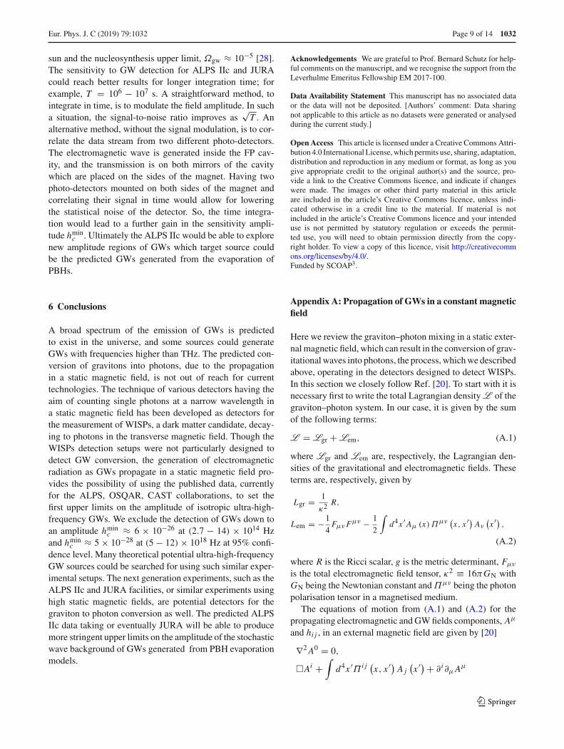
6 Conclusions

A broad spectrum of the emission of GWs is predictedto exist in the universe, and some sources could generateGWs with frequencies higher than THz. The predicted con-version of gravitons into photons, due to the propagationin a static magnetic field, is not out of reach for currenttechnologies. The technique of various detectors having theaim of counting single photons at a narrow wavelength ina static magnetic field has been developed as detectors forthe measurement of WISPs, a dark matter candidate, decay-ing to photons in the transverse magnetic field. Though theWISPs detection setups were not particularly designed todetect GW conversion, the generation of electromagneticradiation as GWs propagate in a static magnetic field pro-vides the possibility of using the published data, currentlyfor the ALPS, OSQAR, CAST collaborations, to set thefirst upper limits on the amplitude of isotropic ultra-high-frequency GWs. We exclude the detection of GWs down toan amplitude hmin

c ≈ 6 × 10−26 at (2.7 − 14) × 1014 Hzand hmin

c ≈ 5 × 10−28 at (5 − 12) × 1018 Hz at 95% confi-dence level. Many theoretical potential ultra-high-frequencyGW sources could be searched for using such similar exper-imental setups. The next generation experiments, such as theALPS IIc and JURA facilities, or similar experiments usinghigh static magnetic fields, are potential detectors for thegraviton to photon conversion as well. The predicted ALPSIIc data taking or eventually JURA will be able to producemore stringent upper limits on the amplitude of the stochasticwave background of GWs generated from PBH evaporationmodels.

Acknowledgements We are grateful to Prof. Bernard Schutz for help-ful comments on the manuscript, and we recognise the support from theLeverhulme Emeritus Fellowship EM 2017-100.

Data Availability Statement This manuscript has no associated dataor the data will not be deposited. [Authors’ comment: Data sharingnot applicable to this article as no datasets were generated or analysedduring the current study.]

Open Access This article is licensed under a Creative Commons Attri-bution 4.0 International License, which permits use, sharing, adaptation,distribution and reproduction in any medium or format, as long as yougive appropriate credit to the original author(s) and the source, pro-vide a link to the Creative Commons licence, and indicate if changeswere made. The images or other third party material in this articleare included in the article’s Creative Commons licence, unless indi-cated otherwise in a credit line to the material. If material is notincluded in the article’s Creative Commons licence and your intendeduse is not permitted by statutory regulation or exceeds the permit-ted use, you will need to obtain permission directly from the copy-right holder. To view a copy of this licence, visit http://creativecommons.org/licenses/by/4.0/.Funded by SCOAP3.

Appendix A: Propagation of GWs in a constant magneticfield

Here we review the graviton–photon mixing in a static exter-nal magnetic field, which can result in the conversion of grav-itational waves into photons, the process, which we describedabove, operating in the detectors designed to detect WISPs.In this section we closely follow Ref. [20]. To start with it isnecessary first to write the total Lagrangian density L of thegraviton–photon system. In our case, it is given by the sumof the following terms:

L = Lgr + Lem, (A.1)

where Lgr and Lem are, respectively, the Lagrangian den-sities of the gravitational and electromagnetic fields. Theseterms are, respectively, given by

Lgr = 1

κ2 R,

Lem = −1

4FμνF

μν − 1

2

∫d4x ′Aμ (x)Πμν

(x, x ′) Aν

(x ′) ,

(A.2)

where R is the Ricci scalar, g is the metric determinant, Fμν

is the total electromagnetic field tensor, κ2 ≡ 16πGN withGN being the Newtonian constant and Πμν being the photonpolarisation tensor in a magnetised medium.

The equations of motion from (A.1) and (A.2) for thepropagating electromagnetic and GW fields components, Aμ

and hi j , in an external magnetic field are given by [20]

∇2A0 = 0,

�Ai +∫

d4x ′Π i j (x, x ′) A j(x ′) + ∂ i∂μA

μ

123

1032 Page 10 of 14 Eur. Phys. J. C (2019) 79 :1032

= κ ∂μ[hμβ F iβ − hiβ Fμ

β ],�hi j = −κ

(Bi B j + Bi B j + Bi B j

), (A.3)

where Aμ = (φ, A) is the incident electromagneticvector-potential with magnetic field components Bi and Biare the components of the external magnetic field vector B . Inobtaining the system (A.3) we made use of the TT-gauge con-ditions for the GWs tensor h0μ = 0, hii = 0 and ∂ j hi j = 0.As shown in detail in Ref. [20], the system (A.3) can be lin-earised by making use of the slowly varying envelope approx-imation (SVEA) which is a WKB-like approximation for aslowly varying external magnetic field of spacetime coordi-nates. In this approximation, and for propagation along theobserver’s z axis in a given cartesian coordinate system, Eq.(A.3) can be written as [20]

(ω + i∂z) Ψ(z, ω, z

)I + M (z, ω) Ψ

(z, ω, z

) = 0, (A.4)

where in (A.4) I is the unit matrix,Ψ(z, ω, z

)= (h×, h+, Ax ,

Ay)T is a four component field with h×,+ being the usual

GW cross and plus polarisation states and Ax,y are the usualpropagating transverse photon states. In (A.4) M (z, ω) is themass mixing matrix, which is given by

M (z, ω) =

⎛

⎜⎜⎝

0 0 −iMxgγ iM y

gγ

0 0 iM ygγ iMx

gγiMx

gγ −iM ygγ Mx MCF

−iM ygγ −iMx

gγ M∗CF My

⎞

⎟⎟⎠ , (A.5)

where the elements of the mass mixing matrix M are givenby

Mxgγ = κ k Bx/ (ω + k) ,

Mygγ = κ k By/ (ω + k) ,

Mx = −Πxx/ (ω + k) ,

My = −Πyy/ (ω + k) ,

MCF = −Πxy/ (ω + k) .

Here MCF is a term which includes a combination of theCotton–Mouton and Faraday effects in a plasma and whichdepends on the magnetic field direction with respect to thephoton propagation. Here ω is the total energy of the fields,namely ω = ωgr = ωγ . In this work all the particles partic-ipating in the mixing are assumed to be relativistic, namelyω + k � 2k with k being the magnitude of the photon andgraviton wave-vectors.

The system of differential equations (A.4) does not haveclosed solutions in the case when the mixing occurs in arbi-trary matter that evolves in space and time, namely in the casewhen the system of differential equations is with variablecoefficients such as in cosmological scenarios. However, inthe case of mixing in a laboratory magnetic field, the system(A.4) can be simplified by considering a specific propaga-tion of GWs with respect to the magnetic field direction and

by considering the propagation in the magnetic field withoutgas or a plasma present (see below). For example, first onecan choose the magnetic field to be transverse to the photondirection of propagation such as B = (

Bx , 0, 0)

where wehave My

gγ = 0 and MCF = 0. Second, if there is a gas ora plasma in addition to the external magnetic field, usuallywe have Mx �= My , which essentially means that the trans-verse photon states have different indices of refraction. Inthe case when one is able to achieve almost a pure vacuumin the laboratory, the contribution of the gas or plasma tothe index of refraction can be safely neglected while there isalso still present a contribution to the index of refraction dueto the vacuum polarisation in the magnetic field. However,the latter contribution is completely negligible because themagnitude of the laboratory magnetic field is usually a few Tand consequently is too small to have any appreciable effecton Mx and My .

As discussed above, let us consider first the case when theexternal magnetic field is completely transverse with respectto the photon direction of propagation where My

gγ = 0 andMCF = 0. The fact that MCF = 0 is because By = 0, Bz = 0and consequently the term corresponding to the Faradayeffect is absent since this effect occurs only when the mag-netic field has a longitudinal component along the electro-magnetic wave direction of propagation. In addition, in theMCF term the term corresponding to the Cotton–Moutoneffect in plasma also is zero because by convention we havechosen By = 0. After these considerations several termsin the mixing matrix M (z, ω) are zero and in the case ofthe medium in the laboratory being homogeneous in space(including the magnetic field), the mass mixing matrix Mdoes not depend on the coordinate z. In this case the commu-tator [M (z, ω) , M

(z′, ω

)] = 0 and the solution of the sys-tem (A.4) is given by taking the exponential of M (z, ω). Con-sequently, we obtain the following solutions for the fields:

h×(z, ω, z

) =[

cos (Δx z) − iMx sin (Δx z)

2Δx

]ei(ω+ Mx

2

)zh×

(0, ω, z

)

+ Mxgγ sin (Δx z)

Δxei(ω+Mx /2)z Ax

(0, ω, z

),

h+(z, ω, z

) =[

cos(Δy z

) − iMy sin

(Δy z

)

2Δy

]

ei(ω+ My

2

)zh+

(0, ω, z

)

− Mxgγ sin

(Δy z

)

Δyei(ω+My/2)z Ay

(0, ω, z

),

Ax(z, ω, z

) = − Mxgγ sin (Δx z)

Δxei(ω+ Mx

2

)zh×

(0, ω, z

)

+[

cos (Δx z) + iMx sin (Δx z)

2Δx

]ei(ω+Mx /2)z Ax

(0, ω, z

),

Ay(z, ω, z

) = Mxgγ sin

(Δy z

)

Δyei(ω+ My

2

)zh+

(0, ω, z

)

+[

cos(Δy z

) + iMy sin

(Δy z

)

2Δy

]

ei(ω+ My

2

)zAy

(0, ω, z

),

(A.6)

123

Eur. Phys. J. C (2019) 79 :1032 Page 11 of 14 1032

where h×,+(0, ω, z

)and Ax,y

(0, ω, z

)are, respectively,

the GW and electromagnetic wave initial amplitudes at theorigin of the coordinate system z = 0, namely the amplitudesbefore entering the region where the magnetic field is located.In addition, we have defined

Δx,y ≡

√

M2x,y + 4

(Mx

gγ

)2

2. (A.7)

Appendix B: Electromagnetic energy fluxes generatedwith laboratory graviton–photon mixing

In the previous appendix we found the solutions of the lin-earised equations of motion (A.4) for the GW fields h×,+ andfor the electromagnetic wave fields Ax,y . In this section weuse these solutions to find the energy flux of the electromag-netic radiation generated in the laboratory for the graviton–photon mixing (in equations abbreviated as graph). Beforeproceeding further is important to stress that in (A.6), theGW amplitudes h×,+ are not dimensionless, as they are com-monly defined in some textbooks, but have energy dimensionunits. This is due to the fact that in Ref. [20] the metric ten-sor is expanded as gμν = ημν + κhμν where the GW tensorhμν has the physical dimensions of an energy. But in manycases one also writes gμν = ημν + hμν where in this casehμν is a dimensionless quantity. Since the latter case is quitecommon in the theory of GWs and because we want to con-form to the literature, in Eq. (A.6) one has to simply replaceh×,+ (0, t) = h×,+ (0, t) /κ , where h×,+ are now dimen-sionless amplitudes.

Consider the case when GWs enter a region of constantexternal magnetic field in the laboratory and that initiallythere are no electromagnetic waves.

The assumption of no initial electromagnetic waves meansthat Ax

(0, ω, z

) = Ay(0, ω, z

) = 0 in the solutions (A.6).Therefore, the expressions for the electromagnetic field com-ponents, in the graviton to photon mixing for a transversepropagation with respect to the magnetic field, are given by

Ax(z, ω, z

) = −Mxgγ sin (Δx z)

κΔxei(ω+Mx/2)z h×

(0, ω, z

),

Ay(z, ω, z

) = Mxgγ sin

(Δyz

)

κΔyei(ω+My/2)z h+

(0, ω, z

).

(B.8)

The expressions for the electromagnetic field componentsin (B.8), even though very important, are not very useful forpractical purposes since we usually detect electromagneticradiations through the energy transported to the detector. Forthis reason it is better to work with the Stokes parameterIγ (z, t) ≡ Φγ (z, t) of the electromagnetic radiation gener-ated in the graviton to photon mixing and which quantifies theenergy flux (or energy density) of the electromagnetic radi-

ation. The Stokes parameter Φγ , at a given point in space z,is defined as

Φγ (z, t) ≡ 〈|Ex (z, t) |2〉 + 〈|Ey (z, t) |2〉, (B.9)

where Ex and Ey are the components of the electric fieldof electromagnetic radiation and the symbol 〈(·)〉 denotestemporal average of quantities over many oscillation periodsof electromagnetic radiation. The components of the electricfield E are related to that of the vector-potential A throughthe relation Ex,y (z, t) = −∇A0 (z, t) − ∂t Ax,y (z, t). For aglobally neutral medium (if there is one except the magneticfield) in the laboratory we can choose A0 = 0 from thefirst equation in (A.3) and then we simply get Ex,y (z, t) =−∂t Ax,y (z, t).

In order to calculate the energy density of the electro-magnetic radiation and related quantities in the graviton tophoton mixing, we need first to make some assumptions onthe GW signal which interacts with the magnetic field in thelaboratory. In this work we concentrate on our study on astochastic background of GWs with astrophysical or cosmo-logical origin. It is rather natural to assume that the stochasticbackground of GWs is isotropic, unpolarised and stationary[28,32]. In order to make more clear what these assumptionsmean, we write the GW amplitude tensor hi j (z, t) at z = 0as a Fourier integral

hi j (0, t) =∑

λ=×,+

∫ +∞

−∞dω

2π

∫

S2d2n hλ

(0, ω, n

)eλi j

(n)e−iωt ,

(i, j = x, y, z) , (B.10)

where n is a unit vector on the two sphere S2, whichdenotes an arbitrary direction of propagation of the GW,d2n = d (cos θ) dφ, λ is the polarisation index of theGW with the usual cross and plus polarisation states andeλi j

(n)

is the GW polarisation tensor, which has the property

eλi j

(n)ei jλ′

(n) = 2δλλ′ . The assumptions that the stochastic

background is isotropic, unpolarised and stationary meansthat the ensemble average of the Fourier amplitudes satisfies

〈hλ

(0, ω, n

)h∗

λ′(0, ω′, n′)〉 = 2πδ

(ω − ω′) δ2

(n, n′)

4πδλλ′

×H (0, ω)

2, (B.11)

where H (0, ω) is defined as the spectral density of thestochastic background of GW and it has the physical dimen-sions of Hz−1 and δ2

(n, n′) = δ

(φ − φ′) δ

(cos θ − cos θ ′)

is the covariant Delta function on the two sphere. One cancheck by using (B.10) and (B.11) that the ensemble average〈hi j (0, t) hi j (0, t)〉, is given by

123

1032 Page 12 of 14 Eur. Phys. J. C (2019) 79 :1032

〈hi j (0, t) hi j (0, t)〉 = 2∫ +∞

−∞dω

2πH (0, ω) (B.12)

= 4∫ +∞

0

d (log ω)

2πω H (0, ω)

≡ 2∫ +∞

0d (log ω) h2

c (0, ω) , (B.13)

where the last equality in (B.12) defines the characteristicamplitude, hc (dimensionless), of a stochastic backgroundof GWs. In obtaining (B.12) we used the fact that for anunpolarised stochastic background, we have, on average,〈|h× (0, ω) |2〉 = 〈|h+ (0, ω) |2〉 �= 0, while the ensembleaverage of the mixed terms vanishes identically. We mayobserve that by comparing the two last equalities in (B.12)we get h2

c (0, ω) = 2ωH (0, ω) / (2π).With Eqs. (B.10)–(B.12) at hand we are in a position to

calculate Φγ and relate it with hc or H . Let us at this pointwrite the components of the vector-potential for n = z asFourier integrals,

Ax,y (z, t) =∫ +∞

−∞dω

2π

∫d2 z Ax,y

(z, ω, z

)e−iωt .

(B.14)

Then by using Eq. (B.14) in Ex,y (z, t) = −∂t Ax,y (z, t)and then putting all results together in the expression of theStokes parameter (B.9), we get

Φγ (z, t) =(Mx

gγ

)2∫ +∞

0

dω

2π

[sin2 (Δx z)

Δ2x

+ sin2(Δy z

)

Δ2y

]

ω2H (0, ω)

κ2 , (B.15)

where in obtaining Eq. (B.15) we used also Eq. (B.11). Inaddition, we may note that both Δx and Δy implicitly dependon ω through Mx and My and thus explain the reason whyΔx,y do appear under the integral sign in (B.15). On the otherhand, Mx

gγ does not depend on ω since we are consideringrelativistic particles with ω � k.

Now in order to relate the total energy density of theformed electromagnetic radiation in the graviton–photonmixing, we may note from Eq. (B.15) that the energy densitycontained in a logarithmic energy interval, is given by

dΦgraphγ (z, ω; t)d (log ω)

=(Mx

gγ

)2[

sin2 (Δx z)

Δ2x

+ sin2(Δyz

)

Δ2y

]ω3H (0, ω)

2πκ2

=(Mx

gγ

)2

2

[sin2 (Δx z)

Δ2x

+ sin2(Δyz

)

Δ2y

]ω2h2

c (0, ω)

κ2 .

(B.16)

The expression dΦgraphγ (z, ω; t) /d (log ω) in (B.16) tells us

how much of the total energy density is contained in a loga-rithmic energy interval. Equation (B.16) can be written alsoin an equivalent form in terms of the density parameter ofphotons Ωγ and the density parameter of GWs, Ωgw. Thedensity parameter of a species i of particles at the energy ω

is defined as

Ωi (z, ω; t) ≡ 1

ρc

dρi (z, ω; t)d (log ω)

, (B.17)

where ρc is the critical energy density to close the universe,ρc = 6H2

0 /κ2, where H0 is the Hubble parameter H0 =100 h0 (km/s/Mpc) with h0 being a dimensionless parameterwhich is determined experimentally. In addition since theenergy density (or energy flux Φ) of GWs is given by

ρgw (0, t) = 〈hi j (0, t) hi j (0, t)〉2κ2

=∫ +∞

0d (log ω)

ω2h2c (ω)

κ2 , (B.18)

where we used (B.10)–(B.11), we have from (B.16), (B.17)and (B.18)

h20Ω

graphγ (z, ω; t) =

(Mx

gγ

)2

2

[sin2 (Δx z)

Δ2x

+ sin2(Δyz

)

Δ2y

]

×h20Ωgw (0, ω; t) . (B.19)

Equations (B.16) and (B.19) essentially give a completedescription of how the graviton to photon mixing propagatesin space in a transverse and constant magnetic field anduniform medium. Equations (B.16) and (B.19) are equallyimportant and can be used in different contexts in order tocompare with experimental data. It is very important to anal-yse these expressions in some limiting cases. Consider thecase when in the laboratory there is a medium (gas or plasma)in addition to the magnetic field and when Mx = My . The lastcondition essentially means that the two propagating trans-verse states of the electromagnetic radiation have the sameindex of refraction. When Mx = My , we have Δx = Δy andconsequently we get for (B.19)

h20Ω

graphγ (z, ω) =

(Mx

gγ

)2[

sin2 (Δx z)

Δ2x

]h2

0Ωgw (0, ω) .

(B.20)

Another important situation is when in the laboratory thereis not a medium but only a magnetic field in vacuum. In thiscase we have Δx = Δy = Mx

gγ and the graviton–photonmixing is maximal or resonant

h20Ω

graphγ (z, ω) = [sin2

(Mx

gγ z)]h2

0Ωgw (0, ω) . (B.21)

Equation (B.21) tells us that the graviton–photon mixingshows an oscillatory behaviour with the distance z in the max-

123

Eur. Phys. J. C (2019) 79 :1032 Page 13 of 14 1032

imum mixing case. For a long distance of travelling, there are

values of z which make sin2(Mx

gγ z)

= 1 and in that case

we see that all GWs are transformed into electromagneticwaves. However, since Mx

gγ is usually a very small quantity,one needs huge distances of travelling in order to meet withthis situation. In many practical cases we have Mx

gγ z � 1

and we can approximate sin2(Mx

gγ z)

�(Mx

gγ z)2

in the

maximum mixing case.

References

1. B.P. Abbott et al. (LIGO Scientific Collaboration and Virgo Col-laboration), Observation of gravitational waves from a binary blackhole merger. Phys. Rev. Lett. 116, 061102 (2016)

2. B.P. Abbott et al. (LIGO Scientific Collaboration and Virgo Col-laboration), GW170817: observation of gravitational waves froma binary neutron star Inspiral. Phys. Rev. Lett. 119, 161101 (2017)

3. D.V. Martynov et al. (LIGO Scientific Collaboration), Compositeoperator and condensate in the SU (N ) Yang–Mills theory withU (N−1) stability group. Phys. Rev. D 93, 112004 (2016) (erratumPhys. Rev. D 97, 059901, 2018)

4. F. Acernese et al. (Virgo Collaboration), Advanced Virgo: a second-generation interferometric gravitational wave detector. Class.Quantum Gravity 32, 2 (2015)

5. K.L. Dooley et al. (GEO 600 Collaboration), GEO 600 and theGEO-HF upgrade program: successes and challenges. Class. Quan-tum Gravity 33, 075009 (2016)

6. K. Somiya (KAGRA collaboration), Detector configuration ofKAGRA—the Japanese cryogenic gravitational-wave detector.Class. Quantum Gravity 29, 124007 (2012)

7. S. Vitale, Space-borne gravitational wave observatories. Gen. Rel-ativ. Gravit. 46, 1730 (2014)

8. Pau Amaro-Seoane et al., Laser Interferometer Space Antenna(LISA). arXiv:1702.00786v3 [astroph.IM] (2017)

9. G. Hobbs et al. (IPTA Collaboration), The international pulsar tim-ing array project: using pulsars as a gravitational wave detector.Class. Quantum Gravity 27, 27 (2010)

10. M. Kramer, D.J. Champion, The European pulsar timing array andthe large European array for pulsars. Class. Quantum Gravity 30,22 (2013)

11. P.B. Demorest et al. (NanoGrav Collaboration), Limits on thestochastic gravitational wave background from the North Amer-ican nanohertz observatory for gravitational waves. Astrophys. J.762, 94 (2013)

12. D. Boccaletti, Conversion of photons into gravitons and vice versain a static electromagnetic field. Nuovo Cimento 70(B), 129 (1970)

13. Y.B. Zeldovich, Electromagnetic and gravitational waves in a sta-tionary magnetic field. Sov. Phys. JETP 65, 1311 (1973)

14. W.K. De Logi, A.R. Mickelson, Electrogravitational conversioncross sections in static electromagnetic fields. Phys. Rev. D 16,2915 (1977)

15. G. Raffelt, L. Stodolsky, Mixing with photo with low-mass parti-cles. Phys. Rev. D 37, 1237 (1988)

16. P.G. Macedo, A.H. Nelson, Propagation of gravitational waves ina magnetized plasma. Phys. Rev. D 28, 2382 (1983)

17. D. Fargion, Prompt and delayed radio bangs at kilohertz by SN1987A: a test for graviton–photon conversion. Gravit. Cosmol. 1,301 (1995)

18. A.M. Cruise, The potential for very high-frequency gravitationalwave detection. Class. Quantum Gravity 29, 9 (2012)

19. A.D. Dolgov, D. Ejlli, Conversion of relic gravitational waves intophotons in cosmological magnetic fields. JCAP 1212, 003 (2012).arXiv:1211.0500 [gr-qc]

20. D. Ejlli, V.R. Thandlam, Graviton–photon mixing. Phys. Rev. D99, 044022 (2019)

21. M.E. Gertsenshtein, Wave resonance of light and gravitationalwaves. Sov. Phys. JETP 14, 84 (1962)

22. G.A. Lupanov, A capacitor in the field of a gravitational wave.JETP 25, 76 (1967)

23. F. Bastianelli, C. Schubert, One loop photon–graviton mixing inan electromagnetic field: part 1. J. High Energy Phys. 0502, 069(2005)

24. F. Bastianelli, U. Nucamendi, C. Schubert, V.M. Villanueva, Oneloop photon–graviton mixing in an electromagnetic field: part 2. J.High Energy Phys. 0711, 099 (2007)

25. W.-T. Ni, One hundred years of general relativity: from genesisand empirical foundations to gravitational waves, cosmology andquantum gravity. World Sci. (Singapore) 1, 461–464 (2016)

26. G.S. Bisnovatyi-Kogan, V.N. Rudekno, Very high frequency gravi-tational wave background in the universe. Class. Quantum Gravity21, 3347 (2004)

27. L.P. Grishchuk, Primordial gravitons and possibility of their obser-vation. JEPT Lett. 23, 293 (1976)

28. M. Maggiore, Gravitational wave experiments and early universecosmology. Phys. Rep. 331, 283 (2000). arXiv:gr-qc/9909001

29. C. Clarkson, S.S. Seahra, A gravitational wave window on extradimensions. Class. Quantum Gravity 24, F33 (2007)

30. M. Servin, G. Brodin, Resonant interaction between gravitationalwaves, electromagnetic waves, and plasma flows. Phys. Rev. D 68,044017 (2003)

31. B. Allen, in Relativistic Gravitation and Gravitational Radiation,ed. by J.A. Marck, J.P. Lasota (Cambridge University Press, Cam-bridge, 1997), p. 373

32. B. Allen, J.D. Romano, Detecting a stochastic background of grav-itational radiation: signal processing strategies and sensitivities.Phys. Rev. D 59, 102001 (1999). arXiv:gr-qc/9710117

33. L.P. Grishchuk, Electromagnetic generators and detectors of grav-itational waves. arXiv:gr-qc/0306013 (2003)

34. T. Nakamura, M. Sasaki, T. Tanaka, Kip S. Thorne, Gravitationalwaves from coalescing black hole MACHO binaries. Astro. Phys.J. 487, L139–L142 (1997)

35. D. Alexander, Damian Ejlli, Relic gravitational waves from lightprimordial black holes. Phys. Rev. D 84, 024028 (2011)

36. V. Anastassopoulos et al. (CAST Collaboration), New CAST limiton the axion–photon interaction. Nat. Phys. 13, 584–590 (2017)

37. V.B. Braginskii, V.N. Rudenko, Sci. Notes Kazan Univ. v.123 12,96–108 (1963)

38. D.V. Galtsov, YuV Gratz, Gravitational radiation during Coulombcollisions. Sov. Phys. J. 17(12), 94–99 (1974)

39. S. Weinberg (ed.) Gravitation and Cosmology. Wiley, New York,p. 266 (1972)

40. A.M. Cruise, R.M.J. Ingley, A prototype gravitational wave detec-tor for 100 MHz. Class. Quantum Gravity 23, 22 (2006)

41. T. Akutsu et al., Search for a stochastic background of 100-MHzgravitational waves with laser interferometers. Phys. Rev. Lett. 101,101101 (2008)

42. A. Nishizawa et al., Laser-interferometric detectors for gravita-tional wave backgrounds at 100 MHz: detector design and sensi-tivity. Phys. Rev. D 77, 022002 (2008)

43. A.S. Chou et al., (Holometer Collaboration) MHz gravitationalwave constraints with decameter Michelson interferometers. Phys.Rev. D 95, 063002 (2017)

44. A. Ito, T. Ikeda, K. Miuchi, J. Soda, Probing GHz gravitationalwaves with graviton–magnon resonance. arXiv:1903.04843v2(2019)

123

1032 Page 14 of 14 Eur. Phys. J. C (2019) 79 :1032

45. K. Ehret et al. (ALPS collaboration), New ALPS results on hidden-sector lightweights. Phys. Lett. B 689, 149–155 (2010)

46. R. Ballou, G. Deferne, M. Finger Jr., M. Finger, L. Flekova, J.Hosek, S. Kunc, K. Macuchova, K.A. Meissner et al. (OSQARcollaboration), New exclusion limits on scalar and pseudoscalaraxionlike particles from light shining through a wall. Phys. Rev. D92, 092002 (2015)

47. ALPS I Collaboration, K. Ehret et al., Nucl. Instrum. Methods A612, 83–96 (2009). arXiv:0905.4159

48. P. Pugnat et al. (OSQAR collaboration), Search for weakly inter-acting sub-eV particles with the OSQAR laser-based experiment:results and perspectives. Eur. Phys. J. C 74, 3027 (2014)

49. G.G. Javier, Micromegas for the search of solar axions in CAST andlow-mass WIMPs in TREX-DM. PhD Thesis, University Zaragoza,p. 99 (2015)

50. R. Bahre, B. Dobrich, J. Dreyling-Eschweiler, S. Ghazaryan, R.Hodajerdi, D. Horns, F. Januschek, E.A. Knabbe, A. Lindner, D.Notz, A. Ringwald, J.E. von Seggern, R. Stromhagen, D. Trines,B. Willke, Any light particle search II Technical Design Report.Rep. J. Instrum. 8, T09001 (2013)

51. J. Beacham et al, Physics beyond colliders at CERN:beyond the standard model working group report: laboratoryexperiments: CERN-PBC-REPORT-2018-007 (JURA), p. 21.arXiv:1901.09966v2 (2018)

52. J. Dreyling-Eschweiler, A superconducting microcalorimeter forlow-flux detection of near-infrared single photons. PhD Thesis,Department Physik, der Universität Hamburg, p. 168 (2014)

53. E. Armengaud et al., Conceptual design of the International AxionObservatory (IAXO). Jinst 9, T05002 (2014)

54. P. Sikivie, D.B. Tanner, Karl van Bibber, Resonantly enhancedaxion–photon regeneration. Phys. Rev. L 98, 172002 (2007)

55. N.I. Kolosnitsyn, V.N. Rudenko, Gravitational Hertz experimentwith electromagnetic radiation in a strong magnetic field. Phys.Scr. 90, 074059 (2015)

56. A.E. Siegman, Lasers (University Science Books), Ch. 11.3, pp.413–428 (1986)

57. N. Ismail, Cristine C. Kores, D. Geskus, M. Pollnau, Fabry–Pérotresonator: spectral line shapes, generic and related airy distribu-tions, linewidths, finesses, and performance at low or frequency-dependent reflectivity. Opt. Express 24, 15 (2016)

58. S.W. Hawking, Black holes and thermodynamics. Phys. Rev. D 13,191–197 (1976)

59. Don N. Page, Particle emission rates from a black hole: masslessparticles from an uncharged, nonrotating hole. Phys. Rev. D 13,198 (1976)

123