1

Updates to OPGEE

OPGEE v3.0a candidate model

Adam R. Brandt, Mohammad S. Masnadi, Jeff Rutherford, Jacob Englander

Energy Resources Engineering Department, Stanford University

CARB OPGEE Modeling update

California Air Resources Board

October 14th, 2020

1

22

Outline

Part 1: Background and context

Part 2: Updates to the OPGEE model

› Improving stream tracking

› Gas processing simulation with process simulators

› Gas fugitives modeling with improved datasets and

statistical modeling

› Gas functional unit allowed for primarily gas fields

Masnadi et al., Science, 361 (6405), 851-853.

3

Part 1: Background and context

4

OPGEE model

Source: El-Houjeiri and Brandt (2012a, 2012b)

• Model is called Oil Production Greenhouse gas Emissions

Estimator (OPGEE)

• Estimates emissions given field parameters and technologies

The first open-source GHGtool for oil and gas operations• Anyone can download, modify and use• 36 published papers, complete

documentation (~400 pp.) with all sources defined

• Funded by CARB, U.S. DOE, Carnegie Endowment, Ford Motor Co., Saudi Aramco

5

OPGEE model timeline

• Model development started in 2010

• First official version: OPGEE v1.0 released September 2012

• Second official version: OPGEE v2.0 released Feb 2018

• Third official version (candidate): OPGEE v3.0a - Introduced today

• Bibliography at end of slides:

Used in studies of crude oil CI for • US (Cooney et al. 2017, Yeh et al

2017, Brandt et al. 2016)• Canada (Cai et al. 2015,

Englander et al. 2015)• China (Masnadi et al. 2018a)• Globe (Masnadi et al. 2018b)

Methods development• Overall (El-Houjeri et al. 2013)• Drilling (Vafi et al. 2016)• Gas processing (Masnadi et al.

2020• Uncertainty (Vafi et al. 2014a,

2014b, Brandt et al. 2015)• Time trends (Masnadi et al.

2018c, Tripathi et al. 2017)

6

Part 2: Updates to the model

7

Challenge 1: Model organization and stream tracking

• OPGEE v2.0 had drawbacks in model organization and stream

tracking

• Gas balance sheet tracked gas species, but other streams were not

reliably tracked

• Process units were not on individual sheets, and unclear exactly which

mass flows were entering and leaving each sheet

• Pressures and other properties of streams not reliably tracked

• No easy way to navigate along the processing path

• OPGEE v3.0a includes a completely reworked model “skeleton”

• All streams of oil, water, gas, etc. are tracked in mass flows

• Conservation of mass ensured at process unit and total model level

• Pressures, temperatures, and other properties tracked

• Navigation aided by graphical view of process connections (PFD)

88

Improvement: OPGEE 3.0 process flow sheet map

Production site boundary

Post-transport and storage Post distribution

Streams differentiated by colorGreen – OilRed – GasBlue – WaterYellow – ElectricityPurple – Other gasBlack – Raw bitumen

99

Graphical navigation

Trace flows along processing paths and click to navigate to sheets

Mass flows into and out of each process unit tracked

1010

Flow sheet

Mass flows

Properties

Stream number

1111

Mass balance tracking and error flagging

Errors easier to spot with mass balancetracking across entire model

1212

Field

Transport

Gas as a primary product, different assessment points

OPGEE 2.0 always required oil to

be the primary product

CI: gCO2/MJ oil at refinery inlet

OPGEE 3.0 allows for gas as the

primary product

CI: gCO2/MJ gas at transportation

system inlet

Oil at field boundary or refinery inlet

Gas at field boundary, transportation inlet or consumer

13

Challenge 2: Gas processing simulation

• OPGEE v2.0 had relied on ”textbook” treatment of gas processing units

• Models largely taken from classic text Manning and Thompson

• Simple models of energy use and power requirements per unit of throughput

• No way to customize process unit energy use for particular conditions

• Feedback from industry: “Why not use process simulation tools?”

• OPGEE v3.0a includes ”proxy” models generated from process simulation tools

• Obtained access to Aspen HYSYS process simulation package

• Work from template models of 4 key gas processing units

• Acid Gas Removal, Dehydration, Demethanizer, Claus Unit

• Simulated many cases at a variety of conditions

• Generated statistical representations to predict Aspen HYSYS results

M.S. Masnadi *, P.R. Perrier , J. Wang , J. Rutherford , A.R. Brandt.

Statistical proxy modeling for life cycle assessment and energetic analysis.

Energy DOI: 10.1016/j.energy.2019.116882

1414

Example: AGR modeling using process simulation software

Modeled AGR unit in Aspen HYSYS chemical process simulation

Five different solvents (amines):

› 1. MEA; 2. DEA (30% wt.); 3. DEA high load (35% wt.); 4. MDEA; 5. DGA

Five independent variables:

› 1. CO2 concentration; 2. H2S concentration; 3. Regeneration reflux ratio; 4.

Regeneration feed temperature; 5. Acid gas pressure

1515

Sampling approaches

AGR input variables to be sampled:

CO2 concentration in gas

H2S concentration in gas

Reflux ratio

Regenerator feed temperature

Feed gas pressure

Deterministic sampling:

Box-Behnken

Random sampling:

Latin hypercube

Total of ∼9000 simulations of AGR systems across independent variables

1616

Proxy modeling (cont’d)

Experimental design: five independent variables

› Settings of each dependent on type of solvent applied

› Model is allowed to adjust some parameters to make simulation converge

(e.g., amine circulation rate)

› Save combination of 5 input variables plus multiple outputs

1717

Training and testing dataset

After 9,000 simulations, dataset is

split into training and testing

Training data used to fit optimal

model functional form

Test data “held out” and never

examined until reporting results

Tested variety of polynomial and

other classical models

Quadratic regression balances

complexity and fit

Total dataset

Training data

Test data

90% training10% testing

1818

Test fitted AGR model against hold-out set

Reboiler

Pump

Condenser

Cooler

1919

Demethanizer product composition results

Composition and shares of C1, C2, C3 to streams harder to predict

2020

Take-aways from process simulation

• Quadratic regression able to fit

extremely well in most cases

• Most fits have R2 >0.95

• OPGEE now produces, for cases

within our sampled input ranges,

results very close to Aspen

HYSYS

Challenges for extension

Expertise and software license

Computational requirements very

large for 10,000s of simulations

Unable to extrapolate – Can only

model ranges of T, P,

composition sampled

21

Challenge 3: Fugitive and vented CH4 emissions

• OPGEE v2.0 relied on CARB survey data for fugitive and vented CH4

• Survey of California producers required detailed reporting on emissions

• Emissions factors obtained from EPA GHG Inventory

• Survey unable to account for differences between US regions

• Independent measurements lacking, with lots of studies done since OPGEE

v2.0

• OPGEE v3.0a includes modern, independently measured field data for CH4

emissions sources

• Two models: “site” and “component” level

• Component level data draws from multiple studies, 1000s of measured leaks

• Monte Carlo sampling approach includes super-emitter characteristics

• Able to recreate observed US wide emissions (e.g., Alvarez et al. 2018)

J.S. Rutherford, E.D. Sherwin, A.P. Ravikumar, G.A. Heath, J.G. Englander, D. Cooley, D. Lyon, M. Omara, Q. Langfitt, A.R. Brandt Closing the gap: Explaining persistent underestimation by US oil and natural gas production-segment methane inventories Submitted: Nature Energy

2222

Top-down

e.g., Zhang et al. 2020, Permian Basin

Bottom-up

Component-level Site-level

e.g., Alvarez et al. 2018, National estimate

e.g., EPA Greenhouse Gas Inventory

Policy and programs Validation and assessment

Different varieties of methane measurement inform our understanding of emissions quantities and sources

2323

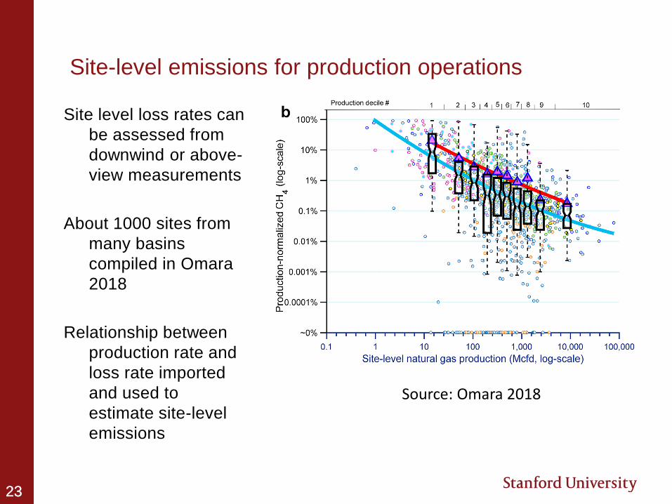
Site-level emissions for production operations

Site level loss rates can

be assessed from

downwind or above-

view measurements

About 1000 sites from

many basins

compiled in Omara

2018

Relationship between

production rate and

loss rate imported

and used to

estimate site-level

emissions

Source: Omara 2018

2424

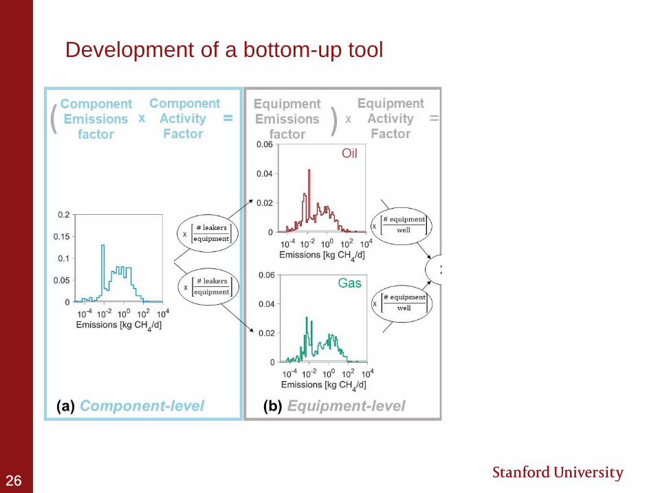
Collecting component-level data from various studies

• Informed by comprehensive literature search of

component-level surveys (6 studies, ~3200

measurements)

• Filtered to (in current OPGEE version) include US studies

only

• Limited global coverage

• Future model versions could include emissions

distributions from other regions

• Data consolidated to consistent component and equipment

type categories

• Consistent component definitions (details in full paper)

allow combination of samples from different studies

• Consistent equipment definitions allows generation of

component counts per equipment

2525

Development of a bottom-up tool

2626

Development of a bottom-up tool

2727

Development of a bottom-up tool

2828

Fraction loss rates: Oil wells (<100 mscf/bbl)

Results of loss fraction are strong

function of well productivity

This effect has been seen repeatedly in

the empirical literature

2929

Using equipment distributions in OPGEE

• A separate equipment-level loss fraction distribution is generated for

each productivity tranche

• A stochastic leak process will tend to cause higher loss fraction in

less productive wells, even if that well is same age or has similar

equipment type

• Resulting equipment distributions can be used in two ways in OPGEE

1. Deterministic: Create average equipment leakage rate for a given

productivity tranche

2. Uncertainty: Draw a given number of equipment realizations for the

size of the population you are analyzing, randomized from the

sampled equipment types

3030

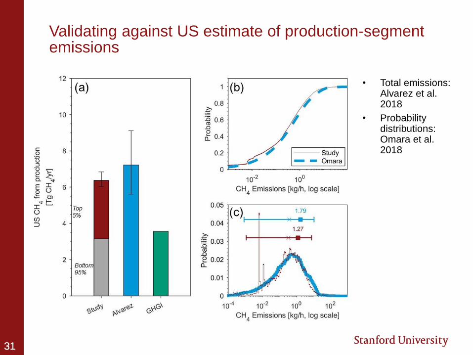
Validating the method

Ideally the method adopted in OPGEE would recreate the key results of

the literature on methane emissions from the last 5 years

Key empirical features that have been found repeatedly that any tool

should be able to show:

1. Larger emissions than classical EPA Greenhouse Gas Inventory

methods

2. Strong dependence of loss fraction on site productivity

3. Strong “heavy-tailed” behavior of emissions distributions: dependence on

large emitters to drive large fraction of emissions

3131

• Total emissions: Alvarez et al. 2018

• Probability distributions: Omara et al. 2018

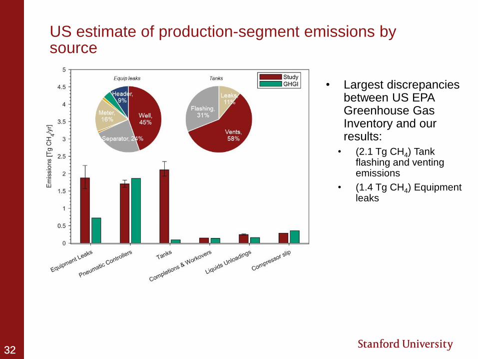
Validating against US estimate of production-segment emissions

3232

• Largest discrepancies between US EPA Greenhouse Gas Inventory and our results:

• (2.1 Tg CH4) Tank flashing and venting emissions

• (1.4 Tg CH4) Equipment leaks

US estimate of production-segment emissions by source

3333

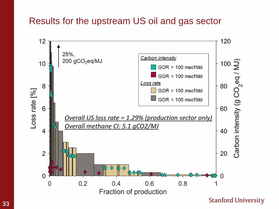
Results for the upstream US oil and gas sector

Overall US loss rate = 1.29% (production sector only)Overall methane CI: 5.1 gCO2/MJ

3434

Bibliography (1)

Jing, L., H.M. El-Houjeiri, J.C. Monfort, A.R. Brandt, M.S. Masnadi, D. Gordon, J.A.

Bergerson. 2020. Carbon intensity of global crude oil refining and mitigation potential.

Nature Climate Change. 11-25. DOI: 10.1111/jiec.12954

M.S. Masnadi *, P.R. Perrier , J. Wang , J. Rutherford , A.R. Brandt. Statistical proxy

modeling for life cycle assessment and energetic analysis. Energy DOI:

10.1016/j.energy.2019.116882

A.R. Brandt. Accuracy of satellite-derived estimates of flaring volume for offshore oil

and gas operations in nine countries. Environmental Research Communications. DOI:

10.1088/2515- 7620/ab8e17.

Nie, Y., S. Zhang, R.E. Liu, D.J. Roda-Stuart, A.P. Ravikumar, A. Bradley, M.S.

Masnadi, A.R. Brandt, J. Bergerson, X. Bi. Greenhouse-gas Emissions of Canadian

Liquefied Natural Gas for Power Generation and District Heating in China: Three

Independent Life Cycle Assessments. Journal of Cleaner Production DOI:

10.1016/j.jclepro.2020.120701

Masnadi, M.S., H.M. El-Houjeiri, D. Schunack, Y. Li, J.G. Englander, A. Badahdah, J.E.

Anderson, T.J. Wallington, J.A. Bergerson, D. Gordon, S. Przesmitzki, I.L. Azevedo, G.

Cooney, J.E. Duffy, G.A. Keoleian, C. McGlade, D.N. Meehan, T.J. Skone, F. You, M.Q.

Wang, A.R. Brandt. Global carbon intensity of crude oil production. Science. DOI:

10.1126/science.aar6859

3535

Bibliography (2)

Brandt, A.R., M.S. Masnadi, J.G. Englander, J.G. Koomey, D. Gordon. Climate-wise

oil choices in a world of oil abundance. Environmental Research Letters DOI:

10.1088/1748- 9326/aaae76

Masnadi, M.S., D. Schunack, Y. Li, S.O. Roberts, A.R. Brandt, H.M. El-Houjeiri, S.

Przesmitzki, M.Q. Wang. Well-to-refinery emissions and net-energy analysis of

China’s crude-oil supply. Na- ture Energy. DOI: 10.1038/s41560-018-0090-7

Yeh, S., A. Ghandi, B.R. Scanlon, A.R. Brandt, H. Cai, M.Q. Wang, Kourosh Vafi,

Robert C. Reedy. Energy intensity and greenhouse gas emissions from oil

production in the Eagle Ford shale. Energy & Fuels DOI:

10.1021/acs.energyfuels.6b02916

Cooney, G., M. Jamieson, J. Marriott, J. Bergerson, A.R. Brandt, T.J. Skone.

Updating the US life cycle GHG petroleum baseline to 2014 with projections to

2014 using open-source engineering-based models. Environmental Science &

Technology DOI: 10.1021/acs.est.6b02819

Masnadi, M.S., A.R. Brandt. Energetic productivity dynamics of global super-giant

oilfields. Energy & Environmental Science. DOI: 10.1039/C7EE01031A

3636

Bibliography (3)

Masnadi, M.S., A.R. Brandt. Climate impacts of oil extraction increase significantly

with oilfield age. Nature Climate Change. DOI: 10.1038/nclimate3347

Tripathi, V. and A.R. Brandt. Estimating decades-long trends in petroleum field energy

re- turn on investment (EROI) with an engineering-based model. PLOS ONE. DOI:

10.1371/jour- nal.pone.0171083

Wang, J., A.R. Brandt, J. O’Donnell. Potential for use of solar energy use in the global

petroleum sector. Energy: The International Journal. DOI:

10.1016/j.energy.2016.10.107

Brandt, A.R., T. Yeskoo, S. McNally, K. Vafi, S. Yeh, H. Cai, M.Q. Wang. Energy

intensity and greenhouse gas emissions from tight oil production in the Bakken

formation. Energy & Fuels. DOI: 10.1021/acs.energyfuels.6b01907

Wallington, T.J., Anderson, J.E., De Kleine, R.D., Kim, H.C., Maas H., Winkler, S.L.,

Brandt, A.R., Keoleian, G.A. (2016). When comparing alternative fuel-vehicle

systems, life cycle as- sessment studies should consider trends in oil production.

Journal of Industrial Ecology. DOI: 10.1111/jiec.12418

Brandt, A.R. (2015). Embodied energy and GHG emissions from material use in

conventional and unconventional oil and gas operations. Environmental Science &

Technology. DOI:10.1021/acs.est.5b03540

3737

Bilbiography (4)

Vafi, K. A.R. Brandt. GHGfrack: A model for estimating greenhouse gas emissions from

drilling vertical and directional wells and hydraulic fracturing. Environmental Science &

Tech- nology. DOI: 10.1021/acs.est.6b01940

Sweeney Smith, S., A. Calbry-Muzyka, A.R. Brandt (2016). Exergetic life cycle

assessment including both inputs and pollutants. International Journal of Life Cycle

Assessment. DOI: 10.1007/s11367-016-1118-5

Kemp, C.E., A.P. Ravikumar, A.R. Brandt (2016) Comparing natural gas leakage detection

technologies using an open-source “virtual gas field” simulator. Environmental Science &

Tech- nology. DOI: 10.1021/acs.est.5b06068

Kang, C.A., Brandt, A.R., Durlofsky, L (2015). A new carbon capture proxy model for opti-

mizing the design and time-varying operation of a coal-natural gas power station.

International Journal of Greenhouse Gas Control. DOI: 10.1016/j.ijggc.2015.11.023

Brandt, A.R., Y. Sun, S. Bharadwaj, D. Livingston, E. Tan, D. Gordon (2015). Energy

return on investment (EROI) for forty global oilfields using a detailed engineering-based

model of oil production. PLOSone. DOI: 10.1371/journal.pone.0144141

3838

Bilbiography (5)

Brandt, A.R., Yeskoo, T.E., K. Vafi. (2015) Net energy analysis of Bakken crude oil

production using a well-level engineering-based model. Energy. DOI:

10.1016/j.energy.2015.10.113

Brandt, A.R., D. Millstein, L. Jin, J.G. Englander (2015). Air quality impacts from well

stimulation. An Independent Scientific Assessment of Well Stimulation in California,

Volume II: Potential Environmental Impacts of Hydraulic Fracturing and Acid

Stimulations. California Council on Science and Technology, Lawrence Berkeley National

Laboratory, July 2015.

Englander, J.G., A.R. Brandt, A. Elgowainy, H. Cai, J. Han, S.L. Yeh, M.Q. Wang (2015).

Oil sands energy intensity assessment using facility-level data. Energy & Fuels.

DOI:10.1021/acs.energyfuels.4b00175

Cai, H., A.R. Brandt, S.L. Yeh, J.G. Englander, J. Han, A. Elgowainy, M.Q. Wang (2015).

Well-to-wheels greenhouse gas emissions of Canadian oil sands products: Implications

for U.S. petroleum fuels. Environmental Science & Technology. DOI:

10.1021/acs.est.5b01255

Brandt, A.R., Y. Sun, K. Vafi (2015). Uncertainty in regional-average petroleum GHG

inten- sities: Countering information gaps with targeted data gathering. Environmental

Science & Technology. 49(1) 679-686. DOI: 10.1021/es505376t

3939

Bibliography (6)

Vafi, K., A.R. Brandt, (2014). Reproducibility of LCA models of crude oil production. Envi-

ronmental Science & Technology. 48(21) 12978-12985. DOI: 10.1021/es501847p

Vafi, K., A.R. Brandt, (2014). Uncertainty of oil field GHG emissions resulting from

informa- tion gaps: A Monte Carlo approach. Environmental Science & Technology.

48(17) 10511-10581. DOI: 10.1021/es502107s

Englander, J., A.R. Brandt, S. Bharadwaj. Historical trends in life-cycle greenhouse gas

emis- sions of the Alberta oil sands (1970 to 2010). Environmental Research Letters. 8

(2013) 044036. DOI:10.1088/1748-9326/8/4/044036

Brandt, A.R., J. Englander, S. Bharadwaj (2012). The energy efficiency of oil sands

extraction: Energy return ratios from 1970 to 2010. Energy: The International Journal

55(June 15): 693- 702. DOI: 10.1016/j.energy.2013.03.080

Brandt, A.R. (2011) Variability and uncertainty in life cycle assessment models for

greenhouse gas emissions from Canadian oil sands production. Environmental Science &

Technology 46(2): 1253-1261. DOI: 10.1021/es202312p

4040

Bilbiography (7)

Brandt, A.R. (2011). Oil depletion and the energy efficiency of oil production: The case of

California. Sustainabilities 3(10): 1833-1844. DOI: 10.3390/su3101833

Yeh, S., S.M. Jordaan, A.R. Brandt, M. Turetsky, S. Spatari, D. Keith (2010). Land use

greenhouse gas emissions from conventional and unconventional oil production

Environmental Science & Technology 44(22): 8766-8772. DOI:10.1021/es1013278

Brandt, A.R., S. Unnasch (2010). Energy intensity and greenhouse gas emissions from

thermal enhanced oil recovery. Energy & Fuels 24(8): 4581-4589.

DOI:10.1021/ef100410f

El-Houjeiri, H. M. A.R. Brandt, J.E. Duffy (2013). Open-source LCA tool for estimating

greenhouse gas emissions from crude oil production using field characteristics.

Environmental Science & Technology 47(11): 5998-6006. DOI: 10.1021/es304570m