Unsupervised Vector Image Segmentation by a Tree Structure-ICM

IEEE TRANSACTIONS ON MEDICAL IMAGING, VOL. 15, NO. 6, DECEMBER 1996 871

Unsupervised Vector Image Segmentation by a Tree Structure-ICM Algorithm

Jong-Kae Fwu and Petar M. DjuriC," Member, IEEE

Abstruct- In recent years, many image segmentation approaches have been based on Markov random fields (MRP's). The main assumption of the MRF approaches is that the class parameters are known or can be obtained from training data. In this paper we propose a novel method that relaxes this assumption and allows for simultaneous parameter estimation and vector image segmentation. The method is based on a tree structure (TS) algorithm which is combined with Besag's iterated conditional modes (ICM) procedure. The TS algorithm provides a mechanism for choosing initial cluster centers needed for initialization of the ICM. Our method has been tested on various one-dimensional (1-D) and multidimensional medical images and shows excellent performance. In this paper we also address the problem of cluster validation. We propose a new maximum U posteriori (MAP) criterion for determination of the number of classes and compare its performance to other approaches by computer simulations.

I. INTRODUCTION

ECTOR images are comprised of pixels that are repre- V sented by vectors. They are frequently encountered in medicine [18], [30], [32], and are inherent in color [401 and satellite imaging [8]. For example, the pixels of magnetic res- onance images (MRI) are usually represented by the weighted spin-lattice relaxation time (Tl), the spin-spin relaxation time (T2), and the proton density (Pd). Each image (Tl, T2, or Pd) of the same slice provides information about the anatomy of the slice, and usually, the objective is to fuse the information optimally and obtain the best estimates of some important quantities. The same applies to other vector image problems, such as problems involving color and satellite images. Recall that color images are represented by three different perceptual attributes, namely, the brightness, the hue, and the saturation, and land satellite images have seven spectral measurements associated with each pixel.

An important problem in processing images is their-segmentation, that is grouping the image pixels with homogeneous attributes together and assigning them an adequate label. The segmentation of vector images should yield better results than the segmentation of one-dimensional (1-D) images, but its

Manuscript received April 28, 1995; revised August 11, 1996. This work was supported by the National Science Foundation under Award MIP- 9506743. The Asssociate Editor responsible for coordinating the review of this paper and recommending its publication was Z.-P Liang. Asterisk indicates corresponding author.

J.-K. Fwu is with the Department of Electrical Engineering, State University of New York at Stony Brook, Stony Brook, NY 11794.2350 USA.

*P. M. DjuriC is with the Department of Electrical Engineering, State University of New York at Stony Brook, Stony Brook, NY 11794-2350 USA (e-mail: [email protected]).

Publisher Item Identifier S 0278-0062(96)08707-1.

implementation is a more a difficult task. The commonly used maximum likelihood and clustering methods for vector image segmentation tend to have an unacceptably large number of misclassified pixels since they ignore spatial dependencies. Most of the methods using nonlinear filters are based on order statistics [39], [40], but to date there is no unified theory on multivariate ordering. Other approaches typically treat each image separately and then combine the results by some user- specified rules [8]. There are also methods that project the multidimensional space onto a 1-D subspace, and proceed by applying techniques for 1-D image segmentation [21].

Markov random field (MRF) models are commonly used to model data encountered in many practical signal processing [27], image processing [15], [23], [29], [49], and computer vision [14], [33] problems. They can capture locally dependent characteristics of the images very well by tending to represent neighboring data with the same properties of signal attributes. Most of the MRF-based segmentation methods proposed recently are supervised since they rely on the assumption of known class parameters or availability of training data [4], [ l l ] , and [29]. Quite often, however, prior knowledge of class parameters may not exist, or training data are not available. Even when training data are available, intensive user interaction is needed to obtain the required class parameters. Consequently, unsupervised segmentation has received considerable attention by the image processing community [25], [31], [34], [46], [49]. Some other important references regarding MRF-based image segmentation with emphases on vector images include [26], [301, [36], and 1421.

Since the underlying scenes are unobservable, we want to reconstruct them from the observed images. Geman and Geman modeled the underlying scene as an MRF (151, and they showed that the posterior distribution of the underlying image is also an MRF. They also proposed a Gibbs sampler and a simulated annealing (SA) technique to find its maximum a posteriori (MAP) estimate. Their approach can reach the global maximum, but it requires intensive and, typically, random amount of computation. To avoid the computational difficulties in the MAP estimation, Marroquin, Mitter, and Poggio derived the maximizer of the posterior marginals (MPM) technique, which minimizes a segmentation error [33]. Besag proposed the iterated conditional modes (ICM) algorithm which is computationally efficient but guarantees only that a local maximum solution can be reached [4]. Dubes and Jain compared the SA, ICM, and MPM and found that the ICM is the most robust of the three methods [ l l ] . Pappas proposed a generalized K-means algorithm which is

02784062/96$05.00 0 1996 IEEE

Authorized licensed use limited to: SUNY AT STONY BROOK. Downloaded on April 30,2010 at 16:12:33 UTC from IEEE Xplore. Restrictions apply.

812 IEEE TRANSACTIONS ON MEDICAL IMAGING, VOL. 15, NO. 6, DECEMBER 1996

a segmentation-estimation approach that varies an estimation window size as the algorithm progresses [37]. However, it is not clear how the window sizes are changed systematically. Lakshmanan and Derin used an adaptive algorithm to estimate the edge penalty of the MRF model and to segment the images alternately 1291 and 1461. Finally, Liang 1321 and Zhang 1491 exploited the EM algorithm 191 to estimate the parameters from incomplete data.

All these algorithms are iterative and therefore require initialization of their parameters 1251. In processing multidimensional images, it is more difficult to identify initial cluster centers and determine decision boundaries. One popular algorithm for initialization of class parameters is the K- means algorithm, but its performance strongly depends on the number of classes and the selected initial conditions 1191 and [45]. If the initial conditions are chosen inappropriately, the initial classification is poor, which subsequently degrades the final segmentation. The same happens to the mixture method which is a sophisticated version of the K-means algorithm [ 191. Instead of associating pixels with existing classes, it assigns only probabilities of association with these classes. On the other hand, approaches for the initialization of class parameters based on conventional histogram thresholds cannot be extended to multidimensional images in a straightforward manner 1411 and 1471. Multiscale MRF models have been introduced to improve the segmentation 1201. However, initial conditions or predefined grouping techniques for initializing the coarse segmentation are still needed 161 and 171. Banfield and Raftery applied a multidimensional model-based clustering algorithm to MFU brain images 131, but they ignored spatial information.

In this paper, we propose a novel approach for simultaneous class parameter estimation and image segmentation, which we refer to as tree structure-ICM, TS-ICM. The algorithm com- bines the tree structure vector quantization (TSVQ) procedures 1381 and [43], with the ICM method. Vector quantization (VQ) is a powerful and popular technique in coding theory that is utilized for data compression 1161. A full search VQ can achieve optimal quantization, but is a very time consuming task. As an alternative, there is a suboptimal, low complexity VQ scheme known as TSVQ. Instead of a full search VQ, the TSVQ is composed of a sequence of binary searches which greatly reduces the computational load, and provides suboptimal, and yet good results 1381. As a TSVQ scheme, one can adopt a greedy tree structure, also used in this paper, which splits the tree one node at a time, and subsequently selects the node with the smallest overall cost. This usually gives an unbalanced tree because the node that is split can be at any depth 1431. The TSVQ is used to choose initial cluster centers, and when combined with the ICM, to provide a mechanism for unsupervised image segmentation and class parameter estimation. It should be noted that it is well known that classification can also be viewed as a form of compression and vice versa 1351. More information on VQ and TSVQ can be found in 1161 or in the tutorial article 1171.

An automatic image segmentation technique has to perform segmentation without operator's assistance. A very difficult problem in automatic segmentation is the determination of

the number of classes from the observed data, also known as cluster validation or multiple hypotheses testing [22] and [48]. Recently, qualitatively new methods have been proposed based on penalized maximum likelihood criteria. Among them, the most popular are the Akaike's information criterion (AIC) 111 and the Minimum description length (MDL) 161, 1321, 1441, and [48]. Many researchers have applied them and recognized their poor performance in many cases [28]. Modified rules have been proposed 1321, however, most of them are heuristic and, in general, do not perform well. It is well known that the cluster validation is a very difficult problem and that a search for a solution is still under way [13], 1281, [46]. This is more so for vector images.

In image processing, the cluster validation problem is some- what easier because the pixels are ordered data. The ordering provides inherent spatial information that is exploited for cluster validation by imposing spatial constraints. In this paper we derive a maximum a posteriori (MAP) solution for cluster validation. We utilize asymptotic Bayesian theory, which has been exploited before in model selection problems [lo] and 1241. The number of classes is determined along with the segmentation.

The paper is organized as follows: The problem of vector image segmentation is stated in Section 11. The details of our TS-ICM algorithm are provided in Section 111, where we describe the MAP criterion for choosing the best nodes in the tree structure algorithm as well as the selection of perturbation vectors for splitting the nodes. In Section IV, we propose a novel Bayesian cluster validation criterion for determining the number of classes. This criterion, when combined with our TS algorithm, provides an automatic image segmentation scheme. Some simulation results on various 1 -.D and multidimensional medical images are shown in Section V. Finally, a discussion on two important issues about our TS algorithm is presented in Section VI, and a brief conclusion is given in Section VII.

11. PROBLEM STATEMENT

Let S = {s = ( i , j)ll 5 i < M I , 1 5 j < M2) denote a two-dimensional (2-D) M I x Mz lattice with a neighborhood system N = { N s : s E S} , where N , c S is a set that contains the neighboring sites of s. Let Y be a p-dimensional @-D) random field defined on S , that is Y = {y,ls E S}. Y is the observation of Y and y = [y[ll , ys ['I , .", yF1IT is the observed random vector ys. Let X := {x,Is E S } be a 1-D random field defined on S , and let X be the realization of X and 5 , the realization of x,. We assume that X is an MRF with a probability distribution f ( X ) , and that X is the set of class labels of the underlying image of Y . X is comprised of pixels that belong to one of m classes. It is assumed that m and the parameters associated with each class are unknown. Let c be a clique that is a subset of S with one or more sites such that each site in c is a neighbor of all the remaining sites in e, and let C denote the set of all cliques.

The joint probability of X is a Gibbs distribution whose form is

-S


FWU AND DJURIC: UNSUPERVISED VECTOR IMAGE SEGMENTATION BY A TREE STRUCTURE-ICM ALGORITHM

~

873

X where 2 is a normalizing constant called the partition function, and U(X) is an energy function defined by

(3) ctc

with Vc(X) being the potential function whose argument, X , is an element of the clique. The MRF considered here is a multilevel logic model [46] that has a second order neighborhood system (eight neighbors) with painvise cliques [29] whose potential function is defined as

where p is the hyperparameter of the model, which can also be interpreted as edge penalty.

The observed image y, is obtained when the noise w, is superimposed on the signal g(xs), that is

Ys = g(xs) + ws (5) where g(xs) is a function that maps the underlying label x, to its associated attribute vector pxs . The w,’s are independently distributed Gaussian random- vectors with zero mean and unknown covariance matrix E,, , which is class conditional. Therefore, the density of Y , given the underlying true image X = X , is

f (YIX) = rI f(yslx4 (6) S E S

and

5, E (1, 2, ’ ” , m} (7) where ys and p

Based on tGz>bserved vector image Y , the problem is to find the number of classes m and classify the observed random vector g into one of the m different classes. Note that, according is the assumptions, each pixel has a Gaussian distribution whose parameters pZ3 and E,, are not known. In addition, the edge penalty /3 that appears in the MRF model is also unknown.

are p-D vectors.

111. THE TS-ICM ALGORITHM First, we address the segmentation problem when the num-

ber of classes is known. Since we plan to apply the ICM method, it is critical to resolve the problem of its initialization [6] and [25]. Our goal is to find both X and 0 which maximize the a posteriori (MAP) function, i.e.,

(X,, 6,) = arg max f(x, OIY, m) (8)

where 6 includes both the class parameters (E,~, E,,), 5 , E { 1, 2, . . . , m} and the edge penalty /3 of the MRF and m is the assumed number of different classes. Since the maximization of (8) with respect to both X and 0 is a

X , 0

formidable task, the TS-ICM algorithm uses a partial optimal solution [29], [46] for X and 6. In other words, we apply a sequential scheme based on

(9)

(10)

where the index k = 1, 2 , . . . , m, denotes both the number of classes and the current stage of the algorithm. At each stage we try to obtain intermediate solutions iteratively by using (9) and (10) that ultimately leads to the solution defined by (8). Once the partial optimal solutions are found, they are used as initial values for the next stage. Note however, the following: 1) (9) and (10) are only suboptimal solutions of X k and 6 k , 2) to implement (9), we need the estimates of the unknown parameters 6 ,~ , and 3) to apply (lo), we need the segmented underlying image X k .

Suppose that we have the initial estimates of X F ) and 6;’ obtained by the TS scheme. We then apply the ICM using 6;) to get Xi’ ) . Once we know X r ) , we estimate the class parameters 6r). One of these parameters is the edge

penalty br) , which is estimated by maximizing the likelihood function f(Xil)) of the estimated underlying image Xi ’ ) . The maximum likelihood (ML) estimate of 0 can be written as

X k = arg maxf(xl6, , Y, I C )

6, = arc max f(elXk, Y, I C ) X

0

Sk = arg { f ( X k ) } (1 1)

To avoid the intractable partition function 2 in f (X) and estimate the edge penalty /3 that appears in the MRF model, we use the “pseudo-likelihood” [4] and [5]. It is defined by

XS’ I CEC

where the 2,’s are normalizing constants. The estimate of the edge penalty is then given by

Sk = arg max{PL(kk)) (16) B

where (18) is obtained by taking the negative logarithm of (17).



Once we have 6:), we continue to estimate sequentially Xp) and 6?), where n = 2 , 3 , . . ., until convergence is reached.

According to the TS algorithm, we split each cluster into two clusters one at a time, where each cluster center is the estimated mean vector and denoted as a node in the tree. If there already exist IC - 1 classes, we have k - 1 different nodes to split. The best node k is the one obtained from

R = a r g max f ( X , " l Y ) r c € { l , 2, ..', k - 1 )

where K denotes the node being split, X [ the MRF field with I% classes obtained by splitting the Kth node, and k is the best node to split.

From Bayes' theorem

it follows that the maximization of f ( X k I Y ) does not depend on f ( Y ) , and therefore f ( Y ) can be ignored. To avoid difficulties in dealing with all the possible configurations of X as well as the intractable partition function 2, which appears in f ( X k ) , we adopt the pseudo-likelihood again. The MAP criterion then becomes

k = arg max f ( Y l X z ) f ( X z ) K € { l , 2 , " ' , k-1)

Therefore, the surviving node whnch maximizes the MAP criterion is obtained from a functnon that is a penalized likelihood comprised of two terms. One is the data term, Fd( .), which is a measure of the fitting error, and the other, a penalty term Fc( .), which penalizes for spatial discontinuities.

Before we outline the algorithm, two important issues are discussed. a) We add a small value of perturbation 5 to each cluster center in opposite directions to stimulate breaks of clusters. In the conventional TSVQ scheme, the perturbation E can be any small arbitrary fixed vector, and it is usually not in the direction of' the cluster orientation. To avoid unwanted effects caused by using arbitrary g and to improve the performance, g is chosen in the direction of the largest variability of the cluster [3] and [12]. This direction is given by the eigenvector gIz, associated with the largest eigenvalue of the cluster covariance matrix kzs . b) The initial conditions provided by the previous cluster splittings lead to a local minimum and many misclassified pixels. The ICM algorithm, however, will correct the classification of most of them by exploiting their spatial interdependence, thus precluding propagation of the misclassified pixels to the next stages. Since a big portion of the initially misclassified pixels is now correctly classified, this not only improves the segmentation results, but also the partial optimal parameter estimates. We emphasize that the algorithm does not require a priori information, and therefore is completely data-driven.

The algorithm is implemented along the steps outlined below. Note that Steps 3 ) and 4) are identical to the ISODATA algorithm [2], and Steps 5) and 6) are from [46].

Step 1) Choose the initial number of classes equal to one ( I C = l), i.e., x, = 1, V s E S . Estimate the cluster center jil, which is simply the sample mean -

vector of all the pixels, and 91, where 21 =

to form two initial cluster centers by using ,GI 7 5 and jiI - 5. The perturbation 5 is chosen in the direction-of the eigenvector associated wilh the largest eigenvalue

Step 3) Classify all the pixels to one of the two classes by

V(M1 x M2) CS,&S --E1)(& - EllT. (23) Step 2) Increase IC by one, ( k = 2 ) . Split

1 of 21.

5, = 2 if d(gs, &)

where

S E S I CEC

5 42% @ l , ) > 1 # 1' (28)

where we choose d( .) to be the Euclidean distance in the p-D space. Then update - - ji~, j i 2 , 21 and 22 by

where 1 = 1, 2, and T E is the number of pixels in class 1.

Step 4) Repeat Step 3) until convergence is reached. Step 5 ) Use - - ji1, ,Lip, $1, and 22 as well as the ICM to

segment the image, i.e., find 5,. Update - - ji1, j i 2 , 21, (27)


875 m u AND DJURIC: UNSUPERVISED VECTOR IMAGE SEGMENTATION BY A TREE STRUCTURE-ICM ALGORITHM

n Step 6) Step 7)

Step 8)

Trueparameters 20.0,80.0, 100.0, 120.0, 160.0

and 2 2 by (29) and (30). Update f12 by maximizing the pseudo-likelihood (18). Repeat Step 5) until convergence is reached. Increase the number of classes by one. In a similar fashion as in Steps 2)-6), split the existing nodes one at a time to form additional cluster centers. Choose the best set of cluster centers from the set of IC - 1 candidates for the next stage according to the MAP criterion (25). Repeat Step 7), forming one node at each stage until IC = m.

IV. CLUSTER VALIDATION

K-means

From Bayes’ theorem, the joint a posteriori estimate of X , and m is given by

Final estimates 20.00,88.59,107.32, 130.65, 161.07

where f ( Y I X m , m) is the likelihood function, f ( X m I m ) is the Gibbs distribution of the underlying image with m classes, and f (m) is the a priori probability of the model with m classes. If we assume uniform f (m) , the MAP solution of (3 I ) becomes

( X m , &)MAP = arg max { f ( Y I X m , m ) f ( X m I m ) } . (32) ( X , m )

Given the number of classes m, we can find the underlying image X m by the TS-ICM technique.

Once we obtain X , for m = 1, 2, . . . , mmax, the number of classes is selected according to

&MAP = arg m p { S ( Y l X m ) f ( X m ) } . (33)

~ o t e that f ( y ~ X m ) = Je, f ( Y l X m , e m ) f ( ~ m ) d ~ m , where 0, is the parameter vector of all the classes. If we Taylor expand f(YlX,, 0,) around the ML estimate 6, and use asymptotic approximation, we find that (33) simplifies to

%MAP = arg min - In f(ylXm, 6,)

(34) I m

+ p In n, - In P L ( X ~ )

m i z = 1

where p is the dimension of the vector images, 6, is the ML estimate of Om, n, is the number of pixels that belong to the ith class, and P L ( X m ) is the pseudo-likelihood. It is a penalized maximum likelihood criterion with a simple interpretation. The first term is a data term which corresponds to the fitting error of the applied model. The second term is a penalty for overparameterization due to unnecessary classes. The third term is also a penalty, which penalizes for additional spatial discontinuities as quantified by the MRF model. For the purpose of comparison, we list the following criteria for cluster validation that have been reported in the literature [28], [32], [46], and [48]

= arg min m {- In ~ ( Y I X , ) + df} (35)

(36) &MDL = arg min {- In f(YIXm) + d f In N } m

11 TS-ICM I Initial parameters I 20.06.70.79.96.66, 122.18. 158.78 I 11 TS-ICM I Final estimates 1 20.00,79.90,99.58,118.97.158.90 1 11 K-means 1 Initial parameters I 20.15,80.03,109.99,137.40,172.02 I

- In P L ( X ~ ) + ~ “ d f ) . (37)

where df is the number of free parameters in the model, c is a prespecified constant, and N is the data size. Note that all the criteria have identical data terms; they differ in their penalty functions only. The AIC’s penalty is not a function of the data lengths, while the MDL’s, unlike the MAP’S, depends only on the total size of the image. Also the AIC and MDL do not have terms that arise from spatial information. We must point out, however, that an MDL segmentation with spatial penalties has been proposed in [26]. The compensated likelihood (CL) [46] includes the spatial information via the MRF as in our rule, but it has a third term, different from ours, which has been determined empirically by experimentation.

V. SIMULATION RESULTS

A. TS-ICM

In this section, we present the results of three experiments. In the first, we applied the TS-ICM to 1-D ( p = 1) synthesized MR brain images, where the shapes of the various tissues were obtained from a hand segmented MR image. We compare its performance to that of the K-means algorithm. The size of the image was 256 x 256. The contrast-to-noise ratio (CNR) defined by

was equal to 20/20. In (38) pl and ,LLL are the intensity levels of the pixels in two adjacent regions respectively, and cl, Ok are noise standard deviations. There were five classes of objects (tissues) with true mean values p1 = 20, p2 = 80, p3 = 100, p4 = 120, and p5 = 160. The noise deviations in the background and bone was 3.5 and for the remaining region, it was 20, that is CT~ = 3.5, r 2 = ( ~ 3 = ~4 = 0 5 = 20.

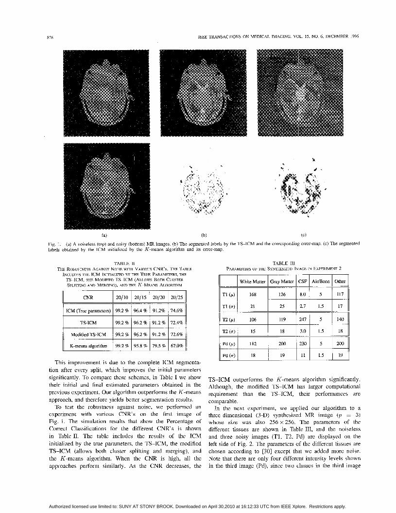
In Fig. 1, the left two images are a noiseless (top) and noisy (bottom) MR images, and the middle two images are the segmented image by the TS-ICM and the corresponding error- map. The two images on the right are the segmented image obtained by the ICM initialized by the K-means algorithm and its error-map. When we simulated the K-means algorithm, we updated the parameters {p l , CT~} after each iteration [46]. The results clearly show improved performance of our procedure over the K-means procedure.


876

CNR

ICM (True parameters)

TS-ICM

Modified TS-ICM

K-means algorithm

IEEE TRANSACTIONS ON MEDICAL IMAGING, VOL. 15, NO. 6, DECEMBER 1996

20110 20115

99.2 % 96.4 %

99.2 % 96.2 %

99.2 % 96.2 %

99.2 % 95.8 %

Fig. 1. labels obtained by the ICM initialized by the K-means algorithm and its error-map.

(a) A noiseless (top) and noisy (bottom) MR images. (b) The segmented labels by the TS-ICM and the corresponding error-map. (c) The segmented

TABLE I1 THE ROBUSTNESS AGAINST NOISE WITH VARIOUS CNR'S. THE TABLE

INCLUDES THE ICM INITIALIZED BY THE TRUE PARAMETERS, THE TS-ICM, THE MODIFIED TS-ICM (ALLOWS BOTH CLUSTER SPLITKNG AND MERGING), AND THE &MEANS ALGORITHM

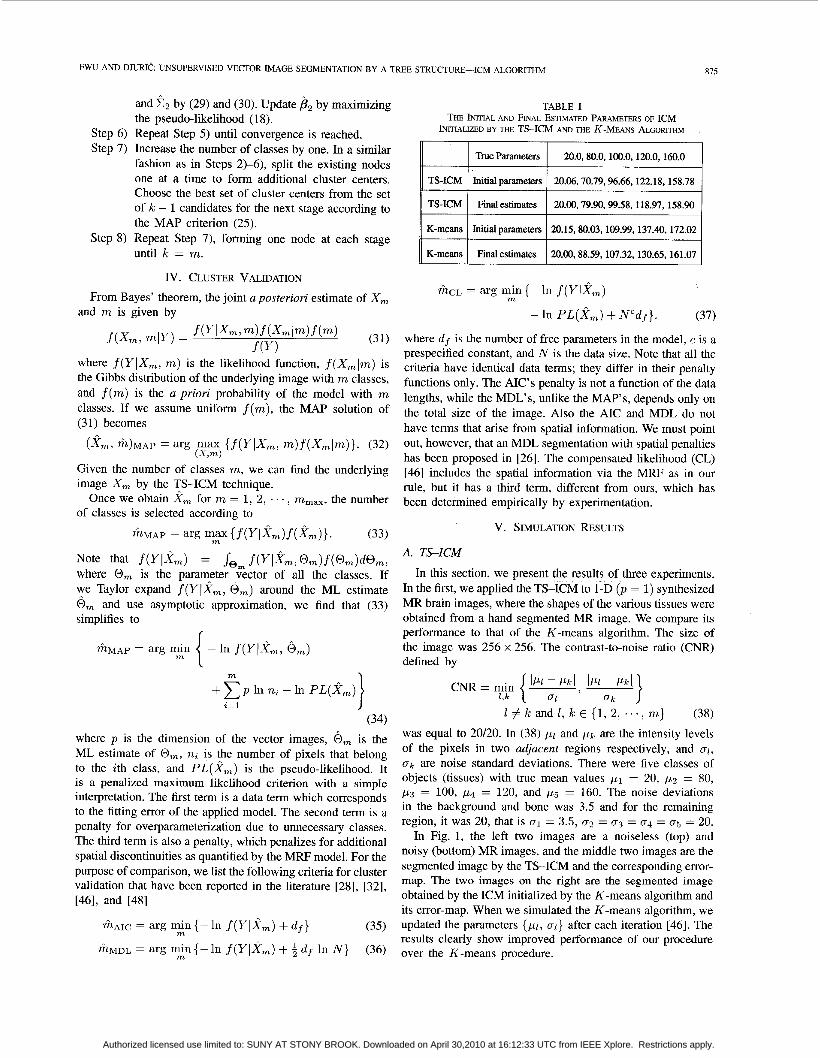
This improvement is due to the complete ICM segmentation after every split, which improves the initial parameters significantly. To compare these schemes, in Table I we show their initial and final estimated parameters obtained in the previous experiment. Our algorithm outperforms the K-means approach, and therefore yields better segmentation results.

To test the robustness against noise, we performed an experiment with various CNR's on the first image of Fig. 1. The simulation results that show the Percentage of Correct Classifications for the different CNR's is shown in Table 11. The table includes the results of the ICM initialized by the true parameters, the TS-ICM, the modified TS-ICM (allows both cluster splitting and merging), and the K-means algorithm. When the CNR is high, all the approaches perform similarly. As the CNR decreases, the

TABLE I11 PARAMETERS OF THE SYNTHESIZED IMAGE IN EXPERIMENT 2

T1 ( p ) 168

T1 (c) 21 25

T 2 ( p ) 106 119 I I I U

TS-ICM outperforms the K-means algorithm significantly. Although, the modified TS-ICM has larger computational requirement than the TS-ICM, their performances are comparable.

In the next experiment, we applied our algorithm to a three-dimensional (3-D) synthesized MR image (I, = 3) whose size was also 256 x 256. The parameters of the different tissues are shown in Table 111, and the noiseless and three noisy images (Tl, T2, Pd) are displayed on the left side of Fig. 2. The parameters of the different tissues are chosen according to [30] except that we added more noise. Note that there are only four different intensity levels shown in the third image (Pd), since two classes in the third image


FWU AND DJURIC: UNSUPERVISED VECTOR IMAGE SEGMENTATION BY A TREE STRUCTURE-ICM ALGORITHM 817

(a) (b)

Fig. 2. (a) The class labels of the underlying image, and the three bands of the noisy synthesized MR images. (b) The top two images display the segmented labels and the error-map of the TS-ICM. The bottom two images are the segmented labels and the error-map of the ICM initialized by the A-means algorithm.

have the same intensity level. In addition, the white matter and gray matter are two adjacent regions with small CNR, which makes them difficult for discrimination.

In Fig. 2, the top two images on the right side display the segmentation result and the error-map of the TS-ICM. The bottom two images on the right display the segmentation result and the error-map of the ICM initialized by the K-

means algorithm. Table IV shows the numbers of misclassified pixels in various regions obtained by the ICM initialized by the TS and the K-means algorithm, respectively. Clearly, the TS algorithm had better performance, and it is more so as we keep increasing the noise. In our experiments the algorithm created a few 1-pixel regions, which can be prevented by additional penalization.


878 EEE TRANSACTIONS ON MEDICAL IMAGING, VOL. 15, NO. 6, DECEMBER 1996

TS-ICM

ICM initialized by the K-means algorithm

TABLE IV THE NUMBER OF MISCLASSIFIED PIXELS IN VARIOUS REGIONS FOR ICM INmIALIZED BY THE TS-ICM AND THE K-MEANS ALGORITHM

WhiteMatter GrayMatter CSF Air/Bone Other

181 311 3 0 11

248 507 3 0 8

ImageSidCNR

TABLE V COMPARISON OF THE MAP, AIC, AND MDL RULES FOR

QUSTER VALIDATION. THE TRUE NUMBER OF CLASSED IS FIVE

rule\segm. 2 3 4 5 6 7

In the last experiment, we applied our algorithm to a real 3-D MR image (Tl, T2, and Pd) acquired by a 1.5-Tesla GE scanner, whose size was also 256 x 256. In Fig. 3, the images on the left side from top to bottom, are the T1, T2, and Pd images. The T1 image is acquired with TR = 1000 ms and TE = 20 ms, the T2 image with TR = 2000 and TE = 75 ms, and the Pd image with TR = 3000 and TE = 20 ms. The images on the right hand side from top to bottom, are the segmentation results for m = 4, 5 , and 6, respectively.

B. Cluster Validation

To verify the cluster validation performance of the proposed MAP criterion, we applied it to the synthesized MR brain images as shown in Fig. 2. Table V displays the simulation results from 50 independent trials of the MAP, AIC, and MDL rules. As can be seen, the AIC and MDL showed strong tendencies to overestimate the number of classes. In particular, the AIC exhibited very poor performance and can be considered unreliable. By contrast, our criterion yielded excellent results.

20/2 20/4 20/6 2W8 20/10 20/12

VI. DISCUSSION

A. Sensitivity Evaluation

Cluster splitting can only perform well if the clusters contain large enough number of pixels, and there seems no obvious way to circumvent this problem. In order to examine this issue, we generated a small region (10 x 10 pixels) embedded in a larger region with different CNR’s. The experiment was performed with various vector images who sizes were 32 x 32, 64 x 64, and 128 x 128 pixels. The results are listed in Table VI, where the entries represent the misclassified pixels (average value out of 50 trials) and “F” denotes more than 35 misclassified pixels or failure of discrimination.

As the image size gets larger, the required CNR for suc- cessful separation of the small object from the background increases. This shows that a subcluster can only be separated from the other cluster if its size is not too small compared to the other one. Of course, this also depends on the CNR. For

TABLE VI SENSITIVITY ANALYSIS OF THE TS-ICM ALGORITHM

example, at CNR = 2/1, the small object can be separated from the larger one, if their size ratio is larger than 1/10.

B. Computational EfJiciency It is known that the ICM is an efficient algorithm, when

the class parameters are known. If the initial conditions are unknown, the TS algorithm provides an efficient way for obtaining them. The TS algorithm when applied to a 3-D (Tl, T2, and Pd) 256 x 256 brain image with five classes, takes about 12 min on a Pentium 90 machine with 16 MB RAM and 32-MB swap memory. Although Dubes et al. [ 111 show that the ICM can converge in five or six raster scans of an image, we performed ten raster scans for the segmentations in our simulations.

The computational requirements mainly depend on the image size and the number of classes contained in the image. It does not vary dramatically when it is applied to different types of images. When the image has m different classes, the total computation requirement is z = m2 - m - 1 segmentations. For a medium size image (e.g., 256 x 256) with a medium number of classes (e.g., lo), the computational requirements are modest. When the image size and the number of classes are large, as can occur, for example, in some satellite image applications, the direct application of the TS algorithm may become computationally infeasible. Since a significant portion of the computation is used for initialization, to reduce the computational requirements, coarse segmentation can be applied to feature vectors extracted from 6 x b windows. Once the initial parameters are obtained, the segmentation can proceed as before. In some practical applications, this may decrease the computation by a factor of about l / b 2 . In certain cases, however, a technique based on this approach may miss some extremely narrow regions. Another way to reduce the computational requirement in applications with larger number of classes is to start the TS-ICM from certain number of classes rather than always starting from one class. In addition, parallel computation can be straightforwardly applied which will further reduce the computation time.

m-1 .


m u AND DJURIC: UNSUPERVISED VECTOR IMAGE SEGMENTATION BY A TREE STRUCTURE--ICM ALGORITHM

Fig. 3. (a)

(a)

Three bands of the noisy real MR images (T1

(b)

T2, and Pd weighted). (b) From top to bottom, the segmented m = 4, 5, and 6, respectively.

VII. CONCLUSIONS

We have presented a novel algorithm for simultaneous parameter estimation and vector image segmentation. The algorithm is implemented sequentially in stages, where at each stage a specific number of classes is assumed. It increases the number of classes by one at each stage by using a tree

structure technique that provides initial parameter which are then improved by the ICM procedure. mation results of every stage are used as initial

879

labels for

estimates The esti- estimates

for the next stage. As the number of stages increases, the number of classes also increases. We have also proposed a MAP criterion for cluster validation. This criterion has the



_- form of a penalized likelihood function that is composed [22] A. K. Jain and R. C. Dubes, Algorithms for Clustering Data. Engle- of two terms, a data term and a penalty term. The data term represents the fitness of the segmented image to the original image, and the penalty term penalizes for the spatial discontinuity and the overparameterization. The performance of the algorithm and the MAP criterion were examined by computer simulations on synthesized images, and they show excellent results. Segmentation results on real brain images are also included.

ACKNOWLEDGMENT The authors are grateful to Prof. N. Phamdo for many

fruitful suggestions and discussions, as well as to the reviewers for their constructive comments and suggestions, which have greatly improved this manuscript.

REFERENCES

[l] H. Akaike, “A new look at the statistical model identification,” IEEE Trans. Automat. Contr., vol. AC-19, pp. 716723, 1974.

[2] G. H. Ball and D. J. Hall, “A clustering technique for summarizing multivariate data,” Behavioral Sei., vol. 12, pp. 153-155, 1967.

[3] J. D. Banfield and A. E. Raftery, “Model-based Gaussian and non- Gaussian clustering,” Biometrics, pp. 803-821, 1993.

[4] J. Besag, “On the statistical analysis of dirty pictures,” J. Roy. Stat. Soc., ser. B, vol. 48, no. 3, pp. 259-302, 1986.

[5] -, “Spatial interaction and statistical analysis of lattice systems,” J. Roy. Stat. Soc., ser. B, vol. 36, pp. 192-236, 1974.

[6] C. Bouman and B. Liu, “Multiple resolution segmentation of texture images,” IEEE Trans. Pattem Anal. Machine Intell., vol. 13, pp. 99-1 13, 1991.

171 C. Bouman and M. Shapiro, “A multiscale random field model for Bayesian image segmentation,” IEEE Trans. Imane Processing, vol. 3, pp: 162-177,-1994.

I81 C. C. Chu and J. K. Agganval, “The integration of image segmentation _ _ ~~

maps using region and edge information,” IEEE Trans. Puttem Anal. Machine Intell., vol. 15, pp. 1241-1252, 1993.

191 A. P. Dempster, N. M. Laird, and D. B. Rubin, ‘‘ Maximum likelihood from incomplete data via the EM algorithm,” J. Roy. Stat. Soc., ser. B, vol. 39, no. 1, pp. 1-38, 1977.

[lo] P. M. DjuriC, “Model selection based on asymptotic Bayes theory,” in Proc. 7th SP Workshop on Statistical Signal & Array Processing, 1994, pp. 7-10.

[ l l ] R. C. Dubes, A. K. Jain, S. G. Nadabar, and C. C. Chen, “MRF model-based algorithms for image segmentation,” in IEEE Conf Pattern

- I

Recog.., 1990, pp . 808-814. r121 R. 0. Duda and P. E. Hart, Pattem Classification and Scene Analvsis. . .

New York: Wiley, 1973, pp. 332-335. [13] B. S. Everitt, Finite Mixture Distributions. Chapman-Hall, 1981. [14] D. Geiger and F. Girosi, “Parallel and deterministic algorithms from

MRF’s: Surface reconstruction,” IEEE Trans. Pattem Anal. Machine Intell., vol. 13, pp. 401412, 1991.

[15] S. Geman and D. Geman, “Stochastic relaxation, Gibbs distributions, and the Bayesian restoration of images,” IEEE Trans. Pattern Anal. Machine Intell., vol. PAMI-6, pp. 721-741, 1984.

[ 161 A. Gersho and R. M. Gray, Vector Quantization and Signal Compression. Boston: Kluwer, 1991, pp. 309423.

[17] R. M. Gray, “Vector quantization,” IEEE Acout. Speech, Signal Process- ing Mag., vol. ASSP-1, pp. 4-29, 1984.

[l8] Y. S. Han and W. E. Snyder, “Discontinuity-preserving vector smooth- ing on multivariate MR images via vector mean field annealing,” Proc. SPIE Math. Methods Med. Imag., pp. 69-80, 1992.

[19] J. A Hartigan, Clustering Algorithms. New York: Wiley , 1975, pp. 84-125.

[20] F. Heitz, P. Perez, and P. Boutbemy, “Multiscale minimization of global energy functions in some visual recovery problems,” CVGIP: Image Understanding, vol. 59, pp. 125-134, 1994.

[21] C. L. Huang, T. Y. Cheng, and C. C. Chen, “Color images’ segmentation using scale space filter and Markov random field,” Pattem Recog., vol. 25, pp. 1217-1229, 1992.

wood Cliffs, NJ: Prentice Hall, 1988. [23] F. C. Jeng and J. W. Wood, “Compound Gauss-Markov random fields

for image estimation,” IEEE Trans. Signal Processing, vol. 39, pp. 683-697, 1991.

[24] R. E. Kass and A. E. Raftery, “Bayes factors,” J. Amer. Stat. Assoc.,

[25] Z. Kato, J. Zerubia, and M. Berthod, “Unsupervised adaptive image segmentation,’’ in Proc. ICASSP, 1995, pp. 2399-2402.

[26] I. B. Kerfoot and Y. Bresler, “Design and theoretical analysis of a vector field segmentation algorithm,” in Proc. ICASSP, 1993, vol. 5, pp. 5-8.

1271 R. Kindermann and J. L. Snell, Markov Random Fields and Their Applications. Providence, RI: American Mathematical Society, 1980, vol. 1.

[28] D. A. Langan, J. W. Modestino, and J. Zhang, “Cluster validation for unsupervised stochastic model-based image segmentation,” in Proc.

[29] S. Lakshmanan and H. Derin, “Simultaneous parameter estimation and segmentation of Gibbs random fields using simulated annealing,” IEEE Trans. Pattem Anal. Machine Intell., vol. 11, pp. 799-813, 1989.

[30] R. Leahy, T. Hebert, and R. Lee, “Applications of Markov random fields in medical imaging,” in Proc. 11th Int. Conf Inform. Processing Med.

vol. 90, pp. 737-795, 1995.

ICIP, 1994, vol. 2 , pp. 197-201.

- _ . .

Imag., 1989, pp. 1-14. 1311 Y. G. Leclerc, “Constructing simple stable descriptions for image ~~

partitioning,” Int. J. Comput. Vision, vol. 3, pp. 73-102, 1989. [32] Z. Liang, R. J. Jaszczak, and R. E. Coleman, “Parameter estimation

of finite mixtures using EM algorithm and information criteria with application to medical image processing,” IEEE Trans. Nucl. Sci., vol. 39, pp. 1126-1133, 1992.

[33] J. Marroquin, S. Mitter, and T. Poggio, “Probabilistic solution of ill- posed problems in comuutational vision,” J. Amer. Star. Assoc., vol. 82, pp. 76-89, 1987.

1341 P. Masson and W. Pieczynski, “SEM algorithm and unsupervised ~~

statistical segmentation of satellite images,” G E E Trans. Geosci.-Remote Sensing, vol. 31, pp. 618-633, 1993.

[35] K. L. Oehler and R. M. Gray, “Combining image compression and classification using vector quantization,” IEEE Trans. Pattem Anal. Machine Intell., vol. 17, pp. 461-473, 1995.

[36] D. K. Panjwani and G. Healey, “Unsupervised segmentation of textured color images using Markov random field models,” in IEEE Con$ Comput. Vision and Pattem Recog., 1993, pp. 776-717.

[37] T. N. Pappas, “An adaptive clustering algorithm for image segmentation,” IEEE Trans. Signal Processing, vol. 40, pp. 901-914, 1992.

[38] N. Phamdo, N. Farvardin, and T. Moriya, “A unified approach to tree- structure and multistage vector quantization for noisy channels,” IEEE Trans. Inform. Theoly, vol. 39, pp. 835-850, 1993.

[39] I. Pitas and A. N. Venetsanopoulos, “Order statistics in digital image processing,” Proc. IEEE, pp. 1893-1921, 1992.

[40] I. Pitas and P. Tsakalides, “Multivariate ordering in color image filter- ing,” IEEE Trans. Circ. Syst. Video Tech., vol. 1, pp. 241-259, 1991.

[41] J. G. Postaire and C. P. A. Vasseur, “An approximate solution to normal mixture identification with application to unsupervised pattern classification,” IEEE Trans. Pattem Anal. Machine Intell., vol. PAMI-3, pp. 163-179, 1981.

r421 E. Rignot and R. Chellappa, “Segmentation of polarimetric synthetic . .

apert& radar data,” I E E i k zns . Image Processing, vol. 1, pp. 281-300, 1992.

[43] E. A. Riskin and R. M. Gray, “A greedy tree growing algorithm for the design of variable rate vector quantizers,” IEEE Trans. Signal Processing, vol. 39, pp. 2500-2507, 1991.

[44] J. Rissanen, “Modeling by shortest data description,” Automatica, vol. 14, pp. 465478, 1978.

[45] J. T. Tou and R. C. Gonzalez, Pattem Recognition Principles. Reading, MA: Addison-Wesley, 1974.

[46] C. Won and H. Derin, “Unsupervised segmentation of noisy and textured images using Markov random fields,” CVGIP: Graphical Models and Image Processing, vol. 54, pp. 308-328, 1992.

[47] J. C. Yen, F. J. Chang, and S Chang, “A new criterion for automatic multilevel thresholding,” IEEE Trans. Image Processing, vol. 4, pp. 370-378, 1995.

[48] J. Zhang and J. W. Modestino, “A model-fitting approach to cluster validation with application to stochastic model-base image segmentation,’’ IEEE Trans. Pattern Anal. Machine Intell., vol. 12, pp. 1009-1017, 1990.

[49] J. Zhang, “The mean fields theory in EM procedures for Markov random fields,” IEEE Trans. Signal Processing, vol. 40, pp. 2570-2583, 1992.


Unsupervised Vector Image Segmentation by a Tree Structure-ICM

Documents

Transcript of Unsupervised Vector Image Segmentation by a Tree Structure-ICM