Unsupervised Segmentation of Head Tissues from...
81
THESIS FOR THE DEGREE OF DOCTOR OF PHILOSOPHY Unsupervised Segmentation of Head Tissues from Multi-Modal Magnetic Resonance Images: With Application to EEG Source Localization and Stroke Detection QAISER MAHMOOD Department of Signals and Systems CHALMERS UNIVERSITY OF TECHNOLOGY Gothenburg, Sweden 2016
Transcript of Unsupervised Segmentation of Head Tissues from...

THESIS FOR THE DEGREE OF DOCTOR OF PHILOSOPHY
Unsupervised Segmentation of Head Tissues fromMulti-Modal Magnetic Resonance Images: With Application
to EEG Source Localization and Stroke Detection
QAISER MAHMOOD
Department of Signals and SystemsCHALMERS UNIVERSITY OF TECHNOLOGY
Gothenburg, Sweden 2016

Unsupervised Segmentation of Head Tissues from Multi-Modal Magnetic ResonanceImages: With Application to EEG Source Localization and Stroke DetectionQAISER MAHMOOD
ISBN 978-91-7597-339-5
This thesis has been prepared using LATEX.Copyright c© QAISER MAHMOOD, 2016.All rights reserved.
Doktorsavhandlingar vid Chalmers Tekniska HogskolaNy serie nr 4020ISSN 0346-718X
Department of Signals and SystemsImaging and Image Analysis GroupChalmers University of TechnologySE-412 96 Gothenburg, SwedenPhone: +46 (0)31 772 1583Fax: +46 (0)31 772 1725E-mail: [email protected]
Printed by Chalmers ReproserviceGothenburg, Sweden, 2016

TO MY BELOVED PARENTS AND ZOHRA


Abstract
The automated segmentation or labeling of individual tissues in magnetic resonance (MR) im-ages of the human head is an essential first step in several biomedical applications. The resultingsegmentation yields a patient-specific labeling of individual tissues that can be used to quantita-tively characterize these tissues (e.g. in the study of Alzheimers disease and multiple sclerosis)or to assign individual dielectric properties for patient-specific electromagnetic simulations (e.g.in applications such as electroencephalography source localization in epilepsy patients and mi-crowave imaging for stroke detection). Automated and accurate segmentation of MR images isa challenging task because of the complexity and variability of the underlying anatomy and thenoise and the bias field (spatial intensity inhomogeneities). Consequently, manual segmentation,including both interactive segmentation and manual correction, is largely used in clinical research.However, it is time consuming, subjective, tedious, and labor-intensive. This thesis presents newsegmentation methods for both the brain and whole-head that are both automatic and accurate. Italso presents empirical evaluations of these methods both directly in terms of segmentation accu-racy and indirectly in terms of efficacy in electroencephalography (EEG) source localization andstroke detection. The evaluations were performed using both synthetic and real MRI data. Thisthesis makes four distinct contributions. The first is a novel unsupervised segmentation frame-work for segmenting MR images of the brain into three tissue types: white matter, gray matterand cerebrospinal fluid. It is a combination of Bayesian-based adaptive mean shift, incorporat-ing an a priori tissue label probability maps, and the fuzzy c-means algorithm. The experimentalresults —based on both synthetic T1-weighted MR images for different noise levels and spatialintensity inhomogeneity levels, and real T1-weighted MR images —demonstrate its robustnessand that it has a higher degree of segmentation accuracy than existing methods. The second is anovel automated unsupervised whole-head segmentation method for the purpose of constructinga patient-specific dielectric or biomechanical head model. The method is based on a hierarchicalsegmentation approach incorporating Bayesian-based adaptive mean shift. The experimental re-sults demonstrate the efficacy of the proposed method, its robustness to noise and the bias field,and that it has a higher degree of segmentation accuracy than existing methods. The third is anevaluation of the proposed whole-head segmentation method in the context of EEG source lo-calization. The experimental results show that the proposed method yields improved localizationaccuracy over the commonly used method for constructing a realistic head conductivity model forEEG source localization. The fourth is an evaluation of several existing unsupervised segmen-tation methods including the proposed whole-head segmentation method in the context of strokedetection using a microwave imaging system. The experimental results show that the proposedmethod has higher image reconstruction accuracy for intracerebral hemorrhage compared to theexisting methods. The results also suggest that accurate automated segmentation can be used asa surrogate for manual segmentation to obtain accurate image reconstruction of an intracerebralhemorrhage and can assist in real time stroke detection.Keywords: Image segmentation, magnetic resonance, brain, EEG source localization, stroke, re-construction

ii

Preface
This thesis is in partial fulfillment of the requirements for the degree of Doctor of Philosophy atChalmers University of Technology, Gothenburg, Sweden.
The work herein was jointly undertaken in the Imaging and Image Analysis Group within theDepartment of Signals and Systems at Chalmers University of Technology, and MedTech Westlocated at Sahlgrenska University Hospital (both in Gothenburg, Sweden) between September2010 and December 2015. It was performed under the joint supervision of Professor MikaelPersson, Dr. Artur Chodorowski and Associate Prof. Andrew Mehnert. Prof. Persson also acts asexaminer of the thesis.
This work has been supported in parts by the Chalmers University of Technology and theHigher Education Commission (HEC) of Pakistan. Some of the MRI data in this thesis was ac-quired by the Department of Clinical Neurophysiology, Sahlgrenska University Hospital, Gothen-burg, Sweden.
iii

iv

List of Publications
This thesis is based on the work contained in the following papers:
Paper AQaiser Mahmood, Artur Chodorowski, Andrew Mehnert, Mikael Persson, “A Novel BayesianApproach to Adaptive Mean Shift Segmentation of Brain Images”, Proceedings of IEEE Interna-tional Conference on Computer Based Medical Systems (CBMS), pp. 1-6, Rome, Italy, 20th-22ndJune, 2012.
Paper BQaiser Mahmood, Artur Chodorowski, Mikael Persson, “Automated MRI Brain Tissue Segmen-tation based on Mean Shift and Fuzzy C-Means using a Priori Tissue Probability Maps”, Innova-tion and Research in BioMedical Engineering (IRBM), pp.185-196, 2015.
Paper CYazdan Shirvany, Antonio R. Porras, Koushyar Kowkabzadeh, Qaiser Mahmood, Hoi-Shun Lui,Mikael Persson, “Investigation of Brain Tissue Segmentation Error and its Effect on EEG SourceLocalization”, Proceedings of International Conference of the IEEE Engineering in Medicine andBiology Society (EMBC), pp. 1522-1525, San Diego, USA, 22nd Aug.-1st Sep., 2012.
Paper DYazdan Shirvany, Qaiser Mahmood, Fredrik Edelvik, Stefan Jakobsson, Anders Hedstrom, MikaelPersson, “Particle Swarm Optimization Applied to EEG Source Localization of SomatosensoryEvoked Potentials”, IEEE Transactions on Neural Systems and Rehabilitation Engineering, pp.11- 20, 2013.
Paper EQaiser Mahmood, Artur Chodorowski, Andrew Mehnert, Johanna Gellermann, Mikael Persson,“Unsupervised Segmentation of Head Tissues from Multi-modal MR Images for EEG Source Lo-calization”, Journal of Digital Imaging (JDI), pp. 1-16, 2014, DOI:10.1007/s10278-014-9752-6.
Paper FQaiser Mahmood, Shaochuan Li, Andreas Fhager, Stefan Candefjord, Artur Chodorowski, An-drew Mehnert, Mikael Persson, “A Comparative Study of Automated Segmentation Methods forUse in a Microwave Tomography System for Imaging Intracerebral Hemorrhage in Stroke Pa-tients”, Journal of Electromagnetic Analysis and Applications (JEMAA), Online, May 2015.
v

Other related publications by the author not included in this thesis:
Peer reviewed
1. Mikael Persson, Tomas McKelvey, Andreas Fhager, Hoi-Shun Lu, Yazdan Shirvany, ArturChodorowski, Qaiser Mahmood, Fredrik Edelvik, Magnus Thordstein, Anders Hedstrom,Mikael Elam, “Advances in Neuro Diagnostic Based on Microwave Technology, Transcra-nial Magnetic Stimulation and EEG source localization”, Proceedings of Asia-Pacific Mi-crowave Conference, Melbourne, Australia, 5th-8th Dec., 2011.
2. Yazdan Shirvany, Fredrik Edelvik, Stefan Jakobsson, Anders Hedstrom, Qaiser Mahmood,Artur Chodorowski and Mikael Persson, “Non-invasive EEG source localization with Parti-cle Swarm Optimization: Clinical Test”, Proceedings International Conference of the IEEEEngineering in Medicine and Biology Society (EMBC), pp. 6232-6235, San Diego, 22ndAug.-1st Sep., 2012.
3. Qaiser Mahmood, Yazdan Shirvany, Andrew Mehnert, Artur Chodorowski, Johanna Geller-mann, Fredrik Edelvik, Anders Hedstrom, Mikael Persson, “On the Fully Automatic Con-struction of a Realistic Head Model for EEG Source Localization”, Proceedings of Interna-tional Conference of the IEEE Engineering in Medicine and Biology Society (EMBC), pp.3331-3334, Osaka, Japan, 3rd-7th, July 2013.
4. Qaiser Mahmood, Artur Chodorowski, Babak Ehteshami Bejnordi, Mikael Persson, “AFully Automatic Unsupervised Segmentation Framework for the Brain Tissues in MR Im-ages”, SPIE Medical Imaging, Biomedical Applications in Molecular, Structural, and Func-tional Imaging, Volume 9038, 2014.
Non peer reviewed
1. Qaiser Mahmood, Artur Chodorowski, Mikael Persson, “Adaptive Segmentation of BrainTissues from MR Images”, Proceedings of Medicinteknikdagarna, p.86, Linkoping, Swe-den, 11th-12th Oct., 2011.
2. Qaiser Mahmood, Artur Chodorowski, Andrew Mehnert, Johanna Gellermann, MikaelPersson, “Bayesian Based Adaptive Mean Shift Algorithm for Automatic Multi-TissueSegmentation of the Human Head”, Proceedings of Medicinteknikdagarna, p.158, Lund,Sweden, 2nd-3rd Oct., 2012.
3. Qaiser Mahmood, Yazdan Shirvany, Andrew Mehnert, Artur Chodorowski, Johanna Geller-mann, Fredrik Edelvik, Anders Hedstrom, Mikael Persson, “On the Fully Automatic Con-struction of a Realistic Head Model for EEG Source Localization”, Proceedings of SwedishSymposium on Image Analysis (SSBA), Goteborg, Sweden, 14th-15th March, 2013.
4. Qaiser Mahmood, Artur Chodorowski, Mikael Persson, “Multi-modal Tumor Brain Seg-mentation”, Rontgennvecka, Uppsala, Sweden, 2nd-6th Sept, 2013.
5. Qaiser Mahmood, Artur Chodorowski, Mikael Persson, “A Fully Automatic UnsupervisedSegmentation Framework for the Brain Tissues in MR Images”, Proceedings of Medicin-teknikdagarna, Goteborg, Sweden, 14th-16th Oct., 2014.
vi

Acknowledgments
I would like to express my gratitude to all those who gave me the possibility to complete thisthesis.
First of all I would like to thank my supervisor Prof. Mikael Persson for his support through-out the research work and giving the freedom to pursue the research directions I am interestedin. I would like to express my deep gratitude to Dr. Artur Chodorowski and Associate Prof.Andrew Mehnert, my co-supervisors, for their patient guidance, enthusiastic encouragement anduseful critiques of this research work. I would like to express my very great appreciation to Dr.Johanna Gellermann for generating real patient ground truth images and also for sharing with meher wide MRI expertise in numerous interesting discussions. I would like also to thank AssociateProf. Fredrik Edelvik from Fraunhofer-Chalmers Research Center and Dr. Yazdan Shirvany forgiving me the opportunity to apply this work to the EEG source localization problem in epilepsy.I am very grateful to Associate Prof. Andreas Fhager from Department of Signals and Systems atChalmers University of Technology for his valuable feedback and enthusiasm with pushing thiswork towards stroke detection. I would like to acknowledge the Department of Clinical Neuro-physiology at Sahlgrenska University Hospital, Gothenburg for providing real MRI patient data. Iextend a special thanks to Dr. Irene Perini for her advice and input on the anatomy of the humanhead.
I would like to thank to Dr. Markus Johansson, Dr. Stefan Candefjord, Prof. Rolf Heckemann,Associate Prof. Justin Schneiderman and Henrik Mindedal from MedTech West at SahlgrenskaUniversity Hospital and all colleagues, in particular Ann-Christine Lindbom and Natasha Adlerfrom Department of Signals and Systems at Chalmers University of Technology for their kind-ness, cooperation, and support. I wish to thank all my friends especially Shahid Nawaz, Qaisar,Mohammad Alipoor, Mats Lindstrom, Georgi, Martina, Rhys Lewis, Cristina, Ramin and Babakfor their support and creating enjoyable moments in my life. I am grateful to the Higher EducationCommission (HEC) of Pakistan and Chalmers University of Technology, Sweden for providingme the scholarship to conduct this research.
Most importantly, none of this would have been possible without the love and patience of myfamily. I would like to express my heart felt gratitude to my loving parents, brothers and sistersand their families for their support and encouragement.
Qaiser Mahmood, Gothenburg, 2016
vii

viii

Abbreviations and Acronyms
AMS Adaptive Mean ShiftBAMS Bayesian-Based Adaptive Mean ShiftBET Brain Extraction ToolBT Brain TissueCSF Cerebrospinal FluidCT Computed TomographyDI Dice IndexEEG ElectroencephalographyEM Expectation MaximizationFAST FMRIB’s Automated Segmentation ToolFCM Fuzzy C-MeansFID Free Induction DecayFDTD Finite Difference Time DomainFMRIB Functional MRI of the BrainFSL FMRIB Software LibraryGE Gradient EchoGM Gray MatterGMM Gaussian Mixture ModelGT Ground TruthHMRF Hidden Markov Random FieldHSA Hierarchical Segmentation ApproachIBSR Internet Brain Segmentation RepositoryICM Iterated Conditional ModesLE Localization ErrorMRF Markov Random FieldMRI Magnetic Resonance ImagingMTSA Multi-tissue Segmentation AlgorithmMS Mean ShiftNBT Non-Brain TissueOE Orientation ErrorPD Proton DensityPVC Partial Volume ClassifierRE Relative ErrorRF Radio FrequencySPM Statistical Parametric Mapping
ix

SE Spin EchoT1 Longitudinal Relaxation TimeT2 Transverse Relaxation TimeTE Echo TimeTR Repetition TimeWM White MatterWHSA Whole Head Segmentation Algorithm
x
Contents
Abstract i
Preface iii
List of Publications v
Acknowledgments vii
Abbreviations and Acronyms ix
Contents xi
Part I: Introductory Chapters 1
1 Introduction 31.1 Background and problem definition . . . . . . . . . . . . . . . . . . . . 31.2 Aim and objectives . . . . . . . . . . . . . . . . . . . . . . . . . . . . . 41.3 Scope of the thesis . . . . . . . . . . . . . . . . . . . . . . . . . . . . . 51.4 Overview of the thesis . . . . . . . . . . . . . . . . . . . . . . . . . . . 5
2 Theoretical Background 72.1 Anatomy of the human head . . . . . . . . . . . . . . . . . . . . . . . . 7
2.1.1 Brain . . . . . . . . . . . . . . . . . . . . . . . . . . . . . . . . 82.1.2 Non-brain . . . . . . . . . . . . . . . . . . . . . . . . . . . . . . 9
2.2 Magnetic Resonance Imaging (MRI) . . . . . . . . . . . . . . . . . . . . 92.2.1 Contrast Mechanisms in MRI . . . . . . . . . . . . . . . . . . . 122.2.2 Basic pulse sequences for MRI . . . . . . . . . . . . . . . . . . . 142.2.3 Artifacts in MRI . . . . . . . . . . . . . . . . . . . . . . . . . . 14
2.3 Overview of the basic segmentation techniques underlying existing ap-proaches to brain and whole-head segmentation . . . . . . . . . . . . . . 15
3 MRI Brain Tissue Segmentation 213.1 MRI brain tissue segmentation methods: A review . . . . . . . . . . . . 213.2 Proposed unsupervised segmentation framework . . . . . . . . . . . . . . 223.3 Empirical evaluation of the proposed framework . . . . . . . . . . . . . . 24
xi
4 MRI Whole-Head Tissue Segmentation 294.1 Automated head tissue segmentation: Motivation . . . . . . . . . . . . . 294.2 Proposed whole-head segmentation method . . . . . . . . . . . . . . . . 294.3 Empirical evaluation of the proposed method . . . . . . . . . . . . . . . 30
5 MRI Whole-Head Tissue Segmentation: Application to EEG Source Local-ization 355.1 Automated head tissue segmentation for EEG source localization: Moti-
vation . . . . . . . . . . . . . . . . . . . . . . . . . . . . . . . . . . . . 355.2 The EEG Source Localization Problem . . . . . . . . . . . . . . . . . . 365.3 Evaluation of the proposed whole-head tissue segmentation method: EEG
source localization accuracy . . . . . . . . . . . . . . . . . . . . . . . . 36
6 MRI Whole-Head Tissue Segmentation: Application to Hemorrhagic StrokeDetection 396.1 Application: Detecting Hemorrhagic Stroke with Microwave-Imaging . . 39
6.1.1 Image reconstruction for intracerebral hemorrhage . . . . . . . . 406.2 Evaluation of segmentation methods: Intracerebral hemorrhage detection 41
6.2.1 Automated segmentation methods . . . . . . . . . . . . . . . . . 42
7 Summary of the papers 477.1 Brain Segmentation . . . . . . . . . . . . . . . . . . . . . . . . . . . . . 47
7.1.1 Paper A: A Novel Bayesian Approach to Adaptive Mean ShiftSegmentation of Brain Images . . . . . . . . . . . . . . . . . . . 47
7.1.2 Paper B: Automated MRI Brain Tissue Segmentation based onMean Shift and Fuzzy C-Means using a Priori Tissue ProbabilityMaps . . . . . . . . . . . . . . . . . . . . . . . . . . . . . . . . 48
7.2 MRI Whole-Head Segmentation: EEG Source Localization . . . . . . . . 487.2.1 Paper C: Investigation of Brain Tissue Segmentation Error and Its
Effect on EEG Source Localization . . . . . . . . . . . . . . . . 487.2.2 Paper D: Particle Swarm Optimization Applied to EEG Source
Localization of Somatosensory Evoked Potentials . . . . . . . . . 497.2.3 Paper E: Unsupervised Segmentation of Head Tissues from Multi-
modal MR Images for EEG Source Localization . . . . . . . . . 497.3 MRI Whole-Head Segmentation: Intracerebral Hemorrhage Detection in
Stroke Patients . . . . . . . . . . . . . . . . . . . . . . . . . . . . . . . 507.3.1 Paper F: A Comparative Study of Automated Segmentation Meth-
ods for Use in a Microwave Tomography System for Imaging In-tracerebral Hemorrhage in Stroke Patients . . . . . . . . . . . . . 50
8 Conclusions and Outlook 518.1 Conclusions . . . . . . . . . . . . . . . . . . . . . . . . . . . . . . . . . 518.2 Future work . . . . . . . . . . . . . . . . . . . . . . . . . . . . . . . . . 52
xii

References 55
Part II: Included Papers A-F 65
xiii


Part IIntroductory Chapters
1


CHAPTER 1
Introduction
1.1 Background and problem definition
Medical imaging [1–3] is the visualization of body parts, tissues, or organs, for use inclinical diagnosis, treatment and disease monitoring. It plays an important role in theglobal healthcare system as it contributes to improved patient outcomes and more cost-efficient healthcare across all major diseases.
Neuroimaging [4, 5] is an important branch of medical imaging. It encompassesa range of techniques used to non-invasively image the brain at all levels of structureand function, ranging from neurotransmitter and receptor molecules to large networks ofbrain cells. Neuroimaging can be broadly classified into functional imaging and structuralimaging.
Functional imaging [6] is used to visualize/assess the neural activity in the brain. Theneural activity at a specific location in the brain is associated with localized vascularchanges (such as cerebral blood flow) and metabolic changes (such as glucose and oxy-gen consumption). Functional imaging techniques include positron emission tomography(PET) [7], functional magnetic resonance imaging (fMRI) [8], magnetoencephalography(MEG) [9], and electroencephalography (EEG) [10].
Structural imaging [11] is used to visualize/assess anatomical structures in the brainand the head and to diagnose/characterize tumors and injuries. Structural imaging tech-niques include X-ray computed tomography (CT) [12] and magnetic resonance imaging(MRI) [13].
MRI has an important advantage over CT in that it does not use ionizing radiation. Itgenerates a 3D image of the human head by exploiting the nuclear magnetic resonanceproperties of the water (hydrogen) contained in the tissues. Because of its high spatialresolution and good contrast for soft tissues, MRI is perfectly suited in many applicationsin neuroscience. Examples include the study of brain development in normal and highrisk children [14, 15], the mapping of functional activation onto brain anatomy [16], andthe analysis of neuroanatomical variability among normal brains [17]. For these studies,quantitative characterization of anatomical structures in the MR images is required. Toachieve this, segmentation (i.e. delineation or labeling) of the brain into three major tissuetypes —white matter, gray matter and cerebrospinal fluid —in MR images is crucial.
3

CHAPTER 1. INTRODUCTION
Segmentation of MR brain images is also helpful for neurosurgeons and physicians inassessing the progress or remission of various neurological diseases such as Alzheimersdisease, epilepsy, multiple sclerosis, and schizophrenia [18] as well as in pre-surgicalevaluation and planning [16, 17].
Segmentation in MR head images also makes it possible to assign dielectric or biome-chanical properties to the individual tissues to construct a dielectric or biomechanical headmodel, crucial for electromagnetic or biomechanical simulations. Electromagnetic model-ing finds use in applications such as non-invasive EEG source localization in epilepsy pa-tients [19], microwave imaging for stroke detection [20], hyperthermia treatment planningfor head and neck tumors [21], the study of electric fields induced by transcranial mag-netic stimulation (TMS) [22] and the study of deep brain simulation [23]. Biomechanicalmodeling finds use in applications such as brain deformation simulation for image-guidedneurosurgery [24] and the study of head trauma in traffic accidents [25].
Accurate segmentation of tissues in MRI images is a challenging task because of sev-eral factors including: (i) the complexity and variability of the underlying anatomy; (ii)noise; (iii) the bias field (an unwanted low-frequency signal occurring due to inhomo-geneities in the magnetic fields of the MRI scanner); (iv) scanner specificity of MRI; and(v) the low contrast between the skull, cerebrospinal fluid and air in T1-weighted MRIdata. As a result many areas of the clinical research [19, 20, 22, 26–37] still largely relyon expert manual correction or intervention for anatomical structure segmentation. How-ever, this is time consuming, subjective, tedious, and labor intensive as well as requiresexpert supervision and impractical for large-scale group study. Thus a fully automatic andaccurate segmentation method is highly desirable.
1.2 Aim and objectives
The aim of this thesis was to develop fully automatic and accurate patient-specific tis-sue segmentation methods for the brain as well as for the whole-head for two impor-tant neuroimaging applications: Non-invasive EEG source localization and intracerebralhemorrhage detection in stroke patients using single and multi-modal MR images (MRimages of the same anatomy but acquired using different contrast mechanisms such asT1-weighting, T2-weighting, and proton density weighting).To this end the thesis had the following objectives:
1. To develop an unsupervised framework for segmenting the brain into individualtissue types: white matter, gray matter and cerebrospinal fluid.
2. To evaluate the performance of the proposed framework using both synthetic andreal MR images of the brain.
3. To develop an unsupervised framework for segmenting the whole-head into indi-vidual tissue types: white matter, gray matter, cerebrospinal fluid, fat, muscle, skinand skull, or white matter, gray matter, cerebrospinal fluid, skin and skull.
4

1.3 SCOPE OF THE THESIS
4. To evaluate the performance of the proposed framework using both synthetic andreal MR images of the head.
5. To evaluate the performance of the unsupervised whole-head segmentation frame-work in the context of non-invasive EEG source localization.
6. To evaluate the performance of the unsupervised whole-head segmentation frame-work in the context of intracerebral hemorrhage detection in stroke patients using amicrowave-imaging system.
1.3 Scope of the thesis
Only unsupervised image segmentation techniques were considered in this thesis. Suchtechniques [38] do not require training data but rather explore the intrinsic structure of theimage data using various statistics.
Supervised segmentation techniques [38,39] and multi-atlas based segmentation meth-ods [40] were not investigated. The former requires labeled training data to extract thefeatures and train a classifier. The classifier is then used to label unseen pixels. The latterrequires many labeled images in order to define an atlas. For such methods, selection ofthe atlas or atlases, is crucial for improving segmentation results, for a given pathology,for instance [40, 41].
The real and synthetic MRI data sets used in this study comprised at most three differ-ent MRI modalities. The use of additional imaging modalities, such as X-ray computedtomography or ultrasound [42], was not investigated.
1.4 Overview of the thesis
The thesis is organized into two main parts.Part I consists of chapters 2 through 8. Chapter 2 provides the basic anatomical andmethodological concepts needed for the remainder of the thesis. Chapter 3 describesthe reviewed literature for brain segmentation and addresses objectives 1 and 2. Chapter 4describes the motivation for automated whole-head segmentation and addresses objectives3 and 4. Chapter 5 evaluates the automated whole-head segmentation for EEG sourcelocalization and addresses objective 5. Chapter 6 evaluates the automated whole-headsegmentation for stroke detection and addresses objective 6. A brief summary of theappended papers is presented in chapter 7, while concluding remarks and discussions offuture work are presented in Chapter 8.Part II comprises the published papers, arising from this research.
5

CHAPTER 1. INTRODUCTION
6
CHAPTER 2
Theoretical Background
The purpose of this chapter is to acquaint the reader with the basic anatomical and the-oretical concepts essential for an understanding of the material presented in subsequentchapters. In particular, the next section presents an overview of the anatomy of the hu-man head, section 2.2 provides an overview of magnetic resonance imaging, and finallysection 2.3 describes several segmentation techniques underlying existing approaches tobrain and whole-head segmentation.
2.1 Anatomy of the human head
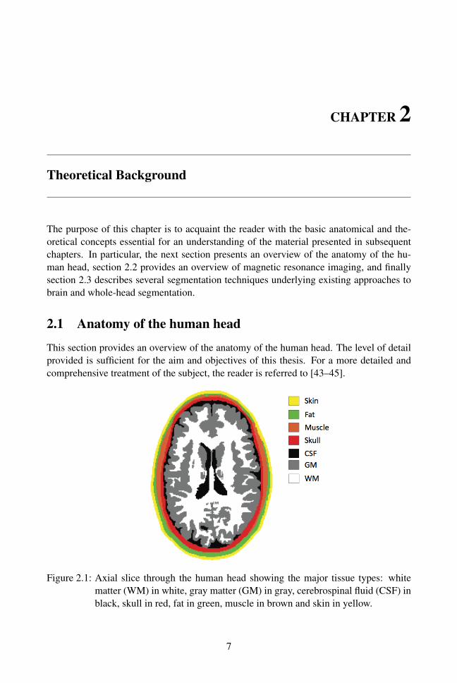
This section provides an overview of the anatomy of the human head. The level of detailprovided is sufficient for the aim and objectives of this thesis. For a more detailed andcomprehensive treatment of the subject, the reader is referred to [43–45].
Figure 2.1: Axial slice through the human head showing the major tissue types: whitematter (WM) in white, gray matter (GM) in gray, cerebrospinal fluid (CSF) inblack, skull in red, fat in green, muscle in brown and skin in yellow.
7

CHAPTER 2. THEORETICAL BACKGROUND
The human head is made up of numerous complex tissue types and structures [28].However it can be decomposed into the following major tissue types: white matter (WM),gray matter (GM), cerebrospinal fluid (CSF), skin, fat, muscle, and skull (as shown inFig. 2.1). These in turn can be classified as belonging to two major classes: brain andnon-brain.
2.1.1 Brain
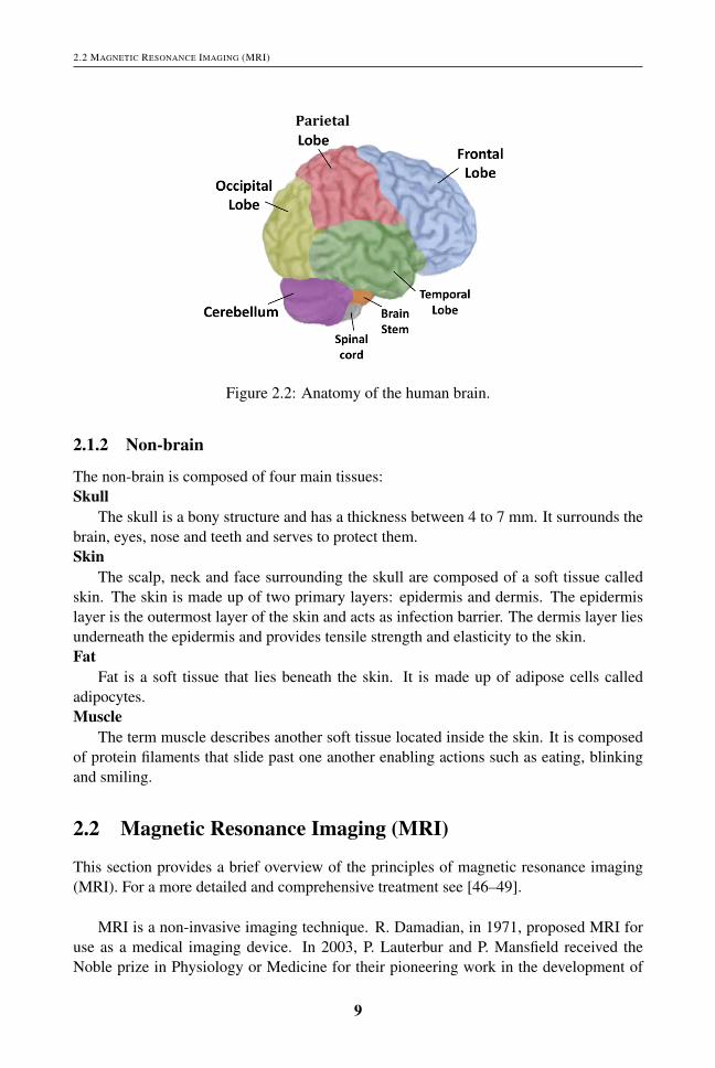
The human brain is an important part of the central nervous system. Functionally, it canbe decomposed into three main parts (see Fig. 2.2):
1. Cerebrum: This is the largest part of the brain and is composed of left and righthemispheres. Each hemisphere can in turn be divided into four lobes:
• Frontal Lobe: It is involved in functions such as reasoning, planning, parts ofspeech, voluntary motor function of skeletal muscles, emotions, and problemsolving.
• Parietal Lobe: It is involved in functions such as movement, orientation,recognition, and perception of stimuli.
• Occipital Lobe: It is involved in visual processing.
• Temporal Lobe: It is involved in functions such as perception and recognitionof auditory stimuli, memory, speech, and smell.
2. Cerebellum: It is located under the cerebrum and is involved in functions such asregulation and coordination of movement, posture, and balance.
3. Brain Stem: It is responsible for regulating breathing, heartbeat, and blood pressure.
Structurally, the brain can be decomposed into three main tissue types (shown in Fig.2.1):Gray matter
The gray matter is located on the thin outer layer of the brain, called the cerebralcortex, and also deeper in the brain underneath the white matter. It comprises neuronalcell bodies. Gray matter is involved in various functions including muscle control, speech,emotion, memory, vision and hearing.White matter
The white matter lies underneath the cerebral cortex and is made up of glial cells andbundles of myelinated axons. The white matter connects various regions of the gray mat-ter, favoring communication between cortical-cortical or cortical-subcortical structures.Cerebrospinal fluid (CSF)
The CSF is a colorless fluid. It is located in the subarachnoid space (space between thetwo protective membranes that surround the brain: arachnoid membrane and pia mater),the ventricles (large cavities inside the brain) and the spinal cord. It serves to protect thebrain, supply it with nutrition, and to remove waste.
8
2.2 MAGNETIC RESONANCE IMAGING (MRI)
!Parietal((
Figure 2.2: Anatomy of the human brain.
2.1.2 Non-brain
The non-brain is composed of four main tissues:Skull
The skull is a bony structure and has a thickness between 4 to 7 mm. It surrounds thebrain, eyes, nose and teeth and serves to protect them.Skin
The scalp, neck and face surrounding the skull are composed of a soft tissue calledskin. The skin is made up of two primary layers: epidermis and dermis. The epidermislayer is the outermost layer of the skin and acts as infection barrier. The dermis layer liesunderneath the epidermis and provides tensile strength and elasticity to the skin.Fat
Fat is a soft tissue that lies beneath the skin. It is made up of adipose cells calledadipocytes.Muscle
The term muscle describes another soft tissue located inside the skin. It is composedof protein filaments that slide past one another enabling actions such as eating, blinkingand smiling.
2.2 Magnetic Resonance Imaging (MRI)
This section provides a brief overview of the principles of magnetic resonance imaging(MRI). For a more detailed and comprehensive treatment see [46–49].
MRI is a non-invasive imaging technique. R. Damadian, in 1971, proposed MRI foruse as a medical imaging device. In 2003, P. Lauterbur and P. Mansfield received theNoble prize in Physiology or Medicine for their pioneering work in the development of
9

CHAPTER 2. THEORETICAL BACKGROUND
MRI.MRI is based on a physical phenomenon called nuclear magnetic resonance, which is
defined as the ability of magnetic nuclei to absorb energy from an electromagnetic pulseand to radiate this energy back. The hydrogen nucleus or proton is positively chargedand possesses an angular moment called spin. This property causes it to behave as a tinymagnet with a small magnetic field or magnetic moment.
In MR imaging the object to be imaged is placed inside a strong external magneticfield B0 that causes the protons either to align with B0 or opposed to it. The small dif-ference in the two populations yields a bulk magnetization M, which is the sum of theindividual magnetic moments of the individual protons, that depends linearly on the fieldintensity and is aligned with the B0 field (illustrated in Fig. 2.3). This state of magnetiza-tion is known as thermal equilibrium.
The magnetization vector M is the main source of the MR signal and is used to pro-duce an MR image. It has two components called longitudinal and transverse magnetiza-tion. The longitudinal magnetization (denoted as Mz) is parallel to the external magneticfield B0 while the transverse magnetization (denoted as Mxy) is perpendicular to the B0.
Figure 2.3: Alignment of protons with the B0 field: (a) with no external magnetic field,all the protons are oriented randomly (b) in the presence of external magneticfield (B0), some of the protons align with the field (parallel to the externalmagnetic field B0) whilst some of these oppose to the field (anti-parallel toB0). As a result, a net magnetization M = Mz is produced parallel to theexternal field B0. As a result, a net magnetization M=Mz is produced parallelto the external field B0 (adapted from [49]).
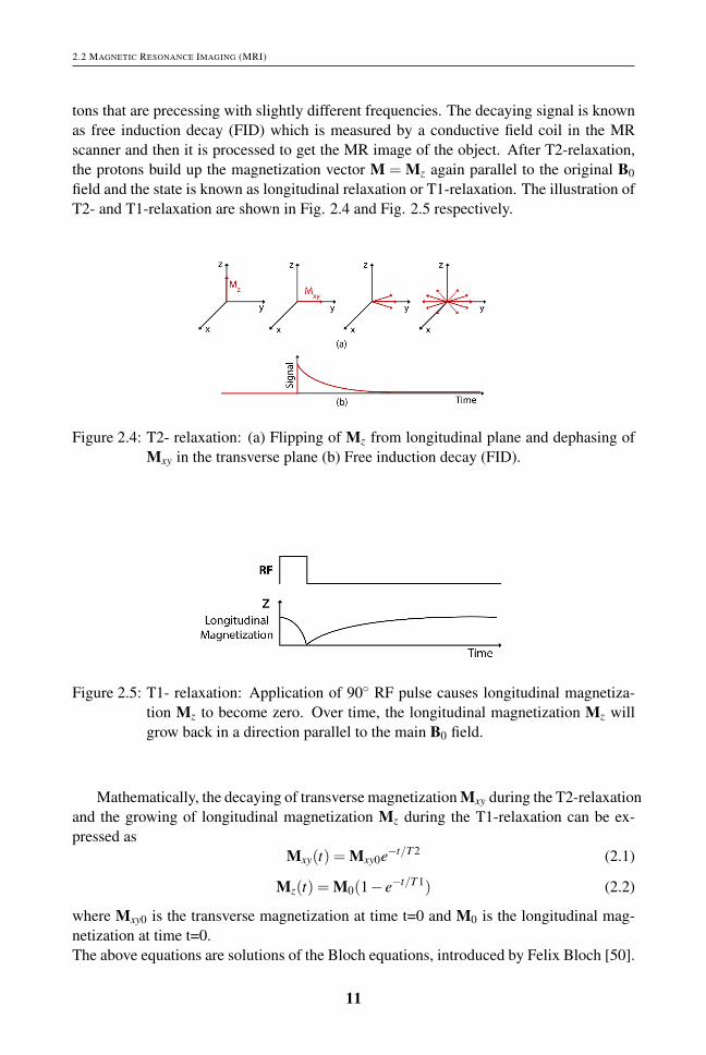
When a radio frequency (RF) pulse BRF (having frequency equal to the Larmor fre-quency) is applied, it gives energy to the protons. As a result, the magnetization vector Mflips in the transverse plane and the longitudinal component Mz becomes zero. Once theRF pulse is turned off, another RF signal is generated by the protons due to the magneticresonance phenomena. This signal is decaying towards zero when the magnetization vec-tor M = Mxy in the transverse plane starts to dephase. This state is known as transverserelaxation or T2-relaxation. The dephasing of Mxy is due to the magnetic moments of pro-
10
2.2 MAGNETIC RESONANCE IMAGING (MRI)
tons that are precessing with slightly different frequencies. The decaying signal is knownas free induction decay (FID) which is measured by a conductive field coil in the MRscanner and then it is processed to get the MR image of the object. After T2-relaxation,the protons build up the magnetization vector M = Mz again parallel to the original B0field and the state is known as longitudinal relaxation or T1-relaxation. The illustration ofT2- and T1-relaxation are shown in Fig. 2.4 and Fig. 2.5 respectively.
Figure 2.4: T2- relaxation: (a) Flipping of Mz from longitudinal plane and dephasing ofMxy in the transverse plane (b) Free induction decay (FID).
Figure 2.5: T1- relaxation: Application of 90◦ RF pulse causes longitudinal magnetiza-tion Mz to become zero. Over time, the longitudinal magnetization Mz willgrow back in a direction parallel to the main B0 field.
Mathematically, the decaying of transverse magnetization Mxy during the T2-relaxationand the growing of longitudinal magnetization Mz during the T1-relaxation can be ex-pressed as
Mxy(t) = Mxy0e−t/T 2 (2.1)
Mz(t) = M0(1− e−t/T 1) (2.2)
where Mxy0 is the transverse magnetization at time t=0 and M0 is the longitudinal mag-netization at time t=0.The above equations are solutions of the Bloch equations, introduced by Felix Bloch [50].
11

CHAPTER 2. THEORETICAL BACKGROUND
2D and 3D MR imaging
In MRI, two approaches called 2D and 3D imaging can be used to acquire a 3D imageof an object. In 2D imaging, the RF pulse is used to excite only the selected slice of anobject. In this way the signal generated from that particular slice is used to construct theimage of that slice. In 3D imaging, the volume of an object that contains the stack ofslices is excited with the RF pulse to get the image of that particular volume of an object.
2.2.1 Contrast Mechanisms in MRI
In MRI, the contrast between tissues is based on the intrinsic properties of the tissues;namely proton density (PD), T1 and T2.
T1 is defined as the time that it takes the longitudinal magnetization Mz to grow backto 63% of its original value. It is related to the rate of regrowth of longitudinal magnetiza-tion which is a fundamental source of contrast in T1-weighted images. Different tissueshave different rates of T1-relaxation, shown in Fig. 2.6.
T2 is defined as the time that it takes the transverse magnetization Mxy to decrease to37% of its starting value. It is related to the rate of dephasing of transverse magnetizationthat is a fundamental source of contrast in T2-weighted images. Different tissues havedifferent rates of T2-relaxation, shown in Fig. 2.7.
PD refers to the density of protons in the tissues. Different tissues have differentdensity of protons.
The weighting amount of T1 and T2 effects in the MR images, is controlled by twobasic scanning parameters known as echo time (TE) and repetition time (TR). TE is de-fined as the time between the start of the RF pulse and the maximum in the FID responsesignal. TR is defined as the time between the consecutive RF pulses.
The relative values of TE and TR to produce different contrast weighted images areshown in Fig. 2.8. A T1-weighted image is produced by maximizing the T1-relaxationand minimizing the T2-relaxation using short TE and intermediate TR. A T2-weightedimage is produced by maximizing the T2-relaxation and minimizing the T1-relaxationusing long TE and long TR. A PD-weighted image is produced by minimizing the bothT1- and T2-relaxation using short TE and long TR.
Figure 2.6: (a) T1: longitudinal magnetization increases to 63% of maximal Mz (b) Dif-ferent tissues have different rates of T1-relaxation.
12

2.2 MAGNETIC RESONANCE IMAGING (MRI)
Figure 2.7: (a) T2: transverse magnetization decreases to 37% of the starting value of Mxy
(b) Different tissues have different rates of T2-relaxation.
Figure 2.8: Scanning parameters: (a) short TE and intermediatory TR for T1-weighting(b) long TE and long TR for T2-weighting (c) short TE and long TR for PD-weighting.
Tissues of the human head visualized by magnetic resonance imaging
Fig. 2.9 shows three MR images of same axial slice through a human head. In these im-ages the contrast between soft tissues can be seen clearly. The contrast in these images arecharacterised as (a) T1-weighted (b) T2-weighted (c) PD-weighted. In the T1-weightedimage the CSF, skull, and fat appear dark and the gray matter, white matter, skin and
13

CHAPTER 2. THEORETICAL BACKGROUND
muscle appear bright. In the T2-weighted image the CSF and skin appear bright, and theskull, fat, muscle, white matter and gray matter appear darker than in the T1-weightedimage. In the PD-weighted image the fat, muscle, white matter, gray matter, and CSFappear bright, and the skull appears dark.
Figure 2.9: Axial slice from an MRI scan of the human head ( [51]) (a) T1-weighted (b)T2-weighted (c) PD-weighted image.
2.2.2 Basic pulse sequences for MRI
Two pulse sequences known as spin echo (SE) and gradient echo (GE) are commonlyused to generate MR images. These sequences are repeated many times during a scan togenerate the image of an object.
In a spin echo sequence, a 90◦ RF pulse is used to flip the magnetization vector M inthe transverse plane. As the protons go through the T1- and T2- relaxation, the transversemagnetization Mxy is gradually dephased. A 180◦ RF pulse is applied to rephase it. As aresult, a signal (called spin echo) is generated and is used to reconstruct an MR image. Inorder to generate the different contrast MR images, SE sequence is based on the TE andTR scanning parameters.
In gradient echo sequence, an RF pulse is applied that partly flips the net magneti-zation vector M into the transverse plane. A negative gradient pulse is used to dephasethe transverse magnetization Mxy and a positive gradient pulse is applied to rephase it.As a result, a signal (called gradient echo) is generated. In a GE sequence, the scanningparameters: flip angle, TE, and TR are used to produce different contrast MR images.However, in this thesis the MR images were acquired by applying the gradient echo pulsesequence.
2.2.3 Artifacts in MRI
The two major sources of artifacts that degrade MR image quality significantly and alsoobfuscate the anatomical and physiological detail are noise and the bias field. The noisein MRI is generally caused by the thermal agitation of electrons in the conductor. It isusually modeled as Rician distribution [52]. The bias field is a low frequency smoothundesirable signal which is caused by inhomogeneities in the magnetic field of the MRscanner. It changes the intensity values of the image pixels so that the same tissue hasdifferent gray level distribution across the image.
14
2.3 OVERVIEW OF THE BASIC SEGMENTATION TECHNIQUES UNDERLYING EXISTING APPROACHES TO BRAIN AND WHOLE-HEAD
SEGMENTATION
2.3 Overview of the basic segmentation techniques underlyingexisting approaches to brain and whole-head segmentation
Image segmentation refers to the process where every pixel in a digital image is assigneda label and such that pixels sharing the same characteristics are given the same label. Nu-merous techniques for image segmentation can be found in the literature [53]. No singletechnique is applicable for all problems and no general theory exists for synthesizing asegmentation solution for any given problem. The image analysis practitioner must there-fore devise solutions based on one or more techniques and using experience and trial anderror.In this section we give a brief description of the elementary segmentation techniques usedin the brain and whole-head segmentation methods presented/discussed in later chapters.
Mean Shift
Mean shift is a non-parametric mode seeking and clustering technique originally proposedby Fukunaga and Hostetler [54]. Its application to image processing and computer visiontasks such as filtering, image segmentation and real time object tracking was pioneeredby Comaniciu et al. [55].
Mean shift does not require any prior information concerning the number of clusters,and does not constrain the size or shape of the clusters. Mean shift clustering is based onan adaptive gradient ascent approach to estimate the local maxima or modes of multivari-ate distributions underlying the feature space. Ultimately each feature point is associatedwith a mode thereby defining clusters. The basic principle of mean shift clustering isdescribed below.
Let {xi ∈Rd |i = 1.....n} denote a set of feature vectors (data points) in d- dimensionalspace. The kernel density estimate of the underlying multivariate probability function atpoint x is given by
fK(x) =1n
n
∑i=1|H|−1/2K(|H|−1/2(x−xi)) (2.3)
where H is a d×d symmetric positive definite bandwidth matrix. For a radially symmetrickernel, H = h2I which leads to
fK(x) =ck,d
nhd
n
∑i=1
k
(∥∥∥∥x−xi
h
∥∥∥∥2)
(2.4)
where h > 0 is a scalar bandwidth and k : [0,1]→ R is the kernel profile of the radiallysymmetric kernel K with bounded support defined as
K(x) = ck,dk(‖x‖2
)‖x‖ ≤ 1 (2.5)
and ck,d is a normalizing constant ensuring that the kernel K integrates to 1. The typicalkernels used in the mean shift applications are Gaussian KG and Epanechnikov KE given
15
CHAPTER 2. THEORETICAL BACKGROUND
as
KG(x) = ck,dkG = ck,d exp(−1
2‖x‖2
)(2.6)
KE(x) = ck,dkE = ck,d(1−‖x‖2) ‖x‖ ≤ 1 (2.7)
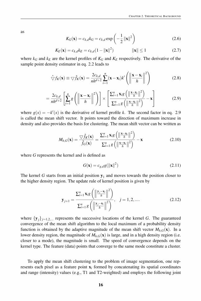
where kG and kE are the kernel profiles of KG and KE respectively. The derivative of thesample point density estimator in eq. 2.2 leads to
5 fK(x)≡5 fK(x) =2ck,d
nhd+2
n
∑i=1
(x−xi)k′(∥∥∥∥
x−xi
h
∥∥∥∥2)
(2.8)
=2ck,d
nhd+2
[n
∑i=1
g
(∥∥∥∥x−xi
h
∥∥∥∥2)]×
∑n
i=1 xig(∥∥x−xi
h
∥∥2)
∑ni=1 g
(∥∥x−xih
∥∥2) −x
(2.9)
where g(x) = −k′(x) is the derivative of kernel profile k. The second factor in eq. 2.9is called the mean shift vector. It points toward the direction of maximum increase indensity and also provides the basis for clustering. The mean shift vector can be written as
Mh,G(x) =5 fK(x)
fG(x)=
∑ni=1 xig
(∥∥x−xih
∥∥2)
∑ni=1 g
(∥∥x−xih
∥∥2) −x (2.10)
where G represents the kernel and is defined as
G(x) = cg,dg(‖x‖2) (2.11)
The kernel G starts from an initial position y1 and moves towards the position closer tothe higher density region. The update rule of kernel position is given by
y j+1 =
∑ni=1 xig
(∥∥∥y j−xi
h
∥∥∥2)
∑ni=1 g
(∥∥∥y j−xi
h
∥∥∥2) , j = 1,2, .... (2.12)
where {y j} j=1,2,... represents the successive locations of the kernel G. The guaranteedconvergence of the mean shift algorithm to the local maximum of a probability densityfunction is obtained by the adaptive magnitude of the mean shift vector Mh,G(x). In alower density region, the magnitude of Mh,G(x) is large, and in a high density region (i.e.closer to a mode), the magnitude is small. The speed of convergence depends on thekernel type. The feature (data) points that converge to the same mode constitute a cluster.
To apply the mean shift clustering to the problem of image segmentation, one rep-resents each pixel as a feature point xi formed by concatenating its spatial coordinatesand range (intensity) values (e.g., T1 and T2-weighted) and employs the following joint
16
2.3 OVERVIEW OF THE BASIC SEGMENTATION TECHNIQUES UNDERLYING EXISTING APPROACHES TO BRAIN AND WHOLE-HEAD
SEGMENTATION
spatial-range domain kernel Khs,hr(x) defined
Khs,hr(x) =C
hps hd
rk
(∥∥∥∥xs
hs
∥∥∥∥2)
k
(∥∥∥∥xr
hr
∥∥∥∥2)
(2.13)
where xs represents a vector of pixels spatial coordinates, xr represents a vector of pixelsrange (intensity) values and hs and hr are their corresponding kernel bandwidths and C isthe normalization constant.
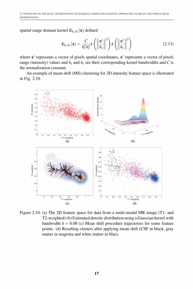
An example of mean shift (MS) clustering for 2D intensity feature space is illustratedin Fig. 2.10.
T1−weighted
T2
−w
eig
hte
d
T1−weighted
T2
−w
eig
hte
d
T1−weighted
T2
−w
eig
hte
dU
nn
orm
aliz
ed
de
nsity
T2−weightedT1−weighted
(b)(a)
(c) (d)
0 0.2 0.4 0.6 0.8 1
0
0.2
0.4
0.6
0.8
1
0 0.1 0.2 0.3 0.4 0.5 0.6 0.7 0.8 0.9 10
0.1
0.2
0.3
0.4
0.5
0.6
0.7
0.8
0.9
1
0 0.1 0.2 0.3 0.4 0.5 0.6 0.7 0.8 0.9 10
0.1
0.2
0.3
0.4
0.5
0.6
0.7
0.8
0.9
1
0
0.5
1
0
0.5
1
0
5
10
15
20
Figure 2.10: (a) The 2D feature space for data from a multi-modal MR image (T1- andT2-weighted) (b) Estimated density distribution using a Gaussian kernel withbandwidth h = 0.08 (c) Mean shift procedure trajectories for some featurepoints. (d) Resulting clusters after applying mean shift (CSF in black, graymatter in magenta and white matter in blue).
17

CHAPTER 2. THEORETICAL BACKGROUND
k-means Algorithm
The standard k-means algorithm was introduced by MacQueen [56,57] in 1967 to describeone of the simplest unsupervised clustering algorithms. In this algorithm, the partitioningof n data points into k disjoint subsets S j is done by minimizing the following cost function
J =k
∑j=1
∑i∈S j
‖xi−µ j‖2 (2.14)
where xi is a vector representing the ith data point and µ j is the centroid of the data pointsin S j.
The standard k-means algorithm starts with random initialization of k centroids. Eachdata point is then assigned to the closest centroid and the number of data points closest toa centroid form a cluster. The new centroid is computed according to the data points inthe cluster. This process is continued until the data points stop changing their centroidsor clusters. The downside of this algorithm is that it is quite sensitive to the initializationof the centroids of the clusters and it provides clustering in the intensity (range) domainonly.
Fuzzy c-means
Fuzzy c-means (FCM) was introduced by Dunn [58] and later improved by Bezdek [59].It aims to categorize each pixel in the image using fuzzy memberships.
Let {xi ∈Rd |i= 1.....N} represent an image with N pixels to be divided into c clusters.The FCM algorithm is an iterative optimization that minimizes the cost function given by
J =N
∑i=1
c
∑j=1
pmi j‖xi−µ j‖2. (2.15)
where pi j denotes the membership of pixel xi in the jth cluster, µ j is the jth cluster cen-ter, ‖.‖ is a norm metric, and m is a constant that controls the fuzziness of the resultingpartition.
The cost function is minimized when pixels close to the centroid of their clustersare assigned high membership values, and low membership values are assigned to pixelsfar from the centroid. The membership function represents the probability that a pixelbelongs to a specific cluster. The membership functions and cluster centers are updatedas follows
pi j =1
∑ck=1
( ‖xi−µ j‖‖xi−µk‖
) 2m−1
(2.16)
and
µ j =∑N
i=1 pmi jxi
∑Ni=1 pm
i j(2.17)
18

2.3 OVERVIEW OF THE BASIC SEGMENTATION TECHNIQUES UNDERLYING EXISTING APPROACHES TO BRAIN AND WHOLE-HEAD
SEGMENTATION
FCM starts with random initialization of c centroids and converges to a solution forµ j representing the local minimum of the cost function. The convergence is detected bycomparing the changes in the membership function or the cluster center at two sequentialiteration steps.
Parametric Statistical Methods
Parametric statistical methods assume some distributional form for the underlying prob-ability distribution of the image and seek to estimate its parameters. For example, theintensity of pixels in the image is typically modeled using a Gaussian mixture model(GMM) [60], which is a weighted sum of several component Gaussian densities. TheGMM is parameterized by the mean vectors, covariance matrices and mixture weightsfrom all component densities and these parameters are estimated using the Expectation-Maximization (EM) algorithm [61]. Finally, the segmentation is done by assigning everypixel to the class label for which it has the highest a posteriori probability.
The majority of methods that have been proposed in the literature for automated seg-mentation of brain tissues are based on parametric statistical models. For example, thehidden Markov random field model and associated Expectation-Maximization (HMRF-EM) algorithm is one of the state-of-the-art methods. In this algorithm, HMRF is astochastic model generated by a Markov random field (MRF) whose state sequence isestimated indirectly through observations. The advantage of HMRF is derived from theMRF theory in which the spatial information of an image is encoded through contex-tual constraints of neighbouring pixels. The EM algorithm is used to fit this model. Theprinciple of the HMRF-EM method is described below.
Let y = (y1, ........,yN) represent a gray-scale image such that yi represents the inten-sity of the i-th pixel. Let x = (x1, ........,xN) represent a label image such that xi ∈ L is thelabel corresponding to pixel yi and L is the set of all possible labels.
According to the maximum a posteriori (MAP) criterion, the optimal labeling x isobtained as follows
x = argmaxx{P(y|x,Θ)P(x)} (2.18)
where x is a realization of an MRF and P(x) is its prior probability given by
P(x) = Z−1 exp(−U(x)) (2.19)
where Z is a normalizing constant and U(x) is an energy function of the form
U(x) = ∑c∈C
Vc(x) (2.20)
where Vc(x) is the clique potential and C is the set of all possible cliques. In the image, aclique c is defined as a subset of pixels in which every pair of pixels are neighbors.P(y|x,Θ) represents the joint likelihood probability and is defined
19

CHAPTER 2. THEORETICAL BACKGROUND
P(y|x,Θ) = ∏i
P(yi|xi,θxi) (2.21)
where P(yi|xi,θxi) is a Gaussian distribution with parameters θxi = {µxiσxi}. Θ = {θl|l ∈L} is the set of parameters which are estimated using the EM algorithm. In [62], theiterated conditional modes (ICM) algorithm [63] (one of the optimization methods) isused to obtain the optimal solutions of MAP.
Four widely used brain tissue segmentation toolboxes: SPM (Statistical ParametricMapping toolbox) [64, 65], PVC (Partial Volume Classifier) [66], FreeSurfer [67] andFAST (FMRIB’s Automated Segmentation Tool) [62] are based on parametric statisticalmethods. For example, in SPM, the underlying method is based on the parameter esti-mations of a Gaussian mixture model (GMM), atlas registration and bias field correctionat the same time iteratively. In FreeSurfer, the underlying method includes registrationto a brain atlas, a Bayesian estimation theory framework, a Markov random field (MRF)spatial model and the ICM algorithm [63]. In PVC, the underlying method includes amaximum-a-posteriori (MAP) classifier and spatial prior model of the brain. In FAST, theunderlying method is based on the HMRF-EM algorithm.
20

CHAPTER 3
MRI Brain Tissue Segmentation
This chapter addresses objectives 1 and 2 of this thesis (described in chapter 1) for seg-menting the brain into three tissue types: white matter, gray matter and cerebrospinalfluid. The chapter consists of three sections. Section 3.1 presents a review of existingmethods for brain tissue segmentation. The proposed unsupervised framework is pre-sented in section 3.2. The empirical evaluation of the proposed method and the otherexisting unsupervised methods is presented in section 3.3.
3.1 MRI brain tissue segmentation methods: A review
Automated and accurate tissue segmentation is an important and challenging task in thequantitative analysis of brain MR images. In literature, a wide variety of automatic meth-ods have been proposed for segmenting the brain tissues in MR images. From the perspec-tive of machine learning, these can be broadly classified into two major types: supervisedand unsupervised segmentation methods.
Supervised segmentation methods [39, 68–72] need training datasets for feature ex-traction and classifier training. The trained classifier is then applied to label pixels inimage. However, supervised methods have a major drawback in that they require suf-ficiently large training dataset from a similar distribution as the data to be segmented.Consequently, in practice these methods are not suitable for data acquired with a differentscanner or scanning protocol [73].
In contrast, unsupervised methods don’t need any training datasets for segmentation.Various unsupervised methods have been proposed for brain tissue segmentation. Most ofthem are based on parametric statistical methods [18, 62, 64, 74–80], which assume somedistributional form for the underlying probability distribution of the data and seek to es-timate its parameters. Several of them [74–76] perform purely intensity based clustering.However, a major drawback of these is that they may give poor tissue classifications inthe presence of additive noise and multiplicative bias field inherent in MR images [41].To solve these problems, several parametric methods [18,62,64,77–79] employ a Markovrandom field (MRF) statistical spatial model. However, the main downside of these ap-proaches is that the MRF algorithm is computationally expensive and needs critical pa-rameter settings in a high dimensional feature space [41].
21

CHAPTER 3. MRI BRAIN TISSUE SEGMENTATION
Mean shift (MS) [54,55] is one of the unsupervised clustering methods, which doesn’thave this problem. It is an adaptive gradient approach to estimate the modes of the multi-variate distribution underlying the feature space. The feature points that have a commonmode constitute a cluster. The kernel bandwidth is the only parameter of the MS that in-fluences the clustering. For example, use of a small bandwidth can cause over-clusteringwhilst use of a large bandwidth can cause under-clustering. Numerous approaches [81,82]have been proposed to overcome this problem. These approaches employ adaptive band-width of the kernel to estimate the modes or clusters.
The mean shift based on the adaptive bandwidth for estimating the modes is calledthe adaptive mean shift (AMS) [81, 82]. AMS can perform clustering by taking boththe spatial and the intensity domain into account. This characteristic can make AMSmore robust to the MRI artifacts such as noise and spatial intensity inhomogeneity com-pared to intensity-based clustering methods [41]. AMS yields a set of clusters or modes.However, to get the desired number of clusters, merging is required. Mayer et al. [41]proposed the first adaptive mean shift framework for segmenting brain tissues in MR im-ages. This framework used a mode pruning and voxel-weighted k-means algorithm toassign the clusters, obtained from the adaptive mean shift, into white matter (WM), graymatter (GM) and cerebrospinal fluid (CSF) tissue. However, mode pruning in the range(intensity) domain ignores the spatial information of modes/clusters, which may causemerging of the modes belonging to different tissue types. In addition, merging of prunedmodes into desired tissue types using the voxel-weighted k-means algorithm, initializedby using prior knowledge of tissue intensity ordering in MR images [41], may also leadto assigning the clusters to the wrong tissue type. These collective limitations motivatedthe development of the new unsupervised segmentation framework presented in the nextsection.
3.2 Proposed unsupervised segmentation framework
We here propose a new unsupervised framework for segmenting the brain into three tissuetypes: WM, GM and CSF. The proposed framework is based on Bayesian adaptive meanshift, a priori spatial tissue probability maps and the fuzzy c-means algorithm
Bayesian adaptive mean shift is a variant of the AMS method proposed in [41]. InAMS, the adaptive bandwidth of the kernel is estimated in terms of the distance betweenthe current feature point and its k-th nearest neighbor. However, the estimation of thekernel bandwidth using this approach can be biased by outliers [83].
In [83] a fixed (global) kernel bandwidth estimation approach is proposed to solvethis problem. In the proposed framework, we employ this approach locally to estimate theadaptive bandwidth of the kernel for each feature point. The approach, called Bayesianadaptive mean-shift, uses a Bayesian method that involves fitting the Gamma distributionprobability density function to the local variances of N sets of neighborhoods around thecurrent feature point xi (for more details see [83] and appendix A in paper B).
22

3.2 PROPOSED UNSUPERVISED SEGMENTATION FRAMEWORK
Schematic of the proposed segmentation framework
A schematic of the proposed framework is presented in Fig. 3.1. The proposed frameworkinvolves three pre-processing steps: (1) Extraction of the brain from the MRI data (T1-weighted image) using a brain binary mask, obtained from the given ground truth. (2) Biasfield correction using the N3 bias field correction algorithm [84], and (3) Co-registrationof a priori spatial tissue probability maps, obtained from the ICBM [85], to the MRI braindata (T1-weighted brain image) using Flirt registration tool in FSL [86]. The followingsteps are then applied to segment the brain as follows:
1. Pre-clustering using Bayesian adaptive mean shift:
(a) The adaptive bandwidth hi for each feature point xi is estimated using theBayesian approach as described in paper B.
(b) The clusters of the brain tissue is then estimated, defined in Eq.2.12, using theadaptive bandwidth hi, obtained from step 1(a). The clustering is performedin the joint spatial-intensity domain using the joint kernel defined in Eq.2.13.
2. Final clustering to the desired number of clusters using fuzzy c-means: The fuzzyc-means algorithm (as described in section 2.3) is applied to assign the clusters,obtained from step 1(b), into the WM, GM, and CSF tissue using Eq.2.15. In thefuzzy c-means algorithm, the center of the jth tissue µ j is initialized by incorporat-ing the a priori spatial tissue probability maps pi j (obtained from the ICBM) usingEq.2.17.
Pre-processing ! Brain extraction ! Bias field correction
Bayesian adaptive mean shift
Image registration Fuzzy c-means
Input: T1-weighted image
T1-weighted brain image
Modes/Clusters
Output: WM, GM, CSF
a priori spatial tissue probability maps
Registered a priori spatial tissue probability maps
WM
GM
CSF
Figure 3.1: Schematic of the proposed framework.
23
CHAPTER 3. MRI BRAIN TISSUE SEGMENTATION
3.3 Empirical evaluation of the proposed framework
This section summarizes the empirical evaluation, detailed in paper B, of the proposedframework. The proposed framework was validated on a synthetic T1-weighted MR im-age with varying noise characteristics and spatial intensity inhomogeneity, obtained fromthe BrainWeb database as well as on 38 real T1-weighted MR images, obtained fromthe IBSR repository. The performance of the proposed framework was evaluated rela-tive to the three widely used brain segmentation toolboxes: FAST (FMRIBs AutomatedSegmentation Tool) [62], SPM (Statistical Parametric Mapping) [64, 65] and PVC (Par-tial Volume Classifier) [66], and the adaptive mean shift (AMS) [41] and classical Fuzzyc-means (FCM) [59] methods. The performance was evaluated both quantitatively andqualitatively.
Quantitative results
The quantitative performance of the proposed framework and each competing methodwas measured using the Dice index/score.
The Dice index/score (DI) [87] measures the degree of overlap between the groundtruth and the segmentation result. It is defined as
DI =2Vae
Va +Ve(3.1)
where Vae is the number of voxels the segmentation result and the ground truth have incommon, and Va and Ve denote the number of voxels in the segmentation result and theground truth respectively. The DI yields one for perfect overlapping and zero when thereis no overlap between the segmentation result and ground truth.
The quantitative results (mean Dice index) over all the subjects for the syntheticdataset and the IBSR18 dataset are presented in paper B; see figures 4, 5 and 7 respec-tively. Herein, we present in detail, the quantitative results for the IBSR20 dataset with20 subjects. The dataset was corrupted with strong intensity inhomogeneities (bias field).
The quantitative results for the IBSR20 dataset (shown in Fig. 3.2) show that acrossthe different subjects, for the GM, the proposed method yields higher or comparable seg-mentation accuracy (Dice index/score) for each subject compared to all competing meth-ods. However, for the WM, the proposed method has higher segmentation accuracy foreach subject compared to all competing methods except for the subjects 2 4, 15 3, 16 3for which SPM has higher segmentation accuracy, and the subject 2 4 for which FASTyields higher segmentation accuracy and the subject 191 3 for which FCM has highersegmentation accuracy. Moreover, for the CSF, the proposed method yields higher seg-mentation accuracy for each subject compared to all competing methods except for thesubject 202 3 for which SPM has higher segmentation accuracy and the subject 13 3 forwhich AMS has higher segmentation accuracy.
24

3.3 EMPIRICAL EVALUATION OF THE PROPOSED FRAMEWORK
!!!!!!!!!!!!!!!!!!
0.45
0.5
0.55
0.6
0.65
0.7
0.75
0.8
0.85
0.9
Subject (IBSR20)
Dic
e in
dex
1−
24 2−4
4−8
5−8
6−10 7−
88−
411−3
12−3
13−3
15−3
16−3
17−3
100−
2311
0−311
1−211
2−219
1−320
2−320
5−3
Proposed(WM)FAST(WM)AMS(WM)SPM(WM)PVC(WM)FCM(WM)
0.45
0.5
0.55
0.6
0.65
0.7
0.75
0.8
0.85
0.9
0.95
Subject (IBSR20)
Dic
e in
dex
1−
24 2−4
4−8
5−8
6−10 7−
88−
411−3
12−3
13−3
15−3
16−3
17−3
100−
2311
0−311
1−211
2−219
1−320
2−320
5−3
Proposed(GM)FAST(GM)AMS(GM)SPM(GM)PVC(GM)FCM(GM)
0
0.05
0.1
0.15
0.2
0.25
0.3
0.35
0.4
Subject (IBSR20)
Dice
inde
x
1−
242−
44−
85−
86−
107−
88−
411−
312−
3 13−
315−
316−
317−
3
100−23110−
3111−
2112−
2191−
3202−
3205−
3
Proposed(CSF)FAST(CSF)AMS(CSF)SPM(CSF)PVC(CSF)FCM(CSF)
(a) (b)
(c)
Figure 3.2: Dice index for each method for 20 subjects from the IBSR20 dataset for (a)WM (b) GM and (c) CSF.
However, over all the subjects, the quantitative results for the IBSR20 dataset (shownin Fig. 3.3) show that the proposed framework performs well (higher Dice index/score)for each tissue compared to all the competing methods. Moreover, the results for thecompeting methods, presented here are consistent with the results published in [88].
For the results shown in Fig. 3.2, several multiple comparison tests were done inorder to determine whether there exists a statistically significant difference in the voxel-wise classification performance between the proposed framework and each of the othermethods.
Each multiple comparison test involved performing five McNemar tests [89]. EachMcNemar test involved computing a 2×2 contingency matrix
[n11 n12n21 n22
](3.2)
where n11 is the number of voxels correctly classified by both methods, n12 is the numberof voxels correctly classified by proposed framework but not the other method, n21 is thenumber of voxels incorrectly classified by proposed framework but correctly classified bythe other method, and n22 is the number of voxels incorrectly classified by both methods.
For each McNemar test the null hypothesis was that the two methods have the sameperformance, i.e. n11 = n22, versus the alternative hypothesis that they do not. The levelof significance for each multiple comparison test was taken to be α=0.05 and so, usingBonferroni correction, the level of significance for each McNemar test was α =0.05/5
25

CHAPTER 3. MRI BRAIN TISSUE SEGMENTATION
=0.01.The McNemar tests for the IBSR20 dataset results for each tissue (shown in Fig. 3.2)
provide evidence that the proposed framework is significantly different (p-values < 0.01)to all competing methods.
!!!!!!!!!!!!!!!!!!
Proposed FAST AMS SPM PVC FCM 0.5
0.55
0.6
0.65
0.7
0.75
0.8
0.85
Dice
inde
x
Segmentation Methods
WM
Proposed FAST AMS SPM PVC FCM 0.5
0.55
0.6
0.65
0.7
0.75
0.8
0.85
0.9
Dice
inde
xSegmentation Methods
GM
Proposed FAST AMS SPM PVC FCM 0
0.05
0.1
0.15
0.2
0.25
Dice
inde
x
Segmentation Methods
CSF
(a) (b)
(c)
Figure 3.3: Mean Dice index for each method over the 20 subjects of the IBSR20 datasetfor (a) WM (b) GM and (c) CSF. The error bars show ±1 standard deviation.
Qualitative results
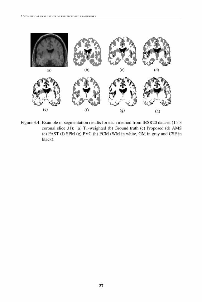
An illustration of segmentation for each method for coronal slice 31 of the subject 15 3from the IBSR20 dataset is presented in Fig. 3.4.
It can be seen that relative to the ground truth, the proposed framework has less mis-classification for the GM compared to all the competing methods. However, for the WM,the proposed framework has higher misclassification compared to SPM, especially in aregion close to the ventricles.
26
3.3 EMPIRICAL EVALUATION OF THE PROPOSED FRAMEWORK
!!!!!!!!!!!!!!!!!!!!!!!!!!!!!!!!!
(a) (b) (c) (d)
(e) (f) (g) (h)
Figure 3.4: Example of segmentation results for each method from IBSR20 dataset (15 3coronal slice 31): (a) T1-weighted (b) Ground truth (c) Proposed (d) AMS(e) FAST (f) SPM (g) PVC (h) FCM (WM in white, GM in gray and CSF inblack).
27

CHAPTER 3. MRI BRAIN TISSUE SEGMENTATION
28

CHAPTER 4
MRI Whole-Head Tissue Segmentation
This chapter addresses objectives 3 and 4 of this thesis described in chapter 1. It includesthree sections. Section 4.1 presents the motivation for developing an automated unsuper-vised method for whole-head segmentation. The proposed method is presented in section4.2. An evaluation of the segmentation accuracy of the proposed method is presented insection 4.3.
4.1 Automated head tissue segmentation: Motivation
Segmentation in MR head images can be useful for assigning individual tissues dielec-tric or biomechanical properties to construct a patient-specific dielectric or biomechanicalhead model, essential for electromagnetic or biomechanical simulations. Electromagneticmodeling is of importance in applications such as non-invasive EEG source localization inepilepsy patients [19], microwave imaging for stroke detection [20], hyperthermia treat-ment planning for head and neck tumors [21], the study of electric fields induced by tran-scranial magnetic stimulation (TMS) [22] and the study of deep brain simulation [23].Biomechanical modeling is of importance in applications such as brain deformation sim-ulation for image-guided neurosurgery [24] and the study of head trauma in traffic acci-dents [25].
The accuracy of the MR head tissues segmentation necessarily impacts on the qual-ity and fidelity of electromagnetic or biomechanical modeling. However, the accuratesegmentation of head tissues in MR images is a challenging task due to following majorreasons: (i) the complexity and variability of the underlying anatomy; (ii) noise; (iii) spa-tial intensity inhomogeneities; and (iv) the low contrast between the skull, CSF and air inconventionally-used T1-weighted images. This motivates to develop an accurate as wellas a fully automatic method for segmenting the head tissues in MR images, important foraccurate electromagnetic or biomechanical modeling.
4.2 Proposed whole-head segmentation method
Our proposed method is based on a hierarchical segmentation approach (HSA) incor-porating our novel Bayesian-based adaptive mean shift (BAMS) segmentation algorithm
29

CHAPTER 4. MRI WHOLE-HEAD TISSUE SEGMENTATION
(for more details see paper A). In common with several existing methods [19, 27, 32], theapproach includes first dividing the MRI data into brain tissue and non-brain tissue sub-volumes and then independently segmenting each of these into multiple tissue classes.The idea behind this HSA is that the detection of brain and non-brain tissue is a muchsimpler initial problem than the problem of segmenting the whole head into multiple tis-sue classes. For example the BET (Brain Extraction Tool, one of the state-of-the-art brainextraction tools) [90] can be employed to robustly obtain a brain-tissue mask whilst sim-ple thresholding and mathematical morphology operations [91, 92] can be employed toobtain a whole-head mask, from which the non-brain tissue mask can then be triviallyacquired. What differentiates our method is that a single segmentation approach, BAMS,is applied to segment both the brain tissue and non-brain tissue sub-volumes into multipletissue classes. The main advantage of BAMS is that it can make use of multiple MRImodalities such as T1-weighted, T2-weighted, and PD.
Hierarchical Segmentation Approach (HSA)
A schematic of the HSA is presented in Fig.4.1. The HSA takes as input a single MRimage (T1-weighted) or multi-modal MR images (T1-weighted, T2-weighted and PD) ofthe whole head. This data can be modeled as a single spatial volume (V ) with vector-valued voxels. In the first level of the HSA the T1-weighted data is employed to obtainboth a brain mask and a whole head mask. The BET tool is applied to obtain the formerand a simple whole head segmentation algorithm (WHSA) is used to obtain the latter. TheWHSA comprises two simple steps: (i) Otsu thresholding [91] and (ii) hole filling usingmorphological reconstruction and 26-connectivity [92]. The set difference between thesetwo masks then yields a mask of the non-brain head tissue. These masks effectively dividethe head volume (V ) into two disjoint sub-volumes: brain tissue (VBT ) and non-braintissue (VNBT ). In the second level of the HSA the multi-tissue segmentation algorithm(MTSA) is employed independently to the brain tissue (VBT ) and non-brain tissue (VNBT )volumes to segment them into individual tissue classes VBT1 , VBT2 ,...and VNBT1 , VNBT2 ,....respectively.
4.3 Empirical evaluation of the proposed method
This section summarizes the empirical evaluation, detailed in paper E, of the proposedmethod, HSA-BAMS. The evaluation was performed relative to a commonly used refer-ence method BET-FAST, and four instantiations of the HSA using both synthetic MRIdata (obtained from the Brainweb [51]) and real MRI data from ten subjects. EachHSA instantiation is based on a different multi-tissue segmentation algorithm: the hid-den Markov random field model and associated Expectation-Maximization (HMRF-EM)algorithm [62], the adaptive mean shift (AMS) algorithm [41], the improved Fuzzy c-means algorithm with spatial constraints (FCM S) [93], and the simple k-means cluster-ing algorithm [56]. Hereinafter these instantiations of the HSA are denoted HSA-FAST,HSA-AMS, HSA-FCM S and HSA-kmeans.
30

4.3 EMPIRICAL EVALUATION OF THE PROPOSED METHOD
!
!
!
PD
T2w
T1w
Non%brain!tissue!(!!"#)!
Brain!tissue!(!!")!
!!!"!! ,!!"!!,⋯!!
Head volume (V)#
BET
WHSA \
Multi-tissue segmentation algorithm (MTSA)
!!!! ,!!!!,⋯ !
Whole!head!mask
Brain!mask
Non%brain!mask
Multi-tissue segmentation algorithm (MTSA)
Figure 4.1: Schematic of the proposed hierarchical segmentation approach (HSA) for au-tomated whole head segmentation.
The synthetic data include multiple realizations of four different noise levels, andseveral realizations of typical noise with a 20% bias field level. For the synthetic MRIdata the ground truth was obtained from the nine tissue classes. This was reduced to sevenclasses by merging tissues with similar conductivity values. Notably, the connective andmuscle tissue classes were merged, and the glial matter and GM classes were merged.
For the real data sets, an experienced radio-oncologist manually segmented each sub-ject data into five tissue classes: WM, GM, CSF, skull and skin. This represented a trade-off between the time required to manually segment the images and labeling the essentialclasses for EEG source localization. The radio-oncologist included fat, muscle, and skin
31

CHAPTER 4. MRI WHOLE-HEAD TISSUE SEGMENTATION
in the skin class. The manual segmentation took about 170 hours for 200 slices.
Quantitative results
The quantitative performance of the proposed framework and that of each competingmethod was measured using the Dice index (defined in chapter 3) and the Hausdorff dis-tance [94], which is defined as
H = max{HSG,HGS} (4.1)
where S and G are two sets of points that belong to the segmentation result and groundtruth respectively. HSG = max{dSG
i } is the maximum value of the surface distance (Eu-clidian distance) of all surface voxels in S and dSG
i represents the minimum distance forthe ith surface voxel in S to the set of surface voxels in G. Similarly, HGS = max{dGS
i } isthe maximum value of the surface distance of all surface voxels in G and dGS
i representsthe minimum distance for the ith surface voxel in G to the set of surface voxels in S.
The quantitative results from paper E for the synthetic dataset with varying noisecharacteristics are shown in Fig. 2 and 3 respectively and the synthetic data for a particularnoise (5%) with 20% bias field is shown in Fig. 4. They show that the segmentationperformance of HSA-BAMS is consistently better (higher mean Dice index and lowermean Hausdorff distance) than that of all other instantiations of the HSA as well as thereference method BET-FAST for WM, GM, fat, and muscle tissue especially at highernoise levels (5%, 7%, and 9%). They also show that the segmentation accuracy of theproposed method is comparable (similar mean Dice index and mean Hausdorff distance)to the HSA-AMS and HSA-kmeans methods for the skin and skull tissue.
The quantitative results for the two real datasets (Data set 2 and Data set 3) for eachsubject are presented in Fig. 6 and 7 respectively. They show that the proposed methodHSA-BAMS yields higher segmentation accuracy (higher mean Dice index and lowermean Hausdorff distance) compared to all competing methods for the GM, skin, and skull.However, the performance of the proposed method is comparable (similar Dice index) toall competing methods for the WM (for Data set 2). Moreover, the methods BET-FASTand HSA-FAST have lower Hausdorff distance (H) compared to the proposed method forthe CSF (for Data set 3).
Herein, we present in detail, the quantitative results for the real dataset (Data set 4)with eight healthy subjects. The mean Dice index (DI) and mean Hausdorff distance (H)values over the eight subjects for each method and each tissue are shown in Fig. 4.2.They reveal that HSA-BAMS yields higher segmentation accuracy (higher mean Diceindex and lower mean Hausdorff distance) than the reference method BET-FAST as wellother variants of the HSA for all tissue types.
32

4.3 EMPIRICAL EVALUATION OF THE PROPOSED METHOD
!!!!!!!
HSA−BAMS HSA−AMS HSA−kmeans HSA−FAST BET−FAST HSA−FCM−S 0.65
0.7
0.75
0.8
0.85
0.9
Segmentation method(a)
Mean D
ice index
WMGMCSFSkinSkull
HSA−BAMS HSA−AMS HSA−kmeans HSA−FAST BET−FAST HSA−FCM−S 3
3.5
4
4.5
5
5.5
6
6.5
7
Segmentation method(b)
Mean H
ausdorf
f dis
tance (
mm
)
WMGMCSFSkinSkull
(a) (b)
Figure 4.2: Real Dataset: (a) Mean Dice index and (b) Mean Hausdorff distance (mm)over the eight subjects for each tissue and method. In (a) the error bars repre-sent±1 standard deviation of the Dice index and in (b) the error bars represent±1 standard deviation of the Hausdorff distance.
Qualitative results
An illustration of segmentation for each method for a single sagittal slice (the face re-gion has been excluded) of the subject (IXI040 Guys 0724 [95]) from the real datasetis shown in Fig. 4.3. It can be observed that for the skull tissue, HSA-kmeans, HSA-FCM S, HSA-FAST and HSA-AMS methods yield higher misclassification whilst for theskin tissue BET-FAST has higher misclassification. For the WM, all the competing meth-ods (HSA-kmeans, HSA-FCM S, HSA-FAST, HSA-AMS, and BET-FAST) yield highermisclassification compared to the proposed method HSA-BAMS.
33
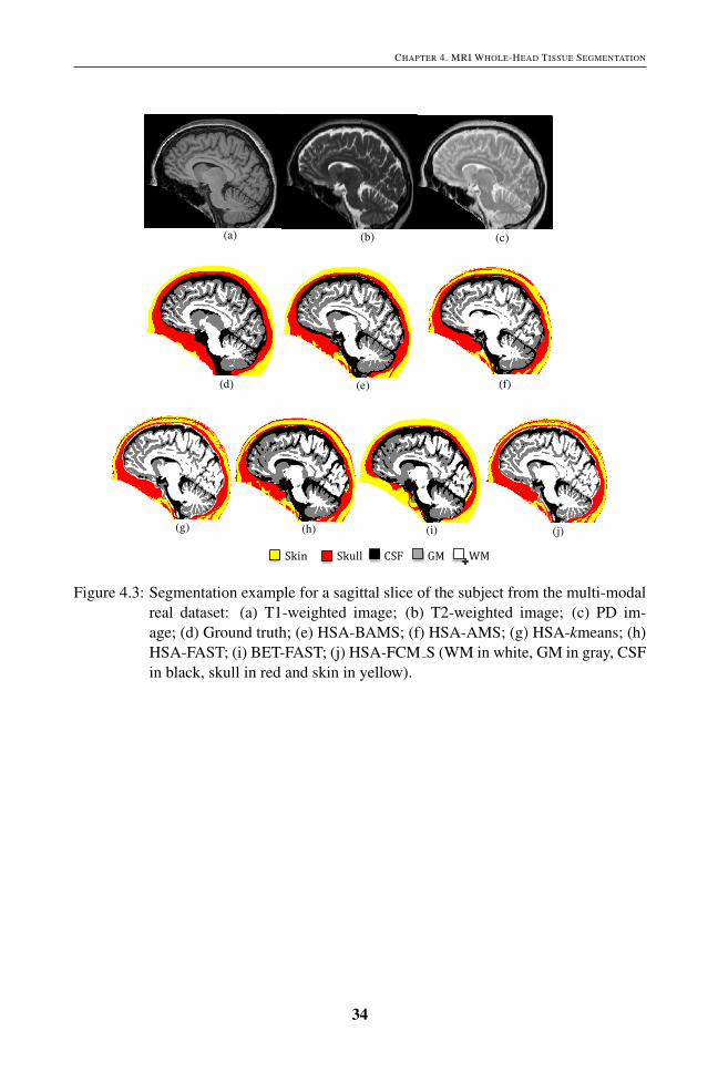
CHAPTER 4. MRI WHOLE-HEAD TISSUE SEGMENTATION
!
!
!
!
!
!
!
!
!
!
!
!
!
!
!
!
!
!
(a) (b) (c)
(d) (e) (f)
(g) (h) (j)
Skin!!!!!!!!!!!Skull!!!!!!!!CSF!!!!!!!!!GM!!!!!!!!!WM!
(i)
Figure 4.3: Segmentation example for a sagittal slice of the subject from the multi-modalreal dataset: (a) T1-weighted image; (b) T2-weighted image; (c) PD im-age; (d) Ground truth; (e) HSA-BAMS; (f) HSA-AMS; (g) HSA-kmeans; (h)HSA-FAST; (i) BET-FAST; (j) HSA-FCM S (WM in white, GM in gray, CSFin black, skull in red and skin in yellow).
34

CHAPTER 5
MRI Whole-Head Tissue Segmentation: Application to EEGSource Localization
This chapter addresses objective 5 of this thesis described in chapter 1. It includes threesections. Section 5.1 presents the motivation for developing an automated unsupervisedsegmentation method for electroencephalography (EEG) source localization. Section 5.2describes the EEG source localization problem. An evaluation of the proposed method,described in chapter 4, in the context of EEG source localization is presented in section5.3.
5.1 Automated head tissue segmentation for EEG source local-ization: Motivation
Epilepsy is one of the most common neurologic diseases, and is present in up to 1% ofthe world’s population. For epilepsy patients who have not been helped by medication,surgical therapy is often the only feasible intervention.
Source localization of epileptic activity is a tool to delineate cortical areas with abnor-mal neuronal activity of cells and networks. However, correct and anatomically preciselocalization of the epileptic focus is essential to decide if resection of brain tissue is pos-sible [96].
Expert manual analysis is considered the gold standard for determining accurate lo-calization of the source of epileptic seizures from electroencephalography (EEG) scalpmeasurements. Nevertheless, it is a time consuming and laborious process [96]. Sev-eral automatic non-invasive EEG source localization methods [97] have been proposedto solve this problem. The accuracy of these methods is not only based on the methodsapplied to solve the underlying forward and inverse problems [98] but also on the qualityand fidelity of the patient-specific head conductivity model used in the forward problem.The construction of a realistic head conductivity model needs accurate segmentation ofMR images of the head into tissue types corresponding to different conductivity values.It is usual practice to use five tissue classes: white matter, gray matter, CSF, skull, andskin [27, 99] followed by manual correction for source localization, although improve-ments in localization accuracy can be obtained with more tissue types [28]. Completely
35

CHAPTER 5. MRI WHOLE-HEAD TISSUE SEGMENTATION: APPLICATION TO EEG SOURCE LOCALIZATION
manual segmentation [26], normally performed by a clinical expert, is the gold standard.However, it is laborious and time-consuming. Two variations that can be found in the liter-ature are interactive segmentation/semi-automatic requiring user intervention [28–31,33],and fully automatic segmentation followed by manual correction [19, 27, 32]. Neverthe-less, these approaches are still labor intensive and time consuming. Additionally becauseuser interaction or intervention is needed they are, like completely manual segmentation,subjective and reproducibility is an issue.
Therefore, the limitations of semi-automatic and manual segmentation (outlined above)served as the motivation to develop a fully automatic method from multi-modal MR headimages suitable for EEG source localization.
5.2 The EEG Source Localization Problem
EEG source localization is a non-invasive tool applied to locate the source of epilepticseizures in the brain. It involves the solution of two problems: (1) Forward problemthat deals with finding the scalp potentials for the given current sources and (2) Inverseproblem that deals with estimating the sources to fit with the given potential distributionsat the scalp electrodes [27].
5.3 Evaluation of the proposed whole-head tissue segmenta-tion method: EEG source localization accuracy
The accuracy of EEG source localization is based on the quality and fidelity of the patient-specific head conductivity model, which is in turn based on the accuracy of segmentationof the patients head tissues.
Herein, we summarize an indirect empirical evaluation of our proposed segmentationmethod HSA-BAMS (described in chapter 4) in the context of EEG source localization,presented in paper E. The evaluation was performed relative to the ground truth (GT) andthe reference method BET-FAST using synthetic 2D multi-modal MR data with 3% noiselevel and synthetic EEG, generated for a prescribed source.
In addition, in paper C, the performance of BET-FAST (FSL software) was evaluatedrelative to the GT using the synthetic MRI data for 3% noise level with 20% bias field forthe EEG source localization. In paper D, the GT with five tissues was employed in orderto evaluate the modified particle swarm optimization method for EEG source localizationof somatosensory evoked potentials in a healthy subjects brain.
In paper E, a 2D GT with seven tissue types for the synthetic multi-modal MRI data,obtained from the BrainWeb, was used and a synthetic EEG was generated by placing asource in the GM of the GT image and calculating the EEG signals from 30 electrodesplaced equidistantly on the 2D scalp based on 10/10 system [27].
To solve the EEG source localization problems, a subtraction method was used formodeling the source (dipole) in the forward problem [100] and a modified particle swarmoptimization [27] method was applied to solve the inverse problem.
36
5.3 EVALUATION OF THE PROPOSED WHOLE-HEAD TISSUE SEGMENTATION METHOD: EEG SOURCE LOCALIZATION ACCURACY
Quantitative results
The performance of EEG source localization was measured in terms of relative error be-tween the measured and estimated source potential and localization error between theactual source and estimated source distance.The relative error (RE) is defined as
RE =‖Umeasured−Uestimated‖
‖Uestimated‖(5.1)
where Umeasured is a vector of the measured potential on the head and Uestimated is a vectorof the potential estimated using the simulated source.The localization error (LE) is defined as
LE = ‖Xtrue−Xestimated‖ (5.2)
where Xtrue is the real source position and Xestimated is the estimated source position.The quantitative results, presented in paper E, reveal that the relative error (RE) of the
potential and the localization error (LE) for the proposed method HSA-BAMS are 0.01and 0.00 mm respectively and for the reference method BET-FAST are 0.04 and 4.20 mmrespectively. It suggests that using HSA-BAMS leads to better localization accuracy.
Qualitative results
Herein, we discuss the qualitative results of each method, presented in paper E. Fig. 5.1shows the position of (a) real (simulated) source (in green) (b) estimated source using theproposed method HSA-BAMS (in red) (c) estimated source using the reference methodBET-FAST (in blue), superimposed on the ground truth image. It can be seen that theestimated position of the source obtained using HSA-BAMS is in good agreement withthe actual position of the source. However, the estimated position of the source obtainedusing the reference method BET-FAST is not.
37

CHAPTER 5. MRI WHOLE-HEAD TISSUE SEGMENTATION: APPLICATION TO EEG SOURCE LOCALIZATION
!
!
!
!
!
!
!
!
!
!
!
!
!
!
!
!
!
!
Figure10. EEG source localization results: Ground truth superimposed with the location of the real (simulated) source (green), HSA-BAMS estimated source (red), and BET-
FAST estimated source (blue).!
!
!!Skin!!!!!!Muscle!!!!!!!Fat!!!!!!!Skull!!!!!!CSF!!!!!!GM!!!!!!WM!
!Real!source!!!!!!!!!!Estimated!source!(HSA;BAMS)!!!!!!!Estimated!source!(BET;FAST)!
Figure 5.1: EEG source localization results: Ground truth superimposed with the locationof the real (simulated) source (green), HSA-BAMS estimated source (red),and BET-FAST estimated source (blue).
38

CHAPTER 6
MRI Whole-Head Tissue Segmentation: Application toHemorrhagic Stroke Detection
This chapter addresses objective 6 of this thesis described in chapter 1. It includes twosections. Section 6.1 presents the importance of microwave imaging for stroke detection,including image reconstruction procedure for intracerebral hemorrhage and an overviewof automated segmentation methods used for intracerebral detection. An evaluation ofsegmentation methods, including the proposed method described in chapter 4, in the con-text of intracerebral hemorrhage detection for a stroke patient is presented in section 6.2.
6.1 Application: Detecting Hemorrhagic Stroke with Microwave-Imaging
Stroke is a neurological disorder that is caused by either a clot blocking an artery or aburst blood vessel causing bleeding inside the cranium. The latter, called intracerebralhemorrhage, is the most common type [101]. Worldwide, each year approximately 15million people suffer a stroke. A third of these patients don’t survive [102].
Computerized Tomography (CT) is presently the gold standard for stroke diagnosis,with MRI frequently being applied when CT fails to give a definitive answer [103]. Themajor drawback of these imaging modalities is that they are rather bulky. Moreover,they are not portable. Thus, stroke patients have to be brought to the hospital to confirmthat they don’t have intracerebral hemorrhage before thrombolytic treatment, a treatmentemployed to dissolve blood clots in the brain, can be provided. Special, large ambulancesequipped with CT have been developed to address this problem [104]. Nevertheless, this isan expensive solution and can only be used in heavily populated areas with well developedtraffic and telecommunications infrastructure. Ultrasound is a potential future alternative.However, so far this is not applicable for detecting intracerebral hemorrhage [105]. Afast, cost-effective and portable stroke detection imaging system for ordinary ambulancesis thus highly desirable.
To achieve this, several microwave systems have been proposed/developed in recentyears [20, 35, 36, 106]. The microwave systems proposed in [20, 35, 36], have been usedfor numerical simulation for stroke detection while the one proposed in [106], has been
39
CHAPTER 6. MRI WHOLE-HEAD TISSUE SEGMENTATION: APPLICATION TO HEMORRHAGIC STROKE DETECTION
applied to clinical measurements from stroke patients.Microwave imaging uses several microwave antennas placed around the patient’s head
and measures the amplitude and phase for the propagated signal between all possible pairsof antenna combinations. A single frequency or multiple frequencies in an interval around1 GHz is often used. The dielectric properties of the brain tissues govern the microwavescattering [107]. The high contrast between blood and brain tissue facilitates the detec-tion of a hemorrhage. Microwave imaging is based on reconstructing dielectric imagesthat can be associated with physiological changes in the brain. To date, 3D reconstruc-tion algorithms typically require several hours for image reconstruction. However, thisis not feasible in ambulances where immediate reconstructions are required. It has beenproposed [36] that fast reconstruction can be obtained by exploiting a priori informationabout the patient’s brain in the healthy state (before stroke onset). In particular, a patient-specific dielectric model of the head is required as starting point; the reconstruction canthen be estimated as an update to the prior head model, wherein the measured signalsfrom the patient’s head are compared to the corresponding simulations of the head modeland changes in the tissue related to the stroke can be localized.
The quality and fidelity of the dielectric head model are essential for the accuracy ofimage reconstruction. However, the construction of a realistic dielectric head model in-volves, as a first step, the segmentation of the patient’s head tissues from MRI images. Thesegmentation can then be used to construct a dielectric head model by assigning each tis-sue type its respective dielectric property (conductivity/permittivity) value. Importantly,the accuracy of MRI tissue segmentation is critical for the construction of a realistic headmodel required for accurate image reconstruction.
6.1.1 Image reconstruction for intracerebral hemorrhage
Herein, we describe the image reconstruction procedure for intracerebral hemorrhage(shown in Fig. 6.1). The reconstruction involves the following steps:
1. Before the onset of stroke, a patient’s MRI data is segmented to generate a patient-specific dielectric head model. The model is then applied for electromagnetic sim-ulations to simulate the scattering parameters: transmission and reflection coeffi-cients (see Fig. 6.1, left).
2. After the onset of stroke, the electromagnetic measurements are performed directlyfrom the patient’s head using the microwave antennas surrounding the head (seeFig. 6.1, right).
3. Both measured and simulated scattering parameters are then used in the image re-construction algorithm, wherein the reconstruction is performed based on the differ-ence between the measured and simulated scattering parameters. The reconstruc-tion represents the change in dielectric properties of the brain tissues associatedwith intracerebral hemorrhage (see Fig. 6.1, center-bottom).
40

6.2 EVALUATION OF SEGMENTATION METHODS: INTRACEREBRAL HEMORRHAGE DETECTION
!
Patient dielectric head model (before stroke)
Electromagnetic simulation
Patient real head (after stroke)
Electromagnetic measurements
Simulated scattering parameters
Measured scattering parameters
Image reconstruction algorithm
Reconstructed intracerebral!hemorrhage
Figure 6.1: Schematic of image reconstruction for intracerebral hemorrhage.
6.2 Evaluation of segmentation methods: Intracerebral hem-orrhage detection
This section summarizes the empirical evaluation, detailed in paper F, of automated seg-mentation methods in the context of intracerebral hemorrhage detection for stroke patientusing microwave imaging system.
The evaluation was performed using both synthetic MRI data and real data from fourhealthy subjects. In the case of the synthetic data the labeled tissues used to generate theMRI data were served as ”ground truth” segmentation. In the case of the real data manualsegmentation done by an experienced radio-oncologist, was used as ”ground truth”. Thesegmentations were done on the full 3D data.
For computational reasons, in this study a 2D dielectric head model was used for elec-tromagnetic simulation and image reconstructions. The 2D model was constructed froma single 2D slice, obtained from the 3D segmented MRI data. Moreover, in this study, wemimic the scenario for real stroke measurements by using simulations of an intracerebralhemorrhage. The dielectric head model without intracerebral hemorrhage was generated
41
CHAPTER 6. MRI WHOLE-HEAD TISSUE SEGMENTATION: APPLICATION TO HEMORRHAGIC STROKE DETECTION
from each automated segmentation methods (described in section 6.2.1) while the headmodel with simulated intracerebral hemorrhage was generated only from the ground truth.The intracerebral hemorrhage was simulated in the head model by placing a disk of pre-scribed size in a prescribed position by assigning the pixels the dielectric properties forblood. Eight different hemorrhages were simulated: two different sized disks and fourdifferent positions. The radii for the large and small intracerebral hemorrhages were 20mm and 10 mm (see Fig. 3 in paper F).
The antenna configuration for the microwave imaging system, used in this study forelectromagnetic simulations is presented in Fig. 4 (see paper F). The imaging systemcomprises 20 antennas placed equidistantly around the dielectric head model. The an-tennas are used both as transmitters and receivers. For each tomographic measurement,one antenna at the time is used as transmitter while the others are used as receivers tomeasure the scattered signals. This process is continued until all antennas have been usedas transmitters and all possible antenna combinations have been measured.
The electromagnetic simulations for the head model without and with hemorrhagewere done independently by employing a 2D finite-difference time domain (FDTD) method[108, 109]. The FDTD method was used to simulate the electric fields inside the headmodel as well as to simulate the scattering parameters from the head model. The electricfields inside and the scattering parameters on the head model without hemorrhage, andthe measurements (measured scattering parameters) on the head model with hemorrhagewere then used as inputs to the image reconstruction algorithm in order to reconstruct theintracerebral hemorrhage (see Fig. 6.1).
In this study, we applied a fast reconstruction algorithm, which is based on a Bornapproximation [110] to find the difference between the simulated and measured signals,obtained from the head model without and with hemorrhage respectively, in order to deter-mine the change in dielectric properties of the brain tissues associated with intracerebralhemorrhage.
6.2.1 Automated segmentation methods
We used six unsupervised segmentation methods (including the proposed method pre-sented in chapter 4) for constructing the dielectric head model for use in simulated mi-crowave tomography system for imaging intracerebral hemorrhage for the stroke patients.The segmentation methods comprise the commonly used BET-FAST [62, 90] method,and five variations on a hierarchical segmentation approach (HSA) wherein the MRI datais initially divided into brain and non-brain and then the tissues are independently seg-mented in each. The detail of HSA is presented in section 4.2 and paper F respectively.Each HSA variant is based on a different multi-tissue segmentation algorithm: FAST [62],Bayesian-based adaptive mean shift (BAMS) [111], adaptive mean shift (AMS) [41], k-means method [56], Fuzzy c-means method [59]. These variants of the HSA are denotedHSA-FAST, HSA-BAMS (the proposed method presented in chapter 4), HSA-AMS,HSA-kmeans, and HSA-fuzzy cmeans.
42

6.2 EVALUATION OF SEGMENTATION METHODS: INTRACEREBRAL HEMORRHAGE DETECTION
Quantitative results
The quantitative evaluation included the measurement of segmentation accuracy over alltissues for a 2D slice, electromagnetic simulation accuracy, and image reconstruction ac-curacy for simulated intracerebral hemorrhage with two different sizes and four differentpositions in the brain.
The segmentation accuracy over all tissues, each method and each data was deter-mined in terms of mean Dice score/index [87].
The electromagnetic simulation accuracy was estimated in terms of signal deviation(F). The signal deviation was defined as the sum of squared difference between the scat-tering signals obtained from the dielectric models with and without intracerebral hemor-rhage, respectively. It is given by
F =N
∑k=1
n
∑t=1‖S′(k, t)−S(k, t)‖2 (6.1)
where N is the total number of antennas, n is the total number of signal samples and S′(k, t)
is the tth sample of the scattered signal received from the kth antenna, using the dielectrichead model with simulated intracerebral hemorrhage and S(k, t) is the tth sample of thescattered signal received from the kth antenna, using the dielectric head model withouthemorrhage.
The reconstructed image accuracy for both conductivity and permittivity of intracere-bral hemorrhage for each dataset and each method was estimated relative to the groundtruth in terms of relative error.
The relative error (RE) for the permittivity [108] is given by
RE =∑S ‖ξGT −ξASM‖
∑S ‖ξGT‖(6.2)
where S is the region of intracerebral hemorrhage being reconstructed, ξGT represents thepermittivity profile of the intracerebral hemorrhage reconstruction using the ground truth,and ξASM is the permittivity profile of the intracerebral hemorrhage reconstruction usingthe automatic segmentation method. The relative error for the conductivity is similarlydefined.
Moreover, the degree of overlap between the actual (simulated bleeding in the groundtruth brain) and reconstructed intracerebral hemorrhage was computed in terms of Dicescore for the image reconstruction accuracy.
The accuracy of electromagnetic microwave simulation is critical for the accurateimage reconstruction whilst the accuracy of segmentation is critical for the accurate elec-tromagnetic microwave simulation. In this study we investigated, how the segmentationaccuracy influences the electromagnetic microwave simulation accuracy. For this, a re-lationship between the segmentation accuracy and signal deviation (in logarithmic scale)was evaluated.
In paper F, Fig. 7 shows the combined plots for the mean Dice score over all the tissuesand the mean signal deviation over the four different positions for both large and small
43
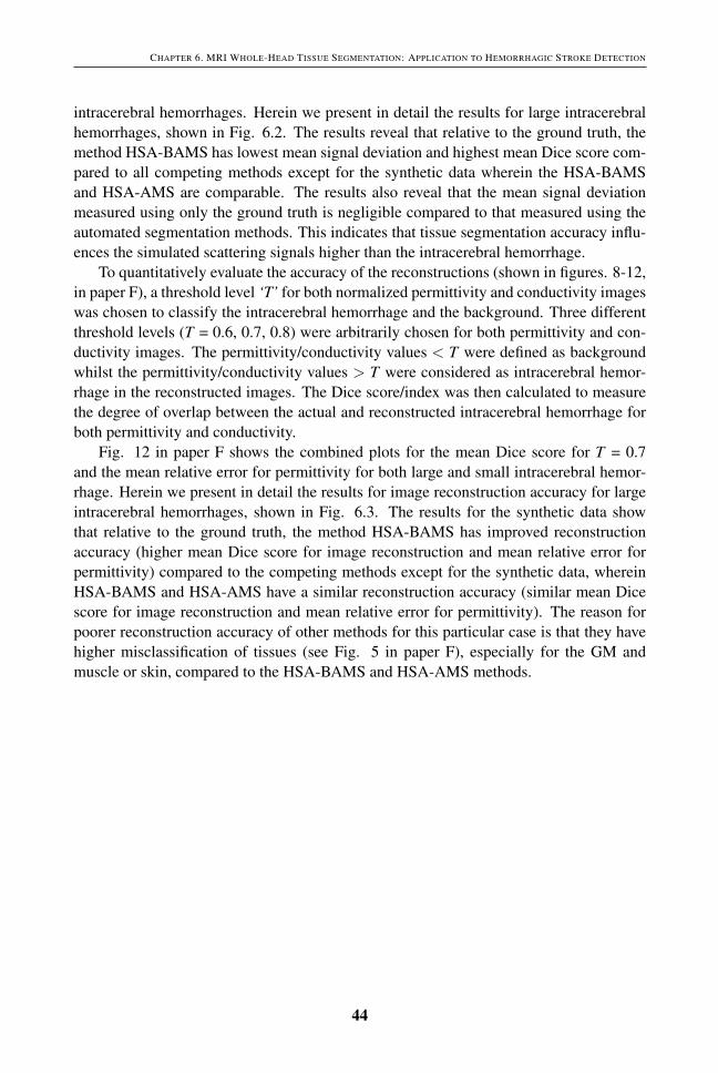
CHAPTER 6. MRI WHOLE-HEAD TISSUE SEGMENTATION: APPLICATION TO HEMORRHAGIC STROKE DETECTION
intracerebral hemorrhages. Herein we present in detail the results for large intracerebralhemorrhages, shown in Fig. 6.2. The results reveal that relative to the ground truth, themethod HSA-BAMS has lowest mean signal deviation and highest mean Dice score com-pared to all competing methods except for the synthetic data wherein the HSA-BAMSand HSA-AMS are comparable. The results also reveal that the mean signal deviationmeasured using only the ground truth is negligible compared to that measured using theautomated segmentation methods. This indicates that tissue segmentation accuracy influ-ences the simulated scattering signals higher than the intracerebral hemorrhage.
To quantitatively evaluate the accuracy of the reconstructions (shown in figures. 8-12,in paper F), a threshold level ‘T’ for both normalized permittivity and conductivity imageswas chosen to classify the intracerebral hemorrhage and the background. Three differentthreshold levels (T = 0.6, 0.7, 0.8) were arbitrarily chosen for both permittivity and con-ductivity images. The permittivity/conductivity values < T were defined as backgroundwhilst the permittivity/conductivity values > T were considered as intracerebral hemor-rhage in the reconstructed images. The Dice score/index was then calculated to measurethe degree of overlap between the actual and reconstructed intracerebral hemorrhage forboth permittivity and conductivity.
Fig. 12 in paper F shows the combined plots for the mean Dice score for T = 0.7and the mean relative error for permittivity for both large and small intracerebral hemor-rhage. Herein we present in detail the results for image reconstruction accuracy for largeintracerebral hemorrhages, shown in Fig. 6.3. The results for the synthetic data showthat relative to the ground truth, the method HSA-BAMS has improved reconstructionaccuracy (higher mean Dice score for image reconstruction and mean relative error forpermittivity) compared to the competing methods except for the synthetic data, whereinHSA-BAMS and HSA-AMS have a similar reconstruction accuracy (similar mean Dicescore for image reconstruction and mean relative error for permittivity). The reason forpoorer reconstruction accuracy of other methods for this particular case is that they havehigher misclassification of tissues (see Fig. 5 in paper F), especially for the GM andmuscle or skin, compared to the HSA-BAMS and HSA-AMS methods.
44
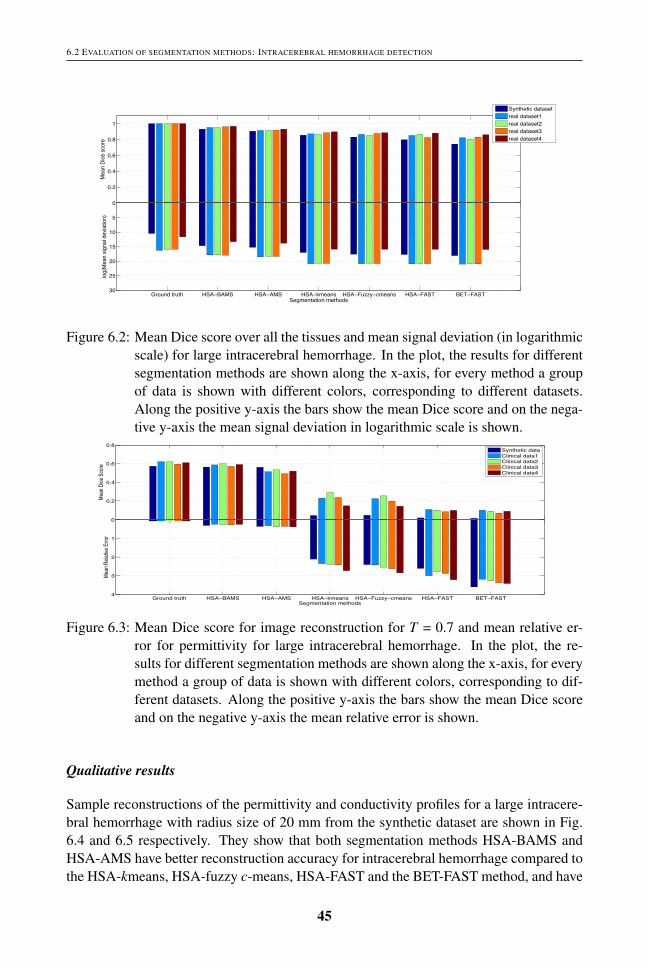
6.2 EVALUATION OF SEGMENTATION METHODS: INTRACEREBRAL HEMORRHAGE DETECTION
!
Ground truth HSA−BAMS HSA−AMS HSA−kmeans HSA−Fuzzy−cmeans HSA−FAST BET−FAST
0
5
10
15
20
25
30
log(
Mea
n sig
nal d
evia
tion)
Segmentation methods
0
0.2
0.4
0.6
0.8
1
Mea
n Di
ce s
core
Synthetic datasetreal dataset1real dataset2real dataset3real dataset4
Ground truth HSA−BAMS HSA−AMS HSA−kmeans HSA−Fuzzy−cmeans HSA−FAST BET−FAST
0
5
10
15
20
25
30
log(
Mea
n sig
nal d
evia
tion)
Segmentation methods
0
0.2
0.4
0.6
0.8
1
Mea
n Di
ce s
core
Synthetic datasetreal dataset1real dataset2real dataset3real dataset4
Figure 6.2: Mean Dice score over all the tissues and mean signal deviation (in logarithmicscale) for large intracerebral hemorrhage. In the plot, the results for differentsegmentation methods are shown along the x-axis, for every method a groupof data is shown with different colors, corresponding to different datasets.Along the positive y-axis the bars show the mean Dice score and on the nega-tive y-axis the mean signal deviation in logarithmic scale is shown.
!!
!!!!!!!
Ground truth HSA−BAMS HSA−AMS HSA−kmeans HSA−Fuzzy−cmeans HSA−FAST BET−FAST
0
1
2
3
4
Mean
Rela
tive E
rror
Segmentation methods
0
0.2
0.4
0.6
0.8
Mean
Dice
score
Synthetic dataClinical data1Clinical data2Clinical data3Clinical data4
Ground truth HSA−BAMS HSA−AMS HSA−kmeans HSA−Fuzzy−cmeans HSA−FAST BET−FAST
0
1
2
3
4
Mean
Rela
tive E
rror
Segmentation methods
0
0.2
0.4
0.6
0.8
Mean
Dice
Score
Synthetic dataClinical data1Clinical data2Clinical data3Clinical data4
Ground truth HSA−BAMS HSA−AMS HSA−kmeans HSA−Fuzzy−cmeans HSA−FAST BET−FAST
0
1
2
3
4
Mean
Rela
tive E
rror
Segmentation methods
0
0.2
0.4
0.6
0.8
Mean
Dice
Score
Synthetic dataClinical data1Clinical data2Clinical data3Clinical data4
Ground truth HSA−BAMS HSA−AMS HSA−kmeans HSA−Fuzzy−cmeans HSA−FAST BET−FAST
0
1
2
3
4
Mean
Rela
tive E
rror
Segmentation methods
0
0.2
0.4
0.6
0.8
Mean
Dice
score
Synthetic dataClinical data1Clinical data2Clinical data3Clinical data4Figure 6.3: Mean Dice score for image reconstruction for T = 0.7 and mean relative er-
ror for permittivity for large intracerebral hemorrhage. In the plot, the re-sults for different segmentation methods are shown along the x-axis, for everymethod a group of data is shown with different colors, corresponding to dif-ferent datasets. Along the positive y-axis the bars show the mean Dice scoreand on the negative y-axis the mean relative error is shown.
Qualitative results
Sample reconstructions of the permittivity and conductivity profiles for a large intracere-bral hemorrhage with radius size of 20 mm from the synthetic dataset are shown in Fig.6.4 and 6.5 respectively. They show that both segmentation methods HSA-BAMS andHSA-AMS have better reconstruction accuracy for intracerebral hemorrhage compared tothe HSA-kmeans, HSA-fuzzy c-means, HSA-FAST and the BET-FAST method, and have
45

CHAPTER 6. MRI WHOLE-HEAD TISSUE SEGMENTATION: APPLICATION TO HEMORRHAGIC STROKE DETECTION
a similar reconstruction accuracy compared to the ground truth. These results corroboratethe results for the synthetic data presented in Fig. 6.2. In the figures, the contours in thereconstructed images show the structures of the head tissues, wherein the actual intrac-erebral hemorrhage is shown as a circular contour. The color bar represents the rangeof intensity for the reconstructed images. In the reconstructed images, the white pixelscorrespond to background and the yellow and red pixels correspond to the intracerebralhemorrhage.
!
!
!!!!
(a) Ground truth (b) HSA-BAMS (c) HSA-AMS (d) HSA-kmeans (e) HSA-fuzzy c-means (f) HSA-FAST (g) BET-FAST
(a) Ground truth (b) HSA-BAMS (c) HSA-AMS (d) HSA-kmeans (e) HSA-fuzzy c-means (f) HSA-FAST (g) BET-FAST
Figure 6.4: Reconstruction of the permittivity profile for a large intracerebral hemorrhagewith radius size of 20 mm from the synthetic dataset obtained using the dif-ferent segmentation methods.
!
!
!!!!
(a) Ground truth (b) HSA-BAMS (c) HSA-AMS (d) HSA-kmeans (e) HSA-fuzzy c-means (f) HSA-FAST (g) BET-FAST
(a) Ground truth (b) HSA-BAMS (c) HSA-AMS (d) HSA-kmeans (e) HSA-fuzzy c-means (f) HSA-FAST (g) BET-FAST
Figure 6.5: Reconstruction of the conductivity profile for a large intracerebral hemorrhagewith radius size of 20 mm from the synthetic dataset obtained using the dif-ferent segmentation methods.
46

CHAPTER 7
Summary of the papers
This chapter presents brief summaries of the enclosed papers, which are categorized intothree types; brain segmentation, MRI whole-head segmentation for EEG source localiza-tion and MRI whole-head segmentation for intracerebral hemorrhage detection in strokepatients.
7.1 Brain Segmentation
7.1.1 Paper A: A Novel Bayesian Approach to Adaptive Mean Shift Seg-mentation of Brain Images
In this paper, we propose a novel adaptive mean shift algorithm for the segmentation ofmulti-modal MR images of the brain into three tissue types: white matter (WM), graymatter (GM) and cerebrospinal fluid (CSF). The novelty lies in the algorithm for the esti-mation of adaptive bandwidth of the kernel. The algorithm is called a Bayesian adaptivemean shift (BAMS) wherein the Bayesian approach is employed for adaptive bandwidthestimation. The approach involves fitting the Gamma distribution probability densityfunction to the local variances of N sets of neighborhoods around the current featurepoint. The accuracy of the proposed algorithm BAMS was evaluated relative to anotheradaptive mean shift algorithm that is based on the k nearest neighbors (kNN) bandwidthestimator as well as several other existing methods. The segmentation experiments wereperformed on both multi-modal synthetic (T1-, T2-, PD-weighted) MRI data with differ-ent levels of noise and real T1-weighted MRI data with varying levels of spatial intensityinhomogeneities. The performance of the segmentation methods was measured using theDice and Tanimoto coefficient. The results demonstrate the efficacy and accuracy of theproposed BAMS algorithm and that it performs well compared to the competing methodsespecially when the noise and spatial intensity inhomogeneities are high.
47
CHAPTER 7. SUMMARY OF THE PAPERS
7.1.2 Paper B: Automated MRI Brain Tissue Segmentation based on MeanShift and Fuzzy C-Means using a Priori Tissue Probability Maps
In this paper, we propose a novel fully automatic unsupervised segmentation frameworkfor the segmentation of three tissue types from the MRI brain images. The frameworkis based on the Bayesian-based adaptive mean shift to initially divide the brain into anumber of clusters and the fuzzy c-means algorithm, wherein the a priori spatial tissueprobability maps are incorporated, to classify the resulting clusters into WM, GM andCSF tissue. The segmentation accuracy of the proposed framework was evaluated rela-tive to three widely used brain segmentation toolboxes: FAST, SPM, and PVC and theadaptive mean shift (AMS) and classical fuzzy c-means (FCM) methods. The evaluationwas done on a synthetic T1-weighted MR image for four different noise levels (3%, 5%,7%, 9%) with two different spatial intensity inhomogeneity levels (20%, 40%), obtainedfrom the BrainWeb database as well as on 38 real T1-weighted MR images, obtainedfrom the IBSR repository. The experimental results, especially for the real datasets revealthat for some cases, the proposed framework has less segmentation accuracy for sometissue compared to the competing methods. However, overall the performance of the pro-posed framework is better compared to all competing methods. Moreover, incorporationof a priori spatial tissue probability maps in the proposed framework makes the tissuesegmentation objective and reproducible.
7.2 MRI Whole-Head Segmentation: EEG Source Localiza-tion
7.2.1 Paper C: Investigation of Brain Tissue Segmentation Error and ItsEffect on EEG Source Localization
In this paper, the segmentation performance of two widely used brain segmentation tools:FSL (FAST) and FreeSurfer were evaluated relative to the ground truth (gold standardsegmentation). The evaluation was performed using the synthetic MRI data with varyingnoise and bias field levels, obtained from the BrainWeb. The segmentation results showthat FSL is more robust compared to FreeSurfer, especially for the CSF, one of the mostimportant tissues for EEG source localization. Based on the FSL segmentation, an electro-conductivity head model was then constructed in order to investigate the effects of braintissue segmentation on EEG source localization. A combination of the subtraction methodand modified particle swarm optimization method was applied to solve the EEG sourcelocalization problems. The experimental results show that the source estimated using theFSL based electro-conductivity model has a 12 mm localization error in the z-direction ofthe estimated source.
48

7.2 MRI WHOLE-HEAD SEGMENTATION: EEG SOURCE LOCALIZATION
7.2.2 Paper D: Particle Swarm Optimization Applied to EEG Source Lo-calization of Somatosensory Evoked Potentials
In this paper, a modified particle swarm optimization method was applied for EEG sourcelocalization of somatosensory evoked potentials in a healthy subject’s brain. This pa-per provides an extension of the work presented in paper C, wherein it is shown that thewidely used brain segmentation tool: FSL has high misclassifications of skull and CSFtissue. This might cause significant errors in source localization results. Herein, man-ual segmentation of T1-weighted MRI data of the healthy subject, done by a radiologist,was employed. The segmentation was then applied to construct a conductivity model forsource localization of somatosensory evoked potentials. The experimental results showthat using the expert manual segmentation of tissues, the modified particle swarm opti-mization method yields the accurate source localization of somatosensory evoked poten-tials in the healthy subject’s brain with respect to the clinical expert determined sourcelocalization as well as to the exhaustive search source localization method.
7.2.3 Paper E: Unsupervised Segmentation of Head Tissues from Multi-modal MR Images for EEG Source Localization
In this paper, we propose and present a new fully automatic unsupervised method for headtissue segmentation from multi-modal MR images for use in the construction of a patientspecific model for EEG source localization. The method is based on a hierarchical seg-mentation approach (HSA), wherein the MRI data are initially divided into brain tissueand non-brain tissue sub-volumes and then each sub-volume is independently segmentedinto multiple tissue classes. What differentiates our method is that a single segmentationapproach, Bayesian adaptive mean shift (BAMS), is used to segment both the brain tissueand non-brain tissue sub-volumes into multiple tissue classes. Several evaluations of theperformance of the proposed method and of reference as well as variant methods were alsopresented. This included direct evaluation in terms of segmentation accuracy and indirectevaluation in terms of EEG source localization accuracy. The segmentation results showthat compared to the competing methods, the proposed method is more tolerant to thenoise and the bias field for the synthetic data. For the real datasets, the proposed methodalso has higher segmentation accuracy for the tissue types essential for the EEG sourcelocalization compared to each competing method. Moreover, multiple comparisons sta-tistical tests (consisting of several McNemar tests) also show that the proposed methodHSA-BAMS performs differently (p-values < 0.016) to all other methods for each tis-sue type, especially for the real datasets. For the case of EEG source localization, theresults show that the proposed method yields a better performance compared to the ref-erence method BET-FAST, commonly used for the construction of a realistic head modelfor EEG source localization. Overall the experimental results suggest that the proposedmethod HSA-BAMS can be used as a surrogate for the reference method BET-FAST aswell as manual segmentation for the construction of patient-specific head models for EEGsource localization.
49

CHAPTER 7. SUMMARY OF THE PAPERS
7.3 MRI Whole-Head Segmentation: Intracerebral HemorrhageDetection in Stroke Patients
7.3.1 Paper F: A Comparative Study of Automated Segmentation Methodsfor Use in a Microwave Tomography System for Imaging Intracere-bral Hemorrhage in Stroke Patients
In this paper, we present an evaluation of several unsupervised segmentation methods inthe context of intracerebral hemorrhage detection in stroke patients using a microwaveimaging system. The evaluation was performed using both synthetic MRI data and realdata from four healthy subjects. In the case of the synthetic data the labeled tissues usedto generate the MRI data were used as ”ground truth” segmentation. In the case of the realdata expert manual segmentation was served as ”ground truth”. The segmentations weredone on the full 3D data, whereas the electromagnetic evaluation was performed using a2D slice. For evaluation of methods, we calculated the segmentation accuracy over the tis-sues relative to the ground truth. We also evaluated the effect caused by misclassificationof tissue on the electromagnetic wave propagation through the head and on the recon-struction accuracy of hemorrhage. The segmentation accuracy was measured in terms ofthe degree of overlap (Dice score) between the ground truth and the method segmenta-tion. The electromagnetic simulation accuracy was measured in terms of signal deviationrelative to the simulation based on the ground truth. Finally, the image reconstructionaccuracy was measured in terms of the Dice score, the relative error of dielectric proper-ties, and visual assessment between true and reconstructed intracerebral hemorrhage. Theexperimental results reveal that accurate image reconstruction for the intracerebral hem-orrhage in the subject’s brain can be achieved by accurate segmentation of tissues in theMRI data. They also indicate that accurate automated segmentation (in this study, partic-ularly HSA-BAMS) can be applied in lieu of manual segmentation and can assist in fastdiagnosing the intracerebral hemorrhage in stroke patients using the microwave imagingsystem.
50

CHAPTER 8
Conclusions and Outlook
In this chapter our contributions are summarized and directions for future work are dis-cussed.
8.1 Conclusions
The contributions of this thesis are four-fold. First, we studied the brain segmentationproblem for three tissue types: WM, GM and CSF in MR images, wherein accurate seg-mentation is a challenging task because of the two major artifacts: noise and spatial inten-sity inhomogeneity (bias field). In chapter 3, we presented an unsupervised segmentationframework, which is a combination of Bayesian adaptive mean shift, a priori spatial tis-sues probability maps and the fuzzy c-means algorithm. The important characteristic ofthe proposed framework is that it provides the segmentation of tissue by taking both thespatial and intensity domain and the a priori spatial information using probabilistic atlasinto account. This makes the proposed method more robust to noise and spatial intensityinhomogeneity. Overall the experimental results showed that the proposed frameworkexhibited a higher degree of segmentation accuracy in segmenting both synthetic and 38real T1-weighted MR images compared to the competing methods. However, over all thesubjects for each real dataset, the proposed framework has decreased in performance forthe CSF compared to the WM and GM.
Second, we studied the whole-head segmentation problem in the multi-modal MRimages for use in the construction of a patient specific dielectric model. In chapter 4, weproposed an automated unsupervised MRI whole-head tissue segmentation method foruse in biomechanical or electromagnetic modeling. The method is based on a hierarchi-cal segmentation approach (HSA) incorporating the Bayesian-based adaptive mean-shift(BAMS), wherein the MRI data is first partitioned into brain tissue and non-brain tissuesub-volumes and then each sub-volume is independently segmented.
Third, we studied the influence of MRI head tissue segmentation on the accuracyof EEG source localization. In chapter 5, the proposed whole-head tissue segmentationmethod HSA-BAMS is evaluated for the EEG source localization. The experimental re-sults demonstrated the accuracy of the proposed method, and that it is more suitable thanthe reference method BET-FAST commonly used for constructing the realistic head con-
51

CHAPTER 8. CONCLUSIONS AND OUTLOOK
ductivity model for EEG source localization.Fourth, we studied the influence of MRI head tissue segmentation on the accuracy
of image reconstruction for intracerebral hemorrhage detection in stroke patients usinga microwave imaging system. In chapter 6, we presented an evaluation of the proposedwhole-head tissue segmentation method HSA-BAMS for use in constructing a dielectrichead model for imaging intracerebral hemorrhage in stroke patients using a simulatedmicrowave imaging system. The experimental results demonstrated that the proposedmethod yields a higher image reconstruction accuracy for intracerebral hemorrhage com-pared to the existing methods. The results also revealed that accurate automated segmen-tation can be used in lieu of manual segmentation for accurate image reconstruction andcan assist in real time stroke detection in the patient’s brain using the microwave imagingsystem.
8.2 Future work
Based on the studies presented in this thesis, the following possibilities can be exploredin future research.
• The proposed framework for brain segmentation, presented in chapter 3, can be ap-plied for segmenting MR images containing abnormal brain tissues like scleroticlesions and tumors. This will likely require additional MRI modalities and possi-bly also imaging modalities. These can be readily accommodated in the proposedmethod.
• The robustness of the proposed method, presented in chapter 4, can be investi-gated for real time diagnosis of stroke patients in the ambulance equipped with amicrowave imaging system.
• The proposed method, presented in chapter 4, can also be investigated for hyper-thermia treatment planning for head and neck tumors, wherein the accurate seg-mentation for tumors and tissues surrounding the tumors are crucial for accuratetreatment.
• The proposed framework, presented in chapter 3, can be investigated for simulta-neous tissue segmentation and bias field estimation of MR images. This can beachieved by extending the fuzzy c-means objective function (Eq.2.15) for bias fieldestimation [112].
• T1- and T2-weighted MR images contain low contrast between the air and the skulltissue, which may cause misclassification of the skull. One potential solution to thisproblem is to incorporate a priori anatomical information; e.g. using a probabilisticatlas. This can be investigated for the proposed method, presented in chapter 4.
• It can also be possible to investigate other contemporary segmentation techniquessuch as multi-atlas segmentation methods for EEG source localization and stroke
52

8.2 FUTURE WORK
detection in the patient’s brain. Multi-atlas yields a better tissue segmentation forthe brain datasets with large anatomical variations than a single atlas [113].
53

CHAPTER 8. CONCLUSIONS AND OUTLOOK
54

Bibliography
[1] O. F. Erondu. Medical Imaging. InTech, 2011.
[2] W. R. Hendee and E. R. Ritenour. Medical Imaging Physics. Wiley-Liss, 2002.
[3] C. Guy and D. Ffytche. An Introduction to The Principles of Medical Imaging.Imperial College Press, 2008.
[4] B. L. Hart, E. C. Benzel, and C. C. Ford. Fundamentals of Neuroimaging. W. B.Saunders, 1997.
[5] B. Husing, L. Jancke, and B. Tag. Impact Assessment of Neuroimaging. Institutefor Biomedical Engineering, University of Zurich and ETHZ, Zurich, Switzerland,2005.
[6] B. Crosson, A. Ford, K. M. McGregor, M. Meinzer, S. Cheshkov, X. Li, D. Walker-Batson, and R. W. Briggs. Functional imaging and related techniques: An intro-duction for rehabilitation researchers. J. Rehabil. Res. Dev., 47(2):vii–xxxiv, 2010.
[7] D. L. Bailey, D. W. Townsend, P. E. Valk, and M. N. Maisey. Positron EmissionTomography: Basic Sciences. Secaucus, NJ: Springer-Verlag, 2005.
[8] S. A. Huettel, A. W. Song, and G. McCarthy. Functional Magnetic ResonanceImaging. Massachusetts: Sinauer, 2nd edition, 2009.
[9] E. S. Schwartz, D. J. Dlugos, P. B. Storm, J. Dell, R. Magee, T. P. Flynn, D. M.Zarnow, R. A. Zimmerman, and T. P. Roberts. Magnetoencephalography for pedi-atric epilepsy: how we do it. American Journal of Neuroradiology, 29(5):832–837,2008.
[10] E. B. Swartz. The advantages of digital over analog recording techniques. Elec-troencephalography and Clinical Neurophysiology, 106(2):113–7, 1998.
[11] G. W. Small. Chapter 86: Structural and functional brain imaging of Alzheimerdisease, Neuropsychopharmacology: The Fifth Generation of Progress. LippincottWilliams Wilkins, 2002.
[12] G. T. Herman. Fundamentals of computerized tomography: Image reconstructionfrom projection. Springer, 2009.
[13] J. B. Jr Ball and M. L. Pensak. Fundamentals of Magnetic Resonance Imaging.American Journal of Otolaryngology, 8:81–85, 1987.
55

BIBLIOGRAPHY
[14] G. Zhai, W. Lin, K. Wilber, G. Gerig, and J. H. Gilmore. Comparison of regionalwhite matter diffusion in healthy neonates and adults using a 3T head-only MRscanner. Radiology, 229:673–681, 2003.
[15] J. Gilmore, G. Zhai, K. Wilber, J. Smith, and W. Lin. 3T magnetic resonanceimaging of the brain in newborns. Psychiatry Research Neuroimaging, 132:81–85,2004.
[16] W. Minjie. Registration and segmentation of brain MR images from elderly indi-viduals. PhD thesis, University of Pittsburgh, 2009.
[17] X. Han and B. Fischl. Atlas renormalization for improved brain MR image seg-mentation across scanner platforms. IEEE Trans. Med. Imaging, 26(4):479–486,2007.
[18] H. Greenspan, A. Ruf, and J. Goldberger. Constrained Gaussian mixture modelframework for automatic segmentation of MR brain images. IEEE Trans. Med.Imaging, 25(9):1233–1245, 2006.
[19] M. Rullmann, A. Anwander, M. Dannhauer, S. Warfield, F. Duffy, and C. Wolter.EEG source analysis of epileptiform activity using a 1 mm anisotropic hexahedrafinite element head model. NeuroImage, 44(2):399–410, 2009.
[20] D. Ireland and M. Bialkowski. Microwave head imaging for stroke detection.Progress in Electromagnetics Research M, 21:163–175, 2011.
[21] V. Fortunati, R. F. Verhaart, F. van der Lijin, W. J. Niessen, J. F. Veenland, M. M.Paulides, and T. van Walsum. Hyperthermia critical tissues automatic segmentationof head and neck CT images using atlas registration and graphcuts. In Proceed-ings of International Symposium on Biomedical Imaging (ISBI), pages 1683–1686,2012.
[22] A. Opitz, M. Windhoff, R. Heidemann, R. Turner, and A. Thielscher. How thebrain tissue shapes the electric field induced by transcranial magnetic simulation.NeuroImage, 58:849–859, 2011.
[23] K. Wardell, E. Diczfalusy, and M. Astrom. Patient specific modeling and sim-ulation of deep brain stimulation. In Patient Specific Modeling in Tomorrow’sMedicine, pages 357–378, 2011.
[24] O. Clatz, H. Delingette, E. Bardinet, D. Dormont, and N. Ayache. Patient specificbiomedical model of the brain: application to Parkinson’s disease procedure. InProceedings of the International Conference on Surgery Simulation and Soft Tis-sue, pages 321–331, 2003.
[25] K. Voo, S. Kumaresan, A. F. Pintar, N. Yoganandan, and A. Sances Jr. Finiteelement models of the human head. Med. Biol. Eng. Comput., 34:375–381, 1996.
56

BIBLIOGRAPHY
[26] Y. Shirvany, Q. Mahmood, F. Edelvik, M. Persson, A. Hedstrom, and S. Jakobsson.Particle swarm optimization applied to EEG source localization of somatosensoryevoked potentials. IEEE Transactions on Neural Systems and Rehabilitation Engi-neering, 22(1):11–20, 2013.
[27] Y. Shirvany, F. Edelvik, S. Jakobsson, A. Hedstrom, Q. Mahmood, A. Chodor-owski, and M. Persson. Non-invasive EEG source localization with Particle SwarmOptimization: Clinical Test. In Proceedings of Engineering in Medicine and Biol-ogy Society (EMBC), pages 6232–6235, 2012.
[28] C. Ramon, P. H. Schimpf, and J. Haueisen. Influence of head models on EEGsource localizations and inverse source localizations. BioMedical Engineering On-Line, pages 5–10, 2006.
[29] B. Yvert, O. Bertrand, and J. Echallier. Improved forward EEG calculations usinglocal mesh refinement of realistic head geometries. Electroencephalography andClinical Neurophysiology, 5:381–392, 1995.
[30] T. Heinonen and H. Eskola. Segmentation of T1 MR scans for reconstruction ofresistive head models. Computer Methods and Programs in Biomedicine, 54:173–81, 1997.
[31] T. Heinonen, P. Dastidarb, F. Frey, and H. Eskola. Applications of MR imagesegmentation. International Journal of Bioelectromagnetism, 1:5–39, 1999.
[32] B. Lanfer, M. Scherg, M. Dannhauer, T. R. Knosche, M. Burger, and C. H. Wolters.Influences of skull segmentation inaccuracies on EEG source analysis. NeuroIm-age, 62:418–31, 2006.
[33] Z. A. Acar and S. Makeig. Neuroelectromagnetic forward modeling toolbox. Jour-nal of Neuroscience Methods, 190:258–270, 2010.
[34] A. Datta, J. M. Baker, M. Bikson, and J. Fridriksson. Individualized model pre-dicts brain current flow during transcranial direct-current stimulation treatment inresponsive stroke patient. Brain Stimul., 4(3):169–174, 2011.
[35] R. Scapaticci, L. Di Donato, I. Catapano, and L. Crocco. A feasibility study onmicrowave imaging for brain stroke monitoring. Progress in Electromagnetics Re-search B, 40:305–324, 2012.
[36] N. Irishina and A. Torrente. Brain stroke detection by microwaves using priorinformation from clinical databases. Abstract and Applied Analysis, 2013:1–8,2013.
[37] C Haegelen, D. Garcıa-Lorenzo, F. Le Jeune, J. Peron, B. Gibaud, L. Riffaud,G. Brassier, C. Barillot, M. Verin, and X. Morandi. SPECT and PET analysis ofsubthalamic stimulation in Parkinson’s disease: analysis using a manual segmenta-tion. Journal of Neurology, 257:375–382, 2010.
57
BIBLIOGRAPHY
[38] L. P. Clarke, R. P. Velthuizen, M. A. Camacho, J. J. Heine, M. Vaidyanathan, L. O.Hall, R. W. Thatcher, and M. L. Silbiger. MRI segmentation: Methods and appli-cations. Magnetic Resonance Imaging, 13:343–368, 1995.
[39] L. P. Clarke, R. P. Velthuizen, S. Phuphanich, J. D. Schellenberg, J. A. Arring-ton, and M. Silbiger. MRI: Stability of three supervised segmentation techniques.Magnetic Resonance Imaging, 11:95–101, 1993.
[40] M. Cabezas, A. Oliver, X. Llado, J. Freixenet, and M. B. Cuadra. A review of atlas-based segmentation for magnetic resonance brain images. Computer Methods andPrograms in Biomedicine, 104(3):158–77, 2011.
[41] A. Mayer and H. Greenspan. An adaptive mean-shift framework for MRI brainsegmentation. IEEE Trans. Med. Imaging, 28(8):1238–1249, 2009.
[42] F. Wang, D. Shen, P. Yan, and K. Suzuki. Volumetric segmentation of key fe-tal brain structures in 3D ultrasound. Medical Image Computing and ComputerAssisted Intervention (MICCAI) 2013, LNCS, 8184:25–32, 2013.
[43] A. Brodal. Neurological Anatomy in Relation to Clinical Medicine. Oxford Univ.Press, New York, 3rd edition, 1981.
[44] C. R. Noback, N. L. Strominger, R. J. Demarest, and D. A. Ruggiero. The HumanNervous System Structure and Function. Humana Press Inc., Totowa, New Jersey,6th edition, 2005.
[45] E. A. Kandel, J. Schwartz, and T. M. Jessell. Principles of Neural Science.McGraw-Hill Companies, 4th edition, 2000.
[46] D. W. McRobbie, E. A. Moore, M. J. Graves, and M. R. Prince. MRI: From pictureto proton. Cambridge, 2nd edition, 2007.
[47] R. R. Ernst, G. Bodenhausen, and A. Wokaun. Principles of Nuclear MagneticResonance in one and two dimensions. Oxford University Press, USA, 1990.
[48] P. T. Callaghan. Principles of Nuclear Magnetic Resonance Microscopy. OxfordUniversity Press, USA, 1993.
[49] R. A. Pooley. Fundamental physics of MR imaging. RadioGraphics, 25:1087–1099, 2005.
[50] F. Bloch. Nuclear induction. Physical Review, 70:460–473, 1946.
[51] Brainweb:Simulated Brain Database. http://brainweb.bic.mni.mcgill.ca/brainweb/.
[52] S. Aja-Fernandez, C. Alberola-Lopez, and C. F. Westin. Noise and signal estima-tion in magnitude MRI and Rician distributed images: a LMMSE approach. IEEETransactions on Image Processing, 17:1383–1398, 2008.
58
BIBLIOGRAPHY
[53] M. A. Balafar, A. R. Ramli, M. I. Saripan, and S. Mashohor. Review of brain MRIimage segmentation methods. Artif. Intell. Rev., 33(3):261–274, 2010.
[54] K. Fukunaga and L. D. Hostetler. The Estimation of the Gradient of a DensityFunction, with Applications in Pattern Recognition. IEEE Transactions on Infor-mation Theory, 21:32–40, 1975.
[55] D. Comaniciu and P. Meer. Mean Shift: A robust approach toward feature spaceanalysis. IEEE Trans. Pattern Anal. Mach. Intell., 24(5):603–619, 2002.
[56] J. B. MacQueen. Some methods for classification and analysis of multivariate ob-servations. In Proceedings of 5th Berkeley Symposium on Mathematical Statisticsand Probability, pages 281–297, 1967.
[57] A. K. Jain. Data clustering: 50 years beyond k-means. Pattern Recognition Letters,31:651–666, 2010.
[58] J. C. Dunn. A fuzzy relative of the isodata process and its use in detecting compactwell-separated clusters. Journal of Cybernetics, 3:32–57, 1973.
[59] J. C. Bezdek. Pattern Recognition with Fuzzy Objective Function Algoritms.Plenum Press, New York, 1981.
[60] M. A. Balafar. Gaussian mixture model based segmentation methods for brain MRIimages. Artif. Intell. Rev., 41:429–439, 2014.
[61] A. P. Dempster, N. M. Laird, and D. B. Rubin. Maximum likelihood from incom-plete data via the EM algorithm. Journal of the Royal Statistical Society, 39:1–38,1977.
[62] Y. Zhang, M. Brady, and S. Smith. Segmentation of brain MR images througha Hidden Markov Random Field Model and the Expectation Maximization algo-rithm. IEEE Trans. Med. Imaging, 20(1):45–57, 2001.
[63] J. Besag. On the statistical analysis of dirty pictures (with discussion). Journal ofRoyal Statist. Soc. B, 48:259–302, 1986.
[64] J. Ashburner. SPM: a history. NeuroImage, 62:791–800, 2012.
[65] Statistical parametric mapping (SPM). http://www.fil.ion.ucl.ac.uk/
spm/.
[66] D. W. Shattuck, S. R. Sandor-Leahy, K. A. Schaper, D. A. Rottenberg, and R. M.Leahy. Magnetic resonance image tissue classification using a partial volumemodel. NeuroImage, 13:856–876, 2001.
[67] A. M. Dale, B. Fischl, and M. I. Sereno. Cortical surface based analysis I. segmen-tation and surface reconstruction. NeuroImage, 9:179–194, 1999.
59

BIBLIOGRAPHY
[68] J. C. Bezdek, L. O. Hall, and L. P. Clarke. Review of MR image segmentationtechniques using pattern recognition. Med. Phys., 20:1033–1048, 1993.
[69] A. Zijdenbos, R. Forghani, and A. Evans. Automatic quantification of MS lesionsin 3D MRI brain data sets: Validation of insect. In Proceedings of Medical ImageComputing and Computer Assisted Intervention (MICCAI), pages 439–448, 1998.
[70] C. Cocosco, A. Zijdenbos, and A. Evans. A fully automatic and robust brain MRItissue classification method. Med. Image Anal., 7:513–527, 2003.
[71] R. Cardenes, S. K. Warfield, E. M. Macıas, J. A. Santana, and J. Ruiz-Alzola.An efficient algorithm for multiple sclerosis segmentation from brain MRI. Int.Workshop Comput. Aided Syst. Theory (EUROCAST), pages 542–551, 2003.
[72] A. Akselrod-Ballin, M. Galun, J. M. Gomori, R. Basri, and A. Brandt. Atlas guidedidentification of brain structures by combining 3D segmentation and SVM clas-sification. In Proceedings of Medical Image Computing and Computer AssistedIntervention (MICCAI), pages 209–216, 2006.
[73] A. van Opbroek, M. Arfan Ikram, M. W. Vernooij, and M. de Bruijne. Supervisedimage segmentation across scanner protocols: A transfer learning approach. MLMI,Lecture Notes in Computer Science, 7588:160–167, 2012.
[74] K. Van Leemput, F. Maes, D. Vandeurmeulen, and P. Suetens. Automated model-based tissue classification of MR images of the brain. IEEE Trans. Med. Imaging,18(10):897–908, 1999.
[75] K. Van Leemput, F. Maes, D. Vandermeulen, and P. Suetens. A unifying frameworkfor partial volume segmentation of brain MR images. IEEE Trans. Med. Imaging,22:105–119, 2003.
[76] G. Dugas-Phocion, M. A. Gonzalez Ballester, G. Malandain, C. Lebrun, and N. Ay-ache. Improved EM-based tissue segmentation and partial volume effect quantifi-cation in multi-sequence brain MRI. In Proceedings of Medical Image Computingand Computer Assisted Intervention (MICCAI), pages 26–33, 2004.
[77] J. L. Marroquin, B. C. Vemuri, S. Botello, and F. Calderon. An accurate and ef-ficient Bayesian method for automatic segmentation of brain MRI. IEEE Trans.Med. Imaging, 21(8):934–944, 2002.
[78] D. W. Shattuck, S. R. Sandor-Leahy, K. A. Schaper, D. A. Rottenberg, and R. M.Leahy. Magnetic resonance image tissue classification using a partial volumemodel. NeuroImage, 13(856-876), 2001.
[79] J. Tohka, I. D. Dinov, D. W. Shattuck, and A. W. Toga. Brain MRI tissue clas-sification based on local Markov Random Fields. Magnetic Resonance Imaging,28:557–573, 2010.
60

BIBLIOGRAPHY
[80] B. Scherrer, F. Forbes, C. Garbay, and M. Dojat. Distributed local MRF modelsfor tissue and structure brain segmentation. IEEE Trans. Med. Imaging, 28:1278–1295, 2009.
[81] D. Comaniciu. An algorithm for data-driven bandwidth selection. IEEE Trans.Pattern Anal. Mach. Intell., 25:281–288, 2003.
[82] B. Georgescu, I. Shimshoni, and P. Meer. Mean-shift based clustering in high di-mensions: A texture classification example. In Proceedings of ICCV, 91(433):456–463, 2003.
[83] A. G. Bors and N. Nasios. Kernel bandwidth estimation for nonparametric model-ing. IEEE Transactions on Systems, Man, and Cybernetics, 39:1543–1555, 2009.
[84] J. G. Sled, A. P. Zijdenbos, and A. C. Evans. A nonparametric method for automaticcorrection of intensity nonuniformity in MRI data. IEEE Trans. Med. Imaging,17:87–97, 1998.
[85] International consortium for brain mapping (ICBM). http://www.loni.ucla.
edu/ICBM/Downloads/Downloads_ICBMprobabilistic.shtml.
[86] M. Jenkinson, P. R. Bannister, J. M. Brady, and S. M. Smith. Improved optimisa-tion for the robust and accurate linear registration and motion correction of brainimages. NeuroImage, 17:825–841, 2002.
[87] L. R. Dice. Measures of the amount of ecologic association between species. Ecol-ogy, 26:297–302, 1945.
[88] S. Valverde, A. Oliver, M. Cabezas, E. Roura, and X. Llado. Comparison of 10brain tissue segmentation methods using revisited IBSR annotations. Journal ofMagnetic Resonance Imaging, 1:93–101, 2014.
[89] T. G. Dietterich. Approximate statistical tests for comparing supervised classifica-tion learning algorithms. Neural Computation, 10:1895–1923, 1998.
[90] S. M. Smith. Fast robust automated segmentation. Human Brain Mapping,17(3):143–155, 2002.
[91] N. Otsu. A threshold selection method from gray level histogram. IEEE Transac-tions on Systems, Man, and Cybernetics, 9:62–66, 1979.
[92] P. Soille. Morphological image analysis: Principles and applications. Springer-Verlag, 4(3):173–174, 1999.
[93] Y. Wen, L. He, K. M. von Deneen, and Y. Lu. Brain tissue classification based onDTI using an improved fuzzy c-means algorithm with spatial constraints. MagneticResonance Imaging, 31(9):1623–30, 2013.
61

BIBLIOGRAPHY
[94] K. O. Babalola, B. Patenaude, P. Aljabar, J. Schnabel, D. Kennedy, W. Crum,S. Smith, T. F. Cootes, M. Jenkinson, and D. Rueckert. Comparison and evaluationof segmentation techniques for subcortical structures in brain MRI. In Proceed-ings of Medical Image Computing and Computer Assisted Intervention (MICCAI),pages 409–416, 2008.
[95] IXI datasets. http://www.brain-development.org.
[96] Y. Shirvany. Non-invasive EEG Functional Neuroimaging for Localizing EpilepticBrain Activity. PhD thesis, Chalmers University of Technology, 2013.
[97] R. Grech, T. Cassar, J. Muscat, K. Camilleri, S. Fabri, M. Zervakis, P. Xanthopou-los, V. Sakkalis, and B. Vanrumste. Review on solving the inverse problem inEEG source analysis. IEEE Transactions on Neural Systems and RehabilitationEngineering, 5(25), 2008.
[98] Y. Shirvany, A. R. Porras, K. Kowkabzadeh, Q. Mahmood, H. Lui, and M. Persson.Investigation of brain tissue segmentation error and its effect on EEG source local-ization. In Proceedings of Engineering in Medicine and Biology Society (EMBC),pages 1522–25, 2012.
[99] C. H. Wolters, A. Anwander, X. Tricoche, D. Weinstein, M. A. Koch, and R. S.MacLeod. Influence of tissue conductivity anisotropy on EEG/MEG field and re-turn current computation in a realistic head model: a simulation and visualiza-tion study using high-resolution finite element modeling. NeuroImage, 54:813–26,2006.
[100] F. Edelvik, B. Andersson, S. Jakobsson, S. Larsson, M. Persson, and Y. Shirvany.An improved method for dipole modeling in EEG based source localization. InProceedings of International Federation for Medical and Biological Engineering(IFMBE), pages 146–149, 2009.
[101] K. Fassbender, C. Balucani, S. Walter, S. R. Levine, A. Haass, and J. Grotta.Streamlining of prehospital stroke management: the golden hour. Lancet Neurol.,12:585–96, 2013.
[102] World Health Organization. http://www.who.int/cardiovascular_
diseases/resources/atlas/en/.
[103] J. Chalela, C. S. Kidwell, L. M. Nentwich, M. Luby, J. A. Butman, A. M. Demchuk,M. D. Hill, N. Patronas, L. Latour, and S. Warach. Magnetic resonance imaging andcomputer tomography in emergency assessment of patients with suspected acutestroke: a prospective comparison. The Lancet, 369:293–298, 2007.
[104] T. Holscher, J. V. Dunford, F. Schlachetzki, S. Boy, T. Hemmen, B. C. Meyer,J. Serra, J. Powers, and A. Voie. Prehospital stroke diagnosis and treatment inambulances and helicopters-a concept paper. Am. J. Emerg. Med., 31:743–7, 2013.
62

BIBLIOGRAPHY
[105] S. Walter, P. Kostopoulos, A. Haass, I. Keller, M. Lesmeister, T. Schlechtriemen,C. Roth, P. Papanagiotou, I. Grunwald, H. Schumacher, and et al. Diagnosis andtreatment of patients with stroke in a mobile stroke unit versus in hospital: a ran-domised controlled trial. The Lancet Neurology, 11:397–404, 2012.
[106] M. Persson, A. Fhager, H. Trefna, Y. Yu, T. McKelvey, G. Pegenius, J. E. Karls-son, and M. Elam. Microwave-based stroke diagnosis making global pre-hospitalthrombolytic treatment possible. IEEE Transactions on Biomedical Engineering,61:2806 – 2817, 2014.
[107] Tissue properties. http://niremf.ifac.cnr.it/tissprop/.
[108] A. Fhager. Microwave tomography. PhD thesis, Chalmers University of Technol-ogy, 2006.
[109] A. Fhager, P. Hashemzadeh, and M. Persson. Reconstruction quality and spectralcontent of an electromagnetic time-domain inversion algorithm. IEEE Transactionson Biomedical Engineering, 53:1594–1604, 2006.
[110] S. Y. Semenov, A. E. Bulyshev, A. Abubakar, V. G. Posukh, Y. E. Sizov, A. E.Souvorov, P. M. van den Berg, and T. C. Williams. Microwave tomographic imag-ing of the high dielectric-contrast objects using different image-reconstrcution ap-proaches. IEEE Transactions on Microwave Theory and Techniques, 53(7):2284–2294, 2005.
[111] Q. Mahmood, A. Chodorowski, A. Mehnert, and M. Persson. A novel Bayesianapproach to adaptive mean shift segmentation of brain images. In Proceedingsof IEEE International Conference on Computer Based Medical Systems (CBMS),pages 1–6, 2012.
[112] M. N. Ahmed, S. M. Yamany, N. Mohamed, A. A. Farag, and T. Moriarty. Amodified fuzzy c-means algorithm for bias field estimation and segmentation ofMRI data. IEEE Trans. Med. Imaging, 21(3):193–199, 2002.
[113] W. Jiahui, V. Clement, R. Ashley, G. Sylvain, O. Clementine, P. Emilie, D. Guang-wei, H. Xuemei, G. Guido, and S. M. Andreas. Multi-atlas segmentation of sub-cortical brain structures via the autoseg software pipeline. Frontiers in Neuroinfor-matics, 8(7):1–7, 2014.
63