UNSUPERVISED ON-LINE DATA REDUCTION FOR …
205
UNSUPERVISED ON-LINE DATA REDUCTION FOR MEMORISATION AND LEARNING IN MOBILE ROBOTICS A DISSERTATION SUBMITTED TO THE DEPARTMENT OF COMPUTER SCIENCE THE UNIVERSITY OF SHEFFIELD FOR THE DEGREE OF DOCTOR OF PHILOSOPHY Fredrik Lin˚ aker April 2003
Transcript of UNSUPERVISED ON-LINE DATA REDUCTION FOR …
UNSUPERVISED ON-LINE DATA REDUCTION FORMEMORISATION AND LEARNING IN MOBILE
ROBOTICS
A DISSERTATION SUBMITTED TO
THE DEPARTMENT OF COMPUTER SCIENCE
THE UNIVERSITY OF SHEFFIELD
FOR THE DEGREE OF
DOCTOR OF PHILOSOPHY
Fredrik Linaker
April 2003

c� Copyright by Fredrik Linaker 2003
All Rights Reserved
ii

Abstract
�HE AMOUNT OF DATA AVAILABLE to a mobile robot controller is staggering. This
thesis investigates how extensive continuous-valued data streams of noisy sensor
and actuator activations can be stored, recalled, and processed by robots equipped with
only limited memory buffers. We address three robot memorisation problems, namely
Route Learning (store a route), Novelty Detection (detect changes along a route) and the
Lost Robot Problem (find best match along a route or routes). A robot learning prob-
lem called the Road-Sign Problem is also addressed. It involves a long-term delayed
response task where temporal credit assignment is needed. The limited memory buffer
entails that there is a trade-off between memorisation and learning. A traditional overall
data compression could be used for memorisation, but the compressed representations
are not always suitable for subsequent learning. We present a novel unsupervised on-line
data reduction technique which focuses on change detection rather than overall data com-
pression. It produces reduced sensory flows which are suitable for storage in the memory
buffer while preserving underrepresented inputs. Such inputs can be essential when using
temporal credit assignment for learning a task. The usefulness of the technique is eval-
uated through a number of experiments on the identified robot problems. Results show
that a learning ability can be introduced while at the same time maintaining memorisation
capabilities. The essentially symbolic representation, resulting from the unsupervised on-
line reduction could in the extension also help bridge the gap between the raw sensory
flows and the symbolic structures useful in prediction and communication.
iii

Acknowledgements
�IRST OF ALL, I WOULD LIKE to thank my local supervisor Lars Niklasson, and my
head supervisor Noel Sharkey, for providing structure where none was to be found,
and for always asking the right questions at the right times. I gratefully acknowledge that,
was it not for Tom Ziemke, I would never have gotten interested in mobile robotics, and
discovered the possibilities that lay therein. Many of the experiments that are described
in this thesis have been done in collaboration with fellow PhD students. Especially, I
would like to thank Henrik Jacobsson, who besides sharing the same office and research
interests, also shares the same affection to not always very useful, but always interest-
ing, script and algorithm construction. I would also like to thank Kim Laurio for always
keeping a host of often provocative, but always relevant, questions ready for deployment.
Thanks also to Nicklas Bergfeldt who has the ability to find elegant solutions to difficult
problems, and rapidly put ideas into action. Without Henrik Gustavsson, there would have
been less distractions during work, and a hell of a lot less fun. Thank you. I also acknowl-
edge Roger Eriksson as being a voice of calm in our office, and Erik Olsson for culturally
enriching our workplace with a wide variety of music and various happenings. Further,
I would like to thank Bram Bakker for showing me just how rewarding and enlightening
cooperation between different countries can be. Thanks to Henrik Engstr¨om for providing
me with well-needed formatting files for use with LATEX, and to Johan Zaxmy (formerly
Carlsson) for simulator construction and for helping with some of the experiments. Also,
I would like to thank Stig Emanuelsson for persuading me to pursue a PhD degree in the
first place. Finally, I would like to sincerely thank my family, as well as any friends not
mentioned above, for all their support during the writing of this thesis.
iv

List of Publications
Linaker, F. & Niklasson, L. (2000). Sensory-flow segmentation using a resource al-
locating vector quantizer,Advances in Pattern Recognition: Joint IAPR International
Workshops SSPR2000 and SPR2000, Springer, pp. 853–862.
Linaker, F. & Niklasson, L. (2000). Time series segmentation using an adaptive resource
allocating vector quantization network based on change detection,Proceedings of the
International Joint Conference on Neural Networks, Vol. VI, IEEE Computer Society,
pp. 323–328.
Linaker, F. & Niklasson, L. (2000). Extraction and inversion of abstract sensory flow rep-
resentations,Proceedings of the Sixth International Conference on Simulation of Adaptive
Behavior, MIT Press, pp. 199–208.
Niklasson, L. & Linaker, F. (2000). Distributed Representations for Extended Generali-
sation,Connection Science, Carfax Publishers,12(3/4): 299–314.
Linaker, F. & Laurio, K. (2001). Environment identification by alignment of abstract sen-
sory flow representations,Advances in Neural Networks and Applications, WSES Press,
pp. 229–234.
Linaker, F. & Jacobsson, H. (2001). Mobile robot learning of delayed response tasks
through event extraction: A solution to the road sign problem and beyond,Proceedings
of the Seventeenth International Joint Conference on Artificial Intelligence (IJCAI’01),
pp. 777–782.
v

Linaker, F. (2001). From time-steps to events and back,Proceedings of The 4th European
Workshop on Advanced Mobile Robots (EUROBOT ’01), pp. 147–154.
Linaker, F. & Jacobsson, H. (2001). Learning delayed response tasks through unsuper-
vised event extraction,International Journal of Computational Intelligence and Applica-
tions1(4): 413–426.
Laurio, K. & Linaker, F. (2002). Recognizing PROSITE Patterns with Cellular Automata,
Proceedings of 6th Joint Conference on Information Sciences, pp. 1174–1179.
Bergfeldt, N. & Linaker, F. (2002). Self-organized modulation of a neural robot con-
troller, Proceedings of the International Joint Conference on Neural Networks, pp. 495–
500.
Linaker, F. & Bergfeldt, N. (2002). Learning Default Mappings and Exception Handling,
Proceedings of the Seventh International Conference on Simulation of Adaptive Behavior,
MIT Press, pp. 181–182.
Bakker, B., Linaker, F. & Schmidhuber, J. (2002). Reinforcement learning in partially
observable mobile robot domains using unsupervised event extraction,Proceedings of the
2002 IEEE/RSJ International Conference on Intelligent Robots and Systems (IROS 2002),
Lausanne, Switzerland, Vol. 1, pp. 938–943.
Laurio, K., Linaker, F. & Narayanan, A. (2002). Regular biosequence pattern matching
with cellular automata,Information Sciences145: 89–101.
vi

Contents
Abstract . . . . . . . . . . . . . . . . . . . . . . . . . . . . . . . . . . . . . . . . iii
Acknowledgements . . . . .. . . . . . . . . . . . . . . . . . . . . . . . . . . . . iv
List of Publications . . . . .. . . . . . . . . . . . . . . . . . . . . . . . . . . . . v
1 Introduction 1
1.1 Shared Problem Characteristics .. . . . . . . . . . . . . . . . . . . . . . 3
1.2 A General Solution. . . . . . . . . . . . . . . . . . . . . . . . . . . . . 4
1.3 The Contribution .. . . . . . . . . . . . . . . . . . . . . . . . . . . . . 6
2 Background 10
2.1 Route Learning . .. . . . . . . . . . . . . . . . . . . . . . . . . . . . . 10
2.2 Novelty Detection .. . . . . . . . . . . . . . . . . . . . . . . . . . . . . 15
2.3 The Lost Robot Problem . . . .. . . . . . . . . . . . . . . . . . . . . . 19
2.4 Discussion . . . . .. . . . . . . . . . . . . . . . . . . . . . . . . . . . . 23
3 Data Reduction and Event Extraction 24
3.1 Data Reduction . .. . . . . . . . . . . . . . . . . . . . . . . . . . . . . 25
3.1.1 Experts . .. . . . . . . . . . . . . . . . . . . . . . . . . . . . . 25
3.1.2 Vector Quantisation . . .. . . . . . . . . . . . . . . . . . . . . . 26
3.1.3 Compression . . . . . .. . . . . . . . . . . . . . . . . . . . . . 28
3.1.4 Error Minimisation . . .. . . . . . . . . . . . . . . . . . . . . . 29
3.1.5 Error Minimisation for Experts . . . .. . . . . . . . . . . . . . . 30
3.1.6 Change Detection . . . .. . . . . . . . . . . . . . . . . . . . . . 32
vii

3.2 Event Extraction .. . . . . . . . . . . . . . . . . . . . . . . . . . . . . 34
3.2.1 Related Work . . . . . .. . . . . . . . . . . . . . . . . . . . . . 34
3.2.2 What is an Event? . . .. . . . . . . . . . . . . . . . . . . . . . 35
3.2.3 Where do Events Come From? . . . .. . . . . . . . . . . . . . . 38
3.2.4 Discussion . . . . . . . . . . . . . . . . . . . . . . . . . . . . . 40
3.3 A General Event Extraction Framework . . .. . . . . . . . . . . . . . . 41
3.3.1 Definitions . . . . . . . . . . . . . . . . . . . . . . . . . . . . . 41
3.3.2 Example .. . . . . . . . . . . . . . . . . . . . . . . . . . . . . 44
3.3.3 Doing Without Extractor Experts . .. . . . . . . . . . . . . . . 45
3.4 Discussion . . . . .. . . . . . . . . . . . . . . . . . . . . . . . . . . . . 47
4 The Adaptive Resource-Allocating Vector Quantiser 48
4.1 Design Principles .. . . . . . . . . . . . . . . . . . . . . . . . . . . . . 49
4.2 Related Work . . .. . . . . . . . . . . . . . . . . . . . . . . . . . . . . 51
4.2.1 The Self-Organising Map . . . . . .. . . . . . . . . . . . . . . 51
4.2.2 SOM Derivatives . . . .. . . . . . . . . . . . . . . . . . . . . . 52
4.2.3 Adaptive Resonance Theory . . . . .. . . . . . . . . . . . . . . 53
4.2.4 The Leader Algorithm .. . . . . . . . . . . . . . . . . . . . . . 53
4.3 Algorithm . . . . . . . . . . . . . . . . . . . . . . . . . . . . . . . . . . 55
4.4 ARAVQ Limitations . . . . . .. . . . . . . . . . . . . . . . . . . . . . 61
4.5 Simple Applications. . . . . . . . . . . . . . . . . . . . . . . . . . . . . 62
4.5.1 One-dimensional Example . . . . . .. . . . . . . . . . . . . . . 62
4.5.2 On-line Segmentation Comparison . .. . . . . . . . . . . . . . . 63
4.6 Discussion . . . . .. . . . . . . . . . . . . . . . . . . . . . . . . . . . . 68
5 Memorisation Problems 69
5.1 Reduced Sensory Flows . . . . .. . . . . . . . . . . . . . . . . . . . . . 69
5.2 Route Learning . .. . . . . . . . . . . . . . . . . . . . . . . . . . . . . 71
5.2.1 Memorised Route Visualisation . . .. . . . . . . . . . . . . . . 72
5.2.2 Experiments . . . . . .. . . . . . . . . . . . . . . . . . . . . . 72
viii

5.2.3 Expert Inversion . . . .. . . . . . . . . . . . . . . . . . . . . . 75
5.2.4 Limitations . . . . . . . . . . . . . . . . . . . . . . . . . . . . . 84
5.2.5 Summary .. . . . . . . . . . . . . . . . . . . . . . . . . . . . . 85
5.3 Novelty Detection .. . . . . . . . . . . . . . . . . . . . . . . . . . . . . 85
5.3.1 The Problem . . . . . .. . . . . . . . . . . . . . . . . . . . . . 86
5.3.2 Environment Modifications . . . . . .. . . . . . . . . . . . . . . 86
5.3.3 Reference Representations . . . . . .. . . . . . . . . . . . . . . 88
5.3.4 Experiments . . . . . .. . . . . . . . . . . . . . . . . . . . . . 89
5.3.5 Summary .. . . . . . . . . . . . . . . . . . . . . . . . . . . . . 95
5.4 The Lost Robot Problem . . . .. . . . . . . . . . . . . . . . . . . . . . 96
5.4.1 Simulation Setup . . . .. . . . . . . . . . . . . . . . . . . . . . 98
5.4.2 ARAVQ Parameter Setting Effects . .. . . . . . . . . . . . . . . 99
5.4.3 Environment Signatures. . . . . . . . . . . . . . . . . . . . . . 100
5.4.4 Local Alignments . . . .. . . . . . . . . . . . . . . . . . . . . . 103
5.4.5 Results . .. . . . . . . . . . . . . . . . . . . . . . . . . . . . . 104
5.4.6 Summary .. . . . . . . . . . . . . . . . . . . . . . . . . . . . . 106
5.5 Discussion . . . . .. . . . . . . . . . . . . . . . . . . . . . . . . . . . . 108
6 Learning and Control 109
6.1 Delayed Response Tasks . . . .. . . . . . . . . . . . . . . . . . . . . . 110
6.2 The Road Sign Problem . . . . .. . . . . . . . . . . . . . . . . . . . . . 110
6.3 From Time-steps to Events . . .. . . . . . . . . . . . . . . . . . . . . . 112
6.4 From Events (Back) to Time-steps . . . . . .. . . . . . . . . . . . . . . 116
6.5 Control . . . . . .. . . . . . . . . . . . . . . . . . . . . . . . . . . . . 121
6.6 Event Representation . . . . . .. . . . . . . . . . . . . . . . . . . . . . 124
6.7 Inter-layer Communication . . .. . . . . . . . . . . . . . . . . . . . . . 128
6.8 Discussion . . . . .. . . . . . . . . . . . . . . . . . . . . . . . . . . . . 132
7 Learning on Reduced Sensory Flows 134
7.1 Setup . . . . . . . . . . . . . . . . . . . . . . . . . . . . . . . . . . . . 135
ix

7.2 Behaviours . . . .. . . . . . . . . . . . . . . . . . . . . . . . . . . . . 137
7.3 Learner I: Immediate Feedback .. . . . . . . . . . . . . . . . . . . . . . 137
7.3.1 Input and Output Strings. . . . . . . . . . . . . . . . . . . . . . 139
7.3.2 The Simple Recurrent Network . . .. . . . . . . . . . . . . . . 139
7.3.3 Architecture. . . . . . . . . . . . . . . . . . . . . . . . . . . . . 141
7.3.4 Results . .. . . . . . . . . . . . . . . . . . . . . . . . . . . . . 141
7.4 The Extended Road Sign Problem . . . . . .. . . . . . . . . . . . . . . 142
7.5 Learner II: Delayed Reinforcement . . . . . .. . . . . . . . . . . . . . . 145
7.5.1 Architecture. . . . . . . . . . . . . . . . . . . . . . . . . . . . . 145
7.5.2 Results . .. . . . . . . . . . . . . . . . . . . . . . . . . . . . . 146
7.6 Learner III: Evolution . . . . . .. . . . . . . . . . . . . . . . . . . . . . 148
7.6.1 Related Work . . . . . .. . . . . . . . . . . . . . . . . . . . . . 149
7.6.2 Architecture. . . . . . . . . . . . . . . . . . . . . . . . . . . . . 150
7.6.3 Top-Down Modulation .. . . . . . . . . . . . . . . . . . . . . . 151
7.6.4 Behaviour Gating . . . .. . . . . . . . . . . . . . . . . . . . . . 152
7.6.5 Experiments . . . . . .. . . . . . . . . . . . . . . . . . . . . . 153
7.6.6 Results . .. . . . . . . . . . . . . . . . . . . . . . . . . . . . . 155
7.6.7 Summary .. . . . . . . . . . . . . . . . . . . . . . . . . . . . . 161
7.7 Discussion . . . . .. . . . . . . . . . . . . . . . . . . . . . . . . . . . . 162
8 Conclusions and Discussion 163
8.1 Data Reduction . .. . . . . . . . . . . . . . . . . . . . . . . . . . . . . 164
8.2 Memorisation . . .. . . . . . . . . . . . . . . . . . . . . . . . . . . . . 166
8.3 Learning . . . . . .. . . . . . . . . . . . . . . . . . . . . . . . . . . . . 168
8.4 Control . . . . . .. . . . . . . . . . . . . . . . . . . . . . . . . . . . . 170
8.5 Scaling Issues . . . . . . . . . . . . . . . . . . . . . . . . . . . . . . . . 172
8.6 Future Work . . . .. . . . . . . . . . . . . . . . . . . . . . . . . . . . . 173
8.6.1 Prediction .. . . . . . . . . . . . . . . . . . . . . . . . . . . . . 173
8.6.2 Communication . . . . .. . . . . . . . . . . . . . . . . . . . . . 175
x

8.7 Final Thoughts . .. . . . . . . . . . . . . . . . . . . . . . . . . . . . . 178
Bibliography 180
Appendix A
Khepera Robot Specifications . . . . .. . . . . . . . . . . . . . . . . . . . . . 191
Appendix B
Khepera Simulator Settings . . . . . .. . . . . . . . . . . . . . . . . . . . . . 193
xi

Chapter 1
Introduction
�HE AMOUNT OF DATA available to a mobile robot controller is staggering. Sen-
sors like high resolution video cameras, touch sensors, distance sensors, micro-
phones, and an array of proprioceptive sensors provide a steady stream of data, quickly
amassing into megabytes upon megabytes if stored directly. We here investigate how ex-
tensive streams of such data can be stored, recalled and processed at later stages in time,
i.e. how different kinds of memory-related tasks can be handled in a mobile robotics
context. We address four different memory-related mobile robot problems, the first three
relating closely to memorisation, and the fourth to learning:
Route Learning. In the mobile robotics domain, Route Learning (Tani 1996, Owen
& Nehmzow 1996) involves storing information about a travelled path, e.g., through a
vast warehouse or maze. If called upon, the robot should be able toreproducethe path
from memory, by consulting its stored representation thereof. The stored route can also
be used in reverse for return navigation (Matsumoto, Ikeda, Inaba & Inoue 1999), i.e.
for travelling from the current location back to the start location. Route Learning can be
considered as a memorisation problem, where an entire data stream—orepisode—has to
be stored and then reproduced entirely from memory. If the reproduced data stream is
accurate, it might even be possible to create a map of the travelled route, from memory.
Novelty Detection. Once the system has a memorisation ability, it couldmatch
1

2
its memorised data stream against the currently arriving data points to detect novel se-
quences. That is, a stored data stream—orreference episode—could be compared with
the current stream of data, and any deviations not attributable simply to noise or ‘normal
variation’ could be detected and signalled. Detected mismatches correspond to changes
in the environment or the manner in which the robot interacts with the environment, e.g.,
damage to some of the sensors or actuators. The mobile robotics problem we investigate
is a patrolling guard robot which travels along a route, matching its inputs against a stored
reference episode of how it ‘ought’ to look. Thereby the robot will be able to detect alter-
ations and novel configurations in the environment, see Nolfi & Tani (1999) and Marsland,
Nehmzow & Shapiro (2000). Detecting minute changes in positioning of objects along
the route requires an accurate stored representation, as shown in the following.
The Lost Robot Problem. Once the robot has a matching capability, and the ability
to maintain several reference episodes in memory, it should be able to correctly identify
which (if any) of these previous episodes which corresponds to the current situation. By
continually matching the current stream of data with these stored episodes, the robot can
identify re-occurrences of previously encountered situations as well as detect novel ones.
Our mobile robot task involves the correct identification of episodes corresponding to
travelling in different rooms all sharing the same general set of features. We also look at
a variant of the Lost Robot Problem (Nehmzow 2000), which adds the detection of not
previously encountered rooms.
The Road Sign Problem. Most difficult of the four memory-related problems we deal
with, is the apportionment of received reinforcement to the data points. This is required
for learning temporal relationshipsbetween inputs, outputs, and feedback at different
points in time. In realistic scenarios, reinforcement is not given each and every time-step,
but only upon the completion of a task or a subtask (reward), or when some undesired
behaviour is exhibited (punishment). That is, we have a delayed reinforcement signal
through which we should find relevant indicators in the previous data, i.e. deduce the
‘cause’ for eventually receiving a certain reinforcement. We address a delayed response
task called the Road Sign Problem (Rylatt & Czarnecki 2000), involving a mobile robot

1.1 : Shared Problem Characteristics 3
which has to find the relationship between the correct turning direction at a junction and
different road signs that the robot passed at some earlier point. The task is to assign, at
some point later in time, appropriate credit to the data points received when passing the
road signs since they carry useful information for a later decision. The longer the delay
period is made between passing the road sign and eventually getting to the junction, the
more data points accumulate in between, making the problem more and more difficult.
1.1 Shared Problem Characteristics
All of these four robot problems relate to data being stored, recalled, and processed in
memory. A problem withstoring a data stream as it is, i.e. sample by sample, is that
it would require an absolutely immense memory buffer for anything beyond a couple
of seconds worth of data. Storing several different episodes in a raw format is thereby
infeasible, especially when we have high-dimensional data and a reasonably fast sam-
pling rate. Even if we were able to store several episodes in raw format, thenprocessing
this data, e.g., matching against one or several of such raw data streams for identify-
ing re-occurrences of episodes, would be very computationally demanding and difficult
to achieve in real-time. It would be increasingly difficult if we also were to allow for
variations in for example timing, due to noise and wheel slippage. When it comes to
incorporating a learning ability, we have another problem relating to storage and process-
ing, namely that oftemporal credit assignment. Learning relationships involving time
spans of more than a couple of seconds will mean propagating back reinforcements over
thousands and thousands of intermediate raw data points. The problem with this temporal
credit assignment is that the credit assignment algorithms assume that more recent data
points are more relevant for the outcome, i.e. the heuristic ofrecencyfor eligibility traces
in reinforcement learning, see Singh & Sutton (1996). Most of the reinforcement signals
are thus, by design, distributed amongst a limited set of data points (the most recent ones).
In for example gradient descent learning, this also happens more or less involuntary due to
the tradeoff between gradient descent and the latching of information, as has been shown

1.2 : A General Solution 4
by Bengio, Simard & Frasconi (1994). This adversely affects the learning of long term
dependencies involving many data points, as much earlier data points are not considered
important and subsequently receive less—if any—of their possibly quite well-deserved
credit. In sum, the problem is that there simply istoo much data.
1.2 A General Solution
Just focusing on the issues of storage and processing, it seems like some sort ofcompres-
sion or data reduction mechanism is what we need, as storing each and every raw data
point is intractable. By reducing the amount of data, we should be able to store more
and longer episodes, and reduce the amount of processing due to the smaller data sets.
This is in fact the approach taken by some of the existing attempts at dealing with Route
Learning (Tani 1996), Novelty Detection (Nolfi & Tani 1999), and the Lost Robot Prob-
lem (Nehmzow 2000). In all, what remains after the reduction should be as accurate an
over-all depiction of the original data as possible, so that we can rely on it for reference.
For memorisation, the question is how data reduction should be performed, keeping the
following restrictions in mind:
� We cannot store all previous data for reference, but rather need to process and re-
duce iton-line. Generally, several passes through the same data will not be possible
for the data reducer as the data cannot all be stored for future processing.
� The distribution of the data can change—possibly quite drastically—as new inter-
actions are initiated, or new environments are encountered. That is, the data reducer
should accommodate fornon-stationaryinput distributions.
� The data comes from samplingnoisy analogue sensors. There will be transient
errors or jumps in the input signal, which should not hamper the functioning of the
data reducer to any serious extent.
The temporal credit assignment can also benefit greatly from a reduction of the amount
of data. An example of this has been shown by Schmidhuber (1991; 1992), in a process
1.2 : A General Solution 5
called ‘history compression’. There, blocks of symbols were ‘chunked’ together based on
their predictability, thereby reducing the amount of data to a set of such chunks instead of
individual data points. Learning the sequence of chunks was much simpler than learning
the sequence of actual data points. We are here dealing with noisy continuous-valued
data, and will therefore not be able to keepall of the information through the reduction
process. That is, we will have to do alossyreduction, or we would have to settle for a very
insignificant reduction factor, maintaining each and every minor sensor fluctuation. The
less we reduce the data, the smaller the gain for the learning process, as temporal credit
assignment becomes harder. The more we reduce the data, on the other hand, the easier
it gets to reach and apportion credit to very old data, but the greater the risk of removing
any information-carrying data, i.e. relevant indicators. The point here is that there is a
trade-off between how much information remains about individual data points after the
reduction (overall memorisation accuracy), and getting something small and well-suited
for temporal credit assignment. Taking the temporal credit assignment into account, the
data reducer must also accommodate for the following:
� Learning is to be performed on the remaining data, i.e. important indicators for later
reinforcement must not be removed in this process. The problem is that indicators
can be quite underrepresented compared to other—irrelevant—types of input, but
should still remain after the data reduction.
� Things (inputs) which at first seem irrelevant may suddenly become the target for
learning. That is, the relevance of different inputs may change, or become apparent
only at later stages during operation.
Unfortunately, we have something which resembles a chicken-and-egg problem: We
want to find out what parts of the data (sensory patterns) that are relevant for the robot,
in terms of helping it deal with tasks involving long-term relationships. We should be
able to more appropriately assign credit for the long-term dependencies after the data
reduction. But, how do we know that the relevant—information carrying—data points
remain to receive their well-deserved credit? Maybe only useless data points remain, all

1.3 : The Contribution 6
the information-carrying ones having been discarded in the reduction process. After all,
we could not appropriately assign credit to all the data points we had before the reduction.
How should we know what to keep and what to throw away when doing our reduction?
That is, how could we remove onlyirrelevantdata, when we do not know where the useful
information is contained? This is, after all, what we will find outafter the reduction. The
reduction process is therefore not as straight-forward as it might seem at first. The solution
to having too much data we investigate here does nonetheless lay in incorporating some
sort of on-line lossy compressor or data reducer.
1.3 The Contribution
This thesis shows why reduction based only on general lossy compression is a bad idea
if learning is also to take place. More specifically, lossy compressors do their work by
minimising an overall reproduction error, which in turn means that underrepresented in-
puts may be lost. Regrettably, these are often the types of data points which are essential
for learning, like the odd light signal or bell ringing. When we want to do learning on
compressed or reduced data, we must take special care when doing this compression. Is
actuallycompressionthe best way of thinking about that we want to do?
We propose an alternative way of addressing the problem, which is not based on
compression but rather on a different paradigm. We design, implement, and test our ideas
against existing systems for handling the memorisation and learning tasks. Specifically,
we show how Route Learning and simple map building, Novelty Detection, the Lost
Robot Problem of being in one of several perceptually aliased rooms, and the learning of
delayed response tasks like the Road Sign Problem, benefit from this approach.
In order to perform the Road Sign Problem, and other delayed response tasks, the
robot needs the ability to affect its own behaviour, i.e. produce different types ofresponses
when necessary. The goal of learning is then to produce the appropriate response at the
correct points in time, depending on what is stored in the reduced representation of the
past, i.e. based on a ‘contextual’ representation of quite extensive time intervals. We

1.3 : The Contribution 7
carefully go through the different design choices and opportunities of forming such a
control loop, reviewing ideas from existing (mostly hybrid) control systems. We build a
simple layered system which lets the robot produce context-based outputs in real-time,
depending on both its current input and on the reduced representation of the past.
In sum, what we present in this thesis is a technique for reducing a time-stepped
stream of data points into a sparser asynchronous stream of re-mapped data points, suit-
able for memory storage and learning. The system more-or-less automatically extracts
notifications about potentially relevant changes in the input signal, and learns to produce
accurate responses to these changes. In the end, we get a system which is able to learn
memory based tasks, like delayed response tasks witharbitrarily long delay periods, due
to this on-line data reduction. The essentially ‘symbolic’ representations that remain after
the reduction could in the extension also help bridge the gap to more high-level robot
tasks like prediction and communication.
Thesis Organisation
In Chapter 2, we review existing work on the memorisation aspects in Route Learn-
ing, Novelty Detection, and the Lost Robot Problem. We focus especially on techniques
which make use of the temporal structures in the data stream, rather than spatial—map-
building—approaches. This is because we want a system which can also handle the learn-
ing of temporal relationships.
Many of the existing data reducers have problems with underrepresented data vanish-
ing in the reduction. In Chapter 3, we look at the relationship between data reduction and
compression, and the inappropriateness of a compression-based reduction if we want to
do learning on what remains. Instead of compression, we propose that data reduction is
based on change detection. What remains after such a change-detection based reduction is
a series of notifications about changes in the data stream. We note that these notifications
could be considered as a sort ofevents. The appropriateness of doing this interpretation is
considered, and a discussion is made on the source of events, and what they are supposed

1.3 : The Contribution 8
to represent. We conclude that, indeed, this may actually be a useful abstraction. A gen-
eral framework for data reduction based on change detection, or simply ‘event extraction’,
is then introduced.
Having defined the desired properties of a learning-enabled data reducer, we in Chap-
ter 4 review techniques which are candidates for actually implementing this. None of the
techniques have all the desired properties—although a couple come pretty close—and we
therefore set out to construct a novel technique, by adding a couple of previously miss-
ing pieces from the area of change detection. This novel technique is based on adaptive
resource-allocating vector quantisation, or ARAVQ, for short. We describe the founda-
tions of the ARAVQ, define how it operates, and then present two simple illustrative
examples.
Chapter 5 then describes the series of memorisation simulations and experiments,
carried out using our data reducer. We show how Route Learning data streams can be
compacted into ‘reduced sensory flows’ where details are captured to such a striking
degree that we even can reconstruct a crude map of the entire route, just from memory.
In Novelty Detection, the reduction lets us store detailed reference representations of
how the data stream is ‘supposed’ to look. Thereby we can detect changes as well as
novel input patterns. Having the capacity to extract these reduced sensory flows, on-line,
and store them in memory, lets the system localise in several different environments—all
without any unique landmarks—as well as detect when placed in a novel environment, in
the Lost Robot Problem.
In Chapter 6 we then turn to the learning problem. We describe the delayed response
task called the Road Sign Problem, and review existing approaches for dealing with this
problem. As the task involves the robot performing a series of actions, we show how a
control loop can be formed in a system with a data reducer. Different interaction schemes,
communication channels and data formats are discussed, and we present a design for
simple layered systems where learning can take place on the reduced data.
There are many ways in which feedback for learning can be given, and in Chapter 7,
we present three different learners, based on different schemes. The first learner is based

1.3 : The Contribution 9
on simple—but pretty unrealistic—supervised learning, and the second on a more re-
alistic delayed reinforcement scheme. A third learner is also presented which besides
learning the delayed response task, also forms a set of behaviours on its own, through a
massive trial-and-error process. We conclude that delayed response tasks with arbitrarily
long delayed periods are now trivial to learn. An extension to the Road Sign Problem is
also introduced, where distractions occurring during the delay make the problem more
difficult, effectively putting our data reducing system in the same situation as a standard
system on the original Road Sign Problem.
In Chapter 8, we sum up our findings and discuss the use of data reduction in a broader
context. Being able to reduce and store several long sequences or ‘episodes’ of interaction
should help the robot recognise re-occurrences and use these as a source for prediction
and generalisation. Steps can then be taken to abort an interaction, if it matches an episode
previously leading to negative reinforcement. Episodes can perhaps even be communi-
cated between agents; through the reduction we namely get something resembling sym-
bolic representations. We discuss the issues involved in scaling up our system to larger
and heterogeneous sensory arrays. Finally, we discuss the possibilities of applying our
findings in other domains where it could help bridge the gap between the continuous and
the symbolic.

Chapter 2
Background
�E HERE REVIEWexisting solutions to the memory-related tasks of Route Learn-
ing, Novelty Detection, and the Lost Robot Problem. The fourth problem, the
learning task called the Road Sign Problem, is deferred until later chapters, where learn-
ing is discussed in a data reduction context. The actual applied data reduction techniques
that are referred to in this chapter are discussed in more detail in the following chapters.
2.1 Route Learning
Route Learning involves the memorisation or learning of a travelled route or path. Testing
whether a system has managed this typically involves being able to follow the route or
otherwise describe or account for it at some later stage. The presented approaches all
include some sort of data reduction mechanism in order to accomplish this.
In Tani (1996), the distance/proximity sensory range profile was continuously scanned
for a direction containing no nearby obstacles. The robot continued by following this
maximum until a branching situation occurred along the route. At that time, an alternative
obstacle-free turning direction (local maximum) would appear, and the robot could either
choose to continue tracking its current maximum or turn in the branching direction. Only
binary branching choices were considered. An entire route could thus be thought of as
a series of binary decisions, and stored in its entirety as a binary sequence, depicting
10

2.1 : Route Learning 11
the chosen directions. The criteria for what to store as a route description, i.e. what
was relevant information in the data reduction, was thus hand-picked. This approach
would thereby not work in any other memorisation context, like Novelty Detection (see
next section), if any sort of changes or alterations along a route should be detectable.
In Matsumoto et al. (1999), these ideas were extended to a mobile robot equipped with
a high-resolution omnidirectional camera. It also detected junctions, but now based on
changes in optical flow, and stored these in a so called ‘Omni-View Sequence’. However,
the same problems remained as in Tani (1996).
Figure 2.1: The Self-Organising Map approach to Route Learningused by Owen & Nehmzow (1996), which involvedkeeping track of the sequence of unit activations. A 7x8topology is depicted.
In Owen & Nehmzow (1996), a Self-Organising Map (SOM) was instead used to form
a reduced representation of the sensory inputs arriving when travelling along a route. At
each time-step, the SOM received the inputs and assigned it to one of its units, or ‘model
vectors’, in an unsupervised manner. This also involved a standard updating of this unit’s
model vector, as well as a 2-dimensional topological neighbourhood of model vectors,
as described by Kohonen (1995). Thereby, clusters of input regions would soon appear
in the SOM. As indicated, the model vectors were arranged in a low-dimensional topo-
logical grid, and sequences of inputs would lead to sequences of unit activations in this

2.1 : Route Learning 12
grid, as depicted in Figure 2.1. While the sensor signals themselves could be quite high-
dimensional, the model vector topology was two-dimensional, and thus a data reduction
was achieved. A path in SOM unit activation space—corresponding to the stream of
sensory readings from travelling along a route in the environment—would require less
storage space than storing the actual sensory stream itself. As only a generalised (proto-
typical) representation of inputs was contained through the SOM unit activation trail, the
system would also get a slight generalisation capacity as to allow minor changes in indi-
vidual inputs, as long as the same units became active. The stored SOM trail would come
to contain a wide variety of inputs, and not just the branching points like in Tani (1996).
The experimenter now, however, had to preallocate an appropriate number of units for
the SOM. Further, these units would be allocated for common inputs, thereby causing
underrepresented inputs to be ignored; see Section 4.2 for a more thorough discussion on
this.
RNN 1 RNN
. . .
. . .2
2
sampling and gating
gate activation
(to higher levels)
RNN n
sampling and gating
prediction2prediction1 predictionn
input
. . .
1
prediction
RNN’
2prediction1 prediction
. . .
RNN’ RNN’ k
k
input prediction
gate activation prediction
Figure 2.2: The hierarchical Mixture of Recurrent Neural NetworkExperts used by Tani & Nolfi (1998; 1999).
In Tani & Nolfi (1998), another unsupervised approach was used in order to learn or

2.1 : Route Learning 13
memorise an entire sensory-motor flow. This approach was based on detecting ‘mean-
ingful changes’ when perceiving a continuous task1. This was similar to the approach of
history compression in Schmidhuber (1991), i.e. the removal of ‘unimportant’ (in this
case predictable) inputs2. The idea was to extract a set of ‘concepts’ based on an exten-
sion of the Mixture of Experts (ME) architecture proposed in Jacobs, Jordan, Nowlan &
Hinton (1991). The extension involved having Recurrent Neural Networks (RNNs) as
modules. These modules competed,a la ME, in predicting the next input; the approach
was subsequently labelled a Mixture of RNN Experts (MRE). Through the competition,
each RNN module came to be an expert for a specific region of input space. That is, each
module could predict one or more segments of thesensory-motor flow, i.e. the sequence of
distance and motor sensor activations. An overview of the MRE architecture is presented
in Figure 2.2. Each RNN module in the lower layer received the sensory-motor inputs in
each time-step, and each produced a prediction of the next input. A gating mechanism
weighted each module’s prediction as it combined them into a single combined predic-
tion. This weighting was based on a observation of the last predictions; modules which
had recently produced the best predictions were weighted most when producing the cur-
rent prediction. To avoid rapid changes in the weighting (gate states), a dampening term
was incorporated. Otherwise a rapid switching between modules could have resulted.
In each time-step, one of the modules was also tagged as the ‘winner’. A route would
then correspond to a sequence of expert winners, in a manner similar to that of Owen &
Nehmzow (1996). Thereby a form of data reduction had taken place.
The gate opening states were at intermediate points (every tenth time step) passed on
to a higher layer, which was structured in a similar manner as the lower layer, i.e. into
a set of RNN experts. The mobile robot was navigating a structured environment (Fig-
ure 2.3), while controlled by a simple obstacle-avoider. The environment consisted of
1A slightly revised and extended version of the 1998 paper can be found in Tani & Nolfi (1999). Thisextended version is actually the basis for our following discussion.
2This was in Schmidhuber (1991; 1992) done based on a discrete set of symbols, i.e. the chunkingdid not lead to any loss of information. In Schmidhuber, Mozer & Prelinger (1993) and, as discussed inNolfi & Tani (1999), similar approaches but for handling continuous-valued input and output values, weresuggested.

2.1 : Route Learning 14
a
a
a
a
a
a
b
b
b
b
cc
Room B
Room A
door
Figure 2.3: The segmentation trail of one lap in Room A. Eachsegment is tagged with the label of the expert (� through�)which remained the winner throughout it. Adapted fromTani & Nolfi (1999).
two different rooms, A and B, connected to each other via a door which could be either
completely open or closed. The input from some of the robot’s distance sensors were
sent into the system, which then learnt to predict them using its internal modules. In each
layer five experts were used, here labelled� through� for the lower layer. Interestingly,
the lower-layer modules became experts at different segments which to an external ob-
server actually corresponded to concepts like following a corridor, making a right turn
at a corner, and following a wall. This occurred without any external feedback, i.e. this
was the result of a completely unsupervised process3. The reason for this segmentation
was that situations like moving through a corridor entailed practically no changes to the
limited-range distance sensors or the motors, which would be kept at approximately the
3Except for the target for the prediction learning; by letting the system ‘lag one time-step behind’ theactual value was, however, available in the input stream itself.

2.2 : Novelty Detection 15
same value throughout the corridor passage. The same held true for corners; navigat-
ing them entailed keeping a constant (different from corridor) motor setting, while the
distance sensors in front could—at least in the first half of the corner traversal—show ac-
tivation. None such activation would occur while the robot was in the straight corridors.
That is, the sensory-motor flow could be reduced into chunks of more-or-less constant
and repeating input patterns, for corridors, corners, etc.
The higher-layer modules were set to predict the gate opening (expert use) of the lower
layer. As different lower layer experts, or a different ordering of them, were employed in
the two rooms, it resulted in the higher layer modules becoming experts at routes from
different rooms. That is, some of the higher layer modules were only used for room A
while a different set was used for predicting what happened in room B. Again, no explicit
information was provided to the system that the environment actually could be consid-
ered as consisting of two different rooms. The system thus produced a sort of ‘symbolic
articulation’ of the sensor-motor flow. This articulation emerged bottom-up rather than
having been enforced by an external observer or trainer. The user was, however, forced
to manually specify the number of experts, instead of letting the system determine this
on its own as the robot negotiated the world. A fixed controller was used throughout the
experiments, i.e. no actions were based on the extracted concepts; no attempts at forming
a control loop were presented.
2.2 Novelty Detection
Novelty Detection involves the detection and signalling of novel individual inputs or se-
quences of inputs. This involves keeping track of encountered inputs, or entire sequences
of inputs. It is, however, difficult to store and process each individual input, and the
following related work all use some sort of generalisation, or reduced representation, in-
stead.
A simplified version of the Route Learning prediction based scheme (Tani & Nolfi
1998), presented in Nolfi & Tani (1999) could detect when novel interactions occurred.

2.2 : Novelty Detection 16
We review this model in greater detail as it is the most general of the existing approaches.
The system consisted of a single first level input prediction network, a segmentation net-
work, and a second level sub-sequence prediction network, Figure 2.4. The system par-
titioned the input space into a set of regions on its own, and then triggered notifications
to the higher level—in an asynchronous manner—when transitions between the regions
occurred, i.e. again a form of data reduction. The first level prediction network was a
recurrent neural network with 10 input units encoding the 8 sensor values and 2 motor
values at time�, 3 hidden units, and 8 output units encoding the expected 8 sensor values
at time� � �. The activation of the hidden units at the previous time-step was fed into
3 additional input units the succeeding time-step, providing a memory of previous inputs
which could help in predicting the next inputs4.
......
First level prediction
Segmentation network
Second level predictioncopy 1:1
winner−take−all
decaycopy 1:1
predicted sensors(t+1)
motors(t)sensors(t)
Figure 2.4: The hierarchical architecture of prediction networks withintermediate segmentation networks used by Nolfi & Tani(1999).
4The first layer prediction network did, however, not make any notable use of the recurrent connections;they trained a non-recurrent network which yielded almost identical performance.

2.2 : Novelty Detection 17
The activation of the hidden units of the first level prediction network constituted the
input to thesegmentation network, which thus had 3 input units. These input units were
connected to a pre-defined number of winner-take-all output units, which each repre-
sented a different ‘higher order concept’. Nolfi and Tani used 3 such output units. They
argued that a segmentation based on the hidden unit activation of a prediction network,
instead of using the input sequence directly, allowed enhancement of underrepresented
sub-sequences. The segmentation network was updated in an unsupervised manner, sim-
ilar to a SOM with neighbourhood range set to zero (i.e. no neighbours were updated).
There was also a second level prediction network which tried to find regularities in the
sequence of extracted higher order concepts. They trained and tested the system in a
simulated environment, consisting of two rooms of different sizes, connected together
by a short corridor. The robot, a simulated Khepera robot (see Appendix A), was con-
trolled by a fixed wall-following behaviour which was not affected by the prediction and
segmentation networks. The networks were merely idle observers, trying to find regular-
ities in the sequence of inputs. Nolfi and Tani’s experiments are here replicated, using
Olivier Michel’s publicly available Khepera Simulator (Michel 1996), see Appendix B
for settings, and the resulting segmentation is depicted in Figure 2.5. As noted by Nolfi
and Tani, the extracted sub-sequences can be described as ‘walls’ (light gray), ‘corridors’
(gray) and ‘corners’ (black). When the number was increased to four nodes, the network
used all four nodes even if there only were three distinct types of inputs; i.e. it came to
always use all of the higher order nodes, regardless of the complexity of the input signal.
If the prediction error suddenly would increase, Nolfi and Tani concluded that something
had been changed in the environment, i.e. that somethingnovelhad just been detected.
The architecture used in Nolfi and Tani’s experiments was trained using standard back-
propagation (Rumelhart, Hinton & Williams 1986) and required many repeated presen-
tations of the same input sequence (required over 300 laps in the environment) in order
to extract the sub-sequences. This made it intractable to repeat the experiments with dif-
ferent parameter sets. This is a problem since they had many user-specified parameters
which all influenced the outcome of the segmentation, e.g., number of hidden units in

2.2 : Novelty Detection 18
corridor
wall
corner
Figure 2.5: The simulated environment and the segmentation acquiredusing the approach in Nolfi & Tani (1999). Each unit in thesegmentation network has been assigned a different shade;the shade of the winning unit at each time-step is shown.
the prediction nets, choice of learning rates, weight initialisation, delay and decay values,
the choice of which could lead to very different segmentations. Moreover, the training
had to be split into different phases, one for training the first level prediction network,
another for training the segmentation network. The duration of these phases also needed
to be decided by the user. Further, the system could not detect situations which had low
density, i.e. that did not occur very often or which did not sustain for a long period of
time, for example very short corridors. Even more severe, the system would suffer from
catastrophic interference(McClelland, McNaughton & O’Reilly 1994) if new situations
arose which led to a reallocation of the hidden activation space of the first layer predic-
tion network thus making the existing segmentation layer weights inappropriate or even
invalid. Finally, the user was forced to manually specify the number of categories which
should be extracted, instead of letting the system determine this on its own as the robot
negotiated the world. As with the previous approaches, forming a control loop was not
attempted.
In Marsland et al. (2000), a variant on the SOM was used for detecting novel inputs. It
incorporated a growing set of model vectors, and a ‘habituation’ capability which meant
that common inputs would be habituated to (lead to low novelty activations) whereas

2.3 : The Lost Robot Problem 19
uncommon (novel) ones would lead to higher novelty signals. This was done by keeping
track of the number of times that each unit (model vector) had been selected as the winner.
Units which often became active would be habituated (produce less output), i.e. the inputs
which caused the unit to become active would not be considered as very ‘novel’. Only
units which were rarely activated would produce higher output activation, i.e. higher
degrees of novelty. Note that this approach only is able to account for novel types of input,
whereas novel configurations (ordering etc.) of inputs are not detectable. Neither could it
detect novel situations where inputs are missing or replaced by others, like passing a door
which now is closed whereas it previously always was open. This is because it does not
try to memorise thesequenceof sensory data in any manner. A possible extension to this
approach, would be to use the novelty degrees for dealing with the Lost Robot Problem;
a robot trained in one environment would generate many high novelty signals if placed in
any other environment. It would, however, have problems identifying where or which of
the other environments it was placed in.
2.3 The Lost Robot Problem
The Lost Robot Problem involves a robot which has lost track of its current location. The
idea is to find out the location in one or several environments (for instance rooms) by
matching the current inputs against some sort of stored representation of the previously
encountered environments. It is assumed that there are little or no unique landmarks (sen-
sory patterns) which provide immediate location information, but rather that the ordering
or placement of (common) features holds the relevant information.
In Duckett & Nehmzow (1996) a robot first moved about in a single structured en-
vironment, building up an internal map of what it encountered. The basis for this map
was a set of distinct landmark representations, which were extracted bottom-up from the
sensory input. The idea was that the system could then use this internal map to find out its
current location, in case it ‘got lost’. The robot was equipped with a separately controlled
turret, which was always kept in the same compass direction, irrespective of the travel
2.3 : The Lost Robot Problem 20
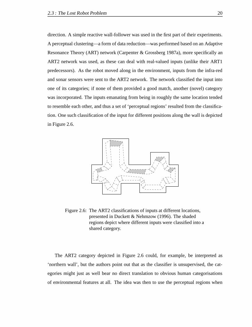
direction. A simple reactive wall-follower was used in the first part of their experiments.
A perceptual clustering—a form of data reduction—was performed based on an Adaptive
Resonance Theory (ART) network (Carpenter & Grossberg 1987a), more specifically an
ART2 network was used, as these can deal with real-valued inputs (unlike their ART1
predecessors). As the robot moved along in the environment, inputs from the infra-red
and sonar sensors were sent to the ART2 network. The network classified the input into
one of its categories; if none of them provided a good match, another (novel) category
was incorporated. The inputs emanating from being in roughly the same location tended
to resemble each other, and thus a set of ‘perceptual regions’ resulted from the classifica-
tion. One such classification of the input for different positions along the wall is depicted
in Figure 2.6.
Figure 2.6: The ART2 classifications of inputs at different locations,presented in Duckett & Nehmzow (1996). The shadedregions depict where different inputs were classified into ashared category.
The ART2 category depicted in Figure 2.6 could, for example, be interpreted as
‘northern wall’, but the authors point out that as the classifier is unsupervised, the cat-
egories might just as well bear no direct translation to obvious human categorisations
of environmental features at all. The idea was then to use the perceptual regions when

2.3 : The Lost Robot Problem 21
trying to localise. A list of hypotheses, originally consisting of all input-matching per-
ceptual regions, was formed if the robot ‘became lost’. Then the robot started to move
and could strengthen and weaken hypotheses each time it had moved a certain distance,
or depending on which other ART2 category would become active (the best match) next.
Detecting and weighing the hypotheses based on transitions between categories was thus
part of the approach. One of the strengths of this approach is that the experimenter does
not have to explicitly specify the number of landmarks (ART2 categories) that should be
extracted. New landmarks could quickly be incorporated at any time through the addition
of new prototypes. A problem with this approach, as the authors point out themselves
is, however, that noisy or ‘rogue’ input patterns will result in spurious ART2 categories,
i.e. categories which will never again match the inputs very closely. We thus would end
up with several regions in input space which will rarely—if ever—be visited again by the
sensory signal. Another problem was that of ‘over-training’, as prototypes were dragged
away through their constant updating. The holes formed in input space would then rapidly
be covered by the incorporation of additional categories by the ART2 network, causing
a re-classification of inputs which previously were classified as belonging to one of the
earlier types. A sort of abstraction of the sensory data stream, into perceptual regions,
was thus formed.
A later approach, based on the same ideas as in the ART2 system, was presented by
Owen & Nehmzow (1998b). The goal was again to form a set of landmark represen-
tations bottom-up from the sensory data and to use these for localisation. This time, a
simplified version of the Restricted Coulomb Energy (RCE) classifier5, was used to ex-
tract the landmark representations. Each landmark corresponded to a class of inputs, and
was represented using a prototype, called a representation vector, or an R-vector. A data
reduction was thus performed based on the R-vectors. As inputs arrived into the system,
they were compared to the existing R-vectors, using a similarity measure like the dot
product. If the input closely matched6 an R-vector in the system, the input was classified
5A description of the original RCE model can be found in Hudak (1992).6A fixed threshold was used for specifying what a ‘close enough’ match to existing R-vectors
constituted.

2.3 : The Lost Robot Problem 22
as belonging to that class, and nothing else happened. If, on the other hand, none of the
existing R-vectors matched the input, a new R-vector was placed at the new input loca-
tion, i.e. the system had just learnt a new landmark representation. That is, a constructive
(resource-allocating) approach was used for the incorporation of landmarks. Effectively,
this approach did the same work as the ART2 network, only in a much simpler manner.
Again, a data reduction was thus performed, this time based on the R-vectors.
sensor 2
sensor 1
R−vector (class prototype)
Figure 2.7: A 2-dimensional input space depiction of the sort of RCEclassifier used in Owen & Nehmzow (1998b).
The vector map of the environment was then built by moving the robot around the
environment, and keeping track of the matching R-vectors. When the sensory readings
changed enough to cause another R-vector to become the best matching, for at least 4
inches of movement7, this was added to the map, along with information about the com-
pass direction and distance between the landmarks. The same problem as with the ART2
approach remained, however, as pointed out in Nehmzow (2000). Namely, any single
non-matching input would create a new prototype. Situations where sensor activations
changed would thus lead to many intermediate prototypes, depending on how the indi-
vidual elements of the sensor vector changed, and because of noise. That is, the RCE
7It is unclear as to how many time-steps this corresponded to.

2.4 : Discussion 23
classifier dropped a dense trail of R-vectors (prototypes) as it tracked the path of the
sensory signal throughout input space. Thereby many regions never to be visited again
would be incorporated. The concepts were not used to control the robot in any manner;
no control loop was formed.
2.4 Discussion
The reviewed approaches for Route Learning involved the extraction of a less detailed
representation of the data, i.e. data reduction. The techniques were based on either a
manual set of reduction criteria (branch points), or some sort of more general unsuper-
vised extraction. This was done by using clustering algorithms like Self Organising Maps
or prediction learners like the Mixture of (Recurrent) Experts. Learning a route then
involved keeping track of the order in which the units or experts, respectively, were ac-
tivated. As the number of units or experts was lower than the sensory dimensions, this
meant that a sort ofspatial filteringor reduction had taken place. If the same unit or
expert became active for several time-steps in a row, this could also be used for atem-
poral filtering or reduction, i.e. a sort of dynamic time warping, as the repetitions could
be removed or run-length encoded. The same sort of unsupervised techniques were also
applied to the Novelty Detection problem. In the reviewed papers, a hierarchy of predic-
tion networks and a variant on the SOM were used instead of storing all individual inputs.
Finally, in the Lost Robot Problem, we again find unsupervised techniques, specifically
Adaptive Resonance Theory and Restricted Coulomb Energy clusterers.
The common approach to dealing with these problems, in all of the reviewed papers, is
thus to reduce the amount of data in some manner. A variety of unsupervised techniques
had been used to accomplish this. In the next chapter we look at what the differences are
between these techniques, as well as the similarities. We construct a general framework
which encompasses these, and try to make explicit the assumptions behind the way they
filter or reduce the data. Would these techniques work if we wanted to do learning on the
reduced data, as well?

Chapter 3
Data Reduction and Event Extraction
�HERE ARE SOME COMMON PROPERTIESwhich all the reviewed data reducers
in the previous chapter exhibit. Namely, they all maintain a set of regions or
trajectories according to which the inputs can be classified. At the end of this chapter, we
provide a general framework for constructing a data reducer which produces descriptions
that are also suitable for learning. The framework involves keeping a set ofexpertswhich
are—as the name succinctly suggests—specialised at different regions or trajectories in
sensory space. Transitions between these experts are detected by asignalling function,
which forms and outputs representations depicting the novel sensory situations. Different
alternatives for realising and training the experts are reviewed. Instead of using overall
compression error as a training criteria, we suggest that the area of change detection is
more in line with what we need because then input distinctness rather than density is
considered. We suggest that data reduction based on change detection principles could
be dubbed asevent extraction, as what will remain is just the time points corresponding
to significant transitions in sensory space. In the next chapter, a novel unsupervised data
reducer (event extractor) is then created based on the principles presented here.
24

3.1 : Data Reduction 25
3.1 Data Reduction
As discussed in the previous chapter, in order to cope with the tasks, the systems em-
ployed some sort of data reduction technique. This typically involved an unsupervised
mechanism, to allow the system to form and adapt its own representations, rather than
base it on some fixed pre-defined criteria.
3.1.1 Experts
If we inspect the employed unsupervised mechanisms (we include the prediction networks
here as well), they all maintain some set of input space regions or trajectories according
to which the incoming data is classified. As we are looking for general properties, we
suggest that the data reducer is considered as maintaining a set ofexperts, according to
the mixture scheme put forth by Jacobs et al. (1991). These expertscompetein accounting
for the inputs. This description applies to the systems reviewed in the previous chapter,
in the following manner.
One of the reviewed approaches (Tani & Nolfi 1998) for implementing said experts
is to use Recurrent Neural Network (RNN) modules; each module constitutes a separate
expert. The recurrent connections of the modules can maintain varying amounts of con-
text, thereby allowing each expert to cover trails in input space of different lengths. These
modules compete with each other by predicting the next input; the module producing the
best prediction (closest to the actual coming input) will become the winner in this compe-
tition. A similar approach would be to use Hidden Markov Models (HMMs) as experts.
Such an approach was put forth by Liehr & Pawelzik (1999), where a mixture of HMMs
was used for time-series segmentation. The training of such experts would, however, take
considerable time as special care is needed to avoid local minima (by for instance using a
simulated annealing approach).
A simpler approach is to use model vectors in a vector quantiser (VQ), like the
Self Organising Map, letting each model vector correspond to an expert, see (Owen &

3.1 : Data Reduction 26
Nehmzow 1996, Nolfi & Tani 1999). Using this method, there is a clear one-to-one map-
ping between inputs and VQ experts, as each input belongs to one—and only one—expert
through the Voronoi cell partitioning. Knowing the current VQ expert thus confines the
possible current input locations to a higher degree (to a certain Voronoi cell) than the
sequence-based approaches described above, which can have any number ofoverlapping
regions. Thereby the VQ would provide a means forinverting the experts back to the
input, i.e. knowing the expert at a particular point in time, we could find out approxi-
mately what the particular input should have been by looking at the model vector. (This
is the very idea behind VQ, namely that it can be used for some sort of compression and
subsequent decompression of a signal.) The extracted VQ experts thus lend themselves to
fairly transparent analysis. Further, finding out the similarity between VQ experts, primar-
ily for generalisation, can involve a straight-forward Minkowski (for instance Euclidian)
distance calculation between their respective model vectors. Calculating the similarity or
distance between a set of RNN modules is considerably more difficult as information is
encoded into weights and intertwined with the delay conditions. The RCE method used
by Owen & Nehmzow (1998b) has R-vectors which also resemble the VQ model vectors.
Similarly, as we discuss in Section 4.2.3, the working of the ART networks used in for
instance Duckett & Nehmzow (1996) can also be implemented to a fairly accurate degree
using VQ model vectors. Vector quantisation is thus a quite common and straight-forward
approach for dealing with the data reduction, and the one we will focus on in this thesis.
We now take a more detailed look at what vector quantisation is and how it can be used.
3.1.2 Vector Quantisation
Vector quantisation (VQ) is commonly used for data compression and analog-to-digital
conversion; for an overview see Gray & Neuhoff (1998). At the heart of the VQ is a
set of model vectors, or prototypes, also called thecodebookof the VQ. In the simplest
form, these model vectors are of the same dimensionality as the inputs, representing dif-
ferent clusters of input patterns by a prototypical pattern roughly in the centre of each

3.1 : Data Reduction 27
cluster. A distance function assigns individual inputs to one of the model vectors, work-
ing like a nearest neighbour classifier. Instead of storing or transmitting the individual
high-dimensional inputs, the low-dimensional index of each winning model vector can
be stored or transmitted. The original input can then be reconstructed—with some loss
of information—by inverting this process, looking up and producing the particular model
vector (input pattern) which the index corresponds to in the codebook. Traditionally, VQ
performance is defined (Fowler & Ahalt 1997, Buhmann & Hofmann 1997) usingrate
anddistortion:
� Rate corresponds to the size needed to represent the winning model vector. There
is a clear relationship between the rate and the size of the codebook, especially if a
fixed-rate VQ is used, as explained by Hwang, Ye & Liao (1999). Generally, a low
rate can only be achieved if very few model vectors are used, and a higher rate is
required for representing a greater number of model vectors.
� Distortion corresponds to the information loss which is incurred as inputs are mapped
to the model vectors. A low distortion means that the model vectors accurately
match the input, while a high distortion implies a large loss in signal quality.
Clearly, the more model vectors that are used in the VQ (the higher the rate), the
more readily can inputs be mapped to a close-laying model vector (lower distortion). An
arbitrarily low distortion can thus be achieved by controlling the rate; in the extreme an
individual model vector can be used for each input, in which case there is no distortion at
all, but at the cost of having averyhigh rate. In the other extreme, a single model vector
could be used for the entire input set, i.e. a very low rate, thereby however inevitably
causing a very high distortion as all the different inputs are mapped to this single model
vector. There is thus atradeoff between rate and distortion. Depending on the domain,
this tradeoff is quantified using either an operational distortion-rate function or a rate-
distortion function. That is, either the distortion is measured if a certain fixed rate is used
(distortion-rate) or the rate is measured which gives a certain allowed distortion (rate-
distortion). Different configurations (placements) of model vectors on a given dataset

3.1 : Data Reduction 28
can thus be compared using rate and distortion. Ideally, the placement leads to both low
distortion (no quality loss) and low rate (compact compressed size). As long as the VQ
is used only forcompression, this focus on rate and distortion is entirely appropriate. We
however argue that iflearning, based on the extracted model vectors, is to be performed,
this is no longer appropriate. In the following we look at the underlying assumptions of
compression, and the way that compression quality is measured.
3.1.3 Compression
There exists a number of existing methods forcompressingtime-series data. These meth-
ods can be divided into two broad categories, namelylosslessandlossycompression. The
difference between these types of compression is in the tolerance forcompression error,
i.e. the degree that a compressed and then decompressed signal differs from the original
signal. Lossless compression implies, as its name suggests, a compression which entails
absolutely no degradation of the quality of the signal, were it to be decompressed. The
compression error of such a method is thus always zero. These types of compression algo-
rithms are readily employed when no degradation of the data can be accepted, like when
compressing text documents. Lossy compression instead accepts a limited degradation
of the signal as part of the compression, thereby most often leading to a greater (better)
compression ratio(original uncompressed size / compressed size). The lost information
is usually removed because it is considered less important to the quality of the data (usu-
ally an image or sound) or because it can be recovered reasonably by interpolation from
the remaining data.
In mobile robotics, lossy compression is in most cases acceptable, or perhaps the
only viable option as it is the only ready means for achieving an acceptable compression
rate. As most data originates from noisy, and essentially analogue sampling processes, it
does not constitute a perfect account in the first place. Lossy compression techniques are
commonly based on re-coding the data using wavelets, vector quantisation, or recently
even using fractals (iterated function systems).
The performance of a lossy compressor is normally defined as the compression rate,

3.1 : Data Reduction 29
given a certain allowed compression error, or alternatively, the compression error for a
certain given compression rate. That is, the technique which produces the lowest overall
error when decompressing data of a certain compressed size (say 100 KB) is considered
the better one. (Note the correspondence to the way performance of a VQ is defined.)
There are of course exceptions from this performance criterion, for instance involving the
subjective evaluation of decompressed image or waveform quality. Such an evaluation
is, however, only applicable for very specific domains, and implicitly assumes that some
set of particular characteristicsalwaysis the relevant one, regardless of the particular ap-
plication (for instance faithfully capturing the edges of surfaces, or to ignore differences
in very dark colours). The commonly used, domain independent, performance criterion
is thus to calculate some sort of overall error, like the squared error between the original
and the decompressed signal1. Through this performance criterion, different compres-
sion mechanisms can be compared with each other. Note that constructing a good lossy
compressor, for example based on vector quantisation, is thus analogous to doingerror
minimisation. We now look at how error minimisation is accomplished.
3.1.4 Error Minimisation
Techniques based on error minimisation all have some sort ofcost function, which is to
be minimised. Doing compression, this cost function usually is adistortion measurethat
quantifies the cost resulting compressing input�, and then decompressing this to��. The
bit rate of the encoding can also be taken into account, often in a Lagrange approach
where the importance of distortion compared to bit rate can be specified, see e.g., Gray &
Neuhoff (1998) for details. The most common distortion measure is based on the squared
error���� ��� � ��� ����. When a sequence of data��� � � � � �� is compressed, an average
(overall) distortion error� can be defined:
� ��
�����
����� ���� (3.1)
1For a comprehensive review of this the reader is referred to Gray & Olshen (1997).

3.1 : Data Reduction 30
If the distortion measure is based on the squared error,� would correspond to the mean
squared error. A good lossy compressor would have an� close to zero; minimising�
is thus the goal for almost all existing compressors, or techniques which can be used for
compression.
Note that there may be � instances of the same input� which is to be compressed.
If the compressor ‘learns’ to compress and decompress this input better, the payoff is thus
-fold, compared to learning another input with an equal distortion but which occurs
only once. An effective compressor thus takesinput densitiesinto account, focusing its
resources on the most frequent inputs, as pointed out in Gray & Olshen (1997). Infrequent
inputs can be admitted a higher individual distortion as they do not affect� to a significant
degree by themselves.
Thisdensity approximationor density estimationoften takes place by repeatedly mak-
ing small adjustment to the parameters, the magnitude of which gradually are reduced as
the system is ‘cooled down’ to a final resting state, in an annealing process. The idea is
that this final state has managed to adequately capture the underlying input densities as
the frequent inputs will have influenced the parameters to the greatest degree. This is,
however, also a reason why the learning process often is slow in error minimising sys-
tems. The annealing process must namely not proceed in too large jumps, i.e. too large
reductions of the temperature, as pointed out by Rose (1998), or it may miss the good
solutions. Further, this density approximation could be completely overturned if the in-
ternal resources were extended or modified during the process. Therefore, a fixed number
of resources, e.g., model vectors in the case of a vector quantiser, is commonly employed
during the entire process, or the density approximation might have to be restarted or re-
computed to some extent.
3.1.5 Error Minimisation for Experts
Is error minimisation really appropriate for training our experts? We argue that it is not,
and that there is a fundamental problem with using data reducers based on error minimi-
sation in the mobile robotics domain, especially if you want to do learning. Consider

3.1 : Data Reduction 31
Nolfi and Tani’s data reducer (Nolfi & Tani 1999), described in Section 2.2. They let a
vector quantiser represent the different experts using its model vectors, each model vec-
tor corresponding to a separate expert. They reported difficulties with working directly
with the inputs as infrequent (underrepresented) inputs were not picked up by the model
vectors at all. They instead introduced a prediction network with a set of internal nodes,
and let the vector quantiser work on these internal nodes. The system could now handle
infrequent inputs to a somewhat better degree, as differences had been enhanced a little
in this process.
The reason for these problems becomes clear when we consider how the vector quan-
tiser was trained; it tried to minimise the overall (mean squared) error between the inputs
and its model vectors. Most of the time their wall-following robot received virtually the
same input, namely a wall on the right-hand side and nothing on the front, left, and back
sensors. Quite distinct but infrequent inputs arriving when passing doorways or corridors
(activation on left sensors as well), entering corners (activation in front) and leaving them
(activation in back) were ignored. That is, none of the model vectors came to represent
these inputs, as they did not constitute a significant part of the overall error. By map-
ping inputs to a hidden layer, the quantitative differences between the common inputs
and the infrequent ones were emphasised somewhat. This forced the vector quantiser to
take them somewhat more into account as they now caused a greater individual distortion,
their hidden activation patterns beingverydifferent from the common inputs’.
An unsupervised data reducer which bases its experts on input densities, performing
error minimisation, is thus subject to difficulties. In the extreme, the system will become
expert at recognising slightly differing wall inputs, whilecompletely ignoringdoorways,
corners, junctions, etc., all being absolutely essential for a robot performing even the
simplest of localisation tasks.
If the input distribution is completely stationary, the error function can certainly be
modified as to balance orweighinfrequent input areas higher than infrequent ones. Thereby
small clusters can be given a greater effect, by for instance weighing dimensions where
there is a clear difference higher than other ones; the error minimisation approach would

3.1 : Data Reduction 32
then again be appropriate. However, this requires that the future distribution isknown
beforehand, otherwise this weighing is disruptive if new inputs arrive with distinct differ-
ences on these particular dimensions, thereby taking over the error term completely. The
data reduction should ideally not be based on any particular input distribution, but rather
be independent of the distribution, thus allowing the system to function under completely
different sensor configurations and in very different environments.
The frequency (density) of the different inputs thus comes to play too great a role
in error minimisation. There are, however, alternatives to basing the experts on error
minimisation, namely from the area ofchange detection. Let us take a closer look at
change detection and how it applies to our needs.
3.1.6 Change Detection
Change detection involves the prompt and reliable detection of changes in signal char-
acteristics, like a change in signal mean or variance. For an overview of this area, the
reader is referred to Basseville & Nikiforov (1993). Generally, the focus is on detect-
ing when changes occur from matching a current situation��, to some other situation��.
Change detection could be used iteratively (��� ��� ��� � � � ) to segment a sequence into dif-
ferent parts. The change detector thus detects and signalsthat something has happened,
at different points in time.
However, an additional processing system would be required that determinedwhathas
happened, in order to avoid having to treat each situation as completely novel. Thereby
re-occurrences of previously encountered situations can be detected, e.g., that��� actually
corresponds to the earlier situation��. This entails that all encountered situations should
be stored for future reference, in some manner. This is where our experts come in. If
a vector quantiser could be used for the change detection, the different situations could
correspond to the model vectors in the system (for instance the different signal means
that are encountered). The difference between how prototypes are placed in a vector
quantiser based on error minimisation versus change detection is illustrated in Figure 3.1.
Error minimisation treats the signal peak as an outlier—thereby ignoring it—and instead

3.1 : Data Reduction 33
focuses on the two quite similar but frequent types of input. Change detection, on the
other hand, focuses on only the points in time where changes occur, effectively ignoring
the intermediate stages. Change detection would thereby be much more appropriate for
determining experts.
Error minimisation
a b a b a
a
b
x(t)
prototype
prototype
t
Change detection
a
a
b
x(t)
prototype
prototype
ba
t
Figure 3.1: Error minimisation (top) places prototypes according toinput frequency while change detection (bottom) insteadfocuses on distinctness.
One simple technique for change detection is the Finite Moving Average (FMA) al-
gorithm, which encodes the current situation using a bounded interval of past inputs, see
Basseville & Nikiforov (1993). This concept has been the basis for the unsupervised data
reducer presented in the next chapter. It utilises a finite moving average to represent the
situation which the robot currently is in and at the same time filters the noisy input signal
to some extent. Rather than referring to this approach as ‘data reduction based on change
detection principles’, we suggest that ‘event extraction’ would be quite appropriate. There
already exist some techniques for this, which we will take a look at in the following.

3.2 : Event Extraction 34
3.2 Event Extraction
Generally, event extraction involves the discretisation of a continuous-valued stream of
sensory readings into a stream of intermittent events. We look at an existing approach
for event extraction and discuss the concept of an ‘event’, like what type of information
they are supposed to convey, whether all events need to be relevant, and where they are
supposed to come from. We propose the interpretation that an event is a notification of a
transition between regions or trajectories in the sensory space, and if relevant leading to a
state change.
3.2.1 Related Work
The approach for event extraction, presented by Rosenstein & Cohen (1999), was also
based on maintaining a set of experts. These experts corresponded to stored prototypical
input subsequences, and a continual matching was performed against these each time-step
to find a winner. Their task was to classify different interactions with balls, cups, desks,
etc. Raw sensor readings were first transformed into clusters of time series that had a
‘predictive value’ to the agent. The approach was then based on keeping a set of proto-
types (experts), one for each category, namely the average of the cluster. Sequences were
incorporated into the clustering based on a pre-defined set of simple rules, ortemplates,
depicted in Figure 3.2. Each template corresponded to a sharp rise or drop of a sensor.
When one of the templates matched the input, i.e. a change was detected in one of the
sensors, aneventwas generated. All other sensors which also exhibited such a sudden
change within a 800 ms window, were considered to be part of the same event. When
an event was triggered, the actual sensor values were recorded for a five-second window
for each of the sensors. Each sensor’s five-second sequence was then sent to a clustering
algorithm. Recurring situations would thus be extracted as clusters of similar five-second
sequences. A prototype (average sensory sequence) was extracted for each cluster. The
number of clusters was pre-defined by the experimenter; the same number was used for
each and every sensor. Each such cluster of inputs, represented by a prototype, could
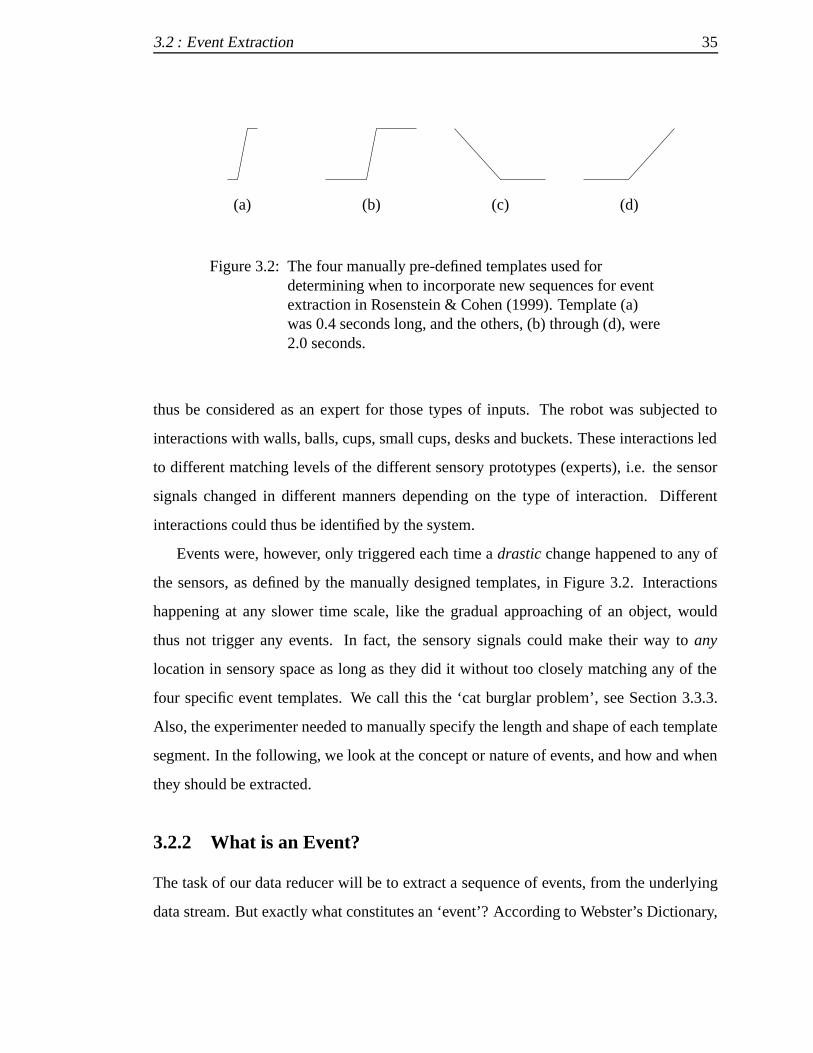
3.2 : Event Extraction 35
(a) (b) (c) (d)
Figure 3.2: The four manually pre-defined templates used fordetermining when to incorporate new sequences for eventextraction in Rosenstein & Cohen (1999). Template (a)was 0.4 seconds long, and the others, (b) through (d), were2.0 seconds.
thus be considered as an expert for those types of inputs. The robot was subjected to
interactions with walls, balls, cups, small cups, desks and buckets. These interactions led
to different matching levels of the different sensory prototypes (experts), i.e. the sensor
signals changed in different manners depending on the type of interaction. Different
interactions could thus be identified by the system.
Events were, however, only triggered each time adrasticchange happened to any of
the sensors, as defined by the manually designed templates, in Figure 3.2. Interactions
happening at any slower time scale, like the gradual approaching of an object, would
thus not trigger any events. In fact, the sensory signals could make their way toany
location in sensory space as long as they did it without too closely matching any of the
four specific event templates. We call this the ‘cat burglar problem’, see Section 3.3.3.
Also, the experimenter needed to manually specify the length and shape of each template
segment. In the following, we look at the concept or nature of events, and how and when
they should be extracted.
3.2.2 What is an Event?
The task of our data reducer will be to extract a sequence of events, from the underlying
data stream. But exactly what constitutes an ‘event’? According to Webster’s Dictionary,

3.2 : Event Extraction 36
an event is:
a noteworthy occurrence or happening : something worthy of remark : an
unusual or significant development
This definition suggests that events are significant, or noteworthy, i.e. that they carry
some sort of informational value. This begs the question whether there can be any in-
significant events, i.e. whether unimportant orirrelevant occurrences could generate
events. We will get back to the idea of relevance and irrelevance shortly, but let us first
take a look at the area of Discrete Event Systems, which is based around the very idea of
events. Events are the basic units in the area of Discrete Event Systems (DES), which—as
we will see—is what we want the system to effectively self-organise into. Introductions to
DES theory can be found in Cassandras (1993), Banks, Carson & Nelson (1996) and Fish-
man (2001). In DES, the events, or more specifically their triggers, are usually defined by
the experimenter. The goal of the DES modeller is then to find an appropriate description
of the underlying event-triggering system, e.g., for descriptive purposes. Another aim is
to let the system react to the events, in order to keep it stable under varying conditions,
i.e. for system control. Thanks to the discretisation of any continuous-valued input stream
into an event stream, according to pre-defined triggers, useful temporal relationships can
be found using virtually any standard learning technique. A common abstraction in the
DES area is to view the system as a Finite State Automaton (FSA) or a Petri Net model.
In the FSA case, there is a discrete number of states which the system jumps in-between,
when events occur. The definition of an ‘event’ is therefore tinted by this perspective. Let
us look at three definitions of ‘events’ from different introductory texts to DES theory.
The first definition is a very succinct one:
A change in state of a system. (Fishman 2001, page 39)
In this definition, events simply are described as state changes. A slightly more de-
tailed definition is:
An instantaneous occurrence that changes the state of a system (such as
an arrival of a new customer). (Banks et al. 1996, page 60)

3.2 : Event Extraction 37
Here, they point out that the changes should be considered as instantaneous. Again,
the definition also talks aboutchanges, but now point out that they are the result of the
event, i.e.causedby the event. Finally, some DES texts do not even try to formally define
the concept, as the risk of being overly specific may inadvertently exclude too much from
the event concept, or include undesired phenomena:
As with the term “system”, we will not attempt to formally define what an
“event” is. It is a primitive concept with a good intuitive basis. We only wish
to emphasise that an event should be thought of as occurring instantaneously
and causing transitions from one discrete state value to another. (Cassandras
1993, page 36–37)
These definitions all relate events tochange, specifically to a change of the system
state. States are explicitly represented (as circles) in state transition diagrams, like in
Figure 3.3. Reacting to an event in DES thus simply corresponds to following an arc
in the state transition diagram. It is worth noting that there are many cases in which an
event does strictly speakingnot lead to a state change, namely in cases where there are
recurrent connections (self-transitions) to a state. For example, in Figure 3.3, if the system
is in state ‘1’ and the event� arrives, the result will be to stay in the same ‘1’ state, i.e.
there in fact isnosystem state change. There is, however, atransition, but the definitions
of events explicitly discuss state changes and not transitions.
b
a
ab
Start0 1
Figure 3.3: A simple two-state FSA which only accepts (shaded state)event sequences ending with an�. Events here correspondto simple transitions.
3.2 : Event Extraction 38
Do state changes have anything to do withrelevance? Consider events which in each
and every state lead to a self-transition. Such an event could be considered as irrelevant,
as it does not produce a state change, and it would always be the same whether or not the
event had occurred. This also gives us a notion of relevance: being relevant corresponds
to being worth reacting to or keeping track of. Accepting this line of thought,irrelevant
eventscan thus occur in DES systems; an oxymoron considering the Webster’s dictionary
definition of ‘event’ in the beginning of this section.
A straight-forward interpretation of ‘relevance’ is to relate it to some sort of task
performance. That is, is the event relevant for task performance? This typically would re-
quire some sort of performance feedback (reinforcement) signal. Making things difficult,
in an on-line learning system, relevance may change, in that the performance evaluation
function may be altered during operation2. Things (events) which do not currently need
to be reacted to, i.e. incur no state change, can become relevant at some later stage, and
then need a state change. An informal description of our view of events would be:
DESCRIPTION An EVENT is a notification of an occurrence in sensory space which
could result in a state change.
This description certainly leaves many questions unanswered, like what is a ‘notifica-
tion’, what do these notifications look like, and what exactly constitutes an ‘occurrence’?
The nature of events relates to the manner in which they are triggered, i.e. the sorts of
occurrences in sensory space that we are to be notified about. The question becomes one
of how and when events are to be triggered, or simply ‘where do events come from?’.
3.2.3 Where do Events Come From?
In DES theory, the events emanate from well-defined discrete sources like a user pressing
a key on a keyboard, a customer entering a queue, or a product arriving into a warehouse.
2It is therefore generally also good to follow an exploration strategy in which the system never convergesonto a single fixed behaviour, but which instead always keeps testing alternative solutions at some low baserate. We construct such a system (Learner II) in Chapter 7.

3.2 : Event Extraction 39
Some of these events can be uncontrollable, i.e. the occurrences of these cannot be af-
fected. There also usually is a set of controllable events, the occurrence of which can
be affected by the system’s actions, thereby allowing for (supervised) control. The actual
detection and triggering of the events from continuous and noisy sources is thus, however,
not a central part of DES theory; it simply regards the events as inputs arriving from some
sort of existing, pre-defined, event detector or extractor3.
The event extractor receives as input a continuous-valued, typically high-dimensional,
data stream, and is to produce a stream of discrete events as outputs. These events
should capture the relevant information in signal space. Exactly what isrelevantis highly
task-dependent, and the approach we take in the following is to first just extract a goal-
unrelated event stream—a sort of general abstraction of the data stream—and then as a
successive stage filter away the events with low informational value. An alternative would
be to only extract the events which are directly relevant for performing the task, but this
would prove difficult, as we generally do not know beforehand what the relevant inputs
are for such selective event triggering and it is difficult to learn this at the time-step level.
This relates to the chicken-and-egg problem we discussed in the introduction: how can we
extract only relevant events when we cannot assign relevance unless we have performed
the extraction? Extracting a quite general stream of events denoting the major changes,
and then assigning credit to these events, is our approach for dealing with the problem.
As mentioned, events are notifications of occurrences in the sensory space which of-
ten should lead to state changes. It is not enough to be notified justthat something has
happened in sensory space, we also want to knowwhat has happened. That is, just re-
ceiving a message saying ‘an event has occurred’ is not very useful. Instead, a message
saying ‘an event� has occurred’ or ‘an event� has occurred’ gives us the basis to react in
a context dependent manner. The event extractor thus should be able to output messages
for us, containing different events, relating to different sensory conditions. Existing ap-
proaches for this, or rather for data reduction, reviewed in the previous chapter, are based
3The distinction we make between an event detector and an event extractor is that the detector justdetects and signals event instances from a set of event triggers, whereas the extractor forms the set oftriggers on its own, either through an unsupervised or a supervised learning process.

3.2 : Event Extraction 40
on a partitioning of the continuous input space into a set of regions. Movementsbetween
these regions then trigger events, whereas movements of the sensory signals within one
and the same region do not cause any output from the event extractor. Each region could
thus be thought of as representing a single global state of the sensors; only when this state
changes drastically enough to enter another region, is a notification sent in the form of an
event. The event typically indicates the now best-matching region. The problem is thus
cast as a classification problem, where the system forms a set of clusters (class regions)
from the input data and uses transitions between these clusters as event triggers.
It is worth noting that the granularity of this partitioning indirectly determines the rate
at which events are fired. In one extreme, where the entire input space is considered as
one single region, there will never be any transitions to signal. In the other extreme, a
single (tiny) region is created for each and every input which can be received. Then at
each time-step, an event will be triggered4, and we will be back at something like the
time-stepped input we started with in the first place. Generally, the more regions we
split the input space into, the greater the likelihood for triggering an event. Finding an
appropriate granularity for event extraction is a difficult problem, which we, however, get
back to in later chapters. Part of the solution we propose is that the number of regions
be determined somehow based on the complexity or distribution of the inputs, rather on
somead hocfixed value, conjured up by the experimenter.
3.2.4 Discussion
So, what is an event? As discussed in Section 3.2.2, we view an event as a notification
of an occurrence in sensory space. The event may result in a state change, if it is worth
keeping track of, i.e. if it isrelevant. This is by definition task-specific and we get
back to this in later chapters where we look at learning based on the extracted events.
The ‘occurrences’ in sensory space correspond to one of two things, in as far as existing
approaches are concerned, at least. Either they correspond to moving to another region
4Unless the exact same input arrives repeatedly; however, highly unlikely if the inputs are based onnoisy analogue sensors.
3.3 : A General Event Extraction Framework 41
in input space—a straight-forward classifier or clusterer could determine this—or they
correspond to a switch in trajectory through the input space. The latter would require that
different, possibly overlapping, sequences would be kept track of, e.g., through a set of
RNN modules or possibly some form of explicit input sequence prototypes. While RNN-
based techniques were used by Tani & Nolfi (1998) and Nolfi & Tani (1999), whether they
actually represented any overlapping input space trajectories or just performed a more-or-
less standard partitioning is very much in question. (As is shown in coming chapters, the
exact same segmentation of the sensory stream is namely achieved using a simple vector
quantiser.) An important thing to also note is that none of the existing data reducing
(possibly event extracting) approaches actually involve the robot reacting to the events.
That is, none use the events for mobile robot control. This would require that a number
of issues be dealt with, relating to getting a continuous motor output signal from a more
or less static (discrete) event based specification. We deal with all these issues in later
chapters.
3.3 A General Event Extraction Framework
We now try to summarise the properties which are common for the existing data reducers
or ‘event extractors’. In order to perform an effective data reduction, the system needs
to be able to detect repeated occurrences, or recurrences, of situations. This is done by
maintaining a set of experts. When the inputs change enough to no longer match the
current situation (expert), an event is generated.
3.3.1 Definitions
We consider it prudent to view the extractor as working on three distinct spaces. First,
there is an input space where the inputs arrive each time-step. This space can be quite
different from the second (internal) state of the extractor—the so called extraction space—
which is also updated each time-step. The extraction space is used for detecting events
caused by changes in input space. The third space is the event space, where outputs are

3.3 : A General Event Extraction Framework 42
produced from the extractor at intermittent points in time, in the form of events. The event
extraction involves both a spatial and temporal filtering of the input stream, as discussed
in the following.
DEFINITION The fixed-sizeINPUT SPACEprovides signals to the control system from
the hardwired (fixed) sensory array of exteroceptive and proprioceptive
sensors.
In order to avoid having to treat each change in input characteristics as something
completely novel—a similar situation may have been encountered previously—the event
extractor needs to store or maintain the characteristics of the encountered situations. This
can be done in a variety of ways, as shown above; the underlying idea is that the event
extractor maintains a set ofexperts.
DEFINITION An EXTRACTOR EXPERT or just EXPERT constitutes an input-
accounting sub-system of the extractor. Typically, a limited number of
experts are maintained by the extractor, each specialising in a particular
sub-set or sub-sequence of inputs.
The experts should be considered as providing only a local (current, or short-term)
account of the state of the system, as they do not contain information about the global
history of the system. This provides a sort ofspatial filteringas individual inputs are
transformed to a—usually lower-dimensional—extraction space.
DEFINITION The EXTRACTION SPACEcontains the internal time-step based repre-
sentation of the event extractor, depicting how the experts match the
current input. This space is not necessarily fixed-size, depending on if
a static or dynamic number of experts is used.
As long as the incoming inputs are accounted for accurately by the current expert, no
event is to be signalled.

3.3 : A General Event Extraction Framework 43
DEFINITION A SIGNALLING FUNCTION tracks changes in extraction space and sig-
nals an event at the current time-step� if the location in extraction space
at time-step�� � was ‘different enough’.
If the representations in extraction space are orthogonal, like the winner-take-all result
of an input classification, detecting such a change is trivial. Otherwise, a criterion for
being ‘different enough’ in extraction space to warrant a event signalling needs to be
defined, generally allowing minor changes of input characteristics to occur without taking
action.
DEFINITION An EVENT is a change in extraction space as notified by the signalling
function.
The focus on reporting only the changes leads to a sort oftemporal filtering, as redun-
dant inputs are removed from the stream. For clarity, it is worth noting that several events
are never signalled at the same time-step, nor in-between time-steps, as such changes
would all be compound into one through the sampling process occurring at each time-
step.
DEFINITION The EVENT SPACEcontains the output representation from the extrac-
tor. The representation is based on either the extraction space, the input
space, or a combination thereof. This space may change size dynami-
cally, depending on the chosen event representation scheme.
In the simplest case, there is a one-to-one correspondence between experts and points
in the event space. That is, every situation where a certain expert is best at accounting
for the current input, a particular output is produced by the extractor. If a new expert is
incorporated dynamically (on-line) by the system, this will then affect the event space
accordingly.

3.3 : A General Event Extraction Framework 44
3.3.2 Example
An illustration of a simple event extractor is depicted in Figure 3.4. Here, each of four
experts corresponds to an input class or cluster, defined using a prototype input pattern.
In each time-step, the input is classified as belonging to one of the experts. The extraction
space has four dimensions with a ‘1’ marking the best matching expert, and zeroes for
the others. Changes in extraction space are signalled as events by the signaller, and the
output corresponds directly to the expert representation, i.e. events are represented using
a bit string of length four with only a single bit active (a localistic event representation).
[0.8 1.0 0.5 0.5 0.9 0.0]
[0.0 1.0 0.5 0.5 0.9 0.0]
[0.1
1.0
0.5
0.5
1.0
0.0]
[0.0 0.0 0.5 0.5 0.0 0.0]
[0.0 1.0 0.5 0.5 1.0 0.0]
[0.7 1.0 0.5 0.5 1.0 0.0]
[0.1 1.0 0.5 0.5 1.0 0.0]
[0.0
1.0
0.5
0.5
0.9
0.0]
[0.1
1.0
0.5
0.5
1.0
0.0]
[1.0 0.9 0.5 0.5 1.0 0.0]
[0.1
0.9
0.5
0.5
1.0
0.0]
[0.1 1.0 0.5 0.5 0.9 0.1]
[0.0
0.9
0.4
0.6
0.9
0.0]
[0.0
1.0
0.5
0.5
0.9
0.0]
[0.0 0.9 0.5 0.5 1.0 0.1]
[0.0 1.0 0.5 0.5 0.9 0.1]
[0.0 0.9 0.5 0.5 1.0 0.0]
[0.0
1.0
0.5
0.5
1.0
0.1]
[0.0
0.9
0.5
0.5
0.9
0.1]
[0.0
0.9
0.5
0.5
1.0
0.1]
[0.0 0.9 0.5 0.5 0.9 0.0]
[0.1 0.9 0.5 0.5 1.0 0.0]
Robot
[0.1 1.0 0.5 0.5 1.0 0.1]
[0.1 0.8 0.3 0.7 0.2 0.0]
[0.0 0.8 0
.2 0.7 0
.5 0.1]
[0.0
0.8
0.3
0.7
0.7
0.0
]
[0.0
0.7
0.2
0.7
0.6
0.1
]
[0.1 0.8 0.3 0.7 0.1 0.0]
[0.0
0.8
0.4
0.6
0.9
0.0
]
[1 0 0 0]
[1 0 0 0]
[1 0 0 0]
[0 0 1 0]
[1 0
0 0
]
[1 0 0 0]
[1 0 0 0]
[1 0 0 0]
[0 1 0 0]
[0 1 0 0]
[0 1 0 0]
[1 0
0 0
]
[1 0 0 0]
[1 0 0 0]
[1 0 0 0]
[1 0
0 0
]
[1 0
0 0
]
[1 0
0 0
]
[1 0
0 0
]
[1 0
0 0
]
[1 0
0 0
][0
0 0
1]
Robot
[0 0
0 1]
[0 0
0 1
][0
0 0
1]
[0 0 0 1]
[0 0 0 1]
[1 0 0 0]
[0 0 0 1]
[1 0
0 0
]
[0 0 1 0]
[1 0 0 0]
[0 1 0 0]
[1 0 0 0]
Robot
[0 0 0 1]
(a) (b) (c)
Figure 3.4: (a) The multidimensional sensory input arriving at eachtime-step. (b) The unsupervised event extractor assignseach input to one of its experts, i.e. a spatial filtering. (c)Repetitions of expert assignments are removed and onlythe transitions remain, as events, i.e. a temporal filteringtakes place.
That is, in this simple setup:
� The input space is six-dimensional and real-valued.
� There are a total of four used experts in the example, each trying to account for the
signal in input space.

3.3 : A General Event Extraction Framework 45
� The extraction space is four-dimensional and binary.
� The signalling function detects and signals an event when the point in four-dimensional
extraction space moves.
� The event space is a four-dimensional copy of the extraction space.
Through this spatio-temporal filtering, redundant inputs are removed. Thereby mas-
sive amounts of history can be stored as the actual input or inputs need no longer be
stored themselves; instead the compressed (filtered) version thereof can be used. Ideally,
the global state of the system can be determined based on the sequence of extracted events
from the beginning of the system’s operation, i.e. by taking all available history (context
information) into account. In our description of an event extractor, the idea of maintaining
a set of extractor experts was included. These may in fact not be completely necessary, but
not having them will lead to limitations in the aforementioned spatio-temporal filtering,
as discussed in the following.
3.3.3 Doing Without Extractor Experts
Consider the special case where the extractor space is set to be identical to the input space,
i.e. no experts or any type of signal re-mapping is included in the extraction process. In
that case the extractor’s signaller works directly on the input, alerting when the signal is
‘different enough’ from one time-step to the next to warrant an event. That is, it monitors
changes directly in input space and only as long as the input is approximately the same
at time step� compared to� � �, i.e. below some threshold� (delta), it stays idle.
This is a very simple event extraction scheme, which works in some situations, but it has
problems. The�-based method may generate an inappropriate amount of events if the
signal-to-noise ratio is incorrectly reflected in the choice of�. If the threshold is set too
high, the extractor will miss the relevant changes, and a too low� setting will lead to
events being triggered by perfectly normal fluctuations. The problem corresponds to that
of acat burglar in a room with a motion sensor. In order to avoid false alarms from noisy

3.3 : A General Event Extraction Framework 46
sensor readings, the motion sensor has been equipped with a detection threshold; only
movements exceeding the threshold are treated as actual movements, the others as noise.
By doing a series of small movements, each one staying below the detection threshold,
the cat burglar is able to move to any location in the room without ever being detected!
This corresponds to a situation in which the inputs gradually have changed into something
drastically different without detection; obviously not an appropriate behaviour of an event
extractor. This problem remains as long as movements smaller than� can occur during
a single time-step. More importantly, while a�-method might detectthat something
has happened to the signal, it does not tell uswhathas happened. That is, each event is
treated as something completely novel and consequently any re-occurrences of previous
situations are not recognised as such. Thereby the input signal is just filtered temporally,
but not spatially as this requires that a limited number of recurring points are maintained
somehow in the system. As discussed, this can be done through a variety of techniques,
here summarised as being extractor experts.
An event extraction approach which was actually not based on having a number of
experts, but rather a predefined number ofevents(segment boundaries) was tested in
Himberg, Korpiaho, Mannila, Tikanm¨aki & Toivonen (2001). There, an off-line event
segmentation was performed on data collected from a mobile phone equipped with a
number of touch, light and interaction sensors. The sensory data was split into a pre-
defined number of segments based on ‘internal homogeneity’, i.e. segments with as low
variance as possible. The idea of having a set of experts that were competing for the
data was thus not considered. The problem with said approach is that this does not lead
to an effective data reduction, as each occurrence is treated as completely novel, and
generalisation (drawing on old or previous experiences) would thus not be possible. Each
segment could possibly be interpreted as a specific expert, but such a process would result
in subsets of virtually identical experts, due to re-occurrences of some situations. The
specified number of segment boundaries could thus instead be considered as an upper
bound on the number of resulting experts, the numbers being identical if each segment-
corresponding situation only occurs once in the data set.

3.4 : Discussion 47
3.4 Discussion
The focus of the previously used data reduction techniques, presented in the preceeding
chapter, was on minimising an overall compression error. That is, the reduction was
considered as an error minimisation problem where the entire dataset was to be captured
as accurately as possible. Infrequent inputs would, however, suffer the risk of being
ignored in this process. As discussed, it pays off for an error minimiser to perform a
density approximation, which however often takes quite some time to perform; often this
involves extensive subjection to the dataset. This also assumes that the distribution is
stationary, which needs not be the case in mobile robotics, where a robot may suddenly
enter a different environment where most inputs no longer match any of the previously
encountered ones. The density approximation becomes more difficult if the number of
experts is not kept constant throughout this process as previously assigned inputs may
have to be reassigned to the new configuration.
Ignoring infrequent but distinct inputs would be catastrophic in the area of mobile
robotics as these infrequent inputs may correspond to the few points where the robot
passes through doorways, junctions, etc., all of which are absolutely essential for suc-
cessful navigation and learning. We propose that the principles of change detection are
more in line with what we need, i.e. for event extraction. This should allow us to perform
an on-line and density independent extraction of experts from a continuous time series. In
the end of this chapter, a general event extraction framework was created, encompassing
the existing (compression based) data reducers. In the next chapter, we construct a novel
(change detecting) event extractor, based on this framework.

Chapter 4
The Adaptive Resource-Allocating
Vector Quantiser
�HE TRADITIONAL FOCUS on error minimisation, i.e. compression, is not appro-
priate for event extraction, as discussed in the previous chapter. Here, an alter-
native implementation is presented which instead is based on change detection. We start
out by formulating five basic principles of how the system should work, and relate these
principles to various existing techniques, which potentially could be used as a basis for
our implementation. As discussed, none of the existing techniques can by itself account
for all five principles, and a novel technique—an Adaptive Resource-Allocating Vector
Quantiser (ARAVQ)—is constructed. We compare the ARAVQ to the most complete
existing event extractor, presented by Nolfi & Tani (1999), and show that besides cap-
turing underrepresented inputs, the ARAVQ can give us the exact same segmentation in
a fraction of time, and we now have the added ability to quickly incorporate dynami-
cally introduced (novel) types of input. In the next chapter, we then look at some uses of
the extracted event streams, and show how an appropriate granularity level of the event
extractor can be derived1.
1Most of this chapter has been published in Lin˚aker & Niklasson (2000b) and Lin˚aker & Niklasson(2000c).
48

4.1 : Design Principles 49
4.1 Design Principles
What are the desirable properties of an unsupervised event extractor? Instead of basing
the event extraction on traditional compression (error minimisation), the extractor could
be based on change detection. Then input densities do no longer necessarily have to be
estimated, thereby the learning process can act more quickly. From the discussion of the
problems and shortcomings of the existing techniques, we have identified the following
five principles for constructing the type of system we strive for. The system should be able
to accommodate for virtually any type of input, and not presuppose a certain distribution;
it should handle non-stationary distributions as well. It will be very difficult to capture
these different distributions using a single pre-defined number of experts. Therefore, the
first principle refers to the ability to tune the number of experts during operation:
PRINCIPLE The system should have aDYNAMICAL NUMBER OF EXPERTS. The
number should depend on the complexity of the input signal, i.e.
it should reflect the complexity of the environment or the agent-
environment interaction.
As the data typically arrives at a high rate, and may be quite high-dimensional, we
will not be able to store all individual data points. The processing should instead be done
continuously as the data arrives into the system:
PRINCIPLE Incorporation of experts should beON-LINE, preferably through one-
shot learning. As no density approximation should be necessary, experts
could be formed instantaneously when novel inputs arrive, instead of
slowly being incorporated into the statistical profile.
The system must be able to handle noisy signals, as data may arrive from analogue or
imprecise sensors, where fluctuations may occur. Gradually moving between two high-
dimensional sensory space points several times may entail different trajectories each time,
as all individual sensors (dimensions) may not change in the exact same order each time.
The system should in that case not incorporate each and every of these trajectories as an
4.1 : Design Principles 50
expert; only actual clusters of inputs or input trajectories should be incorporated:
PRINCIPLE Too manySPURIOUSexperts should be avoided. i.e. experts which do
not really represent a cluster of inputs. That is, a single input should not
automatically create a new expert, even if it is novel (does not match
any of the existing experts).
Just because some inputs are not very common, they should not be excluded. Inputs
like those arriving when passing through a doorway or encountering a junction may be
quite infrequent compared to others, like following a straight corridor:
PRINCIPLE Experts should take care to also captureUNDERREPRESENTED (low-
frequency) clusters of inputs, as they may be vital to memorisation and
learning. Rather than basing the expert incorporation on the input fre-
quencies, i.e. more experts for dense regions, it should be based upon
distinctness. In this manner, infrequent inputs will not be ignored or
simply treated as noise.
Experts may not accurately capture the cluster or trajectory immediately upon incor-
poration. They should have some mechanism which provides an appropriate fit:
PRINCIPLE The experts shouldFINE-TUNE themselves as to capture their inputs
better and better, i.e. to become even more expert at accurately captur-
ing the input cluster or trajectory.
In the following, we focus on vector quantisation (VQ) techniques, as these constitute
the most common and quite powerful approach for data reduction; see Section 3.1.1. We
look closer at the various existing VQ related methods, and investigate to which degree
the above properties are fulfilled.
4.2 : Related Work 51
4.2 Related Work
One of the most common approaches to clustering using a VQ set of prototypes is the
K-meansalgorithm. This algorithm, however, utilises a fixed number of experts or ‘cen-
troids’ ( to be exact), and processing occurs off-line. This limits the usefulness here,
as we want an on-line data reducer, with a dynamical number of experts2. Related to
K-means, is the Self-Organising Map.
4.2.1 The Self-Organising Map
The Self-Organising Map (SOM), is a very common unsupervised vector quantisation
algorithm, described in for instance Kohonen (1995). It consists of a fixed number of
model vectors (experts), where the model vectors themselves are arranged in a typically
two-dimensional grid or lattice structure. For each time-step, the winning model vector
� is determined by calculating the distance from the input vector���� and the model
vectors �:
� � arg����������� ����� (4.1)
Updates to the model vectors occur each time-step:
���� �� � ���� � ����������� ������ (4.2)
Updates are inversely proportional to the distance in the grid or lattice to the best matching
model vector; the closer to the winner the larger the update. The size and shape of the
neighbourhood is determined by the neighbourhood function������, which in turn most
often depends on a learning rate�. Model vector updates are typically very small, and it
takes several iterations to correctly capture a novel input pattern. In this manner, there are
however no spurious experts as distinct single inputs do not affect the model vectors to
2However, a variation on the K-means, the ‘Segmental K-means’ (Rabiner 1989), has been employedfor limited event extraction from natural audio/visual input, see Clarkson & Pentland (1999) for details.

4.2 : Related Work 52
any large degree. Typically the size of the changes is gradually reduced as� is increased
to obtain the desired convergence. The input distribution is implicitly assumed to be
stationary, as pointed out by Tumuluri, Mohan & Choudhary (1996), and the SOM also
implicitly approximates the input densities, as the learning rule minimises the expected
quantisation error using the Euclidian distance
� �
����� ���
�������� (4.3)
In the words of Kurimo & Somervuo (1996), the SOM can thus be considered as project-
ing a continuous high dimensional multivariate probability function���� into a finite set
of vectors in a low dimensional grid maintaining the input space topology. Model vectors
thus are gathered in the centre of high-density zones as shown in the experimental com-
parison of unsupervised clustering algorithms presented in (Bougrain & Alexandre 1999).
Through the model vector update function (Equation 4.2), the existing experts can be up-
dated continuously to accurately capture the clusters. If the learning rate is maintained at
an above-zero level, this could also give the system the ability to track small changes in
the input distribution.
4.2.2 SOM Derivatives
There are several variants of the SOM that incorporate a growing (and possibly also
shrinking) set of model vectors instead of a fixed size set. Generally, this sort of re-
source allocation allows a system to avoid the stability-plasticity problem (Carpenter &
Grossberg 1987a) by leaving existing structures intact as new information is encoded
into completely new structures (Platt 1991, French 1994). This includes the Incremental
Grid-Growing algorithm (Blackmore & Miikkulainen 1993), the Growing and Splitting
Elastic Net (Fritzke 1993), the Growing Neural Gas (Fritzke 1994a) and the Growing Cell
Structures (Fritzke 1994b). These make use of local error measurements (local quantisa-
tion error) and split model vectors with high errors into several ones, thereby eventually

4.2 : Related Work 53
matching the inputs in that region better. However, it takes time for errors to accumu-
late and trigger the generation of new model vectors, and the growth is still based on
input frequency. A single input may by itself trigger the splitting of a region, if it is very
distinct.
4.2.3 Adaptive Resonance Theory
The family of Adaptive Resonance Theory (ART) networks (Carpenter & Grossberg
1987a, Carpenter & Grossberg 1987b, Carpenter, Grossberg & Rosen 1991), works ac-
cording to the same resource-allocating paradigm employed by the growing SOM-like
techniques. The ART nets contain a set of prototypes (model vectors) which can grow
dynamically as novel inputs are detected. Once such a novel input is detected, it is quickly
allocated to an uncommitted prototype unit, if it is distinct enough according to a vigi-
lance parameter. That is, novelty rather than frequency or density is the basis for learning.
If the input matches an existing prototype closely, achieving ‘resonance’, the prototype is
updated to match the particular input to an even higher degree. The ART networks thus
accommodate for most of the desired properties. However, they have problems coping
with even single noisy input patterns, which result in the incorporation of many spurious
prototypes, as confirmed by Van Laerhoven (1999) and Nehmzow (2000). Also, ART
nets have been constructed as a biological analogue, and thus contain elements which are
not necessarily the simplest or cleanest from an implementational or algorithmical point
of view; a much simpler operational equivalent of an ART net is for instance presented
by Heins & Tauritz (1995). Looking at what the ART nets actually do, they belong to a
larger family of clustering techniques, derived from the quite general Leader clustering
algorithm.
4.2.4 The Leader Algorithm
Most of the algorithms that are strong candidates for event extraction are—from an algo-
rithmical perspective—based on the (Sequential) Leader clustering algorithm (Hartigan

4.2 : Related Work 54
1975). The algorithm is described below. ART networks are based on Leader with the
added property of only allowing restricted movement of prototypes, thereby avoiding
the risk of cycling prototypes, as pointed out by Moore (1988). (Leader is identical to
Moore’s CLUSTER.) Other examples include the recently proposed Growing K-means
(Machler 1998) inspired by Growing Neural Gas theory (Fritzke 1995), as well as vari-
ations (Kurz 1996, Owen & Nehmzow 1998a, Owen & Nehmzow 1998b) of RCE, Re-
stricted Coulomb Energy (Hudak 1992). Even the recent simple localistic neural network
proposed by Page (2000), based loosely on the principles of ART networks, again has
the characteristics of Leader. Yet another example is the Probabilistic Topological Map
(Gaussier, Revel & Zrehen 1997) which combines the ideas of maintaining the topologi-
cal neighbourhood of a SOM while at the same time employing a learning rule based on
ART principles. By making the Leader algorithm use nearest-neighbour classification3
and adding an adaptation operation, we get the general algorithm (Moore 1988, Jain,
Murty & Flynn 1999) depicted in Figure 4.1, which captures the essence of the aforemen-
tioned techniques.
This algorithm is also the basis for the novel unsupervised event extractor presented
in the following. Note that there is a problem using Leader and the derivatives discussed
above for event extraction straight-off, as only distance ornoveltyis used as a criterion
(Steps 2(a) and 2(b)) for resource allocation. Just because an input is novel does not
automatically mean that it should be incorporated as a new expert. A single input does
not a cluster make. Instead, basing incorporation only on novelty means that spurious
experts can be formed, as indeed confirmed by experiments by Nehmzow (2000). In the
following, we propose and incorporatestability as an added requirement, namely that
there is a group of successive inputs, which effectively form a cluster around the input
location. This simple added criteria means thatisolation alone no longer determines
resource-allocation, but also that there is a cluster of similar points, i.e. the idea of cluster
compactnessis added into the equation.
3Standard Leader assigns cases to thefirst close cluster, not necessarily the closest, thus these will belargest (Hartigan 1975, page 78).

4.3 : Algorithm 55
1. Choose a cluster threshold value.
2. For every new input vector:
(a) Compute the distance between the input vector and everycluster’s model vector.
(b) If the distance between the closest model vector and the in-put vector is smaller than the chosen threshold, then classifythe input as belonging to this category. Also recompute (up-date) this model vector based on the input vector, moving ita little closer to the input.
(c) Otherwise, make a new cluster with the new vector as itscodebook vector, i.e. allocate further resources.
Figure 4.1: A generalised version of the Leader algorithm.
4.3 Algorithm
The Adaptive Resource-Allocating Vector Quantiser (ARAVQ) we present in this section
dynamically incorporates model vectors, each corresponding to an expert, depending on
the complexity of the input signal. The ARAVQ is based on resource-allocation, incorpo-
rating a growing codebook, similar to Chan & Vetterli (1995), but is not based on overall
error minimisation. The ARAVQ fine-tunes the incorporated model vectors, i.e. the code-
book is not kept constant. Thus, the ARAVQ is based on Adaptive Vector Quantisation
(AVQ) (Fowler 1997). AVQ differs from standard VQ in that the contents of the VQ
codebook can be varied dynamically as coding progresses, thereby allowing the network
to actively track non-stationary input distributions. The ARAVQ is based on AVQ, but
it only makes minor adjustments to the codebook as to not invalidate previous classifica-
tions.

4.3 : Algorithm 56
Traditional vector quantisation techniques generally assume a stable (stationary) prob-
ability distribution, as noted by Gray & Neuhoff (1998). In the case of a mobile robot,
input frequencies may, however, change drastically as the robot encounters new situations
later in its operation. This needs to be taken into account when assigning and updating
the model vectors, as techniques which allocate all available resources (model vectors)
directly from the starting point may have great problems in handling later changes in
the input distribution. There are, however, vector quantisation techniques that handle
changing input distributions. They rely on a re-coding of the existing codebook. This is,
however, a problem if there are previously stored sequences based on the original coding,
which then are invalidated. This problem can be avoided by addingnewmodel vectors to
the codebook instead of just replacing existing ones, like in Chan & Vetterli (1995). That
is, resource-allocation can also be used to handle non-stationary distributions.
The ARAVQ has four user-defined parameters: a novelty criterionÆ, a stability crite-
rion �, an input buffer size and a learning rate�. These parameters are described below.
In order to cope with noisy inputs, the ARAVQ filters the input signal using the last
input vectors����� ��� � ��� � � � � ��� � � �� which thus need to be stored in an input
buffer����:
���� � ������ � � � � ���� � ���� (4.4)
The values in the input buffer are averaged to create a more reliable, filtered, input���� to
the rest of the network:
���� ��
�����
��� �� � ����� (4.5)
where�� is the�th member of the input buffer, i.e.���� �� ��. In effect, this means that
a finite moving average���� is calculated for the last time-steps. Further, the ARAVQ
maintains a set���� of experts, where each expert is represented using a model vector.
This set is initially empty (the ARAVQ does not start working until the input buffer is

4.3 : Algorithm 57
filled, i.e, until time-step� �):
��� �� � �� (4.6)
Additional model vectors are only allocated when novel and stable inputs are encountered,
i.e. when the following criteria are fulfilled:
DEFINITION The input is considered asNOVEL if the input mismatch for the model
vectors, compared to the input mismatch for the moving average, is
larger than the distanceÆ. That is, the mismatch between the last
inputs and the existing model vectors is calculated. Similarly, the mis-
match between the last inputs and the moving average���� is calcu-
lated; this is the mismatch which would result if the moving average
was incorporated as a new expert. The gain of incorporating the new
expert, i.e. the mismatch reduction, should be at leastÆ.
DEFINITION The input is considered asSTABLE if the input mismatch for the moving
average is below the threshold�. That is, the difference between the
actual inputs����� ��� � ��� � � � � ��� � � �� and the moving average
���� is used. The spread of the last inputs should thus be small, thereby
constituting a sort of cluster (a repetitive input pattern).
Each of the above criteria is not sufficient on its own, as only having a novelty criterion
leads to the incorporation of model vectors for single, non-stable, inputs (i.e. suffering
from the same problems as ART and RCE). Only having a stability criterion, on the other
hand, leads to the incorporation of many new model vectors which are virtually identical
to already incorporated ones. This is a simple scheme for enforcing clusterisolationand
compactness, i.e. that new clusters (experts) are different from existing ones, and that the
new experts really represent clusters and not just a stray individual input. When both of
the novelty and stability criteria are met, a new model vector is incorporated, representing
the new expert. The model vector is initialised to the current moving average, i.e. it is

4.3 : Algorithm 58
dropped in roughly the ‘right’ neighbourhood in input space. For convenience, we define
the following general distance measure between a set of (model/filtered input) vectors�
and a set of actual inputs�:
������ ��
�����
������ ������ � ������ �� � �� �� � �� (4.7)
where����� denotes the Euclidian distance measure. The distance between the filtered input
and the actual inputs, i.e. the input mismatch for the input average, is defined as:
����� � ��������� ������ (4.8)
and the distance between the existing model vectors and the actual inputs, i.e. the input
mismatch for the model vectors, is:
����� �
���
������� ����� ������ �
� � Æ otherwise�(4.9)
Note that if there currently are no model vectors, i.e.������ � , the distance�����
cannot be calculated. Instead, the distance value is set to be large enough for incorporation
of the filtered input (incorporation is still subject to the stability criterion, see below). The
novelty criterion requires that the input mismatch between the model vectors, compared
to a new hypothetical model vector (namely the current moving average), is reduced by
at leastÆ, i.e. ������ ����� � Æ. We also have the stability criterion that requires the input
mismatch for the moving average to be below�, i.e. ����� � �. If both the stability and
novelty criteria are met, the filtered input is incorporated as an additional model vector:
��� � �� �
���
���� ���� ����� � ���� ����� � �
���� otherwise�(4.10)
That is, the set of model vectors���� is extended to represent an additional input type,
with an accompanying model vector;��� � �� � ���� ����. (The new expert will

4.3 : Algorithm 59
be available first at the following time-step.) In each time-step, a winning model vector
����� is selected, indicating which expert the (filtered) input currently matches:
����� � arg ������������
�������� ����� � � ����� (4.11)
If the winning model vector matches the (filtered) input very closely, the (filtered) input
is considered to represent a ‘typical’ instance of the input cluster, and the model vector
is modified to match the input even closer. That is, a sort of fine-tuning of the expert is
performed. The criterion used here is that the model vector for the winning node should
not be further than��
from the (filtered) input (this could, however, be viewed as an ad-
ditional parameter of the ARAVQ); if adaptation wasalwaysto occur, the model vector
would be dragged away from the centre each time a transition occurs. The fine-tuning,
or adaptation, is similar to the that applied in the Self-Organising Map (Equation 4.2)
(Kohonen 1995), but without the use of a neighbourhood:
� ����� �
���
������ ������ ������� ������� ���
otherwise�(4.12)
where� is a user-defined learning rate. The structure of the ARAVQ is depicted in Figure
4.2.
It is worth noting the special case where � �, i.e. only a single input is kept in
the input buffer. In this case����� � as the input average is always equal to what is in
the input buffer. Consequently, the criteria for incorporation specified in Equation 4.10
reduces to the following, as� is generally� , and���� � ����:
��� � �� �
���
���� ���� ����� � Æ
���� otherwise�(4.13)
As ����� specifies the shortest distance to the model vectors, this effectively leaves us
with the simple Leader algorithm discussed in Section 4.2.
Parameters should be set to � � � Æ, i.e. the within-cluster distances are to be lower

4.3 : Algorithm 60
x(t−1) x(t−n+1)x(t)
X(t)
m1 m2
M(t)
(to be allocated)
x(t)
Figure 4.2: The ARAVQ. The last inputs are buffered and used tocalculate a filtered input����. This particular network hasallocated two model vectors, � and �; additional modelvectors will be allocated automatically when novel andstable inputs are encountered.
than the between-cluster distances, and as we are dealing with distances, these values are
non-negative. The role of� is to extract compact clusters of inputs, and the role ofÆ is to
assure that these clusters are isolated. The main role of parameter is to combat noise;
high levels of noise can be smoothed out by increasing. If noise levels are very high,
they might also affectÆ (clusters overlap) and� (clusters spread out). The learning rate�
is just used for fine-tuning of the cluster prototypes; this implicitly assumes that there is a
single central point which captures the inputs accurately (see the discussion in Section 4.4
and Section 5.2.4).
Note that the ARAVQ assumes a continuous-valued input space. If, for instance,
binary sensors were used, this would cause no major problems as they could also be con-
sidered as continuous-valued sensors, with highly localised areas where inputs actually

4.4 : ARAVQ Limitations 61
occur. Noise on such binary sensors, e.g., the sensor indicating a zero instead of a one,
would however cause the model vectors to take non-binary values. That is, the smoothing
occurring due to the input buffer averaging would give non-binary inputs which the model
vectors would be placed according to. This means that instead of providing exact binary
0’s and 1’s, the system could produce slightly deteriorated versions if the noise-level is
high on these binary sensors. In practice, this should have no major effect, as the nearest-
neighbour matching will still assign inputs to the ‘correct’ expert, even if the model vector
states 0.93 instead of 1.00.
4.4 ARAVQ Limitations
The ARAVQ is specifically constructed for sequentially ordered inputs where each model
vector comes to represent a different sub-sequence. The model vectors can be viewed as
pointsin the input space; this implies that only sub-sequences with ‘stable’ signal values
can be represented accurately using such a model vector. This means that the ARAVQ
is limited to input sequences where the signal mean basically remains fixed for a period
of time with some occasional transition to a new signal mean, i.e. to signals with a
piece-wise stationary mean value. However, as is shown in the following, this is adequate
for the segmentation of sequences generated from the sensors on our mobile (Khepera)
robots. If instead regions or paths could be identified in the input space, and represented
using model vectors, sequences of inputs could be captured accurately. Consider, for
instance, situations where a mobile robot travels through a broadening corridor or moves
diagonally through a room, causing a gradual change on the distance sensors. This could
be captured by re-mapping the signal before it is input to the event extractor. We could
for instance calculate thechangebetween succeeding inputs in a manner similar to the
Filtered Derivate Algorithm (Basseville & Nikiforov 1993, page 33), instead of using
FMA to find the abrupt changes in the signal.
On-line algorithms, like the ARAVQ, areorder dependent(Jain et al. 1999). That is,
the order in which data points arrive has a large effect on the clustering. If the same data

4.5 : Simple Applications 62
points are to arrive in a different sequence, a different clustering would result. There is
no obvious way around this, and it is not entirely clear whether it really is a problem.
Different ‘potential’ clusterings would need to be maintained somehow, and some con-
solidation mechanism to decide which way to go. Part of the problem with getting around
order dependence is that if we find at some late stage that a different clustering would be
‘better’, all stored traces of the previous clustering would need to be changed as well, if
the old clustering becomes invalidated.
4.5 Simple Applications
What are the practical advantages of using the ARAVQ? In this section, the working of
the ARAVQ system is illustrated on a simple example and it is compared to the existing
event extractor by Nolfi & Tani (1999).
4.5.1 One-dimensional Example
To illustrate how the ARAVQ works, a simple one-dimensional time series was generated
with mean signal value of 0.3 until time-step 50, from which time the mean was moved
to 0.7; uniform noise in the range� ���� ��� was added to the signal (Figure 4.3).
The following parameter values were used: novelty criterionÆ � ��, stability criterion
� � ��, buffer size � � and learning rate� � � �.
At time-step 5, a first model vector is incorporated by the ARAVQ, initialised to about
0.3. As this model vector accurately accounts for the following inputs, no further model
vectors are incorporated for a while. But, at time-step 50, the model vector no longer
provides a good account of the inputs, and as soon as a different stable situation has
been detected, at about time-step 55, another model vector is incorporated. Specifically,
this model vector is initialised to 0.678. This is then adapted, or fine-tuned, based on
subsequent inputs and at time-step 100, it has shifted to 0.697, i.e. the ‘actual’ signal
mean at 0.7 is matched quite closely.
In the classification, model vector 1 thus remains the winner until time-step 55, where

4.5 : Simple Applications 63
0
0.2
0.4
0.6
0.8
1
10 20 30 40 50 60 70 80 90 100
sign
al v
alue
timestep
Adaptive Resource Allocating Vector Quantization
finite moving averagemodel vector 1model vector 2
Figure 4.3: A simple one-dimensional time series where the signalmean changes from 0.3 to 0.7 at time-step 50. Note: errorbars depict the input mismatch����� between the lastinputs and the moving average���� at that time.
model vector 2 takes over. Adaptation of model vector 1 stops at time-step 50 since it no
longer provides a good account for the input; if it always was adapted when winning, it
would drift away slightly each time a transition between situations occurs.
4.5.2 On-line Segmentation Comparison
How does the ARAVQ hold up to its forerunners? Let us compare the unsupervised event
extractor based on traditional overall error minimisation put forth in Nolfi & Tani (1999)
with the ARAVQ. As we will see, the ARAVQ�� captures underrepresented inputs if they
are stable and distinct,�� is able to achieve the same segmentation in only a fraction of
time, and�� is able to dynamically detect newly signals which are not detected by their
system.
The original Nolfi and Tani experiments were based on an environment with two

4.5 : Simple Applications 64
left motor right motor
1
23 4
5
6
78
(a) (b)
Figure 4.4: The Khepera mobile robot (a), equipped with eight IRdistance and light sensors (b).
different sized rooms connected by a short corridor. A mobile Khepera robot (see Ap-
pendix A) circled the environment using a fixed wall-following behaviour. This was repli-
cated in Olivier Michel’s Khepera Simulator (Michel 1996); see Appendix B for settings.
The Khepera robot with its circular body is shown in Figure 4.4(a), and the placement of
distance sensors is depicted in Figure 4.4(b).
In our replicated simulations, our replication of Nolfi and Tani’s system was (like in
their original paper) able to segment the sensory inputs into classes/experts which can
be interpreted aswalls, corridors andcorners. The trail that the robot travelled along
the wall is shown in Figure 4.5(a), where the shade indicates the winning model vector
(expert) at each time-step. This segmentation required several hundred of laps to arrive
at, the number of experts (three) had to be pre-specified manually, and the sensory input
had to be re-mapped (through a set of input-to-hidden weights) to enhance the infrequent
input regions.
The same segmentation is obtained by the ARAVQ in thefirst lap (about 1,900 time-
steps) in the environment. There is a slight delay of inputs before the first corridor and
corner segments are detected, as shown in the figure. On the second lap, when the experts
have been formed by the ARAVQ, the segmentation becomes identical to that of Nolfi

4.5 : Simple Applications 65
corridor
wall
cornercorridor
wall
corner
(a) (b)
Figure 4.5: The resulting (virtually identical) segmentation from (a)hundreds of required laps using the Nolfi & Tani (1999)error minimising segmentation system, and (b) the first lapusing the change detecting ARAVQ.
and Tani’s. Unlike Nolfi and Tani’s system, the ARAVQ could operate directly on the
input sequence, i.e. no re-mapping of the input signal had to be done. The input vector
to the ARAVQ thus had all 10 elements: 8 distance sensor values and 2 motor values, all
normalised to the range � � �� �. The parameters used were novelty criterionÆ � ��,
stability criterion� � ��, buffer size � � , and learning rate� � � . That is,no
adaptation was actually used as the buffer size was sufficiently large to filter the signal
on its own. Newly incorporated model vectors were thus initialised to appropriate values
directly, without the need for subsequent fine-tuning.
A similar result can thus be achieved by the ARAVQ in a fraction of time, with no
re-mapping of the signal and without the need to pre-specify the number of experts. If the
environment is modified to contain anadditionaldistinct but not very frequent situation,
another drawback of Nolfi and Tani’s approach becomes apparent.
Here the concept of corridors which contains a turn, or ‘turning corridors’, was added.
This was not present in Nolfi and Tani’s original experiments. We manually added an ad-
ditional node (i.e. a total of four segmentation nodes), thereby theoretically enabling

4.5 : Simple Applications 66
#4
#4
#4
#4
Figure 4.6: The resulting segmentation using four experts in the errorminimising Nolfi & Tani (1999) system; the fourth expertis set to represent a set of common but indistinct inputsinstead of the much more distinct ‘turning corridor’ inputs.
this concept to be represented by the Nolfi and Tani system. The resulting segmenta-
tion of such a simulation is depicted in Figure 4.6. In only a fraction of the of repeated
simulations—about� �—the Nolfi and Tani network actually managed to identify a
‘turning corridor’; the result depends on the input-to-hidden mapping which is based
on an initially random weight configuration, introducing a level of stochasticity into the
segmentation process. The distinct inputs of ‘turning corridors’ are mostly ignored as
their system chooses to use the extra model vector for more frequent inputs, namely those
which lay somewhere in the input region between ‘walls’ and ‘corners’. These inputs
are not as distinct as ‘turning corridors’ on the sensory level, but they are much more
frequent, i.e. better to focus on from an overall error minimisation perspective.
The ARAVQ first tries to handle the situation using the existing model vectors. The
best match is thecornermodel vector. But this model vector does not exactly match the
inputs since there now is a wall on the left side. The ARAVQ swiftly adds a new model
vector forturning corridor, Figure 4.7(a). The next time this situation occurs, this model
vector is used accordingly throughout the encounter, Figure 4.7(b). (There is no sensor
pointing back to the sides, this is why the system produces awall segment just before the
corridor / turning corridor since the inputs depict a wall to the right but nothing to the
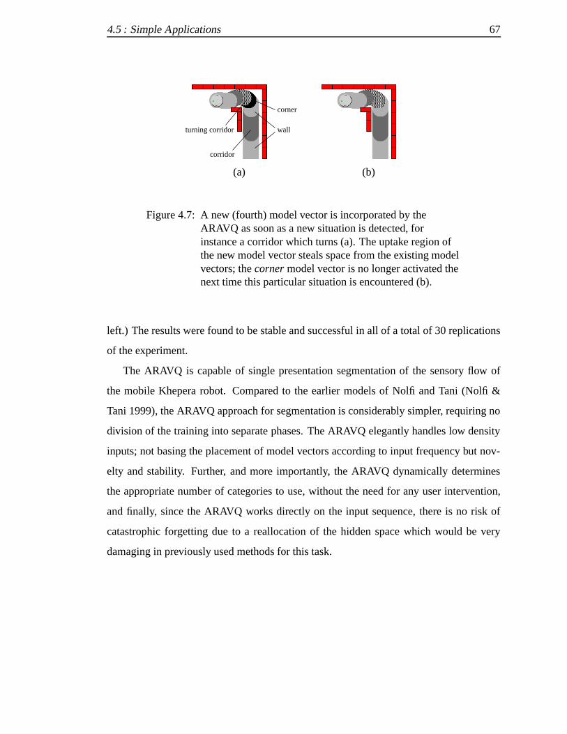
4.5 : Simple Applications 67
turning corridor
corridor
corner
wall
(a) (b)
Figure 4.7: A new (fourth) model vector is incorporated by theARAVQ as soon as a new situation is detected, forinstance a corridor which turns (a). The uptake region ofthe new model vector steals space from the existing modelvectors; thecornermodel vector is no longer activated thenext time this particular situation is encountered (b).
left.) The results were found to be stable and successful in all of a total of 30 replications
of the experiment.
The ARAVQ is capable of single presentation segmentation of the sensory flow of
the mobile Khepera robot. Compared to the earlier models of Nolfi and Tani (Nolfi &
Tani 1999), the ARAVQ approach for segmentation is considerably simpler, requiring no
division of the training into separate phases. The ARAVQ elegantly handles low density
inputs; not basing the placement of model vectors according to input frequency but nov-
elty and stability. Further, and more importantly, the ARAVQ dynamically determines
the appropriate number of categories to use, without the need for any user intervention,
and finally, since the ARAVQ works directly on the input sequence, there is no risk of
catastrophic forgetting due to a reallocation of the hidden space which would be very
damaging in previously used methods for this task.

4.6 : Discussion 68
4.6 Discussion
A novel variant of Leader was introduced, an Adaptive Resource-Allocating Vector Quan-
tiser (ARAVQ), which manages to avoid the spurious experts which would be incorpo-
rated by the earlier Leader algorithms. The ARAVQ incorporates experts quickly, using
a single presentation of the input sequence, and can fine-tune existing experts each time
they re-occur. It can work directly on the input signal, thereby no longer requiring a re-
mapping of the input signal, nor a division of the learning processing into different phases,
which might be necessary in error minimisation-based event extractors. The ARAVQ’s
performance was compared against another recent event extractor, and it was shown that
the ARAVQ could�� capture underrepresented clusters,�� learn the same segmentation
in a mere fraction of time, and�� swiftly learn newly introduced situations (warranting
new experts) in an on-line manner, which were not correctly captured by the existing
technique. In the next chapters, we employ our new data reducer to the memorisation
problems of Route Learning, Novelty Detection, and finally The Lost Robot Problem.
We then move on to learning, and the Road Sign Problem.

Chapter 5
Memorisation Problems
�ROM THE STEADY FLOW of incoming sensory readings, a sequence of events is
extracted by the event extractor. The resulting event sequence can be thought of as
a reduced sensory flowrepresentation as it captures the main characteristics of the signal,
but details about particular input patterns have been filtered out. We here look at how
these reduced sensory flows can let us handle Route Learning, Novelty Detection and the
Lost Robot Problem1.
5.1 Reduced Sensory Flows
As discussed, the memory capacity of mobile robots is often very limited due to en-
ergy consumption and size constraints so storing all individual inputs for future refer-
ence may be very difficult. Even if they could be stored explicitly, finding therele-
vant information—for tasks like environment identification and environment modifica-
tion detection—among hundreds, or thousands, of stored inputs is an intractable task.
Instead of storing each individual input, the inputs can be filtered and a very compact
reduced representation can be stored of the entire input sequence. The idea is captured in
Figure 5.1.
That is, instead of storing each and every input, i.e. aclock based segmentation, see
1Much of this chapter has been published in Lin˚aker & Niklasson (2000a) and Lin˚aker & Laurio (2001).
69

5.1 : Reduced Sensory Flows 70
[0.8 1.0 0.5 0.5 0.9 0.0]
[0.0 1.0 0.5 0.5 0.9 0.0]
[0.1
1.0
0.5
0.5
1.0
0.0]
[0.0 0.0 0.5 0.5 0.0 0.0]
[0.0 1.0 0.5 0.5 1.0 0.0]
[0.7 1.0 0.5 0.5 1.0 0.0]
[0.1 1.0 0.5 0.5 1.0 0.0]
[0.0
1.0
0.5
0.5
0.9
0.0]
[0.1
1.0
0.5
0.5
1.0
0.0]
[1.0 0.9 0.5 0.5 1.0 0.0]
[0.1
0.9
0.5
0.5
1.0
0.0]
[0.1 1.0 0.5 0.5 0.9 0.1]
[0.0
0.9
0.4
0.6
0.9
0.0]
[0.0
1.0
0.5
0.5
0.9
0.0]
[0.0 0.9 0.5 0.5 1.0 0.1]
[0.0 1.0 0.5 0.5 0.9 0.1]
[0.0 0.9 0.5 0.5 1.0 0.0]
[0.0
1.0
0.5
0.5
1.0
0.1]
[0.0
0.9
0.5
0.5
0.9
0.1]
[0.0
0.9
0.5
0.5
1.0
0.1]
[0.0 0.9 0.5 0.5 0.9 0.0]
[0.1 0.9 0.5 0.5 1.0 0.0]
Robot
[0.1 1.0 0.5 0.5 1.0 0.1]
[0.1 0.8 0.3 0.7 0.2 0.0]
[0.0 0.8 0
.2 0.7 0
.5 0.1]
[0.0
0.8
0.3
0.7
0.7
0.0
]
[0.0
0.7
0.2
0.7
0.6
0.1
]
[0.1 0.8 0.3 0.7 0.1 0.0]
[0.0
0.8
0.4
0.6
0.9
0.0
]a
a
a
c
a
a
a
a
b
b
b
a
a
a
a
a a a a a a d
Robot
d dd
dd
a
d
a
c
a
b
a
Robot
d
(a) (b) (c)
Figure 5.1: (a) The multidimensional sensory input arriving at eachtime-step. (b) An unsupervised event extractor assignseach input to one of its experts, i.e. a spatial filtering. (c)Repetitions of expert assignments are removed and onlythe transitions remain, as events, i.e. a temporal filteringtakes place.
Figure 5.2(a), the system could extract a more compact representation of the environ-
ment2, using anevent based segmentation, see Figure 5.2(b), a distinction put forth in
Mozer & Miller (1998).
That is, as long as the current input matches the current extractor expert (see Chap-
ter 3), a duration counter is simply increased, but if another (possibly even new) expert
matches the input, an event is generated and the counter is reset in order to count the
number of repetitions3. This process enables the system to just store expert use (i.e. a
sort of quantisation) and some counters, something which normally can be done withfar
less space than the individual inputs. This is analogous to the use of a counter in Nolfi
& Tani (1999) to provide their higher level prediction network with more information,
2Here assuming that the inputs only depict the doorway time-steps 16 to 24; this is not the case with theactual robots used in the following simulations and experiments as they have sensors on the front-end sideswhich start to detect signs of the doorway several time-steps in advance.
3This is analogous to atimed event sequence(Cassandras 1993) in DES, but here times are specifiedrelative to each other rather than as absolute time points.

5.2 : Route Learning 71
0 4 8 12 16 20 24 28 32 36 40time step
(a) Clock based segmentation����������������������������������������
(b) Event based segmentation��������
Figure 5.2: Clock basedvs.event based segmentation of the inputsfrom this corridor.
while Nehmzow (2000) used a similar counter to differentiate between walls of differing
lengths in a localisation task.
DEFINITION A REDUCED SENSORY FLOWconsists of a sequence of events, ex-
tracted from the input signal; duration counts for these events may also
be included.
The reduced sensory flow is effectively a lossyrun-length encodingof the underlying
sensory stream. In the following, three applications are presented for reduced sensory
flows: Route Learning, Novelty Detection and dealing with the Lost Robot Problem.
During the presentation of these tasks, effects of different event extractor configurations
are also shown and properties of the extracted event sequences (reduced sensory flows)
are presented.
5.2 Route Learning
Letting a robot run around in an environment, the event extractor produces an reduced
sensory flow representation of what it has encountered along its route. We here look at
what is contained in such a reduced representation, i.e. to which degree it has actually
captured the structures. This is done by looking at the individual experts which are formed
during the route, as well as the sequence in which they are used. The presented technique

5.2 : Route Learning 72
for analysing the extracted experts uses a simple inversion of the robot’s sensory and
motor systems. We also show how this technique can be used to construct crude maps
from just the reduced description of the sensory flow.
5.2.1 Memorised Route Visualisation
If the agent was let loose to explore the environment, and thereby form a set of experts
on its own, it would be of great value to have a mechanism by which the experts could be
analysed. A simple approach would be to manually observe when the different experts are
employed by the agent. We here show that instead of waiting for the agent to (by chance)
encounter a situation which corresponds to a certain expert, we can directly display the
expert using an inversion of the agent’s motor and sensory systems. That is, we display the
perceptions and actions the agent has associated with the expert. We also show that this
technique in fact can be used to construct global maps using just the very compact reduced
sensory flow. These global maps can be used as validation that the reduced sensory flow
correctly has captured structures which indeed are present along the route, and that no
important information has been lost during the mapping to the reduced representation.
In particular, we here present a technique for analysing the experts of an ARAVQ. The
technique is based on the property that the ARAVQ places model vectors, representing
the different experts, directly in input space. This is a unique property of the ARAVQ
which is not present in Nolfi and Tani’s systems (Tani & Nolfi 1998, Nolfi & Tani 1999),
i.e. the inversion techniques presented here are not directly applicable to their system,
unless some sort of ANN inversion technique is applied, like that presented by Jacobsson
& Olsson (2000).
5.2.2 Experiments
In order to show how the ARAVQ is able to adapt to routes (input signals) of differ-
ing complexity, a set of environments were designed using the Khepera Simulator 2.0

5.2 : Route Learning 73
(Michel 1996), see Appendix B for settings. (The simulator was extended with an im-
plementation of the ARAVQ and with some additional plotting functionality.) The en-
vironments differed with respect to overall size and the amount of motor control needed
to guide the robot around the environment using a wall-following behaviour. After some
initial experiments, the following parameters were found to provide an adequate4 segmen-
tation: Æ � �� , � � �� , � � and� � � �. These parameter settings were used in
all of the following experiments, in order to show how the ARAVQ is able to adapt on its
own, without external influences or guidance (such as providing information about how
many different experts the segmentation should be based on).
The input vector consisted of ten sensor values: eight distance sensor readings and two
motor readings. This meant that the ARAVQ had a total of 100 input units (������ � �
and � � ). All values were normalised (linearly scaled) to the range � � �� � before
they were fed as input. As mentioned previously, the Khepera simulator was extended
with additional plotting functionality, namely the capability to plot the winning model
vector (expert) in each time-step. Each model vector was assigned a different colour
(corresponding to different shades in the following pictures), and a large circle was drawn
behind the robot in each time-step, using the colour of the winning model vector. The
segmentation of a simple rectangular-shaped environment is shown in Figure 5.3.
The wall-following controller used in these experiments was a very basic system im-
plemented as in Figure 5.4. The Khepera distance sensors give integer readings between
� � ���, where 0 corresponds to no object present within sensor range, and 1 023 corre-
sponds to an object being very close to the sensor. The two motors can be set indepen-
dently to integer values between [-10,10], where positive values make the wheel rotate in
forward direction.
Any ‘peculiarities’ of the wall-following behaviour show up in the segmentation; this
particular wall-follower implementation tends to over-steer when it encounters corners,
4In these experiments, we were mainly concerned with how well the segmentation captured the mainfeatures of the environment, i.e. whether a global map could be reconstructed from the segmentation. Asdiscussed in the previous chapter, the definition of agood segmentation must be in relation to whetherit (quantitatively) improves the performance, or fitness, of the robot in relation to a task; not just for theevaluation of an external observer.

5.2 : Route Learning 74
Figure 5.3: Segmentation acquired using the ARAVQ and a simplewall-follower which guides the robot (counter-clockwise)along the wall. The ARAVQ has automatically allocatedthree model vectors (experts) for this particularenvironment (represented here by different shades).
left motor right motor
1
23 4
5
6
78 } motor[LEFT] = motor[RIGHT] = 5; /* move straight ahead */else {} motor[RIGHT] = 2; motor[LEFT] = 5; /* losing wall, adjust right */else if (sensor[6] < 300) {} motor[RIGHT] = 5; motor[LEFT] = −2; /* wall too close, turn left */if (sensor[5] > 300) {/* Right wall follower */
Figure 5.4: Code for the simple wall-follower.
which requires the robot to turn to the right to not lose contact with the wall after the turn
(this is why the blackright adjustsegments occur after the corners in Figure 5.3).
An interesting property of the ARAVQ is that it places its model vectors directly in
input space. This is not the case for, e.g., Nolfi & Tani (1999) where the model vectors,
or ‘prototypes’, are placed in the hidden activation space of an ANN prediction network.
That makes their system sensitive to reallocations of the hidden space which occur when

5.2 : Route Learning 75
the system is learning. That is, prototypes which remain in their previous location will be-
come invalid as the inputs which they originally corresponded to may have been mapped
somewhere else in hidden activation space. As we show in the following, this ARAVQ
property of placing the model vectors directly in input space, allows the analysis of the
experts, based on an inversion of the robot’s sensor and motor systems.
5.2.3 Expert Inversion
As depicted in Figure 5.3, the ARAVQ detected three novel and stable types of inputs in
the sensory flow, and it assigned a model vector (expert) to each of them. The extracted
model vectors are shown in Table 5.1. The values were truncated to two decimal digits,
for presentational purposes. Also, for convenience, the model vectors have been labelled
alphabetically in all of the following pictures, instead of �, �, �, etc.
Table 5.1: The extracted model vectors for the environment inFigure 5.3. The first eight values correspond to the eightdistance sensors, the ninth value to the left motor sensorand the tenth value to the right motor sensor.
extracted model vectors
� 0.00 0.00 0.00 0.00 0.19 0.99 0.00 0.00 0.74 0.74� 0.00 0.00 0.00 0.00 0.03 0.31 0.00 0.00 0.75 0.64� 0.00 0.00 0.00 0.06 0.91 1.00 0.20 0.19 0.40 0.75
The extracted 10-dimensional model vectors can be de-normalised (Figure 5.5, left)
to get the actual sensor readings and motor commands for the expert. By analysing the
sensors, and building a distance-vs.-activation table, we can find out which distance a
sensed obstacle needs to be at, in order to produce a given activation on the sensors. This
table can then be inverted in order to find the appropriate distance to the wall when we
have a given sensory activation, as is the case with our model vectors. That is, we can plot

5.2 : Route Learning 76
the location where walls ‘ought’ to be, given a certain activation pattern on the sensors.
How this may look is shown in Figure 5.5 (middle). This particular expert seems to
correspond to the agent encountering a corridor. (The figure actually depicts the inversion
of extracted model vector� from the segmentation in Figure 5.10, below.)
de-normalisation sensor inversion motor inversion
Figure 5.5: Input space model vectors are de-normalised, the sensorsare inverted to find the corresponding environment, andthe robot is then moved according to the motor activations;here it has been moved for 30 time steps.
Further, since the model vectors also contain the motor commands, or, more ac-
curately, the activations of proprioceptive motor sensors, at the time where the expert
was ‘active’, the robot can actually be put into motion. (The model vectors, when de-
normalised, provided continuous values rather than discrete integer values. The continu-
ous values were used in these experiments, for greater accuracy.) Figure 5.5 (right) shows
how a simulated robot can be moved according to the extracted motor activations; in each
time-step the corresponding environment from the sensor inversion is plotted to provide
a space-time representation of the extracted model vector. (The gray trail represents the
path the robot has taken.) A lap in the environment corresponds to the reduced sensory
flow depicted in Table 5.2: 169 time steps where model vector� was the closest match,
followed by 26 time-steps of�, 14 of�, 17 of�, etc.
Using this reduced sensory flow with the sensor and motor inversions of each expert
(plotting the environment for each time-step and moving the robot), a simple global map
of the environment can be reconstructed (Figure 5.6). The robot starts out in the bottom

5.2 : Route Learning 77
Table 5.2: The extracted sequence of model vector winners for one lapin the environment in Figure 5.3, using the extracted modelvectors shown in Table 5.1.
extracted reduced sensory flow
����
�������������������������
���������������������
left corner, where it also ends up, having moved counter-clockwise through the (recon-
structed) environment.
Figure 5.6: Reconstructed global map using the reduced sensory flowfor thesecondlap and the inverted sensor and motorsystems.
A lap in the original environment (Figure 5.3) corresponded to about 702 time-steps.
The reduced sensory flow represents this using just 16 ‘symbols’, i.e, the compression
ratio is roughly 44:1. A remarkable feature is that the robot actually ends up where it
‘ought’ to be, i.e. back at the beginning, even though it has been moved during inversion
for 702 time-steps without any positioning information. This was, however, not the case
during the first lap, in which the ARAVQ actually missed the first corner, but the ARAVQ

5.2 : Route Learning 78
has soon incorporated acorner expert which is fine-tuned by adaptation in subsequent
encounters (Figure 5.7). The first encounter with a corner was here missed by the system
(segmentation shown at top); it was not stable enough and was thus treated as noise. The
ARAVQ immediately incorporatesright adjustat the first encounter (it is both stable and
novel) and detects thecornerfirst at the second encounter (top right corner in the world).
This has a dramatic effect on the reduced sensory flow where sharp corners are captured
correctly as soon as the ARAVQ has allocated a model vector for such inputs.
Figure 5.7: Reconstructed global map using the extracted sequence ofmodel vector winners for thefirst lap and the invertedsensor and motor systems.
If the robot instead is placed in a simpler, circular environment (Figure 5.8), the AR-
AVQ adapts to the inputs and allocates just a single expert (Table 5.3); which is all that is
needed in order to provide a good account of what is going on (Figure 5.9).
Here, a single lap in the original environment corresponds to about 850 time-steps,

5.2 : Route Learning 79
Figure 5.8: A very simple circular environment.
which are represented using a single ‘symbol’ in the reduced sensory flow. In practice,
this means that the sequence of experts will beemptysince an expert label is only printed
onceanotherexpert is the winner; something which will never happen. That is, the expert
label� will never be printed; the counter for the expert as a winner can be considered to
be.
A more complex environment is reflected by the incorporation of more experts. Fig-
ure 5.10 shows such an environment, in which the ARAVQ allocates 5 different experts
(Table 5.4).
Inversions of each of the 5 experts from the environment in Figure 5.10 are displayed
in Figure 5.11. The characterisation of model vector�, here described asleft turn (ending)
is made difficult by the fact that it does not only appear in one context; it actually appears
on its own in the reduced sensory flow, without theleft turn (beginning)expert.
The complexity of the environment or route is also reflected in that the length of the
reduced sensory flow is quite long; in this world, 45 ‘symbol’ instances were used to
describe a single lap (Figure 5.12). The inversion procedure shows (Figure 5.13) that
the extracted model vectors, and the sequence of winners, have captured the structure of

5.2 : Route Learning 80
Table 5.3: The single model vector that the ARAVQ allocates for thecircular environment in Figure 5.8. This single expert willconstantly be the winner.
extracted model vectors
� 0.00 0.00 0.00 0.00 0.24 0.99 0.00 0.00 0.72 0.75
extracted reduced sensory flow
��
Figure 5.9: The reconstructed circular environment using the modelvector from the first lap; for presentational purposes weshow only 900 inverted steps using this model vector. Therobotshouldhave needed only 850 time-steps for a singlelap; the model vector is adapted during subsequent laps tocapture this.

5.2 : Route Learning 81
Figure 5.10: A quite complex environment which will generate manydifferent input patterns in the sensory flow.
Table 5.4: The 5 model vectors extracted from the environment inFigure 5.10.
extracted model vectors
� 0.00 0.00 0.00 0.00 0.09 0.75 0.00 0.00 0.75 0.75� 0.00 0.00 0.00 0.00 0.01 0.26 0.00 0.00 0.75 0.61� 0.00 0.04 0.99 1.00 0.99 0.81 0.06 0.00 0.40 0.75� 0.00 0.00 0.01 0.11 0.94 1.00 0.23 0.20 0.40 0.75� 0.99 0.55 0.00 0.00 0.09 0.78 0.00 0.00 0.75 0.75
the environment in quite striking detail. Again, in the simulated movement, the robot
actually ends up in approximately the correct position, even though it has been moved for
1 866 time-steps without any odometry or global positioning information. This is partly
due to the fact that the motor settings have been smoothed and averaged in the ARAVQ
extraction, and that no noise was applied to the ‘imaginary’ movement. The reduced
sensory flow that the ARAVQ has extracted has accurately captured the structure of the

5.2 : Route Learning 82
� � � � �
Figure 5.11: Each of the 5 experts from the environment inFigure 5.10, sensor inverted (top), and also with motorinversion (bottom). The robot faced forward and has thenbeen moved for 20 time-steps for each expert duringmotor inversion. The experts can be described as follows:wall, right turn, left turn (beginning), left turn (ending)andcorridor.
environment; a lap in the environment depicted in Figure 5.10 is originally about 1 866
time steps, and the reduced sensory flow only contains 45 ‘symbols’, i.e. the compression
ratio is roughly 41:1.
The reduced sensory flow corresponds to the sequence of experts. Each time another
expert is chosen, compared to the previous time-step, another piece gets added to the
reduced sensory flow. Generally, the greater the number of experts which the system has
incorporated, the greater the probability that another expert will be the winner. This is
because all experts share the same (input) space. If an additional expert is incorporated, it
unavoidably will need to ‘steal’ space from the other experts, space which previously led
to them being the winner for that input. This also has another side effect, namely that as

5.2 : Route Learning 83
extracted reduced sensory flow
����
������������������������������������
������������
�������
���
����������������
���������������������������
�����
���������
�����������������
Figure 5.12: The complexity of the environment in Figure 5.10 isreflected in that a single lap needs 45 winners in order tobe stored.
Figure 5.13: The reconstructed environment shows that the extractedmodel vectors and the winner sequence, of the third lap,have managed to capture the environment’s structure to astriking degree.
new experts are incorporated, previously encountered situations may be treated differently
the next time they are encountered; they are seen ‘in a new light’. Compound experts such
as turning in a corner can be split into two separate experts such aswall appeared in front
and turning left and walls to the front-right, if one of these is encountered on its own,

5.2 : Route Learning 84
without the other (provided that it also is novel and stable enough for incorporation). No
experts are ever removed in the ARAVQ; once something has been encountered which is
novel and stable, it is incorporated into the system as an expert and remains there, awaiting
any future occurrences. In this manner, the robot does not need to re-learn inputs it has
once been able to handle, but is able to draw on whatever associations had been made on
previous encounters, no matter how long ago they actually occurred.
5.2.4 Limitations
The presented sensory-motor inversion implicitly assumes that the inputs of each expert
are homogenous to a certain degree so that a single point represents them all adequately.
What happens if the inputs for the expert have a multi-modal or non-uniform distribu-
tion? The corners represent one such situation. Inputs belonging to this expert are not
uniformly distributed across the uptake region; they are in fact sequentially ordered as
going from activation to the front and side sensors, to activation on the back sensors as
the corner is traversed. One way to improve this would be to use a sequential repre-
sentation inside each expert, to capture the sequential nature of the inputs. A different
inversion procedure would then have to be constructed, which is able to re-trace this tra-
jectory. Another alternative would be to represent the inputs differently, e.g., mapping
them onto a directional and velocity vector. That would assume that the signal had a con-
stant change during different periods. Or, as mentioned above, the expert could simply be
split into several ones, thereby achieving an individually higher matching, and inversion,
performance. The ultimate question, however, is whether we reallyneeda high granular-
ity for corners; why should we want it at all? In the current experiments, we wanted to
get ‘crisp’ representations that could be inverted to a map of the travelled route, to show
that the route indeed had been learnt to some degree. In coming chapters, we will look
at filtering of the extracted event streams, where ‘irrelevant’ data will be removed. This
will be based on feedback based on a specific learning task; details are to be found in later
chapters.

5.3 : Novelty Detection 85
5.2.5 Summary
We have here presented a technique for analysing routes, extracted and stored as reduced
sensory flows. This was previously done by trying to manually correlate model vector
winners with a distal observation of the agent’s behaviour, see, e.g., Nolfi & Tani (1999).
We have shown that by ‘inverting’ the robot’s own sensor and motor systems, a relatively
unbiased interpretation of the agent-environment interaction can be obtained. The in-
version shows how the agent perceives the environment through its own ‘eyes’ (sensory
systems) and also shows which actions the agent associates with the different situations.
The experts which are extracted by the ARAVQ capture a remarkable amount of infor-
mation about the environment’s structure along the route. In fact, global maps can be
extracted from the reduced sensory flows which the ARAVQ produces, even though the
inputs to the sensory flows by themselves contain no positioning information whatsoever.
This property instead emerges from the agent-environment interaction which underlies
the sensory flow.
5.3 Novelty Detection
This second set of memorisation experiments deals with a system for detecting different
types of changes in a mobile robot environment. The system uses the reduced sensory
flow representation as a compact event based reference representation of the robot’s en-
vironment, of how itshouldlook. The reference representation is then used during patrol
to detect deviations such as doors having been previously open but now closed, moved
objects, shortened or extended corridors, widened openings, etc. All these situations lead
to the incoming sensory patterns during patrol not matching the stored reference repre-
sentation, and thus the robot can alert security. This is similar to the approach in Nolfi &
Tani (1999), but we provide a more thorough look at the different types of modifications
that can be detected, do it with real robots as well as in simulations, show how the system
can benefit from adding reference points in the environment, making it possible to detect
minute changes in the surroundings.

5.3 : Novelty Detection 86
5.3.1 The Problem
Consider a small automated robotic vehicle which travels the corridors of a high-security
building. The robot monitors the environment, matching incoming sensor readings with
stored representations of how itought to look, and quickly alerts security in case a sig-
nificant mismatch, or change, has been detected. One important part of this monitoring
system is the ability to detect novel input patterns, i.e. inputs which do not match any-
thing previously encountered. This is commonly referred to asNovelty Detection, which
for instance can be implemented using very simple habituating Self-Organised Maps like
that presented in Marsland et al. (2000). Detecting ‘unusual’ inputs constitutes only a
small part of what the monitoring system needs to be able to do. In the following, we
present a look at several different types of modifications that all could be considered as
‘novel’.
5.3.2 Environment Modifications
Note that before the monitoring can take place, the robot needs to build some sort ofref-
erence representationof the environment, depicting how itshouldappear during patrol.
That is, the robot should learn what a ‘normal’ environment looks like. When set intopa-
trol mode, the robot should then report any significant deviations from the norm. Different
examples of changes to the environment, all of which the robot should be able to detect,
are shown in Figure 5.14. As we will show, the nature of the reference representation is
influenced by the sorts of changes we require that the robot should detect.
The simplest case is that of detecting new ‘types’ of inputs, or what we callType
Noveltydetection, i.e. inputs which have never been encountered during training. An
example is shown in Figure 5.14(a), where only one type—or ‘expert’ as we will re-
late these to in the following—namelycorridors, has been encountered during training,
whereas two input types,corridorsanddoorways, are detected during patrol. These sorts
of changes can be detected by simply storing as a reference representation the set of input
types encountered during training. When patrolling, the inputs are matched (with some

5.3 : Novelty Detection 87
reference patrol reference patrol
(a) Type Novelty (b) Type Absence
reference patrol reference patrol
(c) Instance Novelty (d) Instance Absence
reference patrol
(e) Instance Modification
Figure 5.14: Different types of environment modification. Cases (a)through (e) require increasingly complex referencerepresentations in order to be handled by the system.
tolerance for noise) against this set; if the input is not similar to anything in the reference
representation, the robot sets off the alarm.
Similarly, removal of an input type constitutes the problem of what we callType Ab-
sencedetection. This is depicted in Figure 5.14(b) where the reference representations
would contain open doorways but none are encountered during patrol. The habituation
mechanism described by Marsland et al. (2000) would not, for instance, detect this as it
has no mechanism for actually detectingmissinginputs. This could, however, be achieved
by again storing all known (expected) input types and comparing against the encountered,
but with some added complications such as determining exactly at what point the input
type should be deemed as missing, as it might very well be encountered at the very next
time-step, or the one following that.
A somewhat more difficult task, which also is difficult to achieve using just a habituation-
based system, is that ofInstance Noveltydetection, i.e. detecting whenadditional inputs

5.3 : Novelty Detection 88
from a type have been inserted, see Figure 5.14(c). The reference representation would
need to contain the expectednumberof inputs for each input type. (Such a system would,
however, not detect if the inputs where ordered differently, e.g., one long doorway could
have been replaced with two smaller doorways at different locations.) Similarly,Instance
Absencedetection implies that the system should be able to detect when the number of
inputs for any of the types has decreased during patrol, as is depicted in Figure 5.14(d).
Even more difficult is the situation where the robot should be able to detect when
something in the environment has changed position—or been otherwise changed—what
we call Instance Modificationdetection. One such situation is depicted in Figure 5.14(e)
where the door which was open during training has been closed but an adjacent door has
been opened instead. To detect such occurrences, the reference representation needs to
contain the actual points in space (or time, as we will show) at which the inputs should
occur, again simultaneously coping with noise, occurring due to sensory fluctuations and
wheel slippage.
5.3.3 Reference Representations
The complexity of the reference representation determines the types of changes which
the system is able to detect, the most complex change being that ofInstance Modifica-
tion. In order to cope with these sorts of modifications, the system needs to store a quite
detailed picture of the inputs which should be expected at each time-step. Clearly, storing
all individual inputs associated with, say one lap in the environment as a reference rep-
resentation, and directly checking input-for-input during patrol, will not suffice. This is
because on the next lap, the individual inputs will be different both due to sensor noise
and because of wheel slippage, inputs may be skipped, or inserted. We here constrain
ourself to only looking at environments in which the robot can do wall-following around
the perimeter, as this provides a systematic and reproducible account of the environment.
The event based segmentation provides a natural solution to dealing with the prob-
lem. Theexpertsdirectly correspond to the different inputtypesdiscussed in the previous
section. Coping with removed or inserted inputs of the same type, can be done by letting

5.3 : Novelty Detection 89
input segments like��
tolerate matching with a wider set of duration counts during pa-
trol. (For instance, a� � tolerance would allow matching to��
through���
.) Further,
any modifications like widened door openings or position movements, are directly re-
flected in that the duration counts for events have been altered, compared to the reference
representation. Thus, all this requires that the system has the ability to extract an event
based segmentationon-line, i.e. during patrol, and to compare it with the stored reference
representation. The next section describes a set of such experiments.
5.3.4 Experiments
The ARAVQ was set to extract a reference representation of a mobile Khepera robot’s
environment. The simulated version (Michel 1996) of the Khepera robot and the simple
wall following program which controlled it are shown in Figure 5.15. (The distance
sensors have integer valued activation in the range � � ��� and each motor can be set to
an integer value in the range�� � � �.)
left motor right motor
1
23 4
5
6
78
else if (sensor[6] < 800) {
if (sensor[5] > 200) {
} motor[LEFT] = motor[RIGHT] = 5; /* move straight ahead */else {} motor[RIGHT] = 2; motor[LEFT] = 5; /* losing wall, adjust right */
} motor[RIGHT] = 5; motor[LEFT] = −2; /* wall too close, turn left */
Figure 5.15: The Khepera robot and the controller used in theexperiments. The robot has eight distance sensors(labelled 1 through 8) and two independently controlledwheels (the front of the robot is facing towards the top).
A real-world Khepera was also employed in these experiments. The setup consisted

5.3 : Novelty Detection 90
of a 1m by 1m arena with rearrangeable wall segments, thereby enabling modifications
during run-time. One of the used environments is shown in Figure 5.16.
Figure 5.16: One of the used environments.
The Khepera robot was connected to a laptop via a serial interconnect cable with a
rotating contact for free robot movement. The laptop received the Khepera sensor read-
ings in real-time and sent appropriate control commands to guide the robot through the
environment. Initial experiments using the Khepera radio turret were also conducted but
the resulting communication bandwidth was deemed insufficient to accurately guide the
robot in real-time, and thus the serial cable was used instead. The entire setup is displayed
in Figure 5.17.
The eight distance sensor activations and the two proprioceptive sensors for the motors
were normalised to the range � � �� � and fed as a ten-dimensional input vector to an
ARAVQ with the following parameters:Æ � ���, � � �� , � � , and� � � �. As
the robot moved about in the environment, the ARAVQ analysed the inputs, extracted a
set of experts, and used these experts to classify individual inputs. This classification is
shown as a trail in Figure 5.18, where each colour depicts the expert which the input at that

5.3 : Novelty Detection 91
Figure 5.17: The real-world Khepera experiment setup with a laptopconnected via a serial cable.
position was classified as belonging to. The figures in the following display the simulation
segmentation as it would be difficult to produce a similar coloured trail in the real world.
No notable difference was detected in terms of sensory and motor signals between the
real-world setup and the simulator; the exact same control program was employed for
both.
The ARAVQ here extracted three experts, roughly corresponding tocorridors, cor-
ners and doorways. This is because the corners are the only points where the wheel
motors are repeatedly set to different values, and the doorways are the only points where
the left sensors detect no walls, i.e. where they give off very low activations; something
which the ARAVQ swiftly picked up. The extracted event based reference representation
for the environment’s perimeter is shown in Figure 5.19. (As was shown earlier, also
using more complex environments, such a sequence in fact captures the spatio-temporal
characteristics of the underlying sensory flow to a striking degree. In fact, it could be used

5.3 : Novelty Detection 92
Figure 5.18: Segmentation for a counter-clockwise run along theperimeter, using the ARAVQ. The ARAVQ extractedthree experts; in light gray:�, in black:�, and in darkgray: �.
to recreate a picture of the visited part of the original environment.)
reduced sensory flow
���
�������������
�������
�������������������������������������
���������������
Figure 5.19: Reduced sensory flow for one lap in the environment’sperimeter.
Once a reference representation had been extracted, the robot was set intopatrol mode.
During patrol, the sensory inputs were classified using the ARAVQ, and the resulting
reduced sensory flow was compared on-line with the stored reference representation. If a
mismatch was detected, the robot stopped and sounded the alarm. A tolerance of�� �
for the duration counts was used; the standard deviation increased linearly with the length
of the duration counts, see Figure 5.20, and was on average about�� �. A set of different
modifications, shown in Figure 5.21, were tested:

5.3 : Novelty Detection 93
a c b c a c a c b c a c a c a c b c a c a c b c0
50
100
150
200
250
300
350
400
Figure 5.20: Averages and standard deviation for duration counts from100 laps in the environment depicted in Figure 5.18.
� In Figure 5.21(a), the upper left doorway was closed. The system detected this
instance absence as the duration count for the corridor came to exceed the tolerance,
i.e. the doorway did not appear as expected.
� As shown in Figure 5.21(b), the upper right doorway was moved slightly to the
right. This instance modification was also detected as the duration count for the
corridor was now below the lowest tolerance.
� Another doorway was opened in Figure 5.21(c). This instance novelty was detected
as a doorway was not supposed to occur for several time-steps.
� Finally, in Figure 5.21(d), the bottom left doorway was widened slightly, i.e. an
instance modification. Interestingly, the system did not detect that the doorway
began too soon (see below), but it instead did pick up on the fact that the doorway
itself was longer than usual.
The reason that the system did not detect that the doorway in Figure 5.21(d) started
earlier than expected was due to the fact that the duration count for the expert which
preceded it (i.e. the corridor) was very large. This, in turn, made the tolerance increase

5.3 : Novelty Detection 94
(a) Door closed (b) Door moved
(c) Door opened (d) Door widened
Figure 5.21: A set of different modifications to the environment. Therobot correctly detects each situation, stopping where theanomaly is detected, and sounding the alarm.
to a point that the change was within the normal fluctuations. This can be considered as
analogous to the situation where we should determine whether two objects (such as two
doorways) are 101 or 102 meters apart simply by pacing out the distance between them.
The problem is that errors tend to accumulate with distance. Conversely, we generally
have no difficulty in distinguishing if the objects are 1 or 2 meters apart (the same absolute
difference). The reason for this is, at least in part, that the reference points are much
closer, and the errors will not have had the opportunity to accumulate. To test this in
the modification detection system, we introduced another reference point, closer to the

5.3 : Novelty Detection 95
doorway. As shown in Figure 5.22, the original environment was modified to include
another open doorway. This doorway served as a closer reference point, and consequently,
when the robot was again set to patrol the environment, it could now detect earlier that
the doorway had been widened.
(a) New reference room (b) Door widened
Figure 5.22: Example of reference points and detection. The system isable to use the inserted open doorway as a referencepoint and can thus quicker determine that the nextdoorway has been modified.
This indicates that the robot may actually benefit from patrolling inmore complex
environments, i.e. environments which have a more frequent switching of experts, in that
the system can use the expert switches (events) as reference points in order to detect even
smaller modifications, not only quicker, but also more reliably.
5.3.5 Summary
We have shown a simple system for detecting different ‘novel’ configurations of a mobile
robot environment. The system is based on the extraction of an reduced sensory flow
from the continuous-valued input stream. The robot first travels around, using a simple
wall following controller, and records the state of the environment as itshould look.

5.4 : The Lost Robot Problem 96
This reference representationis then used during patrol to detect deviations. We have
shown that the robot can detect a wide variety of modifications such as doors having been
previously open but now closed, moved objects, shortened or extended corridors, widened
openings, etc. All these situations will lead to the incoming sensory patterns during patrol
not matching the stored reference representation, and thus the robot will alert security.
Finally, we also showed that the system can benefit from additional introduced reference
points in the environment, thereby making it possible to detect even more minute changes
in the surroundings.
5.4 The Lost Robot Problem
The third and final robot memorisation task we look at is the Lost Robot Problem. Con-
sider an automated window cleaner which works its way through an office building and
cleans the windows. Each room may have its own cleaning specifications, e.g., windows
in front of the building, near the entrance, should be cleaned more frequently than others.
Personnel may at any time do a manual override and move the robot to their own office,
or any other part of the building, and command it to immediately clean their windows.
When finished, the robot should resume its normal duties. This will, however, require that
the robot finds out where it is in the office environment. This problem is known as the
Lost Robot Problem (Nehmzow 2000). The robot needs to gather evidence about where
it presently is located in the environment.
It may, however, be very difficult to find out where the robot is located based on
the information available from the sensors as the environments can look very similar.
That is, the robot is experiencing the problem ofperceptual aliasing—there are many
different locations in the environment which correspond to any given input. In fact, the
environments may even be so similar that they contain no unique landmarksat all, but
still, the robot should somehow be able to find out where it is located. Taking into account
sensor inputs over a long time, the robot will be able to identify in which environment it
has been placed, as proposed and shown in Nehmzow & Smithers (1991). We here show

5.4 : The Lost Robot Problem 97
a much quicker approach, where an arbitrarily large number of inputs can be taken into
account instead of just a limited (pre-defined) window of past events. The approach for
localisation presented in Duckett & Nehmzow (1996) is also similar to what we will be
doing, as well as the approach for characterising an environment presented in Nolfi &
Tani (1999). However, we use a standard dynamic programming approach instead of a
ratherad hochypothesis matching scheme, and identifymultipleenvironments instead of
just the location in a single one.
Consider the environments in Figure 5.23. Rooms 0, 1, and 2 have corresponding
numbers of short corridors, or ‘doorways’, placed in different locations. Other than this,
there are no unique landmarks in any of the environments; the only way to differentiate
between the different environments is to incorporate sensor readings with long time in
between. Having sensed one of the corridors, it will take at least 130 time-steps (sensor
samples) at maximum speed to move to a location at which the other corridor can be
sensed. (In these simulations the robot is wall following which means that the robot will
in fact not reach the location of the possible other corridor until after 800 time-steps.) If
instead the reduced sensory flow is used, this will involve taking only a handful of past
inputs (events) into account, as shown in the following.
room 0 room 1 room 2
Wall following:800 time steps
At max speed:130 time steps
(Limited sensor range)
Figure 5.23: Three of the environments used in these simulations.

5.4 : The Lost Robot Problem 98
5.4.1 Simulation Setup
An ARAVQ (see previous chapter) was set to segment the incoming sensory flow of
a simulated mobile Khepera robot, thereby creating an reduced sensory flow from the
inputs. The robot was controlled using a fixed wall following behaviour, moving counter-
clockwise around the environment. At each time-step, the sensor inputs of the Khepera’s
eight distance sensors and two proprioceptive motor sensors were normalised to the range
� � �� � and combined into a 10 dimensional vector and fed as input to an ARAVQ. The
robot moved about in the environment and at each time-step, the current (best-matching)
expert was plotted using a colour of its own, making the trail shown in Figure 5.24.
24
a164
a211
a389
a390 c29
24b
b24b24 a385
b
reduced sensory flow for room 1
����
�������
�������
�������
������
���
Figure 5.24: Acquired reduced sensory flow from room 1 aftersegmentation using the ARAVQ.
As discussed in the previous chapters, Tani & Nolfi (1998) used a more complicated
mechanism for extracting these experts, where the user manually had to specify exactly
how many experts the system should extract. The ARAVQ has the advantage of being able
to determine this by itself, depending on the complexity of the input signal. While the
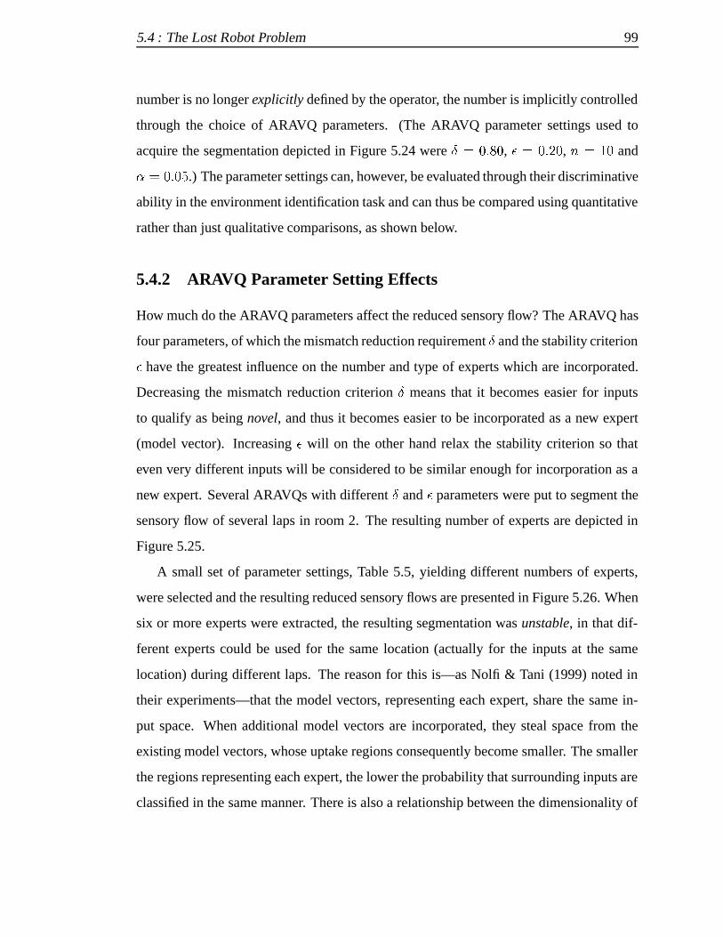
5.4 : The Lost Robot Problem 99
number is no longerexplicitlydefined by the operator, the number is implicitly controlled
through the choice of ARAVQ parameters. (The ARAVQ parameter settings used to
acquire the segmentation depicted in Figure 5.24 wereÆ � �� , � � �� , � � and
� � � �.) The parameter settings can, however, be evaluated through their discriminative
ability in the environment identification task and can thus be compared using quantitative
rather than just qualitative comparisons, as shown below.
5.4.2 ARAVQ Parameter Setting Effects
How much do the ARAVQ parameters affect the reduced sensory flow? The ARAVQ has
four parameters, of which the mismatch reduction requirementÆ and the stability criterion
� have the greatest influence on the number and type of experts which are incorporated.
Decreasing the mismatch reduction criterionÆ means that it becomes easier for inputs
to qualify as beingnovel, and thus it becomes easier to be incorporated as a new expert
(model vector). Increasing� will on the other hand relax the stability criterion so that
even very different inputs will be considered to be similar enough for incorporation as a
new expert. Several ARAVQs with differentÆ and� parameters were put to segment the
sensory flow of several laps in room 2. The resulting number of experts are depicted in
Figure 5.25.
A small set of parameter settings, Table 5.5, yielding different numbers of experts,
were selected and the resulting reduced sensory flows are presented in Figure 5.26. When
six or more experts were extracted, the resulting segmentation wasunstable, in that dif-
ferent experts could be used for the same location (actually for the inputs at the same
location) during different laps. The reason for this is—as Nolfi & Tani (1999) noted in
their experiments—that the model vectors, representing each expert, share the same in-
put space. When additional model vectors are incorporated, they steal space from the
existing model vectors, whose uptake regions consequently become smaller. The smaller
the regions representing each expert, the lower the probability that surrounding inputs are
classified in the same manner. There is also a relationship between the dimensionality of

5.4 : The Lost Robot Problem 100
10−3
10−2
10−1
100
101
10−3
10−2
10−1
100
101
0
10
20
30
40
50
60
70
80
εδ
# ex
pert
s
Figure 5.25: Relaxing the stability criterion (high�) and/or decreasingthe novelty requirement (lowÆ) will lead to an increase inthe incorporation of new experts. (Note the log scale.)
the input space and the number of extracted experts, this relationship is however not com-
pletely straight-forward. The more dimensions there are the greater the potential for more
clusters, but the number of experts extracted from this of course depends on the parameter
settings; a large amount of experts can be extracted from a quite low-dimensional input
space as the input space is continuous-valued, and conversely an input space with a large
number of dimensions can lead to only a handful of experts being extracted depending on
the distribution of inputs as well as the parameter settings of the extractor.
5.4.3 Environment Signatures
How can we evaluate different reduced sensory flows? As discussed, a signature for each
environment can be generated by storing the sequence of experts that are best matches
during one lap. Depending on the parameter settings of the ARAVQ, it may turn out that

5.4 : The Lost Robot Problem 101
Table 5.5: The different parameter settings used in the simulations.
description Æ � �
One expert 0.80 0.01 10 0.05Two experts 0.80 0.10 10 0.05
Three experts 0.80 0.20 10 0.05Four experts 0.80 0.40 10 0.05Five experts 0.40 0.30 10 0.05Six experts 0.20 0.20 10 0.05
these signatures are identical for different environments, see e.g., Figure 5.26 where using
only one expert will make the signatures for all rooms identical. In that case, the room
identification will be impossible.
Once these signatures have been extracted (an example of this is shown in Table 5.6),
they can be used for identification. For the simple environments dealt with here, it is
sufficient to only use the expert information by itself, not their respective duration counts.
If the only difference was in the scaling of different features in the environments (length
of corridors, etc.), such information would, however, be necessary to correctly identify the
environment. Now, if the robot is placed randomly in one of the environments, it should
be able to match its current reduced sensory flow, orevidence sequence, (see Figure 5.27)
with the extracted signatures, and thereby find out where it is.
The environment with the best matching signature is most likely where the robot ac-
tually is. Such a comparison is analogous to a well known and much studied problem
in many application areas: finding the optimal alignment for a pair of sequences. In our
case the problem is complicated by the fact that the evidence can either be an incomplete
sequence ‘taken’ from an already known signature (with the possible added complication
of circular permutation), or be data collected from a previously unseen environment. No
matter the situation, we want the algorithm to find the best alignment between the evi-
dence sequence and any subsequence of the signature sequences. We have now reduced

5.4 : The Lost Robot Problem 102
One expert Two experts Three experts
Four experts Five experts Six experts
Figure 5.26: The extracted sequences where different number ofexperts have been extracted. The number of expertsdepend on the parameter settings of the ARAVQ; see alsoFigure 5.25.
Table 5.6: The reduced sensory flows for one lap in each of theenvironments, extracted using three experts (�, � and�).
extracted reduced sensory flows
room 0 � � � � � � � �room 1 � � � � � � � � � �room 2 � � � � � � � � � � � �

5.4 : The Lost Robot Problem 103
b
a
c
20
201
26
incoming on-line reduced sensory flow
� � � ���
Figure 5.27: Gathering of the evidence sequence. The robot is placedat a random location along the wall in a randomly pickedenvironment and starts wall following in order to gatherevidence of where it is.
the Lost Robot Problem to a level where alocal alignmenthas become applicable; en-
tire environments or rooms can be stored and aligned against each other, or the incoming
(reduced) data.
5.4.4 Local Alignments
The local alignment algorithm5 creates the best possible alignment between subsequences
of the compared pair and if the evidence and signature sequences are identical, the align-
ment will eventually extend to the full length of the sequences. Together with a quantita-
tive scoring method for alignments this gives us the possibility to form hypotheses about
which environment the robot currently is in, and also to detect completelynewenviron-
ments.
5For a review of local alignments, the reader is referred to Durbin, Eddy, Krogh & Mitchison (1998).

5.4 : The Lost Robot Problem 104
Briefly, finding the optimal alignment consists of two parts: An additive scoring
scheme for each aligned symbol vector (with terms for each gap), and a dynamic program-
ming algorithm for constructing the optimal alignment given a specific scoring scheme.
Initial experiments showed that a penalty of 8 for gaps and the following scoring function
for two symbols� and� was adequate:
���� �� �
���
� � � �
�� otherwise�(5.1)
Note that it is possible to have several different alignments that return equal scores. In
order to simplify our analysis of the system we chose to normalise all scores by dividing
them with the maximum possible score for anun-gappedalignment (which would be
obtained if the two sequences were identical).
5.4.5 Results
One example of the alignment technique in action is given in Table 5.7 where the evidence
sequence� � � is gradually aligned to the known environments (rooms 0, 1 and 2) as
the robot moves. When only one event has been observed (in this case the one a distal
observer could denotecorner), it is impossible to know which room the robot is in since
all rooms have corners. Acorner followed by awall is also not enough to discriminate
between the three environments.
It is first when the expert forcorridor is the winning one that it is possible to decide
that the robot cannot be in room 0. The score for room 0 does not go to zero because it
still matches the� �, which is��� of � � �.
In case the signature and evidence signatures do not originate from the same starting
point in the room, we have to be able to handlecircular permutations. We have solved
this by adding at least � � extra symbols at the end of the signature sequences (where
the evidence sequence is of length). These extra symbols are taken from the beginning
from the same signature, when needed, so that we get a sort of wrap-around effect. This

5.4 : The Lost Robot Problem 105
Table 5.7: The normalised matching scores for each environment.
evidence env. matching score
� room 0 � � � � � � � � 1.00room 1 � � � � � � � � � � 1.00room 2 � � � � � � � � � � � � 1.00
� � room 0 � � � � � � � � a 1.00room 1 � � � � � � � � � � a 1.00room 2 � � � � � � � � � � � � a 1.00
� � � room 0 � � � � � � � � 0.67room 1 � � � � � � � � � � 1.00room 2 � � � � � � � � � � � � 1.00
can be seen in Table 5.7 in the form of the non-italic symbols at the rightmost end.
The complete run for one experiment is shown in Figure 5.28, and clearly it is not
possible to discriminate between rooms 1 and 2 until the secondcorridor is encountered.
There is a temporary increase in the score for room 0 as the robot moves along and
this happens because the cost of introducing a mismatch is eventually compensated by
the additional matches which it leads to. As the ninth symbol enters, there is finally a
mismatch in room 1 and consequently the system correctly indicates that the robot is
most likely in room 2 (the only one with perfect match).
Since we normalise the score from the alignment with the maximum possible score,
we can also easily detect new rooms. To show this, room 3 was created with three corri-
dors, see Figure 5.29.
The robot was placed in room 3 and it started comparing its evidence sequence with
the known signatures as it moved. As depicted in Figure 5.29, the scores indicate that
none of the known environments are consistent with the gathered evidence. The overall
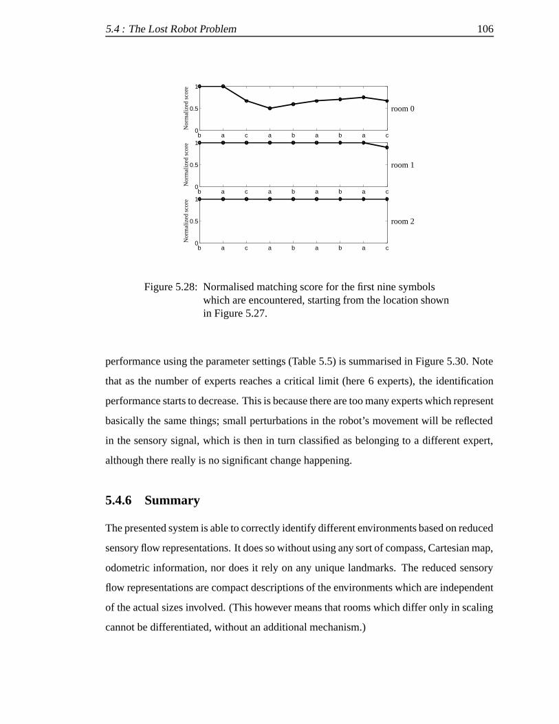
5.4 : The Lost Robot Problem 106
b a c a b a b a c0
0.5
1
room 0
Nor
mal
ized
sco
reb a c a b a b a c
0
0.5
1
room 1
Nor
mal
ized
sco
re
b a c a b a b a c0
0.5
1
room 2
Nor
mal
ized
sco
re
Figure 5.28: Normalised matching score for the first nine symbolswhich are encountered, starting from the location shownin Figure 5.27.
performance using the parameter settings (Table 5.5) is summarised in Figure 5.30. Note
that as the number of experts reaches a critical limit (here 6 experts), the identification
performance starts to decrease. This is because there are too many experts which represent
basically the same things; small perturbations in the robot’s movement will be reflected
in the sensory signal, which is then in turn classified as belonging to a different expert,
although there really is no significant change happening.
5.4.6 Summary
The presented system is able to correctly identify different environments based on reduced
sensory flow representations. It does so without using any sort of compass, Cartesian map,
odometric information, nor does it rely on any unique landmarks. The reduced sensory
flow representations are compact descriptions of the environments which are independent
of the actual sizes involved. (This however means that rooms which differ only in scaling
cannot be differentiated, without an additional mechanism.)
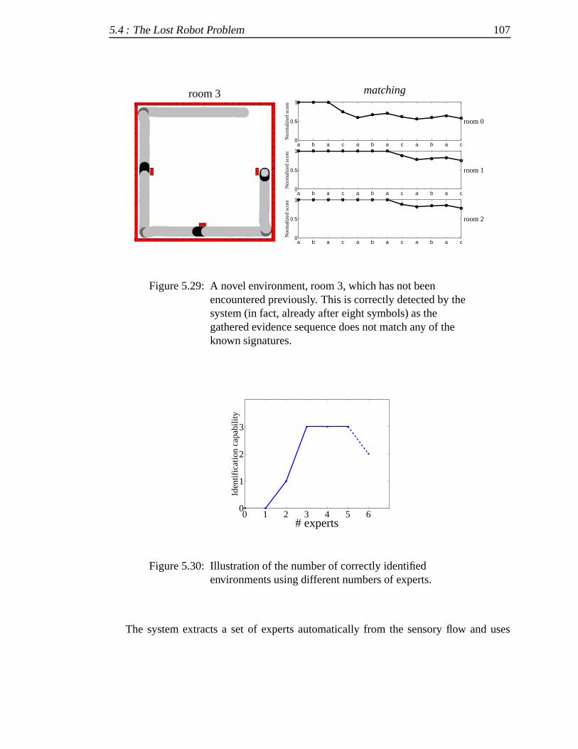
5.4 : The Lost Robot Problem 107
room 3 matching
a b a c a b a c a b a c0
0.5
1
room 0
Nor
mal
ized
sco
re
a b a c a b a c a b a c0
0.5
1
room 1
Nor
mal
ized
sco
re
a b a c a b a c a b a c0
0.5
1
room 2
Nor
mal
ized
sco
reFigure 5.29: A novel environment, room 3, which has not been
encountered previously. This is correctly detected by thesystem (in fact, already after eight symbols) as thegathered evidence sequence does not match any of theknown signatures.
0 1 2 3 4 5 60
1
2
3
# experts
Iden
tific
atio
n ca
pabi
lity
Figure 5.30: Illustration of the number of correctly identifiedenvironments using different numbers of experts.
The system extracts a set of experts automatically from the sensory flow and uses

5.5 : Discussion 108
these experts to create individual environment signatures. These can be matched in par-
allel against a gathered evidence sequence in case the robot gets lost, using a standard
alignment technique. As we have shown, this enables the robot to ‘localise’ itself from
random starting positions and also to detect new environments. The alignment technique
always generates a hypothesis (best matching score) for the evidence, even if there is no
perfect match among the known environments.
The parameter settings of the extraction system will influence the number of experts
formed. This will in turn affect the environment identification performance, and will thus
provide a quantitative measurement of the quality of the parameter settings. The results
show that paying too much attention to details, i.e. having many different experts for
the same thing, may actually hurt performance in a similar manner as having far too few
experts. However, the technique presented here provides help in choosing an appropriate
level of granularity.
5.5 Discussion
In this chapter we have introduced and argued for the usefulness ofreduced sensory flows,
essentially being bottom-up extracted event based representations of an underlying clock
based input stream. They provide a ready means for storing a sensory flow’s main charac-
teristics in a very compact manner; thereby tasks like Route Learning, Novelty Detection
and dealing with the Lost Robot Problem can be performed by simple on-line mechanisms
like the ones presented in this chapter. Properties of the extracted reduced sensory flows,
such as the ‘normal’ variation in duration counts and the effects of different ARAVQ
parameter settings were also investigated. We also showed how to obtain a quantitative
method for determining a suitable granularity (number of experts) for an reduced sen-
sory flow, namely based on overall task performance, e.g., the environment identification
performance impact.
Chapter 6
Learning and Control
�S SHOWN IN THE PREVIOUS CHAPTER, the compact extracted reduced sensory
flows contain most of the information available in the actual continuous-valued,
high-dimensional, time-stepped data stream. Through the use of the ARAVQ, distinct but
infrequent inputs are also included as events. So far, we have focused on the extraction of
discrete asynchronous events from the continuous-valued time-stepped input signal. We
here now start to look at how we can form a control loop by including a set of behaviours
to which different events can be coupled. We discuss different representational levels of
both the inputs and the outputs of the system, and show how the input and outputs can
be coupled in all these levels at once. In this manner, small perturbations or unexpected
signals in input space can be quickly reacted to without the explicit triggering of events to
bring the system back on track, producing a more smooth interaction. A layered system
is built up, which ends up looking much like Brooks’ Subsumption Architecture, but with
some very important differences, like the ability to delegate processing rather than the
former’s more hands-on approach. This gives us the ability to learn, and to completely
automatise tasks on lower layers. In the next chapter, a working implementation of these
ideas is then presented. There, different learners come to master a delayed response task
involving arbitrarily long delay periods; something which is quite impossible at the time-
step level1.
1Most of this chapter has been published in Lin˚aker & Jacobsson (2001b) and Lin˚aker (2001).
109

6.1 : Delayed Response Tasks 110
6.1 Delayed Response Tasks
Events in the real-world domain generally occur on a much slower time scale than that of
individual neuronal and sensory updates. Sampling the environment on the millisecond
level will quickly lead to an intractable amount of data if everything is simply recorded in
memory, especially if the number of sensors is substantial. And, even if the system is able
to store all this data, then trying to make use of it, like trying to find useful correlations
between inputs—and outputs—at different points in time, quickly amounts to a daunting
computational task. A group of problems which are based on finding correlations be-
tween inputs as well as outputs at different points in time are known asdelayed response
tasks. They are characterised by the subject being presented with a stimulus, then a delay
follows, and a cue for responding eventually occurs at which time the subject needs to
act, or respond, based on the stimulus that was presented at the start of the trial. A reward
or punishment is then typically handed out based on performance.
6.2 The Road Sign Problem
In mobile robotics, we can place a robot in the subject’s position. In particular, a problem
known as the Road Sign Problem (Rylatt & Czarnecki 2000) fits this description perfectly.
It is shown in Figure 6.1. In said problem, a robot drives along a road or rolls down a
corridor, sees a road sign (stimulus), continues to travel (delay), until faced with a junction
(cue) at which time the robot needs to decide in which direction to turn (response) based
on the road sign it passed by earlier. The response may not be requested for several
seconds or even minutes, depending on the vehicle’s travelling speed and the distances
involved.
Such tasks are quite common in real-life, involving associations between inputs and
actions at different points in time. Most existing learning methods, like those based on
gradient descent, are however quite inept at handling these sorts of problems. Consider,
for example, a simple approach where a standard neural network is fed sensor activations
through a set of input nodes each time-step. Inside the network, these inputs are put ‘into
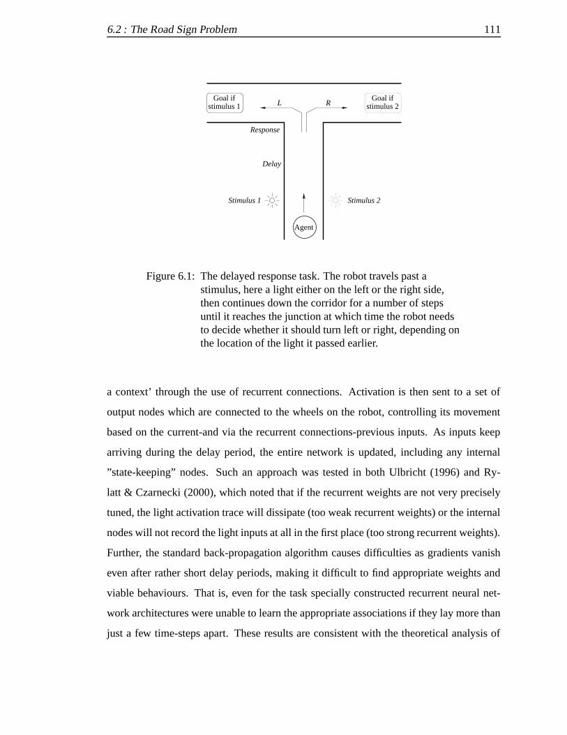
6.2 : The Road Sign Problem 111
stimulus 1Goal if Goal if
stimulus 2
Response
Stimulus 1
Agent
Stimulus 2
L R
Delay
Figure 6.1: The delayed response task. The robot travels past astimulus, here a light either on the left or the right side,then continues down the corridor for a number of stepsuntil it reaches the junction at which time the robot needsto decide whether it should turn left or right, depending onthe location of the light it passed earlier.
a context’ through the use of recurrent connections. Activation is then sent to a set of
output nodes which are connected to the wheels on the robot, controlling its movement
based on the current-and via the recurrent connections-previous inputs. As inputs keep
arriving during the delay period, the entire network is updated, including any internal
”state-keeping” nodes. Such an approach was tested in both Ulbricht (1996) and Ry-
latt & Czarnecki (2000), which noted that if the recurrent weights are not very precisely
tuned, the light activation trace will dissipate (too weak recurrent weights) or the internal
nodes will not record the light inputs at all in the first place (too strong recurrent weights).
Further, the standard back-propagation algorithm causes difficulties as gradients vanish
even after rather short delay periods, making it difficult to find appropriate weights and
viable behaviours. That is, even for the task specially constructed recurrent neural net-
work architectures were unable to learn the appropriate associations if they lay more than
just a few time-steps apart. These results are consistent with the theoretical analysis of

6.3 : From Time-steps to Events 112
Bengio et al. (1994) showing the inadequacy of gradient descent learning of long-term
relationships.
We however note that there is a difference, in terms oflevels of description, between
the task and the low level continuous operating of a robot. The robot will continuously
receive sensor readings, typically in the millisecond range, most of which probably will
be largely irrelevant for the task. Rather than specifying individual actions that the robot
should take at each point in time, the problem is (implicitly) described in terms ofevents.
While the order between events is specified, ‘first the road sign,then the junction’, the
notion of time between the events is not detailed in the task description. That is, the delay
is not limited to always constituting exactly, say,� , or� time-steps. The Road Sign
problem description is thus an account in form of an asynchronousevent stream, while
the operation of the robot sensors and actuators work on a synchronoustime-step based
streamof sensations and actions.
Here we present a quite different approach from Rylatt and Czarnecki, in that we do
not work directly on the input sequence but instead extract a set of events from the inputs
and then we work on this sequence of events. As we will show, the time intervals between
events may in fact be arbitrarily large without affecting the delayed response task learning
in the system; a drastic change from previous approaches. This dramatically reduces the
difficulties of gradient descent learning in this domain. While the event extraction has
been addressed in previous chapters, there now is a new need, namely of gettingback
from an event stream to the level of time-step based inputs and outputs. That is, the
system should be able to use the events to give aresponse; obviously a critical part in any
delayed response task.
6.3 From Time-steps to Events
Event based streams can either consist of manually defined concepts (event types) as in
Mozer & Miller (1998) or extracted bottom-up from an underlying time-stepped stream,
like we have described in the previous chapters. The bottom-up extraction is generally

6.3 : From Time-steps to Events 113
based on having a set of event classes, e.g., realised through a set of experts, into which
individual inputs or input segments can be sorted. The basic idea is that input can be
reduced both spatially and temporally, through a series of processing levels, yielding a
better-suited representation for storage and learning, as depicted in Figure 6.2.
a a a ab a c d e
Classification
aaabbbbbaaaaaaaacccccaaaaddddaaaaaaaaaaaaaaaaaaaaaeeeeeaaaaaa
Event filtering
b d e
Event extraction
Level 4
Level 3
Level 2
Level 1
Figure 6.2: A general view of the four representational levels wepropose for inputs and the bottom-up processes whichinterconnect them. The underlying idea is that higherinformation processing levels are given access tosuccessively longer time horizons through a series ofextraction and filtering stages.
Level 1: Contains raw multi-dimensional sensor data, which is time-step based2. This
is the level where Rylatt & Czarnecki (2000) approached the delayed response task. Find-
ing useful correlations may, however, be very difficult on this level due to large numbers of
input dimensions and large numbers of input samples being received continuously. Like
Nolfi & Tani (1999), we note that real-world task dependencies do most often not manifest
2Where a time-step is defined as a single update of sensors, neuronal elements, and actuators with aregular time interval, typically in the millisecond range.

6.3 : From Time-steps to Events 114
themselves at this level of individual time-stepped neuronal updates, but rather on much
slower time scales, involving several seconds or even minutes. Rylatt and Czarnecki’s
somewhat simplified simulations and a specially modified neural network architecture
was only able to learn dependencies which lay up to 13 time-steps apart. But as most
robot systems have a high sampling frequency, such a system would not be sufficient.
For example, the Khepera robot we use in our experiments, has sensor sampling rates of
approximately 20 times per second. Rylatt and Czarnecki’s system would therefore, in
effect, not be able to learn tasks involving even just single second delays3. In the follow-
ing, we will show that by using event extraction, the delays can instead be arbitrarily large
and this enables the system to handle more realistic long-term dependencies.
Classification: The process whereby the raw multi-dimensional sensor data is divided
into a set of classes based on their matching toexperts; see Chapter 3. While Nehmzow
& Smithers (1991) employed a set of manually predefined (fixed) experts for this, Tani &
Nolfi (1998) instead let the system determine the experts by itself, thereby reducing the
user intervention. However, Tani and Nolfi still had to manually specify the number of
experts, and had to divide the training into several different phases. They also had large
problems with inputs which were distinct but not very frequent in the training set, and
the learning process was very slow. In Chapter 4, a more flexible classification system
was developed, the Adaptive Resource-Allocating Vector Quantiser (ARAVQ). It is able
to swiftly classify inputs using a dynamic number of automatically extracted experts,
overcoming most of the problems in Tani and Nolfi’s system. (The ARAVQ system is the
one used in the following.)
Level 2: Contains raw time-step based multi-dimensional data which have been tagged
with expert labels. If each expert is allotted a character in the alphabet, the input can be re-
written, with some loss of information, as a (very long) letter sequence. This is the level
at which Ulbricht (1996) approached the Road Sign Problem, trying to learn associations
3There is no principal reason why a recurrent neural network could not learn the task at this level, usinga non-gradient descent based weight updater. For instance, in Ziemke & Thieme (in press), weights tohandle this task were obtained through an evolutionary algorithm. However, we are interested in systemswhich can learn the task on-line, using some sort of temporal credit assignment.

6.3 : From Time-steps to Events 115
between the letters in the sequence. She did not, however, provide any account for how
the input had become this letter sequence (i.e. no Level 1 nor any classification), thereby
working on essentiallyungroundedsymbols. Further, as her system was still time-step
based, she had the same difficulties learning long-term dependencies as Rylatt and Czar-
necki had in their Level 1 system, but she had a somewhat more compact representation
to work with.
Event extraction: The process whereby only the transitions between expert mem-
bership of the lower level data are extracted, thereby filtering out repetitions. This is a
fairly straightforward mechanism as long as the expert membership is exclusive (each
input belonging to one—and only one—expert); if two succeeding inputs are classified
differently, an event is generated. The detection of an event generates a signal to the next
level.
Level 3: Contains general events, interspersed over long periods of time. Updates
occur asynchronously on a considerably slower time-scale than the time-step based levels
below it. This means that longer time-dependencies can be detected, as noted by Nolfi &
Tani (1999). While their robot system worked at this level, it did not involve any coupling
back to the real-world as the input was merely classified and repetitions removed, and not
acted upon in any manner. That is, their system did not use the extracted events to control
the robot; it was in fact only an idle observer of what was going on. In the following, we
provide an account for how extracted events can be used to learn delayed response tasks
and also how this can be used to identify candidates which should pass through an event
filtering on to yet another level.
Event filtering: The process which discards events which are considered as irrele-
vant for accomplishing the task. This process requires that the events have been rated
with some sort of ‘usefulness’ score, related to how relevant they are for achieving the
task. This event rating should ideally be based on a delayed reinforcement learning sys-
tem, such as Q-learning, as rewards in the real world do often not come immediately as
an action is performed. Such a delayed reinforcement scheme is constructed in the next
6.4 : From Events (Back) to Time-steps 116
chapter, as well as a simpler, but less realistic, evaluation mechanism based on instanta-
neously rewarded supervised learning. Once a simple version of the task has been learnt
on a low level, it can be generalised to more complex situations on higher information
processing levels that have access to longer time horizons.
Level 4: Contains only the events which are considered relevant for achieving the
task. It is updated on an even slower time-scale than Level 3 and thus can handle events
that have occurred even further apart.
Inputs at Level 1 correspond to individual sensation patterns, whose dimensions and
encoding regimes are determined by the actual sensation subsystems (hardware connec-
tivity). However, Level 2 and upwards do not work on individual sensations, thereby
allowing a completely different encoding regime to be employed. More specifically, on
these levels the system can work on an essentially symbolic representation whose size is
virtually independent of the dimensionality of the actual sensory and motor systems. This
relaxes the information processing and storage demands on the system, assuming that
the ‘symbolic’ representation is more compact than its corresponding inputs or outputs,
which usually is the case.
As we mentioned, just extracting an event based input representation of the task is not
sufficient for handling delayed response tasks; the system needs to be able to produce a
responsebased on the event stream. In the next section, different options are reviewed for
going from the event based level down to concrete actions.
6.4 From Events (Back) to Time-steps
In addition to the information processing capabilities described in the previous section, the
system needs to be able to control the robot, i.e. making the appropriate response once the
cue for responding comes. There are several possibilities of executing actions. Levels 1
and 2 are both time-step based, which means that the inputs can be directly coupled to
a single action which lasts a proportionate single time-step. This can accommodate for
simple, non-goal-oriented, and/or ‘innate’ reflex actions. However, associations between

6.4 : From Events (Back) to Time-steps 117
inputs at Levels 3 and upwards are based on events.
A single time-step action is therefore not appropriate as a response; the response
should ideally affect the performance the entire time interval up to the next event. A
simple solution is to repeatedly execute thesameaction until the next event occurs, e.g.,
to keep turning in one direction until the next event occurs. This would, however, be a
very rigid and inflexible solution, not allowing the system to modify its responses into
smoother real-time interactions. Instead, we propose, to let the event-based levels mod-
ulate the actual input-to-output (sensation-to-action)mappingof the time-step based lev-
els. This modulation also gives the system the ability to focus on particular sensor subsets
which are of most importance to the particular response.
The layered structure of our system is based on the Real-Time Control System (RCS)
architectures; for a review of different RCS versions and implementations see Albus
(1993). Like RCS, we have multiple time-scales or ‘resolutions’ in the system, where
higher layers operate on longer time-scales than lower ones. A difference is that the prim-
itives of each layer are not pre-defined in our system, and the temporal updating may vary
dramatically during a single interaction, as events are triggered asynchronously. In RCS,
task knowledge is manually put into ‘task frames’ which describe all parameters, agents,
goals, objects, requirements and procedures for performing the task. In our system, this
is instead learnt, based on some sort of feedback (see next chapter), and the knowledge is
not explicitly represented and structured in the manner that the RCS frames are.
If we consider the Road Sign Problem, a Level 3 representation is sufficient for most
learning methods. (A Level 4 representation would contain only the stimulus and cue
events.) Going from Level 3 down to Level 1, Figure 6.3, we characterise as follows:
Level 3: An asynchronous specification of the behaviour which is to control or affect
the system’s outputs until the next event occurs. This specification can be the result of a
process which takes several of the previous events into account.
Temporal unfolding: The process which simply repeats the behaviour command to
the lower level. Like the input’s event extraction mechanism, this is a pretty straight-
forward mechanism to implement.

6.4 : From Events (Back) to Time-steps 118
Realisation
Level 3
Temporal unfolding
CCCCCCCCCCCCCCCCCCCCCCCCCCCCCCCCCLLLCCCCCCCCCCC
Level 1
Level 2
corri
dor
junc
tion
Input events
tC C C L C
left
light
corri
dor
corri
dor
alt (i) − specifying
alt (ii) − modulating
Figure 6.3: Behaviours are selected asynchronously on Level 3 andare unfolded onto a Level 2, time-step based,representation. This in turn either specifies or modulatesthe Level 1 actions. Two behaviours were used here: acorridor follower C, and a left wall follower L.
Level 2: A time-step based specification of the behaviour to use at that particular
instance. This specification may either arrive from Level 3 through temporal unfolding,
or it could be specified directly using a mapping from the Level 2 input. The advantage
of coupling it directly with the Level 2 input would be that a response could be generated
quicker since all processing delays associated with Level 3 would be bypassed. A more
general solution would be to generate a response at this level directly when a classification
change occurs on the Level 2 input, but to modify, or correct, it once the more informed
behaviour specification eventually arrives from Level 3.
Realisation: The process whereby a behaviour is set to modify the actual actions
which are to be performed each time-step. The impact of the behaviour on the individual
actions may be more or less specifying (see below).

6.4 : From Events (Back) to Time-steps 119
Level 1: A time-step based specification of the individual output, or action, to take.
There are at least three easily identifiable ways in which this could be determined, namely
using aspecifyingcontroller, areflexivecontroller, or amodulatingcontroller, as de-
scribed below. The latter one being the most flexible.
DEFINITION An ACTION is an output pattern which is sustained for a single time-
step.
A simplespecifyingcontroller would just repeat the same action over and over again
until the behaviour specification changed on Level 2:
�������� � ���������� ����� (6.1)
On the other end of the spectrum, areflexivecontroller would completely ignore the be-
haviour specification and only base its action on the current Level 1 input:
�������� � ������������� (6.2)
In between these extremes, amodulatingcontroller would not specify the exact action
which is to be performed, instead it would only affect the way a direct Level 1 mapping
from sensations to actions was performed. This modulation could be realised through
inhibition or excitation, as to bias the response in some direction. That is, the response
would be generated with both the actual Level 1 sensation and Level 2 behaviour specifi-
cation taken into account:
�������� � ������������� �������� ���� (6.3)
Note that this would allow a response to be generated as soon as an input arrives, as the
processing on Level 2 does not have to be awaited. When the behaviour specification
eventually arrives, it can however be taken into account and the actions can be biased in

6.4 : From Events (Back) to Time-steps 120
(a) (b)
Figure 6.4: When the robot reaches the end of the corridor, it is to turnright and follow the wall. If the turning behaviour isspecified top-down only, ‘keep turning 10 degrees to theright’, the robot may end up crashing into the smallunforeseen obstruction (a). If instead a modulatingcontroller is used, inputs can also be taken into accountdirectly when turning, allowing the robot to make smalland quick adjustments as to avoid the obstacle (b).
some direction.4
A reflexive or ‘reactive’ controller would not be able to learn anything more than
the simplest input-to-output mapping at it does not make use of the available top-down
information. A specifying controller could potentially handle the Road Sign Problem, but
could easily create oscillations and instability in the interaction as small changes in the
input are completely disregarded; only drastic, event-generating, inputs are considered
by such a controller. A modulating controller, would however be able to incorporate the
best of both worlds, i.e. quick modification of its actions and incorporation of top-down
information. An example which shows the advantage of a modulating controller over a
specifying controller is depicted in Figure 6.4.
A specifying controller forces the system to produce a certain output, i.e. how to act,
regardless of the inputs. A modulating controller specifies not the manner in which to act,
but rather the manner in which tointeract. That is, the system outputs continuously affect
4A side-effect of using a modulating controller in a real-time context would be that a fast, or drastic,change in the input would produce a reflex—or innate—Level 1 response if higher levels have not pickedup on some clue from earlier inputs and begun inhibition or excitation in anticipation.

6.5 : Control 121
the environment (inevitable through its own existence therein), and the environment at all
times also affects the system’s outputs.
DEFINITION A BEHAVIOUR is a particular input-to-output mapping which is sus-
tained repeatedly for several time-steps.
Behaviours are sustained until the next event arrives, at which time another behaviour
may be selected. This however means that behaviour shifts can only be triggered by
events, not in the period between events. Note that a behaviour does not by itself specify
any particular action; several behaviours may produce similar actions and a single be-
haviour may produce a wide range of actions as each time step’s action depends on the
input for that time-step. It may therefore be difficult or even impossible to determine
which behaviour is in effect at a particular point in time by only observing the external
outputs (actions) of the system.
6.5 Control
In our system, higher levels do not directly themselves specify actions, unlike layered con-
trol architectures such as Brooks’ well-known Subsumption Architecture (SA) (Brooks
1986). The event-based asynchronous approach presented here will allow adecoupling
of higher layers from the immediate ‘here-and-now’ of sensory-motor processing. Com-
pare this to the more hands-on, do-it-yourself approach of the SA, where the higher layer
itself takes over (subsumes) the output production of the lower layer at various points in
time. This effectively means that all resources of the higher layer are assigned to the im-
mediate control of the system. Our approach instead works bydelegationof work, always
letting the lower layer do the actual processing. The higher layer just specifies theoper-
ating modeof the lower layer from a set of such modes, or a blending thereof. In the next
chapter, three such operating modes (input-to-output mappings) are manually defined in
the lower layer of an event-based control system. We also show how operating modes
instead can be constructed autonomously, and discuss how they can be blended together
6.5 : Control 122
if realised through mappings like neural networks.
A very simple approach—which we will be using—is to implement operating modes
(behaviours) as purelyreactivesystems, working on Level 1 representations. The lack of
internal state might seem very limiting in terms of output production, as there then is no
internal counter or context for progressively executing the steps of an output sequence.
A simple static mapping system can, however, entail for example a cyclic production of
output patterns, as the system is situated in an environment. The system output can be
retained the following time-step through the use of sensors, thereby forming a feedback-
loop or iterated function system. For example, consider a robotic arm equipped with pro-
prioceptive sensors on the actuators. Setting the motors in a particular setting will report
(at least approximately) this particular setting the next time the motor sensor is sampled.
We thereby get a recurrency from the output to next time-step’s input. An example of
such a simple reactive mapping5 is given in Figure 6.5(a). The system will be guided
by the vector field to follow the cyclic trajectory, regardless of starting position (due to
noise this is the only sustainable attractor). One particular evolution of the system for a
couple of time-steps is presented in Figure 6.5(b), and a global picture of the mapping is
presented in Figure 6.5(c). This particular system is even in some sense self-regulating,
or self-stabilising, in that the system automatically recovers from perturbations caused by
external influences, as the field will guide it back to the cyclic attractor. That is, even if
the feedback from the proprioceptive motor sensors does not accurately portray the last
output in a 1:1 manner, the system will still travel along the cyclic trajectory. The same
holds if we perturb or affect the position of the robot arm; again the attractor will guide
the arm back into the cyclic output pattern production.
These sorts of attracting vector fields can be learnt from single trajectory paths, using
for instance gradient descent, as shown by Goerke & Eckmiller (1996). That is, a ‘desired
path’ can be used as a template, and a mapping covering the entire input space can be
extrapolated from this template6. This is a sort of generalisation of an instance.
5This particular network uses a���� output activation function.6A similar idea was presented by Hohm, Liu & Boetselaars (1998). Their system learned to produce
smooth motion trajectories for a task originally specified in the form of rules.

6.5 : Control 123
~1:1
ENVIRONMENT
bias
outputsinputs−0.9
1.00.5
0.7
−0.3
0.2
(a)
−1 −0.8 −0.6 −0.4 −0.2 0 0.2 0.4 0.6 0.8 1−1
−0.8
−0.6
−0.4
−0.2
0
0.2
0.4
0.6
0.8
1
Motor 1 & Sensor 1
Mot
or 2
& S
enso
r 2
−1 −0.8 −0.6 −0.4 −0.2 0 0.2 0.4 0.6 0.8 1−1
−0.8
−0.6
−0.4
−0.2
0
0.2
0.4
0.6
0.8
1
Motor 1 & Sensor 1
Mot
or 2
& S
enso
r 2
(b) (c)
Figure 6.5: A single static input-to-output mapping (a) can lead to thesystem exhibiting cyclic behaviours due to theenvironment acting as a recurrent connection for thesystem. An example trajectory (b), and uniformlydistributed samples (c) of a single mapping step.
The system ends up looking much like a Hybrid Control Architecture, or aswitched
plant (Moor, Raisch & Davoren 2001, Davoren, Moor & Nerode 2002), where a high-
level supervisory controller switches between a finite number of continuous low-level
controllers, all acting on the same physical plant. In such systems, the supervisor acts
on quantised measurement information (events), similar to our approach. An important
difference is however that such control architectures are constructed to satisfy a defined
language inclusion specification, i.e. the ‘desired’ or ‘correct’ operation of the system is

6.6 : Event Representation 124
already known and deviations from that correct operation are assumed to be detectable.
The layered system we suggest can be characterised using the twelve different prop-
erties or dimensions put forth in Sloman (2000). For those familiar with these dimen-
sions, we regard our system as employing concurrent layers, and being predominately
functionally differentiated, with trainable layers, similar processing on each layer, and no
centralised motivational centre. No specific mechanism is currently employed for resolv-
ing possibly conflicting motives, a single perceptual component currently exists, as well
as a single output producer, and a layered structure is enforced during the construction of
the system. Language-like (‘symbolic’) representations emerge from the event extraction.
The system can use external implementations when opportunities for such exist. Finally,
the meaning of the different representations are extracted bottom-up rather than manually
specified.
6.6 Event Representation
There is a problem working with symbols like�, �, �, or corridor, left light, junction, etc.,
namely that they do not provide a basis for any sort of further numerical computation.
However, a simple and straightforward mechanism for obtaining anessentiallysymbolic
representation is to assign each expert an element in a vector, like we did in our experi-
ments. This provides us with representations like [1 0 0] for expert�, [0 1 0] for expert
� and [0 0 1] for expert�, Figure 6.6(a). Suchlocalistic encoding schemes have indeed
many virtues, as argued by Page (2000). As pointed out here, they however also cause
some problems, namely related toorthogonalityandgrowing back-ends.
Localistic representations with binary unit activation areorthogonalto each other, i.e.
each class lays exactly the same distance from all others, regardless if what they encode
actually is very similar. That is, experts likesharp left turnandslow left turnshow the
same similarity with each other as they do with any other—less related—input class, like
doorway, in terms of any Minkowski metric (like Euclidian or city-block). Thereby, a
great deal of information has been lost, information which could have been very useful

6.6 : Event Representation 125
[1 0
0 0
]
[0 0 1 0]
[1 0 0 0]
[0 1 0 0]
[1 0 0 0]
Robot
[0 0 0 1]
[1.0
0.6
0.1
0.1]
[0.1 0.0 1.0 0.3]
[1.0 0.6 0.1 0.1]
[0.6 1.0 0.0 0.0]
[1.0 0.6 0.1 0.1]
Robot
[0.1 0.0 0.3 1.0]
[0.0
1.0
0.5
0.5
1.0
0.0]
[0.0 0.0 0.5 0.5 0.0 0.0]
[0.0 1.0 0.5 0.5 1.0 0.0]
[0.9 1.0 0.5 0.5 1.0 0.0]
[0.0 1.0 0.5 0.5 1.0 0.0]
Robot
[0.0 0.8 0.3 0.7 0.6 0.0]
(a) (b) (c)
Figure 6.6: Different approaches to event representation. Each eventexpert can be represented using a binary localistic scheme(a) which however has orthogonality and growingback-end problems, a real-valued localistic scheme (b)which solves the orthogonality issue but still has thegrowing back-end problem, or a prototype based scheme(c) which solves both issues, but at the cost of sacrificingspatial compression.
for generalisation and optimisation.
A solution to the orthogonality problem would be to skip the winner-take-all aspect
involved in classification, thereby allowing real-valued activation, but still under the lo-
calistic regime. That is, each expert’s output unit is activated to the degree it matches
the input according to the ideas in Edelman (1998). This has also much in common with
ideas of coarse-coding (several output units becoming active for each input), tri-lateration
(retrieving the location of a transmission based on signal strength on several dispersed re-
ceiving stations), and not the least fuzzy modelling. Inputs corresponding from a situation
where the robot is in a sharp left turn would thereby not only activate the corresponding
expert unit (if such an expert had been extracted at all) but also any ‘similar-looking’
classes likeslow left turnto some degree. Thereby representations would no longer be
orthogonal to each-other, but the growing back-end problem (see next section) would still

6.6 : Event Representation 126
be there, Figure 6.6(b).
This approach also provides a way around the problem of repeated switching between
experts. Such switching may occur due to ‘conflicting’ behaviours which send the in-
put back into the previous (expert) region for each following time-step. This is related
to the problem of fast switching—which in the case of infinitely fast switching is re-
ferred to aschattering—in the Hybrid Control Systems area. There, the problem occurs
when the high-level decision maker has to constantly switch between a limited set of
underlying (pre-defined) controllers in order to guarantee that the system is asymptoti-
cally stable; see e.g., Liberzon & Morse (1999) for an introduction to these problems. To
avoid such switching, extra nodes (corresponding to our experts), can be introduced at
the points where chattering occurs, as proposed by Egerstedt & Hu (2002). These extra
nodes can then produce an appropriate—and even smoother—response, instead of getting
it through such rapid switching. This is also effectively what going to a distributed (non
winner-take-all) activation accomplishes, as there now can exist intermediate representa-
tions which can be linked to an appropriate behaviour. Another very common solution to
avoid chattering is to use a ‘dwell time’, i.e. not allowing a switch until a certain time
period has passed since the last one, see e.g., Liberzon & Morse (1999).
Localistic representations requireone element per classor expert. If additional classes
are to be incorporated on-line during the system’s life time, the vector needs to be dynam-
ically extended accordingly. That is, encountering a new situation, thereby incorporating
expert�, the system needs to be able to add another element to its repertoire, to enable
representing it as [0 0 0 1]. The problem lays in that a system based on a multidimensional
Level 1 input from which it dynamically extracts localistic Level 2 representations would
have agrowing back-endsince new classes could be incorporated at any time point. Ev-
ery other part of the system that is to receive these outputs would need to have likewise
growing front-end. Despite the orthogonality and the growing back-end problems, such
binary localistic representations have been used for encoding events e.g., in Nolfi & Tani
(1999), Linaker & Jacobsson (2001a) and Lin˚aker & Jacobsson (2001b).

6.6 : Event Representation 127
The growing back-end problem will remain as long as a constructive scheme is em-
ployed. An alternative to using a constructive scheme is to specify the number of experts
in advance, e.g., the number of model vectors to use in a vector quantiser, like in Nolfi
& Tani (1999). It is, however, very difficult to decide on an appropriate number as too
few classes will cause important differences to be discarded and too many classes will
decrease the stability of the system as the uptake region of each class becomes smaller
the more classes there are, thereby increasing the risk of switching classes without real
reason.
If a constructive scheme is used for classification, it does however not necessarily fol-
low that this is the representational form which also should be output; classes could be
mapped into a fixed-size representation. This corresponds to the difference between the
extractionspace and theeventspace, discussed in Chapter 3. Ideally, such an event repre-
sentation would be able to capture any and all similarities between experts, avoiding the
orthogonality problem. Further, the density distribution of class use may change drasti-
cally during the operation of the robot, as new environments are encountered. Therefore,
the fixed-size representation should maintain the ability to represent the entire input space,
as new classes may appear anywhere in this space.
There is one fixed-size space which by definition will be able to accommodate these
restrictions, namely the input space itself. That is, the representation for an expert could
be a representativeinput for the class. In the case of vector quantisation, this would
correspond to the model vector (prototype) for the class. On average, the model vector
should be the best representation for the inputs occurring while the expert is winning; this
is the very idea underlying vector quantisation7. The resulting scheme is one where inputs
are spatially re-mapped—or reduced—to their expert’s prototypical counterpart instead of
being compressed, and are also temporally reduced, Figure 6.6(c).
In the experiments in the next chapter, we will use the simple binary localistic repre-
sentational scheme. To avoid the growing back-end problem (as we have a constructive
7In terms of neural networks, it is not entirely clear how a prototype encoded in a set of input weights isto be transformed into an output activation pattern, based only on activation flows.

6.7 : Inter-layer Communication 128
classifier), a limited and static environment is used. After some exposure, the system
will have converged to a thereafter fixed number of experts (eight). When a change
in winner is detected, an asynchronous update will be propagated to the next layer, or
echelon(Beer 1981), where a recurrent neural network will decide which behaviour to
activate.
The higher layer (layer 2) thereby sits idle most of the time, awaiting updates from the
lower layer (layer 1). When a change happens in the inputs, layer 1 eventually signals, or
interrupts, the higher layer with this information. Ideally, echelon (layer) 2 does not just
sit idle, but does higher level processing on inputs and lays out strategies for the future, as
suggested by Beer (1981). That is, it should work also in-between the sparse update sig-
nals. There is, however, currently no way for layer 2 toaccess inputsdirectly, nor is there
any way in which it canrequestsuch information to be passed from the lower layer. This
essentially means that layer 2 is at the mercy of layer 1 which can censor and distort all
information before it reaches the higher layer. The problem becomes progressively worse
as more and more layers are added, each one being capable of corrupting vital informa-
tion as it passes through. In the following, we present extensions to the architecture which
let higher layers have direct access to inputs when they so require and which avoid the
information loss and distortion which occurs when inputs are re-mapped and processed
by lower layers.
6.7 Inter-layer Communication
A more general view of the input processing and communication in the aforementioned
architecture is presented in Figure 6.7(a). Note that several layers can work on the same
representational level, or several representational levels can be worked upon inside one
and the same layer (as is depicted). The communication between layers in Figure 6.7(a)
works asynchronously on Level 3 data. This particular architecture will, however, suf-
fer from the growing back-end problem—binary localistic expert representations being
used—if the classifier is constructive. As discussed in the previous section, the prototype

6.7 : Inter-layer Communication 129
[1 0 0 0]
Level 1 data[0.1 1.0 0.5 0.5 0.9 0.0]
Level 3 data
Layer 1
Layer 2
(a)
0 / 1Input gating signal
[0.1 1.0 0.5 0.5 0.9 0.0]Level 1 data
Layer 1
Layer 2
(b)
0.0 − 1.0
[0.1 1.0 0.5 0.5 0.9 0.0]Level 1 data
Significance
Layer 1
Layer 2
(c)
Figure 6.7: Design options for a layered system. The higher layer canreceive information from the lower layer asynchronously(a), or the lower layer can gate the flow to the higher layer,only letting relevant inputs flow through (b). Alternatively,inputs are always directly available at the higher layer, butit can rely on a significance signal from the lower layer fornotification of important inputs (c).
of the class could be used instead, avoiding this problem.
Instead of sending the prototype of the class as an event notification, the actual input
which ‘caused’ the event, or a slightly later sample, can be propagated to the next layer.
This still contains some information aboutwhathas happened, besides that justsomething
has occurred. This situation is analogous to a gating system, as depicted in Figure 6.7(b),
where layer 1 lets an input flow through to the higher layer when layer 1 considers the
information is relevant or significant for the higher layer. There would still, however, be
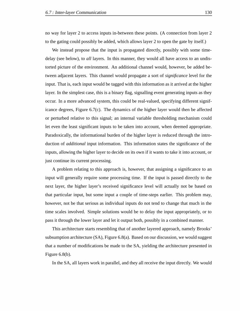
6.7 : Inter-layer Communication 130
no way for layer 2 to access inputs in-between these points. (A connection from layer 2
to the gating could possibly be added, which allows layer 2 to open the gate by itself.)
We instead propose that the input is propagated directly, possibly with some time-
delay (see below), toall layers. In this manner, they would all have access to an undis-
torted picture of the environment. An additional channel would, however, be added be-
tween adjacent layers. This channel would propagate a sort ofsignificancelevel for the
input. That is, each input would be tagged with this information as it arrived at the higher
layer. In the simplest case, this is a binary flag, signalling event generating inputs as they
occur. In a more advanced system, this could be real-valued, specifying different signif-
icance degrees, Figure 6.7(c). The dynamics of the higher layer would then be affected
or perturbed relative to this signal; an internal variable thresholding mechanism could
let even the least significant inputs to be taken into account, when deemed appropriate.
Paradoxically, the informational burden of the higher layer is reduced through the intro-
duction ofadditional input information. This information states the significance of the
inputs, allowing the higher layer to decide on its own if it wants to take it into account, or
just continue its current processing.
A problem relating to this approach is, however, that assigning a significance to an
input will generally require some processing time. If the input is passed directly to the
next layer, the higher layer’s received significance level will actually not be based on
that particular input, but some input a couple of time-steps earlier. This problem may,
however, not be that serious as individual inputs do not tend to change that much in the
time scales involved. Simple solutions would be to delay the input appropriately, or to
pass it through the lower layer and let it output both, possibly in a combined manner.
This architecture starts resembling that of another layered approach, namely Brooks’
subsumption architecture (SA), Figure 6.8(a). Based on our discussion, we would suggest
that a number of modifications be made to the SA, yielding the architecture presented in
Figure 6.8(b).
In the SA, all layers work in parallel, and they all receive the input directly. We would

6.7 : Inter-layer Communication 131
Behaviour 3
Behaviour 2
Behaviour 1
Subsumption
Sensation stream Action stream
Subsumption
(a)
0.0 − 1.0
0.0 − 1.0
Modulation
Modulation
Sensation stream Action stream
Significance
Significance
Layer 1
Layer 2
Layer 3
(b)
Figure 6.8: Brooks’ original subsumption architecture (a), and oursuggestions for extensions and modifications (b).
suggest the addition of communication channels between adjacent layers, where a signif-
icance level can be propagated. (The SA does include the possibility of adding channels
between layers as well.) In this manner, higher layers would naturally have access to more
and more useful representations, through the filtering of the lower layers. In the original
SA, there is no explicit reason for why higher layers should be considered as to working
on more ‘abstract’ or reduced information. Further, we suggest that several behaviours be
implemented inside one and the same layer, i.e. the distribution should not be based on
behaviours but rather on time-scales. Instead of just subsuming (overriding) the output of
lower layers, the output of higher layers could affect or modulate the mapping of the lower
layer. In this manner, very strong innate—and thereby probably important—reflexes can
still operate even if the higher layer is expressing an opposing command. The goal of

6.8 : Discussion 132
learning should be to automatise tasks on lower layers, thereby allowing more uninter-
rupted processing time for higher layers. Or, in the words of Stafford Beer in modelling
the human nervous system:
Now the cerebral cortex, or the board of the firm, or the cabinet of the gov-
ernment, is busy thinking. Therefore it does not wish to be disturbed. There-
fore not too much information needs to flow up the vertical axis to engulf it.
(Beer 1981, page 140).
That is, the goal should be to minimise significance signals, but still maintain system
integrity. The use of a modulating controller, rather than a top-down specifying controller,
means that small and quick adjustments can be done to keep inputs stable, thereby avoid-
ing spurious events to be generated. That is, the robot could turn slightly as wall readings
start to increase, without necessarily creating aneventto achieve such an adjustment.
Note that there is no principled reason for why a task could not be learnt on a low
layer rather than on a higher layer. The only difference between layers is the time laps
between (high) significance signals. (The lowest layer has a constant high significance
signal, or a significance signal related to the amount of change which occurs between two
successive samplings.) Higher layers do have the advantage of only being notified when
inputs relating directly to the task are received, whereas the lower layers need to process
many—for the task irrelevant—inputs.
6.8 Discussion
We have presented a general design for layered control systems capable of learning de-
layed response tasks with arbitrarily long delays. The approach is based on extracting
events from the input stream and then reacting to these events through top-down control.
Different alternatives in implementing the control system were presented, namely reac-
tive, specifying and modulating controllers. Of these, the modulating controller seems to
be most promising, allowing both top-down information and direct sensory inputs to be

6.8 : Discussion 133
taken into account. Using a modulating controller, the system can also affect the input-
to-output mapping as to focus attention to particular sub-sets of the sensory array.
Further, different representational issues were discussed when it comes to representing
events. Two major problems were discussed, namely that of binary, localistic, expert rep-
resentations’ orthogonality and that of constructive systems having growing back-ends.
While using a prototype class representation would resolve both these issues, we would
suggest that there really is no need to propagate the actual prototype but instead just a
signal that something interesting has occurred. This signal could work essentially like a
gating signal, letting only significant inputs reach the higher layers of the system. How-
ever, we point out that this would put the higher layers at the mercy of the lower layers’
gating systems and suggest something more in line with that used in the subsumption
architecture, namely that all layers receive all the input all the time. The difference be-
ing that higher layers also receive information about the inputs’ significance, from lower
layers, thereby avoiding processing inputs which are not relevant for the task. Only when
important information is received, is the higher processing interrupted. The robot’s higher
layers can thus find time to do some higher-level processing and laying out of plans for
the future, or even do some well-deserved resting when things are under control at the
lower layers.

Chapter 7
Learning on Reduced Sensory Flows
�E HERE DIRECTa mobile Khepera robot to learn a delayed response task. The
task involves finding the relevant indicators for making a context-dependent
choice at a substantially later point in time. More specifically, the robot needs to learn
that the lights (rather than actual road signs) it passed by at an earlier point in time,
indicate the correct way to turn at a later upcoming junction. Two different learning
techniques are first presented: a simple instantaneous feedback (supervised) learner and a
more complex, but also more realistic, delayed reinforcement learner. The inputs to these
learners are provided as localistically encoded events, and the relevance of these events
needs to be deduced and coupled to output behaviours, here also localistically encoded.
The coupling needs to be context-dependent, i.e. a number of past events need to be taken
into account when deciding what behaviour to select. In both experiments, the same set of
pre-defined behaviours is used. The behaviours (input-to-output mappings) are realised
through simple handwritten programs, which base their outputs on the immediate sensor
readings. Each behaviour makes use of only a subset of the available sensory array; they
only focus on the sensors which are really necessary for their functioning. Both learners
come to master the task without much difficulty, regardless of the delay periods involved
between the lights and the junction. A more difficult scenario, where distracting events
occur during the delay period is also introduced and discussed. We then—using a third
learner—look at how the system can construct behaviours on its own, through a quite
134
7.1 : Setup 135
massive trial-and-error process1.
7.1 Setup
A simulated version of the Khepera robot was used in both experiments. The activation
of the eight distance sensors, the two motors, and two of the robot’s light sensors, placed
in concert with distance sensors 1 and 6 in Figure 7.2(a), were normalised to the range
� � �� � and fed as input to the architecture. That is, the event extractor (an ARAVQ)
received a total of 12 inputs. The parameter settings of the ARAVQ wereÆ � ��,
� � ��, � � and� � � �. This led to the extraction of eight different experts
for the constructed T-maze environments shown in Figures 7.1 and 7.5. The setting of
these parameters affects the number of experts extracted by the ARAVQ and, hence, the
rate of switching between these experts.
The parameters were chosen to get a sufficient set of events for solving the task;
at least the stimuli and cue for response must trigger events or learning is practically
impossible. A robot which has only a single event type, will never be able to learn any
useful associations on the event level. It is worth noting that having ‘too many’ events
do not seem to be as severe as having too few. In the worst case, we trigger an event for
each an every input, but then we are effectively back on a time-step based representation
like we started with in the first place. (Albeit the representations may now be distorted
through the extractor’s mapping to the event space.) We would therefore recommend that
parameters generally be set to promote the incorporation of a large set of events rather
than using an overly restrictive setting.
The event extraction discarded the repetitions of each expert, leaving sequences which
are only six characters long. A character was manually assigned to each of the eight
extracted experts, for presentational purposes only. An interpretation of each expert is
shown in Table 7.1, based on how the ARAVQ seems to apply the experts. The! and�
1Most of this chapter has been published in Lin˚aker & Jacobsson (2001a), Bakker, Lin˚aker & Schmid-huber (2002), and Bergfeldt & Lin˚aker (2002).

7.1 : Setup 136
20
d24
a
a
a
b61
113
f87 27
a
d24
a
a19
60
114
25 85
c
e
(a) (b)
Figure 7.1: Different cases for the delayed response task and theresulting input classification at each location along thesimulated robot’s path where each expert was allocated aseparate shade, here plotted as a trail behind the robot. Thesubscripts denote the number of repetitions of each expert.
experts were only extracted for the Extended Road Sign Problem, which we present later
in the chapter.
Table 7.1: The eight automatically extracted experts and how they canbe interpreted.
expert interpretation
� corridor� corridor + left light� corridor + right light� junction� wall on left side only� wall on right side only! left-turning corner� right-turning corner

7.2 : Behaviours 137
The time-stepped real-valued input stream was thus reduced through the event extrac-
tion to an asynchronous eight-pattern binary stream. This stream was now to be used for
controlling the robot; it would need the capability of turning left or right at the junction,
as well as the basic capability of staying on the road (in the corridors). For this, three
basic behaviours were constructed manually.
7.2 Behaviours
Three different input-to-output mappings, or behaviours, were constructed: a corridor
follower, a left wall follower, and a right wall follower, presented in Figure 7.2. We
use a modulating controller, thus the top-down modulation can focus the ‘attention’ on
a particular sensory subset. Here, the focus is set completely on only two of the ten
available inputs (eight distance sensors and two proprioceptive motor sensors). To follow
the right wall, for example, only requires the robot to take the right and front-right sensors
into account, the others being relatively unessential for the task2.
For presentational purposes, we assign a character to each of these three behaviours,
creating the three-symbol ’output alphabet’ shown in Table 7.2.
7.3 Learner I: Immediate Feedback
In this setup, a feedback signal was provided for each event to behaviour mapping, indi-
cating its appropriateness. (This feedback was manually constructed based on the event
interpretations we listed in the previous sections.) Any type of basic learner which is
able to take temporal ordering into account should be able to learn this mapping, as it has
become trivial (the data set is in Section 7.3.1). We chose a Simple Recurrent Network
(SRN) learner, to show that this system no longer would have any problems learning the
2The Khepera robot has eight infrared proximity sensors with integer activation in the range��� �����,� denoting no object present within sensor range and���� denoting an obstacle very close. The robot hastwo separately controlled wheels which can be set to integer values in the range����� ���, ��� denotingmaximum backward spinning,� no wheel movement, up to�� which rotates the wheel forward at maximumspeed.

7.3 : Learner I: Immediate Feedback 138
left motor right motor
1
23 4
5
6
78
} else { motor[LEFT] = 5; motor[RIGHT] = 5;
}
motor[LEFT] = 5; motor[RIGHT] = 0;
motor[LEFT] = 0; motor[RIGHT] = 5;
/* Corridor follower */if (sensor[5] > 800) {
} else if (sensor[2] > 800) {
(a) (b)
motor[LEFT] = 5; motor[RIGHT] = −4;
motor[LEFT] = 2; motor[RIGHT] = 5;} else { motor[LEFT] = 5; motor[RIGHT] = 5;}
/* Left wall follower */if (sensor[2] > 200) {
} else if (sensor[1] < 800) {
} else { motor[LEFT] = 5; motor[RIGHT] = 5;
}
motor[LEFT] = −4; motor[RIGHT] = 5;
motor[LEFT] = 5; motor[RIGHT] = 2;
/* Right wall follower */if (sensor[5] > 200) {
} else if (sensor[6] < 800) {
(c) (d)
Figure 7.2: The Khepera robot and the three hand crafted behaviours.
Table 7.2: The three hand crafted behaviours.
behaviour description
" corridor following# left side wall following$ right side wall following
task; this learner could not handle the task at the time-step level, as we discussed in the
previous chapter. The SRN also has the property of mapping its inputs to an internal
representation based on their functional values; this provides an excellent base for event
filtering, i.e. the removal of irrelevant or distracting events from the event stream.

7.3 : Learner I: Immediate Feedback 139
7.3.1 Input and Output Strings
As the continuous-valued input and output streams both had been discretised, the system
had two essentially symbolic streams to work with. The (input) event stream had a total
of eight differing patterns, while the (output) behaviour had a total of only three differing
patterns. The problem was thus reduced to the level of learning to correlate eight-symbol
input strings with three-symbol output strings, of length six, as depicted in Table 7.3.
Table 7.3: The extracted sequences of expert winners and thebehaviours that should be selected for the paths taken inFigure 7.1.
case sequence
Left turn� � � � � �" " " # " "
case sequence
Right turn� � � � � �" " " $ " "
7.3.2 The Simple Recurrent Network
The simple recurrent network (SRN) (Elman 1990) is essentially a three-layer feed-
forward network which stores a copy of the previous hidden activation pattern and feeds it
as additional input at the next time-step (see Figure 7.3). This provides a memory trace of
previous inputs which enables the network to learn associations over several time-steps.
The output of the SRN (for an arbitrary number of nodes) is defined as:
���� � ����
������� � ��� (7.1)

7.3 : Learner I: Immediate Feedback 140
copy 1:1
ARAVQ winner: i(t)
behaviour: o(t)
hidden: h(t)
context: h(t−1)
Figure 7.3: The SRN. The previous hidden node activation is part ofthe input to the hidden nodes at the next time-step.
where the hidden activation is defined as
����� � ����
�������� ���
�������� �� � ���� (7.2)
and���� is the input at time�. The index is used for identifying the output nodes,%
and are used for the hidden nodes (at time� and� � � respectively), and� is used for
the input. Biases are introduced as additional elements in the weight matrices,� and�
(indexed with�). The function,� , is the sigmoid activation function���� � ����� ����.
Since� is differentiable, the network can be trained using gradient descent.
The SRN was to specify which of the three behaviours (Section 7.2) the robot was
to employ until the next event occurred. A simple localistic coding scheme was used
for the input events as well as the behaviours, that they could be used with the SRN. As
two hidden nodes were used, an 8-input, 2-hidden, 3-output SRN was created. Network
weights were randomly initialised in the interval��� � �� �, the learning rate was 0.01
and a momentum of 0.8 was used. The training set was the two extracted sequences, for

7.3 : Learner I: Immediate Feedback 141
the left and right turn, respectively, as shown in Table 7.3. The network was trained for
� epochs using a version of back-propagation through time (BPTT) whichunfolded
the recurrent connections of the network. The BPTT here unfolded the network 5 times
according to the scheme presented by Werbos (1990).
7.3.3 Architecture
In addition to the three hand crafted behaviours, a simple selection mechanism was im-
plemented. At each time-step, it detected the most active output node of the SRN and
executed the code (Figure 7.2) associated with the behaviour. The architecture is sum-
marised in Figure 7.4.
Unsupervisedclassification(ARAVQ)
winnertake all
winnertake all
Sensation Action
Response (SRN)
(hand−crafted)
Event classes Behaviours
Response (hand crafted)
Modulation
Event based
Time−step based
Figure 7.4: An event-based controller with two layers. The bottomlayer works on time-stepped Level 1 representations, whilethe top layer works on event based Level 3 representations.
7.3.4 Results
As expected, the SRN had no problems learning the correct associations between the light
stimuli � and� and the behaviours# and$ occurring two events later. That is, the system
could turn in the right directionirrespective of the length of the delayas this temporal

7.4 : The Extended Road Sign Problem 142
information was removed in the event extraction. The Road Sign Problem could thus be
solved using a straight-forward gradient descent method.
However, if more events were extracted, as a result of a different setting of ARAVQ
parameters, the problem would be more difficult to learn as a result of more intervening
events. This effect could also arise as a result of degrading or noisy inputs, causing the
ARAVQ to trigger more events. A situation where intermediate events are a result of
the physical environment would result in similar difficulties. Thus, we have a problem
similar to that of Rylatt and Czarnecki, but on the level of intermediateeventsinstead of
intermediate time-steps. We call this problem ‘The Extended Road Sign Problem’.
7.4 The Extended Road Sign Problem
While the length of the delay between the stimulus and the response has become irrele-
vant through the use of event extraction, the system would still have problems handling
distracting events during the delay. That is, if the input changes drastically during the
delay, intermediate events will be generated. This means that the problem of finding rela-
tionships between the stimulus and the subsequent response will become harder as there
are a number of intermediate distracting events. Examples of this are shown in Figure 7.5
where there is a right or left turn in the corridor after the stimulus has been passed, gener-
ating another three events which, however, are of no relevance for the task, i.e. they serve
only as distractions.
The SRN still managed to find the correct association, but only if it was first trained
on the simpler tasks, and then continued training on the more difficult examples shown in
Figure 7.5. This is a well-tried method of solving these types of problems where the task
is too difficult to learn directly. Such training on incrementally difficult problems, starting
with an easier version of the problem, is known to help the learning process significantly
as shown by Elman (1993). The hidden node activation plot of an SRN which has learnt
the task is depicted in Figure 7.6. Note that a number of clusters have formed for each of
the functional states the robot can be in.

7.4 : The Extended Road Sign Problem 143
ab f10 63 44 14
f 21
a
a
218
d
a85
g
f
26
22
26
a
e
he13 a a
d
a95
c 10664223
22
221
26
22e
(a) (b)
Figure 7.5: Two examples of distracting events (turns) happening inbetween the stimulus (light) and the cue (junction).
0 0.1 0.2 0.3 0.4 0.5 0.6 0.7 0.8 0.9 1
0
0.1
0.2
0.3
0.4
0.5
0.6
0.7
0.8
0.9
1
Hidden node 1
Hid
de
n n
od
e 2
Goal undefined
Goal to the left
Goal to the right
Follow right wall
Follow left wallfollowing
Right wallfollowing
Left wall
Corridor following
Figure 7.6: Hidden node activation of the SRN.
When irrelevant inputs, such as corners (input characters! and�), are received by the
SRN, the state remains relatively stable, i.e. it stays in the same location as the previous

7.4 : The Extended Road Sign Problem 144
time-step. That is, large movements in the internal (hidden node) activation space occur
only whenfunctionally importantevents occur. When, for instance, input character� (left
stimulus) is received, the activation jumps to the upper right corner of Figure 7.6 and
stays there until the input character� (the cue for responding) arrives. At that time, the
activation quickly jumps to the upper left corner, making the robot activate its left wall
following behaviour, effectively starting to turn left at the junction. A similar situation
occurs if instead the other stimulus is present, where the bottom right and left corners
are used by the SRN. (Before either stimuli has been encountered, the SRN state is in
the upper right corner, i.e. this particular robot has a bias for turning left at junctions.)
Since spurious events do not affect the internal state of the SRN in a way that disturbs
its performance, the system should exhibit graceful degradation if the ARAVQ is fed
deteriorating data (slightly noisy data will be filtered by the ARAVQ and thus not affect
the SRN at all).
We can now also sketch a solution to the Extended Road Sign Problem. If the hid-
den activation space of this SRN was clustered, using for example another ARAVQ, the
functionally unimportant events would likely cause repetitions of the same expert as they
would lead to only small perturbations in the state space. Only when functionally impor-
tant events occur, such as the stimulus or cue, do large jumps in activation space occur,
thereby leading to another expert perhaps becoming the best match. Then using the same
filtering process used for repetitions of input patterns, the irrelevant events would be re-
moved. Note that this solution is based on a Level 3 system (SRN) which has already
successfully learnt the associations in a relatively simple scenario. The filtering can then
extract information which effectively lets the next higher level (Level 4) handle delays
with an arbitrary number of distracting events as they will be filtered out in the afore-
mentioned process.

7.5 : Learner II: Delayed Reinforcement 145
7.5 Learner II: Delayed Reinforcement
A more realistic learning scenario is one in which feedback is not provided directly after
each event. Instead, the robot is allowed to move about in the T-maze for some time,
without any feedback relating to theinternal event and behaviour mapping processes. If
it ends up in the correct goal zone—anexternallyobservable occurrence—it receives a
positive reinforcement signal, otherwise it receives a negative signal. The system then
has to assign this credit to its previous interaction, portioning it out among the internally
applied mappings3.
7.5.1 Architecture
In this work, the reinforcement learning system was based on a Long Short-Term Memory
(LSTM) recurrent neural network (Hochreiter & Schmidhuber 1997), which has been
shown (Bakker 2002) to be very good at learning temporal dependencies. Again, the
ARAVQ was set to extract events from the incoming sensory flow (see Section 7.1), and
the same three behaviours were used as in the previous experiment (see Section 7.2). The
events were sent to a Reinforcement Learning LSTM (RL-LSTM) network, which kept
a trace of previous events and which through its learning mechanisms could assign the
received credit to the relevant indicators. An overview of the architecture is presented in
Figure 7.7.
The RL-LSTM had to learn the coupling between the (input) events and the (output)
behaviours. Once the goal position was reached, it would receive a scalar reward � �.
If the goal was not reached, it would instead get a scalar reward of � � ��. Details of
the RL-LSTM can be found in Bakker et al. (2002). The position of the light (and thus
the correct turning direction) was randomly assigned for each episode; there was no fixed
ordering between the two cases.
3We have published this work in Bakker et al. (2002); the contribution here was the ARAVQ prepro-cessing of the inputs, not so much on the reinforcement learning scheme, which was the work of Bakker.

7.5 : Learner II: Delayed Reinforcement 146
RL-LSTMnetwork
L: left wall follower
R: right wall follower
F: corridor follower
ARAVQ event extraction
sensorydata
concepts actionsL, F, R
motorcommands
HIGHLEVEL
LOWLEVEL
ENVIRONMENT
reward
Figure 7.7: A delayed reinforcement learner which can learn complextemporal relationships.
7.5.2 Results
The RL-LSTM had no problems learning that the lights (road signs) were the relevant
indicators for the task. It quickly learnt that going forward in the junction was not a
very good alternative; it would never lead to a positive reinforcement. Going left or right
instead became the applied behaviours, and after about� training episodes (T-maze
runs), Figure 7.8, the correct contexts for using these behaviours had been sorted out.
The RL-LSTM would never reach a� � correctness as it employed an exploration
mechanism.
The Extended Road Sign Problem (Section 7.4) was also tested for the RL-LSTM
architecture. A more complex maze was constructed which contained a number of dis-
tracting events along the way, Figure 7.9(a). As with the standard Road Sign Problem,
positive reinforcement was only given for actually reaching the goal position. As ex-
pected, learning that the light was the correct indicator for the final decision, required
many more training episodes than previously. The RL-LSTM eventually had assigned
the credit were it was due; after about� episodes the correct associations had been
learnt, Figure 7.9(b).

7.5 : Learner II: Delayed Reinforcement 147
0 1000 2000 3000 4000 50000.4
0.5
0.6
0.7
0.8
0.9
1
Number of episodes
Pro
b. o
f rea
chin
g go
alFigure 7.8: Learning curve for the RL-LSTM architecture, showing
the probability of reaching the goal location in the RoadSign Problem.
G
S
G
0 1 2 3 4 5 6x 10
4
0.2
0.4
0.6
0.8
1
Number of episodes
Pro
b. o
f rea
chin
g go
al
(a) (b)
Figure 7.9: A more complex maze (a) where the robot needs tonegotiate a number of junctions (distractions) beforereaching the junction (the cue) which requires it to use thetrace of the light position. The learning now takes longer(b), but the relevant indicator is still identified.
The activation for two different episodes of the memory cells (internal nodes)�� of the
RL-LSTM—three were used—are depicted in Figure 7.10. The first ten events reflect an
episode where the goal was to the left; memory cell�� sustained a high activation once

7.6 : Learner III: Evolution 148
the indicator stimuli was passed. Then another episode begins, where the goal instead is
placed to the right, and memory cell�� now has a different activation trace, enabling the
system to use it as an indicator for how it should behave when the cue (the junction) is
encountered. Memory cells�� and��, on the other hand, have the same traces for both
episodes; they do seemingly not encode any useful information.
0 5 10 15 20−6
−4
−2
0
2
4
6
8
10
12
Events
Val
ue
c 1 c 2 c 3 reward
Figure 7.10: Activation of the three RL-LSTM memory cells for twosucceeding episodes, as well as the reward signal.
7.6 Learner III: Evolution
In the previous learners, three behaviours (input-to-output mappings) were manually con-
structed and used: a corridor follower, a left-wall follower and a right-wall follower. One
such behaviour was active for a number of time-steps, until a new event was triggered, at
which time another behaviour could be selected. Each behaviour was realised through a
small procedural program which produced a motor output based on the current time-step’s
input. Each behaviour-program operated on only a select sub-set of sensors, deemed rel-
evant for that specific task. Instead of this all-or-nothing regime, the focus should ideally
be controlled with finer granularity, weighing some sensors just slightly more or less than
the others. Further, the input-to-output mapping should take greater advantage of the

7.6 : Learner III: Evolution 149
available output space. The aforementioned controllers only utilised seven different mo-
tor settings in total, i.e. the controllers took advantage of less than two percent of the
output space. (Each of the two motors could be set to an integer in the range [-10,+10].)
To allow the controller access to a larger part of this space, not just by adding some ran-
dom ‘noise’ to the output values, the action can be made directly dependent, linearly or
non-linearly, on the specific sensation at each time point. This should enable the system
to quickly make small, smooth, adjustments in its interaction. Neural networks seem to
be obvious candidates for implementing the controller, with behaviour top-down modula-
tion working through sigma-pi connections or second order weights, an approach similar
to Ziemke (1999), thereby allowing behaviour node activations to affect the lower-level
mapping continuously. This is investigated in the following.
7.6.1 Related Work
The approach of viewing behaviours as continuous input-to-output mappings (vector
fields) corresponds to the theory of Hybrid Control Loops, see e.g., Davoren et al. (2002)
for an introduction. The similarity lays in theswitched plantswhich are control systems,
consisting of a finite number of vector fields (behaviours). The control input to a switched
plant is via discrete input events which select which vector field is to be active; the system
switches between the vector fields. Such systems are, however, designed to work in some
pre-defined operating limits, i.e. an unsupervised clustering of the input or exploration of
different vector field configurations (input-to-output mappings) does not take place.
Here, we show that a system can form its own behaviours as a side-effect of learning
the task. Interestingly, we now find solutions which are quite unexpected but perform
almost perfectly. In fact, the simple 2-choice (left/right) delayed response task outlined in
the previous chapter—the Road Sign Problem—is now solved without using any internal
state, i.e. in a purely reactive manner! But when the task is made more difficult, like a
3-choice task, the solutions switch to instead being based on keeping an internal trace of
the encountered light activation, as might be expected.

7.6 : Learner III: Evolution 150
Layer 1
Layer 2
gating
modulationARAVQ
Figure 7.11: System implementation. Sensor readings arecontinuously fed through a simple feed-forward networkand quickly produce a set of motor activations. AnARAVQ classifies inputs and triggers events onclassification shifts, updating Layer 2 which specifies aset of modulatory values of the lower mapping, assumingthat the gating node has been activated, otherwise nomodulation is applied.
7.6.2 Architecture
An important issue in realising behaviours as neural network input-to-output mappings is
the manner in which the higher layer enforces its behaviours on the lower layer. There are
several different approaches available for suchmodulationof a neural network. Layer 1 is
expected to produce simple reactive behaviours like obstacle-avoidance, which are valid
throughout the execution of all the tasks dealt with here. That is, Layer 1 should never
be entirely subsumed by the higher layers, it should only be modified to a limited degree.
An overview of the architecture is presented in Figure 7.11.
Layer 1 produces its behaviour through a simple input-to-output neural network-style
mapping which is determined by a set of connection weights. These weights can be
modified to achieve different behaviour. There are at least three choices for modifying

7.6 : Learner III: Evolution 151
the Layer 1 weights with modulation coming from higher layers: the weights can be
completelyreplacedwith a new set, the weights can bemultipliedwith a set of values, or
finally, a set of values can beaddedto the weights.
7.6.3 Top-Down Modulation
A subsuming approach would (temporarily) replace the weights with new values, thereby
completely overriding the old ones (Pollack 1991, Ziemke 1999). That means that no
information is ”inherited” into the new mapping. That is, the new values not only need
to reflect the new behaviour-producing values but also all the old, existing, values in the
mapping that might be needed for the correct functioning of the system. This is a wasteful
approach since it requires massive redundancy in the coding of the different behaviours.
The existing Layer 1 values can instead simply be multiplied with new values, increas-
ing or decreasing the values ever so much to achieve a qualitatively different interaction
with the environment. The same holds if addition is used as a modulatory realisation.
These approaches both use the existing information, contained in the Layer 1 weights.
Addition does have some advantages over the multiplicative approach. For instance, if
Layer 2 is damaged, no longer producing any output, an addition of nil/zero does not
affect Layer 1 at all. A multiplication of nil/zero, however, cancel out all the weights,
rendering the entire system irresponsive. (If the system is to be constructed bottom-up,
with layers being added at different times, an additive approach would therefore also be
more appropriate.) Further, if the weight we are about to modulate has a value very close
to zero, multiplication will not affect the mapping considerably, whereas addition would
work regardless.
Primarily due to the advantages when dealing with near-zero weights, we here inves-
tigate the additive approach. The output activation of Layer 2 is thus added to the weights
of Layer 1, and are kept constant at these new values until the next event generates an up-
date to Layer 2. However, instead of modulating all the weights of Layer 1, only the bias
weights of the output nodes are modified. The bias weights can be considered as speci-
fying a kind of innate threshold or firing propensity of the nodes. An extension would be

7.6 : Learner III: Evolution 152
to modulate all the weights, thereby the system would be able to focus on specific sub-
sets of the sensory array at different points in time, which may be of great value in some
situations. However, such an approach would also lead to a drastically larger weight con-
figuration search-space. As discussed in the succeeding sections, the modulation of only
the bias weights turns out to be sufficient for the tasks dealt with here.
7.6.4 Behaviour Gating
Initial experiments indicated that the system had a hard time learning the Road Sign Prob-
lem as every Layer 2 update led to new internal activation patterns and thus also new out-
put activations. These activations affect the Layer 1 functioning and it is very difficult for
Layer 2 to only produce internal states which only lead to notable activations on the out-
put nodes at the time of the junction and not everywhere. Therefore, a simplegating node
was added which only propagates the modulation when it is active, similar to a decision
unit used in Ziemke (1999) and Ziemke & Thieme (in press). In this manner, theinternal
state of Layer 2 does not always affect the Layer 1 mapping, but only at the specific points
in time where the gating node is active. The system is given full control over its gating
node (its incoming weights), i.e. it can choose to set it active all the time, or perpetually
inactive. This leads to some interesting solutions, as discussed in the following.
It is worth pointing out that the basic idea of Layer 2 is closely related to memory
cells (Hochreiter & Schmidhuber 1997), where the use of two gate units, encapsulates
the state to circumvent the problems mentioned here with the continuous activation flow
coming from Layer 2. The event extractor filters out unwanted, repeated sensor activa-
tions coming from Layer 1. This event extractor thus acts as an input gate to Layer 2.
Further, Layer 2 has the ability to not affect Layer 1 at all times by using the gating node,
which can be seen as an output gate.

7.6 : Learner III: Evolution 153
7.6.5 Experiments
In these experiments, the Khepera simulator YAKS (Carlsson & Ziemke 2001) was used
to produce behaviours from an unsupervised exploration for the 2-choice Road Sign Prob-
lem4. All eight distance sensors, and the two light sensors pointing straight to the left and
right (numbers 1 and 6) were used, i.e. the system had a total of ten inputs. In Layer 1, this
meant that ten input nodes were directly connected to two output nodes which specified
the motor activation values. Linear activation functions were used on all output nodes on
each layer, and a step-function (0 if net input smaller than 0.5, otherwise 1) on all internal
nodes.
The network was trained using a simple evolutionary algorithm. There was therefore
no need to have differentiable activation functions, as back-propagation was not applied,
and using binary internal activation lent itself to easy analysis through the extraction of
Finite State Automata (see next section) once training had completed. Weights in the net-
work were bounded to the interval -10.0 through +10.0, and were modified by a Gaussian
mutation operator with a variance of 0.5. (No crossover operator was used.)
The ARAVQ was set to classify the inputs based on a dynamic set of experts. The
ARAVQ’s four parameters were set as follows: novelty criterionÆ � ��, stability cri-
terion � � ��, buffer size � � and learning rate� � � �. An event was generated
only when the ARAVQ assigned an input into another expert than the previous input,
thereby providing a sort of temporal filtering. Then the prototype (model vector) for the
new winning expert was fed as input into Layer 2, thereby providing a spatial filtering on
the signal. Upon such an update, activation was propagated through the connections to
finally specify an activation pattern on the two output nodes on Layer 2.
A simple T-maze was created and the robot was placed in the lower part of the maze,
facing the direction of the junction. A small amount of noise (���) was added to the
starting coordinates and starting direction. The robot was then free to move and might
4The Khepera simulator (Michel 1996) used in the previous chapters was not used here as larger worldsand better incorporation of evolutionary search methods were deemed necessary.
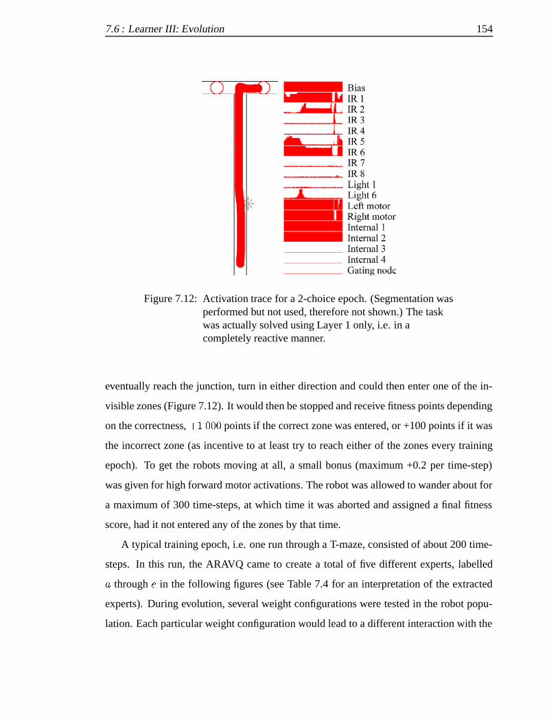
7.6 : Learner III: Evolution 154
Figure 7.12: Activation trace for a 2-choice epoch. (Segmentation wasperformed but not used, therefore not shown.) The taskwas actually solved using Layer 1 only, i.e. in acompletely reactive manner.
eventually reach the junction, turn in either direction and could then enter one of the in-
visible zones (Figure 7.12). It would then be stopped and receive fitness points depending
on the correctness,�� points if the correct zone was entered, or +100 points if it was
the incorrect zone (as incentive to at least try to reach either of the zones every training
epoch). To get the robots moving at all, a small bonus (maximum +0.2 per time-step)
was given for high forward motor activations. The robot was allowed to wander about for
a maximum of 300 time-steps, at which time it was aborted and assigned a final fitness
score, had it not entered any of the zones by that time.
A typical training epoch, i.e. one run through a T-maze, consisted of about 200 time-
steps. In this run, the ARAVQ came to create a total of five different experts, labelled
� through� in the following figures (see Table 7.4 for an interpretation of the extracted
experts). During evolution, several weight configurations were tested in the robot popu-
lation. Each particular weight configuration would lead to a different interaction with the

7.6 : Learner III: Evolution 155
environment, which in turn would produce different numbers of experts. For example, a
robot which just stands still each time-step would just extract a single expert for its static
input, whether ones with very erratic behaviour could extract a much larger number of
experts due to the resulting richer sensory experience.
7.6.6 Results
First, experiments were conducted on the 2-choice (left/right) delayed response task. Sur-
prisingly, solutions were frequently discovered where the gating node was inactive during
the entire epoch, yet the robot turned correctly at the junction. Analysis of this solution
showed that the robot controller did indeed handle the task using only the simple reactive
Layer 1 network. When passing the light on either side, the reactive mapping led to the
robot moving closer to the opposite wall. Thereby it would receive a higher activation on
the side sensors on one side in the succeeding time-step. Instead of keeping an internal
trace of the light activation, it used its interaction with the environment as a sort ofscaf-
folding. Performance on the task using this approach was nearly perfect, i.e. a quite valid
solution, although Layer 2 did not show its use the way expected.
A more difficult task was then introduced, namely a 3-choice task. The inputs were
again classified by the ARAVQ and when the input started to change, causing a different
classification, an event was generated. The input stream was thus segmented based on the
events (Figure 7.13). As earlier, a light on either the left or right side would imply a turn
in the respective direction. Now, however, the robot could encounter two lights, one on
each side simultaneously, indicating that the robot should continue straight forward at the
junction.
Solutions to the 3-choice task did make full use of Layer 2. Interestingly, the light
trace was now kept completely internally, i.e. the robot did no longer rely on using its
world as scaffolding. This is likely due to the following: When a ”double light” was
passed, the robot could lose sight of one of the lights a little sooner than the other, thereby
receiving the input corresponding to asinglelight stimulus. It could therefore no longer
rely on individual inputs as providing the correct stimulus, but needed to take more inputs

7.6 : Learner III: Evolution 156
Figure 7.13: Activation trace for a 3-choice epoch, showing thesegmentation of sensory data. Each expert, here labelled� through�, is depicted in a different colour. The gatingnode was here used appropriately and the task was solvedby internally keeping track of the passed light stimuli.
into account by storing them internally.
The use of the gating node was quite elegant. When left and right wall sensors started
to drop, thus generating an event at the junction, the gate node was activated. Once the
junction had been negotiated, side sensors were reactivated, causing another event and
thereby deactivating the gating node until the next junction (Figure 7.13).
The modulation increased the motor bias weight on the appropriate side (Figure 7.14),
thereby causing the robot to turn in the desired direction. By slightly nudging the firing
propensities in some direction, a qualitatively different behaviour of the entire system was
thus generated.
To analyse how the internal nodes were used, Finite State Automata (FSA) were ex-
tracted for Layer 2. As different numbers of internal nodes were tried, several FSA were
extracted, for solutions which utilised different numbers of internal states. Only the vis-
ited states are presented in the figures. For readability we use the abbreviations C, LL, J,
RL and DL (Table 7.4) instead of� through�, in the FSA.

7.6 : Learner III: Evolution 157
(a)
(b)
(c)
(d)
Figure 7.14: Hinton diagrams showing the un-modulated weights (a)and the modulated weights during forward motionthrough the junction (b), while turning left (c) and turningright (d) in the junction. Modulation only took place onthe bias weights. Positive weights are illustrated withbright colour rectangles and negative with dark ones. Thesizes are directly proportional to weight magnitudes.
Table 7.4: Extracted model vectors and an interpretation.
model vector interpretation abbreviation
� Corridor C� Left light LL� Junction J� Right light RL� Double light DL

7.6 : Learner III: Evolution 158
For example, the epoch depicted in Figure 7.13 involves a controller based on four in-
ternal nodes. This corresponds to the FSA in Figure 7.15(c). The initial internal activation
in this epoch is 0010. When the event� (LL) is triggered, the internal activation pattern
switches to 0000. Then event� (C) is triggered, returning the activation to 0010. When
the junction is encountered, event� (J) is triggered and the pattern changes to 0001 and
the gate is activated, actively modulating the Layer 1 mapping so that the robot turns left.
Finally, when the junction has been passed, an� event (C) is triggered and the activation
pattern returns to 0010, and the gate is deactivated. The robot is now prepared for another
set of lights as it continues down the corridor.
In all solutions, the gating node was activated at the junction event, and in-activated
at all others. As the gating node was always activated at the junction, irrespective of the
turning direction, and as the systems were able to handle the 3-choice task, this implies
that at least three different modulation patterns were used. That is, for these solutions to
work, there needed to be at least three different states for the internal nodes, which gen-
erated these three different modulation patterns on the output nodes. Such a set of three
states were indeed present in all working solutions, irrespective of the number of internal
nodes, and these states have been marked in a darker shade in Figure 7.15. Consistent
with this, we found no solution based on just a single hidden node, as then only two pos-
sible states exist. (One possible work-around for this would have been to combine the
internal state with scaffolding, similar to the 2-choice solution.)
As can be observed in the extracted FSA in Figure 7.15, the controllers worked slightly
differently. All depicted controllers received an RL event before the DL event. That
is, the robots always detected the right side light slightly in advance of the left when
encountering a double light. However, the two and three hidden node controllers then
always lost sight of both lights simultaneously while the four internal nodes controller
may then perceive only a left side light as it moved on. This is due to differences in
these controllers’ Layer 1 nets, which made the robots turn slightly and slow down when
encountering double lights, resulting in this LL event being generated.

7.6 : Learner III: Evolution 159
forward right turn
left turn
J
Start
CLL
{RL, J}
C
{DL, J}
{LL, C} {RL, C}11
0100
10
(a)
C
forward
{LL, J}
J
Start
left turn
right turn
C C
C
J
DL
RL
LL
RL
111
001
100
101
011
000
C
J J
{C, LL}
C
C
LL
DL
C
RL
C
J
C
forwardleft turn
right turn
Start
C
0100
1010
10010001
1011
11000000
0010
(b) (c)
Figure 7.15: Extracted self-organised FSA for different solutionsusing two up to four internal nodes. The internal states,their coupled behaviour and also the transition signalsthemselves have all been autonomously constructed bythe system. States in darker shade depict states where thesystem has decided that modulation could take placegiven that the gate node was active (i.e. the robot being ina junction). These states have been labelled with theircorresponding observable behavioural consequences.
The networks were not reset in between epochs, therefore any ”clearing” of the in-
ternal activation had to be performed by the networks themselves. The earliest time for
such a resetting of the internal state would be the event being generated just after the
junction had been passed. At that time the light activation trace no longer would be of
value. As training was conducted on a strictly sequential repetition of forward, left-turn,

7.6 : Learner III: Evolution 160
Figure 7.16: Complete run through a maze, dark circles denotinginvisible ”danger zones” which needed to be avoided byturning according to the light stimuli. The system had nodifficulties in navigating the maze appropriately eventhough it had never encountered it before.
then right-turn epochs, it might be expected that the solutions would reflect this particular
configuration of turns. This was, however, not the case, as can be read out of the FSA.
To test the performance of the robot controllers outside the T-maze environment in
which they had been trained, a set of mazes was created. The robot was put in one end
of the maze, and had to find its way trough the maze using guiding lights placed before
each junction. If an incorrect turn was taken the robot could enter a ”danger zone” and
would be destroyed. Figure 7.16 depicts the trajectory of a robot navigating through the
maze without difficulties, avoiding dead-ends and reaching the finish safely. Tests were
also conducted with a random sequence of left/right/forward epochs, and more than���
out of� such epochs were correct.
7.6 : Learner III: Evolution 161
7.6.7 Summary
We have shown how a simple layered system can self-organise into a set of distinct states
and qualitatively different behaviours as a result of learning a robotic delayed response
task. All the system was fed was the noisy sensor readings of the robot as it moved about
in the different environments, receiving a simple reinforcement, or fitness, at interspersed
intervals. From this continuous input signal, the system extracted a set of events in a
bottom-up manner. These events served as triggers for a recurrent neural network which
kept a trace of the passed stimuli (lights) and modified the functioning of the lower level
network when response cues (junctions) were encountered.
The use of an internal gating node proved fruitful and the system learnt to use this in
order to keep the state of Layer 2 internal, i.e. not propagating the modulation at every
time-step down to Layer 1. Potentially, extending the solution presented in this paper, the
system should also be able to learn how to affect the input-to-output mapping as to focus
attention to particular sub-sets of the sensory array at different time-steps.
In this scheme, each layer effectively contains several behaviours, which can be more
or less active at the same time, instead of each layer containing a single behaviour like
in Brooks’ Subsumption Architecture (Brooks 1986). The modulating controller seems
promising, since it allows both top-down information and direct sensory inputs to be taken
into account simultaneously. Furthermore, the layered architecture presented here gives
the system the ability to use ”inheritance” on a behavioural level through the modulation
of lower levels. Hence, the higher levels do not need to bother with details about how to
control the robot in every time-step, but rather focus on the overall task and modulating the
lower behaviour so as to aim for some abstract goal. Likewise, the lower level could carry
on its obstacle avoidance as time goes on, waiting for some higher level to intervene when
needed. As was shown here, robots are able to self-organise internally and behave quite
well. Whether or not this leads to well-behaved robots is an entirely different question,
still unanswered.
7.7 : Discussion 162
7.7 Discussion
The learning systems (an SRN and an RL-LSTM) had a considerably easier task when
the redundant data had been filtered out, letting the system work on a sequence of discrete
events instead of the raw time-step based sensory data. As discussed, the event extraction
provided the means for handlingarbitrarily long delays between the stimulus and the
subsequent cue for response.
In addition to handling the Road Sign Problem, we suggest an Extended Road Sign
Problem. This involves distractions during the delay, thereby putting further demands on
the system not to lose track of what it is supposed to do. As discussed, another abstraction
level, which works onfilteredevent streams, could be added. This filtering would be task-
specific and would be based on that the system has already learnt, on a simple version of
the task, which of the inputs are relevant.

Chapter 8
Conclusions and Discussion
�HIS DISSERTATION shows how to perform data reduction which is applicable to
both memorisation and learning problems in mobile robotics. We present a novel
data reducer which is able to filter data temporally and spatially in real-time, and we
show how this reducer can be coupled to the motor systems, thereby getting a system
which is able to learn and execute memorisation and learning tasks involving extensive
long-term dependencies. Three memorisation problems and a typical learning problem
are addressed. These have in common the need for storage and subsequent processing
of a large amount of data. Our assumption is that data reduction will help us in dealing
with these problems. Such a data reduction will, however, not be a completely straight-
forward process due to the trade-off between memorisation and learning, and the inherent
difficulties of having to work on-line with non-stationary and noisy time-series containing
an unknown number of relevant indicators. In the following, we summarise the main ideas
behind our novel data reduction technique and outline the manner in which it operates
(Section 8.1). We then return to the memorisation and learning problems (Sections 8.2
and 8.3), and sum up the quite encouraging results of employing the data reducer. The
data reducer operates on the inputs to the robot control system. In order to carry out the
learning task, we have to construct a converse system for output production and link these
two functions together (Section 8.4). We address scaling issues (Section 8.5), and point
out promising directions for future work (Section 8.6), including the use of data reduction
163

8.1 : Data Reduction 164
as a means for improving robot prediction and communication. This chapter, and thus the
thesis, ends with some final thoughts (Section 8.7) on the applicability of our results to
areas outside the mobile robotics domain.
8.1 Data Reduction
Data is relentlessly pumped into the system from the sensors, effectively making off-
line processing out of the question. We suggest that the data reducer should operate
on-line, and focus onchangesto the signal or the signal characteristics, as discussed in
Section 3.1.6. Specifically, data reduction should be based on techniques from the area of
change detectionrather than compression, see Section 3.1. In this way, underrepresented
data remains after the reduction, like the infrequent but often distinct indicators used in
learning situations (Section 3.1.5).
During operation, the robot may enter new areas or partake in new learning situations,
thereby encountering shifts in the input distributions as well as completely novel types of
inputs. We show how a data reducer which is largely unaffected by such density shifts
in the input can be constructed. This is accomplished by avoiding all forms of density
approximations or estimations, which are commonly used in compression-based systems,
as discussed in Section 3.1.4. We propose that instead of re-allocating the internal re-
sources of the data reducer to handle new input types, they should instead be incorporated
by additional resource-allocation within the data reducer, see Section 4.1. Such resource-
allocation is common in ‘constructive’ systems. We, however, introduce the requirement
that resource-allocation only is to occur if the novel inputs are also characterisable assta-
ble, acknowledging that a single input does not make a cluster (Section 4.3). This stability
requirement is to avoid the problem of getting spurious ‘experts’ (see below) which occurs
in several earlier reduction techniques (Sections 2.3 and 4.2.3). The proposed technique
handles novel types of inputs by resource-allocation, and minor shifts are handled by a
standard competitive-learning type of adaptation mechanism, see Section 4.3.
Not only is the distribution of input patterns non-stationary in the robotics domain, but

8.1 : Data Reduction 165
therelevanceof the input patterns may also change during operation. This makes it diffi-
cult to know what to keep through the reduction and what to discard; noise on the sampled
signal namely makes a loss-free reduction infeasible, some information must be discarded
to reach useful reduction levels. We propose that the data reducer focuses on keeping all
‘noteworthy’ changes to the signal throughout the reduction. Exactly what constitutes a
noteworthy change is not a clearcut issue, hence our discussion on this subject in Sec-
tion 3.2.2. Instead of basing the reduction on density like a compression-based approach,
we propose it is based on distinctiveness. Large changes in input space certainly could be
considered as noteworthy, but making this the only criteria for reduction would make us
susceptive to the ‘cat burglar problem’ described in Section 3.3.3. This problem involves
a series of very small changes which together accumulate over time, rather than occurring
in one—easily detected—large jump. Instead, we suggest that the input space is split into
a set of regions with clearly defined borders. These regions can be in the form of clusters
or trajectories and can be implemented through a wide variety of techniques which we
collectively call ‘experts’ (Section 3.1.1). We propose that the extraction of these experts
is made in an unsupervised (automatic) manner to account for an unknown, and possibly
changing, number of used input regions or trajectories, i.e. a dynamic number of experts.
We suggest that whenever the signal traverses an expert border, i.e. is better accounted
for by another expert, a notification or ‘event’ is to be triggered, see Section 3.2. That
is, the data reducer outputs something (in the form of an event) which it considers worth
storing. In this manner, the size of individual changes do not directly correspond to event
triggering: a small change will trigger an event if the signal crosses a border, whereas a
big change will not trigger an event if the change is accounted for by one and the same
expert. Thereby the ‘cat burglar problem’ is solved, and we have a clearcut definition of
noteworthy changes: changes which make the signal cross an expert border.
We suggest that the data reducer could quite appropriately be thought of as an ‘un-
supervised event extractor’. Triggers (in the form of experts) are extracted bottom-up
from the signal, and these triggers are used to signal changes, according to the extraction
framework proposed in Section 3.3. A spatial and temporal filtering thus takes place,

8.2 : Memorisation 166
by first assigning inputs to one of the experts, and then collapsing repetitions of same
expert assignments into one, as shown in Section 5.1. It is worth pointing out that we
view events not as something taking place in the environment, but rather in the sensory
systems (Section 3.2.2). Different agents observing the same happening may thus re-
ceive different streams of events. For us as external observers there may in fact be no
meaningful interpretation of some events, as they are formed in an unsupervised process.
The extracted events are in a sensegroundedin the input space as they are a result of an
unsupervised structuring of the signals (Section 3.2.3). The data reduction transforms ex-
tensive synchronous streams of high-dimensional inputs into sparse asynchronous streams
of essentially symbolic events which depict ‘noteworthy’ changes in input space. These
streams of events can be used instead of the raw data, for storage, processing, as well as
credit assignment.
8.2 Memorisation
Our data reducer is constructed specifically with learning problems in mind, where rel-
evant indicators may be underrepresented compared to other inputs. The reduction is
therefore based on change detection criteria rather than on compression criteria. This,
however, has a negative side effect, namely in terms of overall signal quality. As shown
in Section 3.1.4, taking the infrequent signals into account does not pay off in an overall
(compression-style) error minimisation. Our reducer will thereby generally have higher
mean-squared-errors than a regular compressor, as described in Section 3.1.3. We argue,
however, that mean-squared-errors may not tell the whole story in terms of memorisation
performance. Even the ‘standard’ memorisation problems, like Route Learning, can ben-
efit greatly from our approach. As we have shown, compression-based systems become
experts at recognising each-and-every type of frequent input, like wall inputs in our wall-
follower experiments, but they simply ignore the infrequent ones, like the odd doorway
or corner (Section 4.5.2). These infrequent inputs are, however, crucial for correctly char-
acterising the route, and are captured very nicely by our change-detecting data reducer. A

8.2 : Memorisation 167
global map of the environment can in fact be reconstructed from what remains after our
reduction (Section 5.2); something not possible if corners, doorways, etc., are missed.
Not only does our data reducer provide a ‘crisper’ reduced route description, it does
so in a fraction of the time—even a single pass may suffice—compared to the existing
approaches which are based on repeated exposure to carry out a density estimation, see
Section 4.5.2.
This thesis also shows how Novelty Detection can benefit from a data reduction (Sec-
tion 5.3). The extractedreduced sensory flowdoes not require much storage space com-
pared to the original data, as we get an essentially symbolic representation, whose size is
virtually independent of the dimensionality of the actual sensory (Section 6.6) and mo-
tor (Section 7.2) systems. An extensive record of what has been encountered can thus,
through the reduction, be kept in memory as a reference (Section 5.3.3). This means
that we can detect omissions and juxtapositions of sensory inputs, something not possible
unless this information is stored (Section 5.3.2).
The extracted events are quite low-level constructs, closely coupled to the sensory
systems. A consequence is that the extractor will be sensitive to noise, and may not
generate exactly the same event sequence each time it is subjected to a particular training
scenario, depending on the signal-to-noise ratio and, as shown Section 5.4.5, the number
of experts. This is a problem in all the memorisation problems, where reliable stored
references are needed. In the Lost Robot Problem (Section 5.4), the system for example
needs to compare its current input (when lost) with stored traces of earlier encounters. To
tackle the noisy event extraction, we show how local alignments can be used to compare
event sequences, see Section 5.4.4. Local alignment techniques are simple and fast means
for finding good matches between strings of symbols, and as a side effect we also get a
sort of ‘confidence’ measure in terms of the resulting matching scores, even if there are no
perfect matches. Not only is our system able to correctly and quickly identify (and rank)
all matching regions, but it is also able to detect when it has been placed in a completely
novel environment. This is possible even if there are no uniquely identifying inputs or
landmarks therein, as shown in Section 5.4.5.

8.3 : Learning 168
8.3 Learning
The tradeoff between memorisation and learning does thus not necessarily imply that
memorisation would suffer if the demands of learning are also taken into account when
designing the data reducer. In fact, we argue that the reduced descriptions are likely to
improve in quality, even though we will get a lower overall (sample-by-sample) corre-
spondence. The learning problem we address is the delayed response task known as the
Road Sign Problem. There, the initially unknown indicator is a road sign passed several
(hundreds, thousands or even millions) of inputs before a junction is encountered, see
Section 6.2. Credit assignment must thus stretch all these data points.
We suggest keeping the temporal credit assignment techniques as they are, but help
them reach further into the past by reducing the amount of data they encounter (Sec-
tion 7.5). There, however, is a chicken-and-egg sort of situation between data reduction
and this credit assignment; each of them in a sense requires that the other has already
been performed, see Chapter 1. We propose the following solution to this dilemma: the
data reducer should perform its work completely irrespective of the particular task, try-
ing to maintain a wide variety of different data points. That is, a sort of ‘general’ event
stream is to be extracted. Credit assignment is then performed on these events, in order
to identify the (currently) relevant ones. It is important to remember that events which at
the moment seem irrelevant, may at some later stage become the target for learning and
should thus be available for credit assignment. We do not subscribe to an approach where
only ‘known-to-be-relevant’ events are extracted from the stream. This, however, means
that our system will extract and process events which may be completely irrelevant for
the task, see Section 6.3. In sum, we suggest keeping all data points that are ‘different’
(event-triggering) through the reduction—a sort of first weeding—and then at a later stage
sort out which are the relevant ones amongst those that remain. (See also the discussion
on the somewhat oxymoronic concept of ‘irrelevant events’ in Section 3.2.2.) It is worth
pointing out that we do not assume there is a single, perfectly observable indicator, but
we do require that indicators are distinct enough to cause event triggering, i.e. that they

8.3 : Learning 169
remain after the reduction. If the relevant indicators do not trigger events, successful
credit assignment cannot take place. To remedy this problem, we have identified three
main alternatives. First, we can improve the sensory array on the robot to improve the
effect of the existing indicator. Second, we can change the manner in which we present
the stimuli to the robot, thereby activating existing sensors to a larger degree. Third, we
can modify the parameter settings of the extractor to be more sensitive. We argue that the
latter is probably most suitable in real learning situations; let the robot do the task again,
and make it ‘pay greater attention’ to what is happening, i.e. trigger more events by re-
laxing the demands of novelty and stability on expert incorporation, see Section 5.4.2 for
such effects. Setting the extractor to trigger a large number of events will make the task
more difficult in terms of credit assignment, but will generally not cause any catastrophic
effects. In the extreme, an event is triggered each and every time-step, and we have then
returned to the level we started from in the first place.
We addressed the question of how and when feedback for learning is to be given. We
constructed three different learners, with different levels of feedback. The first (Learner I)
is based on immediate feedback each time an event is triggered, stating whether or not
the event is associated with the correct behaviour internally (Section 7.3). This is an ex-
tremely simple to use but somewhat unrealistic setup, as we have to manually specify the
correct behaviour for each extracted event. It requires us, as feedback-givers, to do an in-
terpretation of what each event ‘means’; events are extracted in an unsupervised manner
from the sensory signals, and may thus not directly correspond to any meaningful inter-
pretation for us as external observers. Learner II instead works on delayed reinforcement,
based only on the observable behaviour of the robot, i.e. it does not base feedback on the
processing and couplings taking place inside the robot (Section 7.5). We argue that this
is the manner in which most real-world learning scenarios occur. The robot only receives
feedback upon the successful completion (reward) or dismal failure (punishment). In our
Road Sign Problem experiments, the system is only given feedback some time after the
junction is passed, based on whether or not it has turned in the correct direction, as indi-
cated by the preceeding road sign. This works admirably as periods between events get

8.4 : Control 170
warped into a single unit. The delays between the stimuli, the cue for response, as well
as the delay until the feedback is eventually given, can thereby be arbitrarily long. This
means that learning no longer has to take place within a very limited time window, but
can successfully take place over several seconds, minutes or even hours worth of data. A
third learner, Learner III, is also presented in Section 7.6. In this learner, behaviours (see
below) are extracted automatically in a massive trial-and-error process, rather than manu-
ally constructed as in Learners I and II. To carry out the delayed response task, we namely
have to endow the robot controller with a mechanism for affecting its motor settings, i.e.
for enabling control.
8.4 Control
Inputs flow into the robotic control system in a time-stepped synchronous manner. To
interact with its environment in real-time, the robot has to be equipped with facilities for
similar time-stepped synchronous output production. Learning which outputs to produce
at each point in time is a very difficult task due to the massive amount of data, especially
if there are long-term dependencies. We argue, however, that a robot controller equipped
with a data reducer has an advantage when it tries to learn such relationships; it has access
to a reduced asynchronous stream of essentially symbolic events, which can depict inputs
occurring several thousands or millions of time-steps back. We show in this thesis how,
besides producing a stream of essentially symbolic events, a converse stream of essen-
tially symbolic behaviourscan be constructed. We also show how these asynchronous
event and behaviour streams can be coupled together and used for the correct production
of massively context-dependent actions (Section 6.4).
Different alternatives for generating actions, i.e. motor commands, are reviewed in
Sections 6.4 and 6.5, and we identify the area of hybrid control systems as being closely
related to our situation. Based on ideas from this area, we show how a layered system or
‘switched plant’ can be constructed which incorporates an unsupervised event extractor.
Our system consists of two layers: a low-level time-step based layer and a higher-layer

8.4 : Control 171
event based one. According to the switched plant approach, we suggest that events on the
higher layer lead to the change (switching) of the continuous low-level controller, see Sec-
tion 7.2. In this scheme, behaviour switching only occurs when events are triggered, and
in between events a single behaviour is thereby in control. A behaviour could correspond
to a single output pattern which is sustained until the next event, but this would be a very
rigid control scheme. We instead propose that behaviours are realised through amodula-
tion of the lower-layer input-to-output mapping. That is, instead of specifying the outputs
directly, the higher-layer behaviour specifies the manner in which inputs aremappedto
outputs. We suggest that this modulation take place at the individual sensory channel
level. Thereby, the robot can focus ‘attention’ on particular sub-sets of the sensory ar-
ray at different times; when conducting right side wall following, it could for example
pay less attention to the left side sensors, as shown in Section 7.2. By just switching the
input-to-output mapping, rather than subsuming the output production, the system can
take quick action to avoid obstacles when they begin to affect the inputs, before the inputs
change enough to actually cause event triggering. That is, the system does not need to
await an event to react to external stimuli. Processing has in a sense beendelegatedto the
lower layer, and the higher layer can process other information. For more discussion on
this, see Sections 6.5 and 6.7. We acknowledge that the downside with this approach of
modulating behaviours is that there is no longer a one-to-one correspondence between the
robot’s observable actions (outputs) and the internal behaviours. Several different internal
behaviours can produce the same actions, and a single internal behaviour can lead to the
production of a wide range of outputs depending on the inputs. We argue, however, that
as feedback does not need to be given based on the internally selected behaviours, but
only on externally observable actions (the difference between Learners I and II), this is in
practice not a problem.

8.5 : Scaling Issues 172
8.5 Scaling Issues
We here take a closer look at what would happen if we had drastically larger sensory
arrays, or more complex (not piece-wise stationary) signals. We would for instance not
suggest that data from a camera or microphone be directly fed to our current event ex-
tractor; see the discussion below. The current system contains a single monolithic event
extractor which is directly connected toall the sensors; this is not appropriate for all situ-
ations. There are, however, at least three ways in which scaling issues could be tackled.
First, we could split the sensory array into sections. In our current system the entire
sensory array is connected to a single event extractor, and the array elements are all nor-
malised (linearly scaled) to the same range. This implicitly assumes that each sensory
element is equally important or relevant. The distance functions used for determining
novelty (as well as stability) involve all the array elements. The number of array elements
that change will thus affect the calculated distance. That is, if elements each change
some value��, this will (obviously) lead to a higher distance value than just a single
element changing��. This means that only extremely salient changes will be detected
(corresponding to��), or changes which affect a large portion of the sensory array, and
others will be ignored. If we have a large sensory array, consisting of several different
types of transducers, we would suggest that several different event extractors also be used.
That is, the sensory array could be split into subsets, or ‘modalities’. For instance, one
event extractor could be operating on auditory data, another on visual data, and yet an-
other on the tactile sensory array, and so on. The size (number of elements in the sensory
array) of the respective modality would then not matter, as its event extractor could have
its own parameter setting. We would then receive different types of events, and learning
could take place between these events as well as between events and behaviours.
Second, we could add a pre-processing step. If the signal is more complex than hav-
ing piece-wise stationary means, specific features could be extracted or enhanced which
are already known to be of importance. Ideally, the pre-processing should, however, be
done without a particular task in mind, to maintain the broadest possible applicability of

8.6 : Future Work 173
the system. This corresponds to the idea of solving difficult ‘Type-2 problems’ (Clark
& Thornton 1997) by simply transforming the available inputs to another, more useful,
representational form. A pre-processing step would be needed to extract events from a
camera image; we would not expect the current event extractor design to work directly
on the camera images. As a first step, we would suggest that histograms or optical flow
be calculated and the result of this is then fed into the event extractor. In this manner,
continuous movement of objects in the camera image would not trigger repeated events
(due to activation of different pixel elements) but rather the appearance or disappearance
of objects, or changes in direction of objects. This of course begs the question of exactly
what an ‘object’ is; the relationship between the unsupervised extraction of ‘objects’ from
sensory array data, and the extraction of events is one which certainly warrants further in-
vestigation.
Third, and final, we could incorporate more ideas from the change detection area into
our event extractor. Only a very crude implementation of some of the basic ideas was
incorporated in our current system. Change detection does, however, involve literally
hundreds of different techniques, many of which are specifically designed to handle huge
sensory arrays as well as a wide spectrum of different signals. For an overview of the area,
we recommend Basseville & Nikiforov (1993). Incorporating more advanced concepts
from this area into an event extractor should be a rewarding exercise, and it should help
us deal with many of the scaling issues.
8.6 Future Work
8.6.1 Prediction
A crucial component of any autonomous robotic system acting in the real world would be
the ability to predict consequences of different actions. That is, before actually perform-
ing an action, the system can internally simulate what would happen if itwasto perform
the action. In this manner, potentially damaging or non-rewarding actions can be avoided
before they even take place, and another course of action can be followed instead (Gross,
8.6 : Future Work 174
Stephan & Seiler 1998). While several prediction-based systems are already in existence,
most of them work on the time-step level. Thereby they can predict what would happen
during the a set of upcoming time-steps. Depending on sensor update frequency, this
would however typically just constitute a very short-time prediction involving a few sec-
onds into the future. While this is sufficient for some simple environments, longer-term
predictions could be of utmost importance for the system’s well-being in the long run. The
prediction mechanism could instead work on the event stream, as shown by Nolfi & Tani
(1999). This would—in theory—allow the robot to predict arbitrarily far into the future
(Figure 8.1) as the actual time periods between events are removed while moving to the
asynchronous event level. The system proposed in this thesis can affect its own upcoming
events, for instance by selecting a specific turning direction at a junction. This means
that some sort of resolution mechanism has to be implemented which tests aspecificbe-
havioural sequence, as all possibilities could most likely not be predicted in parallel. The
time-period into the future actually covered by such a mechanism would now instead be
limited by the rate of event triggering. That is, the system may be able to predict a certain
number of events into the future, independent of the number of time-steps that usually
take place in-between succeeding events.
In this context, we could see the usefulness of episodes, where anepisodeis a series
of events. We suggest splitting the event stream into episodes based on reinforcement
signals; an episode ending when a positive or negative reinforcement is received. The idea
behind this is that the reinforcement is caused by the events occurring before it (leading
up to it), i.e. some form of causality is assumed. After the reinforcement is received
(and propagated back using the temporal credit assignment), a new episode begins. As
the data reducer gives us reduced representations, several episodes could be stored in
memory at once, and we could match against these, e.g., using the parallel alignment
techniques presented in Section 5.4.4. This means that during operation, the robot can
check against previous episodes, and if a match is found, it can check the ‘outcome’ of
that previous episode. If it ended in a positive reinforcement, the robot could carry out the
same behaviour as the last time. If, however, it detects that this type of episode previously

8.6 : Future Work 175
Figure 8.1: The robot can predict a future reward or punishment thatoccurs a couple of events into the future. The actual time itwould take to complete this travel route may involvemapping hundreds or thousands of inputs to outputs on thetime-step level, but just a few interspersed ‘symbols’ onthe event level.
resulted in a negative reinforcement, the robot can initiate actions to avoid it; another
course of action may be taken or a new behaviour may even be constructed.
8.6.2 Communication
A growing field in mobile robotics is that of multiple robots interacting in the same envi-
ronment. A means for communication about inputs, outputs and their consequences allow
the robots to share their experiences, coordinate their behaviour and develop a social sys-
tem of interactions (Billard & Dautenhahn 1999).
The unsupervised event extraction mechanism presented in this thesis produces a set
of events, which we can assign to symbols, like�, �, and�. This would in effect produce

8.6 : Future Work 176
The road ends in ajunction. Turn right.
There will be abridge...
(a) (b)
Figure 8.2: (a) A person transferring an event and behaviour sequencein a compact ‘symbolic’ manner to another person whichcan recreate the expected sensory-motor streams. (b) Arobot transferring an event and behaviour sequence in acompact ‘symbolic’ manner to another robot which canrecreate the expected sensory-motor streams.
a set of ‘groundedevent symbols’, in that each of these ‘symbols’ has a corresponding
typical sensory pattern associated with it. Further, a similar unsupervised classifier could
be applied to the modulation patterns, and a set of ‘grounded behaviour symbols’,$, &,
' etc., would be obtained. Associations between the input ‘event symbols’ and the output
‘behaviour symbols’ can then be learnt using a standard symbolic learning technique.
Perhaps these ‘symbols’ could be used for communication. To make such interaction
feasible, at least at initial stages, a number of requirements need to be met. Some of
these include equivalent—but by no means necessarily identical—sensory capabilities
for detection of events, similar past exposure to different situations in the environments,
and analogous means for interacting with the environment on the motor side.
Consider the example in Figure 8.2, where a travel route is communicated between

8.6 : Future Work 177
systems. Some of the input events in system (a) do not seem to require a corresponding
behaviour specification. That is, some input events can be adequately handled with just
a ‘default’ mapping, i.e. can be communicated without reference to a corresponding be-
haviour. This is closely coupled to the way top-down modulation is applied in our system.
Modulation should only be required when an event should lead to different behaviour in
different contexts. For example, just following a straight road or corridor can be per-
formed using a single behaviour each time. However, when the system receives an event
that it sometimes applies modulation in response to, it needs to knowwhichof the modu-
lation output patterns it should use; ‘no modulation’ is of course also one of the possible
commands. Such events should have their chosen behaviour communicated explicitly.
An example of this is a system which encounters a junction or a crossroads and has to
decide in which direction to turn. The concept of modulation thus is closely related to the
concept ofdecision making. Decision points can be identified as those instances (input
events) where the system may apply modulation, depending on context. At each decision
point, the appropriate behaviour must be specified explicitly in the communication: ‘turn
right’, or ‘turn left’.
The default mappings may cause confusion. If the communicating systems have not
acquired the same default mappings through their respective interaction with the environ-
ment, the communicated message may be misinterpreted. If, for instance, the transmitting
systemalwayshas gone straight through crossroads, it may not communicate information
about what to do at the crossroads as it does not view it as a decision point. The receiving
system, on the other hand, may have learnt that it could apply modulation in order to turn
in different directions. It may even have acquired a turn in some direction as a default
mapping and will thus perhaps choose to go in this direction if no explicit behaviour had
been specified in the received message, thus ending up in an incorrect location (having no
explicit information, it would probably be best to act according to the established default
mapping).
There are also interesting variations of what is transmitted. Very exact routes can be

8.7 : Final Thoughts 178
communicated if information about event duration—see the discussion on run-length en-
coding in Chapter 5—is included, analogous to the manner in which treasure maps can
contain very detailed information about how to move in order to end up in the correct
location. On the other end of the spectrum, filtered event streams could also be transmit-
ted, containing only information about decision points and their corresponding behaviour,
‘when you see a yellow house on the left side, you should turn right’. Both of these vari-
ations can be expressed by the types of event-based systems presented here.
8.7 Final Thoughts
There is nothing exclusively robotic in the time series processing we have conducted here.
The data reduction technique can be applicable to other domains as well, where tracking
changes in a continuous-valued signal is of interest. Recently, an implementation of our
data reducer appeared in the context of on-line broadcasting estimation, where user re-
quests to a wireless broadcasting source have to be predicted, see Vlajic, Makrakis &
Charalambos (2001). Users can request information (documents) at any time, but may
have to wait for it if something else is currently being broadcast. The request probabili-
ties of different documents change over time. A technique for on-line tracking of request
probabilities is therefore desired. Previous approaches are based on fixed-size estimation
windows, where the size of the window is a crucial component. An approach which com-
bines the advantages of both small- and large-scale estimation windows is desired, i.e.
maintaining vigilance through a small-scale window, at the same time providing accu-
racy during intervals of constant or slow varying document request probabilities through
a larger-scale window. According to Vlajic et al. (2001), our data reducer has the key
properties of such an ideal estimator. This led them to using it in a set of broadcasting
simulations, with interspersed changes in the request probabilities. Specifically, our sys-
tem was compared with two other recently proposed estimators, a ‘simple request proba-
bility estimator’ and a ‘true request probability estimator’. In all cases, our data reducer
was considerably better than the other methods, both in terms of the average service time

8.7 : Final Thoughts 179
and the number of mobile users which could be served through the broadcasting. Besides
clearly outperforming the existing approaches, they pointed out that—as a bonus—a good
generalised representation is obtained of what could be called ‘distinguishable states’ in
the request behaviour through the set of experts. In other words, the data reducer could
possibly be used as a general time series data mining tool. Data mining is an exciting
area of research and application which, however, is outside the scope of this thesis. Im-
plications of our findings for the data mining area, as well as other areas, is left for future
research to explore.

Bibliography
Albus, J. (1993). A reference model architecture for intelligent systems design,in
P. Antsaklis & K. Passino (eds),An Introduction to Intelligent and Autonomous Con-
trol, Kluwer Academic Publishers, Boston, MA, chapter 2, pp. 27–56.
Bakker, B. (2002). Reinforcement learning with long short-term memory,Advances in
Neural Information Processing Systems (NIPS) 14.
Bakker, B., Linaker, F. & Schmidhuber, J. (2002). Reinforcement learning in partially
observable mobile robot domains using unsupervised event extraction,Proceedings
of the 2002 IEEE/RSJ International Conference on Intelligent Robots and Systems
(IROS 2002), Lausanne, Switzerland, Vol. 1, pp. 938–943.
Banks, J., Carson, J. & Nelson, B. (1996).Discrete-Event System Simulation, 2nd edn,
Prentice-Hall, Inc.
Basseville, M. & Nikiforov, I. (1993).Detection of Abrupt Changes: Theory and Appli-
cation, Prentice-Hall.
Beer, S. (1981).Brain of the Firm, second edn, John Wiley & Sons Ltd.
Bengio, Y., Simard, P. & Frasconi, P. (1994). Learning long-term dependencies with
gradient descent is difficult,IEEE Transactions on Neural Networks5(2): 157–166.
Bergfeldt, N. & Linaker, F. (2002). Self-organized modulation of a neural robot controller,
Proceedings of the International Joint Conference on Neural Networks, pp. 495–
500.
180

BIBLIOGRAPHY 181
Billard, A. & Dautenhahn, K. (1999). Experiments in social robotics: grounding and use
of communication in autonomous agents,Adaptive Behavior7(3/4).
Blackmore, J. & Miikkulainen, R. (1993). Incremental grid growing: Encoding high-
dimensional structure into a two-dimensional feature map,Proceedings of the Inter-
national Conference on Neural Networks (ICNN’93), Vol. I, IEEE Service Center,
Piscataway, NJ, pp. 450–455.
Bougrain, L. & Alexandre, F. (1999). Unsupervised connectionist algorithms for cluster-
ing an environmental data set: A comparison,Neurocomputing28: 177–189.
Brooks, R. (1986). A robust layered control system for a mobile robot,IEEE Journal of
Robotics and Automation2(1): 14–23.
Buhmann, J. & Hofmann, T. (1997). Robust vector quantization by competitive learn-
ing, Proceedings of the International Conference on Acoustics, Speech and Signal
Processing.
Carlsson, J. & Ziemke, T. (2001). YAKS - yet another khepera simulator,Autonomous
Minirobots for Research and Entertainment - Proceedings of the 5th International
Heinz Nixdorf Symposium, Paderborn, Germany, HNI-Verlagsschriftenreihe.
Carpenter, G. & Grossberg, S. (1987a). ART 2: Self-organization of stable category
recognition codes for analog input patterns,Applied Optics26: 4919–4930.
Carpenter, G. & Grossberg, S. (1987b). Invariant pattern recognition and recall by an
attentive self-organizing ART architecture in a non-stationary world,Proceedings
of the IEEE First International Conference on Neural Networks, Vol. II, pp. 737–
745.
Carpenter, G., Grossberg, S. & Rosen, D. (1991). ART2-a: An adaptive resonance algo-
rithm for rapid category learning and recognition,Neural Networks4: 493–504.
Cassandras, C. (1993).Discrete Event Systems - Modeling and Performance Analysis,
Aksen Associates Incorporated Publishers.
BIBLIOGRAPHY 182
Chan, C. & Vetterli, M. (1995). Lossy compression of individual signals based on string
matching and one pass codebook design,Proceedings ICASSP, pp. 2491–2494.
Clark, A. & Thornton, C. (1997). Trading spaces: Computation, representation, and the
limits of uninformed learning,Behavioral and Brain Sciences20(1): 57–92.
Clarkson, B. & Pentland, A. (1999). Unsupervised clustering of ambulatory audio and
video,Proceedings of the International Conference of Acoustics, Speech and Signal
Processing, Vol. 6, Phoenix, Arizona, pp. 3037–3040.
Davoren, J., Moor, T. & Nerode, A. (2002). Hybrid control loops, A/D maps, and dy-
namic specifications,Hybrid Systems: Computation and Control (HSCC 2002),
LNCS 2289, Springer-Verlag, pp. 149–163.
Duckett, T. & Nehmzow, U. (1996). A robust, perception-based localization method for a
mobile robot,Technical Report UMCS-96-11-1, Department of Computer Science,
University of Manchester.
Durbin, R., Eddy, S., Krogh, A. & Mitchison, G. (1998).Biological sequence analysis,
Cambridge University Press.
Edelman, S. (1998). Representation is representation of similarities,Behavioral and
Brain Sciences21: 449–498.
Egerstedt, M. & Hu, X. (2002). A hybrid control approach to action coordination for
mobile robots,Automatica38(1): 125–130.
Elman, J. (1990). Finding structure in time,Cognitive Science14: 179–211.
Elman, J. (1993). Learning and development in neural networks: the importance of start-
ing small,Cognition48: 71–99.
Fishman, G. (2001).Discrete-Event Simulation - Modeling, Programming, and Analysis,
Springer-Verlag.

BIBLIOGRAPHY 183
Fowler, J. (1997). A survey of adaptive vector quantization - Part I: A unifying structure,
Technical report, The Ohio State University, IPS Laboratory Technical Report TR-
97-01.
Fowler, J. & Ahalt, S. (1997). Adaptive vector quantization using generalized threshold
replenishment,in J. Storer & M. Cohn (eds),Proceedings of the IEEE Data Com-
pression Conference, IEEE Computer Society Press, pp. 317–326.
French, R. (1994). Catastrophic interference in connectionist networks: Can it be pre-
dicted, can it be prevented?,in J. Cowan, G. Tesauro & J. Alspector (eds),Advances
in Neural Information Processing Systems, Vol. 6, Morgan Kaufmann Publishers,
Inc., pp. 1176–1177.
Fritzke, B. (1993). Vector quantization with a growing and splitting elastic network,
ICANN’93: International Conference on Artificial Neural Networks, Springer,
pp. 580–585.
Fritzke, B. (1994a). Fast learning with incremental radial basis function networks,Neural
Processing Letters1(1): 2–5.
Fritzke, B. (1994b). Growing cell structures - a self-organizing network for unsupervised
and supervised learning,Neural Networks7(9): 1441–1460.
Fritzke, B. (1995). A growing neural gas network learns topologies,in G. Tesauro, D. S.
Touretzky & T. K. Leen (eds),Advances in Neural Information Processing Systems
7, MIT Press, Cambridge MA, pp. 625–632.
Gaussier, P., Revel, A. & Zrehen, S. (1997). Living in a partially structured environment:
How to bypass the limitation of classical reinforcement techniques,Robotics and
Autonomous Systems20: 225–250.
Goerke, N. & Eckmiller, R. (1996). A neural network that generates attractive vector
fields for robot control,Proceedings of the Fourth European Congress on Intelligent
Techniques and Soft Computing (EUFIT’96), Aachen, Vol. 1, pp. 294–297.

BIBLIOGRAPHY 184
Gray, R. & Neuhoff, D. (1998). Quantization,IEEE Transactions on Information Theory
44(6).
Gray, R. & Olshen, R. (1997). Vector quantization and density estimation,Proceedings
Sequences97, Positano, Italy.
Gross, H.-M., Stephan, V. & Seiler, T. (1998). Neural architecture for sensorimotor an-
ticipation,Proceedings of the 14th European Meeting on Cybernetics and Systems
Research, Vol. 2, pp. 593–598.
Hartigan, J. (1975).Clustering Algorithms, New York: John Wiley & Sons, Inc.
Heins, L. & Tauritz, D. (1995). Adaptive Resonance Theory (ART): An introduction,
Technical report, Leiden University.
Himberg, J., Korpiaho, K., Mannila, H., Tikanm¨aki, J. & Toivonen, H. (2001). Time
series segmentation for context recognition in mobile devices,The 2001 IEEE In-
ternational Conference on Data Mining (ICDM’01), IEEE, San Jose, California,
pp. 203–210.
Hochreiter, S. & Schmidhuber, J. (1997). Long short-term memory,Neural Computation
9(8): 1735–1780.
Hohm, K., Liu, Y. & Boetselaars, H. (1998). Learning of temporal sequences for motor
control of a robot system in complex manipulation tasks,5th International Confer-
ence on Intelligent Autonomous Systems (IAS-5), Sapporo, Japan, pp. 280–287.
Hudak, M. (1992). RCE classifiers: Theory and practice,Cybernetics and Systems: An
International Journal23: 483–515.
Hwang, W.-J., Ye, B.-Y. & Liao, S.-C. (1999). A novel entropy-constrained competitive
learning algorithm for vector quantization,Neurocomputing25: 133–147.
Jacobs, R. A., Jordan, M. I., Nowlan, S. & Hinton, G. E. (1991). Adaptive mixture of
local experts,Neural Computation3: 1–12.

BIBLIOGRAPHY 185
Jacobsson, H. & Olsson, B. (2000). An evolutionary algorithm for inversion of ANNs,
Proceedings of The Fifth Joint Conference on Information Sciences, pp. 1070–1073.
Jain, A., Murty, M. & Flynn, P. (1999). Data clustering: A review,ACM Computing
Surveys31(3): 264–323.
Kohonen, T. (1995).Self-Organizing Maps, Springer.
Kurimo, M. & Somervuo, P. (1996). Using the self-organizing map to speed up the
probability density estimation for speech recognition with mixture density HMMs,
Proceedings of the 4th International Conference on Spoken Language Processing,
Vol. 1, pp. 358–361.
Kurz, A. (1996). Constructing maps for mobile robot navigation based on ultrasonic range
data,IEEE Transactions on Systems, Man, and Cybernetics—Part B: Cybernetics
26(2).
Liberzon, D. & Morse, A. (1999). Basic problems in stability and design of switched
systems,IEEE Control Systems Magazine19: 59–70.
Liehr, S. & Pawelzik, K. (1999). Hidden markov mixtures of experts with an application
to EEG recordings from sleep,Theory in Biosciences118(3-4): 246–260.
Linaker, F. (2001). From time-steps to events and back,Proceedings of The 4th European
Workshop on Advanced Mobile Robots (EUROBOT ’01), pp. 147–154.
Linaker, F. & Jacobsson, H. (2001a). Learning delayed response tasks through unsu-
pervised event extraction,International Journal of Computational Intelligence and
Applications1(4): 413–426.
Linaker, F. & Jacobsson, H. (2001b). Mobile robot learning of delayed response tasks
through event extraction: A solution to the road sign problem and beyond,Pro-
ceedings of the Seventeenth International Joint Conference on Artificial Intelligence
(IJCAI’01), pp. 777–782.
BIBLIOGRAPHY 186
Linaker, F. & Laurio, K. (2001). Environment identification by alignment of abstract sen-
sory flow representations,Advances in Neural Networks and Applications, WSES
Press, pp. 229–234.
Linaker, F. & Niklasson, L. (2000a). Extraction and inversion of abstract sensory flow
representations,Proceedings of the Sixth International Conference on Simulation of
Adaptive Behavior, MIT Press, pp. 199–208.
Linaker, F. & Niklasson, L. (2000b). Sensory-flow segmentation using a resource allo-
cating vector quantizer,Advances in Pattern Recognition: Joint IAPR International
Workshops SSPR2000 and SPR2000, Springer, pp. 853–862.
Linaker, F. & Niklasson, L. (2000c). Time series segmentation using an adaptive resource
allocating vector quantization network based on change detection,Proceedings of
the International Joint Conference on Neural Networks, Vol. VI, IEEE Computer
Society, pp. 323–328.
Machler, P. (1998).Robot Positioning by Supervised and Unsupervised Odometry Cor-
rection, PhD thesis,Ecole Polytechnique F´ederale de Lausanne.
Marsland, S., Nehmzow, U. & Shapiro, J. (2000). A real-time novelty detector for a
mobile robot,Proc. of the EUREL Conf. on Advanced Robotics Systems.
Matsumoto, Y., Ikeda, K., Inaba, M. & Inoue, H. (1999). Exploration and map acquisition
for view-based navigation in corridor environment,Proceedings of the International
Conference on Field and Service Robots (FSR’99), pp. 341–346.
McClelland, J., McNaughton, B. & O’Reilly, R. (1994). Why there are complementary
learning systems in the hippocampus and neocortex: Insights from the successes
and failures of connectionist models of learning and memory,Technical Report
PDP.CNS.94.1, Carnegie Mellon University.
Michel, O. (1996). Khepera simulator package v2.0: Freeware mobile robot simulator
http://diwww.epfl.ch/w3lami/team/michel/khep-sim/.

BIBLIOGRAPHY 187
Moor, T., Raisch, J. & Davoren, J. (2001). Computational advantages of a two-level
hybrid control architecture,Proceedings of the 40th IEEE Conference on Decision
and Control, Orlando, USA, pp. 358–363.
Moore, B. (1988). ART 1 and pattern clustering,Proceedings of the 1988 Connectionist
Summer School, San Mateo, CA, Morgan-Kaufmann, pp. 174–185.
Mozer, M. & Miller, D. (1998). Parsing the stream of time: The value of event-based
segmentation in a complex, real-world control problem,in C. Giles & M. Gori (eds),
Adaptive processing of temporal information, Springer Verlag, pp. 370–388.
Nehmzow, U. (2000).Mobile Robotics: A Practical Introduction, Springer.
Nehmzow, U. & Smithers, T. (1991). Mapbuilding using self-organising networks in
really useful robots,Proc. of the First Int. Conf. on Simulation of Adaptive Behavior,
MIT Press, pp. 152–159.
Nolfi, S. & Tani, J. (1999). Extracting regularities in space and time through a cascade of
prediction networks,Connection Science11(2): 125–148.
Owen, C. & Nehmzow, U. (1996). Route learning in mobile robots through self-
organisation,Euromicro workshop on advanced mobile robots, IEEE Computer So-
ciety, ISBN 0-8186-7695-7.
Owen, C. & Nehmzow, U. (1998a). Landmark-based navigation for a mobile robot,Pro-
ceedings of the Fifth International Conference on Simulation of Adaptive Behavior,
MIT Press, pp. 240–245.
Owen, C. & Nehmzow, U. (1998b). Map interpretation in dynamic environments,Pro-
ceedings of the 8th International Workshop on Advanced Motion Control, IEEE
Press.
Page, M. (2000). Connectionist modelling in psychology: A localist manifesto,Behav-
ioral and Brain Sciences23(4): 443–467.

BIBLIOGRAPHY 188
Platt, J. (1991). A resource-allocating network for function interpolation,Neural Compu-
tation3(2): 213–225.
Pollack, J. (1991). The induction of dynamical recognizers,Machine Learning7: 227–
252.
Rabiner, L. (1989). A tutorial on hidden markov models and selected applications in
speech recognition,Proceedings of the IEEE77(2).
Rose, K. (1998). Deterministic annealing for clustering, compression, classification, re-
gression, and related optimization problems,Proceedings of the IEEE86(11): 2210–
2239.
Rosenstein, M. & Cohen, P. (1999). Continuous categories for a mobile robot,Proc. of
the Sixteenth National Conf. on Artificial Intelligence, pp. 634–640.
Rumelhart, D., Hinton, G. & Williams, R. (1986). Learning internal representations by
error propagation,in D. Rumelhart & J. McClelland (eds),Parallel Distributed Pro-
cessing, Vol. I: Foundations, MIT Press.
Rylatt, R. & Czarnecki, C. (2000). Embedding connectionist autonomous agents in time:
The ‘road sign problem’,Neural Processing Letters12: 145–158.
Schmidhuber, J. (1991). Adaptive history compression for learning to divide and conquer,
Proceedings of the International Joint Conference on Neural Networks, Singapore,
Vol. 2, IEEE, pp. 1130–1135.
Schmidhuber, J. (1992). Learning complex, extended sequences using the principle of
history compression,Neural Computation4(2): 234–242.
Schmidhuber, J., Mozer, M. & Prelinger, D. (1993). Continuous history compression,
Proceedings of the International Workshop in Neural Networks, RWTH Aachen,
pp. 87–95.

BIBLIOGRAPHY 189
Singh, S. & Sutton, R. (1996). Reinforcement learning with replacing eligibility traces,
Machine Learning22(1-3): 123–158.
Sloman, A. (2000). Introduction: Models of models of mind,The DAM Symposium: How
to Design a Functioning Mind.
Tani, J. (1996). Model-based learning for mobile robot navigation from the dynamical
systems perspective,IEEE Trans. on System, Man and Cybernetics Part B (Special
Issue on Robot Learning)26(3): 421–436.
Tani, J. & Nolfi, S. (1998). Learning to perceive the world as articulated: An approach
for hierarchical learning in sensory-motor systems,in R. Pfeifer, B. Blumberg, J.-A.
Meyer & S. W. Wilson (eds),From Animals to Animats 5: Proceedings of the Fifth
International Conference on Simulation of Adaptive Behavior (SAB 98), MIT Press,
pp. 270–279.
Tani, J. & Nolfi, S. (1999). Learning to perceive the world as articulated: an approach for
hierarchical learning in sensory-motor systems,Neural Networks12: 1131–1141.
Tumuluri, C., Mohan, C. & Choudhary, A. (1996). Unsupervised algorithms for learning
emergent spatio-temporal correlations,Technical report, Syracuse University.
Ulbricht, C. (1996). Handling time-warped sequences with neural networks,Proceedings
of the Fourth International Conference on Simulation of Adaptive Behavior, MIT
Press, pp. 180–189.
Van Laerhoven, K. (1999).On-line adaptive context awareness starting from low-level
sensors, PhD thesis, Vrije Universitet Brussels.
Vlajic, N., Makrakis, D. & Charalambos, D. (2001). Near optimal wireless data broad-
casting based on an unsupervised neural network learning algorithm,Proceedings
of the International Joint Conference on Neural Networks, pp. 715–720.
Werbos, P. (1990). Backpropagation through time: what it does and how to do it,Pro-
ceedings of the IEEE78(10).

BIBLIOGRAPHY 190
Ziemke, T. (1999). Remembering how to behave: Recurrent neural networks for adaptive
robot behavior,in Medsker & Jain (eds),Recurrent Neural Networks: Design and
Applications, Boca Raton: CRC Press.
Ziemke, T. & Thieme, M. (in press). Neuromodulation of reactive sensorimotor mappings
as a short-term memory mechanism in delayed response tasks,Adaptive Behavior
10(3/4).

Appendix A
Khepera Robot Specifications
Shape circular, 55 mm diameter, 30 mm height
Weight approximately 70 grams
Motors 2 separately controlled DC wheel motors, with incremental en-
coders corresponding to 12 pulses per millimeter of path for
the robot, with a minimum speed of 2 cm/s up to a maximum
of 60 cm/s
Sensors 8 infra-red proximity sensors measuring ambient light (light
sources) and reflecting light (obstacles) every 20 ms, using 10
bits per sensor, with a range of up to 50 mm
Power supply 4 rechargeable Nickel-Cadmium batteries allowing for 30-45
minutes of uninterrupted autonomous operation
Communication RS-232 serial cable for directly controlling the robot, using up
to 38 kbps
Processor Motorola 68331, 16 MHz
RAM 256 Kbytes
EPROM 128-256 Kbytes
cont.
191

192
Appearance
Turrent extensions Gripper, linear vision, matrix vision, video, general I/O, and
(none used here) a radio turrent

Appendix B
Khepera Simulator Settings
Khepera Simulator 2.0 (Michel 1996)
Sensor Model default setting of�� � noise (uniformly distributed) added
to the distance values and default setting of�� � noise (uni-
formly distributed) added to the light sensors
Motor Model default setting of�� � noise (uniformly distributed) added to
the amplitude of the motor speed and default setting of�� �
noise (uniformly distributed) added to the resulting direction
World the used worlds were within the maximum allowed size of
1000 x 1000 mm, and were made up of bricks and lamps
Appearance
193

194
YAKS (Carlsson & Ziemke 2001)
Sensor Model up to� � noise (uniformly distributed) added to the distance
values and the light readings from the look-up tables are scaled
randomly between 1.0 and 2.0 (i.e. increased up to� �)
based on a uniform distribution
Motor Model based on recorded actual Khepera (rough) movement for dif-
ferent settings, no additional noise currently added in the sim-
ulator
World large worlds were used (no limitations on the size of the mod-
elled world), constructed using variable-size wall segments,
round obstacles, zones, and lights
Appearance