Unstructured Grid Adaptation and Solver Technology forTurbulent Flows

Michael A. Park*

NASA Langley Research Center, Hampton, VA 23681, USA

Nicolas Barral†

Imperial College London, South Kensington Campus, London SW7 2AZ, UK

Daniel Ibanez‡

Sandia National Laboratories, P.O. Box 5800, Albuquerque, NM 87185-1321, USA

Dmitry S. Kamenetskiy§

Boeing Commercial Airplanes, Seattle, WA, USA

Joshua A. Krakos¶ and Todd Michal‖

The Boeing Company, St. Louis, MO, USA

Adrien Loseille**

INRIA Paris-Saclay, Alan Turing Building, 91120 Palaiseau, France

Unstructured grid adaptation is a tool to control Computational Fluid Dynamics (CFD)discretization error. However, adaptive grid techniques have made limited impact on produc-tion analysis workflows where the control of discretization error is critical to obtaining reliablesimulation results. Issues that prevent the use of adaptive grid methods are identified by ap-plying unstructured grid adaptation methods to a series of benchmark cases. Once identified,these challenges to existing adaptive workflows can be addressed. Unstructured grid adapta-tion is evaluated for test cases described on the Turbulence Modeling Resource (TMR) website, which documents uniform grid refinement of multiple schemes. The cases are turbulentflow over a Hemisphere Cylinder and an ONERA M6 Wing. Adaptive grid force and momenttrajectories are shown for three integrated grid adaptation processes with Mach interpolationcontrol and output error based metrics. The integrated grid adaptation process with a finiteelement (FE) discretization produced results consistent with uniform grid refinement of fixedgrids. The integrated grid adaptation processes with finite volume schemes were slower toconverge to the reference solution than the FE method. Metric conformity is documented ongrid/metric snapshots for five grid adaptation mechanics implementations. These tools pro-duce anisotropic boundary conforming grids requested by the adaptation process.

I. IntroductionThe use of Reynolds-averaged Navier–Stokes (RANS) with a turbulence model has become a critical tool for

the design of aerospace vehicles. However, the issues that affect the grid convergence of three dimensional (3D)configurations are not completely understood, as documented in the AIAA Drag Prediction Workshop series [1–3].To identify and address the issues preventing grid convergence, a series of special sessions has been organized for theEvaluation of RANS Solvers on Benchmark Aerodynamic Flows [4]. This evaluation includes 2D test cases [5] and 3D

*Research Scientist, Computational AeroSciences Branch, AIAA Associate Fellow.†Research Associate, Department of Earth Science and Engineering.‡Research Scientist.§Engineer, AIAA Senior Member.¶Engineer, AIAA Senior Member.‖Technical Fellow, AIAA Senior Member.

**Researcher, GAMMA3 Team, AIAA Member.

https://ntrs.nasa.gov/search.jsp?R=20180006169 2020-03-09T23:34:46+00:00Z

test cases [6]. This effort uses a set of 3D test cases described on the Turbulence Modeling Resource (TMR) Website[7] as 3D Hemisphere Cylinder (new) and 3D ONERA M6 Wing with the Spalart-Allmaras (SA) turbulence model [8].

Alauzet and Loseille [9] documented the dramatic progress made in the last decade for solution-adaptive methodsthat includes the anisotropy to resolve simulations with shocks and boundary layers. Remaining challenges are identifiedby the application of solution-adaptive techniques to complex simulations. Park et al. [10] documented the currentstate of solution-based anisotropic grid adaptation and motivated further development with the impacts that improvedcapability would have on aerospace analysis and design in the broader context of the CFD Vision 2030 Study bySlotnick et al. [11]. The Vision Study provides a number of case studies to illustrate the current state of CFD capabilityand capacity and the potential impact of emerging High Performance Computing (HPC) environments forecast in theyear 2030.

The evaluation of these benchmark RANS cases is a continuation of the efforts of Park et al. [12] to decompose thesolution-adaptive process into a number of subprocesses that can be independently verified, evaluated, and improved.Developing and documenting the evaluation methods is equally important as the test cases themselves. The informalUnstructured Grid Adaptation Working Group (UGAWG) has been formed to continue this process as described in theirfirst benchmark [13], which focused on evaluating adaptive grid mechanics for analytic metric fields on planar andsimple curved domains. This first benchmark contains a list of future directions, which includes the focus of this paper:solution-driven adaptation.

In this work, the metric tensor fields are based on the Mach fields of discrete solutions with (nominally second-order)noise. In addition, discrete Hessian reconstruction is used to transform the Mach field into a metric tensor. Thissolution-based metric controls the Lp norm of Mach interpolation error [14], which may result in slower convergenceof forces and moments as compared to output-based (goal-based) error estimates. The TMR provides the results ofmultiple codes on a set of uniformly-refined grids to evaluate the convergence of integrated forces. The goal of thispaper is to evaluate the grid adaptive process in the context of these uniformly-refined grids, where the Lp metrichas the advantage of simplicity and implementation in multiple codes for comparison. Output-based approaches arealso included to study their impact on the convergence of integrated forces. Implementation details of adaptive gridmechanics are evaluated by examining the metric conformity statistics produced by adapting grid-metric snapshots fromthe adaptive process. The same evaluation methods of the first UGAWG benchmark [13] are used on these adaptedgrid and interpolated metric pairs, which include edge length and element shape descriptive statistics related to metricconformity.

A central repository for the UGAWG has been established on GitHub in a group account github.com/UGAWG.Information required to set up and run benchmark cases [13] is available in adapt-benchmarks. The resultinggrids and descriptive statistics from the application of multiple adaptation tools to this benchmark is available inadapt-results. The geometry, initial grids, boundary conditions, and reference conditions for the solution-adaptivecases are in solution-adapt-cases. The Computer Aided Drafting (CAD) models were developed in the ElectronicGeometry Aircraft Design System (EGADS [15]) and exported in STEP (Standard for the Exchange of Product modeldata) and IGES (Initial Graphics Exchange Specification) formats. Adapted grids, Mach fields, and metric fields are insolution-adapt-results.

The Gamma Mesh Format is used for grid, geometry association, solution, and metric interchange. A referenceimplementation of readers and writers with documentation is available at github.com/LoicMarechal/libMeshb.The grid is stored with Vertices, Triangles, and Tetrahedra keywords, where the id of Tetrahedra should bezero and the id of Triangles should be the one-based face index of the supporting geometry face. The Mach andmetric fields use SolAtVertices keywords with one field for scalars and matrices, respectively.

The standard practice of reconstructing the grid association to the topology and parameters of the CAD model iserror prone. The information describing this association can be persisted to eliminate the possibility of CAD associationerror. The grid generation and adaptation community has not adopted a standard, but defining a common standard wouldbenefit grid generation and adaptation process. In the UGAWG repositories, geometry association is optionally in-cluded as VerticesOnGeometricVertices, VerticesOnGeometricEdges, VerticesOnGeometricTriangles,and Edges keywords. Edges have the one-based edge index id of the supporting geometry edge. The discreteVerticesOnGeometricVertices have the one-based node index id of the supporting topological geometry node.VerticesOnGeometricEdges have the parametric t value of the supporting geometry edge and the projection distance(typically zero if the geometry is evaluated). VerticesOnGeometricTriangles have the parametric u and v valuesof the supporting geometry face and the projection distance.

2

II. Grid Adaptation Mechanics for Metric ConformityUGAWG members provided grid adaptation codes that are the result of industry, academic, and government

investment and development. Some are open source, which allows for detailed examination of implementation details.These codes take an existing grid as input and apply modifications to obtain a new grid that is better aligned with agiven metric. These codes try to output a unit grid, i.e., a grid in which edge lengths as measured by the metric distance(see Eq. (1)) are close to one. The following subsections give an overview of each code.

A. EPICThe EPIC anisotropic grid adaptation process provides a modular framework for anisotropic unstructured grid

adaptation that can be linked with external flow solvers. EPIC relies on repeated application of edge break, edgecollapse, and element reconnection operations to modify a grid such that element edge lengths match a given anisotropicmetric tensor field. EPIC-ICS uses only edge insertion, edge collapse, and element swaps. EPIC-ICS is used exclusivelyfor the solution-adaptive results. The metric conformity section also includes the EPIC-ICSM variant, which adds nodemovement to the algorithm to produce peaked metric conformity statistics at the expense of increased execution time.

The metric field on the adapted grid is continuously interpolated from the initial metric field. Several methods areavailable to preprocess the metric so as to limit minimum and maximum local grid sizes, control stretching rates of gridsize and/or anisotropy, and ensure smoothness of the resulting distribution. In addition, the metric distribution can belimited relative to the initial grid and/or to the local geometry surface curvature. The surface grid is maintained on anIGES geometry definition with geometric projections and a local regriding. The adaptive grid mechanics are applied tothe tetrahedral grid with the option to insert right angle prismatic or tetrahedral elements into the adapted grid near wallboundaries. Adding a near wall boundary grid has the additional benefit of accelerating refinement of the adapted gridnormal to the wall.

B. refineThe refine open source grid adaptation mechanics package was developed by NASA. It is available via github.

com/NASA/refine under the Apache License, Version 2.0. It is designed to output a unit grid [16] in a provided metricfield. The current version under development uses the combination of edge split and collapse operations proposed byMichal and Krakos [17]. Node relocation is performed to improve adjacent element shape. A new ideal node locationof the node is created for each adjacent element. A convex combination of these ideal node locations is chosen toyield a new node location update that improves the element shape measure in the anisotropic metric [18]. Geometry isaccessed through the EGADS application program interface.

C. Omega_hOmega_h github.com/ibaned/omega_h is an open-source grid adaptation library [19, 20], developed by Rens-

selaer Polytechnic Institute and subsequently by Sandia National Laboratories. Like the other codes in this study, itaims to be a state-of-the-art implementation of grid adaptation by local topological modifications. Omega_h has certainunique objectives: First, it targets tightly coupled adaptivity within a simulation, which requires remapping the solutionaccurately. This motivates minimizing the number of modifications. Second, it targets simulations outside the CFDspace, including solid mechanics and shock hydrodynamics. This motivates a much stronger focus on element shapeand efficient operation with isotropic metrics. Third, it targets high performance execution using threading and GraphicsProcessing Units (GPUs).

The core algorithm in Omega_h consists of one loop of alternating edge splitting and edge collapsing to satisfylength, followed by another loop that uses edge swapping and edge collapsing to improve element shape. Snapping togeometry (using EGADS) is part of the second (element shape) loop. All nodes are moved as far as they can towardthe snapping goal while maintaining valid element volumes. Swapping and collapsing are used to correct shapes andsnapping is resumed. The snapping and element shape improvement loop continues until the nodes are on the EGADSgeometry.

Omega_h handles highly anisotropic metrics with an iterative approach. During each iteration, Omega_h selects aninterpolated metric that is between the target and the implied metric of the current grid, then applies its full adaptivealgorithm. After several cycles, Omega_h approaches the highly anisotropic target metric. In both snapping and metricconformity, the criteria that determines the step size is element shape (the step is halved until all elements are above ashape measure limit in the interpolated metric space). For all results presented, this limit is 0.3 (see Eq. (3)).

3

D. PragmaticPragmatic [21] meshadaptation.github.io is an open source 2D and 3D anisotropic adaptation code developed

as a C++ library at Imperial College London. Initially targeted at geophysical flow simulations, Pragmatic aims atgenerating quality grids for a wide range of numerical simulations. It has been integrated with the PETSc library[22, 23].

The input grid is modified through a series of local grid manipulations. First, iterative applications of coarsening(edge collapse), edge/face swapping and refinement (edge splitting) is used to optimize the resolution and the quality ofthe grid. Second, an element-shape-constrained Laplacian smoothing step fine-tunes the grid element shape measure.The element internal shape function that is optimized is the functional defined in Vasilevskii and Lipnikov [24].Pragmatic was started as a hybrid threads and MPI parallel code. Since then, the enthusiasm for hybrid parallelismhas waned on the solver side, so a purely distributed memory approach was favored in Pragmatic. CAD supportfunctionalities have been added since the publication of Ibanez et al. [13], and geometry projection is handled byEGADS.

E. Feflo.aFeflo.a is an adaptation code developed at INRIA. It is based on a two-step procedure to output a unit grid [25, 26].

The first step aims at improving the edge length distribution with respect to the input metric field. In its original version,only classical edge-based operators (insertion and collapse) are used during this step. The second step is optimizationof the grid element shape measures with node smoothing and tetrahedra edge and face swaps. Feflo.a can handlenonmanifold surface and/or volume grids composed of simplicial elements. For the surface grid adaptation, a dedicatedsurface metric is used to control the deviation of the metric and surface curvature. This surface metric is then combinedwith the input metric. New points created on the surface are projected to a (fine) background surface grid and optionallyCAD via the EGADS API.

Recently, classical edge-based operators have been replaced by a unique cavity-based operator [27, 28]. Thiscavity-based operator simplifies code maintenance, increases the success rate of grid modifications, has a constantexecution time for many different local operations, and robustly inserts boundary layer grids [29]. When the cavityoperator is combined with advancing-point techniques, it outputs metric-aligned and metric-orthogonal grids [30].

III. Integrated Grid Adaptation ProcessesThe grid adaptation process involves a flow (and adjoint) solver, error estimation, metric calculation, and grid

mechanics. The target size for the adapted grid is specified in the form of a 3 × 3 symmetric metric tensor at each nodeof the grid. The metric defines an ellipsoid where the eigenvectors of the metric represent the direction of principle axesand the eigenvalues of the metric represent the length of these axes. The metric specifies the desired anisotropic griddensity. The complexity of the metric is computed and the metric is globally scaled to produce an adapted grid with atarget number of nodes and elements. Common file formats for grids, solutions, and metric fields were used so thatcomponents of these integrated adaptive processes could be evaluated independently.

A. GGNSGGNS (General Geometry Navier-Stokes) is a Boeing-developed flow solver built upon the Streamline Up-

wind/Petrov Galerkin (SUPG) stabilized finite element (FE) discretization. The code uses piecewise linear finiteelements resulting in a second order accurate discretization. Additional first-order artificial viscosity built upon thenodal DG(0) discretization is added for shock capturing. The indicator triggering this additional stabilization is basedon the oscillation of the Mach number across a cell. The solver can work with unstructured grids of mixed-elementtype (tetrahedrons, prisms, and pyramids) as well as pure tetrahedral grids. The number of degrees of freedom for thesecond-order SUPG scheme is equal to the number of nodes in the computational grid. The discretization is “node-based”in the sense that it is conservative over the dual volumes of an unstructured grid. More details on discretization usedin the GGNS solver, including the particular choices of discretization variables and special treatment of the essentialboundary conditions via the Lagrange-multiplier based technique [31], can be found in Kamenetskiy et al. [32].

The discrete nonlinear solver in the GGNS code implements a variant of the Newton-Krylov-Schwartz algorithm.On the code level, this is accomplished using the PETSc solver framework [22]. Time stepping is employed to drive tothe steady state solution. On each time step, an exact Jacobian matrix for the discretization is formed by an automaticdifferentiation technique. The linear system arising from the Newton’s method is approximately solved using GMRES

4

with a drop-tolerance-based BILUT preconditioner (locally on subdomains) implemented in the context of the additiveSchwartz method with minimal overlap [33]. Right preconditioning is employed to maintain consistency between thenonlinear and linear residuals. The compact stencil property of the SUPG scheme helps to reduce the fill-in levels in theapproximate factorization, thereby reducing the memory footprint.

A line search is applied along the direction provided by the approximate solution of the linear system. Residualdecrease and physical realizability of the updated state are tracked during the line search. A heuristic feedback algorithmis implemented to communicate failure of the line search back to the time-stepping algorithm, so that the CFL numbercan be increased or decreased as necessary. There is no upper preset limit for the CFL number in the time-marchingalgorithm; so Newton-type quadratic convergence (or, at least, superlinear, due to inexact linear solves) is routinelyachieved at steady state.

The adaptive grid process consists of a sequence of adaptation cycles. Each adaptation cycle consists of running aflow solution to convergence, generating a sizing request for the next grid, generating a new adaptive grid that conformsto the sizing request, and interpolating the solution to the new grid. The sequence of adaptation cycles is continued untilthe output of interest reaches convergence.

The target sizing request is typically computed from an error estimate derived from the CFD flow solution. Errorindicators generally fall into two classes, feature-based methods that are derived from properties of the flow field suchas the Mach Hessian, or output-based methods that are derived from minimization of the errors associated with afunctional output such as integrated lift or drag. The Mach Hessian for each cell/element is computed from the flowsolution. EPIC converts the Hessians to adaptation metrics via a cell-centered modification of the goal-oriented errorestimate of Alauzet and Loseille [14], which minimizes the Lp norm of interpolation error of the scalar field for a givengrid complexity. A continuous metric field is generated by Log-Euclidean interpolation of the metrics to the grid nodes.

B. WolfWolf solves the RANS system with the SA turbulence model. The spatial discretization of the fluid equations is

based on a vertex-centered, finite-element/finite-volume formulation on unstructured grids. It combines an HLLC [34]upwind scheme for computing the convective fluxes and the Galerkin centered method for evaluating the viscous terms.Second-order space accuracy is achieved through a piecewise linear interpolation based on the Monotonic UpwindScheme for Conservation Law (MUSCL) procedure, which uses a particular edge-based formulation with upwindelements. A specific slope limiter is employed to damp or eliminate spurious oscillations that may occur in the vicinityof discontinuities.

The linearization for Newton’s method can use either the Lower-Upper Symmetric Gauss-Seidel (LU-SGS)approximate factorization or the Symmetric Gauss-Seidel (SGS) relaxation. The LU-SGS and SGS are very attractivebecause they use an edge-based data structure that can be efficiently parallelized. The GMRES method can use either ofthese methods as a preconditioner.

Drag error and Mach interpolation error is controlled with the metrics described by Alauzet and Loseille [14], Dragerror is controlled through an adjoint-gradient-weighted Hessian of the continuous fluxes. Mach interpolation error isminimized in the Lp norm of interpolation error of the scalar field for a given grid complexity. Feflo.a modifies the gridto conform to the solution-adaptive metric.

C. FUN3D-FVFUN3D-FV [35, 36] is a finite-volume Navier-Stokes solver in which the flow variables are stored at the vertices or

nodes of the grid. FUN3D-FV solves the equations on mixed-element grids, including tetrahedra, pyramids, prisms andhexahedra. At interfaces between neighboring control volumes, the inviscid fluxes are computed using the Roe [37]approximate Riemann solver based on the values on either side of the interface. For second-order accuracy, interfacevalues are extrapolated from the vertices with gradients computed at the grid vertices. These gradients are reconstructedwith an unweighted least-squares technique [35].

The full viscous fluxes are discretized using a finite-volume formulation in which the required velocity gradients onthe dual faces are computed using the Green-Gauss theorem. On tetrahedral grids this is equivalent to a Galerkin typeapproximation. The solution at each time step is updated with a backwards Euler time-integration scheme. At each timestep, the linear system of equations is approximately solved with a multicolor point-implicit procedure [38]. Localtime-step scaling is employed to accelerate convergence to steady state. The SA turbulence model is loosely-coupled tothe meanflow equations, where the meanflow and turbulence model equations are relaxed in an alternating sequence.

The SA turbulence model requires the distance from every node to the nearest noslip boundary condition. The

5

standard wall distance calculation in FUN3D-FV finds the nearest surface node and then searches adjacent trianglesto see if they are closer than the closest surface node. The standard wall distance method is inaccurate if the closesttriangle is not adjacent to the closest surface node. To provide an accurate wall distance, which is critical to the SAmodel, an alternative method is used on adapted grids. The alternative method encloses each surface triangle in abounding box. These bounding boxes are stored in an Alternating Digital Tree (ADT) [39] for fast searches. Thealternative wall distance method finds the closest surface triangle for adapted unstructured grids. The impact of thestandard and alternative wall distance implementations will be shown for the adaptive grid cases.

The metric is formulated to control the Lp norm of the interpolation error of a solution scalar field. To form themetric, a Hessian of the scalar field is reconstructed by recursive application of a gradient reconstruction scheme.The gradient is computed in each element and a volume-weighted average is collected at each vertex [14]. Thesecond-derivative Hessian terms are formed by computing the reconstructed gradients of these gradients formed in thefirst pass. The Hessian is then decomposed into eigenvalues and eigenvectors. The metric is formed by recombining theabsolute value of the eigenvalues with the eigenvectors to ensure the metric is symmetric positive definite. The metric ateach vertex is scaled to control the Lp norm [14]. The graduation of the metric field is limited to 1.5 isotropically in themetric space [40]. The complexity is computed, and the metric is globally scaled to set its complexity to a specifiedvalue. The grid is adapted by refine to conform to the metric.

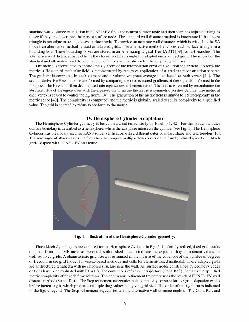
IV. Hemisphere Cylinder AdaptationThe Hemisphere Cylinder geometry is based on a wind tunnel study by Hsieh [41, 42]. For this study, the outer

domain boundary is described as a hemisphere, where the exit plane intersects the cylinder (see Fig. 1). The HemisphereCylinder was previously used for RANS solver verification with a different outer boundary shape and grid topology [6].The zero angle of attack case is the focus here to compare multiple flow solvers on uniformly-refined grids to Lp Machgrids adapted with FUN3D-FV and refine.

Fig. 1 Illustration of the Hemisphere Cylinder geometry.

Three Mach Lp strategies are explored for the Hemisphere Cylinder in Fig. 2. Uniformly-refined, fixed grid resultsobtained from the TMR are also presented with dashed lines to indicate the expected drag component values forwell-resolved grids. A characteristic grid size h is estimated as the inverse of the cube root of the number of degreesof freedom in the grid (nodes for vertex-based methods and cells for element-based methods). These adapted gridsare unstructured tetrahedra with no imposed structure near the wall. All surface nodes constrained by geometry edgesor faces have been evaluated with EGADS. The continuous refinement trajectory (Cont. Ref.) increases the specifiedmetric complexity after each flow solution. The continuous refinement trajectory uses the standard FUN3D-FV walldistance method (Stand. Dist.). The Step refinement trajectories hold complexity constant for five grid adaptation cyclesbefore increasing it, which produces multiple drag values at a given grid size. The order of the Lp norm is indicatedin the figure legend. The Step refinement trajectories use the alternative wall distance method. The Cont. Ref. and

6

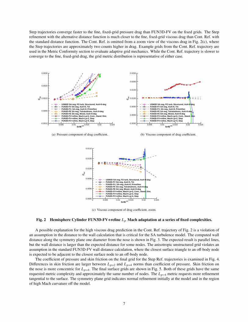
Step trajectories converge faster to the fine, fixed-grid pressure drag than FUN3D-FV on the fixed grids. The Steprefinement with the alternative distance function is much closer to the fine, fixed-grid viscous drag than Cont. Ref. withthe standard distance function. The Cont. Ref. is omitted from a zoom view of the viscous drag in Fig. 2(c), wherethe Step trajectories are approximately two counts higher in drag. Example grids from the Cont. Ref. trajectory areused in the Metric Conformity section to evaluate adaptive grid mechanics. While the Cont. Ref. trajectory is slower toconverge to the fine, fixed-grid drag, the grid metric distribution is representative of either case.

h=N -1/3

CD

p

0 0.005 0.01 0.015 0.02 0.025-0.0010

0.0000

0.0010

0.0020

0.0030

USM3D SA-neg, FO turb, Structured, AoA=0-degFUN3D-FV SA-neg, AoA=0, TetFUN3D-FV, SA-neg, AoA=0, Prism/hexFUN3D-FE SA-neg, Tetrahedrons, AoA=0-degFUN3D-FE SA-neg, Mixed, AoA=0-degFUN3D-FV+refine, Mach-Lp=2, Cont., Stand. Dist.FUN3D-FV+refine, Mach-Lp=2, StepFUN3D-FV+refine, Mach-Lp=4, Step

(a) Pressure component of drag coefficient.

h=N -1/3

CD

v

0 0.005 0.01 0.015 0.02 0.025-0.0050

0.0000

0.0050

0.0100

0.0150

0.0200

0.0250

USM3D SA-neg, FO turb, Structured, AoA=0-degFUN3D-FV SA-neg, AoA=0, TetFUN3D-FV, SA-neg, AoA=0, Prism/hexFUN3D-FE SA-neg, Tetrahedrons, AoA=0-degFUN3D-FE SA-neg, Mixed, AoA=0-degFUN3D-FV+refine, Mach-Lp=2, Cont., Stand. Dist.FUN3D-FV+refine, Mach-Lp=2, StepFUN3D-FV+refine, Mach-Lp=4, Step

(b) Viscous component of drag coefficient.

h=N -1/3

CD

v

0 0.005 0.01 0.015 0.02 0.0250.0085

0.0090

0.0095

0.0100

0.0105

0.0110

USM3D SA-neg, FO turb, Structured, AoA=0-degFUN3D-FV SA-neg, AoA=0, TetFUN3D-FV, SA-neg, AoA=0, Prism/hexFUN3D-FE SA-neg, Tetrahedrons, AoA=0-degFUN3D-FE SA-neg, Mixed, AoA=0-degFUN3D-FV+refine, Mach-Lp=2, Cont., Stand. Dist.FUN3D-FV+refine, Mach-Lp=2, StepFUN3D-FV+refine, Mach-Lp=4, Step

(c) Viscous component of drag coefficient, zoom.

Fig. 2 Hemisphere Cylinder FUN3D-FV+refine Lp Mach adaptation at a series of fixed complexities.

A possible explanation for the high viscous drag prediction in the Cont. Ref. trajectory of Fig. 2 is a violation ofan assumption in the distance to the wall calculation that is critical for the SA turbulence model. The computed walldistance along the symmetry plane one diameter from the nose is shown in Fig. 3. The expected result is parallel lines,but the wall distance is larger than the expected distance for some nodes. The anisotropic unstructured grid violates anassumption in the standard FUN3D-FV wall distance calculation, where the closest surface triangle to an off-body nodeis expected to be adjacent to the closest surface node to an off-body node.

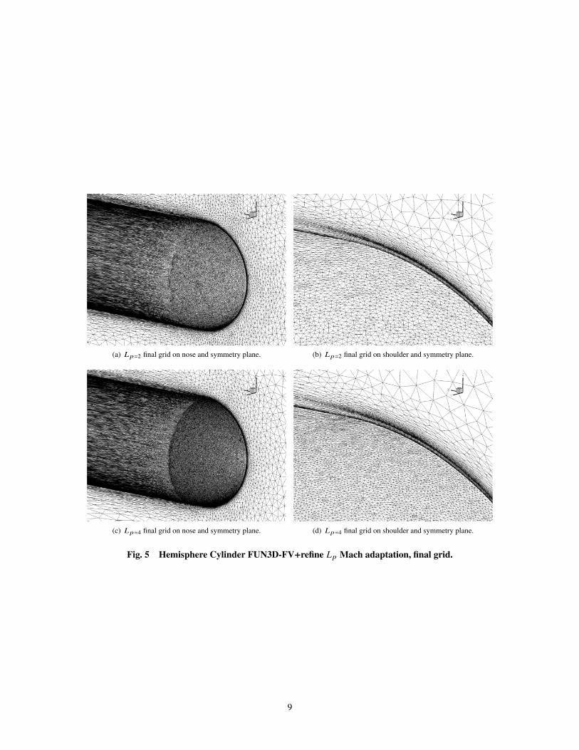
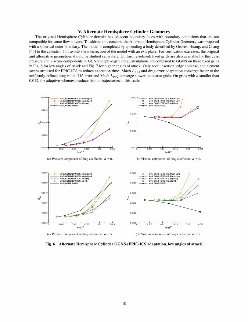
The coefficient of pressure and skin friction on the final grid for the Step Ref. trajectories is examined in Fig. 4.Differences in skin friction are larger between Lp=2 and Lp=4 norms than coefficient of pressure. Skin friction onthe nose is more concentric for Lp=4. The final surface grids are shown in Fig. 5. Both of these grids have the samerequested metric complexity and approximately the same number of nodes. The Lp=4 metric requests more refinementtangential to the surface. The symmetry plane grid indicates normal refinement initially at the model and in the regionof high Mach curvature off the model.

7

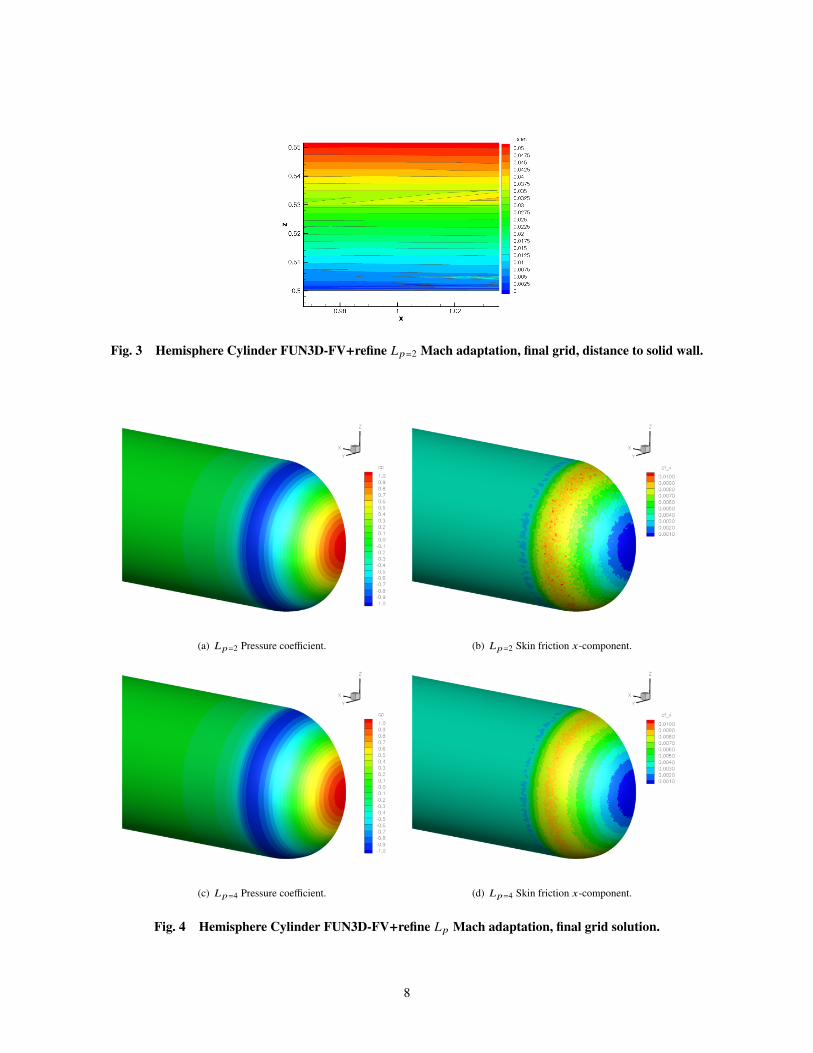
Fig. 3 Hemisphere Cylinder FUN3D-FV+refine Lp=2 Mach adaptation, final grid, distance to solid wall.

(a) Lp=2 Pressure coefficient. (b) Lp=2 Skin friction x-component.

(c) Lp=4 Pressure coefficient. (d) Lp=4 Skin friction x-component.

Fig. 4 Hemisphere Cylinder FUN3D-FV+refine Lp Mach adaptation, final grid solution.

8

(a) Lp=2 final grid on nose and symmetry plane. (b) Lp=2 final grid on shoulder and symmetry plane.

(c) Lp=4 final grid on nose and symmetry plane. (d) Lp=4 final grid on shoulder and symmetry plane.

Fig. 5 Hemisphere Cylinder FUN3D-FV+refine Lp Mach adaptation, final grid.

9

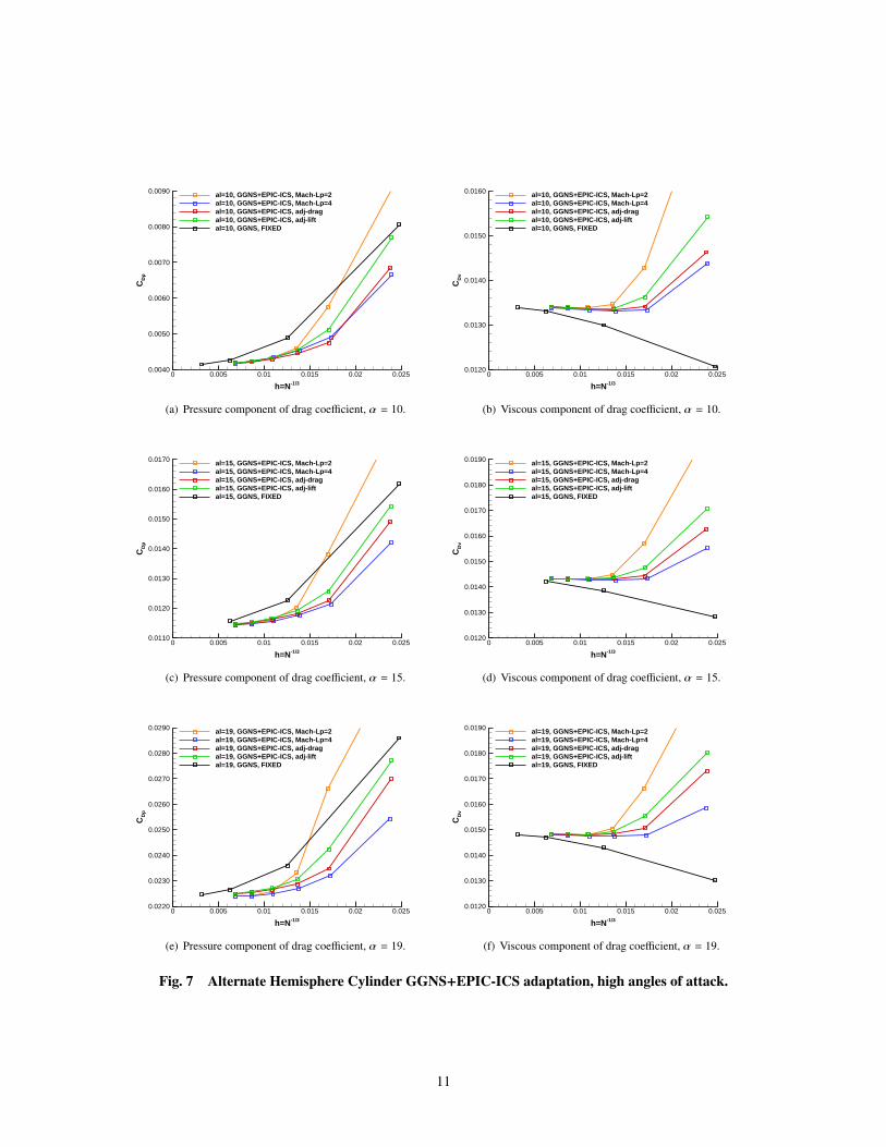
V. Alternate Hemisphere Cylinder GeometryThe original Hemisphere Cylinder domain has adjacent boundary faces with boundary conditions that are not

compatible for some flow solvers. To address this concern, the Alternate Hemisphere Cylinder Geometry was proposedwith a spherical outer boundary. The model is completed by appending a body described by Groves, Huang, and Chang[43] to the cylinder. This avoids the intersection of the model with an exit plane. For verification exercises, the originaland alternative geometries should be studied separately. Uniformly-refined, fixed grids are also available for this case.Pressure and viscous components of GGNS adaptive grid drag calculations are compared to GGNS on these fixed gridsin Fig. 6 for low angles of attack and Fig. 7 for higher angles of attack. Only node insertion, edge collapse, and elementswaps are used for EPIC-ICS to reduce execution time. Mach Lp=4 and drag error adaptation converge faster to theuniformly-refined drag value. Lift error and Mach Lp=2 converge slower on coarse grids. On grids with h smaller than0.012, the adaptive schemes produce similar trajectories at this scale.

h=N -1/3

CD

p

0 0.005 0.01 0.015 0.02 0.0250.0010

0.0020

0.0030

0.0040

0.0050 al=0, GGNS+EPIC-ICS, Mach-Lp=2al=0, GGNS+EPIC-ICS, Mach-Lp=4al=0, GGNS+EPIC-ICS, adj-dragal=0, GGNS, FIXED

(a) Pressure component of drag coefficient, α = 0.

h=N -1/3

CD

v

0 0.005 0.01 0.015 0.02 0.0250.0100

0.0110

0.0120

0.0130 al=0, GGNS+EPIC-ICS, Mach-Lp=2al=0, GGNS+EPIC-ICS, Mach-Lp=4al=0, GGNS+EPIC-ICS, adj-dragal=0, GGNS, FIXED

(b) Viscous component of drag coefficient, α = 0.

h=N -1/3

CD

p

0 0.005 0.01 0.015 0.02 0.0250.0010

0.0020

0.0030

0.0040

0.0050

0.0060 al=5, GGNS+EPIC-ICS, Mach-Lp=2al=5, GGNS+EPIC-ICS, Mach-Lp=4al=5, GGNS+EPIC-ICS, adj-dragal=5, GGNS+EPIC-ICS, adj-liftal=5, GGNS, FIXED

(c) Pressure component of drag coefficient, α = 5.

h=N -1/3

CD

v

0 0.005 0.01 0.015 0.02 0.0250.0100

0.0110

0.0120

0.0130

0.0140

0.0150 al=5, GGNS+EPIC-ICS, Mach-Lp=2al=5, GGNS+EPIC-ICS, Mach-Lp=4al=5, GGNS+EPIC-ICS, adj-dragal=5, GGNS+EPIC-ICS, adj-liftal=5, GGNS, FIXED

(d) Viscous component of drag coefficient, α = 5.

Fig. 6 Alternate Hemisphere Cylinder GGNS+EPIC-ICS adaptation, low angles of attack.

10

h=N -1/3

CD

p

0 0.005 0.01 0.015 0.02 0.0250.0040

0.0050

0.0060

0.0070

0.0080

0.0090 al=10, GGNS+EPIC-ICS, Mach-Lp=2al=10, GGNS+EPIC-ICS, Mach-Lp=4al=10, GGNS+EPIC-ICS, adj-dragal=10, GGNS+EPIC-ICS, adj-liftal=10, GGNS, FIXED

(a) Pressure component of drag coefficient, α = 10.

h=N -1/3

CD

v

0 0.005 0.01 0.015 0.02 0.0250.0120

0.0130

0.0140

0.0150

0.0160 al=10, GGNS+EPIC-ICS, Mach-Lp=2al=10, GGNS+EPIC-ICS, Mach-Lp=4al=10, GGNS+EPIC-ICS, adj-dragal=10, GGNS+EPIC-ICS, adj-liftal=10, GGNS, FIXED

(b) Viscous component of drag coefficient, α = 10.

h=N -1/3

CD

p

0 0.005 0.01 0.015 0.02 0.0250.0110

0.0120

0.0130

0.0140

0.0150

0.0160

0.0170 al=15, GGNS+EPIC-ICS, Mach-Lp=2al=15, GGNS+EPIC-ICS, Mach-Lp=4al=15, GGNS+EPIC-ICS, adj-dragal=15, GGNS+EPIC-ICS, adj-liftal=15, GGNS, FIXED

(c) Pressure component of drag coefficient, α = 15.

h=N -1/3

CD

v

0 0.005 0.01 0.015 0.02 0.0250.0120

0.0130

0.0140

0.0150

0.0160

0.0170

0.0180

0.0190 al=15, GGNS+EPIC-ICS, Mach-Lp=2al=15, GGNS+EPIC-ICS, Mach-Lp=4al=15, GGNS+EPIC-ICS, adj-dragal=15, GGNS+EPIC-ICS, adj-liftal=15, GGNS, FIXED

(d) Viscous component of drag coefficient, α = 15.

h=N -1/3

CD

p

0 0.005 0.01 0.015 0.02 0.0250.0220

0.0230

0.0240

0.0250

0.0260

0.0270

0.0280

0.0290 al=19, GGNS+EPIC-ICS, Mach-Lp=2al=19, GGNS+EPIC-ICS, Mach-Lp=4al=19, GGNS+EPIC-ICS, adj-dragal=19, GGNS+EPIC-ICS, adj-liftal=19, GGNS, FIXED

(e) Pressure component of drag coefficient, α = 19.

h=N -1/3

CD

v

0 0.005 0.01 0.015 0.02 0.0250.0120

0.0130

0.0140

0.0150

0.0160

0.0170

0.0180

0.0190 al=19, GGNS+EPIC-ICS, Mach-Lp=2al=19, GGNS+EPIC-ICS, Mach-Lp=4al=19, GGNS+EPIC-ICS, adj-dragal=19, GGNS+EPIC-ICS, adj-liftal=19, GGNS, FIXED

(f) Viscous component of drag coefficient, α = 19.

Fig. 7 Alternate Hemisphere Cylinder GGNS+EPIC-ICS adaptation, high angles of attack.

11

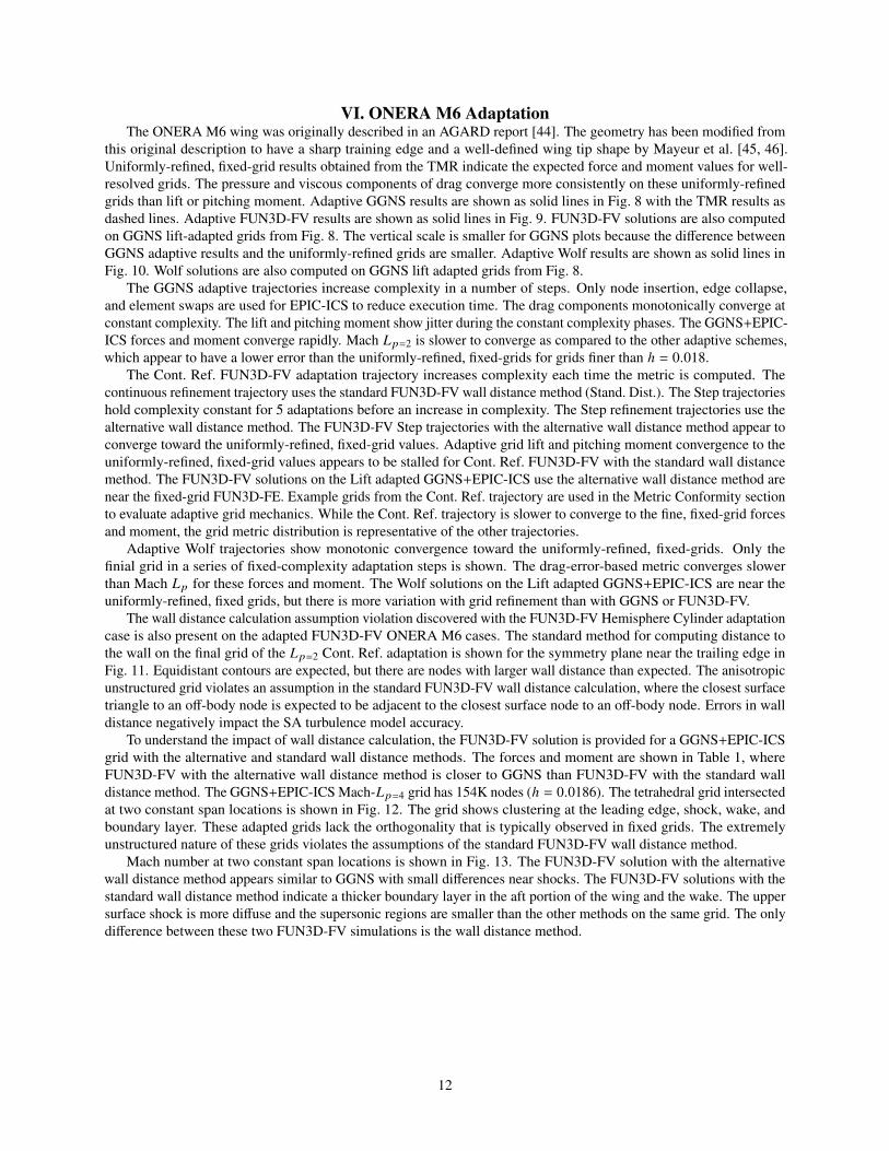
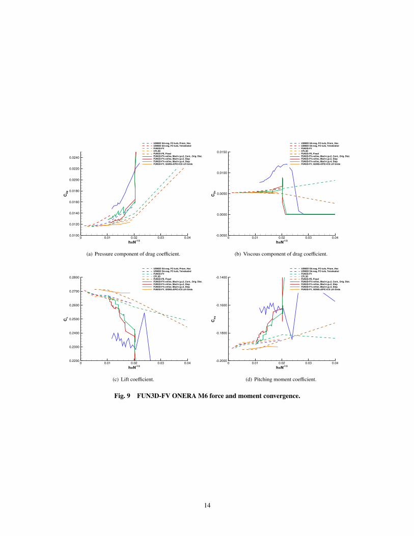
VI. ONERA M6 AdaptationThe ONERA M6 wing was originally described in an AGARD report [44]. The geometry has been modified from

this original description to have a sharp training edge and a well-defined wing tip shape by Mayeur et al. [45, 46].Uniformly-refined, fixed-grid results obtained from the TMR indicate the expected force and moment values for well-resolved grids. The pressure and viscous components of drag converge more consistently on these uniformly-refinedgrids than lift or pitching moment. Adaptive GGNS results are shown as solid lines in Fig. 8 with the TMR results asdashed lines. Adaptive FUN3D-FV results are shown as solid lines in Fig. 9. FUN3D-FV solutions are also computedon GGNS lift-adapted grids from Fig. 8. The vertical scale is smaller for GGNS plots because the difference betweenGGNS adaptive results and the uniformly-refined grids are smaller. Adaptive Wolf results are shown as solid lines inFig. 10. Wolf solutions are also computed on GGNS lift adapted grids from Fig. 8.

The GGNS adaptive trajectories increase complexity in a number of steps. Only node insertion, edge collapse,and element swaps are used for EPIC-ICS to reduce execution time. The drag components monotonically converge atconstant complexity. The lift and pitching moment show jitter during the constant complexity phases. The GGNS+EPIC-ICS forces and moment converge rapidly. Mach Lp=2 is slower to converge as compared to the other adaptive schemes,which appear to have a lower error than the uniformly-refined, fixed-grids for grids finer than h = 0.018.

The Cont. Ref. FUN3D-FV adaptation trajectory increases complexity each time the metric is computed. Thecontinuous refinement trajectory uses the standard FUN3D-FV wall distance method (Stand. Dist.). The Step trajectorieshold complexity constant for 5 adaptations before an increase in complexity. The Step refinement trajectories use thealternative wall distance method. The FUN3D-FV Step trajectories with the alternative wall distance method appear toconverge toward the uniformly-refined, fixed-grid values. Adaptive grid lift and pitching moment convergence to theuniformly-refined, fixed-grid values appears to be stalled for Cont. Ref. FUN3D-FV with the standard wall distancemethod. The FUN3D-FV solutions on the Lift adapted GGNS+EPIC-ICS use the alternative wall distance method arenear the fixed-grid FUN3D-FE. Example grids from the Cont. Ref. trajectory are used in the Metric Conformity sectionto evaluate adaptive grid mechanics. While the Cont. Ref. trajectory is slower to converge to the fine, fixed-grid forcesand moment, the grid metric distribution is representative of the other trajectories.

Adaptive Wolf trajectories show monotonic convergence toward the uniformly-refined, fixed-grids. Only thefinial grid in a series of fixed-complexity adaptation steps is shown. The drag-error-based metric converges slowerthan Mach Lp for these forces and moment. The Wolf solutions on the Lift adapted GGNS+EPIC-ICS are near theuniformly-refined, fixed grids, but there is more variation with grid refinement than with GGNS or FUN3D-FV.

The wall distance calculation assumption violation discovered with the FUN3D-FV Hemisphere Cylinder adaptationcase is also present on the adapted FUN3D-FV ONERA M6 cases. The standard method for computing distance tothe wall on the final grid of the Lp=2 Cont. Ref. adaptation is shown for the symmetry plane near the trailing edge inFig. 11. Equidistant contours are expected, but there are nodes with larger wall distance than expected. The anisotropicunstructured grid violates an assumption in the standard FUN3D-FV wall distance calculation, where the closest surfacetriangle to an off-body node is expected to be adjacent to the closest surface node to an off-body node. Errors in walldistance negatively impact the SA turbulence model accuracy.

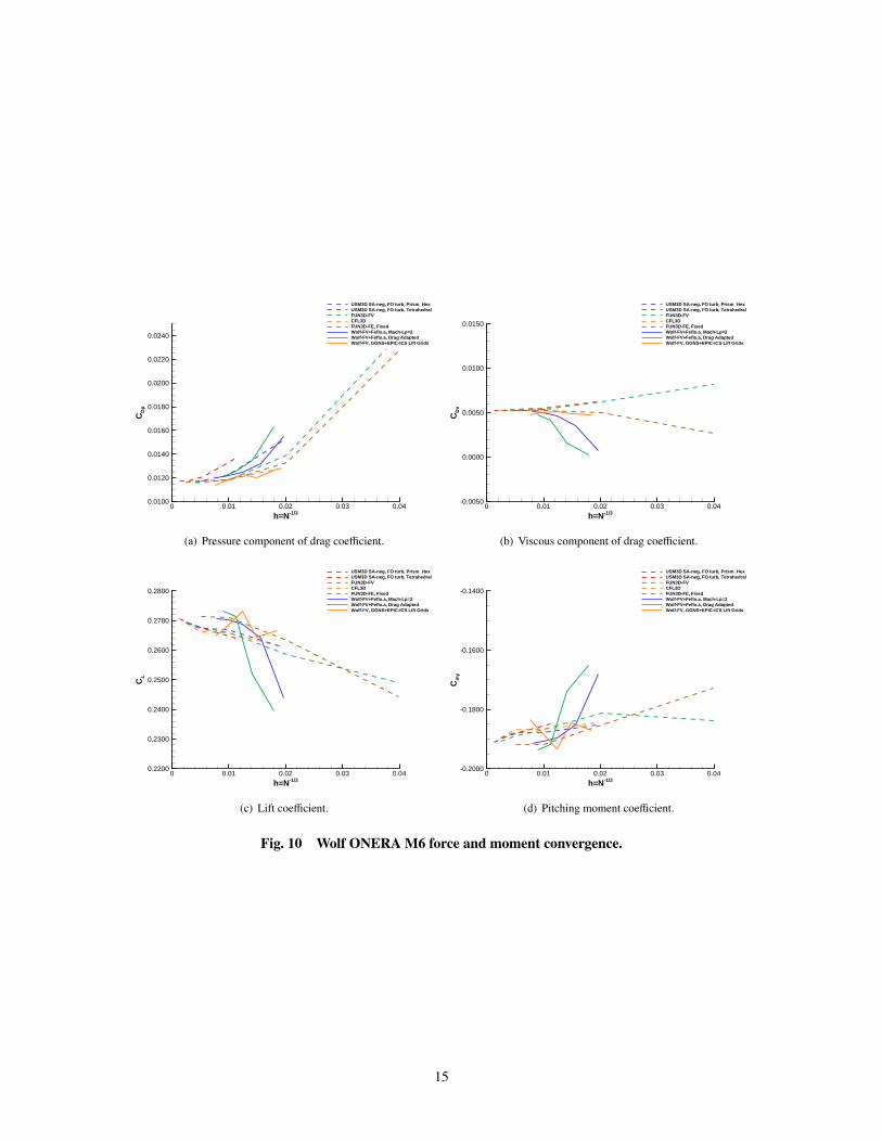
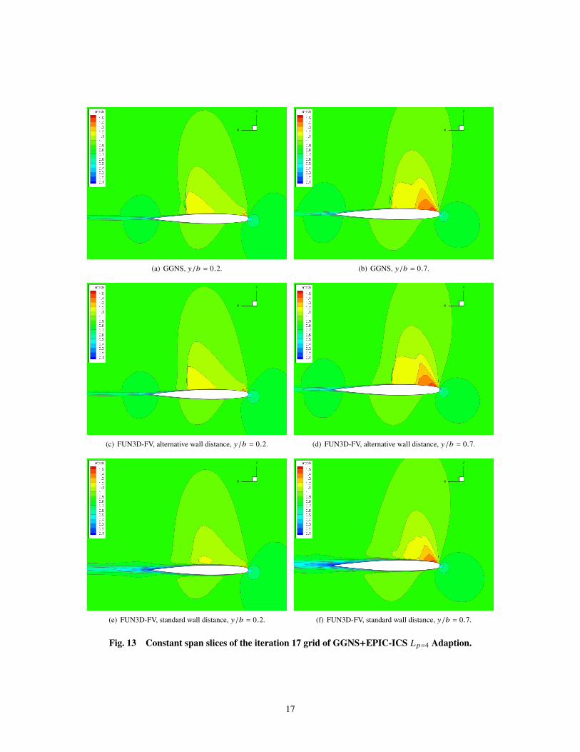
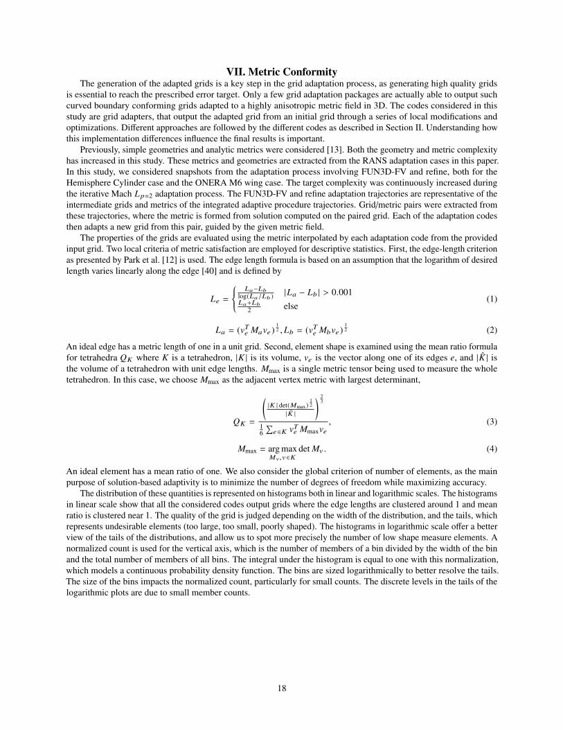
To understand the impact of wall distance calculation, the FUN3D-FV solution is provided for a GGNS+EPIC-ICSgrid with the alternative and standard wall distance methods. The forces and moment are shown in Table 1, whereFUN3D-FV with the alternative wall distance method is closer to GGNS than FUN3D-FV with the standard walldistance method. The GGNS+EPIC-ICS Mach-Lp=4 grid has 154K nodes (h = 0.0186). The tetrahedral grid intersectedat two constant span locations is shown in Fig. 12. The grid shows clustering at the leading edge, shock, wake, andboundary layer. These adapted grids lack the orthogonality that is typically observed in fixed grids. The extremelyunstructured nature of these grids violates the assumptions of the standard FUN3D-FV wall distance method.

Mach number at two constant span locations is shown in Fig. 13. The FUN3D-FV solution with the alternativewall distance method appears similar to GGNS with small differences near shocks. The FUN3D-FV solutions with thestandard wall distance method indicate a thicker boundary layer in the aft portion of the wing and the wake. The uppersurface shock is more diffuse and the supersonic regions are smaller than the other methods on the same grid. The onlydifference between these two FUN3D-FV simulations is the wall distance method.

12

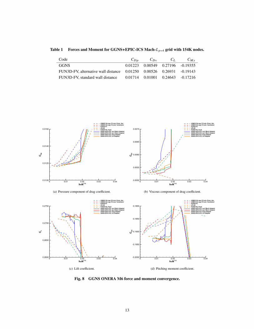
Table 1 Forces and Moment for GGNS+EPIC-ICS Mach-Lp=4 grid with 154K nodes.

Code CDp CDv CL CMy

GGNS 0.01223 0.00549 0.27196 -0.19355FUN3D-FV, alternative wall distance 0.01250 0.00526 0.26931 -0.19143FUN3D-FV, standard wall distance 0.01714 0.01001 0.24643 -0.17216

h=N­1/3

CD

p

0 0.01 0.02 0.03 0.040.0100

0.0120

0.0140

0.0160

USM3D SA­neg, FO turb, Prism_Hex

USM3D SA­neg, FO turb, Tetrahedral

FUN3D­FV

CFL3D

FUN3D­FE, Fixed

GGNS+EPIC­ICS, Lp=2 Mach Adapted

GGNS+EPIC­ICS, Lp=4 Mach Adapted

GGNS+EPIC­ICS, Drag AdaptedGGNS+EPIC­ICS, Lift Adapted

(a) Pressure component of drag coefficient.

h=N­1/3

CD

v

0 0.01 0.02 0.03 0.040.0050

0.0055

0.0060

0.0065

0.0070

USM3D SA­neg, FO turb, Prism_Hex

USM3D SA­neg, FO turb, Tetrahedral

FUN3D­FV

CFL3D

FUN3D­FE, Fixed

GGNS+EPIC­ICS, Lp=2 Mach Adapted

GGNS+EPIC­ICS, Lp=4 Mach Adapted

GGNS+EPIC­ICS, Drag AdaptedGGNS+EPIC­ICS, Lift Adapted

(b) Viscous component of drag coefficient.

h=N­1/3

CL

0 0.01 0.02 0.03 0.040.2600

0.2650

0.2700

0.2750

USM3D SA­neg, FO turb, Prism_Hex

USM3D SA­neg, FO turb, Tetrahedral

FUN3D­FV

CFL3D

FUN3D­FE, Fixed

GGNS+EPIC­ICS, Lp=2 Mach Adapted

GGNS+EPIC­ICS, Lp=4 Mach Adapted

GGNS+EPIC­ICS, Drag AdaptedGGNS+EPIC­ICS, Lift Adapted

(c) Lift coefficient.

h=N­1/3

Cm

y

0 0.01 0.02 0.03 0.04­0.2000

­0.1950

­0.1900

­0.1850

­0.1800

USM3D SA­neg, FO turb, Prism_Hex

USM3D SA­neg, FO turb, Tetrahedral

FUN3D­FV

CFL3D

FUN3D­FE, Fixed

GGNS+EPIC­ICS, Lp=2 Mach Adapted

GGNS+EPIC­ICS, Lp=4 Mach Adapted

GGNS+EPIC­ICS, Drag AdaptedGGNS+EPIC­ICS, Lift Adapted

(d) Pitching moment coefficient.

Fig. 8 GGNS ONERA M6 force and moment convergence.

13

h=N­1/3

CD

p

0 0.01 0.02 0.03 0.040.0100

0.0120

0.0140

0.0160

0.0180

0.0200

0.0220

0.0240

USM3D SA­neg, FO turb, Prism_Hex

USM3D SA­neg, FO turb, Tetrahedral

FUN3D­FV

CFL3D

FUN3D­FE, Fixed

FUN3D­FV+refine, Mach­Lp=2, Cont., Orig. Dist.

FUN3D­FV+refine, Mach­Lp=2, Step

FUN3D­FV+refine, Mach­Lp=4, Step

FUN3D­FV, GGNS+EPIC­ICS Lift Grids

(a) Pressure component of drag coefficient.

h=N­1/3

CD

v

0 0.01 0.02 0.03 0.04­0.0050

0.0000

0.0050

0.0100

0.0150

USM3D SA­neg, FO turb, Prism_Hex

USM3D SA­neg, FO turb, Tetrahedral

FUN3D­FV

CFL3D

FUN3D­FE, Fixed

FUN3D­FV+refine, Mach­Lp=2, Cont., Orig. Dist.

FUN3D­FV+refine, Mach­Lp=2, Step

FUN3D­FV+refine, Mach­Lp=4, Step

FUN3D­FV, GGNS+EPIC­ICS Lift Grids

(b) Viscous component of drag coefficient.

h=N­1/3

CL

0 0.01 0.02 0.03 0.040.2200

0.2300

0.2400

0.2500

0.2600

0.2700

0.2800

USM3D SA­neg, FO turb, Prism_Hex

USM3D SA­neg, FO turb, Tetrahedral

FUN3D­FV

CFL3D

FUN3D­FE, Fixed

FUN3D­FV+refine, Mach­Lp=2, Cont., Orig. Dist.

FUN3D­FV+refine, Mach­Lp=2, Step

FUN3D­FV+refine, Mach­Lp=4, Step

FUN3D­FV, GGNS+EPIC­ICS Lift Grids

(c) Lift coefficient.

h=N­1/3

Cm

y

0 0.01 0.02 0.03 0.04­0.2000

­0.1800

­0.1600

­0.1400

USM3D SA­neg, FO turb, Prism_Hex

USM3D SA­neg, FO turb, Tetrahedral

FUN3D­FV

CFL3D

FUN3D­FE, Fixed

FUN3D­FV+refine, Mach­Lp=2, Cont., Orig. Dist.

FUN3D­FV+refine, Mach­Lp=2, Step

FUN3D­FV+refine, Mach­Lp=4, Step

FUN3D­FV, GGNS+EPIC­ICS Lift Grids

(d) Pitching moment coefficient.

Fig. 9 FUN3D-FV ONERA M6 force and moment convergence.

14

h=N -1/3

CD

p

0 0.01 0.02 0.03 0.040.0100

0.0120

0.0140

0.0160

0.0180

0.0200

0.0220

0.0240

USM3D SA-neg, FO turb, Prism_HexUSM3D SA-neg, FO turb, TetrahedralFUN3D-FVCFL3DFUN3D-FE, FixedWolf-FV+Feflo.a, Mach-Lp=2Wolf-FV+Feflo.a, Drag AdaptedWolf-FV, GGNS+EPIC-ICS Lift Grids

(a) Pressure component of drag coefficient.

h=N -1/3

CD

v

0 0.01 0.02 0.03 0.04-0.0050

0.0000

0.0050

0.0100

0.0150

USM3D SA-neg, FO turb, Prism_HexUSM3D SA-neg, FO turb, TetrahedralFUN3D-FVCFL3DFUN3D-FE, FixedWolf-FV+Feflo.a, Mach-Lp=2Wolf-FV+Feflo.a, Drag AdaptedWolf-FV, GGNS+EPIC-ICS Lift Grids

(b) Viscous component of drag coefficient.

h=N -1/3

CL

0 0.01 0.02 0.03 0.040.2200

0.2300

0.2400

0.2500

0.2600

0.2700

0.2800

USM3D SA-neg, FO turb, Prism_HexUSM3D SA-neg, FO turb, TetrahedralFUN3D-FVCFL3DFUN3D-FE, FixedWolf-FV+Feflo.a, Mach-Lp=2Wolf-FV+Feflo.a, Drag AdaptedWolf-FV, GGNS+EPIC-ICS Lift Grids

(c) Lift coefficient.

h=N -1/3

Cm

y

0 0.01 0.02 0.03 0.04-0.2000

-0.1800

-0.1600

-0.1400

USM3D SA-neg, FO turb, Prism_HexUSM3D SA-neg, FO turb, TetrahedralFUN3D-FVCFL3DFUN3D-FE, FixedWolf-FV+Feflo.a, Mach-Lp=2Wolf-FV+Feflo.a, Drag AdaptedWolf-FV, GGNS+EPIC-ICS Lift Grids

(d) Pitching moment coefficient.

Fig. 10 Wolf ONERA M6 force and moment convergence.

15

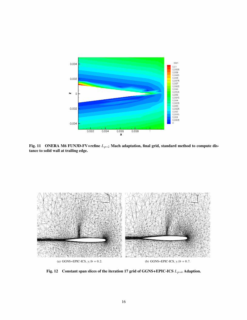
Fig. 11 ONERA M6 FUN3D-FV+refine Lp=2 Mach adaptation, final grid, standard method to compute dis-tance to solid wall at trailing edge.

(a) GGNS+EPIC-ICS, y/b = 0.2. (b) GGNS+EPIC-ICS, y/b = 0.7.

Fig. 12 Constant span slices of the iteration 17 grid of GGNS+EPIC-ICS Lp=4 Adaption.

16

(a) GGNS, y/b = 0.2. (b) GGNS, y/b = 0.7.

(c) FUN3D-FV, alternative wall distance, y/b = 0.2. (d) FUN3D-FV, alternative wall distance, y/b = 0.7.

(e) FUN3D-FV, standard wall distance, y/b = 0.2. (f) FUN3D-FV, standard wall distance, y/b = 0.7.

Fig. 13 Constant span slices of the iteration 17 grid of GGNS+EPIC-ICS Lp=4 Adaption.

17

VII. Metric ConformityThe generation of the adapted grids is a key step in the grid adaptation process, as generating high quality grids

is essential to reach the prescribed error target. Only a few grid adaptation packages are actually able to output suchcurved boundary conforming grids adapted to a highly anisotropic metric field in 3D. The codes considered in thisstudy are grid adapters, that output the adapted grid from an initial grid through a series of local modifications andoptimizations. Different approaches are followed by the different codes as described in Section II. Understanding howthis implementation differences influence the final results is important.

Previously, simple geometries and analytic metrics were considered [13]. Both the geometry and metric complexityhas increased in this study. These metrics and geometries are extracted from the RANS adaptation cases in this paper.In this study, we considered snapshots from the adaptation process involving FUN3D-FV and refine, both for theHemisphere Cylinder case and the ONERA M6 wing case. The target complexity was continuously increased duringthe iterative Mach Lp=2 adaptation process. The FUN3D-FV and refine adaptation trajectories are representative of theintermediate grids and metrics of the integrated adaptive procedure trajectories. Grid/metric pairs were extracted fromthese trajectories, where the metric is formed from solution computed on the paired grid. Each of the adaptation codesthen adapts a new grid from this pair, guided by the given metric field.

The properties of the grids are evaluated using the metric interpolated by each adaptation code from the providedinput grid. Two local criteria of metric satisfaction are employed for descriptive statistics. First, the edge-length criterionas presented by Park et al. [12] is used. The edge length formula is based on an assumption that the logarithm of desiredlength varies linearly along the edge [40] and is defined by

Le =

La−Lb

log(La/Lb ) |La − Lb | > 0.001La+Lb

2 else(1)

La = (vTe Mave )12 ,Lb = (vTe Mbve )

12 (2)

An ideal edge has a metric length of one in a unit grid. Second, element shape is examined using the mean ratio formulafor tetrahedra QK where K is a tetrahedron, |K | is its volume, ve is the vector along one of its edges e, and |K̂ | isthe volume of a tetrahedron with unit edge lengths. Mmax is a single metric tensor being used to measure the wholetetrahedron. In this case, we choose Mmax as the adjacent vertex metric with largest determinant,

QK =

(|K | det(Mmax)

12

|K̂ |

) 23

16∑

e∈K vTe Mmaxve, (3)

Mmax = arg maxMv,v∈K

det Mv . (4)

An ideal element has a mean ratio of one. We also consider the global criterion of number of elements, as the mainpurpose of solution-based adaptivity is to minimize the number of degrees of freedom while maximizing accuracy.

The distribution of these quantities is represented on histograms both in linear and logarithmic scales. The histogramsin linear scale show that all the considered codes output grids where the edge lengths are clustered around 1 and meanratio is clustered near 1. The quality of the grid is judged depending on the width of the distribution, and the tails, whichrepresents undesirable elements (too large, too small, poorly shaped). The histograms in logarithmic scale offer a betterview of the tails of the distributions, and allow us to spot more precisely the number of low shape measure elements. Anormalized count is used for the vertical axis, which is the number of members of a bin divided by the width of the binand the total number of members of all bins. The integral under the histogram is equal to one with this normalization,which models a continuous probability density function. The bins are sized logarithmically to better resolve the tails.The size of the bins impacts the normalized count, particularly for small counts. The discrete levels in the tails of thelogarithmic plots are due to small member counts.

18

A. Hemisphere Cylinder Metric ConformityTwo versions of this grid/metric pair are taken at different iterations of the adaptation process. The first metric has a

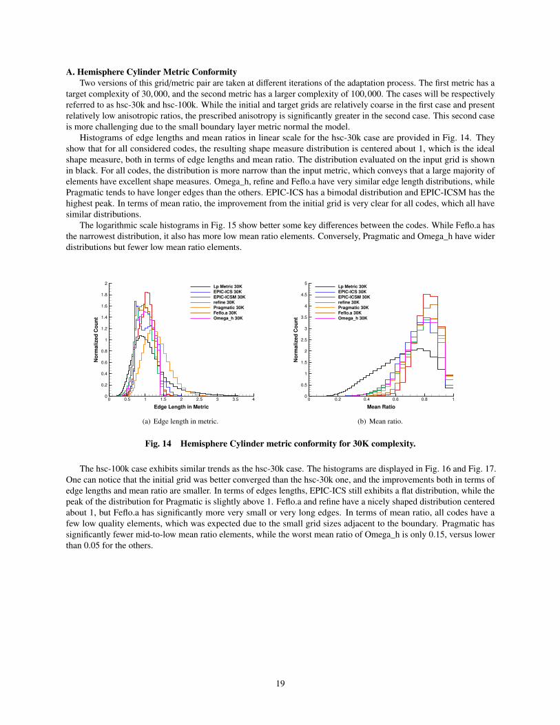
target complexity of 30,000, and the second metric has a larger complexity of 100,000. The cases will be respectivelyreferred to as hsc-30k and hsc-100k. While the initial and target grids are relatively coarse in the first case and presentrelatively low anisotropic ratios, the prescribed anisotropy is significantly greater in the second case. This second caseis more challenging due to the small boundary layer metric normal the model.

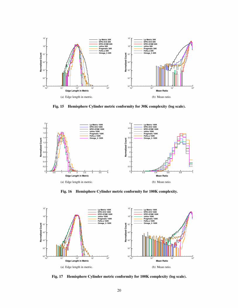
Histograms of edge lengths and mean ratios in linear scale for the hsc-30k case are provided in Fig. 14. Theyshow that for all considered codes, the resulting shape measure distribution is centered about 1, which is the idealshape measure, both in terms of edge lengths and mean ratio. The distribution evaluated on the input grid is shownin black. For all codes, the distribution is more narrow than the input metric, which conveys that a large majority ofelements have excellent shape measures. Omega_h, refine and Feflo.a have very similar edge length distributions, whilePragmatic tends to have longer edges than the others. EPIC-ICS has a bimodal distribution and EPIC-ICSM has thehighest peak. In terms of mean ratio, the improvement from the initial grid is very clear for all codes, which all havesimilar distributions.

The logarithmic scale histograms in Fig. 15 show better some key differences between the codes. While Feflo.a hasthe narrowest distribution, it also has more low mean ratio elements. Conversely, Pragmatic and Omega_h have widerdistributions but fewer low mean ratio elements.

Edge Length in Metric

No

rma

lize

d C

ou

nt

0 0.5 1 1.5 2 2.5 3 3.5 40

0.2

0.4

0.6

0.8

1

1.2

1.4

1.6

1.8

2Lp Metric 30K

EPIC­ICS 30K

EPIC­ICSM 30K

refine 30K

Pragmatic 30K

Feflo.a 30K

Omega_h 30K

(a) Edge length in metric.

Mean Ratio

No

rma

lize

d C

ou

nt

0 0.2 0.4 0.6 0.8 10

0.5

1

1.5

2

2.5

3

3.5

4

4.5

5Lp Metric 30K

EPIC­ICS 30K

EPIC­ICSM 30K

refine 30K

Pragmatic 30K

Feflo.a 30K

Omega_h 30K

(b) Mean ratio.

Fig. 14 Hemisphere Cylinder metric conformity for 30K complexity.

The hsc-100k case exhibits similar trends as the hsc-30k case. The histograms are displayed in Fig. 16 and Fig. 17.One can notice that the initial grid was better converged than the hsc-30k one, and the improvements both in terms ofedge lengths and mean ratio are smaller. In terms of edges lengths, EPIC-ICS still exhibits a flat distribution, while thepeak of the distribution for Pragmatic is slightly above 1. Feflo.a and refine have a nicely shaped distribution centeredabout 1, but Feflo.a has significantly more very small or very long edges. In terms of mean ratio, all codes have afew low quality elements, which was expected due to the small grid sizes adjacent to the boundary. Pragmatic hassignificantly fewer mid-to-low mean ratio elements, while the worst mean ratio of Omega_h is only 0.15, versus lowerthan 0.05 for the others.

19

Edge Length in Metric

No

rma

lize

d C

ou

nt

10­2

10­1

100

101

102

10­5

10­4

10­3

10­2

10­1

100

101

Lp Metric 30K

EPIC­ICS 30K

EPIC­ICSM 30K

refine 30K

Pragmatic 30K

Feflo.a 30K

Omega_h 30K

(a) Edge length in metric.

Mean Ratio

No

rma

lize

d C

ou

nt

10­3

10­2

10­1

100

10­5

10­4

10­3

10­2

10­1

100

101

Lp Metric 30K

EPIC­ICS 30K

EPIC­ICSM 30K

refine 30K

Pragmatic 30K

Feflo.a 30K

Omega_h 30K

(b) Mean ratio.

Fig. 15 Hemisphere Cylinder metric conformity for 30K complexity (log scale).

Edge Length in Metric

No

rma

lize

d C

ou

nt

0 0.5 1 1.5 2 2.5 3 3.5 40

0.2

0.4

0.6

0.8

1

1.2

1.4

1.6

1.8

2Lp Metric 100K

EPIC­ICS 100K

EPIC­ICSM 100K

refine 100K

Pragmatic 100K

Feflo.a 100K

Omega_h 100K

(a) Edge length in metric.

Mean Ratio

No

rma

lize

d C

ou

nt

0 0.2 0.4 0.6 0.8 10

0.5

1

1.5

2

2.5

3

3.5

4

4.5

5Lp Metric 100K

EPIC­ICS 100K

EPIC­ICSM 100K

refine 100K

Pragmatic 100K

Feflo.a 100K

Omega_h 100K

(b) Mean ratio.

Fig. 16 Hemisphere Cylinder metric conformity for 100K complexity.

Edge Length in Metric

No

rma

lize

d C

ou

nt

10­2

10­1

100

101

102

10­5

10­4

10­3

10­2

10­1

100

101

Lp Metric 100K

EPIC­ICS 100K

EPIC­ICSM 100K

refine 100K

Pragmatic 100K

Feflo.a 100K

Omega_h 100K

(a) Edge length in metric.

Mean Ratio

No

rma

lize

d C

ou

nt

10­3

10­2

10­1

100

10­5

10­4

10­3

10­2

10­1

100

101

Lp Metric 100K

EPIC­ICS 100K

EPIC­ICSM 100K

refine 100K

Pragmatic 100K

Feflo.a 100K

Omega_h 100K

(b) Mean ratio.

Fig. 17 Hemisphere Cylinder metric conformity for 100K complexity (log scale).

20

B. ONERA M6 Metric ConformityGrid/metric pairs from the ONERA M6 wing FUN3D-FV+refine Mach Lp=2 continuous refinement trajectory are

also adapted. Two versions of this case are considered, with metric complexities of 30,000 and 100,000. The cases willbe respectively referred to as m6-30k and m6-100k. The geometry of this case is more complex than for the hemispherecylinder, and the very thin anisotropic boundary layer is expected to be a challenge, notably close to the tip and thetrailing edge of the wing.

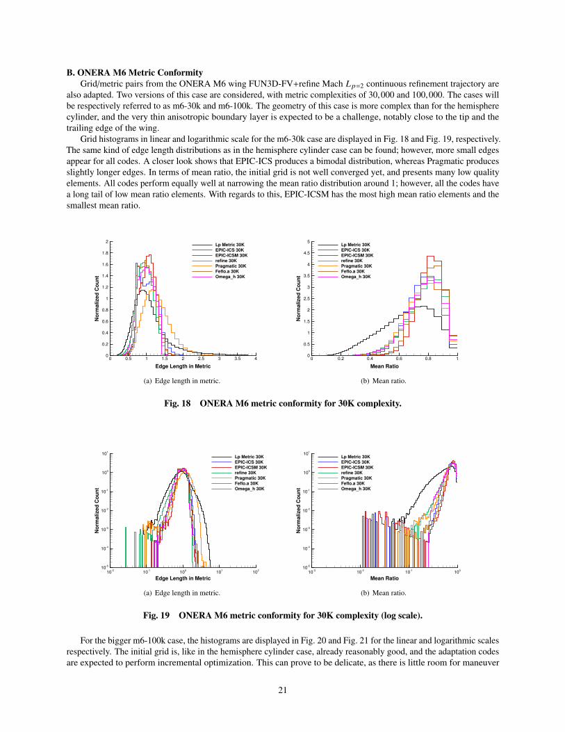
Grid histograms in linear and logarithmic scale for the m6-30k case are displayed in Fig. 18 and Fig. 19, respectively.The same kind of edge length distributions as in the hemisphere cylinder case can be found; however, more small edgesappear for all codes. A closer look shows that EPIC-ICS produces a bimodal distribution, whereas Pragmatic producesslightly longer edges. In terms of mean ratio, the initial grid is not well converged yet, and presents many low qualityelements. All codes perform equally well at narrowing the mean ratio distribution around 1; however, all the codes havea long tail of low mean ratio elements. With regards to this, EPIC-ICSM has the most high mean ratio elements and thesmallest mean ratio.

Edge Length in Metric

No

rma

lize

d C

ou

nt

0 0.5 1 1.5 2 2.5 3 3.5 40

0.2

0.4

0.6

0.8

1

1.2

1.4

1.6

1.8

2Lp Metric 30K

EPIC­ICS 30K

EPIC­ICSM 30K

refine 30K

Pragmatic 30K

Feflo.a 30K

Omega_h 30K

(a) Edge length in metric.

Mean Ratio

No

rma

lize

d C

ou

nt

0 0.2 0.4 0.6 0.8 10

0.5

1

1.5

2

2.5

3

3.5

4

4.5

5Lp Metric 30K

EPIC­ICS 30K

EPIC­ICSM 30K

refine 30K

Pragmatic 30K

Feflo.a 30K

Omega_h 30K

(b) Mean ratio.

Fig. 18 ONERA M6 metric conformity for 30K complexity.

Edge Length in Metric

No

rma

lize

d C

ou

nt

10­2

10­1

100

101

102

10­5

10­4

10­3

10­2

10­1

100

101

Lp Metric 30K

EPIC­ICS 30K

EPIC­ICSM 30K

refine 30K

Pragmatic 30K

Feflo.a 30K

Omega_h 30K

(a) Edge length in metric.

Mean Ratio

No

rma

lize

d C

ou

nt

10­3

10­2

10­1

100

10­5

10­4

10­3

10­2

10­1

100

101

Lp Metric 30K

EPIC­ICS 30K

EPIC­ICSM 30K

refine 30K

Pragmatic 30K

Feflo.a 30K

Omega_h 30K

(b) Mean ratio.

Fig. 19 ONERA M6 metric conformity for 30K complexity (log scale).

For the bigger m6-100k case, the histograms are displayed in Fig. 20 and Fig. 21 for the linear and logarithmic scalesrespectively. The initial grid is, like in the hemisphere cylinder case, already reasonably good, and the adaptation codesare expected to perform incremental optimization. This can prove to be delicate, as there is little room for maneuver

21

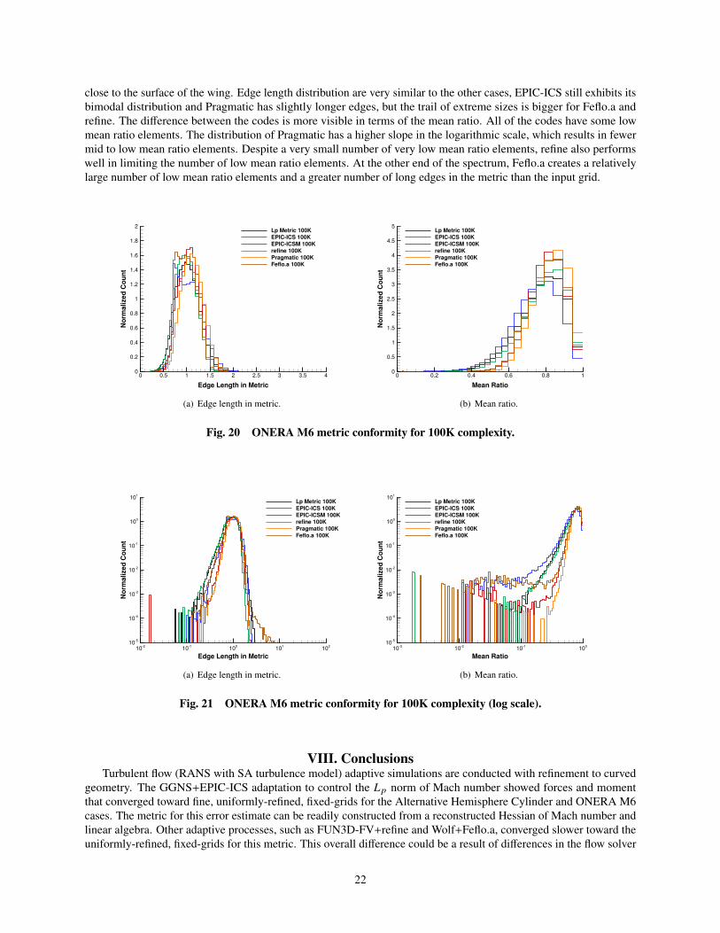
close to the surface of the wing. Edge length distribution are very similar to the other cases, EPIC-ICS still exhibits itsbimodal distribution and Pragmatic has slightly longer edges, but the trail of extreme sizes is bigger for Feflo.a andrefine. The difference between the codes is more visible in terms of the mean ratio. All of the codes have some lowmean ratio elements. The distribution of Pragmatic has a higher slope in the logarithmic scale, which results in fewermid to low mean ratio elements. Despite a very small number of very low mean ratio elements, refine also performswell in limiting the number of low mean ratio elements. At the other end of the spectrum, Feflo.a creates a relativelylarge number of low mean ratio elements and a greater number of long edges in the metric than the input grid.

Edge Length in Metric

No

rma

lize

d C

ou

nt

0 0.5 1 1.5 2 2.5 3 3.5 40

0.2

0.4

0.6

0.8

1

1.2

1.4

1.6

1.8

2Lp Metric 100K

EPIC­ICS 100K

EPIC­ICSM 100K

refine 100K

Pragmatic 100K

Feflo.a 100K

(a) Edge length in metric.

Mean RatioN

orm

alize

d C

ou

nt

0 0.2 0.4 0.6 0.8 10

0.5

1

1.5

2

2.5

3

3.5

4

4.5

5Lp Metric 100K

EPIC­ICS 100K

EPIC­ICSM 100K

refine 100K

Pragmatic 100K

Feflo.a 100K

(b) Mean ratio.

Fig. 20 ONERA M6 metric conformity for 100K complexity.

Edge Length in Metric

No

rma

lize

d C

ou

nt

10­2

10­1

100

101

102

10­5

10­4

10­3

10­2

10­1

100

101

Lp Metric 100K

EPIC­ICS 100K

EPIC­ICSM 100K

refine 100K

Pragmatic 100K

Feflo.a 100K

(a) Edge length in metric.

Mean Ratio

No

rma

lize

d C

ou

nt

10­3

10­2

10­1

100

10­5

10­4

10­3

10­2

10­1

100

101

Lp Metric 100K

EPIC­ICS 100K

EPIC­ICSM 100K

refine 100K

Pragmatic 100K

Feflo.a 100K

(b) Mean ratio.

Fig. 21 ONERA M6 metric conformity for 100K complexity (log scale).

VIII. ConclusionsTurbulent flow (RANS with SA turbulence model) adaptive simulations are conducted with refinement to curved

geometry. The GGNS+EPIC-ICS adaptation to control the Lp norm of Mach number showed forces and momentthat converged toward fine, uniformly-refined, fixed-grids for the Alternative Hemisphere Cylinder and ONERA M6cases. The metric for this error estimate can be readily constructed from a reconstructed Hessian of Mach number andlinear algebra. Other adaptive processes, such as FUN3D-FV+refine and Wolf+Feflo.a, converged slower toward theuniformly-refined, fixed-grids for this metric. This overall difference could be a result of differences in the flow solver

22

discretization (finite-element versus finite-volume), metric construction, adaptive grid mechanics, or a combinationof factors. An assumption violation in the standard FUN3D-FV wall distance calculation negatively impacted theFUN3D-FV+refine calculations on adapted grids. The adapted-grid FUN3D-FV results with the alternative walldistance method were more consistent with fixed-grid results and other integrated adaptive processes.

Output-based metrics that control error estimates of lift and drag converged faster than the simple Mach Lp metric.Functional convergence rates of the Lp=2 norm was not consistently better or worse than Lp=4 across implementations.Adaptive grids from the GGNS+EPIC-ICS integrated adaptive process where evaluated with FUN3D-FV and Wolfflow solvers. The FUN3D-FV and Wolf calculations on the GGNS+EPIC-ICS grids were closer to the fine, fixed-gridsthan calculations within the FUN3D-FV+refine and Wolf+Feflo.a integrated adaptation processes. The impact of walldistance calculation method was shown on the FUN3D-FV solutions. The standard wall distance method increased thethickness of the boundary layer and reduced the acceleration of the Mach number over the upper surface of the ONERAM6.

Metric conformity was studied on example grid/metric pairs to isolate the adaptive grid mechanics from otherelements of integrated solution adaptation. This also allows grid mechanics to be evaluated that are not directly integratedwith a flow solver and metric construction method. Comparison studies show that all the considered adaptive gridmechanics, despite different approaches in the grid optimization process, can output boundary and metric conformingadapted grids. They all output grids with edge lengths near unity in the metric and very few low mean ratio elements. Acompromise may be present between the width of the mean ratio distribution and its tail, i.e., the number of very lowmean ratio elements. Further analysis could confirm the location of the low mean ratio elements, and determine thesensitivity of the codes to undesirable elements in the initial grid.

Further progress in understanding the variation in adaptive grid trajectories of forces and moment will requirefurther decomposition of the integrated grid adaptation processes. Fortunately, the group has adopted interchangeformats and conventions for grids, metrics, and geometry. The consistent metric conformity results for all five adaptivecodes indicate that the differences may be isolated to the metric construction or the flow solver. This investigationshould be extended to the individual steps used to assemble the metric to further understand implementation details. Forexample, the three integrated grid adaptation processes used different Hessian recovery methods.

The Evaluation of RANS Solvers on Benchmark Aerodynamic Flows AIAA Special Sessions use uniformly-refined, fixed grids with a significantly higher element orthogonality than the unstructured grids created in this study.Documenting the impact of discretization on a series of unstructured adaptive grids from the same trajectory couldhelp to define improved metric or grid requirements. If orthogonality is shown to be critical, Michal et al. [47] inserteda semistructured prismatic boundary layer and Loseille [30] provides a method that encourages metric-orthogonalelements. More research is required to definitively show the impacts of orthogonality in the context of adaptive gridmethods.

Ibanez et al. [13] and Park et al. [10] enumerate the open items that remain for future work. Studying morerealistic and complicated CAD models with the possibility of missing topology, gaps larger than the required mesh size,and highly skewed surface parameterizations would increase the robustness of the adaptive grid mechanics. Parallelexecution would permit larger grid sizes and faster execution. The execution time to a specified accuracy should becompared to fixed-grid methods to demonstrate practical utility and encourage adaptive grids to be the default approach.Error estimation and metric formation should be studied for multiple outputs and time-accurate simulations.

This study documents a clear improvement in five grid adaptation mechanic implementations. A marked increasein the complexity of the flow physics, adaptive metric, and geometry is attempted beyond Park et al. [12] and Ibanezet al. [13]. A quick estimate indicates that O(1000) valid, metric-conforming, and boundary-conforming adaptivegrids were formed, where approximately 30 adaptive trajectories had 30–50 grids. Multiple implementations of gridadaptation mechanics attained metric conformity as inferred by edge length and mean ratio descriptive statistics ona solution based metric. This effort demonstrates progress toward CFD Vision 2030 [11]. A number of the time lineelements proposed by Park et al. [10] have been demonstrated. This work provides a benchmark for verifying theLp metric in integrated adaptive grid tools. These verified processes will set the stage for the infusion of solutioninterpolation error and ultimately output error controlled RANS simulations into production CFD workflows.

AcknowledgementsThe authors would like to thank Kyle Anderson and Marshall Galbraith for discovering the assumption violation in

the FUN3D-FV wall distance calculation for adapted grids. Matt O’Connell provided a wall distance implementationthat is accurate for adapted grids. Cameron Druyor, Kyle Thompson, and Bil Kleb provided feedback that improved this

23

manuscript. This work was partially funded under the embedded CSE programme of the ARCHER UK National Super-computing Service (http://www.archer.ac.uk) and partially supported by the Transformational Tools and Technologies(TTT) Project of the NASA Transformative Aeronautics Concepts Program (TACP).

References[1] Mavriplis, D. J., Vassberg, J. C., Tinoco, E. N., Mani, M., Brodersen, O. P., Eisfeld, B., Wahls, R. A., Morrison, J. H., Zickuhr,

T., Levy, D., and Murayama, M., “Grid Quality and Resolution Issues from the Drag Prediction Workshop Series,” AIAAJournal of Aircraft, Vol. 46, No. 3, 2009, pp. 935–950. doi:10.2514/1.39201.

[2] Levy, D. W., Laflin, K. R., Tinoco, E. N., Vassberg, J. C., Mani, M., Rider, B., Rumsey, C. L., Wahls, R. A., Morrison, J. H.,Brodersen, O. P., Crippa, S., Mavriplis, D. J., and Murayama, M., “Summary of Data from the Fifth Computational FluidDynamics Drag Prediction Workshop,” AIAA Journal of Aircraft, Vol. 51, No. 4, 2014, pp. 1194–1213. doi:10.2514/1.C032389.

[3] Morrison, J. H., “Statistical Analysis of the Fifth Drag Prediction Workshop Computational Fluid Dynamics Solutions,” AIAAJournal of Aircraft, Vol. 51, No. 4, 2014, pp. 1214–1222. doi:10.2514/1.C032736.

[4] Diskin, B., and Thomas, J. L., “Introduction: Evaluation of RANS Solvers on Benchmark Aerodynamic Flows,” AIAA Journal,Vol. 54, No. 9, 2016, pp. 2561–2562. doi:10.2514/1.J054642.

[5] Diskin, B., Thomas, J. L., Rumsey, C. L., and Schwöppe, A., “Grid-Convergence of Reynolds-Averaged Navier–Stokes Solu-tions for Benchmark Flows in Two Dimensions,” AIAA Journal, Vol. 54, No. 9, 2016, pp. 2563–2588. doi:10.2514/1.J054555.

[6] Diskin, B., Thomas, J. L., Pandya, M. J., and Rumsey, C. L., “Reference Solutions for Benchmark Turbulent Flows in ThreeDimensions,” AIAA Paper 2016–858, 2016.

[7] Rumsey, C. L., “Recent Developments on the Turbulence Modeling Resource Website,” AIAA Paper 2015–2927, 2015.

[8] Spalart, P. R., and Allmaras, S. R., “A One-Equation Turbulence Model for Aerodynamic Flows,” La Recherche Aérospatiale,Vol. 1, 1994, pp. 5–21.

[9] Alauzet, F., and Loseille, A., “A Decade of Progress on Anisotropic Mesh Adaptation for Computational Fluid Dynamics,”Computer-Aided Design, Vol. 72, 2016, pp. 13–39. doi:10.1016/j.cad.2015.09.005, 23rd International Meshing RoundtableSpecial Issue: Advances in Mesh Generation.

[10] Park, M. A., Krakos, J. A., Michal, T., Loseille, A., and Alonso, J. J., “Unstructured Grid Adaptation: Status, Potential Impacts,and Recommended Investments Toward CFD Vision 2030,” AIAA Paper 2016–3323, 2016.

[11] Slotnick, J., Khodadoust, A., Alonso, J., Darmofal, D., Gropp, W., Lurie, E., and Mavriplis, D., “CFD Vision 2030 Study:A Path to Revolutionary Computational Aerosciences,” NASA CR-2014-218178, Langley Research Center, Mar. 2014.doi:2060/20140003093.

[12] Park, M. A., Loseille, A., Krakos, J. A., and Michal, T., “Comparing Anisotropic Output-Based Grid Adaptation Methods byDecomposition,” AIAA Paper 2015–2292, 2015.

[13] Ibanez, D., Barral, N., Krakos, J., Loseille, A., Michal, T., and Park, M., “First Benchmark of the Unstructured Grid AdaptationWorking Group,” Procedia Engineering, Vol. 203, 2017, pp. 154–166. doi:10.1016/j.proeng.2017.09.800, 26th InternationalMeshing Roundtable, IMR26, 18-21 September 2017, Barcelona, Spain.

[14] Alauzet, F., and Loseille, A., “High-Order Sonic Boom Modeling Based on Adaptive Methods,” Journal of ComputationalPhysics, Vol. 229, No. 3, 2010, pp. 561–593. doi:10.1016/j.jcp.2009.09.020.

[15] Haimes, R., and Drela, M., “On The Construction of Aircraft Conceptual Geometry for High-Fidelity Analysis and Design,”AIAA Paper 2012–683, 2013.

[16] Loseille, A., and Alauzet, F., “Continuous Mesh Framework Part I: Well-Posed Continuous Interpolation Error,” SIAM Journalon Numerical Analysis, Vol. 49, No. 1, 2011, pp. 38–60. doi:10.1137/090754078.

[17] Michal, T., and Krakos, J., “Anisotropic Mesh Adaptation Through Edge Primitive Operations,” AIAA Paper 2012–159, 2012.

[18] Alauzet, F., “A Changing-Topology Moving Mesh Technique for Large Displacements,” Engineering with Computers, Vol. 30,No. 2, 2014, pp. 175–200. doi:10.1007/s00366-013-0340-z.

24

[19] Ibanez, D. A., “Conformal Mesh Adaptation on Heterogeneous Supercomputers,” Ph.D. thesis, Rensselaer Polytechnic Institute,Nov. 2016.

[20] Ibanez, D., and Shephard, M., “Mesh Adaptation for Moving Objects on Shared Memory Hardware,” 25th InternationalMeshing Roundtable Research Notes, Sandia National Laboratories, 2016, pp. 1–5.

[21] Gorman, G. J., Rokos, G., Southern, J., and Kelly, P. H. J., “Thread-parallel anisotropic mesh adaptation,” New Challenges inGrid Generation and Adaptivity for Scientific Computing, Springer, 2015, pp. 113–137.

[22] Balay, S., Abhyankar, S., Adams, M. F., Brown, J., Brune, P., Buschelman, K., Dalcin, L., Eijkhout, V., Gropp, W. D., Kaushik,D., Knepley, M. G., McInnes, L. C., Rupp, K., Smith, B. F., Zampini, S., Zhang, H., and Zhang, H., “PETSc Users Manual,”Tech. Rep. ANL-95/11 - Revision 3.8, Argonne National Laboratory, 2017. URL http://www.mcs.anl.gov/petsc.

[23] Barral, N., Knepley, M. G., Lange, M., Piggott, M. D., and Gorman, G. J., “Anisotropic mesh adaptation in Firedrake withPETSc DMPlex,” Sandia National Laboratories, 2016.

[24] Lipnikov, K., and Vassilevski, Y., “An adaptive algorithm for quasioptimal mesh generation,” Computational Mathematics andMathematical Physics, Vol. 39, No. 9, 1999, pp. 1468–1486.

[25] Loseille, A., and Löhner, R., “Anisotropic Adaptive Simulations in Aerodynamics,” AIAA Paper 2010–169, 2011.

[26] Loseille, A., “Chapter 10 - Unstructured Mesh Generation and Adaptation,” Handbook of Numerical Methods for HyperbolicProblems: Applied and Modern Issues, Handbook of Numerical Analysis, Vol. 18, edited by R. Abgrall and C.-W. Shu, Elsevier,2017, pp. 263–302. doi:http://dx.doi.org/10.1016/bs.hna.2016.10.004.

[27] Loseille, A., and Menier, V., “Serial and Parallel Mesh Modification Through a Unique Cavity-Based Primitive,” SandiaNational Laboratories, Springer International Publishing, 2014, pp. 541–558. doi:10.1007/978-3-319-02335-9_30.

[28] Loseille, A., Menier, V., and Alauzet, F., “Parallel Generation of Large-size Adapted Meshes,” Procedia Engineering, SandiaNational Laboratories, 2015, pp. 57–69. doi:10.1016/j.proeng.2015.10.122.

[29] Loseille, A., and Löhner, R., “Robust Boundary Layer Mesh Generation,” Sandia National Laboratories, Springer BerlinHeidelberg, 2013, pp. 493–511. doi:10.1007/978-3-642-33573-0_29.

[30] Loseille, A., “Metric-Orthogonal Anisotropic Mesh Generation,” Procedia Engineering, Sandia National Laboratories, 2014,pp. 403–415. doi:10.1016/j.proeng.2014.10.400.

[31] Allmaras, S. R., “Lagrange Multiplier Implementation of Dirichlet Boundary Conditions in Compressible Navier-Stokes FiniteElement Methods,” AIAA Paper 2005-4714, 2005.

[32] Kamenetskiy, D. S., Bussoletti, J. E., Hilmes, C. L., Venkatakrishnan, V., and Wigton, L. B., “Numerical Evidence ofMultiple Solutions for the Reynolds-Averaged Navier-Stokes Equations,” AIAA Journal, Vol. 52, No. 8, 2014, pp. 1686–1698.doi:10.2514/1.J052676.

[33] Saad, Y., Iterative Methods for Sparse Linear Systems, 2nd ed., Society for Industrial and Applied Mathematics, Philadelphia,PA, USA, 2003.

[34] Toro, E. F., Spruce, M., and Speares, W., “Restoration of the Contact Surface in the HLL-Riemann Solver,” Shock Waves,Vol. 4, No. 1, 1994, pp. 25–34. doi:10.1007/BF014146292.

[35] Anderson, W. K., and Bonhaus, D. L., “An Implicit Upwind Algorithm for Computing Turbulent Flows on Unstructured Grids,”Computers and Fluids, Vol. 23, No. 1, 1994, pp. 1–22. doi:10.1016/0045-7930(94)90023-X.

[36] Biedron, R. T., Carlson, J.-R., Derlaga, J. M., Gnoffo, P. A., Hammond, D. P., Jones, W. T., Kleb, B., Lee-Rausch, E. M.,Nielsen, E. J., Park, M. A., Rumsey, C. L., Thomas, J. L., and Wood, W. A., “FUN3D Manual: 13.2,” NASA TM-2016-219661,Langley Research Center, Aug. 2017. doi:2060/20170009600.

[37] Roe, P. L., “Approximate Riemann Solvers, Parameter Vectors, and Difference Schemes,” Journal of Computational Physics,Vol. 43, No. 2, 1981, pp. 357–372. doi:10.1016/0021-9991(81)90128-5.

[38] Nielsen, E. J., Lu, J. C.-C., Park, M. A., and Darmofal, D. L., “An Implicit, Exact Dual Adjoint Solution Method for TurbulentFlows on Unstructured Grids,” Computers and Fluids, Vol. 33, No. 9, 2004, pp. 1131–1155.

[39] Bonet, J., and Peraire, J., “An Alternating Digital Tree (ADT) Algorithm for 3D Geometric Searching and IntersectionProblems,” International Journal for Numerical Methods in Engineering, Vol. 31, No. 1, 1991, pp. 1–17.

25

[40] Alauzet, F., “Size Gradation Control of Anisotropic Meshes,” Finite Elements in Analysis and Design, Vol. 46, No. 1–2, 2010,pp. 181–202. doi:10.1016/j.finel.2009.06.028.

[41] Hsieh, T., “An Investigation of Separated Flow about a Hemisphere-Cylinder at 0- to 19-deg Incidence in the Mach NumberRange from 0.6 to 1.5,” Arnold Engineerig Development Center, Arnold Air Force Base AEDC-TR-76-112, Nov. 1976.

[42] Hsieh, T., “An Investigation of Separated Flow About a Hemisphere-Cylinder at Incidence in the Mach Number Range from0.6 to 1.5,” AIAA Paper 77–179, 1977.

[43] Groves, N. C., Huang, T. T., and Chang, M. S., “Geometric Characteristics of DARPA (Defense Advanced Research ProjectsAgency) SUBOFF Models (DTRC Model Numbers 5470 and 5471),” Tech. Rep. DTRC/SHDM-1298-01, David TaylorResearch Center, Ship Hydromechanics Department, Mar. 1989. doi:2060/20160003613.

[44] Advisory Group for Aerospace Research and Development, “Experimental Data Base for Computer Program Assessment:Report of the Fluid Dynamics Panel Working Group 04,” NATO Research and Technology Organisation AGARD AR-138, Jan.1979.

[45] Mayeur, J., Dumont, A., Destarac, D., and Gleize, V., “Reynolds-Averaged Navier–Stokes Simulations on NACA0012 andONERA-M6 Wing with the ONERA elsA Solver,” AIAA Journal, Vol. 54, No. 9, 2016, pp. 2671–2687. doi:10.2514/1.J054512.

[46] Mayeur, J., Dumont, A., Destarac, D., and Gleize, V., “RANS Simulations on TMR 3D Test Cases with the ONERA elsA FlowSolver,” AIAA Paper 2016–1357, 2016.

[47] Michal, T. R., Kamenetskiy, D. S., Krakos, J., Mani, M., Glasby, R. S., Erwin, T., and Stefanski, D., “Comparison of Fixed andAdaptive Unstructured Grid Results for Drag Prediction Workshop 6,” AIAA Paper 2017–961, 2017.

26